Models of buoyancy-driven dykes using continuum plasticity or fracture mechanics: a comparison

Magmatic dykes play an important role in the thermomechanics of tectonic rifting of the lithosphere. Our understanding of this role is limited by the lack of models that consistently capture the interaction between magmatism, including dyking, and tectonic deformation. While linear elastic fracture mechanics (LEFM) has provided a basis for understanding the mechanics of dykes, it is difficult to consistently incorporate LEFM into geodynamic models. Here we further develop a continuum theory that represents dykes as plastic tensile failure in a two-phase Stokes–Darcy model with a poro-viscoelastic–viscoplastic (poro-VEVP) rheological law (Li et al., 2023). We validate this approach by making quantitative comparison with LEFM, enabled by a novel formulation for buoyancy-driven porous dykes (poro-LEFM). The comparison shows that dykes in our continuum theory propagate slowly – a consequence of Darcian drag on the magma. Moreover, dissipation of mechanical energy in the poro-VEVP model implies a high critical stress intensity in LEFM. We improve the poro-VEVP model by reformulating the compaction stress and incorporating anisotropic permeability in regions of plastic failure.

1 Introduction

Dyking is an important mechanism for magma ascent, and dykes can be formed, among other mechanisms, by fluid-driven fracture. This is particularly true at rift zones, where they are promoted by both magma supply and tectonic extension (Buck, 2006). Dykes may reach the surface and fuel volcanic eruptions or may stall and solidify at depth within the crust (Fiske et al., 1997; Gudmundsson and Loetveit, 2005; Delcamp et al., 2012; Passarelli et al., 2014; Maccaferri et al., 2014). Dyke propagation is affected by the ambient stress field comprising tectonic stress, topographic loading (McGuire and Pullen, 1989; Fernández et al., 2002; Maccaferri et al., 2014; Rivalta et al., 2015; Sigmundsson et al., 2024), and crustal heterogeneity (Thiele et al., 2020; Drymoni et al., 2023). However, dyke propagation can also modify the ambient stress field and weaken the lithosphere (Kjøll et al., 2019; Brune et al., 2023). Consistently incorporating dyking in geodynamic models is therefore crucial for understanding rifting processes; this remains an outstanding challenge. To address this, the central goal of this paper is to rigorously benchmark a continuum approach – modelling dykes as plastic failure in a two-phase flow theory – against the predictions of linear elastic fracture mechanics (LEFM). This validation is a critical step towards the consistent incorporation of dyking in large-scale geodynamic models.

In most previous work, the mechanics of dykes are formulated in terms of linear elastic fracture mechanics (LEFM). LEFM conceptualises dykes as mode-I fractures (Griffith, 1921; Odé, 1957; McKenzie et al., 1992) opened at the tip and widened by magma flow (see Rivalta et al., 2015, and references therein). The magmatic flow is modelled as viscous and parallel, in the narrow gap between the dyke walls, as shown in the schematic in Fig. 1a. The gap opens behind a sharp tip, where elastic stress in the wall rock overcomes the fracture toughness and promotes tip advance. The elastic stress arises from a combination of the fluid pressure within the dyke and the preexisting stress field surrounding it.

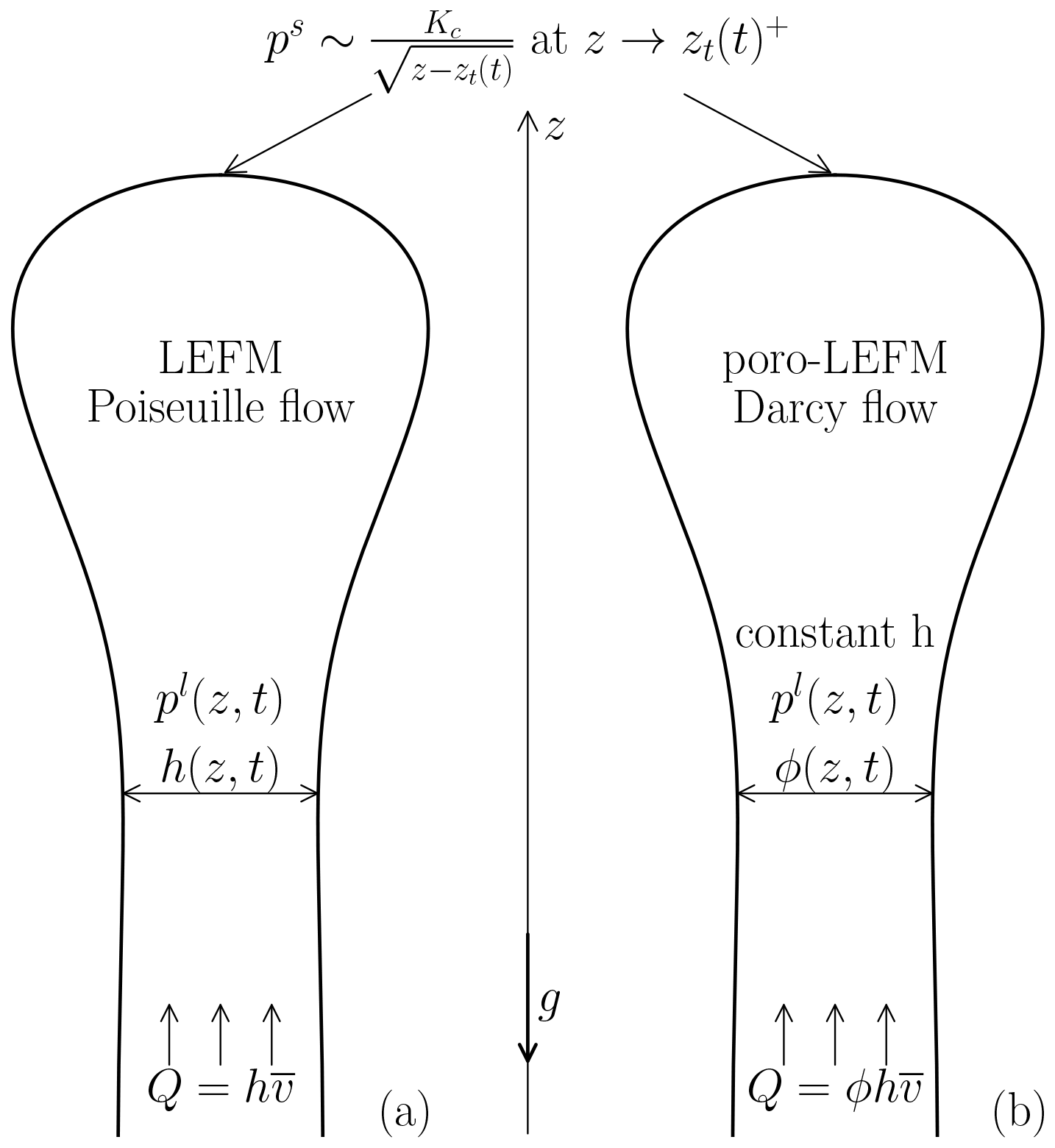
Figure 1 Sketch of the LEFM (e.g. Lister, 1990) and poro-LEFM models for a buoyancy-driven fracture. Here, Q denotes the volume flux through the fracture, and $\stackrel{\mathrm{‾}}{v}$ represents the cross-section average of vertical velocity component of the liquid. Both Q and $\stackrel{\mathrm{‾}}{v}$ are constants at $z\to -\mathrm{\infty }$. The far-field conditions and the definition of other notations are presented in Sect. 2.

LEFM models have explored the propagation rate and geometry of two-dimensional fractures with constant flux (Lister, 1990; Roper and Lister, 2007), as well as two- and three-dimensional fractures with constant volume (Spence and Turcotte, 1990; Davis et al., 2020, 2023). These magmatic fractures can be slowed or arrested due to loss of volatiles and heat and by solidification (Rubin, 1995; McLeod and Tait, 1999; Bolchover and Lister, 1999; Taisne et al., 2011; Rivalta et al., 2015; Abdullin et al., 2024). The direction of propagation has been investigated in relation to tectonic stress, topographic loading, and crustal heterogeneity (Maccaferri et al., 2014; Acocella et al., 2024). Despite the many successes of the LEFM approach, there are significant obstacles to consistently embedding it into models that account for the causes, dynamics, and consequences of dyking.

In the geodynamic context of the hot, ductile asthenosphere, magma transport has long been modelled using a poro-viscous Stokes–Darcy theory (e.g. McKenzie, 1984; Katz, 2022). This two-phase continuum formulation has been applied to geological settings including mid-ocean ridges (e.g. Sim et al., 2020; Pusok et al., 2022b), subduction zones (e.g. Rees Jones et al., 2018; Cerpa et al., 2018), and beneath continents (e.g. Schmeling et al., 2019). These studies were limited to hot asthenospheric regions by the use of a purely viscous rheological law.

In other work, the theory has been extended to accommodate elastic and brittle deformation at lower temperatures, where a solely viscous response to stress is inadequate to capture the mechanics (e.g. Connolly and Podladchikov, 1998; Bercovici et al., 2001; Kaus and Podladchikov, 2006; Burov, 2011; Cai and Bercovici, 2013; Keller et al., 2013; Kiss et al., 2023). This extension aimed to model melt transport upwards across the ductile–brittle transition. Notably, Keller et al. (2013) first incorporated plastic failure into a two-phase continuum model of magmatism. Li et al. (2023) improved the theoretical formulation by employing a poro-viscoelastic–viscoplastic (poro-VEVP) rheology after Duretz et al. (2021) and by proposing a new hyperbolic yield surface (e.g. Abbo and Sloan, 1995; Carol et al., 1997) to address physical, mathematical, and computational issues of Keller's model. The present study uses the same numerical framework detailed in Li et al. (2023), which showed how dyke-like features emerge from this formulation and bear a quantitative similarity with dykes described by LEFM theory. In particular, Li et al. (2023) observed that a poro-VEVP dyke can be narrow and fast relative to advection and (de)compaction in poro-viscous dynamics (Kelemen et al., 1997; Katz et al., 2022), and the stress distribution around its tip matches the LEFM model for some value of critical stress intensity.

However, two significant differences between the poro-VEVP and LEFM theories are readily noted: Darcian versus Poiseuille flow of the liquid phase and plastic yield versus brittle fracture of the solid phase. Therefore, further exploration and validation of the capabilities of the continuum representation of dykes are necessary. In the comparison with LEFM, two major issues require further investigation. The first is the slower propagation speed predicted by the poro-VEVP formulation (∼1 m yr⁻¹ versus ∼1 km d⁻¹; Davis et al., 2023). The second is the very high critical stress intensity needed in LEFM for consistency between the predictions (∼1.5 GPa m${}^{\mathrm{1}/\mathrm{2}}$). The previous benchmark in Li et al. (2023) is also incomplete in that the poro-VEVP dyke was driven by far-field tensile stresses, not buoyancy, and did not reproduce the classic LEFM cases of constant flux or constant volume for comparison.

To organise our investigation of these issues, we propose two hypotheses. We hypothesise that the slow speed of poro-VEVP dyke propagation is due to the greater viscous resistance to magma ascent in Darcian porous flow compared to Poiseuille flow. Furthermore, we hypothesise that the fracture toughness that provides an equivalent resistance to dyke propagation can be directly calculated from the rate of plastic energy dissipation in the poro-VEVP model. We verify these hypotheses by simulating a constant-flux, buoyancy-driven fracture in the poro-VEVP model and making quantitative comparison to a corresponding LEFM model.

To facilitate the comparison, we introduce a modified LEFM model in which the interior of the dyke is a porous medium. This assumes a dyke region with fixed width but variable porosity (Fig. 1b). In this poro-LEFM model, Darcy flow supplies buoyant fluid to a toughness-dominated tip embedded in an elastic medium. The poro-LEFM model converges to the classical LEFM model in the limit of the porosity going to unity. However, at smaller porosity, it facilitates a direct comparison with the poro-VEVP model in terms of stress distribution, porosity profile, and dyke propagation speed. We show that through the use of a poro-LEFM fracture toughness, calculated with a poro-VEVP energy analysis, there is a good match between the two models. This establishes a physics-based, quantitative relation between the poro-VEVP and LEFM models. Moreover, it advances our understanding of how distributed plastic failure affects dyke propagation.

As we detail below, this comparison also highlights a shortcoming of the poro-VEVP model. Isotropic permeability within the poro-VEVP dyke promotes widening by horizontal porous flow, a behaviour not associated with real (or LEFM) dykes. We resolve this discrepancy by introducing an anisotropic permeability tensor into the two-dimensional poro-VEVP model to limit leakage and enhance fracture propagation (e.g. Snow, 1969). Anisotropic permeability can arise from anisotropic stresses and aligned pores or fractures (e.g. Snow, 1969; Sibson, 1996; Daines and Kohlstedt, 1997; Li et al., 2009; Takei, 2010; Taylor-West and Katz, 2015; Lei et al., 2017; Lang et al., 2018; Seltzer et al., 2023; Medici et al., 2023; Bader et al., 2024).

This paper is organised as follows. The next section (Sect. 2) develops the poro-LEFM model, details the poro-VEVP model, and explains how energy dissipation is used to evaluate fracture toughness. The Results section (Sect. 3) illustrates the steadily propagating dykes produced by the poro-VEVP model. The Results section also verifies the estimated toughness by comparing poro-VEVP and poro-LEFM models in terms of their porosity and stress distributions. We discuss the results and their broader relevance in Sect. 4 and summarise in Sect. 5.

2 Models of a buoyancy-driven dyke

In this section, we develop two distinct models that are both aimed to describe buoyancy-driven dyke ascent. We first introduce the poro-LEFM model, which differs from the standard LEFM model in that it treats the dyke interior as a porous medium (Sect. 2.1). We then review the continuum mechanical, poro-VEVP model developed in Li et al. (2023), and we equip it with two key enhancements: a reformulated compaction pressure for improved numerical robustness and anisotropic permeability to impose a preferred dyke-parallel direction of Darcy flow (Sect. 2.2). Finally, we develop an analysis of mechanical energy dissipation in the poro-VEVP representation of a dyke (Sect. 2.3). This energy analysis provides a quantitative estimate of the effective fracture toughness for the poro-LEFM model and hence a basis for comparing the models.

2.1 The poro-LEFM formulation

The development of the poro-LEFM model follows Lister (1990), both conceptually and mathematically. This section gives an overview; full details are available in Appendix A.

Similar to the classic LEFM model in Fig. 1a, we consider a vertical two-dimensional channel as shown in Fig. 1b, extending from −∞ to a tip at position z=z_t. This channel represents an idealised dyke where buoyant fluid flows upward, deforms the elastic solid phase, and drives the fracture at the tip. Along the fracture walls, the elastic normal stress p^s is intensified by a critical factor K_c near the tip.

Unlike the LEFM model, which assumes Poiseuille flow in an open channel of variable width, the poro-LEFM model assumes porous flow in a permeable channel of uniform, fixed width h and variable porosity ϕ(z,t). The porous flow is modulated by a porosity-dependent mobility $M_{\mathit{\varphi }}=k_{\mathit{\varphi }}/\mathit{\mu }$, where k_ϕ is the permeability and μ is the liquid viscosity. We assume that this porous flow is driven purely by buoyancy, leading to a constant porosity ϕ₀ in the tail region, which we refer to as the far field.

The mathematical formulation includes Darcy's law for the liquid flux ϕv, an elastic-stress-balance equation, and boundary conditions at the tip and far field,

$$\begin{array}{}\text{(1)}& {\displaystyle }& {\displaystyle }\mathit{\varphi }v=M_{\mathit{\varphi }}\left(-{\displaystyle \frac{\partial p^{\mathrm{l}}}{\partial z}}+\mathrm{\Delta }\mathit{\rho }g\right),\text{(2)}& {\displaystyle }& {\displaystyle }{p}^{\mathrm{s}}(z,t)=-\left({\displaystyle \frac{G}{\mathrm{1}-\mathit{\nu }}}\right){\displaystyle \frac{\mathrm{1}}{\mathrm{2}\mathit{\pi }}}\underset{-\mathrm{\infty }}{\overset{\mathrm{\infty }}{\int }}{\displaystyle \frac{\partial h\mathit{\varphi }(\mathit{\xi },t)}{\partial \mathit{\xi }}}{\displaystyle \frac{\mathrm{d}\mathit{\xi }}{\mathit{\xi }-z}},\text{(3)}& {\displaystyle }& {\displaystyle }{p}^{\mathrm{s}}(z,t)\approx -{\displaystyle \frac{K_{\mathrm{c}}}{{\left[\mathrm{2}\left(z-z_{\mathrm{t}}\right)\right]}^{\mathrm{1}/\mathrm{2}}}},\mathrm{at}z\to z_{\mathrm{t}}^{+},\text{(4)}& {\displaystyle }& {\displaystyle }\mathit{\varphi }\approx {\mathit{\varphi }}_{\mathrm{0}},\mathrm{at}z\to -\mathrm{\infty }.\end{array}$$

Here v is the vertical component of liquid velocity, p^l is the dynamic liquid pressure (assumed equal to p^s inside the dyke), $\mathrm{\Delta }\mathit{\rho }={\mathit{\rho }}^{\mathrm{s}}-{\mathit{\rho }}^{\mathrm{l}}$ is the density difference between solid (s) and liquid (l), g is the gravitational force per unit mass, G and ν are the elastic shear modulus and Poisson's ratio of the solid, and K_c is the critical stress intensity. In this paper, we select $\mathit{\nu }=\mathrm{1}/\mathrm{2}$, which enforces that the solid phase is incompressible. Note that Eq. (2) adapts the standard LEFM elastic-stress formulation (e.g. Lister, 1990) to account for porosity effects on solid deformation.

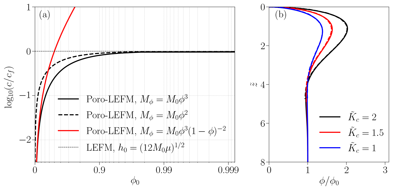
Figure 2 Comparison of LEFM and poro-LEFM models. (a) Tip propagation speed as a function of melt fraction. The horizontal axis is presented in a logarithmic scale. Three different permeability–porosity relationships are considered in the poro-LEFM model. The mobility prefactor M₀ is defined as $M_{\mathrm{0}}=h_{\mathrm{0}}^{\mathrm{2}}/\mathrm{12}\mathit{\mu }$, ensuring that c→c_f when ϕ₀→1. (b) Profiles of porosity at different values of ${\stackrel{\mathrm{̃}}{K}}_c$ in the poro-LEFM model (solid lines) compared with the profiles of scaled fracture width $h/h_{\mathrm{0}}$ in the LEFM model (dashed lines) (Lister, 1990, Fig. 3).Here, ${\stackrel{\mathrm{̃}}{K}}_c$ and $\stackrel{\mathrm{̃}}{z}$ denote scaled K_c and z, respectively.

For a purely buoyancy-driven flow, buoyancy is balanced by the Darcian drag force, and the propagation speed c becomes constant. This speed is obtained by solving Eq. (1) for v as $z\to -\mathrm{\infty }$, where there is no gradient of dynamic pressure,

$$\begin{array}{}\text{(5)}& c={\displaystyle \frac{M_{\mathit{\varphi }}\left({\mathit{\varphi }}_{\mathrm{0}}\right)}{{\mathit{\varphi }}_{\mathrm{0}}}}\mathrm{\Delta }\mathit{\rho }g.\end{array}$$

Here M_ϕ(ϕ₀) is the fluid mobility at ϕ=ϕ₀. This implies a constant volume flux from the far field: Q₀≡ϕ₀hc. We compare this result with a canonical LEFM, buoyancy-driven, open fracture having far-field width h₀ and hence tip speed $c_{\mathrm{f}}=h_{\mathrm{0}}^{\mathrm{2}}\mathrm{\Delta }\mathit{\rho }g/\mathrm{12}\mathit{\mu }$ (Lister, 1990).

Figure 2a shows how the poro-LEFM steady propagation speed c increases with the far-field porosity ϕ₀ for two choices of fluid mobility: a power-law relation M_ϕ=M₀ϕⁿ, where n=2 and 3, and the Kozeny–Carman relation $M_{\mathit{\varphi }}=M_{\mathrm{0}}{\mathit{\varphi }}^{\mathrm{3}}(\mathrm{1}-\mathit{\varphi }{)}^{-\mathrm{2}}$. We choose $M_{\mathrm{0}}=h_{\mathrm{0}}^{\mathrm{2}}/\mathrm{12}\mathit{\mu }$ to achieve a convergence between c and c_f. In particular, with our choice of M₀ in the power-law permeability relation, the speed c approaches c_f as ϕ₀→1. We adopt the cubic porosity dependence for the remainder of this paper to enforce a quantitative relationship between poro-LEFM and canonical LEFM theory.

We solve the system of equations and boundary conditions (Eqs. 1–4) after rescaling variables and transforming into a coordinate system that moves with the tip (see Appendix A for details). Solutions for ϕ(z) are obtained with the numerical procedure given by Roper and Lister (2007).

Figure 2b presents results for three choices of K_c. The porosity is non-dimensionalised by the far-field porosity ϕ₀. All porosity profiles show a bulging head approaching the tip at which ϕ=0 and a constant value in the tail where ϕ=ϕ₀. The head widens (again, in terms of the porosity) with increasing K_c, giving a larger solid deformation and therefore reflecting the increasing stress required to propagate the tip.

Figure 2 verifies the anticipated alignment between the poro-LEFM and LEFM models. Figure 2a displays the convergence of propagation speeds when M₀ is judiciously selected as noted above. It is important to recognise that for the far-field volume flux to converge as ϕ→1, the poro-LEFM width must equal the far-field width of the LEFM dyke, meaning h=h₀. Figure 2b shows the quantitative equivalence between the porosity distribution in a poro-LEFM dyke and the width variation in an LEFM dyke in dimensionless terms, corroborated by the numerical results from Lister (1990). This equivalence is also clear by comparing the dimensionless equations Eqs. (A10)–(A13) in Appendix A with Eqs. (2.8)–(2.10) of Lister (1990).

2.2 The poro-viscoelastic–viscoplastic (poro-VEVP) formulation

This section presents a two-dimensional (2D) Stokes–Darcy model for simulating a buoyancy-driven dyke with constant liquid influx from the boundary. This model shares Darcy's equation and mass continuity equation with the poro-LEFM model but in 2D form and taking into account the solid velocity. The stress-balance equation for the solid phase is more complex, balancing stresses of the two-phase medium in the context of a poro-viscoelastic–viscoplastic (poro-VEVP) rheological law. The solid phase deforms as a Maxwell material combining viscous, elastic, and viscoplastic elements, with a Kelvin viscosity for regularisation of plasticity. For more details on this poro-VEVP model, see Li et al. (2023). Here, we focus on improvements to the poro-VEVP model for simulating a constant-width, fluid-driven fracture in a porous medium and explain the computational model setup.

2.2.1 Stress-balance equation and a new compaction formulation

Stress balance of a two-phase medium satisfies

$$\begin{array}{}\text{(6)}& -\mathrm{\nabla }{p}^{\mathrm{l}}+\mathrm{\nabla }\cdot \left[(\mathrm{1}-\mathit{\varphi }){\mathit{\tau }}^{\mathrm{s}}\right]-\mathrm{\nabla }\left[(\mathrm{1}-\mathit{\varphi })\mathrm{\Delta }P\right]-\mathit{\varphi }\mathrm{\Delta }\mathit{\rho }\mathit{g}=\mathbf{0}.\end{array}$$

Here, (1−ϕ)τ^s and $-(\mathrm{1}-\mathit{\varphi })\mathrm{\Delta }P$ represent the effective shear and decompaction stresses, respectively. These are components of Terzaghi's effective stresses (Terzaghi, 1943). $\mathrm{\Delta }P=p^{\mathrm{s}}-p^{\mathrm{l}}$ is the pressure difference between phases (hereafter referred to as overpressure, following the convention in, for example, Keller et al., 2013, and Li et al., 2023). The shear and decompaction stresses must be expressed in terms of strain rates and must also be constrained by the plastic yield condition. This challenge was addressed by Li et al. (2023), and we follow their approach, with a small modification.

Previous studies employed an effective viscosity method for both shear and compaction (e.g. Moresi et al., 2003; Keller et al., 2013; Li et al., 2023). While this approach is appropriate for shear, it can lead to a divergence of the effective compaction viscosity during plastic failure, compromising computational robustness (Appendix B). We propose a new formulation of ΔP to resolve this, which compares with the old formulation as follows,

$$\begin{array}{}\text{(7)}& {\displaystyle }& {\displaystyle }\mathrm{Old}\mathrm{formulation}:(\mathrm{1}-\mathit{\varphi })\mathrm{\Delta }P=-{\mathit{\zeta }}_{\mathrm{eff}}{\mathcal{C}}^{\prime },\text{(8)}& {\displaystyle }& {\displaystyle }\mathrm{New}\mathrm{formulation}:(\mathrm{1}-\mathit{\varphi })\mathrm{\Delta }P=-{\mathit{\zeta }}^{\mathrm{ve}}{\mathcal{C}}^{\prime }+(\mathrm{1}-\mathit{\varphi })\mathrm{\Delta }{P}_{\mathrm{dl}},\end{array}$$

where

$$\begin{array}{}\text{(9)}& {\mathcal{C}}^{\prime }=\left[\mathcal{C}-{\displaystyle \frac{(\mathrm{1}-\mathit{\varphi })\mathrm{\Delta }{P}^{\mathrm{o}}}{Z_{\mathit{\varphi }}\mathrm{\Delta }t}}\right],{\mathit{\zeta }}^{\mathrm{ve}}={\left({\displaystyle \frac{\mathrm{1}}{{\mathit{\zeta }}_{\mathit{\varphi }}^{\mathrm{v}}}}+{\displaystyle \frac{\mathrm{1}}{Z_{\mathit{\varphi }}\mathrm{\Delta }t}}\right)}^{-\mathrm{1}}.\end{array}$$

Here, 𝒞 is the solid decompaction rate, ${\mathit{\zeta }}_{\mathit{\varphi }}^{\mathrm{v}}$ and Z_ϕ are the compaction viscosity and bulk modulus, Δt is the time step, and ΔP^o is the overpressure in the previous time step. Both the effective viscosity ζ_eff in the old formulation and the term we refer to as the dilatancy pressure, (1−ϕ)ΔP_dl, in the new formulation are parameters utilised to enforce the plastic yielding limit in the stress-balance equation. This is achieved using Picard iterations as an outer loop that wraps around the velocity–pressure solver to achieve global stress balance. This iterative scheme enforces the plastic yielding limit by updating the relevant parameter (ζ_eff or ΔP_dl) in each iteration. The details of this implementation can be found in Appendix D of Li et al. (2023).

When the plastic yield limit is not reached, ζ_eff=ζ^ve and ΔP_dl=0, making the two formulations equivalent. During plastic yield, ΔP is calculated from the plastic model, and either formulation can be rearranged to obtain the corresponding parameter while maintaining a fixed 𝒞^′. The old formulation calculates the effective compaction viscosity as ${\mathit{\zeta }}_{\mathrm{eff}}=(\mathrm{1}-\mathit{\varphi })\mathrm{\Delta }P/{\mathcal{C}}^{\prime }$, and feeds ζ_eff to the stress-balance equation as a constant, which becomes infinity when ${\mathcal{C}}^{\prime }=\mathrm{0}$. This infinite ζ_eff impacts the convergence of the solver for the velocity field from the stress-balance equation. The new formulation resolves this issue by calculating $(\mathrm{1}-\mathit{\varphi })\mathrm{\Delta }{P}_{\mathrm{dl}}=(\mathrm{1}-\mathit{\varphi })\mathrm{\Delta }P+{\mathit{\zeta }}^{\mathrm{ve}}{\mathcal{C}}^{\prime }$ instead, and feeding it to the stress-balance solver as a constant. The new constant always remains finite, improving the robustness of the computational codes.

2.2.2 Anisotropic permeability due to plastic failure

In the poro-VEVP model, a direct comparison with the essentially one-dimensional poro-LEFM model in Sect. 2.1 requires that the simulated dyke maintains a constant width. With an isotropic permeability, however, a vertical porous dyke would inevitably widen over time due to a Darcy flux in the horizontal direction. To prevent this methodologically undesirable leakage, we introduce an anisotropic permeability (Snow, 1969). It is critical to note that the purpose of this anisotropy is to confine the flow vertically for the benchmarking exercise, not to simulate the complex geological controls that guide dyke trajectories in nature. The formulation, detailed below, enhances permeability parallel to the direction of maximum tensile plastic strain, thereby keeping the dyke confined to a single column of cells.

Anisotropic permeability can be thought of as a macroscopic representation of melt-preferred orientation (MPO), which refers to the alignment of interconnected, melt-filled pores at the grain scale in partially molten rocks (e.g. Daines and Kohlstedt, 1997; Takei, 2010; Bader et al., 2024). Under the effect of differential stresses, these pores align and elongate perpendicular to the direction of maximum tension, causing differences in fluid transmissivity in different directions.

Mode-I fractures in a porous medium, from grain-scale microcrack damage to fractures that span large numbers of grains, have an effect on liquid permeability that is similar to MPO. They create anisotropic permeability that favours flow along the fracture. Indeed, macroscopic mode-I fractures have been conceptualised as the result of the propagation of microcracks under tension, with the propagation direction perpendicular to the direction of maximum tension (e.g. Griffith, 1921; Murrell, 1964). Aligned microcracks are closely analogous to aligned, elongated pores. We therefore assume that mode-I fractures also cause an anisotropic permeability.

To incorporate permeability anisotropy, we use a rank-2 tensor M_ϕ to express the liquid mobility, with a size matching the problem's dimensionality. Darcy's equation is then written as

$$\begin{array}{}\text{(10)}& \begin{array}{rl}\mathit{\varphi }\left({\mathit{v}}^{\mathrm{l}}-{\mathit{v}}^{\mathrm{s}}\right)=& -{\mathbf{M}}_{\mathit{\varphi }}\cdot \left(\mathrm{\nabla }{p}^{\mathrm{l}}+\mathrm{\Delta }\mathit{\rho }\mathit{g}\right),\\ & \mathrm{where}{\mathbf{M}}_{\mathit{\varphi }}=M_{\mathrm{0}}{\mathit{\varphi }}^n{\mathbf{M}}_{\mathrm{a}}.\end{array}\end{array}$$

Here, v^l and v^s represent liquid and solid velocity, respectively. M_a represents the anisotropic modification. When M_a is the identity tensor, the mobility is isotropic, and the equation above becomes the standard Darcy equation.

For vertically propagating dykes simulated in this paper, M_a is a diagonal matrix,

$$\begin{array}{}\text{(11)}& {\mathbf{M}}_{\mathrm{a}}=\left(\begin{array}{cc}{k}_{xx}& \mathrm{0}\\ \mathrm{0}& k_{zz}\end{array}\right),\mathrm{where}{k}_{xx},k_{zz}\in \left(\mathrm{0},k_{\mathrm{a}}\right).\end{array}$$

Here, k_a is a prescribed maximum permeability enhancement. We define k_xx and k_zz based on the plastic strain components, $e_{xx}^{\mathrm{K}}$ and $e_{zz}^{\mathrm{K}}$; for example,

$$\begin{array}{}\text{(12)}& k_{xx}={\displaystyle \frac{k_{\mathrm{a}}}{\mathrm{1}+\left(k_{\mathrm{a}}-\mathrm{1}\right)\exp (r_{xx}/\mathit{ϵ})}},\mathrm{with}{r}_{xx}={\displaystyle \frac{e_{xx}^{\mathrm{K}}}{e_{xx}^{\mathrm{K}}+e_{zz}^{\mathrm{K}}}}-{\displaystyle \frac{\mathrm{1}}{\mathrm{2}}}.\end{array}$$

Similarly, k_zz is defined in terms of r_zz, which is written by replacing $e_{xx}^{\mathrm{K}}$ with $e_{zz}^{\mathrm{K}}$ in the numerator of r_xx. In Eq. (12) and its variant for k_zz, the quantities r_xx and r_zz measure the anisotropy of accumulated plastic strain in the x and z directions, respectively. Both are equal to 0 when $e_{xx}^{\mathrm{K}}=e_{zz}^{\mathrm{K}}$, leading to $k_{xx}=k_{zz}=\mathrm{1}$, indicating isotropic mobility. The anisotropy of mobility is related to the anisotropy of plastic strain by ϵ∼5 %, a characteristic scale of strain anisotropy. As we model only small deformations in this paper, we neglect advection of plastic strains.

2.2.3 Rheological parameters

To facilitate comparison with the poro-LEFM model, we aim to align the rheology of the poro-VEVP model as closely as possible. Moreover, our focus here is on relating plastic deformation in a two-phase continuum to fluid-driven fracture. Therefore, we suppress viscous deformation by assigning effectively infinite values to both the shear and compaction viscosity. Furthermore, we assign a relative small, constant value to the Kelvin viscoplastic viscosity η^K. The impact of this viscosity is discussed in Sect. 2.3.

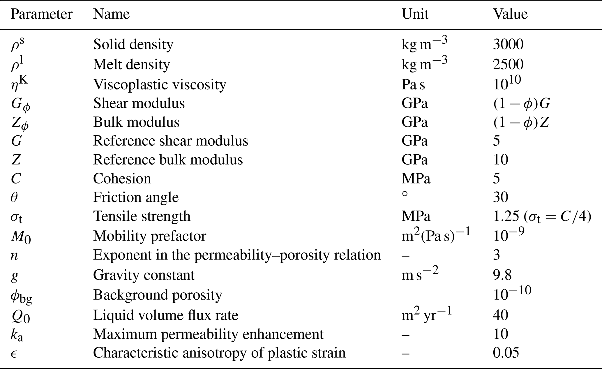
The elastic shear (G_ϕ) and bulk (Z_ϕ) moduli follow porosity-dependent relationships, as shown in Table 1. Note that this bulk modulus relates to the compaction of a solid–liquid aggregate, not to the compressibility of the solid phase. In fact, we assume that the solid phase is incompressible, which is enforced in the mass conservation equation.

Table 1 Dimensional parameters for computational modelling.

2.2.4 Computational model

The governing equations, detailed in Appendix C, are discretised on a staggered grid and solved using a finite-difference method. This numerical framework, including the implementation of the poro-VEVP rheology, closely follows the approach in Li et al. (2023). We solve the momentum and mass conservation equations using the FD-PDE framework (Pusok et al., 2022a), built on PETSc (Balay et al., 2022a). The model domain Ω is a tall rectangle, 2.44 km in width and 20 km in height. It is discretised using a 61×500 grid with a cell size of $\mathrm{\Delta }x=\mathrm{\Delta }z=\mathrm{40}$ m. We refer to the bottom boundary as B. A short time step of Δt=1 year is chosen to ensure solution accuracy. This time step is reduced further when the maximum permeability enhancement (k_a) increases. Details are discussed in Sect. 3.1.

The model is initiated with a prescribed porosity field designed to facilitate a direct comparison with the one-dimensional poro-LEFM model which is infinitely long in the z direction. The initial porosity field has a maximum value of 0.2 at the centre of B. The initial porosity decays laterally with a length scale of 10⁻⁴ km and vertically with scale 0.8 km according to a Gaussian function. This effectively prescribes an initial porous region having a width of one grid cell (40 m). Within this region, the porosity varies only vertically – not horizontally. This setup intentionally determines the location where the dyke will form, ensuring only one dyke is formed and that it propagates vertically through the middle of the domain. While this initial condition guides formation, the dynamics of the dyke's propagation – associated with localised plastic tensile failure – is not prescribed. It emerges from the solution of the governing equations when stresses exceed the plastic yield limit.

To exclude the effect of external forces on the solution within the domain, we prescribe zero shear and normal stresses on all boundaries except the bottom. Along B, we prescribe zero shear stress and zero normal velocity of the solid phase. Liquid flows across B at a constant volume rate Q₀ given by

$$\begin{array}{}\text{(13)}& Q_{\mathrm{0}}=\underset{B}{\int }{M}_{\mathrm{0}}{\mathit{\varphi }}^n{k}_{zz}\left(-{\displaystyle \frac{\partial p^{\mathrm{l}}}{\partial z}}+\mathrm{\Delta }\mathit{\rho }g\right)\mathrm{d}x.\end{array}$$

This is an integral of the vertical component of Eq. (10) over B. Assuming a constant pressure gradient ($\partial p^{\mathrm{l}}/\partial z$) in the region where ϕ>0 at the bottom boundary, we can rearrange Eq. (13) as a boundary condition for $\partial p^{\mathrm{l}}/\partial z$.

As we demonstrate below, this combination of domain, boundary, and initial conditions is an appropriate choice to simulate the poro-VEVP equivalent of dykes. We analyse their behaviour with reference to the poro-LEFM dyke model.

It should be noted that we do not prescribe the pressure gradient at the bottom boundary of the poro-VEVP model as $\partial p^{\mathrm{l}}/\partial z=\mathrm{0}$, which is the far-field condition of the poro-LEFM model. This is primarily due to the limitation inherent in the finite computational domain and further affected by the two-dimensionality in the poro-VEVP model. Firstly, a finite domain cannot simulate an infinitely long dyke; thus, the bottom boundary cannot be treated with a far-field condition. Secondly, unlike the poro-LEFM model which only considers horizontal displacement, the 2D continuum model allows for both vertical and horizontal deformation within the dyke due to solid phase (de)compaction. This results in a more complex solid stress tensor that must be balanced by the liquid pressure. These solid stresses remain significant even further away from the dyke tip, contrasting with the zero elastic solid pressure assumed in the poro-LEFM model (details in Appendix G). Given these restrictions, we define a constant liquid volume rate Q₀ instead. The propagation rate of the tip is a key point of comparison with the poro-LEFM model. To quantify it, we define a tip location z_t as the highest point along the vertical cross section at x=0 km where $\mathit{\varphi }\ge {\mathrm{10}}^{-\mathrm{3}}$. The tip speed is then diagnosed from the numerical results as $v_{\mathrm{t}}=\mathrm{d}{z}_{\mathrm{t}}/\mathrm{d}t$.

2.3 Energy analysis and the effective toughness

This section analyses the energy budget of the poro-VEVP model of a dyke. It estimates the effective fracture toughness in terms of the rate at which mechanical energy is dissipated by the propagation of the dyke tip.

In the poro-VEVP model, the total work rate $\dot{W}$ deforming the solid phase over a domain Ω is written as

$$\begin{array}{}\text{(14)}& \dot{W}=\underset{\mathrm{\Omega }}{\int }\dot{w}\mathrm{d}A,\mathrm{with}\dot{w}={\dot{w}}^{\mathrm{v}}+{\dot{w}}^{\mathrm{e}}+{\dot{w}}^{\mathrm{K}}.\end{array}$$

Here, $\dot{w}$ is the local work rate at a point, decomposed into viscous ${\dot{w}}^{\mathrm{v}}$, elastic ${\dot{w}}^{\mathrm{e}}$, and viscoplastic ${\dot{w}}^{\mathrm{K}}$ components for this Maxwell material. Appendix D provides details of the formulation for each local work rate. The total poro-VEVP work rate is similarly decomposed as

$$\begin{array}{}\text{(15)}& \dot{W}={\dot{W}}^{\mathrm{v}}+{\dot{W}}^{\mathrm{e}}+{\dot{W}}^{\mathrm{K}}.\end{array}$$

This can be compared with the (poro-)LEFM model, where the work rate includes elastic and fracture components,

$$\begin{array}{}\text{(16)}& {\dot{W}}_{\mathrm{LEFM}}={\dot{W}}_{\mathrm{LEFM}}^{\mathrm{e}}+{\dot{W}}_{\mathrm{LEFM}}^{\mathrm{f}},\end{array}$$

where the term with superscript “f” is the work rate to create new surface area of the fracture.

As a basis for comparison of a steadily propagating, constant flux, poro-VEVP dyke with a poro-LEFM dyke under the same conditions, we require that $\dot{W}={\dot{W}}_{\mathrm{LEFM}}$. Then, assuming that the elastic contributions to these work rates are approximately equal, we obtain a relationship between the dissipative parts,

$$\begin{array}{}\text{(17)}& {\dot{W}}^{\mathrm{v}}+{\dot{W}}^{\mathrm{K}}\approx {\dot{W}}_{\mathrm{LEFM}}^{\mathrm{f}}.\end{array}$$

We can use this result to diagnose a fracture toughness for the poro-VEVP model.

In LEFM theory, the energy expended to propagate the fracture a unit distance is commonly referred to as the strain energy release rate 𝒢. This variable is also interpreted as a measure of the material's fracture toughness in Anderson (2017), representing the resistance to fracture propagation. For simplicity, we refer to 𝒢 as the “fracture toughness” throughout this paper. We adopt the same definition of 𝒢 in the poro-LEFM model and assume a constant propagation speed c=v_t, i.e. an identical speed between the two formulations. Thus, the fracture energy rate is ${\dot{W}}_{\mathrm{LEFM}}^{\mathrm{f}}=\mathcal{G}{v}_{\mathrm{t}}$, which is the fracture energy budget per unit time. Combining this with Eq. (17), we calculate fracture toughness 𝒢 and critical stress intensity K_c from the dissipation rate of the poro-VEVP model as

$$\begin{array}{}\text{(18)}& \begin{array}{rl}\mathcal{G}& ={\displaystyle \frac{{\dot{W}}^{\mathrm{v}}+{\dot{W}}^{\mathrm{K}}}{v_{\mathrm{t}}}},\\ & K_{\mathrm{c}}={\left({\displaystyle \frac{\mathrm{2}G\mathcal{G}}{\mathrm{1}-\mathit{\nu }}}\right)}^{\mathrm{1}/\mathrm{2}}& ={\left[{\displaystyle \frac{\mathrm{2}G\left({\dot{W}}^{\mathrm{v}}+{\dot{W}}^{\mathrm{K}}\right)}{v_{\mathrm{t}}(\mathrm{1}-\mathit{\nu })}}\right]}^{\mathrm{1}/\mathrm{2}}.\end{array}\end{array}$$

The second equation is obtained from the LEFM relationship between the critical stress intensity factor and the fracture toughness for plane–strain deformation (Anderson, 2017), with substitution of the first equation for the fracture toughness in terms of the poro-VEVP dissipation rate.

As noted above, we suppress viscous deformation by prescribing a Maxwell viscosity that is effectively infinite (without changing the problem formulation). Because of this, we have ${\dot{W}}^{\mathrm{v}}\approx \mathrm{0}$; hence, the dissipation in the poro-VEVP model is entirely viscoplastic. Furthermore, we choose a small viscoplastic viscosity η^K to reduce the viscous dissipation in the Kelvin component. Appendix D2 discusses the effect of η^K on the rate of mechanical energy dissipation.

3 Results

The results are divided into two parts. First we document the output of the poro-VEVP model in terms of its dyke-like solutions. Second, we describe the comparison of those solutions to the poro-LEFM model.

3.1 Results of the poro-VEVP model

This section presents numerical solutions of the poro-VEVP model. We first analyse a reference case (parameters listed in Table 1) that demonstrates a steadily propagating dyke. We then investigate the effects of varying viscoplastic viscosity (η^K) and maximum permeability enhancement (k_a).

Figure 3a shows a snapshot of the porosity field from a representative numerical solution (see the video in the Supplement). The field includes a porous dyke with uniform width that rises up through the middle of the domain. A close-up investigation reveals that the central column of cells holds >90 % of the total volume of liquid in the domain. The porosity in laterally adjacent cells is at least 10 times smaller. This shows a negligible leakage through the wall and can confine the porous dyke to one cell in width. This width remains constant over time, enabling one-dimensional analysis along the central column of cells that represents the dyke. While advantageous in terms of comparison with a poro-LEFM model in which dykes are narrow relative to our grid spacing, this pattern raises questions about the grid-size dependence of the results. We address questions of grid-size dependence in Appendix E.

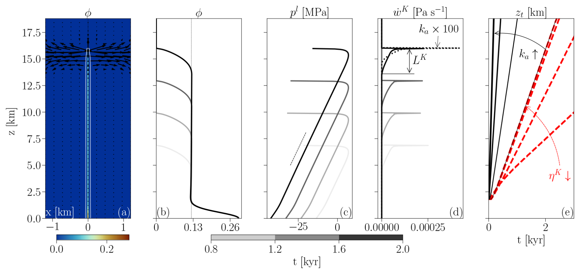
Figure 3 Results from a reference calculation of the poro-VEVP model. (a) Porosity and solid deformation field at t=2 kyr. The white curve represents the contour of $\mathit{\varphi }={\mathrm{10}}^{-\mathrm{3}}$. (b) Profiles of ϕ (solid lines) along a vertical cross section at x=0 for t=0.8, 1.2, 1.6, and 2.0 kyr. The dotted line represents ϕ=0.13. (c) Profiles of p^l along x=0 at the same time steps as (b). The slope in the tail region matches the poro-LEFM prediction with a prescribed flow rate and porosity (the dotted line). (d) The corresponding local plastic dissipation rate along x=0. Solid lines represent the reference case with k_a=10; the dotted line shows a case with k_a=10³ for comparison. The region below the tip with non-zero ${\dot{w}}^{\mathrm{K}}$ is referred to as the head region; its size is denoted L^K. (e) Tip propagation for different η^K (red) and k_a (black). Dashed red lines show propagation rate convergence for decreasing η^K (10¹⁸, 10¹⁷, 10¹⁶, and 10¹⁵ Pa s), as indicated by red arrows. The last one converges to the reference case, 10¹⁰ Pa s (thin solid line), with a speed of v_t=7.6 m yr⁻¹, matching the poro-LEFM prediction. The black lines show the variation of propagation speed for k_a=10 (reference case), 10², 10³, and 10⁴.

Figure 3b–d illustrates the steady advance of the dyke tip and the liquid phase. Figure 3b depicts porosity ϕ; Fig. 3c depicts liquid pressure p^l; Fig. 3d depicts local plastic dissipation rate ${\dot{w}}^{\mathrm{K}}$. Each panel shows four curves at different times (0.8, 1.2, 1.6, and 2.0 kyr), confirming that the tip advances approximately the same distance in each 0.4 kyr interval. This constant speed implies that a dynamic equilibrium has been achieved at the moving tip, which is consistent with the assumptions of the LEFM model. In Fig. 3b there is a region at z<2 km where the interior solution adjusts to match the boundary condition. Above this, for all four times, there is a region with uniform ϕ≈0.13. The height of this region grows linearly with time. Above this uniform region, each curve has a region where the porosity varies from ϕ≈0.13 to 0 at the dyke tip.

Figure 3d shows that beneath the tip is a region where plastic work is done. Indeed the position of the tip is characterised by the spike in ${\dot{w}}^{\mathrm{K}}$. We define the head of the poro-LEFM dyke as where ${\dot{w}}^{\mathrm{K}}$ is non-zero – that is, the entire region experiencing plastic tensile failure. In the reference case, this region is about 2.4 km high and confined to the column of grid cells that contain liquid. This height reduces to about 1.3 km when the permeability enhancement is 100 times larger (dotted line). The head region has a prominent solid displacement rate as shown in Fig. 3a. At the dyke tip, Fig. 3c shows that the pressure gradient is nearly singular; this is the location of tensile yielding, also corresponding with the spike in dissipation rate.

The mechanics of the head region represent a key difference between the poro-VEVP and poro-LEFM models. In the poro-VEVP model, buoyancy induces plastic tensile failure throughout the head region, whereas in the poro-LEFM model, fracture is localised exclusively to the tip. This difference is reflected in the pattern of energy dissipation of each model: distributed over a finite zone in poro-VEVP versus localised to a point in poro-LEFM. It is also important to note that our yield criterion combines both shear and tensile failure (Li et al., 2023), which means that unlike in a poro-LEFM model, we cannot isolate a purely mode-I (tensile) fracture process.

The tail region in Fig. 3c shows another distinction between the two models. The poro-VEVP model has a constant, non-zero pressure gradient $\partial p^{\mathrm{l}}/\partial z\approx \mathrm{3.2}$ MPa km⁻¹ in the tail, contrasting to the zero far-field pressure gradient in the poro-LEFM model. This distinction stems from the limitations of the finite domain and the significant solid stress gradient, which necessitates a balancing liquid pressure gradient. This prevents the use of a zero pressure gradient as a boundary condition on the bottom, as explained in Sect. 2.2.4 and further detailed in Appendix G.

Figure 3e shows tip propagation at various values of viscoplastic viscosity η^K and permeability anisotropic enhancement k_a. All curves become linear in time after a short transient, indicating constant propagation speed. Speed increases as η^K decreases from 10¹⁸ Pa s but converges to a constant value below 10¹⁵ Pa s. Increasing k_a further increases the tip speed.

Figure 4a confirms the effect of k_a on v_t in a log–log plot, indicating a power-law relationship arising from the mobility closure,

$$\begin{array}{}\text{(19)}& v_{\mathrm{t}}\propto k_{\mathrm{a}}^{\mathrm{1}/\mathrm{3}},\end{array}$$

at constant influx rate. This relationship informs the choice of time-step size to ensure the accuracy by maintaining a moderate Courant number.

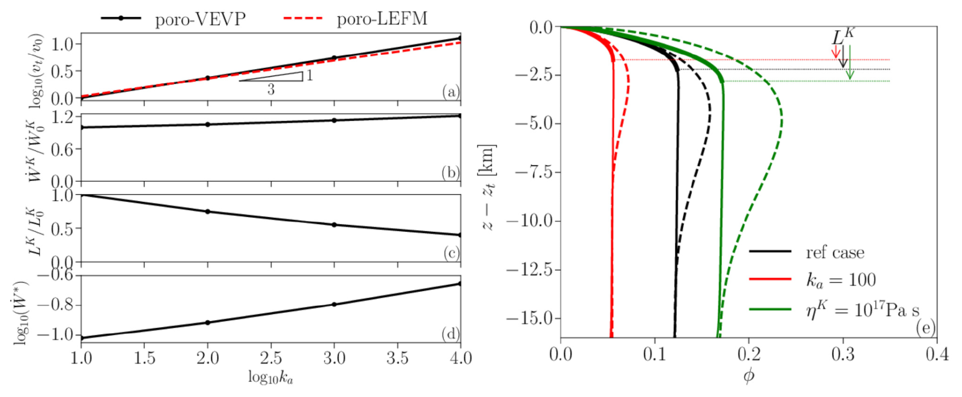
Figure 4 Key characteristics of simulated dykes as a function of the log of k_a. (a) The power-law relation between tip speed v_t and anisotropic permeability enhancement k_a. Here v_t is scaled by the speed in the reference case, v₀=7.6 m yr⁻¹. (b) The rate of plastic work ${\dot{W}}^{\mathrm{K}}$ increases with k_a but only by ∼7 % or less for each 10-fold increase of k_a. Here ${\dot{W}}^{\mathrm{K}}$ is scaled by the reference result ${\dot{W}}_{\mathrm{0}}^{\mathrm{K}}=\mathrm{3.1}$ Pa s⁻¹. (c) The size of plastic zone L^K decreases with k_a. The scaling factor is the reference result $L_{\mathrm{0}}^{\mathrm{K}}=\mathrm{2.4}$ km. (d) The dissipation intensity at the tip ${\dot{W}}^{*}$ increases with k_a. It measures the ratio of the dissipation rate in the tip cell to the overall rate. (e) Comparison of the porosity profiles of the poro-VEVP model (solid lines) with the poro-LEFM model (dashed lines). The critical stress intensities are K_c=0.51 (black), 0.34 (red), and 1.08 (green) GPa m${}^{\mathrm{1}/\mathrm{2}}$, calculated using the energy analysis of the poro-VEVP model (Eq. 18). Thicker solid lines indicate plastic zones in each case.

Figure 4a also demonstrates the agreement between the power-law relationship measured in poro-VEVP numerical solutions and the analytical prediction of the poro-LEFM model. Use of Darcy's law in the poro-LEFM model requires that Q₀∝M_ϕ for constant width, which translates to $Q_{\mathrm{0}}\propto k_{\mathrm{a}}{\mathit{\varphi }}_{\mathrm{0}}^n$ when fluid mobility is matched to the poro-VEVP model. This relationship indicates that, for a fixed Q₀, varying the permeability enhancement adjusts the far-field porosity according to ${\mathit{\varphi }}_{\mathrm{0}}\propto k_{\mathrm{a}}^{-\mathrm{1}/n}$. Given that Q₀=ϕ₀hc in the far field, the propagation speed must therefore scale as $c\propto k_{\mathrm{a}}^{\mathrm{1}/n}$. Recalling that we choose n=3, this scaling governs propagation speed in both models, despite their different values resulting from distinct pressure gradients in the tail region.

Figure 4b shows that the overall plastic dissipation rate increases with permeability enhancement but only by 20 % over a factor of 10³ change in k_a. This change is negligible compared to the 10-fold increase in propagation speed shown in Fig. 4a. Therefore, we can consider the total dissipation rate to be essentially independent of k_a. Recalling the calculation for fracture toughness and critical stress intensity in Eq. (18), we obtain the following power-law relationship for 𝒢 and K_c in terms of k_a,

$$\begin{array}{}\text{(20)}& \mathcal{G}\propto k_{\mathrm{a}}^{-\mathrm{1}/\mathrm{3}},K_{\mathrm{c}}\propto k_{\mathrm{a}}^{-\mathrm{1}/\mathrm{6}}.\end{array}$$

This contrasts with (poro-)LEFM models, where fracture toughness is independent of permeability, while the fracture energy rate changes in proportion to propagation speed.

Figure 4c and d show that larger permeability enhancement leads to a shorter plastic zone L^K, meaning a smaller head region and more intense plastic dissipation at the tip. This intensity is measured by the ratio of dissipation rate in the tip cell to the overall dissipation rate, ${\dot{W}}^{*}\equiv {\dot{w}}_{\mathrm{m}}^{\mathrm{K}}\mathrm{\Delta }x\mathrm{\Delta }z/{\dot{W}}^{\mathrm{K}}$. Here ${\dot{w}}_{\mathrm{m}}^{\mathrm{K}}$ denotes the work rate at the tip, which corresponds to the maximum value of curves in Fig. 3d. Given that ${\dot{W}}^{\mathrm{K}}$ is constant when fixing Q₀ and varying k_a, Fig. 4d also represents the variation of the peak dissipation rate ${\dot{w}}_{\mathrm{m}}^{\mathrm{K}}$ as a function of the permeability enhancement. Together, Fig. 4c and d indicate that increasing k_a reduces head height L^K and focuses plastic failure onto the tip. This trend provides an explanation for the reduction of fracture toughness associated with increasing k_a.

3.2 Comparison between the poro-VEVP and poro-LEFM models

This section compares the poro-VEVP and poro-LEFM dykes in terms of porosity profiles and stress distribution. We impose that the poro-LEFM dyke has the same width as the poro-VEVP dyke and has a far-field porosity equal to the tail-region porosity. Based on the energy analysis of the poro-VEVP results, we estimate an effective fracture toughness 𝒢 and thus a critical stress intensity factor K_c, which we then apply to the poro-LEFM model. In the comparison below, we evaluate whether this estimated K_c is an appropriate value to link these two models.

On the basis of this estimated K_c, Fig. 4e compares porosity profiles between the poro-VEVP (solid lines) and poro-LEFM (dashed lines) models. The panel shows three cases: the reference case (black), a case with increased viscoplastic viscosity η^K (green), and a case with increased maximum permeability enhancement k_a (red). When η^K is relatively small (black and red lines), the continuum and fracture models match well near the tip, suggesting that the plasticity-based K_c (and thus 𝒢) can quantitatively relate these two models. However, when η^K is relatively large (green), the two models are not closely aligned, even near the tip. Considering all three cases, we notice that the poro-VEVP dykes do not have the bulbous head which appears in the poro-LEFM dykes. What we have defined as the head in the poro-VEVP model (L^K), where plastic failure takes place, is much shorter than the head height in the poro-LEFM model.

Figure 5 compares components of the stress tensor between the two models in the zero-porosity region. The tensor is evaluated at points (blue dots in Fig. 5a) around a circle centred at the dyke tip and along a vertical line upwards from the tip (yellow dots in Fig. 5a). The stress calculation for the poro-LEFM is presented in Appendix F, which is identical to the LEFM model in the zero-porosity region. Figure 5b shows agreement of stress components between poro-VEVP and (poro-)LEFM along the azimuthal coordinate ϑ along a circle of radius r=160 m (=4Δx) in the region $\mathit{\vartheta }\in [-\mathrm{7}\mathit{\pi }/\mathrm{8},\mathrm{7}\mathit{\pi }/\mathrm{8}]$. Regarding the stress distribution along the radial direction, the (poro-)LEFM model predicts that σ_xx and σ_zz are both proportional to $\mathrm{1}/\sqrt{r}$, where r is distance from the tip. Figure 5c shows that the poro-VEVP results is somewhat but not entirely consistent with this prediction; ${\mathit{\sigma }}_{xx}\sim r^{-\mathrm{1}/\mathrm{2}}$ when r<5Δx, and ${\mathit{\sigma }}_{zz}\sim r^{-\mathrm{1}/\mathrm{2}}$ when $r\in [\mathrm{4},\mathrm{16}]\mathrm{\Delta }x$.

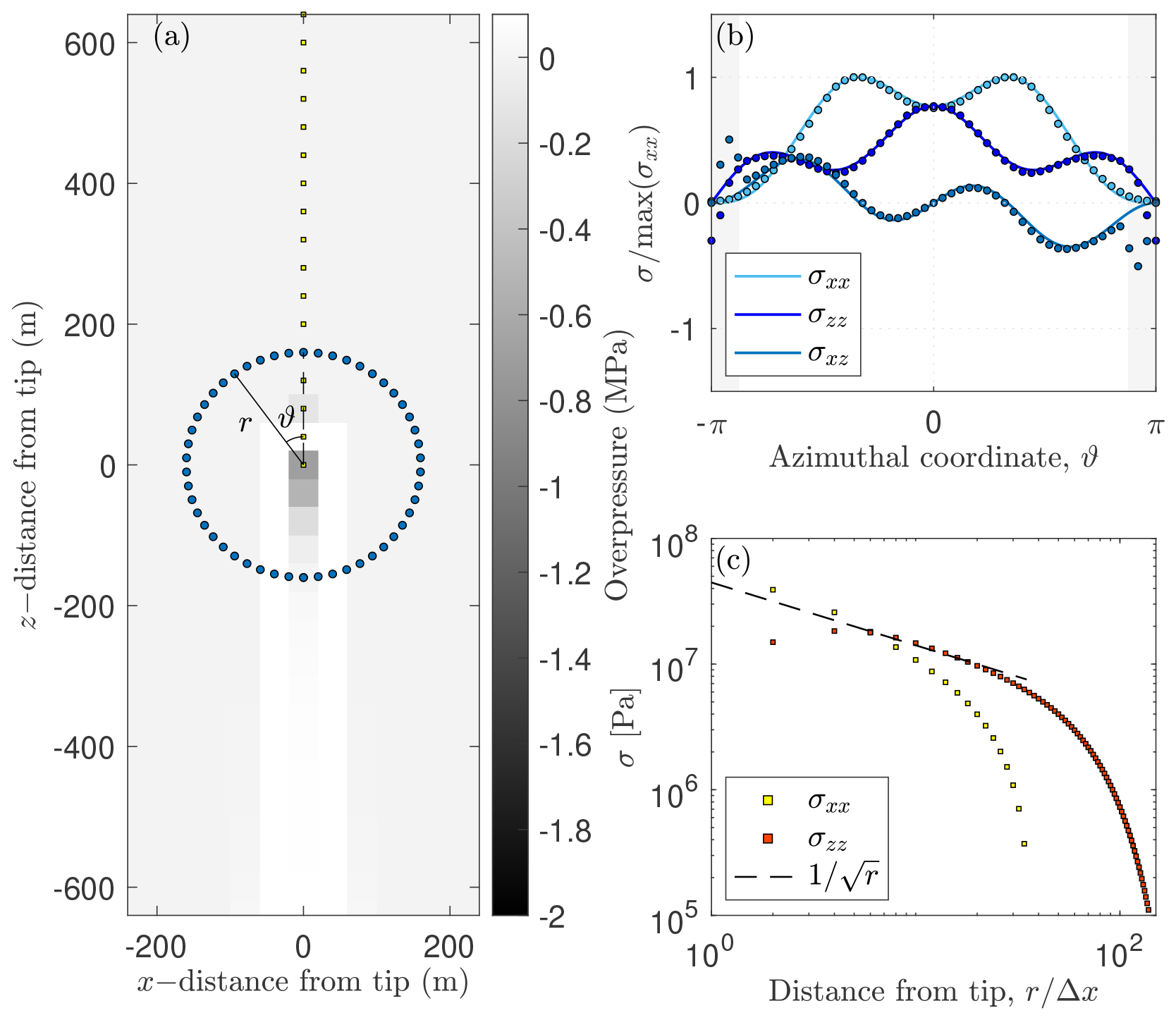
Figure 5 Comparison of stress components between the poro-VEVP model and the (poro-)LEFM model with K_c=510 MPa m${}^{\mathrm{1}/\mathrm{2}}$. (a) Fracture-tip coordinate system, where angle ϑ is measured counter-clockwise from the vertical axis and where radial distance r is measured from the origin. The background grey scale represents the liquid overpressure ΔP. (b) Fracture-tip stress distribution. LEFM solutions are depicted as solid lines, while poro-VEVP stress components as points evenly spaced in ϑ around the fracture at r=160 m (indicated by blue dots in panel a). Regions where $\left|\mathit{\vartheta }\right|>\mathrm{7}\mathit{\pi }/\mathrm{8}$ are shaded grey. (c) Fracture-tip stress asymptote. Squares represent poro-VEVP results directly ahead of the fracture tip (along ϑ=0; yellow points in panel a). The dashed line represents the LEFM $\mathrm{1}/\sqrt{r}$ singularity.

Li et al. (2023) made a similar comparison of the stress distribution between models but for the case of a dyke driven by uniform horizontal tension, imposed in the far field. The present paper enhances the credibility of such a comparison in two key ways: first, the poro-VEVP dyke is driven purely by buoyancy, consistent with the (poro-)LEFM dyke; second, the stress intensity factor is derived from the plastic dissipation rate of the poro-VEVP model, rather than using a fitted value.

4 Discussion

In the preceding sections, we compared poro-VEVP and LEFM models for simulating buoyancy-driven dykes. The comparison was facilitated by the introduction of an intermediary poro-LEFM model. This section discusses the results and addresses the slow propagation and high toughness of poro-VEVP dyking.

This study demonstrates that the poro-VEVP model can represent dykes with plastic tensile failure. Specifically, by incorporating anisotropic permeability, this model can simulate a long, thin dyke-like melt conduit with minimal liquid leakage through the walls, such that it is generally consistent with an LEFM model. The dyke width is determined by the grid size, which is a limitation of the present discretised solutions of the continuum models (see Appendix E for details). Despite this limitation, we can validate the poro-VEVP model against a poro-LEFM model, comparing the porosity and stress distributions of dykes with the same width.

The slow propagation speed of poro-VEVP dykes arises from the large drag on fluid motion under Darcy flow compared to Poiseuille flow in the LEFM model. This is quantified by the mobility M_ϕ, the ratio of permeability to liquid viscosity. Mobility is parameterised in terms of the product of a prefactor M₀ and a power of the porosity ϕ. While ϕ is part of the solution and cannot be directly manipulated to control the speed, M₀ can be increased within a dyke by prescribing a permeability enhancement k_a. Above we showed that the speed increases with k_a following the power law, $\propto k_{\mathrm{a}}^{\mathrm{1}/n}$, when the liquid volume influx is fixed. However, a faster dyke requires a smaller time step for accuracy, thereby increasing the computational cost. Therefore, when using the poro-VEVP model, consideration must be given to balancing the desire for more accurately representing rapid dyke propagation with the computational cost this incurs.

The fracture toughness of poro-VEVP dykes can be calculated from the plastic dissipation energy of the continuum model by assuming its equivalence to the fracture energy in the poro-LEFM model. In this way, we relate the toughness value to the speed of tip propagation and the size and intensity of the distributed plastic failure over a head region close to the dyke tip. This region is much shorter than the bulbous head in the poro-LEFM model, defined by where the porosity is distinct from the far-field porosity (2.4 km versus 12 km for the reference case). The finite-size failure region represents another difference to the poro-LEFM model, in which fracture occurs at the tip only. Despite this, by using the estimated toughness in the poro-LEFM model, we achieve reasonable agreement in the porosity profiles and stress distribution between the two models.

This toughness value is influenced by various physical parameters that alter the dynamics in the head region, including permeability enhancement (k_a), shear (G) and bulk (Z) moduli, cohesion (C), tensile strength (σ_t), and volume flux rate (Q₀). Figure 4 shows that increasing k_a leads to a decrease in 𝒢, while Fig. 6 demonstrates a positive correlation between 𝒢 and increasing values of G, C, σ_t, and Q₀. The elastic bulk modulus Z does not have a significant effect on 𝒢.

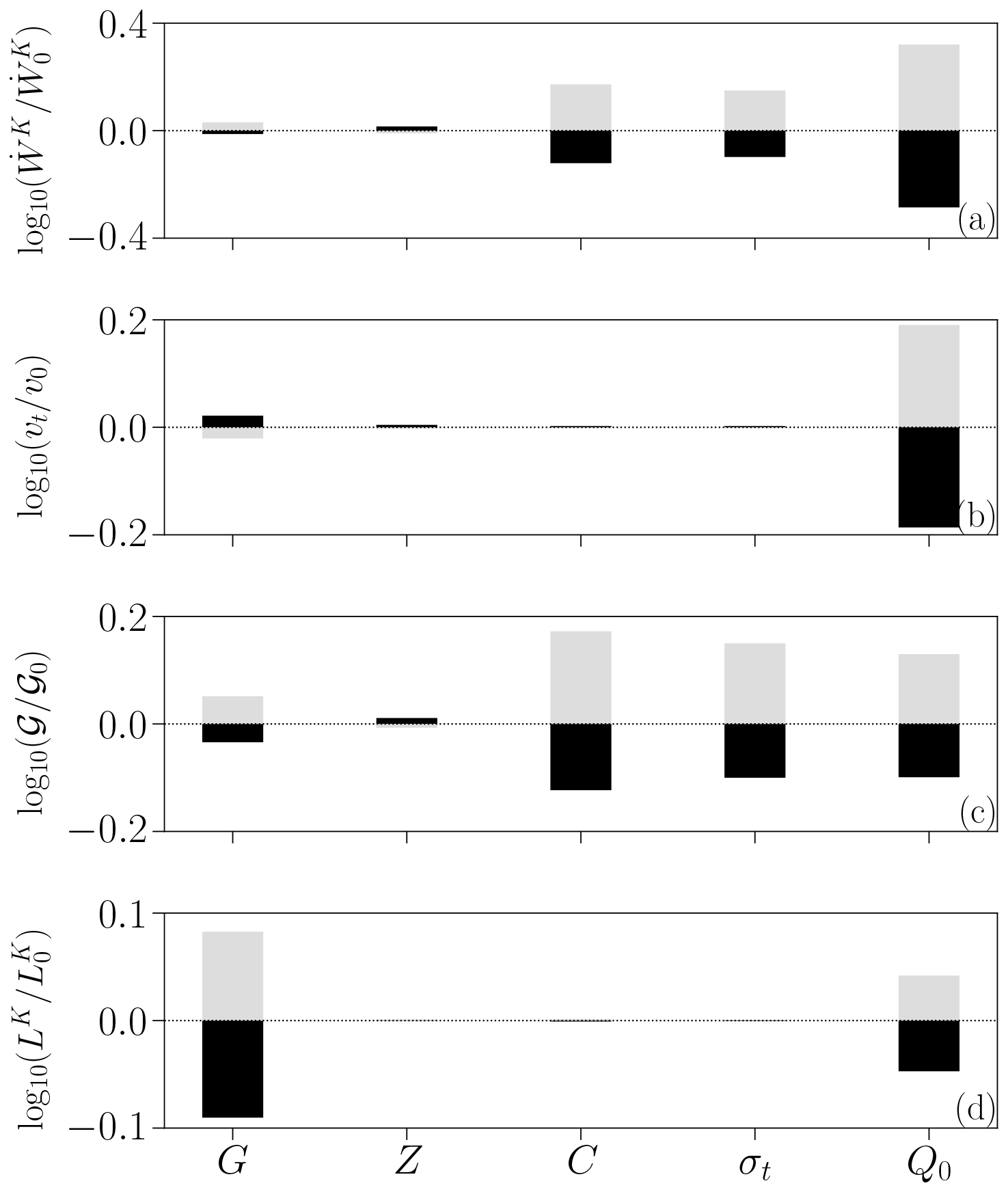
Figure 6 Dependence of the overall dissipation rate ${\dot{W}}^{\mathrm{K}}$, propagation speed v_t, fracture toughness 𝒢, and the head height L^K on the physical parameters: the shear modulus G, the bulk modulus Z, the cohesion C, the tensile strength σ_t, and the volume influx rate Q₀. Grey and black bars in each panel represent the variation of each variable by changing ×2 and $\times \mathrm{1}/\mathrm{2}$, respectively, on the reference value of each parameter. The variation is shown as the change relative to the corresponding result in the reference case.

These parameters affect fracture toughness in different ways. Increasing k_a reduces the head height (Fig. 4c) and localises dissipation to the tip (Fig. 4d), resulting in a reduced toughness. A similar relationship between the localisation of plastic dissipation and toughness is obtained by varying the elastic shear modulus (Fig. 6, first column). Increasing  G leads to increased toughness, accompanied by a longer plastic zone with a similar total dissipation rate, meaning a more distributed failure and taller head. Increasing cohesion and tensile strength also increases toughness, but it does so by increasing the overall dissipation rate without affecting the size of the plastic zone (Fig. 6, third and fourth columns). In these cases, the strength of plastic failure, rather than its distribution, is the primary factor associated with the variation of toughness. Furthermore, while a higher liquid volume flux increases the overall dissipation rate more than cohesion or tensile strength, it has a lesser effect on fracture toughness (Fig. 6, fifth column). This can be attributed to the increased propagation speed, which lowers the dissipation work per unit length of fracture growth.

The dependence of toughness on liquid volume flux is intriguing because, in the poro-LEFM model, liquid-phase dynamics do not affect solid properties. This may be explained in terms of two related ideas. First, the toughness as evaluated in poro-VEVP is associated with the energetics of the head region. This region has non-zero porosity, making the dissipation a property of the two-phase medium, i.e. something affected by the liquid phase. In contrast, the non-zero porosity in the poro-LEFM dyke does not affect the fracture energy because the fracture occurs precisely at the tip, where the porosity is zero.

Second, this sensitivity of toughness to liquid flux resembles that of more complex fracture mechanics theories like elastic plastic fracture mechanics (EPFM) (Anderson, 2017). EPFM applies a plastic yield limit to an elastic fracture-mechanics model. On this basis, it predicts a plastic zone around the fracture tip, where the intensified elastic stress reaches the yield limit. Papanastasiou (1999) uses EPFM to model a constant-flux, fluid-driven fracture, showing that a higher liquid flux leads to a larger plastic zone and, consequently, higher effective toughness and stress intensity. A large toughness and stress intensity in the poro-VEVP model can therefore be broadly related to plastic dissipation in the EPFM model. In fact, observations suggest that a large toughness might be possible in the field: Gudmundsson (2009) suggests a toughness value in volcanic edifices 2 orders of magnitude larger than that reported by laboratory experiments. Quantitatively aligning the poro-VEVP model with both EPFM model and field observations is beyond the present scope.

One limitation of the present research arises from the simplified form of anisotropic permeability that we impose. In particular, our formulation modifies only the horizontal or vertical permeability. This is appropriate if the dyke (or sill) aligns with one of these two directions, but it is unsuitable for modelling curved dyke trajectories, such as those influenced by ambient stresses (Maccaferri et al., 2014). Thus, the formulation of anisotropic permeability needs to be generalised to enable dyke propagation in an arbitrary direction. We will address this in future work.

Another limitation of this work is the difference in boundary conditions between poro-VEVP (constant volume flux, leading to a non-zero pressure gradient) and poro-LEFM (zero pressure gradient at the far-field). This is, however, unavoidable because of the limitations of the finite domain and also the two-dimensionality of the continuum model. As a result, the stresses between the solid and liquid balance differently inside of the dyke (see Appendix G for details). Nonetheless, we achieve a reasonable agreement between the two models near the tip by assuming the equivalence between plastic dissipation and fracture energy.

The plasticity model itself has limitations, some of which were discussed in Li et al. (2023). For instance, the model cannot distinguish between failure modes, and the dyke width is dependent on the grid resolution. Moreover, methods for plastic regularisation are an active area of research; for example, Duretz et al. (2023) make a comparison of three regularisation methods in the context of simulating shear failure (Duretz et al., 2023). A broader exploration of plasticity theory is, however, beyond the scope of this benchmarking study.

In conclusion, with some caveats, the representation of a dyke in the continuum, poro-VEVP formulation is consistent with linear elastic fracture mechanics. This consistency supports the validity of our approach for geodynamic applications. Moreover, it gives us confidence in incorporating poro-VEVP into large-scale rifting models requiring consistent magma transport in both ductile and brittle regions of the lithosphere (e.g. Pusok et al., 2025).

5 Summary

This study compares dyke propagation in a poro-viscoelastic–viscoplastic model with that in a canonical linear elastic fracture mechanics model. The comparison is enabled by interposing a novel poro-LEFM model. It highlights two key discrepancies: slow propagation speed of the poro-VEVP dyke and the requirement for large fracture toughness in the LEFM model to match the poro-VEVP results. We have reported on our progress in addressing these discrepancies.

Slow propagation speed in the poro-VEVP model is primarily attributed to low permeability relative to an open fracture. This limitation can be mitigated by introducing an anisotropic permeability enhancement. The large equivalent toughness value inferred for the poro-VEVP model can be explained in terms of plastic dissipation of mechanical energy. This effective fracture toughness depends on various physical parameters that affect the plastic dissipation rate in the solid–liquid aggregate. The poro-VEVP models now incorporates a new formulation for the constitutive relation between compaction stress and strain rates, which improves solver reliability over that used by (Li et al., 2023). Future development will focus on implementing the full anisotropic permeability tensor to investigate how the ambient stress field influences dyke (or sill) emplacement.

Appendix A: Mathematical formulation of the poro-LEFM model

This section provides details of the mathematical formulation of the poro-LEFM model that was introduced in Sect. 2.1. It explains how the governing equations of the liquid and solid phases are obtained and how they are non-dimensionalised.

A1 The liquid phase

We derive a mass continuity equation for the poro-LEFM model from Darcy's law and the mass conservation equation of a two-phase continuum model,

$$\begin{array}{}\text{(A1)}& {\displaystyle }& {\displaystyle }\mathit{\varphi }\left({\mathit{v}}^{\mathrm{l}}-{\mathit{v}}^{\mathrm{s}}\right)=-M_{\mathit{\varphi }}\left(\mathrm{\nabla }{P}^{\mathrm{l}}-{\mathit{\rho }}^{\mathrm{l}}\mathit{g}\right),\text{(A2)}& {\displaystyle }& {\displaystyle \frac{\partial \mathit{\varphi }}{\partial t}}+\mathrm{\nabla }\cdot \left(\mathit{\varphi }{\mathit{v}}^{\mathrm{l}}\right)=\mathrm{0}.\end{array}$$

We decompose the full liquid pressure gradient, ∇P^l, into static and dynamic components as

$$\begin{array}{}\text{(A3)}& \mathrm{\nabla }{P}^{\mathrm{l}}={\mathit{\rho }}^{\mathrm{s}}\mathit{g}+\mathrm{\nabla }{p}^{\mathrm{l}}.\end{array}$$

We denote the vertical component of liquid and solid velocity by v^l and v^s. Taking the vertical component of Eq. (A1) and assuming zero vertical solid velocity (v^s=0), we obtain the liquid flux rate as

$$\begin{array}{}\text{(A4)}& \mathit{\varphi }{v}^{\mathrm{l}}=M_{\mathit{\varphi }}\left(-{\displaystyle \frac{\partial p^{\mathrm{l}}}{\partial z}}+\mathrm{\Delta }\mathit{\rho }g\right).\end{array}$$

We assume zero horizontal component of liquid velocity, which implies no leakage through the fracture wall. Then Eq. (A2) reduces to

$$\begin{array}{}\text{(A5)}& {\displaystyle \frac{\partial \mathit{\varphi }}{\partial t}}+{\displaystyle \frac{\partial \mathit{\varphi }{v}^{\mathrm{l}}}{\partial z}}=\mathrm{0}.\end{array}$$

For an infinitely long buoyancy-driven dyke, we expect uniform propagation at a fixed speed with constant far-field porosity.

Assuming pure buoyancy drive (i.e. $\partial p^{\mathrm{l}}/\partial z=\mathrm{0}$ at the far field), Eq. (A4) yields the constant propagation speed,

$$\begin{array}{}\text{(A6)}& c={\displaystyle \frac{M_{\mathit{\varphi }}\left({\mathit{\varphi }}_{\mathrm{0}}\right)}{{\mathit{\varphi }}_{\mathrm{0}}}}\mathrm{\Delta }\mathit{\rho }g,\end{array}$$

where ϕ₀ is the far-field porosity. In this case, the far-field liquid volume rate is Q₀=ϕ₀hc.

A2 Solid and liquid stresses

We formulate the elastic solid stress distribution p^s(z,t) of the poro-LEFM model following the LEFM model (e.g. Weertman, 1971; Lister, 1990; Roper and Lister, 2007). This elastic stress, associated with dyke opening in the x direction, intensifies towards infinity at the tip, characterised by a critical stress intensity K_c.

The mathematical formulations are

$$\begin{array}{}\text{(A7)}& {\displaystyle }& {\displaystyle }{p}^{\mathrm{s}}(z,t)=-\left({\displaystyle \frac{G}{\mathrm{1}-\mathit{\nu }}}\right){\displaystyle \frac{\mathrm{1}}{\mathrm{2}\mathit{\pi }}}\underset{-\mathrm{\infty }}{\overset{\mathrm{\infty }}{\int }}{\displaystyle \frac{\partial h\mathit{\varphi }(\mathit{\xi },t)}{\partial \mathit{\xi }}}{\displaystyle \frac{\mathrm{d}\mathit{\xi }}{\mathit{\xi }-z}},\text{(A8)}& {\displaystyle }& {\displaystyle }{p}^{\mathrm{s}}(z,t)=-{\displaystyle \frac{K_{\mathrm{c}}}{{\left[\mathrm{2}\left(z-z_{\mathrm{t}}\right)\right]}^{\mathrm{1}/\mathrm{2}}}},\mathrm{at}z\to z_t^{+}.\end{array}$$

Here, hϕ represents the horizontal deformation required to open a porous dyke of width h with porosity ϕ, and z_t is the tip location.

We assume a force balance between the solid and liquid phases in the non-zero porosity region, so p^l=p^s across the dyke in the poro-LEFM model.

A3 Non-dimensionalisation

We transform the coordinate system to be fixed with respect to the fracture tip, changing (z,t) to $z^{\prime }\left(t\right)=(z_{\mathrm{t}}^{\mathrm{o}}+ct)-z$, where $z_{\mathrm{t}}^{\mathrm{o}}$ is the initial tip location.

We take the following non-dimensionalisation,

$$\begin{array}{}\text{(A9)}& \begin{array}{rl}& \stackrel{\mathrm{̃}}{\mathit{\varphi }}={\displaystyle \frac{\mathit{\varphi }}{{\mathit{\varphi }}_{\mathrm{0}}}},\stackrel{\mathrm{̃}}{z}=z^{\prime }{\left({\displaystyle \frac{Gh{\mathit{\varphi }}_{\mathrm{0}}}{(\mathrm{1}-\mathit{\nu })\mathrm{\Delta }\mathit{\rho }g}}\right)}^{-\mathrm{1}/\mathrm{2}},\\ & {\stackrel{\mathrm{̃}}{p}}^{\mathrm{s}}=p^{\mathrm{s}}{\left({\displaystyle \frac{Gh{\mathit{\varphi }}_{\mathrm{0}}}{(\mathrm{1}-\mathit{\nu })}}\mathrm{\Delta }\mathit{\rho }g\right)}^{-\mathrm{1}/\mathrm{2}},\\ & \stackrel{\mathrm{̃}}{K_{\mathrm{c}}}=K_{\mathrm{c}}{\left({\displaystyle \frac{Gh{\mathit{\varphi }}_{\mathrm{0}}}{\mathrm{1}-\mathit{\nu }}}\right)}^{-\mathrm{3}/\mathrm{4}}(\mathrm{\Delta }\mathit{\rho }g{)}^{-\mathrm{1}/\mathrm{4}}.\end{array}\end{array}$$

The system of governing equations (Eqs. 1–4) then leads to the following non-dimensionalised system,

$$\begin{array}{}\text{(A10)}& {\displaystyle }& {\displaystyle \frac{\mathrm{d}{\stackrel{\mathrm{̃}}{p}}^{\mathrm{s}}}{\mathrm{d}\stackrel{\mathrm{̃}}{z}}}={\left({\displaystyle \frac{\mathrm{1}}{\stackrel{\mathrm{̃}}{\mathit{\varphi }}}}\right)}^{\mathrm{2}}-\mathrm{1},\text{(A11)}& {\displaystyle }& {\displaystyle }{\stackrel{\mathrm{̃}}{p}}^{\mathrm{s}}\left(\stackrel{\mathrm{̃}}{z}\right)=-{\displaystyle \frac{\mathrm{1}}{\mathit{\pi }}}\underset{\mathrm{0}}{\overset{\mathrm{\infty }}{\int }}{\displaystyle \frac{\mathrm{d}\stackrel{\mathrm{̃}}{\mathit{\varphi }}\left(\mathit{\xi }\right)}{\mathrm{d}\mathit{\xi }}}{\displaystyle \frac{\mathrm{d}\mathit{\xi }}{\mathit{\xi }-\stackrel{\mathrm{̃}}{z}}},\text{(A12)}& {\displaystyle }& {\displaystyle }{\stackrel{\mathrm{̃}}{p}}^{\mathrm{s}}\approx -{\displaystyle \frac{{\stackrel{\mathrm{̃}}{K}}_{\mathrm{c}}}{(-\mathrm{2}\stackrel{\mathrm{̃}}{z}{)}^{\mathrm{1}/\mathrm{2}}}},\mathrm{at}\stackrel{\mathrm{̃}}{z}\to {\mathrm{0}}^{-},\text{(A13)}& {\displaystyle }& {\displaystyle }\stackrel{\mathrm{̃}}{\mathit{\varphi }}\approx \mathrm{1},\mathrm{at}\stackrel{\mathrm{̃}}{z}\to \mathrm{\infty }.\end{array}$$

Appendix B: A new formulation of ΔP in the poro-VEVP model

This section addresses an issue with representing the constitutive law for ΔP using the effective viscosity approach and presents a new formulation to resolve this issue. This constitutive law relates the compaction stress ΔP to the compaction rate 𝒞.

We recall that the compaction rate for a poro-VEVP rheology is

$$\begin{array}{}\text{(B1)}& \mathcal{C}={\mathcal{C}}^{\mathrm{v}}+{\mathcal{C}}^{\mathrm{e}}+{\mathcal{C}}^{\mathrm{K}},\end{array}$$

where superscripts “v”, “e”, and “K” represent viscous, elastic, and viscoplastic components, respectively. Substituting the rheological models of the viscous and elastic components into the right-hand side of Eq. (B1) (cf. Li et al., 2023), we rearrange the resulting formulation as

$$\begin{array}{}\text{(B2)}& \begin{array}{rl}& (\mathrm{1}-\mathit{\varphi })\mathrm{\Delta }P=-{\mathit{\zeta }}^{\mathrm{ve}}\left({\mathcal{C}}^{\prime }-{\mathcal{C}}^{\mathrm{K}}\right),\\ & \mathrm{where}{\mathit{\zeta }}^{\mathrm{ve}}={\left({\displaystyle \frac{\mathrm{1}}{{\mathit{\zeta }}_{\mathit{\varphi }}^{\mathrm{v}}}}+{\displaystyle \frac{\mathrm{1}}{Z_{\mathit{\varphi }}\mathrm{\Delta }t}}\right)}^{-\mathrm{1}},\\ & {\mathcal{C}}^{\prime }=\left[\mathcal{C}-{\displaystyle \frac{(\mathrm{1}-\mathit{\varphi })\mathrm{\Delta }{P}^{\mathrm{o}}}{Z_{\mathit{\varphi }}\mathrm{\Delta }t}}\right].\end{array}\end{array}$$

Here, ${\mathit{\zeta }}_{\mathit{\varphi }}^{\mathrm{v}}$ and Z_ϕ are the compaction viscosity and bulk modulus, respectively, Δt is the time-step size, ΔP^o is the overpressure at the previous time step, and 𝒞^K is the plastic compaction rate.

The effective viscosity approach assumes

$$\begin{array}{}\text{(B3)}& (\mathrm{1}-\mathit{\varphi })\mathrm{\Delta }P=-{\mathit{\zeta }}_{\mathrm{eff}}{\mathcal{C}}^{\prime },\end{array}$$

where ζ_eff is held constant when solving the force-balance equation for strain rates. It is determined as follows. If there is no plastic yielding or no dilatancy when yielding (i.e. 𝒞^K=0), then ζ_eff=ζ^ve. Otherwise, when 𝒞^K≠0, ${\mathit{\zeta }}_{\mathrm{eff}}=-\frac{(\mathrm{1}-\mathit{\varphi })\mathrm{\Delta }P}{{\mathcal{C}}^{\prime }}$, where ΔP is calculated using the return mapping method (Krieg and Krieg, 1977) to constrain stresses on the yield surface. However, ζ_eff becomes infinite when ${\mathcal{C}}^{\prime }=\mathrm{0}$ and ΔP≠0. In this circumstance, the effective viscosity approach is no longer appropriate.

To address this issue, we propose an alternative formulation of ΔP as

$$\begin{array}{}\text{(B4)}& (\mathrm{1}-\mathit{\varphi })\mathrm{\Delta }P=-{\mathit{\zeta }}^{\mathrm{ve}}{\mathcal{C}}^{\prime }+(\mathrm{1}-\mathit{\varphi })\mathrm{\Delta }{P}_{\mathrm{dl}},\end{array}$$

where $(\mathrm{1}-\mathit{\varphi })\mathrm{\Delta }{P}_{\mathrm{dl}}={\mathit{\zeta }}^{\mathrm{ve}}{\mathcal{C}}^{\mathrm{K}}$ represents a pressure increase related to plastic dilatancy in our specific formulation. If dilatancy occurs during plastic failure (𝒞^K≠0), then ΔP_dl≠0. Similar to ζ_eff, ΔP_dl is calculated after constraining stresses on the yield criteria and is held constant when solving force-balance equations for strain rates. This constant is calculated by

$$\begin{array}{}\text{(B5)}& (\mathrm{1}-\mathit{\varphi })\mathrm{\Delta }{P}_{\mathrm{dl}}=(\mathrm{1}-\mathit{\varphi })\mathrm{\Delta }P+{\mathit{\zeta }}^{\mathrm{ve}}{\mathcal{C}}^{\prime },\end{array}$$

which is always a finite value. Thus, the new formulation using the parameter ΔP_dl resolves the degeneration issue in the effective viscosity approach.

The algorithmic and code implementation of the new formulation is nearly the same as that of the old formulation (cf. Appendix D in Li et al., 2023). The only change is the update of ΔP_dl instead of ζ_eff in order to apply the plastic limit on ΔP. Code is available on GitHub at https://github.com/YuanLiAC/poroVEVP (last access: 6 September 2025).

Appendix C: Full system of equations for the poro-VEVP model

We list the full system of equations for the poro-VEVP model. Details on its development and implementation can be found in Li et al. (2023). Note that the new formulation of ΔP and the tensor-form permeability are employed in the equations below.

The system of conservation and porosity-evolution equations is

$$\begin{array}{}\text{(C1)}& {\displaystyle }\begin{array}{rl}-\mathrm{\nabla }{p}^{\mathrm{l}}& +\mathrm{\nabla }\cdot \left(\mathrm{2}{\mathit{\eta }}_{\mathrm{eff}}{\dot{\mathit{\epsilon }}}^{\prime }\right)+\mathrm{\nabla }\left({\mathit{\zeta }}^{\mathrm{ve}}{\mathcal{C}}^{\prime }\right)-\mathrm{\nabla }\left[(\mathrm{1}-\mathit{\varphi })\mathrm{\Delta }{P}_{\mathrm{dl}}\right]\\ & -\mathit{\varphi }\mathrm{\Delta }\mathit{\rho }\mathit{g}=\mathbf{0},\end{array}\text{(C2)}& {\displaystyle }\mathrm{\nabla }\cdot {\mathit{v}}^{\mathrm{s}}-\mathrm{\nabla }\cdot \left[{\mathbf{M}}_{\mathit{\varphi }}\cdot \left(\mathrm{\nabla }{p}^{\mathrm{l}}+\mathrm{\Delta }\mathit{\rho }\mathit{g}\right)\right]=\mathrm{0},\text{(C3)}& {\displaystyle }{\displaystyle \frac{\partial (\mathrm{1}-\mathit{\varphi })}{\partial t}}+\mathrm{\nabla }\cdot \left[(\mathrm{1}-\mathit{\varphi }){\mathit{v}}^{\mathrm{s}}\right]=\mathrm{0},\end{array}$$

where the modified deviatoric and isotropic strain rates are

$$\begin{array}{}\text{(C4)}& \begin{array}{rl}& {\dot{\mathit{\epsilon }}}^{\prime }\equiv {\displaystyle \frac{\mathrm{1}}{\mathrm{2}}}\left[\left(\mathrm{\nabla }{\mathit{v}}^{\mathrm{s}}+{\left(\mathrm{\nabla }{\mathit{v}}^{\mathrm{s}}\right)}^T-{\displaystyle \frac{\mathrm{2}}{\mathrm{3}}}\left(\mathrm{\nabla }\cdot {\mathit{v}}^{\mathrm{s}}\right)\mathbf{I}\right)+{\displaystyle \frac{(\mathrm{1}-\mathit{\varphi }){\mathit{\tau }}^{\mathrm{o}}}{G_{\mathit{\varphi }}\mathrm{\Delta }t}}\right],\\ & {\mathcal{C}}^{\prime }\equiv \mathrm{\nabla }\cdot {\mathit{v}}^{\mathrm{s}}-{\displaystyle \frac{(\mathrm{1}-\mathit{\varphi })\mathrm{\Delta }{P}^{\mathrm{o}}}{Z_{\mathit{\varphi }}\mathrm{\Delta }t}}.\end{array}\end{array}$$

Here τ^o and ΔP^o are the previous deviatoric stress and overpressure, Δt is the time-step size. The dilatancy pressure ΔP_dl is calculated by using Eq. (B5). The effective viscosity η_eff is calculated as ${\mathit{\eta }}_{\mathrm{eff}}=(\mathrm{1}-\mathit{\varphi }){\mathit{\tau }}_{\mathrm{II}}/\mathrm{2}{\dot{\mathit{\epsilon }}}_{\mathrm{II}}$, such that ${\mathit{\tau }}_{\mathrm{II}}=\sqrt{\mathit{\tau }:\mathit{\tau }/\mathrm{2}}$ and ${\dot{\mathit{\epsilon }}}_{\mathrm{II}}=\sqrt{\dot{\mathit{\epsilon }}:\dot{\mathit{\epsilon }}/\mathrm{2}}$. The deviatoric stress and overpressure are constrained by the rate-dependent yield surface such that

$$\begin{array}{}\text{(C5)}& \begin{array}{rl}\mathcal{F}\left(\dot{\mathit{\lambda }},P_{\mathrm{e}},{\mathit{\tau }}_{\mathrm{II}}\right)& =\sqrt{{\mathit{\tau }}_{\mathrm{II}}^{\mathrm{2}}+{\left(C\cos \mathit{\theta }-{\mathit{\sigma }}_{\mathrm{t}}\sin \mathit{\theta }\right)}^{\mathrm{2}}}\\ & -\left(C\cos \mathit{\theta }+P_{\mathrm{e}}\sin \mathit{\theta }\right)-{\mathit{\eta }}^{\mathrm{K}}\dot{\mathit{\lambda }}\le \mathrm{0},\end{array}\end{array}$$

where P_e is the effective pressure transiting from Terzaghi's stress ($\mathrm{\Delta }P=P^{\mathrm{s}}-P^{\mathrm{l}}$) to the full solid stress (P^s) at small porosity,

$$\begin{array}{}\text{(C6)}& P_{\mathrm{e}}=\mathrm{\Delta }P+\left[\mathrm{1}-\exp \left(-{\mathit{\varphi }}_{\mathrm{c}}/\mathit{\varphi }\right)\right]P^{\mathrm{l}}.\end{array}$$

Here, P^l is the full liquid pressure taking into account of static pressure. We choose ${\mathit{\varphi }}_{\mathrm{c}}={\mathrm{10}}^{-\mathrm{6}}$.

The plastic modifier $\dot{\mathit{\lambda }}$ is defined associated with plastic potential Q such that

$$\begin{array}{}\text{(C7)}& {\dot{\mathit{\epsilon }}}^{\mathrm{K}}=\dot{\mathit{\lambda }}{\displaystyle \frac{\partial Q}{\partial \mathit{\tau }}},{\mathcal{C}}^{\mathrm{K}}=-\dot{\mathit{\lambda }}{\displaystyle \frac{\partial Q}{\partial P_{\mathrm{e}}}}.\end{array}$$

Here Q is defined as

$$\begin{array}{}\text{(C8)}& \begin{array}{rl}Q\left(P_{\mathrm{e}},{\mathit{\tau }}_{\mathrm{II}}\right)& =\sqrt{{\mathit{\tau }}_{\mathrm{II}}^{\mathrm{2}}+{\left(C\cos \mathit{\theta }-{\mathit{\sigma }}_{\mathrm{t}}\sin \mathit{\theta }\right)}^{\mathrm{2}}}\\ & -\left(C\cos \mathit{\theta }+c_{\mathrm{dl}}{P}_{\mathrm{e}}\sin \mathit{\theta }\right),\\ & \mathrm{with}{c}_{\mathrm{dl}}=\exp \left(-{\mathit{\varphi }}_{\mathrm{c}}/\mathit{\varphi }\right).\end{array}\end{array}$$

Here c_dl is the dilatancy coefficient.

Note that we choose c_dl to depend on porosity. This choice contrasts with the stress-dependent formulation used in Carol et al. (1997), which studies cracks in an engineering context. In our model, c_dl≈1 everywhere, the porosity is not vanishingly small, and c_dl≈0 in non-porous regions. The exponential function is chosen to provide a smooth transition between these two states.

Although our models in this paper are dominantly elastic and plastic, we retain viscosity in the formulation for generality. We employ the following porosity-dependent relationships for the Maxwell shear and bulk viscosity;

$$\begin{array}{}\text{(C9)}& {\mathit{\eta }}_{\mathit{\varphi }}={\mathit{\eta }}_{\mathrm{0}}\exp (-\mathrm{27}\mathit{\varphi }),{\mathit{\zeta }}_{\mathit{\varphi }}={\mathit{\eta }}_{\mathrm{0}}/\mathit{\varphi }.\end{array}$$

Here we choose η₀=10³⁰ Pa s. For numerical stability, we limit their variation range as ${\mathit{\eta }}_{\mathit{\varphi }}\ge {\mathrm{10}}^{-\mathrm{3}}{\mathit{\eta }}_{\mathrm{0}}$ and ζ_ϕ≤10³η₀. With this choice of parameter, the minimum shear Maxwell time is extremely large, ${\mathit{\eta }}_{\mathrm{0}}/G\sim {\mathrm{10}}^{\mathrm{9}}$ years, compared to the simulation time (<10⁴ years). The compaction Maxwell time has a similar magnitude too. Therefore, it is essentially a poro-elastic–viscoplastic rheology in this way.

Appendix D: Energy analysis of the poro-VEVP model

This sections explains the calculation of mechanical work rates in the poro-VEVP model associated with different rheological component of the solid phase. Then it discusses the condition that the viscous work in the Kelvin viscoplastic component is negligible.

D1 Local work rates

The local work rate associated with deformation at a point can be expressed as the product of the strain rates and effective stresses causing the deformation (Batchelor, 2000; Katz, 2022). In the poro-VEVP model, the local work rate is given by

$$\begin{array}{}\text{(D1)}& \dot{w}={\stackrel{\mathrm{‾}}{\mathit{\sigma }}}^{\mathrm{eff}}:\dot{\mathbf{e}},\end{array}$$

where the effective stress and strain rates can be decomposed into isotropic and deviatoric parts,

$$\begin{array}{}\text{(D2)}& {\stackrel{\mathrm{‾}}{\mathit{\sigma }}}^{\mathrm{eff}}=-(\mathrm{1}-\mathit{\varphi })\mathrm{\Delta }P\mathbf{I}+(\mathrm{1}-\mathit{\varphi }){\mathit{\tau }}^{\mathrm{s}},\dot{\mathbf{e}}={\displaystyle \frac{\mathrm{1}}{\mathrm{3}}}\mathcal{C}\mathbf{I}+\dot{\mathit{\epsilon }}.\end{array}$$

Here, 𝒞  and $\dot{\mathit{\epsilon }}$ denote the isotropic (compaction rate) and deviatoric strain rates, respectively.

Substituting Eq. (D2) into Eq. (D1) and regrouping with respect to deviatoric and isotropic deformation (cf. Katz, 2022), we obtain

$$\begin{array}{}\text{(D3)}& \dot{w}=(\mathrm{1}-\mathit{\varphi }){\mathit{\tau }}^{\mathrm{s}}:\dot{\mathit{\epsilon }}-(\mathrm{1}-\mathit{\varphi })\mathrm{\Delta }P\mathcal{C}.\end{array}$$

The strain rates can be further decomposed into viscous, elastic, and viscoplastic components:

$$\begin{array}{}\text{(D4)}& \dot{\mathbf{e}}={\dot{\mathbf{e}}}^{\mathrm{v}}+{\dot{\mathbf{e}}}^{\mathrm{e}}+{\dot{\mathbf{e}}}^{\mathrm{K}}={\displaystyle \frac{\mathrm{1}}{\mathrm{3}}}\left({\mathcal{C}}^{\mathrm{v}}+{\mathcal{C}}^{\mathrm{e}}+{\mathcal{C}}^{\mathrm{K}}\right)\mathbf{I}+\left({\dot{\mathit{\epsilon }}}^{\mathrm{v}}+{\dot{\mathit{\epsilon }}}^{\mathrm{e}}+{\dot{\mathit{\epsilon }}}^{\mathrm{K}}\right).\end{array}$$

Consequently, the local work rate can also be decomposed into viscous, elastic, and viscoplastic components:

$$\begin{array}{}\text{(D5)}& \dot{w}={\dot{w}}^{\mathrm{v}}+{\dot{w}}^{\mathrm{e}}+{\dot{w}}^{\mathrm{K}}.\end{array}$$

Each term on the right-hand side includes contributions from both deviatoric and isotropic terms. For example,

$$\begin{array}{}\text{(D6)}& {\dot{w}}^{\mathrm{K}}={\stackrel{\mathrm{‾}}{\mathit{\sigma }}}^{\mathrm{eff}}:{\dot{\mathbf{e}}}^{\mathrm{K}}=(\mathrm{1}-\mathit{\varphi }){\mathit{\tau }}^{\mathrm{s}}:{\dot{\mathit{\epsilon }}}^{\mathrm{K}}-(\mathrm{1}-\mathit{\varphi })\mathrm{\Delta }P{\mathcal{C}}^{\mathrm{K}}.\end{array}$$

D2 Viscoplastic viscous dissipation energy

The purpose of this subsection is to provide a brief justification for our choice of a small Kelvin viscosity η^K, rather than to present a formal mathematical derivation. In short, a small value of η^K ensures that viscous work within the viscoplastic component is negligible.

In the poro-VEVP model, a Kelvin viscous element with viscosity η^K is introduced to regularise the computation of plastic deformation. It increases the total stress of the viscoplastic body by a rate-dependent overstress while sharing the same strain rates as the plastic element. Therefore, the dissipation rate of the viscoplastic component can be decomposed as

$$\begin{array}{}\text{(D7)}& {\dot{w}}^{\mathrm{K}}={\dot{w}}^{\mathrm{p}}+{\dot{w}}^{\mathit{\eta }},\end{array}$$

where ${\dot{w}}^{\mathrm{p}}$ and ${\dot{w}}^{\mathit{\eta }}$ are the Kelvin plastic and Kelvin viscous dissipation rates. The Kelvin viscous dissipation arises from the rate-dependent overstress ${\mathit{\eta }}^{\mathrm{K}}{\dot{\mathbf{e}}}^{\mathrm{K}}$ and thus can be written as ${\dot{w}}^{\mathit{\eta }}={\mathit{\eta }}^{\mathrm{K}}{\dot{\mathbf{e}}}^{\mathrm{K}}:{\dot{\mathbf{e}}}^{\mathrm{K}}$.

Comparing Eq. (D7) with Eq. (D6), we find that the Kelvin viscous term is negligible if $\Vert {\mathit{\eta }}^{\mathrm{K}}{\dot{\mathbf{e}}}^{\mathrm{K}}\Vert \ll \Vert {\stackrel{\mathrm{‾}}{\mathit{\sigma }}}^{\mathrm{eff}}\Vert$. In the tensile failure regime, the magnitude of effective stress is about the similar size to the tensile strength when the Kelvin viscosity is sufficiently small, that is $\Vert {\stackrel{\mathrm{‾}}{\mathit{\sigma }}}^{\mathrm{eff}}\Vert \sim {\mathit{\sigma }}_{\mathrm{t}}$.Therefore, the condition for negligible Kelvin viscosity can be written as

$$\begin{array}{}\text{(D8)}& {\mathit{\eta }}^{\mathrm{K}}\ll {\displaystyle \frac{{\mathit{\sigma }}_{\mathrm{t}}}{\Vert {\dot{\mathbf{e}}}^{\mathrm{K}}\Vert }}.\end{array}$$

We use preliminary computations to extract $\Vert {\dot{\mathbf{e}}}^{\mathrm{K}}\Vert$ and then estimate the conditions for η^K. The maximal plastic strain rate is higher when the propagation rate is faster. In a computation that has v_t≈7 m yr⁻¹, $\Vert {\dot{\mathbf{e}}}^{\mathrm{K}}\Vert <{\mathrm{10}}^{-\mathrm{10}}$ s⁻¹. Taking σ_t=1.25 MPa, we find η^K≪10¹⁶ Pa s. A sensitivity test to the value of η^K can also confirm whether the effect of Kelvin viscosity is negligible.

In this paper, we choose η^K=10¹⁰ Pa s which is sufficiently small for all cases considered.

Appendix E: Mesh dependency of the poro-VEVP model

We perform mesh-dependency tests, varying both time-step and cell sizes, with results shown in Fig. E1. Since the dyke width in our simulation always equals the width of one grid cell, these tests require consideration of the boundary conditions. Holding Q₀ (the volume flow rate into the domain) constant causes $Q_{\mathrm{0}}/\mathrm{\Delta }x$ (the volume flux) to vary with grid spacing, altering the pressure gradient boundary condition in Eq. (13) and significantly affecting results. Conversely, holding the flux constant ensures a constant pressure gradient but results in a varying flow rate Q₀ as grid size changes. Therefore, we conducted two sets of tests: one with fixed flow rate and one with fixed flux.

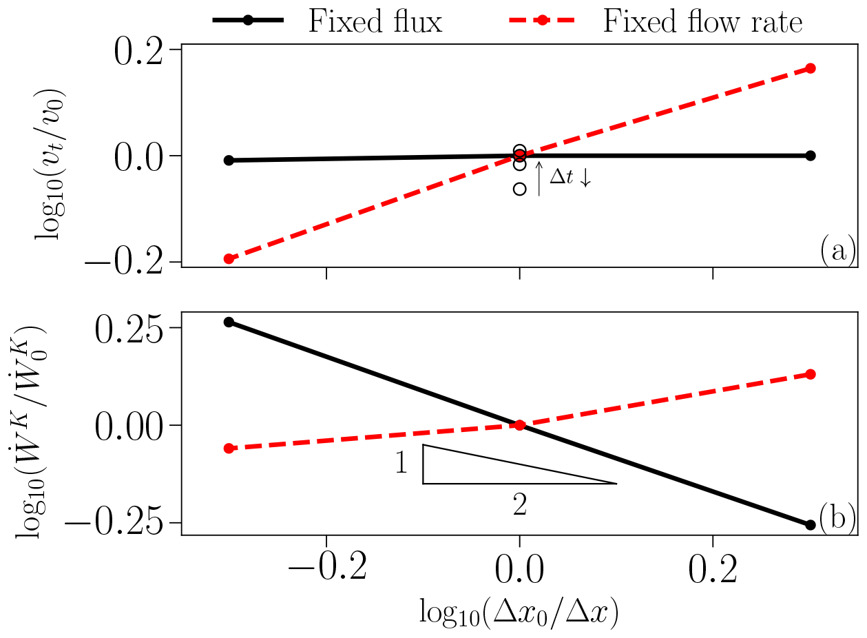
Figure E1 Mesh-dependency test for fixed-flux (solid black lines) and fixed-flow rate (dashed red lines) cases. The domain width is held constant while varying cell size of the mesh. (a) Variation of propagation speed (v_t) versus cell size (Δx). Solid circles represent variations in cell size with a fixed time step of Δt=0.5 years. Open circles that are aligned vertically represent variations in the time step (Δt=2, 1, 0.5, and 0.25 years, from bottom to top). Decreasing Δt values leads to an increase of v_t until a convergence is achieved, as indicated by the arrow. The reference case uses $\mathrm{\Delta }x=\mathrm{\Delta }z=\mathrm{40}$ m and Δt=0.5 years. (b) Variation of the viscoplastic dissipation rate (${\dot{W}}^{\mathrm{K}}$) versus cell size (Δx). The inset triangle illustrates the approximate power-law relationship, ${\dot{W}}^{\mathrm{K}}\sim \mathrm{\Delta }{x}^{\mathrm{1}/\mathrm{2}}$, for the fixed flux case (black line).

Figure E1a demonstrates convergence in propagation speed (v_t) with respect to decreasing time-step size (Δt). Reducing Δt from 0.5 to 0.25 years increases v_t by only approximately 2 %. Thus, Δt=0.5 years provides sufficient accuracy for the reference case.

Figure E1a further shows that propagation speed is independent of cell size when the flux ($Q_{\mathrm{0}}/\mathrm{\Delta }x$) is held constant rather than the flow rate (Q₀). This difference highlights a limitation of the current model: the dyke width cannot be smaller than the cell width.

Figure E1b indicates that the viscoplastic dissipation rate ${\dot{W}}^{\mathrm{K}}$ depends on cell size for both fixed flux and fixed flow rate conditions. For the fixed flux case, it follows an approximate power-law relationship, ${\dot{W}}^{\mathrm{K}}\propto \mathrm{\Delta }{x}^{\mathrm{1}/\mathrm{2}}$. Because the total dissipation rate is the integral of the local dissipation rate over the entire domain (Eq. 14), this dependency reinforces the model's limitation stated above. Note that Δz=Δx in these tests.

In summary, while the dyke propagation speed can be insensitive to grid spacing when fixing the liquid flux, the model requires further development for the viscoplastic dissipation rate to converge to a mesh-independent value.

Appendix F: Stress distribution of the (poro-)LEFM model

The stress distribution at the tip of the poro-LEFM model is identical to the mode-I fracture of the LEFM model,

$$\begin{array}{}\text{(F1)}& \left\{\begin{array}{c}{\mathit{\sigma }}_{xx}\\ {\mathit{\sigma }}_{zz}\\ {\mathit{\sigma }}_{xz}\end{array}\right\}={\displaystyle \frac{K_{\mathrm{c}}}{\sqrt{\mathrm{2}\mathit{\pi }r}}}\left\{\begin{array}{c}\cos (\mathit{\vartheta }/\mathrm{2})[\mathrm{1}-\sin (\mathit{\vartheta }/\mathrm{2}\left)\sin \right(\mathrm{3}\mathit{\vartheta }/\mathrm{2}\left)\right]\\ \cos (\mathit{\vartheta }/\mathrm{2})[\mathrm{1}+\sin (\mathit{\vartheta }/\mathrm{2}\left)\sin \right(\mathrm{3}\mathit{\vartheta }/\mathrm{2}\left)\right]\\ \sin (\mathit{\vartheta }/\mathrm{2})\cos (\mathit{\vartheta }/\mathrm{2})\cos (\mathrm{3}\mathit{\vartheta }/\mathrm{2})\end{array}\right\},\end{array}$$

where r and ϑ are the polar coordinates from the fracture tip, as shown in Fig. 5a. This formulation has also been used in Li et al. (2023).

Appendix G: Stresses and pressure inside of the dyke

This section discusses the differences in stresses and pressure inside the dyke between the poro-VEVP and poro-LEFM models. Taking p^l (liquid pressure) at the tail as an example, we have p^l=0 and $\partial p^{\mathrm{l}}/\partial z=\mathrm{0}$ in the poro-LEFM model but non-zero values for both in the poro-VEVP model. These differences stem from the nature of geometry and the complexity of stress balances.

Firstly, the poro-LEFM model assumes an infinitely long dyke, while the poro-VEVP model cannot make such an assumption. Consequently, the far-field condition of zero pressure and pressure gradient can be applied directly to the poro-LEFM model but not to the poro-VEVP model.

Secondly, the stress balance in the poro-LEFM model is simpler than in the poro-VEVP model. The poro-LEFM model assumes p^l=p^s and takes p^s as an elastic stress of the solid phase under one-dimensional deformation, as shown in Eq. (A7). However, the poro-VEVP model has a two-dimensional force-balance equation involving the gradient of tensor-form solid stresses and an extra term of static pressure gradient ϕΔρg, as shown in Eq. (6).

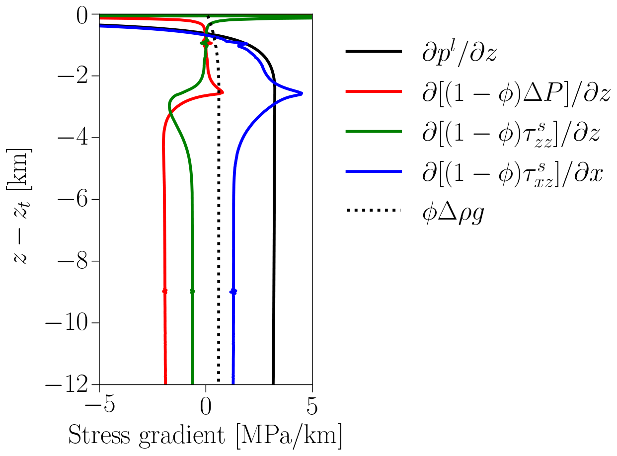
This complexity is evident in the force-balance equation along the dyke, which is the z-component of Eq. (6),

$$\begin{array}{}\text{(G1)}& \begin{array}{rl}-{\displaystyle \frac{\partial p^{\mathrm{l}}}{\partial z}}& +{\displaystyle \frac{\partial }{\partial x}}\left[(\mathrm{1}-\mathit{\varphi }){\mathit{\tau }}_{xz}^{\mathrm{s}}\right]+{\displaystyle \frac{\partial }{\partial z}}\left[(\mathrm{1}-\mathit{\varphi }){\mathit{\tau }}_{zz}^{\mathrm{s}}\right]\\ & -{\displaystyle \frac{\partial }{\partial z}}\left[\right(\mathrm{1}-\mathit{\varphi }\left)\mathrm{\Delta }P\right]+\mathit{\varphi }\mathrm{\Delta }\mathit{\rho }g=\mathrm{0}.\end{array}\end{array}$$

Here, ${\mathit{\tau }}_{xz}^{\mathrm{s}}$ and ${\mathit{\tau }}_{zz}^{\mathrm{s}}$ are components of the tensor-form solid deviatoric stresses, and ΔP is the compaction stress. These stresses are associated with deformation in both x and z directions. Even assuming no solid deformation, we have $\partial p^{\mathrm{l}}/\partial z=\mathit{\varphi }\mathrm{\Delta }\mathit{\rho }g$, where liquid pressure balances with static pressure. In general, none of the terms in the equation can be eliminated through scaling analysis.

Figure G1 shows numerical results of the vertical distribution for all five terms in the equation above for the reference case at t=2 kyr. Sufficiently far from the tip, all terms become invariant with respect to their vertical position, and none can be considered zero. Therefore, p^l is coupled with the gradient of full tensor-form stresses of the solid phase and thus also the full tensor-form strain rates. These values can only be determined through numerical computation, preventing us from prescribing boundary conditions consistent with the supposed stress gradient in the tail. This unavoidable difference leads to a boundary layer at the bottom serving as a transition in the numerical results, as shown in Fig. 3b and c.

Figure G1 Components of vertical stress gradients of the reference case at t=2 kyr.

Hence, quantitatively comparing stresses inside the dyke between the poro-VEVP and poro-LEFM models may not be reasonable, as evidenced by the mismatch in the grey region in Fig. 5b. However, we can compare stresses in the zero-porosity region outside the dyke (Fig. 5), where both models describe a two-dimensional elastic-stress distribution associated with the tip fracture. The poro-LEFM model's 2D stress field components are shown in Eq. (F1), representing a toughness-dominated distribution. The poro-VEVP model's components are computed numerically, with the dominant rheology being elasticity and the strong plastic deformation at the tip qualitatively similar to a discrete fracture. This intense plastic deformation is seen as the abrupt peak of plastic dissipation energy in Fig. 3d.

We also observe similarity in the porosity distribution inside the dyke near the tip (Fig. 4e), implying similar $\partial p^{\mathrm{l}}/\partial z$ near the tip due to Darcy's equation. Figure G1 shows $\partial p^{\mathrm{l}}/\partial z$ can be a leading term in the force-balance equation near the tip, suggesting similar fracture-dominated deformation despite different far-field stresses in the poro-VEVP dyke.