Linear Meta-Model optimization for regional climate models (LiMMo version 1.0)

A new tool for objective parameter tuning of regional climate models is presented. The climate model output was emulated using a linear regression approach for each grid point on a monthly mean basis. This linear approximation showed decent accuracy over a 6-year period. The root-mean-square error norm between the Meta-Model and the observational data sets was minimized using the gradient-based, limited-memory Broyden–Fletcher–Goldfarb–Shanno method with box constraints. We refer to this framework as LiMMo (Linear Meta-Model optimization). The LiMMo framework was applied to the state-of-the-art regional climate model ICON-CLM, tuned to the E-OBS and HOAPS observational data sets. Different optimization objectives were explored by assigning varying weights to model variables in the error norm definition. The combination of a linear emulator with fast gradient-based optimization allows the proposed method to scale linearly with the number of model variables and parameters, facilitating the tuning of dozens of parameters simultaneously.

1 Introduction

Tuning model parameters is crucial in Earth system modeling, where the aim is to minimize discrepancies between simulation results and observations. This process is essential for achieving reliable simulations in a variety of applications, ranging from short-term numerical weather prediction (e.g., Zängl, 2023) to long-term global and regional climate projections (e.g., Mauritsen and Roeckner, 2020). As model complexity and resolution continue to grow, tuning becomes increasingly challenging due to the computational expense of each simulation, therefore the demand for robust, transparent and efficient tuning procedures has grown significantly. Effective tuning improves model fidelity and enhances trust in model outcomes for policy-relevant decision-making.

In the context of global and regional climate models, four primary approaches to tuning have emerged (Hourdin et al., 2017). The first and most widely used is expert tuning, where model developers or users manually adjust parameters based on empirical experience and trial-and-error procedures (e.g., Mauritsen et al., 2012; Golaz et al., 2013). A more systematic alternative is metamodel-based tuning, also known as objective calibration, where a computationally cheap surrogate parameterized model (emulator) is constructed to approximate the behavior of the full model (e.g., Neelin et al., 2010; Bellprat et al., 2012). Third, Bayesian frameworks explicitly incorporate observational uncertainty and prior knowledge to estimate probability distributions of parameter values (see Kennedy and O'Hagan, 2001; Hourdin et al., 2023). Lastly, resolution-linked hierarchical emulators combine outputs from low- and high-resolution models to reduce computational burden while retaining accuracy (Williamson et al., 2012). This study contributes to the second category – objective calibration – by introducing a novel framework called LiMMo (Linear Meta-Model optimization), which employs a cost-efficient linear regression-based emulator combined with gradient-based optimization.

Previous studies on objective calibration have mainly centred on quadratic regression-based emulators, which permit nonlinear interactions among parameters and offer robust approximations (introduced in Neelin et al., 2010 and utilized in Bellprat et al., 2012, 2015; Avgoustoglou et al., 2022). However, a key limitation of this method is its high computational cost: the number of simulations required increases with the number of parameters (N) as N², since the simulation must be conducted for each pair of disturbed parameters in order to approximate interaction terms. To explore parameter space, many studies have employed Monte Carlo or Latin Hypercube sampling, which requires an exponentially growing number of samples to find global minimum for the error norm function, as dimensionality increases (Morokoff and Caflisch, 1995). Although this method is robust, it is computationally intensive and inefficient, restricting its use to tunings involving only a limited number of parameters – typically no more than seven. These constraints underscore the need for more efficient approximation and optimization approaches.

Another important issue is selecting an appropriate objective function to guide optimization. Although there are many alternatives, including multi-objective and probabilistic formulations, many studies continue to rely on simple metrics, such as root mean square error (RMSE) and/or Pearson correlation coefficient. However, RMSE and Pearson correlation may not capture all aspects of model performance (Liemohn et al., 2021). Nevertheless, to demonstrate the capabilities of the proposed LiMMo framework in a transparent and tractable way, this study focuses on minimizing RMSE. This relatively simple error norm allows us to demonstrate the LiMMo framework's capabilities, laying the groundwork for future expansions to more advanced metrics that take the distribution function into account.

The literature on statistical emulators includes Gaussian process models (Kennedy and O'Hagan, 2001; Williamson et al., 2013), high degree polynomial meta-models (Neelin et al., 2010; Bellprat et al., 2012), and hierarchical emulators that leverage multi-resolution outputs (Williamson et al., 2012). Despite its simplicity, linear regression has received less attention, even though it offers substantial efficiency benefits. Furthermore, gradient-based optimization techniques have rarely been applied to climate model tuning, partly due to the difficulty of computing derivatives. Taking advantage of the structural simplicity of linear regression makes it easier to derive the gradients of the objective function analytically and implement the gradient-based optimization procedure. This improves the scalability and convergence properties of the optimization process. To our knowledge, this is the first application of gradient-based optimization in the context of objective calibration for a regional climate model.

The following text is divided into five sections. The materials (Sect. 2) describes the tuned model quantities, the observational data sets, the regional climate model and its physical parameterizations. The tuning method is introduced in section The LiMMo framework (Sect. 3). The results of the optimization are presented in Sect. 4. Discussion in Sect. 5 covers aspects of tuning that fall outside the scope of the current study. Finally, the most important results are highlighted in conclusions (Sect. 6).

2 Materials

In this section, we provide a detailed description of ICON-CLM regional climate model (Pham et al., 2021). The model was configured at a 12 km spatial resolution over the EURO-CORDEX domain (Jacob et al., 2014) and optimized against observational data. The list of considered model quantities is presented in Sect. 2.1. Details of the observational data sets are provided in Sect. 2.2. The setup of the regional climate model ICON-CLM is described in Sect. 2.3, while the list of ICON-CLM tuning parameters is outlined in Sect. 2.4.

2.1 Model quantities

The list of surface prognostic variables (or model quantities) considered in this study is shown in the Table 1.

Table 1 The list of surface model quantities considered in the tuning process.

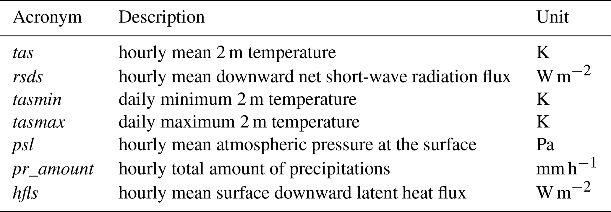
The selection of variables can be adjusted according to the user's interests. In addition to the commonly analyzed variables (tas, tasmin, tasmax, pr_amount, psl), we include the latent heat flux (hfls) due to its significant influence on long-term precipitation formation via evaporation over the sea. These 2D quantities were extracted from both climate model output and observational data sets for the tuning period from 1 January 2003 to 31 December 2008.

2.2 Observational data sets

The E-OBS version 29.0 data set (Cornes et al., 2018) was selected as a reference for tas, rsds, tasmin, tasmax, psl and pr_amount. This land-only, station-based observational gridded data set is compiled from high-density in-situ measurements provided by over 2000 European meteorological and hydrological stations. These measurements are then interpolated onto a regular grid and provided with ensemble uncertainty estimates. It provides high-quality daily data over Europe with a spatial resolution of approximately 25 km (12 km resolution is also available in the latest versions) and temporal coverage since 1950. Due to its fine spatial detail, daily temporal resolution and ensemble-based uncertainty estimates, E-OBS is a robust resource for analysing regional climate variability and long-term trends, and for making reliable climate assessments.

Our aim is to calibrate the hfls to align with the HOAPS version 4.0 data set (Andersson et al., 2010). HOAPS provides a satellite-based climatology of latent heat flux over the global ice-free oceans, derived from recalibrated SSM/I and SSMIS sensor measurements. The data set covers the period from 1987 to 2014, has a spatial resolution of approximately 55 km, and provides 6-hourly averages. HOAPS uses the COARE bulk flux algorithm version 2.6a (Fairall et al., 2003), to provide accurate estimates, making it a key reference for ocean-atmosphere interaction studies and energy exchange assessments.

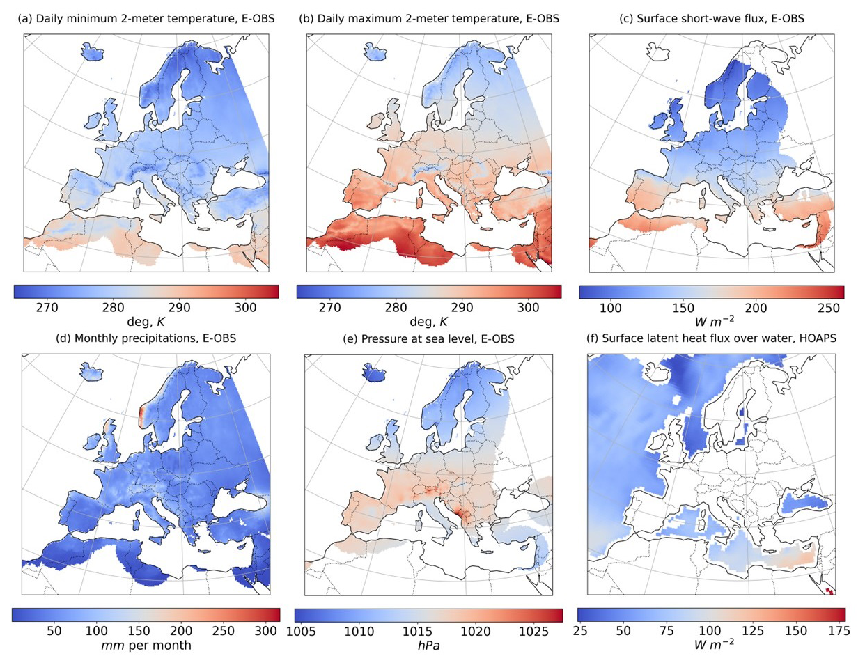
Figure 1 2003–2008 mean observations: (a) daily minimum 2 m temperature, E-OBS; (b) daily maximum 2 m temperature, E-OBS; (c) daily mean short-wave radiation flux, E-OBS; (d) total monthly precipitations, E-OBS; (e) daily mean atmostperic pressure at sea level, E-OBS; (f) daily mean latent heat flux over water, HOAPS.

Temporally averaged surface fields of tasmin, tasmax, rsds, pr_amount, psl, and hfls interpolated to the climate model output grid are shown in Fig. 1 for the tuning period 2003–2008.

2.3 Regional climate model ICON-CLM

ICON is a state-of-the-art model for global circulation modeling, Regional Climate Modeling (RCM), operational Numerical Weather Prediction (NWP), Large Eddy Simulations (LES), and environmental prediction (Zängl et al., 2015; Klocke et al., 2017; Stevens et al., 2017). The model is available since 2024. It uses an unstructured triangular grid, allowing nearly uniform resolution across the globe at any grid scale. The model is capable of simulations down to sub-kilometer scales, with common dynamics and numerics across all application modes. The model physics, however, differs between applications, with specific versions for Earth system modeling, NWP/RCM, and LES.

ICON-CLM (ICON in Climate Limited-area Mode) is the configuration used for RCM applications. It utilizes NWP physics with climate-specific extensions for long-term simulations. The first version of ICON-CLM is based on ICON release 2.6.1 (Pham et al., 2021). Typically, it operates in a one-way nesting mode, with coarse grid lateral boundary conditions and bottom boundary conditions over oceans. In the current study, Rayleigh damping is applied at the upper boundary to handle gravity waves.

The ICON release model version from July 2024 (ICON partnership (DWD, MPI-M, DKRZ, KIT, C2SM), 2024) is used with the ERA5 reanalysis (Hersbach et al., 2020) boundary conditions for the period 2003–2008. The simulation grid R13B5 (ICON terminology) corresponds to a mesh size of about 12.14 km. As a post-processing step, the model fields were interpolated onto a rotated 412×424 rectangular grid of the EURO-CORDEX model domain (Fig. 2) with a spatial resolution of 12 km, ensuring convenient data storage and accessibility for analysis.

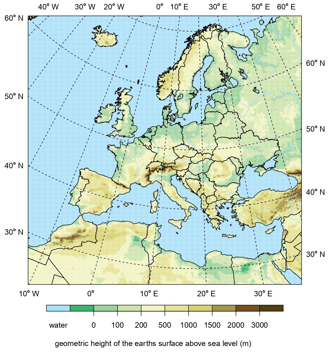
Figure 2 EURO-CORDEX domain, height of the Earths surface above sea level.

2.4 Tuning parameters of ICON-CLM

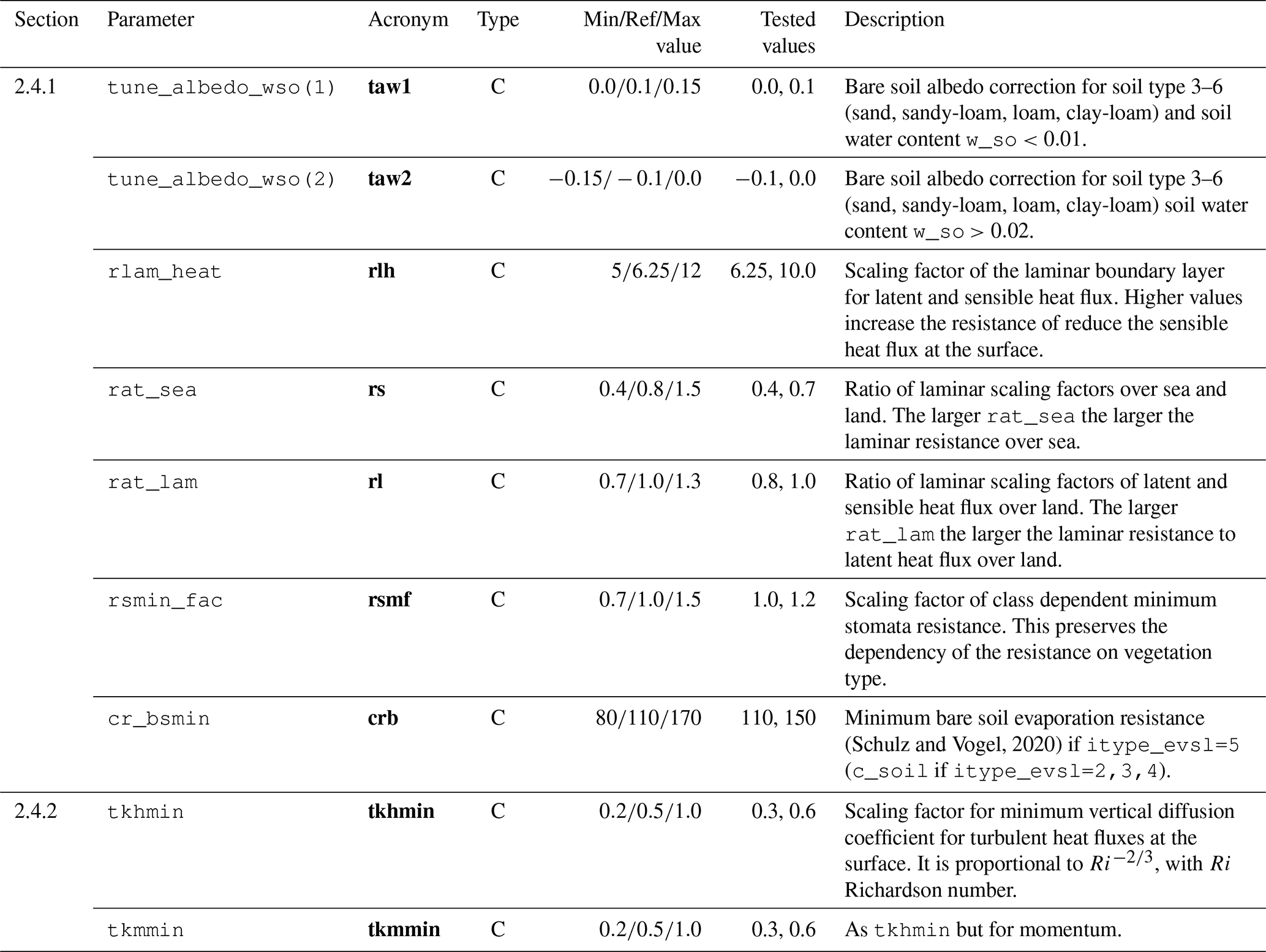
In this study, 15 parameters are selected for optimization, which is twice the number of parameters used in applications of the quadratic regression Meta-Model approach (Bellprat et al., 2012; Avgoustoglou et al., 2022). The following subsections discuss the physical meaning and relevance of these parameters. All model parameters are grouped into four categories. A brief description of the Surface Transfer Scheme (Sect. 2.4.1) and Mixing in the Planetary Boundary Layer (Sect. 2.4.2) parameters is given in Table A1. Descriptions of the Cloud Cover (Sect. 2.4.3) and External Data sets (Sect. 2.4.4) parameters can be found in Table A2. For more details, please refer to the ICON namelist parameter overview (https://gitlab.dkrz.de/icon/icon-model/-/blob/release-2024.07-public/doc/Namelist_overview.pdf, last access: February 2025).

The ICON namelist parameter names are designed to be self-explanatory, but this often results in them being quite long. To address this, the tables in the appendix (Tables A1 and A2) provide a mapping between the full ICON parameter names and the shorter versions used in the current study. In the text, ICON parameter names are highlighted with mono-space font, while the corresponding short acronyms are highlighted with bold font. For example, the ICON parameter for the relative humidity range is tune_box_liq, which corresponds to the acronym tbl.

2.4.1 Surface transfer scheme

The surface transfer scheme contains several tuning parameters, some of which are known to significantly impact near-surface climate conditions. These parameters, along with several related and newly introduced ones, are used for optimization. Specifically, the parameters rlam_heat, rat_sea, cr_bsmin, and rsmin_fac have been identified as particularly sensitive in climate modeling. Even small changes within their uncertainty ranges can lead to substantial changes in the simulated climate, particularly in the near-surface air temperature (tas). These parameters have been optimized in previous studies (Bellprat et al., 2012; Avgoustoglou et al., 2022).

The parameters rlam_heat and rat_sea, along with the newly introduced parameter rat_lam, serve to scale the resistance to latent and sensible heat flux over both land and sea surfaces, as described in the Table 2.

Table 2 Influence of the parameters rlam_heat, rat_sea, and rat_lam on the latent and sensible heat fluxes.

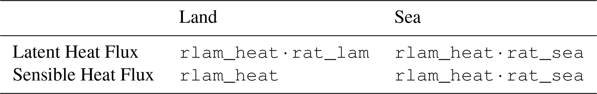
These parameters provide the flexibility to tune the heat fluxes over land and sea surfaces independently, and allow the adjustment of the Bowen ratio over land surfaces.

The parameters cr_bsmin and rsmin_fac represent the minimum resistance to evaporation from bare soil, relevant for wet soil conditions, and the scaling factor for the minimum resistance of plant transpiration, respectively. These minimum resistances limit evapotranspiration and are known to have a significant impact on soil moisture. Consequently, they influence the annual cycle climatologies, especially with respect to soil moisture dynamics.

Recently, the parameter pair $\mathtt{\text{tune\_albedo\_wso}}=(taw\mathrm{1},taw\mathrm{2})$ was introduced to correct the reference albedo for dry (taw1) and wet (taw2) soil conditions. This parameterization was initially motivated by the model's warm tas bias in the Mediterranean and cold bias in central and northern Europe. Additionally, it accounts for the fact that observed albedo tends to be reduced for wet soils and increased for very dry soils.

2.4.2 Mixing in the planetary boundary layer

The parameters tkhmin and tkmmin represent the minimum diffusion coefficients for vertical mixing of heat and momentum, respectively. They maintain mixing under opaque cloud cover and help dissolve the clouds, compensating for the excessive effective viscosity caused by numerical diffusion, which dampens instabilities. However, this minimum diffusion can keep mixing too high in stable, low-turbulence conditions, especially in winter, leading to excessively warm near-surface temperatures. These parameters should be as low as possible, but high enough to be effective, and have previously been optimized by expert judgment or objective calibration (Avgoustoglou et al., 2022). In this study, tkhmin and tkmmin are tuned simultaneously with the same factor (later the same acronym tkhmin is used for 𝚝𝚔𝚑𝚖𝚒𝚗=𝚝𝚔𝚖𝚖𝚒𝚗).

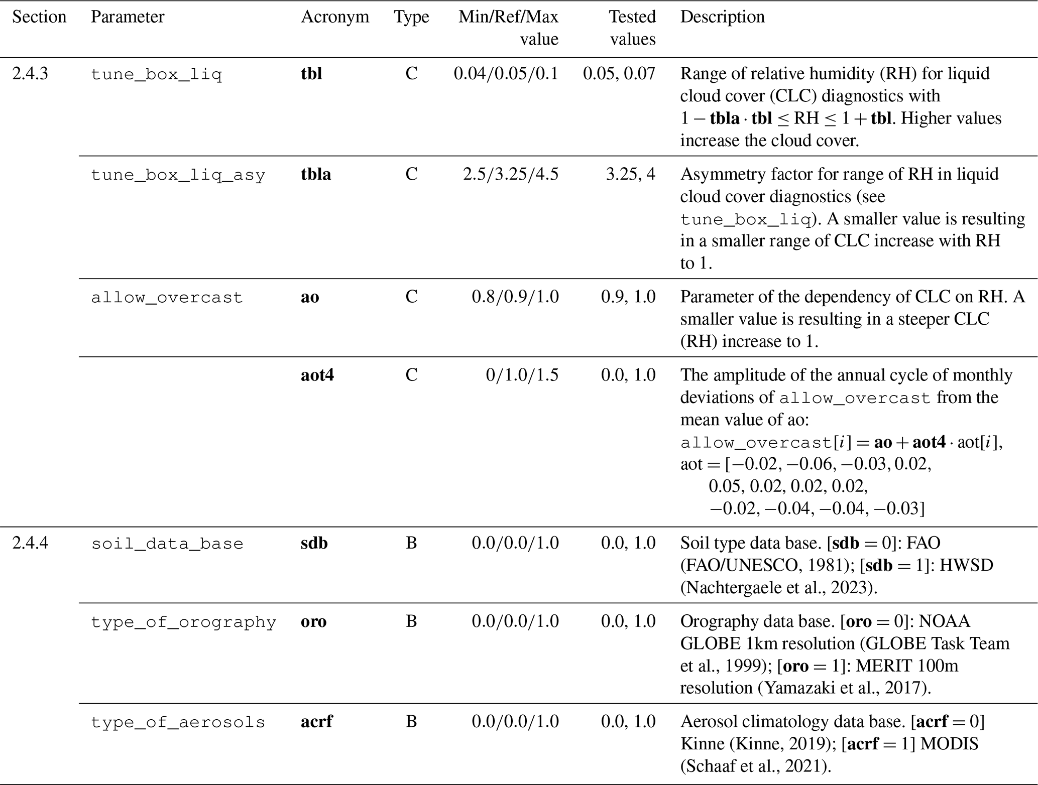
2.4.3 Cloud cover

The cloud cover parameters are optimized to address the rsds bias. The tune_box_liq and tune_box_liq_asy parameters are introduced to adjust the relationship between cloud cover (CLC) and relative humidity (RH), and are carefully tuned for operational NWP applications.

The allow_overcast factor further refines the dependence of cloud cover on relative humidity. Values less than one increase the average cloud cover. To incorporate seasonal variability, we define a time-dependent monthly variation for allow_overcast as follows:

$$\mathtt{\text{allow\_overcast}}\left[i\right]=\mathbf{ao}+\mathbf{aot}\mathbf{4}\cdot \mathrm{aot}\left[i\right],$$

where ao is the mean and aot[i] are the monthly deviations from that mean, i is the index of the month. The deviations are predefined to be positive in summer and negative in winter. This monthly variability is parameterized in the Meta-Model by the mean (ao) and the scaling factor ($\mathrm{0.0}\le \mathbf{aot}\mathbf{4}\le \mathrm{1.5}$) of the monthly deviations.

2.4.4 External data sets

In recent years, new data sets describing the physical properties of soils, surfaces, and the atmosphere have become available. In this study, we investigate the following alternative options:

• soil_data_base (sdb) describes the physical properties of the soil, provided by FAO (FAO/UNESCO, 1981) [sdb=0] and HWSD data (Nachtergaele et al., 2023) [sdb=1]. The FAO data set mainly represents sandy soils with a typical spatial resolution of 50 km, while the HWSD data set has a finer resolution of approximately 7 km.

• type_of_orography (oro) is used to calculate the grid-scale surface elevation and parameters required to parameterize subgrid-scale orographic effects. We use the global NOAA GLOBE data (GLOBE Task Team et al., 1999) [oro=0] with a resolution of 30 arcsec (approximately 1 km), or the Yamazaki-Lab MERIT data (Yamazaki et al., 2017) [oro=1] with a finer grid resolution of 3 arcsec (approximately 100 m).

• type_of_aerosols (acrf) parameterizes the feedback of the Cloud Condensation Nuclei Density (CDNC) on cloud formation. For this study, we use Kinne aerosol data (Kinne, 2019) [acrf=0], for which CDNC is not available, so we supplement it with MODIS (Schaaf et al., 2021) [acrf=1] CDNC data.

3 The LiMMo framework

This section introduces the LiMMo tuning framework. In principle, the described steps are model-independent, enabling users to adopt the framework for their own tuning objectives. The definition of the error norm relative to observations, which serves as the optimization objective, is discussed in Sect. 3.1. The Meta-Model approximation methodology is explained in Sect. 3.2. The proposed gradient-based optimization method is described in Sect. 3.3. Finally, in Sect. 3.4, we introduce the measure of variable sensitivities with respect to model parameters.

3.1 Error norm

The standard ICON-CLM model output is generated on an hourly basis (except for tasmin, tasmax which are daily). To reduce the temporal dimensionality, the daily means for tas, rsds, psl, and hfls and the daily sum for pr_amount are computed first. To maintain temporal consistency across analyses, an annual cycle of daily values was generated, based on multi-year daily means for each model variable. This approach allows for flexibility in the selection of time spans per variable to accommodate any temporal inconsistencies in observations. For this study, a uniform six-year period from 2003 to 2008 was used across all variables for both model outputs and observations to generate the annual cycle. In addition, to further reduce the dimensionality of the data, monthly mean values of the annual cycle were calculated for each model variable, consolidating the temporal dimension to 12. In principle, there is no need to accumulate the daily values first to generate the monthly averages of the annual cycles, since one can compute the monthly averages first and then compute the multi-year average of the annual cycle. However, this approach generally provides more flexibility, since it allows for more sophisticated distribution-based monthly quantities (e.g., 99th percentiles of hourly/daily values within climatological month).

To define the error norm we consider horizontal model results ${\mathrm{MOD}}_{i,j,k,n}$ for model variables v_n. The indices i, j correspond to horizontal surface spatial dimensions, k is the index of month. The observational data ${\mathrm{OBS}}_{i,j,k,n}$ were then interpolated to the model grid.

The spatially reduced Root Mean Square Error RMSE_k,n for each variable and time period is defined as

$$\begin{array}{}\text{(1)}& {\mathrm{RMSE}}_{k,n}=\sqrt{{\displaystyle \frac{\mathrm{1}}{N_x\cdot N_y}}\sum _{i,j}{\left({\mathrm{MOD}}_{i,j,k,n}-{\mathrm{OBS}}_{i,j,k,n}\right)}^{\mathrm{2}}},\end{array}$$

where N_x⋅N_y is the number of horizontal grid points of the simulation domain excluding the lateral boundary relaxation zone. For each variable and month the internal variability (or intrinsic uncertainty) σ_k,n is defined as the RMSE between the reference and disturbance simulation, where the initial conditions were shifted to 1 month

$$\begin{array}{}\text{(2)}& {\mathit{\sigma }}_{k,n}=\sqrt{{\displaystyle \frac{\mathrm{1}}{N_x\cdot N_y}}\sum _{i,j}{\left({\mathrm{MOD}}_{i,j,k,n}^{\mathrm{ref}}-{\mathrm{MOD}}_{i,j,k,n}^{\mathrm{dis}}\right)}^{\mathrm{2}}}.\end{array}$$

In order to obtain a reliable measure of the intrinsic uncertainty of the model, both the reference and disturbance simulations should cover a sufficiently long period, as is the case in the current study with a 6-year period. Otherwise, significant imbalances in the monthly values within the climatological year can occur. The unit less error ERR_n for each variable is defined as the averaged over months RMSE normalized on internal variability

$$\begin{array}{}\text{(3)}& {\mathrm{ERR}}_n={\displaystyle \frac{\mathrm{1}}{N_t}}\sum _k{\displaystyle \frac{{\mathrm{RMSE}}_{k,n}}{{\mathit{\sigma }}_{k,n}}},\end{array}$$

where N_t=12 is the number of months. The final error norm ERR is defined as the weighted sum of the errors for each variable

$$\begin{array}{}\text{(4)}& \mathrm{ERR}=\sum _n{c}_n\cdot {\mathrm{ERR}}_n,\sum _n{c}_n=\mathrm{1}.\end{array}$$

The weights c_n are specified by the user to emphasize the importance of a particular variable and should have the unit sum. The goal of the tuning process is to minimize the error norm (Eq. 4) with respect to the model parameters.

3.2 The linear meta-model approximation

The mean climate can be regarded as a balanced, stable stationary state and thus to be weakly dependent on the model parameters p_i. This allows to consider the climate state CLI as a function of a model parameter vector p and to expand CLI(p) in a Taylor series around the reference model solution CLI(p₀). The linear meta model is the first order approximation of the climate state:

$$\begin{array}{}\text{(5)}& \mathrm{CLI}\left(\mathit{p}\right)\approx \mathrm{CLI}\left({\mathit{p}}_{\mathrm{0}}\right)+{\mathrm{\nabla }}_{\mathit{p}}\mathrm{CLI}\left({\mathit{p}}_{\mathrm{0}}\right)\cdot \left(\mathit{p}-{\mathit{p}}_{\mathrm{0}}\right).\end{array}$$

We rewrite Eq. (5) in the form of a linear regression ${\mathrm{REG}}_{i,j,k,n}$ for each grid point (x_i, y_j), month m_k and variable v_n

$$\begin{array}{}\text{(6)}& {\mathrm{REG}}_{i,j,k,n}\left(\mathit{p}\right)=A_{i,j,k,n}+\sum _{m=\mathrm{1}}^{N_{\mathrm{c}}}{p}_m\cdot K_{i,j,k,n}^m,\end{array}$$

where $A_{i,j,k,n}$ is the shift tensor, $K_{i,j,k,n}^m$ is the tendency tensor (m is the index of the parameter) and N_c is the number of continuous parameters considered.

To train the linear regression model we present the analytical values of a tendency tensor $K_{i,j,k,n}^m$ for each m, obtained by the method of undefined coefficients by substituting simulations to the general form of linear regression (Eq. 6). After substituting the reference and single parameter disturbance simulation, the value of the tendency tensor is defined as the fraction of the simulation difference to the parameter increment. For example, one can obtain the tensor $K_{i,j,k,n}^m$ corresponding to the parameter p_m as

$$\begin{array}{}\text{(7)}& K_{i,j,k,n}^m={\displaystyle \frac{{\mathrm{MOD}}_{i,j,k,n}^{p_m=p_m^{\mathrm{ref}}+\mathrm{\Delta }{p}_m}-{\mathrm{MOD}}_{i,j,k,n}^{p_m=p_m^{\mathrm{ref}}}}{\mathrm{\Delta }{p}_m}},\end{array}$$

since the other parameters except p_m remained unchanged. If more than one linear combination could define the tendency on the parameter, the least-square technique is utilized. The specific values of the parameters used for training (tested values) can be found in Tables A1 and A2. After the computation of all tendency tensors, the additional substitution of the reference simulation gives the value of the shift tensor

$$\begin{array}{}\text{(8)}& A_{i,j,k,n}={\mathrm{MOD}}_{i,j,k,n}^{\mathrm{ref}}-\sum _{m=\mathrm{1}}^{N_{\mathrm{c}}}{p}_m^{\mathrm{ref}}\cdot K_{i,j,k,n}^m.\end{array}$$

To account for logical switches, we incorporate constant signals into the Meta-Model (Eq. 6):

$$\begin{array}{}\text{(9)}& \begin{array}{rl}{\mathrm{REG}}_{i,j,k,n}\left(\mathit{p}\right)& =A_{i,j,k,n}+\sum _{m=\mathrm{1}}^{N_{\mathrm{c}}}{p}_m\cdot K_{i,j,k,n}^m+\sum _{l=\mathrm{1}}^{N_{\mathrm{b}}}{p}_l\\ & \cdot \left({\mathrm{MOD}}_{i,j,k,n}^{p_l=\mathrm{1}}-{\mathrm{MOD}}_{i,j,k,n}^{p_l=\mathrm{0}}\right),\end{array}\end{array}$$

where N_b denotes the number of binary (logical) parameters, and each binary parameter p_l can take the values 0 or 1. The reference simulation assumes p_l=0 for all binary parameters. When p_l=0, the logical switch is off, and no additional signal is added, so the Meta-Model would reproduce the state of the reference simulation. The inclusion of binary parameters introduces constant shifts in the emulator, but does not affect the gradient of the Meta-Model with respect to continuous parameters. Consequently, the following minimization involves only continuous parameters, while logical ones are prescribed to 0 or 1.

3.3 The gradient-based optimization

The core concept behind Meta-Model tuning is to replace the climate model output with a regression approximation in the definition of the error norm (Eq. 4). Due to the simplicity of the Meta-Model, the gradient of the error norm with respect to the model parameters can be computed analytically. The linear regression approximation (Eq. 9) provides the following analytical expression for the gradient with respect to the continuous parameters:

$$\begin{array}{}\text{(10)}& {\left({\displaystyle \frac{\partial \mathrm{REG}}{\partial \mathit{p}}}\right)}_m=K_{i,j,k,n}^m.\end{array}$$

Using the chain rule, the analytical form of the gradient of the error norm (Eq. 4) could be written as

$$\begin{array}{}\text{(11)}& \begin{array}{rl}{\left({\displaystyle \frac{\partial \mathrm{ERR}}{\partial \mathit{p}}}\right)}_m& =\sum _n{c}_n{\displaystyle \frac{\mathrm{1}}{N_t\cdot N_x\cdot N_y}}\sum _k{\displaystyle \frac{\mathrm{1}}{{\mathit{\sigma }}_{k,n}\cdot {\mathrm{RMSE}}_{k,n}\left(\mathit{p}\right)}}\\ & \cdot \sum _{i,j}\left({\mathrm{REG}}_{i,j,k,n}\left(\mathit{p}\right)-{\mathrm{OBS}}_{i,j,k,n}\right)\cdot K_{i,j,k,n}^m.\end{array}\end{array}$$

The computation of the gradient requires one loop over grid points (i, j), time (k), and model variables (n), making its duration comparable to that of a single norm evaluation $O(N_x\cdot N_y\cdot N_t\cdot N_{\mathrm{vars}})$.

The availability of a fast gradient computation procedure allows the use of different optimization methods. Gradient-descent-type optimization involves iterations over the vector of parameters p that search for the minimum error norm function (Eq. 4) in the direction opposite the gradient (Eq. 11).

This study proposes the implementation of the Limited-memory Broyden–Fletcher–Goldfarb–Shanno with Box constraints (L-BFGS-B) algorithm (Broyden, 1970; Byrd et al., 1995). This method is chosen due to its high convergence speed, being a quasi-Newton method that approximates the Hessian matrix, and its capability to impose constraints on parameter ranges, thereby eliminating nonphysical parameter values during the optimization.

In gradient-based optimization, parameter normalization is highly beneficial, as it results in a spherical shape of isolines, improving the convergence rate by avoiding the steep slopes of the objective function

$$\begin{array}{}\text{(12)}& p_i^{\mathrm{new}}={\displaystyle \frac{p_i^{\mathrm{old}}-p_i^{\min }}{p_i^{\max }-p_i^{\min }}}.\end{array}$$

The parameter ranges $p_i^{\min }/p_i^{\max }$ are user-defined (Tables A1 and A2) and are used for parameter normalization as well as for the box constraints in L-BFGS-B optimization. Applying this linear transformation to the parameters results in the following transformation of the gradient function

$$\begin{array}{ll}{\displaystyle }{\left({\displaystyle \frac{\partial }{\partial \mathit{p}}}f\left(p_{\mathrm{1}}^{\mathrm{new}},\mathrm{\dots },p_m^{\mathrm{new}}\right)\right)}_i& {\displaystyle }=\left(p_i^{\max }-p_i^{\min }\right)\\ {\displaystyle }& {\displaystyle }\cdot {\left({\displaystyle \frac{\partial }{\partial \mathit{p}}}f\left(p_{\mathrm{1}}^{\mathrm{old}},\mathrm{\dots },p_m^{\mathrm{old}}\right)\right)}_i.\end{array}$$

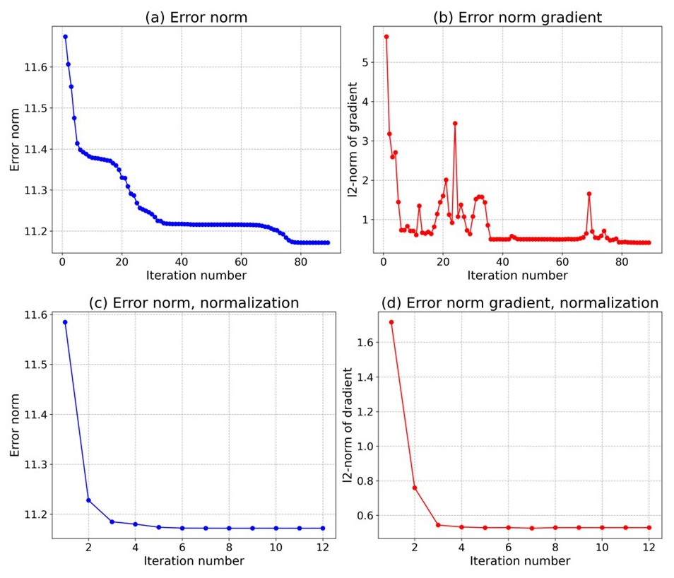
Figure 3 illustrates the difference in convergence of the proposed method with and without parameter normalization for a specific parameter configuration. The results clearly demonstrate that the normalized approach achieves the same objective function value, but with an order of magnitude fewer iterations (the objective function decrement was set to 10⁻⁵ as the stop criterion in both cases).

Figure 3 Convergence of L-BFGS-B method: error norm (Eq. 4) values without (a) and with (c) parameter normalization, l2-norm of error norm gradient (Eq. 11) without (b) and with (d) parameter normalization.

The dependence of the solution on the initial conditions can lead to different optimization results. An extremely high optimization speed makes it possible to consider the ensemble of optimization trajectories with the perturbed initial conditions. We propose to select the perturbed initial conditions from the Latin Hypercube vicinity of the reference parameters

$$\begin{array}{}\text{(13)}& \begin{array}{rl}\left[p_m^{\mathrm{ref}}-\mathrm{AMPL}\right.& \cdot \left(p_m^{\max }-p_m^{\min }\right),p_m^{\mathrm{ref}}+\mathrm{AMPL}\\ & \left.\cdot \left(p_m^{\max }-p_m^{\min }\right)\right],m=\stackrel{\mathrm{‾}}{\mathrm{1},N_{\mathrm{c}}}.\end{array}\end{array}$$

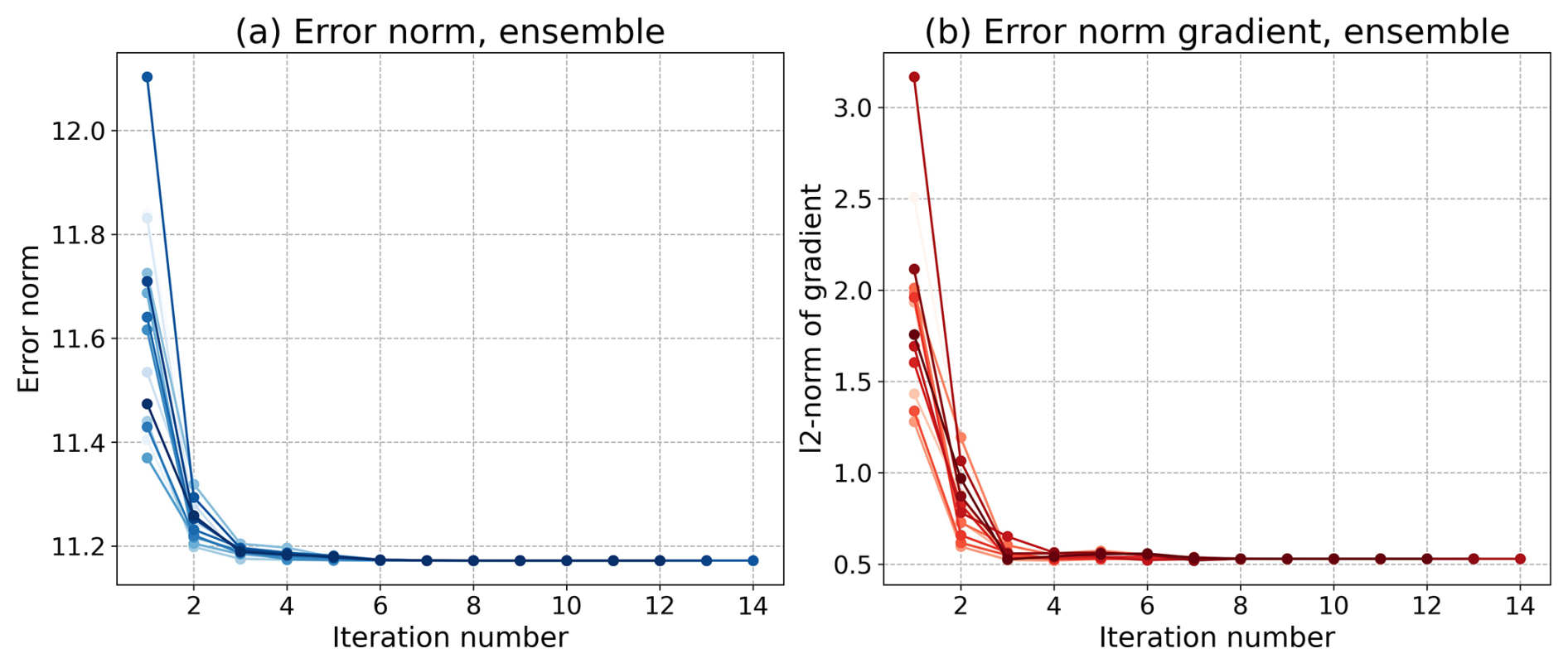
The scaling factor $\mathrm{AMPL}\in [\mathrm{0},\mathrm{1}]$ defines the amplitude of the perturbation. In the case of the linear regression emulator with a simple RMSE score function, we found no dependence of the result on the initial conditions, as shown in Fig. 4 (we used AMPL=0.3 and 15 samples), but this may be different for more advanced statistical emulators or error norm definitions. If a dependence on the initial conditions occurs, one could choose the result with the minimum value of the objective function.

Figure 4 The axes are the same as in Fig. 3. Ensemble of 15 optimization trajectories with disturbed initial conditions: (a) error norm (Eq. 4), (b) l2-norm of error norm gradient (Eq. 11).

Gradient-based optimization with an analytical representation of the gradient is highly advantageous in terms of performance. The use of linear regression as the statistical emulator results in a linear scaling of the dimensions of the problem (number of variables, parameters, grid points, and time steps), allowing a large number of parameters to be tuned in a reasonable amount of time. A numerical approximation of the gradient is also possible in the case of a more sophisticated statistical emulator or an error norm definition, when the analytical expression is unavailable.

3.4 Sensitivity measure

To estimate the sensitivity of the ICON-CLM and consequently of the regression model to the considered parameters, the unit-less measure of maximum change SENS_n,m is calculated for each prognostic variable. Firstly we compute the maximal function increments by separately changing all parameters to their limits

$$\begin{array}{}\text{(14)}& \begin{array}{rl}\mathrm{\Delta }& {\mathrm{REG}}_{i,j,k,n}^{m,\min /\max }={\mathrm{REG}}_{i,j,k,n}\left(p_{\mathrm{1}}^{\mathrm{ref}},\mathrm{\dots },p_m^{\min /\max },\mathrm{\dots },\right.\\ & \left.p_{N_{\mathrm{p}}}^{\mathrm{ref}}\right)-{\mathrm{REG}}_{i,j,k,n}\left(p_{\mathrm{1}}^{\mathrm{ref}},\mathrm{\dots },p_m^{\mathrm{ref}},\mathrm{\dots },p_{N_{\mathrm{p}}}^{\mathrm{ref}}\right),\end{array}\end{array}$$

where N_p is the total number of parameters, including continuous and logical ones. Here, $\mathrm{\Delta }{\mathrm{REG}}_{i,j,k,n}^{m,\min }$ is the regression increment where only the parameter p_m is changed to its minimum limit. Similarly $\mathrm{\Delta }{\mathrm{REG}}_{i,j,k,n}^{m,\max }$ corresponds to the regression increment when p_m is changed to its maximum. The sensitivity benchmark SENS_n,m of the variable v_n to the parameter p_m is defined as the maximum of the sensitivities revealed for $p_m=p_m^{\min }$ and $p_m=p_m^{\max }$ respectively

$$\begin{array}{}\text{(15)}& {\mathrm{SENS}}_{n,m}=\max \left({\mathrm{SENS}}_{n,m}^{\min },{\mathrm{SENS}}_{n,m}^{\max }\right).\end{array}$$

Equation (16) gives the expression for calculating the ${\mathrm{SENS}}_{n,m}^{\min }$ and ${\mathrm{SENS}}_{n,m}^{\max }$ as the monthly mean signal-to-noise measures (normalized by internal variability σ_k,n) of regression increment where $p_m=p_m^{\min }$ and $p_m=p_m^{\max }$ respectively (Eq. 14)

$$\begin{array}{}\text{(16)}& \begin{array}{rl}{\mathrm{SENS}}_{n,m}^{\min /\max }& ={\displaystyle \frac{\mathrm{1}}{N_T}}\cdot \sum _k{\displaystyle \frac{\mathrm{1}}{{\mathit{\sigma }}_{k,n}}}\\ & \cdot \sqrt{{\displaystyle \frac{\mathrm{1}}{N_x\cdot N_y}}\cdot \sum _{i,j}{\left(\mathrm{\Delta }{\mathrm{REG}}_{i,j,k,n}^{m,\min /\max }\right)}^{\mathrm{2}}}.\end{array}\end{array}$$

4 Results

In this section, we analyze the sensitivity results (Sect. 4.1) and the regression validation (Sect. 4.2) to identify the most influential parameters and to evaluate the performance of the proposed statistical emulator. Subsequently, an example application of LiMMo is presented for a selected parameter set (Sect. 4.3), demonstrating its flexibility in handling varying variable weights. Additionally, the results of an optimization incorporating logical switches (Sect. 4.4) constraints are discussed.

4.1 Sensitivity results

The sensitivity measures for all parameters computed as Eq. (15) are shown in Fig. 5.

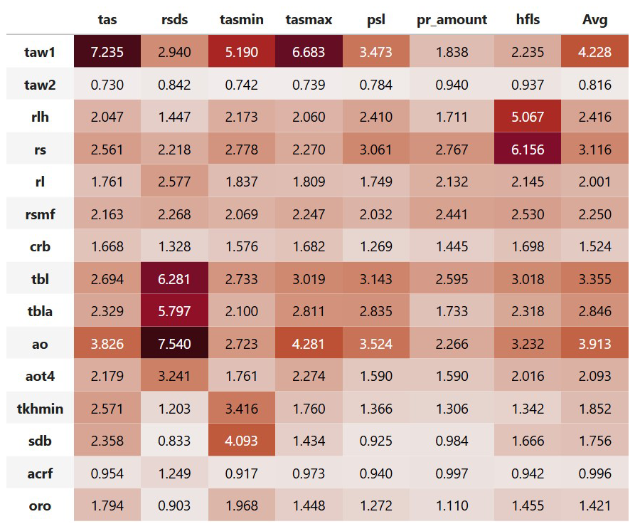
Figure 5 The sensitivity measure of prognostic variables (columns) on model parameters (rows) computed as Eq. (15). The “Avg” column shows the mean sensitivity of the model to the parameter, calculated as the mean values in the rows. Darker shades are used to color the background of the numbers for larger values.

Overall, the sensitivity results are consistent with theoretical expectations. It is clear that the surface albedo parameterisation taw1 is the primary driver of surface air temperature variations (tas, tasmin, tasmax). taw2 has a negligible impact on the model variables, which is below the level of the ICON-CLM's intrinsic variability. The heat flux scaling factors rlh and rs show sensitivity primarily to latent heat flux over the sea (hfls), with a moderate impact on other quantities. The ratio of the laminar scaling factors rl has the greatest impact on short-wave radiation (rsds), contributing only slightly to precipitation (pr_amount) and latent heat flux (hfls). The soil resistance parameters rsmf and crb exhibit sensitivity across all model variables. Although optimizing these parameters may not lead to improvements in one variable without affecting others, their inclusion may still be beneficial for optimization.

The cloud cover parameters tbl and tbla and the allow overcast parameters ao and aot4 demonstrate the most pronounced sensitivity to short-wave radiation (rsds), as expected. The momentum and vertical diffusion coefficient tkhmin primarily influence the mean (tas) and the minimum (tasmin) daily temperatures with minimal impact on other variables, suggesting opportunities for targeted tuning.

The external soil database sdb primarily affects the mean (tas) and the minimum (tasmin) daily temperature. Aerosol type acrf has only a limited effect on short-wave radiation (rsds). The orography type oro has a small effect on all model variables, although it is known to influence wind speed, which is outside the scope of this study.

The proposed sensitivity measure is highly effective for evaluating the impact of parameter changes on model variables and for comparing these impacts quantitatively. This analysis is particularly valuable when considering new parameters, as it helps to assess their influence on model results. Parameters that have a low sensitivity across all model variables (less than 1) could either be removed from the optimization or have the limits of their variation expanded.

4.2 Meta-model validation

Several parameter configurations were additionally simulated with ICON-CLM to evaluate the accuracy of the linear Meta-Model approximation. Due to limited computational resources, only a subset of parameters was considered. The most influential parameters, which exhibited the largest sensitivity in the sensitivity analysis (see Fig. 5), were selected: taw1, rlh, rs, rl, tbl, tbla, ao and tkhmin. Test samples were generated by simultaneously varying these parameters from the Latin Hypercube within the intervals from minimum to maximum values (see Tables A1 and A2).

A direct comparison between the regression model and the ICON-CLM simulation for different grid points and months is presented in Fig. 6. Here values are plotted together for all test cases from Latin Hypercube. For the variables tas, tasmin, tasmax, psl, and hfls, the coefficient of determination (R²) exceeds 0.95 (not shown), indicating a decent approximation by the linear model. The variable rsds exhibits some spread around the mean, but maintains a high determination coefficient (>0.99). The precipitation (pr_amount) shows the poorest performance of all optimization variables. The spread exhibits values of up to 100 mm per month and the determination coefficient R² is 0.9 only. A comparison of the histograms (not shown) reveals that the Meta-Model yields slightly higher precipitation values than ICON-CLM. Also, due to the lack of physical constraints, the Meta-Model yields marginally negative precipitation values; however, their impact on the overall RMSE is very limited (approximately 3 % of the intrinsic uncertainty of precipitation (Eq. 2)).

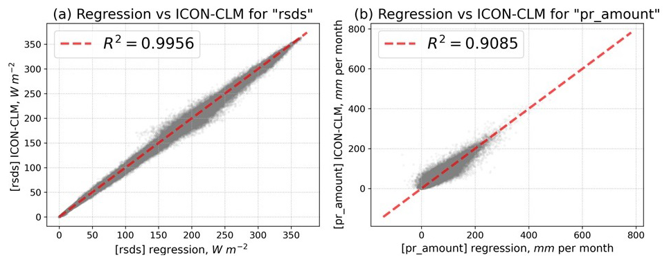
Figure 6 Regression vs. ICON-CLM for the variables rsds (a) and pr_amount (b). Each grey point shows the monthly value of the model quantity for a single grid point in the model domain, for one of the validation configurations (i.e., all validation cases plotted together). The dashed red line indicates “perfect match”, the value of the R² determination coefficient is given in the label. Every 100th grid point is shown in the plot.

To assess the inaccuracy of the approximation statistically, we computed the monthly mean values of RMSE between the ICON-CLM output and the linear Meta-Model for each test case in the Latin Hypercube, and plotted the mean values in Fig. 7. As can be seen, the imprecision of the linear approximation (green bars) is slightly greater than the intrinsic uncertainty of the ICON-CLM (orange bars), by a factor of 1.5–1.7 for tas, rsds, tasmin, tasmax and pr amount, and by a factor of 2.5 for hfls. However, this imprecision (green bars) is still much smaller than the typical error to observations (blue bars) for all variables except precipitation, indicating the potential for optimization.

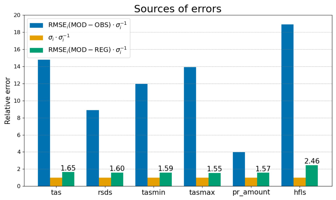
Figure 7 The comparison of the different sources of error in LiMMo. Values are normalized on the intrinsic variability σ_i of the ICON-CLM (Eq. 2) for each model variable. The blue bar shows the RMSE of the ICON-CLM output with the NWP configuration to the observations. The orange bar shows the intrinsic variability. The green bar shows the RMSE between the ICON-CLM and the linear regression approximation, averaged over all test cases from Latin Hypercube. The temporally averaged values (averaged for all months) are displayed for all quantities.

The linear approximation error for various variables was also assessed by comparing the time-averaged (averaged over all climatological months) RMSEs to the observations (Eq. 1), as shown in Fig. 8. For each of the Latin Hypercube validation setups, we plot the RMSE to observations for different pairs of variables, for both the linear regression approximation and the corresponding dynamical simulation. The scores of the dynamical simulations and their corresponding Meta-Model approximations are represented by markers of identical shape. With a few exceptions, the order of the RMSEs for the linear and dynamic models is largely maintained, i.e., if the RMSE is smaller for the regression results, the same is true for the dynamical simulation. This justifies the reduction in the RMSE-based error norm for the linear emulator, which is minimized by the optimization procedure, corresponding to an improved dynamic setup with reduced biases. This is particularly true when the reduction in RMSE exceeds the level of imprecision in the approximation, bearing in mind the error in the linear approximation.

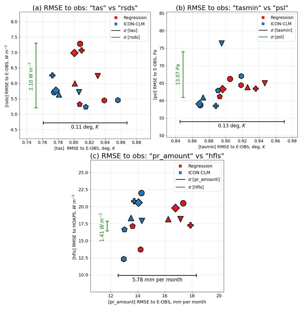
Figure 8 The monthly mean RMSEs (Eq. 1) to observations for ICON-CLM simulations (blue markers) and corresponding regression results (red markers) for all parameter setups from Latin Hypercube. Corresponding dynamical and linear setups are indicated by the same marker shape. The 2003–2008 monthly mean RMSEs are shown for: (a) daily mean 2 m temperature tas versus daily mean short-wave flux rsds, (b) daily minimum 2 m temperature tasmin versus daily mean sea level pressure psl, (c) monthly total precipitation pr_amount versus daily mean latent heat flux hfls. The 2003–2008 mean internal variabilities of the model (Eq. 2) are shown as horizontal and vertical segments.

This analysis demonstrates the applicability and reliability of the linear approach for representing the dynamical simulations.

4.3 Tuning of continuous parameters

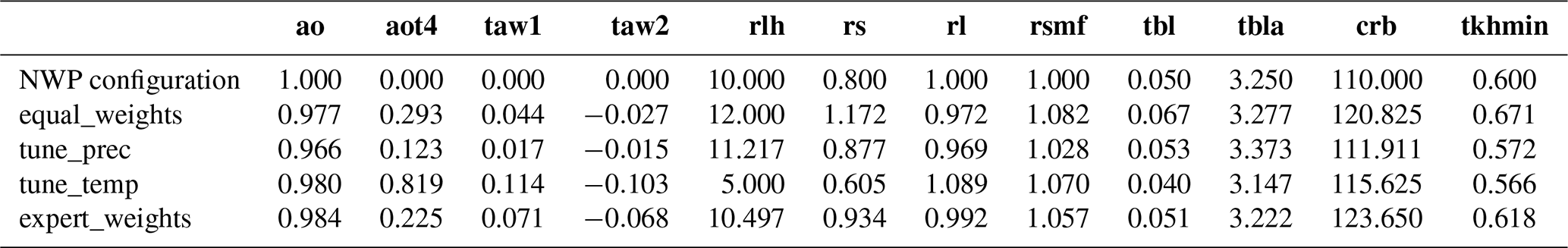
LiMMo provides substantial flexibility in the selection of regression parameters for optimization as well as in the weighting of model variables. To systematically evaluate its performance, we fix the set of continuous parameters to the following: ao, aot4, taw1, taw2, rlh, rs, rl, rsmf, tbl, tbla, crb, and tkhmin. Four different weight configurations (Table 3) for the model variables that define the error norm in Eq. (4) are analyzed. As the reference configuration, we used the proposed configuration of ICON for NWP, which defines the shift tensor in Eq. (8). The parameter values of the reference configuration can be found in Table 4.

Table 3 The list of considered weights in the error norn definition (Eq. 4). Each row represents the set of weights of the model quantities (columns).

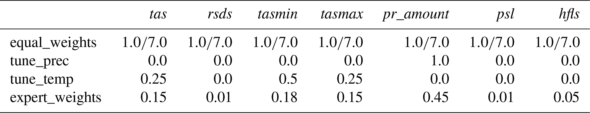
Table 4 The parameter values for the ICON-CLM for the NWP configuration and configurations obtained from LiMMo using different weights from Table 3. The rows of the table correspond to the different weights of the variables in the optimization, the columns represent the model parameters.

The first configuration, “equal_weights”, assigns equal weights to all model variables. LiMMo allows to explore the predictive potential of the climate model for specific fields, therefore, two extreme cases are considered: “tune_prec” assigns weights exclusively to precipitation, neglecting all other variables, while “tune_temp” distributes weights among tas, tasmin, and tasmax. Finally, the “expert_weights” configuration reflects weights determined a posteriori by the authors based on an analysis of the optimization results. There are also some objective ways of defining weights, such as entropy weights for multi-criteria decision-making in information theory, which are beyond the scope of the current study. These could be implemented in the LiMMo framework by assigning a variable weight that is inversely proportional to signal-to-noise values of the initial configuration for each model quantity.

The performance scores of the model variables (Eq. 3) after optimization are shown in Fig. 9. Note that in the current study we tend to minimize the variable scores (error norms), so the reduced score values demonstrate the better performance. It is evident that the predictability of precipitation is approaching its theoretical limit for the selected set of model parameters, as the optimal score of pr_amount in the “tune_prec” configuration is only slightly (∼2 %) lower than that of the reference configuration. It is also worth noting that the initial NWP configuration is already very well tuned for precipitation. Conversely, when optimizing only for temperature variables (“tune_temp”), significant error reductions are achievable: a 5 % reduction for tas, a 12 % reduction for tasmax, and a 4 % reduction for tasmin. However, this comes at the cost of a significant imbalance in the surface heat budget, with notable increases in rsds (5 %) and hfls (47 %). The quality of pr_amount is also badly affected by 15 %.

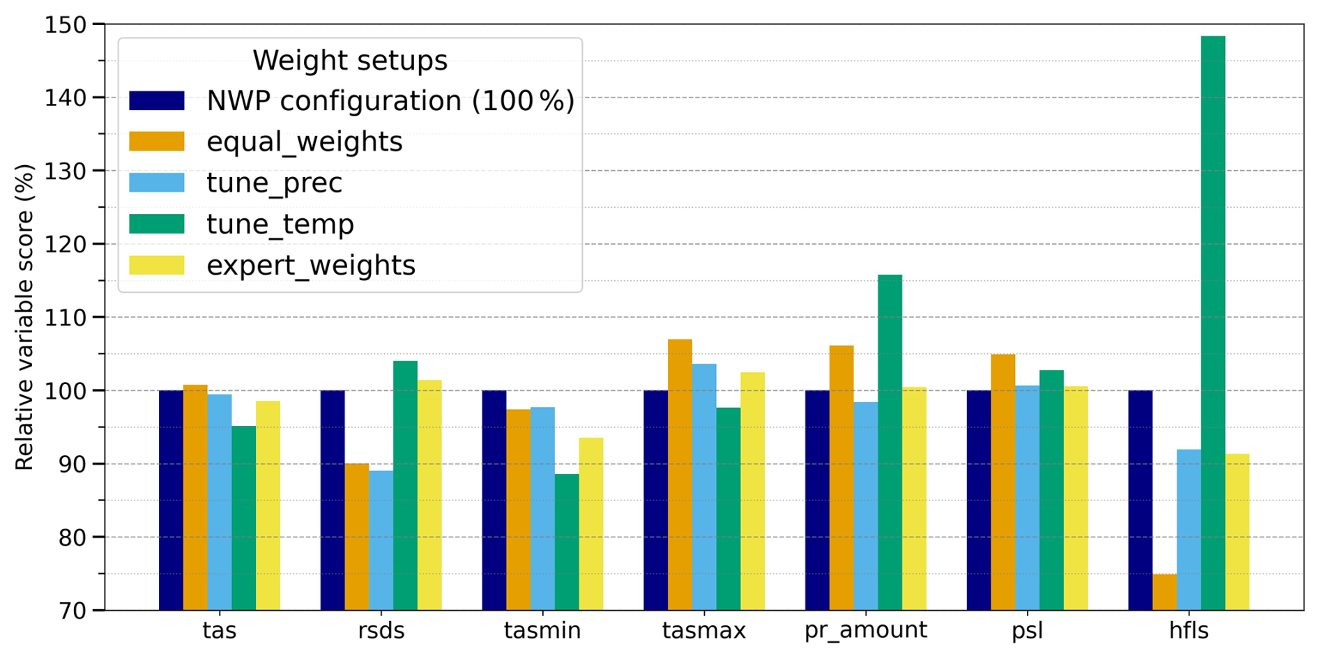
Figure 9 Scores of model variables (Eq. 3) normalized by the variable score of NWP configuration (dark blue bars) after optimization with different weights from Table 3. Note that in the current study we aim to minimize the variable scores (error norms), so the reduced score values demonstrate the better performance.

The “equal_weights” setup demonstrates significant reductions in rsds (10 %) and hfls (25 %), but it underperforms the NWP configuration for the key prognostic variables tas, tasmax, and pr_amount. On the other hand, the “expert_weights” setup achieves comparable performance to the NWP configuration for most variables, with the exception of rsds (1 %–2 % worse) and tasmax (2 %–3 % worse). In particular, this setup yields significant improvements in the values of tasmin (7 %) and hfls (∼10 %). Consequently, the “expert_weights” setup can be considered as a viable alternative to the NWP configuration. The optimal values of the considered parameters are listed in the Table 4.

4.4 Optimization with logical switches

This subsection presents the optimization results obtained using the Meta-Model with incorporated logical switches (Eq. 9). The parameter set is fixed as in the previous subsection, with the “expert_weights” weight configuration applied. The study considers three logical parameters (sdb, acrf and oro), resulting in a total of eight possible optimizations. The continuous parameters were optimized for each configuration of logical switches that defines the shifted linear Meta-Model. The results are summarized in Fig. 10. This final scores table provides the comprehensive information needed to select the climate model configuration that best meets the user's priorities and interests.

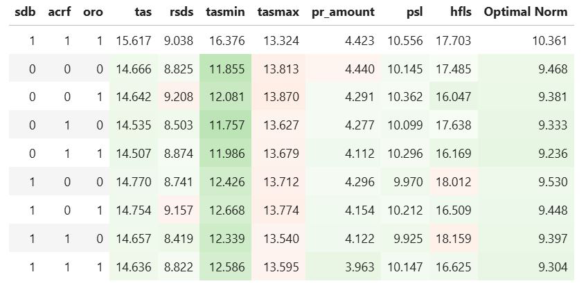
Figure 10 The variable scores (Eq. 3) for the optimal configurations with different sequences of logical switches. The first row represents the reference NWP configuration. The first three columns describe the sequence of logical switches, while the following columns give the resulting scores for the considered variables. The last column shows the optimal norm (Eq. 4). The values are color-coded with a gradient from red to green, indicating relative deficiency or improvement compared to the corresponding reference values.

From the Fig. 10 one can clearly see the positive effect of more detailed orography on the latent heat flux (hfls), as the bias is significantly reduced for all cases when oro=1. Overall, updating all external data sets (sdb, acrf, oro) = ($\mathrm{1},\mathrm{1},\mathrm{1}$) leads to the most pronounced improvements in precipitation (pr_amount) and latent heat flux over sea (hfls).

5 Discussion

The LiMMo optimization strategy demonstrates significant potential for objective calibration. While it quickly and automatically generates optimal parameter values, it requires extensive expert knowledge of the model parameters. The user must define the parameter set, ensure the sensitivity of model outputs to parameter changes, and determine the optimization objective, which is reflected in the assignment of the error norm. The computational efficiency of LiMMo allows for an extensive definition of the error norm. In this study, seven different model quantities are considered, which is a significant increase compared to previous studies. However, for simplicity, we limit the error norm to mean values (root mean square error). From a methodological perspective, it is feasible to include more sophisticated and critical quantities such as extreme precipitation (e.g., the 99th percentile of hourly precipitation over a given period), the diurnal cycle of precipitation, and/or short-wave radiation. Tuning these quantities will be a focus of future research. The current study investigates 10–15 model parameters simultaneously, a scale that was previously unfeasible. However, the linear scalability of the optimization time with respect to the number of parameters allows for a significant expansion of this range, potentially by hundreds of parameters.

Another important aspect, which is beyond the scope of this study, is the monthly weighting of the model variables in the definition of the error norm (Eqs. 3 and 4). Given the broad tuning period of six years, the computation of multi-year averages significantly reduces the imbalance of monthly internal variability (Eq. 2), ensuring that the signal-to-noise ratio is approximately equal across months. Therefore, further reduction of temporal dimensionality by considering monthly averages (Eq. 3) is sufficient to treat all months equally. However, for shorter tuning periods, the monthly imbalance in the signal-to-noise ratio may become more pronounced, especially since climate models typically exhibit greater internal variability during the summer months. In such cases, considering monthly averages could lead to an underestimation of the impact of summer months on the model quality score. A more general approach would be to introduce monthly weights for variable errors f_k,n (where k is the month index, n is the model variable index), so that the final error norm in the optimization would be

$$\mathrm{ERR}=\sum _n{c}_n\cdot \sum _k{f}_{k,n}\cdot {\displaystyle \frac{{\mathrm{RMSE}}_{k,n}}{{\mathit{\sigma }}_{k,n}}};\sum _k{f}_{k,n}=\mathrm{1}.$$

This would allow control over the contribution of monthly errors, allowing the weights f_k,n to be adjusted to balance their contribution to the overall error norm. For example, one could choose the monthly weights to be inversely proportional to the signal-to-noise ratio for the reference simulation:

$$f_{i,n}\cdot {\displaystyle \frac{{\mathrm{RMSE}}_{i,n}^{\mathrm{ref}}}{{\mathit{\sigma }}_{i,n}}}=f_{j,n}\cdot {\displaystyle \frac{{\mathrm{RMSE}}_{j,n}^{\mathrm{ref}}}{{\mathit{\sigma }}_{j,n}}},\forall i,j;\sum _k{f}_{k,n}=\mathrm{1}.$$

6 Conclusions

The current study introduces a new tool for objective tuning of regional climate models. Building on previous work (Neelin et al., 2010; Bellprat et al., 2012; Avgoustoglou et al., 2022), the LiMMo framework employs a regression-based approximation of climate model outputs. Unlike previous approaches, LiMMo primarily uses a linear regression approximation rather than a quadratic one. This choice is motivated by the cost-effectiveness of building the statistical emulator, as it requires only a linear number of dynamical simulations (at least one for each parameter). Despite its simplicity, the approximation has demonstrated high accuracy when modeling over long periods of time, as evidenced by the 6-year span considered in this study.

A second distinctive feature of LiMMo is the use of a gradient-based method to minimize the error norm relative to observations, in contrast to previously proposed Monte Carlo methods. The combination of a linear Meta-Model with fast gradient-based optimization allows the approach to scale linearly with the number of model quantities and parameters, allowing the simultaneous tuning of dozens of parameters, a task previously infeasible due to time-to-solution constraints.

The LiMMo framework was applied to the state-of-the-art regional climate model ICON-CLM, tuned to the E-OBS and HOAPS observational data sets. A total of 15 model parameters were optimized using 7 model variables that define the distance of the model to the observations. Different optimization objectives were explored by assigning different weights to the model variables in the error norm definition. In addition, optimization was performed for 8 different sequences of 3 logical switches, providing comprehensive insights to select the climate model configuration that best meets the user's priorities.

Please note that the current study is not intended to give any recommendations on the setup of ICON-CLM, but only to demonstrate the capabilities of the proposed LiMMo technique. The final decision of the model configuration should be made after careful and extensive analysis of the model quantities, and LiMMo is only one of the tools that requires expert judgment.

Appendix A: ICON parameters description

(Schulz and Vogel, 2020)

Table A1 The ICON tuning parameters for Surface Transfer Scheme (Sect. 2.4.1) and Mixing in the Planetary Boundary Layer (Sect. 2.4.2). The section number with description of parameter is given in the column “Section”. The “Parameter” column gives the name of the parameter as used in the ICON model, while the “Acronym” column shows the parameter acronym used in this article. The “Type” column indicates whether the parameter is continuous (“C”) or binary (“B”). The “Min/Ref/Max” column represent the minimum, reference, and maximum values, respectively. The “Tested values” column shows the values simulated by ICON-CLM, used for regression training. The “Description” column provides a brief explanation of each parameter.

(FAO/UNESCO, 1981)(Nachtergaele et al., 2023)(GLOBE Task Team et al., 1999)(Yamazaki et al., 2017)(Kinne, 2019)(Schaaf et al., 2021)

Table A2 The ICON tuning parameters for Cloud cover (Sect. 2.4.3) and External data sets (Sect. 2.4.4). The description of the columns is the same as in Table A1.