REtrieval Method for optical and physical Aerosol Properties in the stratosphere (REMAPv1)

Stratospheric aerosol is an important climate forcing agent as it scatters some of the incoming solar radiation back to space, thus cooling the Earth's surface and the troposphere. At the same time, it absorbs some of the upwelling terrestrial radiation that heats the stratosphere. It also plays an important role in stratospheric ozone chemistry by hosting heterogeneous reactions. Major volcanic eruptions can cause strong perturbations of stratospheric aerosol, changing its radiative and chemical effects by more than an order of magnitude. Many global climate models require prescribed stratospheric aerosol as input to properly simulate both climate effects in the presence and absence of volcanic eruptions. This paper describes REMAP, a retrieval method and code for aerosol properties that has been used in several model intercomparison projects (under the name Stratospheric Aerosol and Gas Experiment-3λ, SAGE-3λ). The code fits a single-mode lognormal size distribution for a pure aqueous sulfuric acid aerosol to aerosol extinction coefficients from observational or model data sets. From the retrieved size distribution parameters, the code calculates the effective radius; surface area density; and extinction coefficients, single-scattering albedos, and asymmetry factors of the aerosol within the wavelength bands specified for each individual climate model. We validate REMAP using balloon-borne observations after the Mount Pinatubo and Hunga Tonga–Hunga Ha`apai (HTHH) volcanic eruptions, as well as 4 decades of lidar measurements. Within the constraints of a single-mode lognormal distribution, REMAP generates realistic effective radii and surface area densities after volcanic eruptions and generally matches the lidar backscatter time series within measurement uncertainty. Deviations in aerosol backscatter by up to a factor of 2 arise when (non-volcanic) tropospheric intrusions (e.g., from wildfires) are present and the size distribution deviates significantly from the single-mode lognormal type. We describe the products that have been used in CCMI (Chemistry–Climate Model Initiative), CMIP6 (Coupled Model Intercomparison Project Phase 6 ), and other model intercomparison projects and provide practical instructions for use of the code in future applications.

1 Introduction

The stratospheric aerosol has been of scientific interest since its discovery by Christian Junge and colleagues in 1960 (Junge et al., 1961; Chagnon and Junge, 1961). Aerosol particles have an impact on the radiative balance of the Earth system (Robock, 2000; Solomon et al., 2011; Santer et al., 2014), and they host important heterogeneous chemical reactions (Hofmann and Solomon, 1989; Solomon, 1999; Tilmes et al., 2008). Therefore, global models require information on stratospheric aerosol records and climatologies.

The strength of heterogeneous chemical reactions scales with the surface area density (SAD) of stratospheric aerosols. The N₂O₅ hydrolysis on aerosol surfaces (e.g., Robinson et al., 1997) alters the partitioning of active nitrogen NO_x to total reactive nitrogen NO_y, which affects stratospheric ozone chemistry throughout the aerosol layer, especially under volcanically perturbed conditions (Fahey et al., 1993). In very cold conditions, such as in the winter polar vortex or in the vicinity of the tropical tropopause, additional heterogeneous reactions may activate chlorine from its reservoir species, leading to enhanced ozone depletion (Hanson et al., 1994; Solomon, 1999; Tilmes et al., 2008). These chlorine activating reactions occur mainly at the liquid–gas interface and, to a lesser extent, within the liquid bulk phase of these cold binary H₂SO₄-H₂O droplets. Therefore, size information is also required for the corresponding modeling of the heterogeneous reactions in addition to the SAD (Hanson et al., 1994). Besides these cold H₂SO₄-H₂O droplets, polar winter conditions also favor the formation of polar stratospheric clouds (PSCs), i.e., droplets and solid hydrate particles containing HNO₃. However, PSCs are not the subject of this article, and the transition from cold binary H₂SO₄–H₂O particles to large ternary HNO₃–H₂SO₄–H₂O droplets and hydrates must be treated individually by each global climate model.

The radiative forcing of the stratospheric aerosol has been addressed by many authors, in particular with respect to volcanic perturbations (Russell et al., 1993; Sato et al., 1993; Stenchikov et al., 1998; Robock, 2000; Stothers, 2001; Ammann et al., 2003; SPARC, 2006; Thomason et al., 2008; Vernier et al., 2011; Solomon et al., 2011; Arfeuille et al., 2013, 2014; Santer et al., 2014; Zanchettin et al., 2016). Recent major volcanic eruptions – e.g., El Chichón in 1982 and Mount Pinatubo in 1991 – led to a temporary decrease in global mean surface temperature, estimated to reach up to 0.5 K (Santer et al., 2014). The moderate volcanic eruptions since 2005 of Augustine, Soufrière Hills, Shiveluch, Kasatochi, Sarychev, and Nabro led to a moderate but persistent increase in the stratospheric aerosol (Vernier et al., 2011; Carn et al., 2017), which may partly explain the early 21st-century “warming hiatus” (Solomon et al., 2011; Santer et al., 2014; Andersson et al., 2015). Stratospheric aerosol continues to be elevated by volcanic eruptions (Ambae, Ulawun, and Raikoke) in the past few years (Carn, 2022), including the water-rich Hunga Tonga–Hunga Ha`apai (HTHH) eruption (Vömel et al., 2022), joined by other not-sulfur-dominated sources: several large wildfire events in British Columbia, Australia, and Colorado (Madhavan et al., 2022; Trickl et al., 2023). A precise description of the radiative properties of the stratospheric aerosol following such events requires an understanding of the distribution and transformation of particles, i.e., size distribution information, in the fresh volcanic plume (e.g., Sheng et al., 2015). Global size distribution data sets, however, do not exist from direct measurements and need to be retrieved from satellite measured radiative properties. Thus, their quality relies on the retrieval method. This type of data could further inform speculation as to whether artificial stratospheric SO₂ injections are a suitable candidate for partially counteracting global warming caused by greenhouse gas emissions (e.g., Crutzen, 2006; Heckendorn et al., 2009; Weisenstein et al., 2022).

The operation of global climate models requires knowledge on the radiative forcing by the stratospheric aerosol. This aerosol forcing can be either calculated online, provided that the employed model has microphysics and chemistry modules, or prescribed as external forcing, provided that a sufficiently good observational data set is available. The former requires to model the conversion of aerosol precursor gases (OCS, SO₂) via photolysis and oxidation reactions into gaseous H₂SO₄, which can condense on preexisting aerosol particles or nucleate new ones; calculate size distributions of particles and transport them throughout the stratosphere; and finally calculate by Mie theory the scattering of the incoming solar radiation and absorption of terrestrial radiation. The extensive physico-chemical modeling is computationally intensive but is now used by a number of the global climate models (Timmreck et al., 2018; Brodowsky et al., 2024). Yet, the resulting aerosol forcing may differ significantly over different models with interactive aerosols (Clyne et al., 2021; Quaglia et al., 2023), representing a major source of uncertainty. However, most global circulation models (GCMs) still rely on prescribed chemical and aerosol forcing fields, and even many chemistry–climate models (CCMs) prescribe stratospheric aerosols as a compromise between models' complexity and computational efficiency. Thus, a method of establishing the radiative forcing fields of the stratospheric aerosol for use in global climate models is required. The operation of these models typically requires the space–time-resolved data fields of aerosol extinction coefficients (AECs in text; β in mathematical notation), single-scattering albedos (SSAs; ω), and asymmetry factors (AFs; g) for each wavelength band in each of the models. Establishing these fields, together with SAD and size information, is a major prerequisite for model intercomparison projects (MIPs) (Lanzante and Free, 2008; Eyring et al., 2010; Gettelman et al., 2010; Eyring et al., 2016; Morgenstern et al., 2017).

The starting point for calculating the radiative properties of aerosols is a size distribution that characterizes an aerosol ensemble. A method to derive size distribution parameters from SAGE (Stratospheric Aerosol and Gas Experiment) II multi-wavelength aerosol extinction measurements was originally proposed by Yue (1986) and Yue et al. (1986). They used AEC ratios to solve a system of equations for the parameters of a single-mode lognormal (SLN) size distribution. More efforts to retrieve SLN size distributions followed (e.g., Stenchikov et al., 1998, and references therein; Bingen et al., 2003; Arfeuille et al., 2013; Wrana et al., 2021). In quiescent periods, the SLN size distribution approximates the stratospheric aerosol fairly well (Deshler et al., 1992; Wurl et al., 2010). However, in volcanically enhanced stratospheric aerosol, additional modes are often present (Deshler et al., 1992; Pusechel et al., 1992). Russell et al. (1996) mention that retrieved SLN size distributions can still produce accurate aerosol properties – even when the aerosol consists of two modes – given that the real distribution is not “extremely bimodal” (i.e., the modes overlap sufficiently well and do not have similar number densities). However, von Savigny and Hoffmann (2020) warn of systematic biases caused by SLN size distributions retrieved from occultation measurements. These biases apply to conditions of the stratospheric aerosol, when an SLN size distribution is insufficient to capture the real distribution. While Thomason et al. (2008) retrieved aerosol SAD for two monodisperse modes with prescribed number densities, most observational products do not provide enough independent information (wavelength channels) to reasonably constrain all parameters of a dual-mode lognormal (DLN) size distribution. This was shown for SAGE data by Knepp et al. (2024). In this paper, we focus on a generalized best-fit retrieval approach for SLN size distributions and discuss the limitations of the SLN approximation using comparisons with balloon-borne in situ and lidar measurements.

Dedicated satellite missions to observe the stratospheric aerosol began in 1979 with the SAGE program. Spanning 2 full decades (1984–2005), the SAGE II data are a cornerstone of stratospheric aerosol observations, which has been used extensively. It includes AECs at wavelengths of 1020, 525, 452, and 386 nm, providing information on the size of aerosol particles. However, caution is advised as the uncertainties in these four channels differ considerably, with systematically higher zonal standard deviations in channels at 452 and 386 nm. The latest release of SAGE II data is version 7 (Damadeo et al., 2013), with improved retrieval algorithms compared to earlier versions. In June 2017 the operational period of the Stratospheric Aerosol and Gas Experiment III mounted externally on the International Space Station (SAGE III/ISS; hereafter called SAGE III since we do not discuss SAGE III on the Meteor-3M satellite (SAGE III/M3M) in this article) started providing the SAGE III aerosol extinction on nine different wavelengths, continuing the record of the SAGE instrument family after an interruption of over a decade. In addition to the improved range of the wavelength range further into the near-infrared range (the longest wavelength of SAGE III is 1544 nm as compared to its predecessor SAGE II with 1020 µm), a cloud-cleared version of the SAGE III data has been introduced. The establishment of an official aerosol/cloud categorization algorithm (Kovilakam et al., 2023) eliminates a time-intensive step in pre-processing that previously had to be done in one of various different ways by the user. The Global Space-based Stratospheric Aerosol Climatology (GloSSAC) incorporates both the SAGE II and SAGE III data sets as well as CLAES-ISAMS (Cryogenic Limb Array Etalon Spectrometer – Improved Stratospheric and Mesospheric Sounder, Lambert et al., 1997), HALOE (Halogen Occultation Experiment, Hervig et al., 1995), OSIRIS, and CALIOP data (described in Sect. S1.3 in the Supplement) to produce a continuous AEC product from 1979 onward (see the Supplement for more information on data sets). Since 2012, the Ozone Mapping and Profiler Suite Limb Profiler (OMPS-LP) on board the Suomi NPP satellite has provided limb scatter measurements. From these data, Taha et al. (2021) have retrieved AECs on six wavelengths; however, they report limited accuracy in some of the channels. In the future, the OMPS-LP data might be incorporated into GloSSAC as well, potentially making the composite more robust. Furthermore, the new Climate Data Record of Stratospheric Aerosols (CREST) was published recently (Sofieva et al., 2024), providing a single-wavelength composite of six limb scatter and occultation measurement data sets.

In this paper, we describe and validate the latest version of a generalized method to retrieve SLN size distributions for sulfuric aerosol from the abovementioned AEC data sets and use these to calculate a variety of aerosol optical and mass-related properties. The method is termed REtrieval Method for Aerosol Properties (REMAP). Its strength lies in its flexibility to provide optical properties for any prescribed wavelength band so the output can be tailored to the spectral resolution of any radiation scheme. The REMAP method, previously termed SAGE-4λ and SAGE-3λ, has been used in multiple past and ongoing MIPs (Table 1) but has not yet been described in sufficient detail. Arfeuille et al. (2013) described the preparation of a Mount Pinatubo forcing data set using this method. However, only a brief description of this specific use case was provided. Here, we first give an overview of all projects, in which REMAP was used including the resulting data sets. We then describe the general methodology in full and give practical information on how to use the code followed by a product validation against measurements.

Table 1 Data sets produced with REMAP and used in different model intercomparison projects to prescribe a uniform stratospheric aerosol.

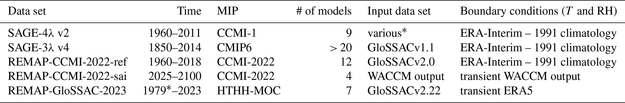
^∗ Even though the data set was established for the entire duration of the GloSSACv2.22 data set (1979–2023), this MIP only required forcing from 2019–2023.

2 Product overview

The predecessors of REMAP were first used to create the aerosol forcing for global models within the IGAC/APARC Chemistry–Climate Model Initiative (CCMI) Phase 1 experiment (Eyring et al., 2013). To this end, different satellite data sets were selected, screened for cloud contamination, interpolated, and ultimately combined to create a continuous and consistent 50-year record (1960–2011). This record was termed SAGE-4λ because its backbone was the four SAGE II wavelengths (4λ). In addition to SAGE II data, some other satellite AECs, sun photometer data, and information from tropical ground-based lidars for the filling of data gaps under volcanically opaque conditions were combined. For details about the SAGE-4λ record, including gap filling, see Sect. S1. In preparation for Coupled Model Intercomparison Project Phase 6 (CMIP6), Thomason et al. (2018) constructed the first version of GloSSAC (v1.0), which contained an error in the conversion of CLAES data to SAGE II wavelengths. This was corrected in v1.1 as described by Kovilakam et al. (2020), whereupon we corrected the SAGE-4λ record and made it available to the modeling groups involved in CMIP6 for aerosol forcings. We based this data set on the homogenized single product GloSSAC rather than incorporating different sources as in CCMI-1. Although the CMIP6 forcing data set is primarily based on SAGE II, we no longer used the shortest SAGE II wavelength at 386 nm since its quality was insufficient to improve the result. The data set was therefore designated as SAGE-3λ. Revell et al. (2017) describe the CLAES/SAGE II conversion error in their corrigendum and show differences in the aerosol loading and forced temperature and ozone anomalies that arise from using the improved SAGE-3λ data set versus the previous SAGE-4λ. Shortly after we released SAGE-3λ to the modeling community, GloSSAC was further updated with new and improved satellite data sets as GloSSACv2.0, described by Kovilakam et al. (2020). It also extended to the end of 2018 and was subsequently used for the historical hindcast period of the CCMI Phase 2 (CCMI-2022) modeling activity (Plummer et al., 2021), which required prescribed radiative forcing data sets for stratospheric aerosol. Another set of sensitivity runs within CCMI-2022 simulated a climate intervention scenario and was called senD2-sai. For this experiment, the forcing needed to be derived from a separate model simulation – instead of observations – and spectrally regridded for participating models. Details on this procedure are given in Sect. 3.5. Finally, the version of GloSSAC at the time of writing this article (v2.22) includes an aerosol/cloud categorization algorithm (Kovilakam et al., 2023) and extends to the end of 2023. Finally, we used all available GloSSAC wavelengths with their associated zonal standard deviations (eliminating the quality reduction caused by the shortest SAGE wavelength) for the Hunga Tonga–Hunga Ha`apai Impact Model Observations Comparison (HTHH-MOC) forcings (Zhu et al., 2024).

Table 1 shows all data sets produced with REMAP that were distributed to modeling groups along with information about the respective inputs. In summary, REMAP was used to provide data of stratospheric aerosol optical properties to

• 9 models participating in CCMI-1 in support of ozone and climate assessments (Eyring et al., 2013; Hegglin et al., 2014) (SAGE-4λv2 data set, Luo, 2013);

• some 20 models participating in the Coupled Model Intercomparison Project Phase 6 (CMIP6) to better understand past, present, and future climate in a multi-model context (Eyring et al., 2016) (SAGE-3λv4 data set, Luo, 2017);

• 12 models participating in the CCMI Phase 2/CCMI-2022 historical runs (also following CMIP6 forcing guidelines) (Plummer et al., 2021) (REMAP-CCMI-2022-ref data set, Luo, 2020);

• 4 models participating in the CCMI-2022 senD2-sai experiment to assess a climate intervention (CI) scenario (Plummer et al., 2021) (REMAP-CCMI-2022-sai data set, Jörimann, 2023; more information in Sect. 3.5);

• 7 models participating in the Hunga Tonga–Hunga Ha`apai Impact Model Observations Comparison (HTHH-MOC) to examine the effects of the largest phreatomagmatic explosion in the satellite record (Zhu et al., 2024) and to a single-model study examining effects of the HTHH eruption (Kuchar et al., 2025) (REMAP-GloSSAC-2023 data set, Jörimann, 2024).

3 Description of the REtrieval Method for Aerosol Properties (REMAP)

In order to estimate the radiative properties of the aerosol particles, the size distribution is required. It can be retrieved, in a best-fit sense, by comparing the calculated AECs of all size distributions in the allowed parameter space against observations. With the size distribution characterized, the AEC, SSA, and AF of the aerosol ensemble can be calculated using Mie theory (Bohren and Huffman, 1998). To this end, we assume that the stratospheric aerosol comprises pure aqueous sulfuric acid solution droplets. The sulfuric acid concentration is calculated from the atmospheric relative humidity and temperature using the water vapor pressure of aqueous sulfuric acid (Luo et al., 1995; Carslaw et al., 1995). For the relative humidity (RH) and temperature, both model output and reanalysis data can be used. The refractive index as a function of temperature and H₂SO₄ concentration is then calculated using the parameterization of Luo et al. (1996) for visible wavelengths and measurements of Biermann et al. (2000) for infrared wavelengths. In this way, we take the concentration and temperature dependence of the refractive index into account in both the size distribution retrieval procedure and the final calculation of the optical properties.

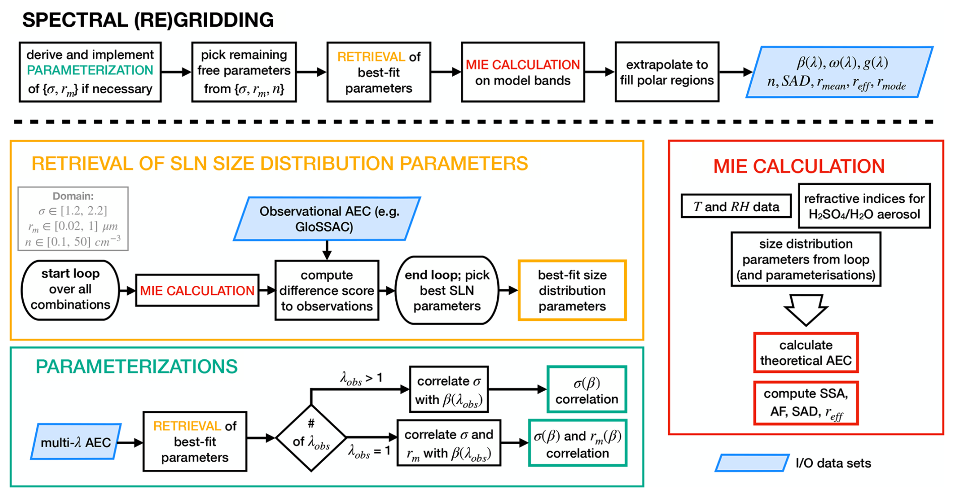
Figure 1 Scheme of the REMAP algorithms in general form. The spectral regridding method always involves the retrieval (yellow box) of aerosol size distribution parameters (n, r_m, σ) from observational AEC data and the Mie calculation (red box) of radiative properties (aerosol extinction coefficient AEC(λ), single-scattering albedo SSA(λ), asymmetry factor AF(λ)) in spectral resolution of choice. Optionally, the retrieval procedure is improved and in some cases made possible in the first place by parameterizations (turquoise box) separately retrieved from a data set with a high enough number of channels (multi-λ data set). For details see text.

3.1 Retrieval of the size distribution

Figure 1 summarizes REMAP in its most general form and latest state. The core element is the retrieval procedure (yellow box), which uses the Mie calculation (red box) and is itself used in the optional derivation of parameterizations (turquoise box). The retrieval procedure operates on a data set of AECs from either the measurements or the output of a model simulation, which here we call the observational AEC data set.

The basic assumption throughout the whole method is that the aerosol size distribution of the aerosols can be represented by a SLN particle size distribution:

$$\begin{array}{}\text{(1)}& {\displaystyle \frac{\mathrm{d}n\left(r\right)}{\mathrm{d}r}}=n{\displaystyle \frac{\mathrm{1}}{\sqrt{\mathrm{2}\mathit{\pi }}r\ln \mathit{\sigma }}}\exp \left(-{\displaystyle \frac{{\ln }^{\mathrm{2}}(r/r_{\mathrm{m}})}{\mathrm{2}{\ln }^{\mathrm{2}}\mathit{\sigma }}}\right).\end{array}$$

There are three unknowns: the number density, n; the median radius, r_m; and the geometric standard deviation σ of the aerosol SLN size distribution. Ideally, the retrieval procedure fits all three parameters to the observational AECs. In that case, the parameters can be directly retrieved by picking the parameter combination that best reproduces the measured AECs. However, this requires data on at least three wavelengths of good quality (see Sect. 3.2 for what constitutes good quality). If there is no complete coverage with at least three wavelengths of good quality or to simply improve the output consistency (cf. Arfeuille et al., 2013), parameterizations can be used to replace one or two parameters. Here, we describe the method systematically for the distinct cases of ≥ 3, 2, and 1 available wavelength.

• a.

  Three or more wavelengths: the three parameters n, r_m, and σ, which fit best to the measured AECs, are directly retrieved (full retrieval, yellow box in Fig. 1). The best-fit parameters are selected based on the minimum difference score D between measured and theoretical AECs across the range of possible parameter values. To achieve this, a program goes through the following steps for each set of parameters in the domain (grey box):

  • The theoretical AEC k_theor are calculated on the same wavelengths λ that are available in the observational data using Mie theory (red box).

  • For each wavelength the difference score D of the calculated to the measured extinction coefficients k_obs is computed.

  • If available, the zonal standard deviation ς of the measurements is also taken into account. The theoretical-to-observed AEC ratio for each wavelength is weighted inversely with the associated scatter (i.e., the zonal standard deviation), which is typically higher at smaller wavelengths due to the higher molecular-to-aerosol extinction ratio. If no zonal standard deviations are available, each wavelength is weighted the same.

  • The ratios for each wavelength are summed up to a total (weighted) difference score. The program keeps track of the lowest achieved difference score and the corresponding parameters n, r_m, and σ. It only updates the parameters once a lower difference score is generated. After all combinations are run, the best fit (according to Mie theory and assuming a SLN size distribution) is found.

  • Summarized in mathematical notation, the difference score

    $$\begin{array}{}\text{(2)}& \begin{array}{rl}& D=\sum _{i=\mathrm{1}}^n{\left[\ln \left({\displaystyle \frac{{\mathit{\beta }}_{\text{theor}}\left({\mathit{\lambda }}_i\right)}{{\mathit{\beta }}_{\text{obs}}\left({\mathit{\lambda }}_i\right)}}\right)\cdot \text{weight}\right]}^{\mathrm{2}},\\ & \text{weight}={\displaystyle \frac{\frac{{\mathit{\beta }}_{\text{obs}}\left({\mathit{\lambda }}_i\right)}{\mathit{\varsigma }\left({\mathit{\lambda }}_i\right)}}{\sqrt{{\sum }_{j=\mathrm{1}}^n{\left(\frac{{\mathit{\beta }}_{\text{obs}}\left({\mathit{\lambda }}_j\right)}{\mathit{\varsigma }({\mathit{\lambda }}_j}\right)}^{\mathrm{2}}}}},\end{array}\end{array}$$

    is minimized at each grid point. From this difference score, we also report an error (E) given by

    $$\begin{array}{}\text{(3)}& E=\sqrt{D}.\end{array}$$

    The error (E) typically decreases with increasing altitude. This is illustrated in Fig. 2, which is a latitude-altitude map of the mean error over 5 years that came from a retrieval on six wavelengths of SAGE III data. The trend comes from a general decrease in the zonal standard deviation ς with increasing height, probably due to shorter path lengths and less saturation of the occultation measurements at greater heights. Above 27 km, the error steps to higher values again; this is due to those data coming from a high-altitude climatology instead of (mostly) transient satellite data. In the lowest stratospheric region just above, the tropopause ς sometimes spikes locally, which is reflected in Fig. 2. Also, tropospheric intrusions could cause a strongly multi-modal aerosol size distribution there. The actual error values depend on the number of wavelengths, the availability of measurement zonal standard deviation, and the strength of the AEC signal itself. Therefore, it cannot be used to compare the retrieval quality between retrievals, where any of these factors vary, only within a single run.

  To improve the convergence of the algorithm, we constrained the range of σ to 1.2–2.2, the range of r_m to 0.02–1 µm, and the range of n to 0.1–50 cm⁻³. These upper and lower limits are physically reasonable constraints derived from the long-term in situ measurements over Laramie, Wyoming (Deshler, 2008). For the Mie calculation, the size distribution and aerosol refractive indices are required. The refractive index of a medium depends on its chemical composition, and to determine this, the environmental variables temperature and RH are also required to calculate the real and imaginary parts of the aerosol refractive indices (Luo et al., 1996; Biermann et al., 2000). Table 1 shows where these boundary conditions came from for different REMAP data sets. The results of a full retrieval can still be heterogeneous when all three parameters are unconstrained within the permitted parameter space. To improve this, a parameterization (see the turquoise box in Fig. 1) lays a further constraint on the retrieval process. With the parameterization function of the form σ(k_param) the retrieval algorithm can be repeated, but this time only fitting the remaining two parameters.

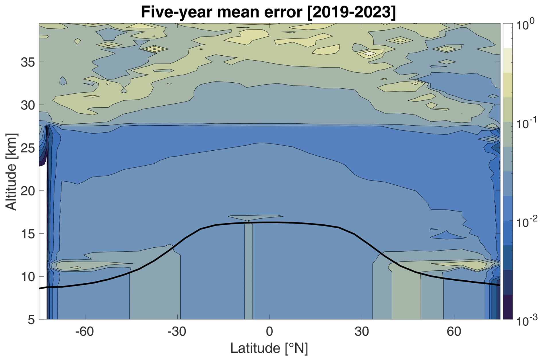
Figure 2 Latitude–altitude plot of the 5-year mean error from a retrieval of six SAGE III wavelengths where available and gaps filled with GloSSACv2.22. The black line indicates the average tropopause height. The Junge layer is discernible from the minimum error values. The distinct rise in error above 27 km at all latitudes comes from the observational data set GloSSACv2.22 itself, which includes a high-altitude climatology.

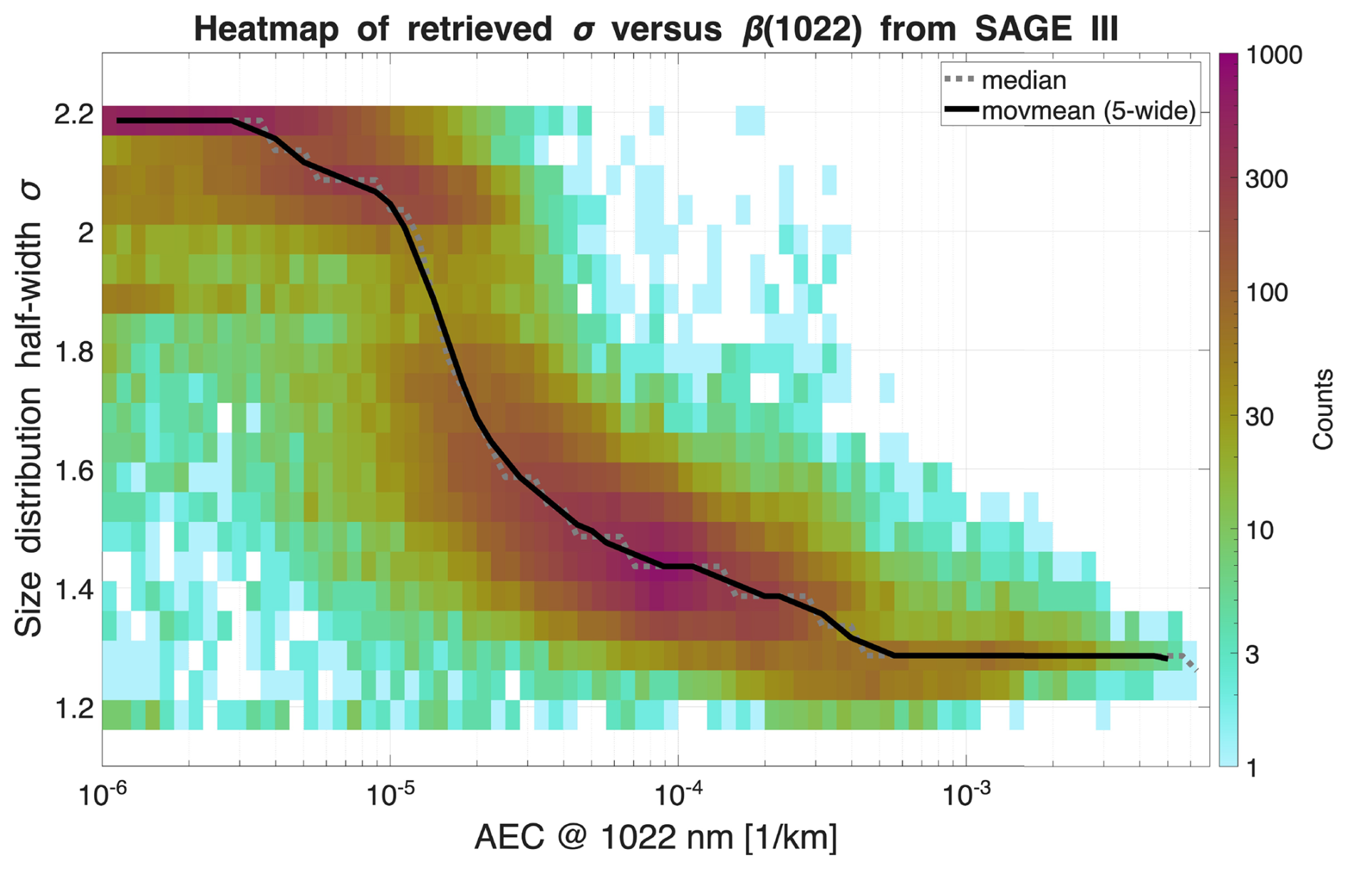
Figure 3 2D histogram of all σ values retrieved from data of six selected SAGE III wavelengths (June 2017–December 2023, above 20 km) against their corresponding aerosol extinction coefficients. The dotted grey line shows the median value for every extinction coefficient bin; the solid black line shows the moving mean of the median at a width of five bins. A function can be fitted to the black line to get the parameterization function σ(β₁₀₂₂).

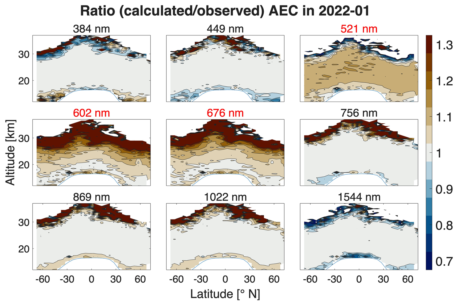
Figure 4 Ratios of the calculated to measured monthly mean AECs from SAGE III for January 2022. The calculated AECs are based on a retrieval with six good-quality SAGE III wavelengths (black font), with three wavelengths (521, 602, and 676 nm; red font) removed due to systematic biases. From this retrieval of selected wavelengths, theoretical AECs are again calculated on all nine original wavelengths to demonstrate the biases.

• b.

  Two wavelengths: if only two different wavelengths are available for the retrieval, a full retrieval cannot be performed, and a parameterization function is required to start the process. These functions make use of an empirical relationship of one size distribution parameter with the observational AEC data, thus eliminating 1 degree of freedom. To establish the empirical relationship, another data set is required that is apt for a full retrieval. We found that the distribution geometric standard deviation σ and median radius r_m are best suited for parameterizations since they most reliably produce monotonic parameterization functions. Figure 3 shows a 2D histogram of the SAGE III extinction coefficients at 1022 nm and the retrieved σ above 20 km. We used AECs on the wavelength of 1022 nm because they were very well reproduced by the algorithm (cf. Fig. 4). An eighth-grade Fourier fit to the median (red line in Fig. 3 was used to parameterize σ in this case:

  $$\begin{array}{}\text{(4)}& \begin{array}{rl}& \mathit{\sigma }=\\ & \left\{\begin{array}{ll}\mathrm{2.19}& \text{if }\ln {\mathit{\beta }}_{\mathrm{1022}}<-\mathrm{13},\\ \mathrm{1.636}& \\ \begin{array}{rl}& -\mathrm{0.09632}\cos (\ln {\mathit{\beta }}_{\mathrm{1022}}\cdot \mathrm{0.6463})\\ & -\mathrm{0.4427}\sin (\ln {\mathit{\beta }}_{\mathrm{1022}}\cdot \mathrm{0.6463})\\ & -\mathrm{0.08697}\cos (\mathrm{2}\ln {\mathit{\beta }}_{\mathrm{1022}}\cdot \mathrm{0.6463})\\ & +\mathrm{0.1495}\sin (\mathrm{2}\ln {\mathit{\beta }}_{\mathrm{1022}}\cdot \mathrm{0.6463})\\ & +\mathrm{0.01438}\cos (\mathrm{3}\ln {\mathit{\beta }}_{\mathrm{1022}}\cdot \mathrm{0.6463})\\ & -\mathrm{0.03937}\sin (\mathrm{3}\ln {\mathit{\beta }}_{\mathrm{1022}}\cdot \mathrm{0.6463})\\ & -\mathrm{0.02212}\cos (\mathrm{4}\ln {\mathit{\beta }}_{\mathrm{1022}}\cdot \mathrm{0.6463})\\ & +\mathrm{0.06559}\sin (\mathrm{4}\ln {\mathit{\beta }}_{\mathrm{1022}}\cdot \mathrm{0.6463})\\ & +\mathrm{0.0277}\cos (\mathrm{5}\ln {\mathit{\beta }}_{\mathrm{1022}}\cdot \mathrm{0.6463})\\ & -\mathrm{0.02724}\sin (\mathrm{5}\ln {\mathit{\beta }}_{\mathrm{1022}}\cdot \mathrm{0.6463})\\ & -\mathrm{0.005375}\cos (\mathrm{6}\ln {\mathit{\beta }}_{\mathrm{1022}}\cdot \mathrm{0.6463})\\ & +\mathrm{0.009788}\sin (\mathrm{6}\ln {\mathit{\beta }}_{\mathrm{1022}}\cdot \mathrm{0.6463})\\ & +\mathrm{0.01021}\cos (\mathrm{7}\ln {\mathit{\beta }}_{\mathrm{1022}}\cdot \mathrm{0.6463})\\ & -\mathrm{0.01863}\sin (\mathrm{7}\ln {\mathit{\beta }}_{\mathrm{1022}}\cdot \mathrm{0.6463})\\ & -\mathrm{0.01368}\cos (\mathrm{8}\ln {\mathit{\beta }}_{\mathrm{1022}}\cdot \mathrm{0.6463})\\ & +\mathrm{0.004736}\sin (\mathrm{8}\ln {\mathit{\beta }}_{\mathrm{1022}}\cdot \mathrm{0.6463})\end{array}& \begin{array}{r}\text{if }-\mathrm{13}\le \ln {\mathit{\beta }}_{\mathrm{1022}}\\ \le -\mathrm{7.5},\end{array}\\ \mathrm{1.28}& \text{if }\ln {\mathit{\beta }}_{\mathrm{1022}}>-\mathrm{7.5}.\end{array}\right.\end{array}\end{array}$$

  We summarize different existing parameterization functions for different past time periods in the Supplement. (All except the last parameterization therein were used to make the SAGE-4λ record.) The last table entry there is the parameterization given above, which was derived from SAGE III data and used for the HTHH-MOC activity. Because SAGE III has the highest number of useful channels across a broad spectral range out of all satellite data sets, we further recommend this parameterization for general use, i.e., for time periods not covered by observations, outside of 1979–2023.

  One example of the two-wavelength case is the forcing for the HTHH-MOC activity. The observational data set used for this retrieval was GloSSAC version 2.22, which provides full coverage on two wavelengths (525 and 1020 nm). With GloSSAC being short one channel to allow for a full retrieval, one free parameter needed to be eliminated. SAGE III data available between June 2017 and December 2023 provided six wavelengths of good quality (out of the nine total) over the time period of interest and was therefore used as the multi-λ data set (see the turquoise box in Fig. 1 to get the empirical relationship between measured AECs and σ).

• c.

  Periods with only single-wavelength aerosol extinction measurements: under these conditions, an additional parameterization of r_m or σ (whichever has not yet been parameterized) as a function of a good-quality wavelength replaces yet another free parameter, leaving the aerosol number density n as the only remaining unknown, which is retrieved using the only measured AEC k_obs. The algorithm finds the value for n that minimizes D. This comes with potentially large, inter-dependent uncertainties for both r_m and σ and is thus likely to produce inaccurate results. For the historic SAGE-3λ record, more sophisticated methods were used in this case, which are documented in Sect. S1.

3.2 Wavelength quality

Assessing the quality of each available wavelength is vital for a consistent and useful size distribution retrieval. The number of good-quality wavelengths available determines the protocol for REMAP as described in the previous section. Satellite measurements rely on some algorithm to retrieve AEC data. Such an algorithm may already make assumptions about the aerosol size distribution. Notably, to retrieve AECs for limb scatter measurements, some aerosol size distribution is assumed beforehand. This is necessary to produce such data in the first place; however, the procedure must be checked before using satellite data for REMAP. If there are strong constraints on the product or biases or low accuracy are reported for any channels of a satellite product, care must be exercised when selecting REMAP input data. In composite products that synthesize different data sets, measurements are already processed and may have been transposed onto new wavelengths. If this is the case or if a number of wavelengths have been made into a greater number of wavelengths, the method used must be checked as the information content in each channel may be limited. Ideally, each channel should represent a separate physical measurement.

Selecting a good-quality wavelength was essential for the SAGE III parameterization (Eq. 4). In this case, using all nine wavelength channels leads to an ambiguous (non-monotonic) parameterization (see Fig. S5). Only after assessing each wavelength and various wavelength combinations did we achieve the correlation in Fig. 3. This principle is further illustrated in Fig. 4, which shows the ratio of calculated divided by observed AECs from 1 month of SAGE III. The size distribution retrieval was performed on a selection of six (black font) out of the nine available wavelengths. From this the theoretical AECs were again calculated on all measurement wavelengths so as to compare the result on all channels. The three wavelengths that were omitted in the retrieval show significantly biased ratios, while the other six achieve agreement within ± 2.5 % in the Junge layer region. The biases are expected since the measurements on the biased channels did not contribute to the constriction of the size distribution parameters. However, the ratios in the other channels diverge significantly from 1 if the retrieval is performed on all nine wavelengths. Thus, the retrieval was improved by omission of biased channels. To identify biased channels, ratios could be calculated for many different combinations of retrieval wavelengths and then compared, but this is a lengthy process. In the next two sections, we describe two analytic parameters that help evaluate the wavelength quality of each channel of an observational data set.

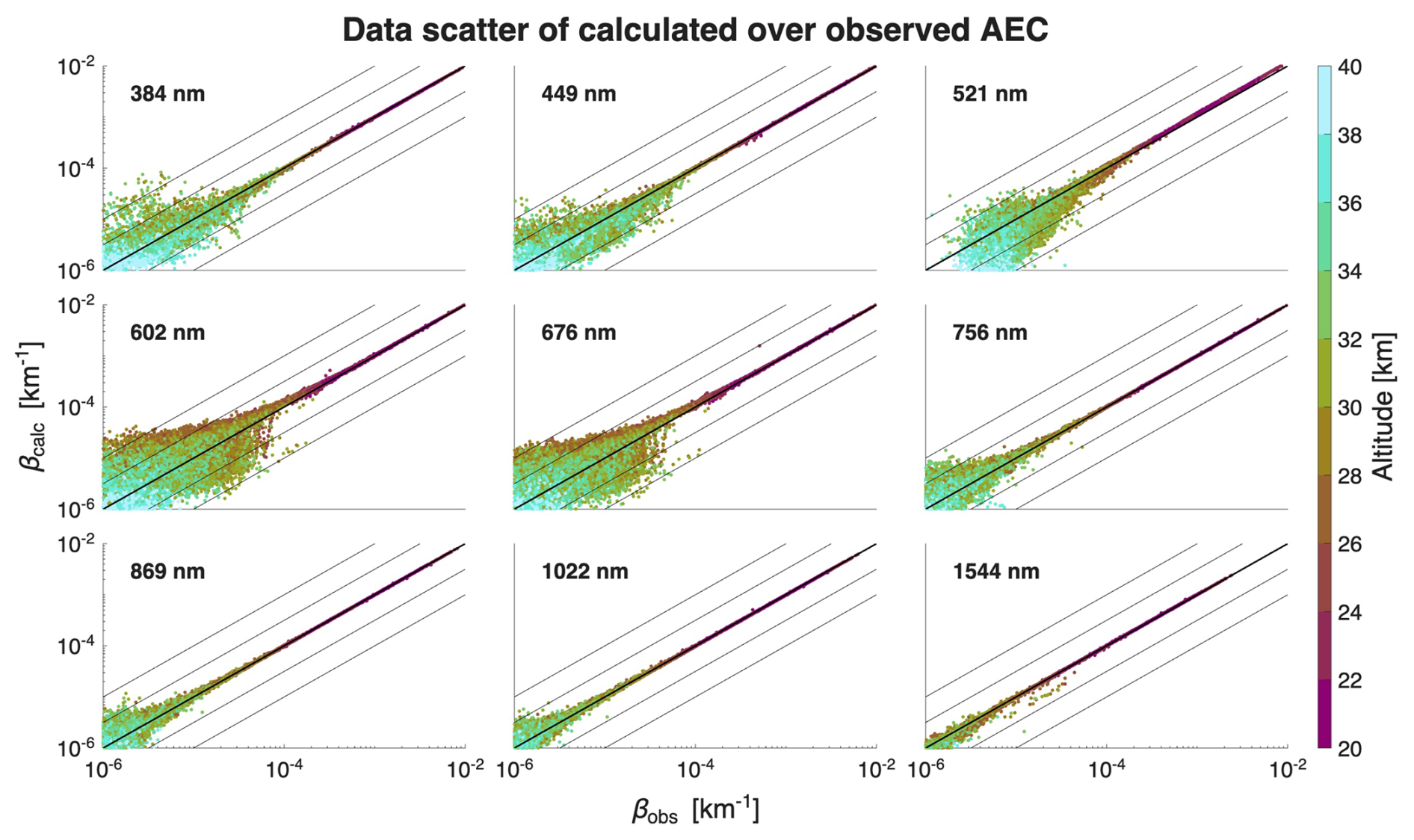
Figure 5 Scatter plots correlating calculated and measured AEC β on the nine SAGE III channels for all measurements above 20 km. To calculate the AECs from Mie theory, the SLN size distribution was retrieved by fitting its parameters to all nine wavelengths simultaneously. The calculated AECs were then computed on all same nine wavelengths again. Symmetric scatter around the thick black line indicates a poorer signal-to-noise ratio, while the center of the point cloud veering off the line indicates a bias on the affected wavelength. The colors are coded to the height of the measurement, with smaller AECs typically coming from greater heights.

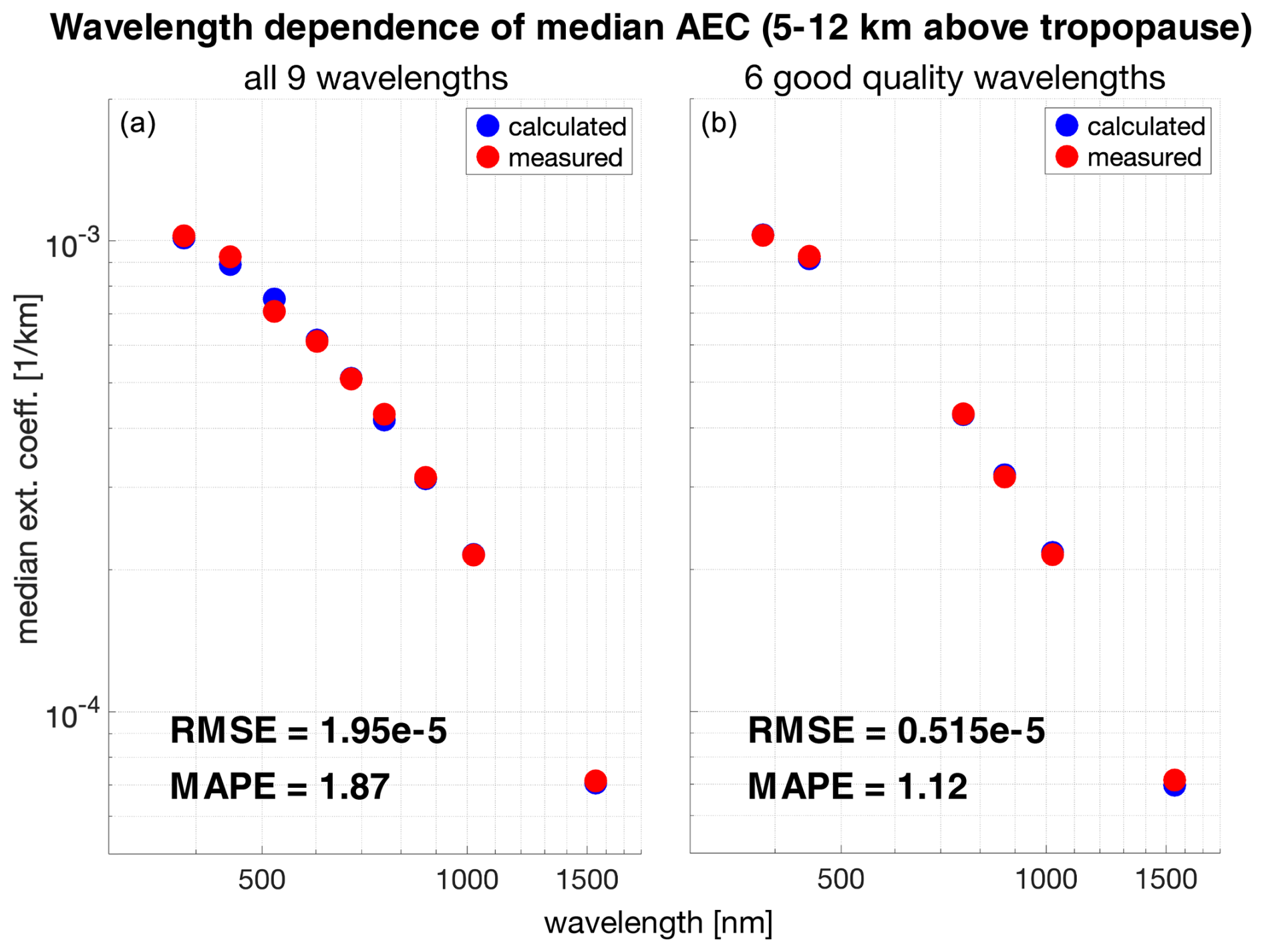
Figure 6 Color index plot of the calculated and measured SAGE III median aerosol extinction coefficients between 5 and 12 km above the mean tropopause, illustrating their wavelength dependence. The calculated aerosol extinction coefficients on the left (a) are based on a size distribution retrieval using all nine SAGE III wavelengths, whereas a selection of six good-quality wavelengths is made for the retrieval for the plot on the right (b). The blue points are governed by Mie theory and trace out an ideal wavelength dependence while also trying to fit the observations as well as possible. The residual mean square errors (RMSEs) and mean absolute percentage errors (MAPEs) both decrease with a retrieval based on selected good quality wavelengths, improving the fit.

3.2.1 Data scatter

Shorter wavelengths tend to be more scattered due to the higher molecule-to-aerosol extinction ratio. (Because of this sensitivity, shorter wavelengths are also more susceptible to uncertainties in pressure and temperature.) This effect becomes most pronounced for AEC < 10⁻⁴ and is visible in Fig. 5. However, for longer wavelengths as well, the instrument design and sensitivity can produce systematic data scatter fingerprints. This is exemplified in SAGE III/ISS, which is mounted on the international space station, a unique platform with distinct challenges. Leckey et al. (2021) describe these in detail alongside the advantages. A key feature that degraded the signal-to-noise ratio for more than half of the occultation events is an optical window designed to avoid contamination of the instrument as rockets approach the ISS. In comparison, SAGE II was flown on a smaller, unserviced spacecraft that was not exposed to exhaust gases from docking maneuvers. Data scatter is somewhat corrected for in data sets that include (zonal) standard deviations (e.g., GloSSAC), where the algorithm can then assign less weight to data points with a higher standard deviation. Based on Fig. 5, we rejected the wavelengths of 602 and 676 nm because the ratios scatter strongly off the 1:1 line even for altitudes below 30 km. The wavelength of 521 nm also shows significant bias toward underestimated calculated AECs already at low altitudes. This is consistent with Fig. 4, where the 521 nm panel clearly shows a low bias around 5 % for the calculated $/$ observed ratio.

3.2.2 Color index

The theoretical AECs given by Mie theory have a wavelength dependence. This dependence can be seen in the log-log color index plots in Fig. 6. The blue and red points are the median calculated and measured SAGE III AECs between 7 and 12 km above the mean tropopause. Two full retrievals are shown, one with all nine SAGE III wavelengths and one with exclusion of the three wavelengths in red font in Fig. 4. Since the blue points follow from Mie theory, they represent an idealized AEC function of wavelength. The measured red points do not perfectly trace out such an idealized dependence if there are biases in any of the wavelengths. This is evident in the left panel. Because REMAP finds the size distribution parameters that best fit the observations, it is not always clear from these color index plots which wavelengths are biased. However, this analysis definitively shows that the chosen ensemble of six wavelengths in the right plot yields theoretical AECs that are in better agreement with the measured AECs, reducing the root mean square error (RMSE) to a fourth and the mean absolute percentage error by 0.75 %.

3.3 Calculation of aerosol properties

In this next step, we calculate the AEC, SSA, and AF for the wavelength bands of individual global models using Mie theory. The extinction coefficient β of an aerosol ensemble at a given wavelength λ is given by

$$\begin{array}{}\text{(5)}& \mathit{\beta }\left(\mathit{\lambda }\right)=\int {\displaystyle \frac{\mathrm{d}n\left(r\right)}{\mathrm{d}r}}{C}_{\text{ext}}(\mathit{\lambda },r)\mathrm{d}r,\end{array}$$

where C_ext(λ,r) is the extinction cross section of a spherical droplet with radius r, which is readily calculated by Mie theory (Bohren and Huffman, 1998). The calculation of C_ext(λ,r) requires the real and imaginary parts of the refractive index as a function of RH and temperature. We obtain the refractive indices from Luo et al. (1996) for wavelengths between 0.35 and 2 µm. For λ < 0.35 µm, we simply use the refractive index at 0.35 µm. We consider the imaginary part of the refractive index for λ < 2 µm to be zero, i.e., negligible absorption. This assumption is well justified because the absorption in the wavelength range of 0.2–2 µm of aqueous sulfuric acid solution is indeed very small (Jonasz and Fournier, 2007). For λ < 0.2 µm, there are some strong absorption features for aqueous H₂SO₄–H₂O solutions; however, the power in the solar radiation for λ < 0.2 µm is negligible compared to the total solar radiation. For wavelengths longer than 2 µm, we use the values reported in Biermann et al. (2000), which extend both the real and imaginary part up to 20 µm. Beyond that point, the refractive indices remain constant at the last reported value. In Eq. (5), the term $\mathrm{d}n/\mathrm{d}r$ characterizes the SLN size distribution (Eq. 1) that the extinction cross section is multiplied by along the radius dimension and then integrated.

As the global models operate with wavelength bands, we need to perform a weighting of β(λ) over a wavelength region assuming Planck's law for a black body:

$$\begin{array}{}\text{(6)}& B(\mathit{\lambda },T_{\mathrm{b}})={\displaystyle \frac{\mathrm{2}h{c}^{\mathrm{2}}}{{\mathit{\lambda }}^{\mathrm{5}}}}{\displaystyle \frac{\mathrm{1}}{\text{exp}\left(\frac{hc}{\mathit{\lambda }{k}_{\mathrm{B}}{T}_{\mathrm{b}}}\right)-\mathrm{1}}}.\end{array}$$

Here, B is the radiation intensity, h is the Planck constant, c is the speed of light, k_B is the Boltzmann constant, and T_b is the temperature of the black body. A black body temperature of 5900 K is used for the solar bands and 255 K for the terrestrial bands (representing the radiative temperature of planet Earth). The weighted extinction coefficient $\stackrel{\mathrm{‾}}{\mathit{\beta }}$ for the band from wavelength λ₁ to λ₂ is calculated as

$$\begin{array}{}\text{(7)}& \stackrel{\mathrm{‾}}{\mathit{\beta }}({\mathit{\lambda }}_{\mathrm{1}},{\mathit{\lambda }}_{\mathrm{2}})={\displaystyle \frac{{\int }_{{\mathit{\lambda }}_{\mathrm{1}}}^{{\mathit{\lambda }}_{\mathrm{2}}}B(\mathit{\lambda },T_{\mathrm{b}})\mathit{\beta }\left(\mathit{\lambda }\right)\mathrm{d}\mathit{\lambda }}{{\int }_{{\mathit{\lambda }}_{\mathrm{1}}}^{{\mathit{\lambda }}_{\mathrm{2}}}B(\mathit{\lambda },T_{\mathrm{b}})\mathrm{d}\mathit{\lambda }}}.\end{array}$$

The single-scattering albedo ω is the ratio of weighted scattering coefficient $\stackrel{\mathrm{‾}}{\mathit{\delta }}$ to the weighted extinction coefficient

$$\begin{array}{}\text{(8)}& \mathit{\omega }={\displaystyle \frac{\stackrel{\mathrm{‾}}{\mathit{\delta }}}{\stackrel{\mathrm{‾}}{\mathit{\beta }}}},\end{array}$$

where $\stackrel{\mathrm{‾}}{\mathit{\delta }}({\mathit{\lambda }}_{\mathrm{1}},{\mathit{\lambda }}_{\mathrm{2}})$ for the band bounded by λ₁ to λ₂ is calculated analogously to $\stackrel{\mathrm{‾}}{\mathit{\beta }}$ from Eqs. (5)–(7).

The asymmetry factor g for a given wavelength λ of a droplet of radius r is defined as (Bohren and Huffman, 1998)

$$\begin{array}{}\text{(9)}& g(\mathit{\lambda },r)={\displaystyle \frac{{\int }_{\mathrm{\Omega }}\frac{\mathrm{d}{C}_{\text{sca}}(\mathit{\lambda },r,\mathit{\theta })}{\mathrm{d}\mathrm{\Omega }}\text{cos}\left(\mathit{\theta }\right)\text{d}\mathrm{\Omega }}{C_{\text{sca}}(\mathit{\lambda },r)}},\end{array}$$

with a scattering cross section C_sca(λ,r) and a differential scattering cross section $\mathrm{d}{C}_{\text{sca}}/\mathrm{d}\mathrm{\Omega }$. The asymmetry factor for a given wavelength band g(λ₁,λ₂) is given by integrating over the size of particles and over all wavelengths between the lower and upper band limits λ₁ and λ₂:

$$\begin{array}{}\text{(10)}& \begin{array}{rl}g(\mathit{\lambda }\mathrm{1},\mathit{\lambda }\mathrm{2})& =\underset{\mathit{\lambda }\mathrm{1}}{\overset{\mathit{\lambda }\mathrm{2}}{\int }}\underset{r}{\int }g(\mathit{\lambda },r)C_{\text{sca}}(\mathit{\lambda },r){\displaystyle \frac{\mathrm{d}n\left(r\right)}{\mathrm{d}r}}\\ & \times B(\mathit{\lambda },T_{\mathrm{b}})\mathrm{d}r\mathrm{d}\mathit{\lambda }{\displaystyle \frac{\mathrm{1}}{\stackrel{\mathrm{‾}}{\mathit{\delta }}(\mathit{\lambda }\mathrm{1},\mathit{\lambda }\mathrm{2}){\int }_{\mathit{\lambda }\mathrm{1}}^{\mathit{\lambda }\mathrm{2}}B(\mathit{\lambda },T_{\mathrm{b}})\mathrm{d}\mathit{\lambda }}}.\end{array}\end{array}$$

3.4 Products for global climate models

For the treatment of heterogeneous chemistry on the surfaces of stratospheric aerosol particles, primarily the SAD is required (e.g., for the ubiquitous N₂O₅ hydrolysis). In addition, for some reactions occurring in the bulk of the particles, the mean radius r_mean is required, e.g., for HOCl + HCl, which is important under cold conditions; see Hanson et al. (1994). For the treatment of radiative effects of aerosols, the state-of-the-art CCMs have their own radiation schemes, which typically rely on three optical quantities for all model-specific wavelength bands: AEC, SSA, and AF (see Fig. 1).

3.4.1 Mass-related quantities

CCMs that explicitly treat heterogeneous reactions require the aerosol SAD to describe the kinetics. The rate coefficient of a heterogeneous reaction on aerosol surface, R, is given by

$$\begin{array}{}\text{(11)}& R={\displaystyle \frac{\mathit{\gamma }\text{SAD}\stackrel{\mathrm{‾}}{v}}{\mathrm{4}}}.\end{array}$$

Here, γ is the reactive uptake coefficient and $\stackrel{\mathrm{‾}}{v}$ the mean thermal velocity. The radius dependence of γ was explored by Hanson et al. (1994), providing a framework for the reactive and diffusive properties of gases accommodated on liquid droplets. The mean radius r_mean, effective radius r_eff, SAD, aerosol volume density V, and H₂SO₄ mass $m_{{\mathrm{H}}_{\mathrm{2}}{\mathrm{SO}}_{\mathrm{4}}}$ can be calculated from the number density n, the median radius r_m, and the geometric standard deviation σ of the retrieved SLN size distributions. For the mass of sulfuric acid, the mass fraction w(T) and aerosol density (computed as a function of temperature) ρ(T) are additionally required:

$$\begin{array}{}\text{(12)}& {\displaystyle }& {\displaystyle }{r}_{\text{mean}}=r_{\mathrm{m}}\exp \left[\mathrm{0.5}{\text{ln}}^{\mathrm{2}}\mathit{\sigma }\right],\text{(13)}& {\displaystyle }& {\displaystyle }\text{SAD}=n\mathrm{4}\mathit{\pi }{r}_{\mathrm{m}}^{\mathrm{2}}\exp \left[\mathrm{2}{\text{ln}}^{\mathrm{2}}\mathit{\sigma }\right],\text{(14)}& {\displaystyle }& {\displaystyle }V=n{\displaystyle \frac{\mathrm{4}}{\mathrm{3}}}\mathit{\pi }{r}_{\mathrm{m}}^{\mathrm{3}}\exp \left[\mathrm{4.5}{\text{ln}}^{\mathrm{2}}\mathit{\sigma }\right],\text{(15)}& {\displaystyle }& {\displaystyle }{m}_{{\mathrm{H}}_{\mathrm{2}}{\mathrm{SO}}_{\mathrm{4}}}=V\mathit{\rho }\left(T\right)w,\text{(16)}& {\displaystyle }& {\displaystyle }{r}_{\text{eff}}={\displaystyle \frac{\mathrm{3}V}{A}}=r_{\mathrm{m}}{e}^{\mathrm{2.5}(\text{ln}\mathit{\sigma }{)}^{\mathrm{2}}}.\end{array}$$

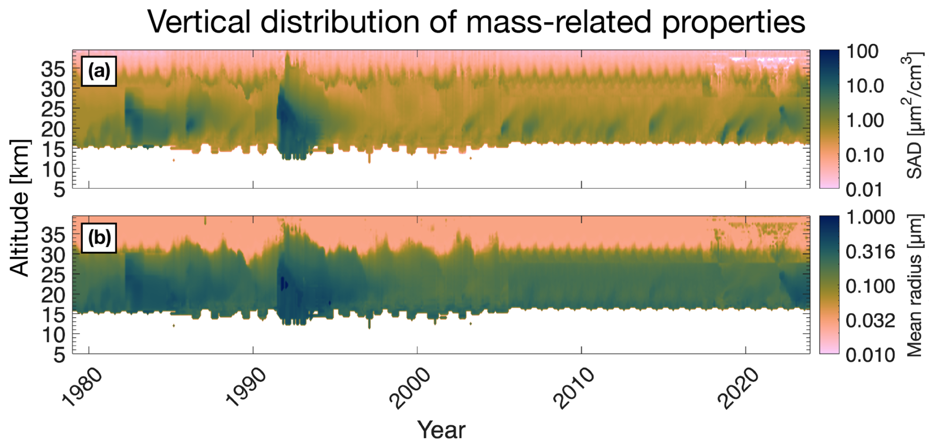
Figure 7 Surface area density (SAD) and mean radius for the time period 1979 and 2023 derived from the REMAP-GloSSAC-2023 record for the latitude band 0–5° N.

The values of SAD and r_mean are shown in Fig. 7 for the latitude band 0–5° N. During volcanically quiescent times, the stratospheric SAD is 0.5–1 µm² cm⁻³. After large volcanic eruptions, the SAD can reach 20–40 µm² cm⁻³.

3.4.2 Optical properties

In GCMs and CCMs, the optical properties AEC(λ), SSA(λ), and AF(λ) are required for each wavelength band to compute the radiative forcing exerted by the aerosol on the model. Some models need only the sulfate mass $m_{{\mathrm{H}}_{\mathrm{2}}{\mathrm{SO}}_{\mathrm{4}}}$ and from there estimate the radiation effects; therefore, for these models, we provided the total mass density of H₂SO₄ or other mass-related quantities as function of latitude, altitude, and time.

We provided these radiative properties for the CCMI-1, CMIP6, CCMI-2022, and HTHH-MOC models listed in Table 1, and they are openly available as SAGE-3λ (Luo, 2013), SAGE-4λ (Luo, 2017), REMAP-CCMI-2022-ref (Luo, 2020), REMAP-CCMI-2022-sai (Jörimann, 2023), and REMAP-GloSSAC-2023 (Jörimann, 2024) data sets (see “Data availability”).

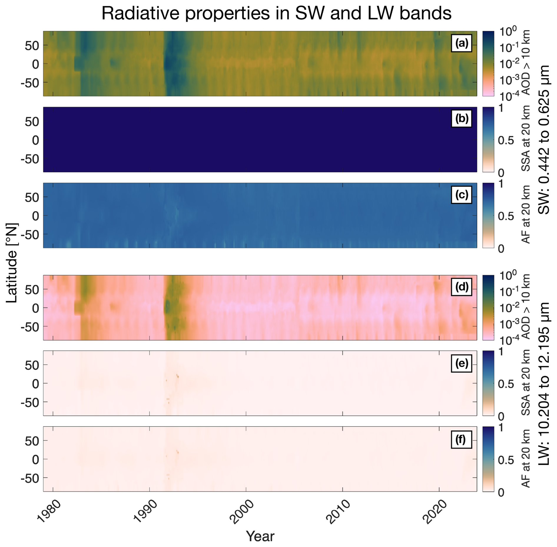
Figure 8 Aerosol radiative properties derived from REMAP-GloSSAC-2023: aerosol optical depth (AOD) above 10 km altitude and single-scattering albedo (SSA) and asymmetry factor (AF) at 20 km altitude from 1979 to 2023. (a–c) For one of the solar bands, the range is 0.442–0.625 µm of the ECHAM6 GCM. Panel (b) has constant data because all aerosol extinction is due to scattering, and for visible light there is no absorption at 20 km. (d–f) For one of the terrestrial bands, the range is 10.204–12.195 µm.

Figure 8 shows examples of AEC(λ), SSA(λ), and AF(λ) for two wavelength bands of the GCM ECHAM6. Figure 8a–c show the results for one solar band, 0.442–0.625 µm, and Fig. 8d–f for one terrestrial infrared band, 10.204–12.195 µm. The SSA in the visible band is unity by definition (assuming no absorption, i.e., only the real part of the refractive index matters). The backscattered solar radiation reduces the power of the incoming solar radiation, exerting an overall cooling. However, for the infrared band, 10–12 µm, the SSA is nearly zero. Then, the largest part of the extinction occurs due to absorption, which is why the stratospheric aerosol leads to in situ heating of the lower stratosphere.

3.5 Method using model output

For the CCMI-2022 sensitivity experiment senD2-sai, an aerosol forcing simulating human-made stratospheric aerosol injection (SAI) needed to be uniformly prescribed in different models (Plummer et al., 2021). The forcing was derived from a single-model ensemble run in the Whole Atmosphere Community Climate Model, version 2 of the Community Earth System Model (WACCM-CESM2). To apply REMAP to model output – instead of observations – the workflow was altered.

Instead of retrieving size distribution information, the output variables aerosol mode wet diameter and number density of the model's trimodal distribution were directly used for the Mie theory calculations. Relative humidity, temperature, and pressure fields were also readily available from the same source (cf. Table 1). For the three aerosol modes represented in WACCM-CESM2, we assumed a geometric standard deviation of σ = 1.6, σ = 1.6, and σ = 1.2, respectively. With these data, the AECs and the SSAs are readily calculated for any spectral band using Eqs. (5)–(8). The AF is given by Eqs. (9) and (10), while the mean radius and SAD are calculated with Eqs. (12) and (13), respectively.

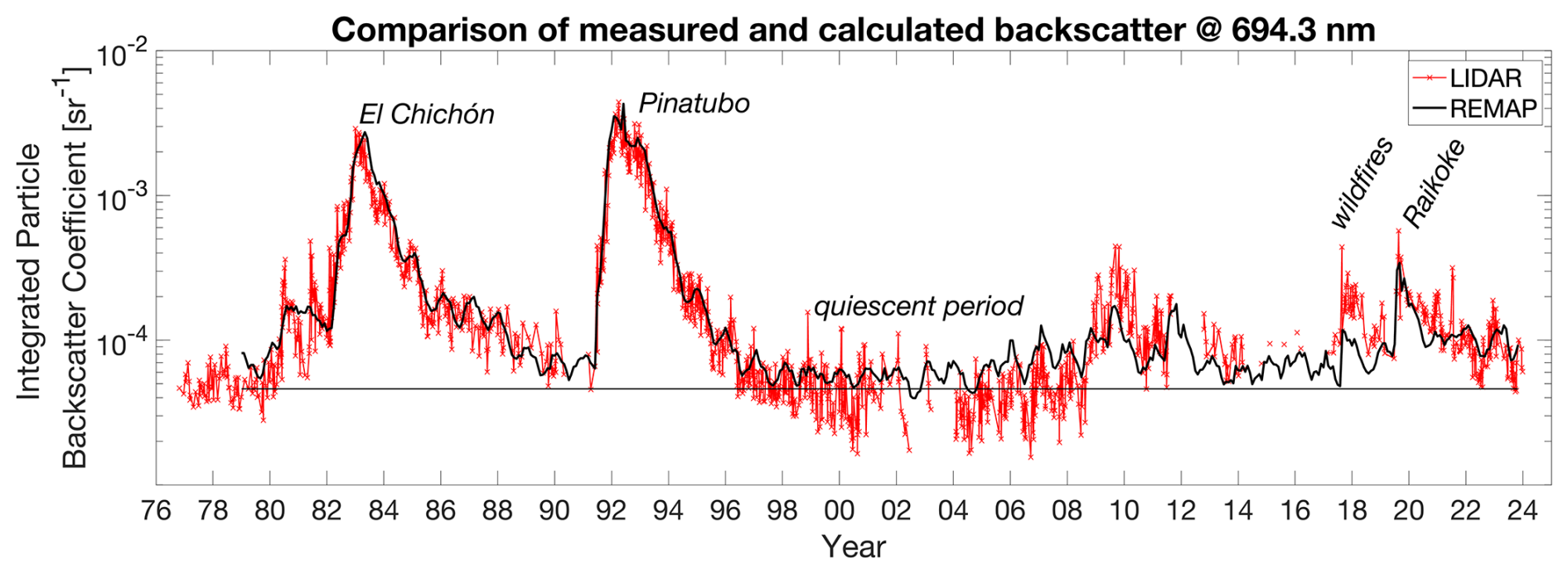
Figure 9 Integrated backscatter coefficients of stratospheric aerosol (integrated from 1 km above the tropopause to the upper end of the layer) over Garmisch-Partenkirchen, Germany (47.48° N, 11.06° E, 734 $\mathrm{m}\mathrm{a}.\mathrm{s}.\mathrm{l}.$). Red symbols and line: measured by the ground-based lidar at 694.3 nm. Several significant events are marked: the volcanic eruptions of El Chichón in 1982, Mount Pinatubo in 1991, and Raikoke in 2019; an extended quiescent period in 1997–2004; and the British Columbia (BC) wildfires. Data is from Trickl et al. (2023). Black line: zonal average monthly mean integrated backscatter coefficients for the latitude band from 45 to 50° N calculated from GloSSACv2.22 using REMAP with the parameterization σ(β₁₀₂₂) (Eq. 4).

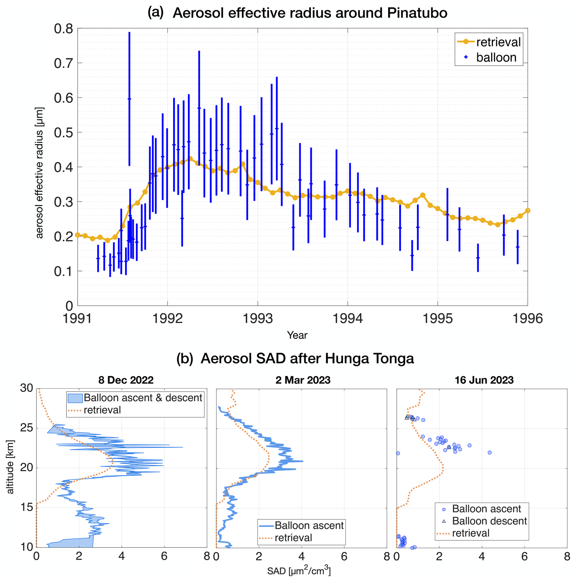
Figure 10 Comparison of balloon-borne measurements and REMAP monthly mean values retrieved using REMAP on GloSSAC. Panel (a) shows the mean aerosol effective radius averaged over 14–30 km altitude over Laramie, WY (41° N, 105° W), during the eruption of Mount Pinatubo in 1991, while panel (b) shows vertical surface area density (SAD) profiles over La Réunion (21° S, 55° E) after the Hunga Tonga–Hunga Ha`apai eruption (20° S, 175° W) in January 2022. The peak in SAD is the volcanic plume. For the retrieval, there are no data below the tropopause at around 15 km.

4 Validation

Recently, Trickl et al. (2023) published results of 45 years of ground-based lidar measurements of stratospheric aerosols since 1976 at the station Garmisch-Partenkirchen (47.5° N, 11.0° E, southern Germany). The integrated backscatter coefficients – a quantity required for SSAs – at 694.3 nm can also be calculated using the REMAP method. The agreement between the measured (red symbols and line in Fig. 9) and the calculated integrated backscatter coefficients (black line in Fig. 9) is very good. It should be noted that here we are comparing the zonal mean value of a 5° latitude band created with REMAP to the more fluctuating values from a single station. REMAP achieves excellent agreement after large volcanic eruptions (e.g., El Chichón in 1982, Mount Pinatubo in 1991, and Raikoke in 2020) but slightly underestimates the sustained volcanic burden in the episode of moderate volcanic eruptions around 2010. The retrieved integrated backscatter is also consistently high-biased in the background state (visible between 1997 and 2004), although other stations also report higher values than Garmisch-Partenkirchen in these years (Thomas Trickl, personal communication, 2024). We can trace this overestimation back to the lowest altitude levels in the stratosphere, where the single-mode lognormal distribution assumption does not hold and aerosol not dominated by sulfur is present, which cannot be correctly interpreted in REMAP. Large deviations in particular accordingly occur during large wildfires without any concurrent volcanic eruption, e.g., during and after the British Columbia wildfires (BC fires in Fig. 9) in 2018. In this comparison, even for these poorly captured events, the errors stay well within a factor of 2.

Since 1971, in situ particle measurements using an optical particle counter, OPC (Rosen and Kjome, 1991), combined with a condensation nuclei counter (CNC) (Delene and Deshler, 2000), have been performed on average twice a month at Laramie, Wyoming (41.3° N, 105.5° W, USA). The OPC measures the aerosol number density with radii r≳ 0.15 µm in several size channels. The CNC detects number density condensation nuclei with radii r≳ 10 nm. Uni- or bimodal lognormal aerosol size distributions have been obtained by fitting the measured counts of individual size channels of the OPC and CNC (Deshler et al., 2019). Quaglia et al. (2023) then calculated the effective radius as the ratio of the third and second moment of the obtained size distributions. Figure 10a shows mean aerosol effective radius after the Mount Pinatubo eruption (June 1991) between 14 and 30 km height above Laramie. Balloon measurements with 1 standard deviation are shown in blue and the corresponding REMAP values (37.5–42.5° N) in yellow. The momentary state of the stratosphere, measured by the balloons, fluctuates more than the monthly mean values captured by SAGE II, which the retrieval is mostly based on at this time. Regardless, the retrieved values mostly stay well within the measurement uncertainty range.

In Fig. 10b, measured and retrieved vertical profiles of aerosol SAD after the volcanic eruption of Hunga Tonga–Hunga Ha`apai (January 2022; 20° S, 175° W) are compared. The measured profiles are the result of the Balloon Baseline Stratospheric Aerosol Profiles (B²SAP) campaign (Todt et al., 2023) and were taken at La Réunion (21° S, 55° E, France) with Portable Optical Particle Spectrometers (POPSs), starting roughly a year after the eruption. The volcanic plume at this time is well mixed zonally and thus visible as elevated SAD between 20 and 25 km in both the balloon and retrieval data even though the longitudes of the eruption site and the balloon launch site are different. Below 15 km, no retrieval data are available because the troposphere is masked out, and thus the orange line is constant at zero. For the profile on 8 Dec 2022, measurements took place during both the ascent and descent of the balloon. The filled patch in light blue is bounded by these two profiles and illustrates the variability that the particle counter records during over slightly over a few hours of flight time. Since balloon campaigns see the momentary state of the atmosphere and the satellite-based retrieval operates on zonal monthly means, some discrepancies are expected to show up on account of short-term variability. Apart from those, both products agree well on the shape and height of the volcanic plume. For the 2 Mar 2023 profile, only the balloon ascent is available, which agrees well with the retrieval. The retrieval peak is roughly 25 % smaller than the OPC peak for this date, which again can be attributed to temporal and zonal averaging. For the 16 Jun 2023 profile, balloon data are scarce and show considerable scattering, and thus no conclusive comparison can be made for this date. More balloon data have been collected at other sites, and we offer an extended comparison, including background conditions, in the Supplement (Sect. S2).

5 Conclusions

The REMAP method is a useful tool for creating stratospheric aerosol forcings required as input for climate models and converting between different aerosol properties. The retrieval algorithm performs well under typical stratospheric conditions except near the tropopause and in regions with very low signal, typically close to the upper edge of the Junge layer. It has been used for studies on volcanic aerosol in the stratosphere and, more generally, to equip GCMs and CCMs in climate studies. The main limitation of the retrieval is the underlying assumption of a single-mode lognormal size distribution, which is necessary for REMAP to flexibly work on many different data sets with limited wavelength channels. Despite this limitation, REMAP also reproduces the particle size distributions after volcanic eruptions reasonably well. The Mie calculation is based on theoretical understanding and produces optical properties for each wavelength and for each wavelength band. The output parameter space and its resolution can be customized at the cost of computational time.

The backbone of all the stratospheric aerosol data sets created with REMAP for different MIPs are the SAGE II and III AECs at three and six wavelengths, respectively, which have provided the most complete coverage over multiple decades. These data are the basis for deriving important parameterizations that enable retrieval using only two or even one single channel, thus permitting the use of the GloSSAC composite. Between the end of the SAGE II and the beginning of the SAGE III operational period, there is a gap of over 10 years, meaning that no parameterization of similar quality can be established for this time. While OMPS-LP data are available starting in 2012, we have not used them with REMAP because of plans to integrate them into future GloSSAC versions (Kovilakam et al., 2024). Also, the limited accuracy of the OMPS (NASA) product reported by Taha et al. (2021) raises the question of whether sufficient quality wavelength channels would be available for retrieval. Currently, no other OMPS-LP product suited for use with REMAP exists. Therefore, we suggest using the SAGE III parameterization to bridge the gap, which we also used for the entire GloSSAC period, which is validated here.

The REMAP AECs calculated from the retrieved size distributions agree well with the measured data. This holds in not only the visible and near-infrared spectra (SAGE wavelengths at 525 (532 in SAGE III) nm and 1020 (1022) nm), but also the far-infrared spectrum (HALOE at 3.46 µm and ISAMS at 12.6 µm; see Fig. S3 to this paper for 3.46 µm and Fig. S6 of Arfeuille et al. (2013) for 12.6 µm). We also found good agreement with other observational data sets under background and volcanic conditions. We observed major systematic differences only from tropospheric intrusions from wildfires. We conclude that REMAP realistically reproduces the radiative (optical) and physical properties of the stratospheric aerosol, especially in the Junge layer. The main caveat is that the input data must be carefully selected and screened as biases of individual wavelengths and contaminated data points can significantly change the quality of the product. This includes assessing the measurement method and any assumptions made for data taking. Physical, mass-related properties retrieved using REMAP (notably surface area density and mean, median and mode radii) may be subject to larger errors under certain conditions. Even though we show in the Supplement (Sect. S4) that REMAP successfully reproduces AECs of both unimodal and bimodal size distributions, it is conceivable that for a bimodal aerosol, the retrieved size distribution parameters simply accurately recreate the optics but not necessarily all other properties. We suggest that for the satellite-based retrieval of stratospheric aerosol properties, the best way forward is to assimilate all of the available data and encourage the use of REMAP with the latest data releases to produce records and climate model input.