An extension of WeatherBench 2 to binary hydroclimatic forecasts

Binary forecasts of hydroclimatic extremes play a critical part in disaster prevention and risk management. While the recent WeatherBench 2 provides a versatile framework for verifying deterministic and ensemble forecasts of continuous variables, this paper presents an extension to binary forecasts of the occurrence versus non-occurrence of hydroclimatic extremes. Specifically, 17 verification metrics of the accuracy and discrimination of binary forecasts are employed and scorecards are generated to showcase the predictive performance. A case study is devised for binary forecasts of wet and warm extremes obtained from both deterministic and ensemble forecasts generated by three data-driven models, i.e., Pangu-Weather, GraphCast and FuXi, and two numerical weather prediction products, i.e., the high-resolution forecasting (HRES) and ensemble forecasting (ENS) of the Integrated Forecast System (IFS) of the European Centre for Medium-Range Weather Forecasts (ECMWF). The results show that the receiver operating characteristic skill score (ROCSS) serves as a suitable metric due to its relative insensitivity to the rarity of hydroclimatic extremes. For wet extremes, the GraphCast tends to outperform the IFS HRES when using the total precipitation of ERA5 reanalysis data as the ground truth. For warm extremes, Pangu-Weather, GraphCast and FuXi tend to be more skillful than the IFS HRES within 3 d lead time but become less skillful as lead time increases. In the meantime, the IFS ENS tends to provide skillful forecasts of both wet and warm extremes at different lead times and at the global scale. Through diagnostic plots of forecast time series at selected grid cells, it is observed that at longer lead times, forecasts generated by data-driven models tend to be smoother and less skillful compared to those generated by physical models. Overall, the extension of WeatherBench 2 facilitates more comprehensive comparisons of hydroclimatic forecasts and provides useful information for forecast applications.

1 Introduction

Accurate numerical weather prediction (NWP) is of great importance to the economy and society (Bi et al., 2023; Lam et al., 2023; Bauer et al., 2015). Conventionally, physical NWP models formulate the governing equations of coupled physical processes in the land, ocean and atmosphere and therefore predict weather conditions in the near future based on predetermined initial meteorological fields (Lam et al., 2023; Bauer et al., 2015). Due to advances in remote sensing, data assimilation and computational infrastructure, physical NWP models have witnessed steady improvements and been extensively employed in operational forecasting (Bauer et al., 2020). For example, the European Centre for Medium-range Weather Forecast (ECMWF) operates the Integrated Forecast System (IFS), which has implemented a remarkable resolution upgrade and methodology for high-resolution forecasting (HRES) and ensemble forecasting (ENS) at a horizontal resolution of 0.1° since January 2016 (Balsamo et al., 2023).

Data-driven NWP models have recently gained increasing popularity in hydroclimatic forecasting (Ben Bouallègue et al., 2024; Rasp et al., 2024; de Burgh-Day and Leeuwenburg, 2023; Xu et al., 2024a). Early models, such as the UNet-architecture-based cubed sphere projection (Weyn et al., 2020) and deep-Resnet-architecture-based models (Clare et al., 2021; Rasp and Thuerey, 2021), featured moderate spatio-temporal resolution and forecast skill. Recent deep learning models, such as the graph neural network (Keisler, 2022) and FourCastNet (Pathak et al., 2022), began to match operational NWP models in resolution and skills. Pangu-Weather (Bi et al., 2023) and GraphCast (Lam et al., 2023) even outperformed the HRES in terms of some deterministic metrics. The neural general circulation model (NeuralGCM), which integrates data-driven and physical modules, is considered to be the first hybrid model to obtain competitive or better scores than the HERS (Kochkov et al., 2024). GenCast generates global ensemble forecasts that are comparative or even more skillful than the ENS (Price et al., 2025).

There is a growing demand to verify the capability of physical and data-driven models in generating skillful hydroclimatic forecasts (Olivetti and Messori, 2024a; Zhong et al., 2024; Ben Bouallègue et al., 2024). In response to the need of a unified benchmark, WeatherBench has been established to host a common dataset of forecasts and observations and utilizes popular evaluation metrics for forecast comparisons (Rasp et al., 2020). Owing to rapid advances in data-driven NWP models, WeatherBench 2 has been developed to support global medium-range forecast verification (Rasp et al., 2024). By following the established practices of the World Meteorological Organization (WMO), WeatherBench 2 pays attention to both deterministic and ensemble forecasts of continuous variables generated by physical and data-driven NWP models (Jin et al., 2024). Forecast verification is performed by an open-source Python code and publicly available, cloud-optimized ground truth and baseline datasets (Jin et al., 2024; Olivetti and Messori, 2024b; Rasp et al., 2024).

Besides deterministic and ensemble forecasts of continuous variables, there is a demand for binary forecasts, i.e., categorical forecasts of binary events, in disaster prevention and risk management (Ben Bouallègue et al., 2024; Larraondo et al., 2020). Operational applications usually pay attention to the occurrence versus non-occurrence of certain hydroclimatic extremes instead of their precise magnitude (Larraondo et al., 2020; Rasp et al., 2020). Binary forecasts meet this demand by emphasizing the ability to capture hydroclimatic extremes, ensuring that models are not rewarded for merely minimizing average errors and generating unrealistically smooth forecasts (Ferro and Stephenson, 2011; Rasp et al., 2020). Therefore, this paper aims to extend WeatherBench 2 to binary forecasts. The objectives are (1) to account for verification metrics for binary forecasts derived from global precipitation and temperature forecasts, (2) to present scorecards to showcase the predictive performance with wet and warm extremes, and (3) to examine the sensitivity of different metrics to predefined thresholds of hydroclimatic extremes. As is shown in the methods and results, the extension facilitates an effective intercomparison among binary forecasts of hydroclimatic extremes generated by both data-driven and physically based models.

2 Forecasts and metrics in WeatherBench 2

2.1 Forecast datasets

WeatherBench 2 presents a benchmark for verifying and comparing the performance of data-driven and physical NWP models (Rasp et al., 2024). On its website (https://weatherbench2.readthedocs.io, last access: 20 August 2025), there is a database containing past forecasts in the year 2020:

1. The HRES generated by the ECMWF's IFS is widely regarded as one of the best global deterministic weather forecasts (Rasp et al., 2024). It offers 10 d forecasts at a horizontal resolution of 0.1° with 137 vertical levels (Balsamo et al., 2023). In WeatherBench 2, the HRES is primarily used as the baseline for comparing the performance of data-driven models.

2. The ENS generated by the IFS's ensemble version is widely known as one of the best global ensemble weather forecasts. It consists of 1 control member and 50 perturbed members (Balsamo et al., 2023). In WeatherBench 2, the ENS also serves as an important baseline, with a mean value of the 50 members, i.e., ENS Mean, being extensively used (Rasp et al., 2024).

3. The 10 d global forecasts generated by Pangu-Weather consist of 5 upper-air variables at 13 vertical levels and 4 surface variables at the horizontal resolution of 0.25° (Bi et al., 2023). Pangu-Weather is based on the vision transformer architecture and hierarchical temporal aggregation. Four time steps, i.e., 1, 3, 6 and 24 h, are chained autoregressively to generate forecasts at any lead time based on the current atmospheric states. It is noted that two sets of Pangu-Weather forecasts, which are respectively based on the ERA5 and HRES initializations, are generated (Rasp et al., 2024).

4. The 10 d forecasts generated by GraphCast include 6 upper-air variables at a maximum of 37 vertical levels and 5 surface variables at a horizontal resolution of 0.25° (Lam et al., 2023). The GraphCast is based on the architecture of the graph neural network. It runs autoregressively to forecast atmospheric states for the next time step based on states from the previous two time steps at a temporal resolution of 6 h. Similarly, there are two sets of GraphCast forecasts generated from the ERA5 and HRES initializations (Rasp et al., 2024).

5. The 15 d global forecasts generated by FuXi consist of 5 upper-air variables at 13 vertical levels and 5 surface variables at a horizontal resolution of 0.25° (Chen et al., 2023). FuXi is an autoregressively cascading model based on U-Transformer architecture. It consists of three sub-models fine-tuned for forecasting 0–5, 5–10 and 10–15 d ahead at a temporal resolution of 6 h. Atmospheric states are forecasted based on states from the previous two time steps.

2.2 Verification metrics

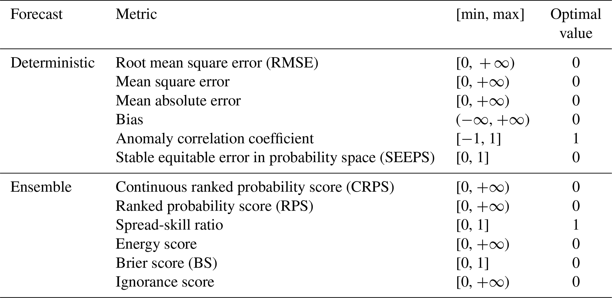
In total, WeatherBench 2 takes into consideration six metrics for deterministic forecasts and six metrics for ensemble forecasts, as shown in Table 1. The ERA5 reanalysis data are used as the ground truth for verifying the data-driven models. For the sake of fair comparison with the data-driven models, the initial conditions of the IFS HRES are used as the ground truth for the verification of IFS forecasts (Lam et al., 2023). As precipitation is not available for the IFS HRES's initial conditions, the total precipitation of ERA5 reanalysis data is used as the ground truth data for all models. Following the initial version of WeatherBench 2, the verification is conducted for forecasts initialized at 00:00 and 12:00 UTC for the period from 1 January to 31 December 2020. All forecasts, baseline data and ground truth data are resampled to a horizontal resolution of 1.5°, which is used as the standard resolution for forecast verification by the WMO and ECMWF (Rasp et al., 2024).

Table 1 Verification metrics for deterministic and ensemble forecasts of continuous variables in WeatherBench 2.

3 Verification of binary hydroclimatic forecasts

3.1 Conversion to binary forecasts

Binary forecasts of the occurrence versus non-occurrence of target events can be generated from deterministic and ensemble forecasts of continuous variables by using predefined thresholds of hydroclimatic events (Ben Bouallègue et al., 2024). In operational applications, binary forecasts of extreme precipitation events and heat waves can respectively be derived from precipitation and temperature forecasts (Huang and Zhao, 2022; Lang et al., 2014; Zhao et al., 2022; Slater et al., 2023). As for the precipitation, the 90th percentile of the 24 h accumulation of total precipitation (TP24h) is considered to be the threshold, above which TP24h is considered to be the wet extreme (North et al., 2013; Xiong et al., 2024). As to temperature, the 90th percentile of the 24 h maximum of 2 m temperature (T2M24h) is set as the threshold, above which T2M24h is categorized as the warm extreme (Xiong et al., 2024; Zhao et al., 2024). It is noted that the thresholds in each grid cell are separately calculated (Olivetti and Messori, 2024b). Given the predefined threshold q, deterministic forecasts are converted into either 0 or 1:

$$\begin{array}{}\text{(1)}& I\left(f_n>q\right)=\left\{\begin{array}{ll}\mathrm{1},& f_n>q\\ \mathrm{0},& \mathrm{otherwise}\end{array}\right.,\end{array}$$

where f_n represents the nth deterministic forecast. In the meantime, ensemble forecasts are converted into forecast probabilities using Weibull's plotting position (Makkonen, 2006):

$$\begin{array}{}\text{(2)}& p_{f_n}={\displaystyle \frac{\sum _{m=\mathrm{1}}^{M}I\left(f_{n,m}>q\right)}{M+\mathrm{1}}},\end{array}$$

where f_n,m is the mth member of the nth ensemble forecast, and M is the number of ensemble members.

The contingency table plays a key part in the verification of binary forecasts of hydroclimatic events (Larraondo et al., 2020). As shown in Table 2, there are four parts of the contingency table, i.e., true positives (a), false positives (b), false negatives (c) and true negatives (d). Specifically, the true positives indicate that target occurrences are successfully forecasted; the false positives indicate non-occurrences incorrectly forecasted as occurrences; the false negatives indicate target occurrences incorrectly forecasted as non-occurrences; the true negatives indicate non-occurrences that are correctly forecasted as non-occurrences. The proportion of the observed occurrences to the total number of occurrences and non-occurrences is the base rate ($(a+c)/N$), with lower values often corresponding to events that are more extreme (Ferro and Stephenson, 2011).

Table 2 Contingency table for binary forecasts.

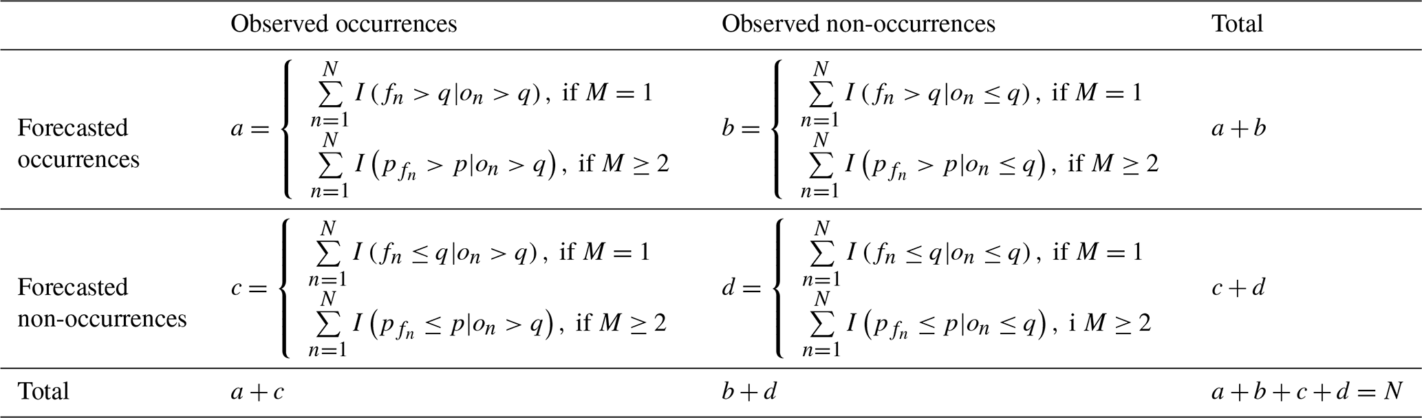
Where M=1 and M≥2 respectively represent deterministic and ensemble forecasts; N is the number of pairs of observations and forecasts for verification; o_n represents the nth observation; p denotes the probability thresholds above which the occurrences are forecasted to occur for ensemble forecasts; I( ) denotes the indicator function.

3.2 Verification metrics for binary forecasts

Given the challenges posed by varying hydroclimatic extremes and imbalanced samples, in total 17 metrics are utilized to examine the performance of binary forecasts (Jolliffe and Stephenson, 2012; North et al., 2013). Notably, there are eight base-rate-dependent metrics and nine base-rate-independent metrics. On the one hand, the base-rate-dependent metrics facilitate insights into the performance in relation to varying frequency of extreme events (Jolliffe and Stephenson, 2012). On the other hand, the base-rate-independent metrics are applicable for comparing forecasts across different climate regions or time periods, in which the frequency of extreme events differs substantially (Ferro and Stephenson, 2011; Jacox et al., 2022). Their equations, ranges and optimal values are presented in Table 3.

Table 3 Verification metrics for binary forecasts.

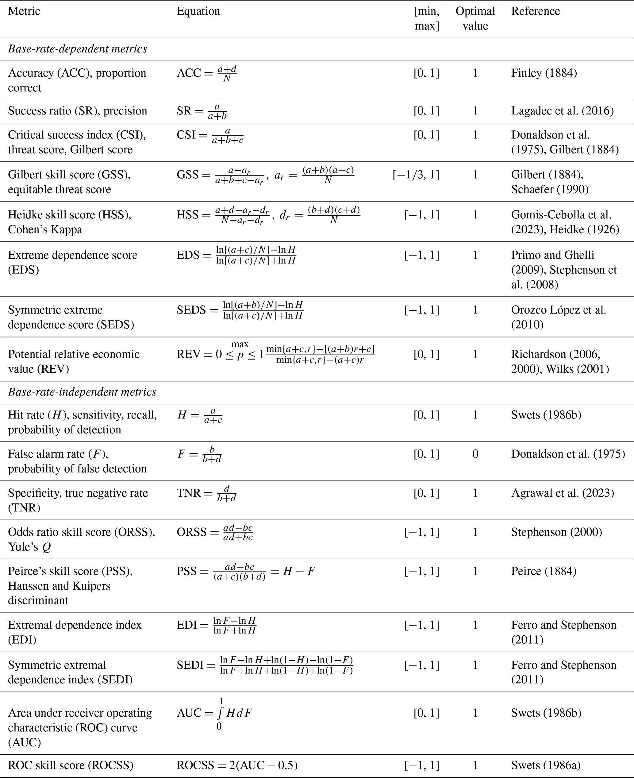
The variables a, b, c and d respectively denote the number of true positives, false positives, false negatives and true negatives, with the equations shown in Table 2; N is the number of pairs of observations and forecasts; p denotes the probability thresholds above which the occurrences are forecasted to occur for ensemble forecasts; r represents the cost–loss ratio for calculating the relative economic value; all calculation equations of other variables can be found in this table.

The eight base-rate-dependent metrics in Table 3 are influenced by the underlying distribution of observed occurrences and non-occurrences (Jolliffe and Stephenson, 2012). The accuracy is calculated as the ratio between the number of true positives and the total number of occurrences and non- occurrences (Finley, 1884). The success ratio (SR) measures the number of true positives divided by the number of forecasted occurrences (Lagadec et al., 2016). The critical success index (CSI) is the number of true positives divided by the total number of forecasted and observed occurrences (Chakraborty et al., 2023; Gilbert, 1884; Donaldson et al., 1975). The Gilbert skill score (GSS) evaluates the fraction of true positives over the observed and forecasted occurrences after adjusting for the random true positives (Chen et al., 2018; Coelho et al., 2022). The Heidke skill score (HSS) measures the accuracy relative to that of the random forecasts (Gomis-Cebolla et al., 2023). The extreme dependency score (EDS) (Stephenson et al., 2008) and the symmetric extreme dependency score (SEDS) (Orozco López et al., 2010) can measure the general performance of binary forecasts for rare events. The potential relative economic value (REV) quantifies the potential value of a forecast over a range of different probability thresholds (p) to make a decision (Richardson, 2006, 2000; Wilks, 2001). It compares the saved expense using the forecasts instead of climatology relative to the saved expense using the perfect forecast (Price et al., 2025).

The nine base-rate-independent metrics in Table 3 are valuable for rare events due to their stability with respect to the variation in the proportion of observed occurrences (Ferro and Stephenson, 2011). The hit rate and false alarm rate respectively quantify the proportion of true positives in observed occurrences and the proportion of false positives in observed non-occurrences (Swets, 1986b). The specificity measures the percentage of true negatives to observed non-occurrences (Agrawal et al., 2023). The odds ratio skill score (ORSS) examines the improvement over the random forecasts, emphasizing the balance between positive and negative samples (Stephenson, 2000). Peirce's skill score (PSS) has a similar formulation to HSS but does not depend on occurrence frequency (Chakraborty et al., 2023). For deterministic forecasts, the PSS equals the maximum value of REV when the cost–loss ratio equals the base rate (Richardson, 2006). The extremal dependence index (EDI) and the symmetric extremal dependence index (SEDI) are designed to be nondegenerate to measure the predictive performance for rare events (Ferro and Stephenson, 2011). The receiver operating characteristic (ROC) examines the discrimination between true positives and false positives, quantified by the area under the ROC curve (AUC) (Swets, 1986b). The ROC skill score (ROCSS) compares the discriminative ability over random forecasts.

Among the 17 metrics, the ROCSS is base-rate-independent and suitable for both deterministic and probabilistic forecasts of binary events. By contrast, the other metrics need some predefined probability thresholds to convert probabilistic forecasts into deterministic forecasts. Therefore, the ROCSS is selected as the primary verification metric in the analysis. For probabilistic forecasts, the ROCSS is calculated by considering the hit rates and false alarm rates for all possible thresholds of probability (Huang and Zhao, 2022). It is noted that higher ROCSS values indicate better forecast skill.

3.3 Forecast verification

Considering data availability and forecast settings, the verification focuses on eight sets of forecasts: IFS's HRES, ENS and ENS Mean; operational forecasts from Pangu-Weather and GraphCast; and hindcasts from Pangu-Weather, GraphCast and FuXi. The ground truth, spatial resolution, initial forecast time and verification period are selected by following WeatherBench 2. A set of predefined thresholds ranging from the 80th to 99th percentiles of the ground truth data in 2020 are considered for sensitivity analysis (Olivetti and Messori, 2024b; North et al., 2013). For comparison in individual grid cells, the 17 metrics are computed one by one. Furthermore, the 17 metrics are calculated using the area-weighting method for the regions predetermined by the ECMWF's scorecards, as shown in Table 4 (Rasp et al., 2024).

Table 4 Regions that are included in the ECMWF's scorecards.

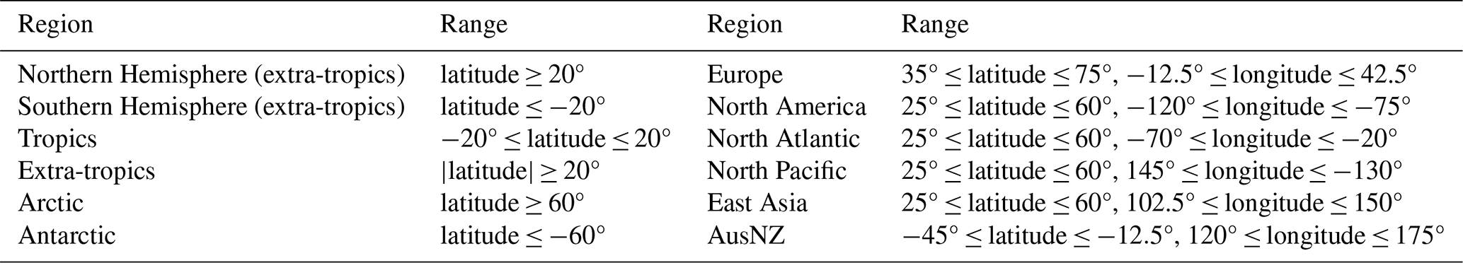
AusNZ: Australia and New Zealand.

Considering that hydroclimatic observations are subject to heteroscedasticity and autocorrelation due to spatial and temporal clustering of hydroclimatic extremes (Olivetti and Messori, 2024b), the cluster-robust standard errors are used to correct the paired t test (Liang and Zeger, 1986; Shen et al., 1987). Specifically, the corrected two-sided paired t test is performed at a significance level of 0.05 to assess the differences in the performance between data-driven models and IFS HRES (Olivetti and Messori, 2024b). For comparison in individual grid cells, the same paired t test is performed with a p value that is corrected for multiple testing using global false-discovery rates at a significance level of 0.1 (Benjamini and Hochberg, 1995; Olivetti and Messori, 2024b). This setting corresponds to a significance level of 0.05 for spatially correlated hydroclimatic extremes (Wilks, 2016).

4 Results

4.1 Predictive performance across the globe

Scorecards of the globally area-weighted ROCSS relative to the IFS HRES baseline are shown in Fig. 1. As expected, forecasts become less skillful as lead time increases from 1 to 10 d. This outcome is in general due to the accumulation of forecast errors over time caused by the autoregressive architecture of these models (Olivetti and Messori, 2024b; Bonavita, 2024). For wet extremes, the IFS ENS, IFS ENS Mean, GraphCast (operational) and GraphCast tend to outperform the IFS HRES. At lead times of 3 and 10 d, the ROCSS is respectively 0.59 and 0.16 for the IFS HRES, 0.90 and 0.55 for the IFS ENS, 0.61 and 0.17 for the IFS ENS Mean, 0.65 and 0.20 for GraphCast (operational), 0.61 and 0.16 for GraphCast, and 0.54 and 0.08 for FuXi. For warm extremes, GraphCast and FuXi tend to be more skillful than the IFS HRES within 3 d lead time. As lead time increases, data-driven forecasts are generally less skillful than the IFS HRES. This result is not surprising since the over-smoothing is observed to be more prominent among data-driven models than physical models (Bonavita, 2024; Lam et al., 2023). It is highlighted that the IFS ENS is remarkably more skillful than the IFS HRES at lead times from 1 to 10 d. At lead times of 3 and 10 d, the ROCSS is respectively 0.68 and 0.42 for the IFS HRES, 0.92 and 0.86 for the IFS ENS, 0.62 and 0.32 for the IFS ENS Mean, 0.63 and 0.29 for Pangu-Weather, 0.68 and 0.39 for GraphCast, and 0.68 and 0.32 for FuXi.

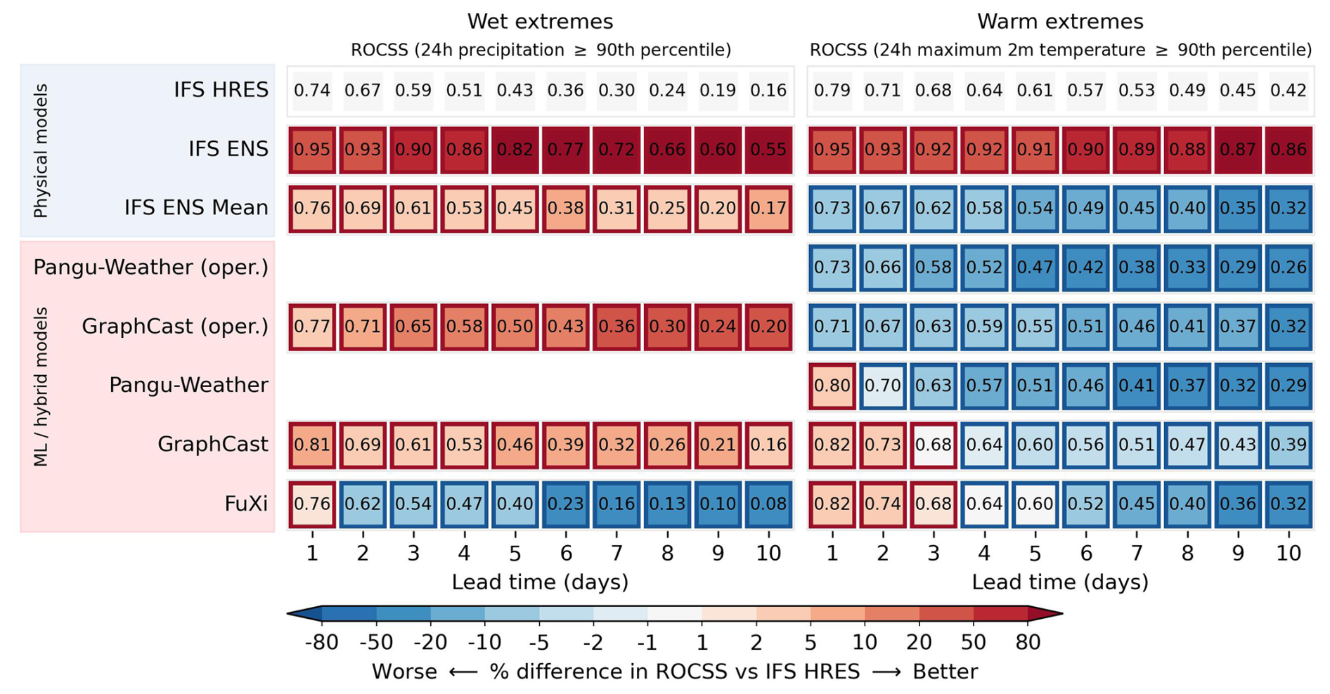
Figure 1 Globally area-weighted ROCSS for wet and warm extremes. “Oper.” denotes the operational version. The red and blue borders indicate significantly different performances compared to the IFS HRES at the significance level of 0.05.

Scorecards of the area-weighted ROCSS for wet extremes relative to the IFS HRES baseline are illustrated by region in Fig. 2. Overall, the IFS ENS stands out across different regions and lead times. The operational version of GraphCast tends to be better than the IFS HRES across different regions. The raw version of GraphCast tends to be better than the IFS HRES except for in the Northern Hemisphere (extra-tropics), the tropics, the extra-tropics, North America and the North Atlantic. In Europe, at lead times of 3 and 10 d, the ROCSS is respectively 0.73 and 0.19 for the IFS HRES, 0.96 and 0.64 for the IFS ENS, 0.76 and 0.23 for GraphCast (operational), 0.77 and 0.22 for GraphCast, and 0.69 and 0.11 for FuXi. In the meantime, the FuXi tends to outperform the IFS HRES in the Southern Hemisphere (extra-tropics), tropics, North Atlantic and AusNZ at lead time less than 3 d. Except for the Arctic and Antarctic, the IFS ENS Mean tends to be better than the IFS HRES. GraphCast (operational) is comparable to the IFS ENS Mean and marginally better in the polar regions. In the Antarctic region, the ROCSS is 0.63 and 0.06 for the IFS HRES, 0.59 and 0.01 for the IFS ENS Mean, and 0.66 and 0.06 for GraphCast (operational) at lead times of 3 and 10 d.

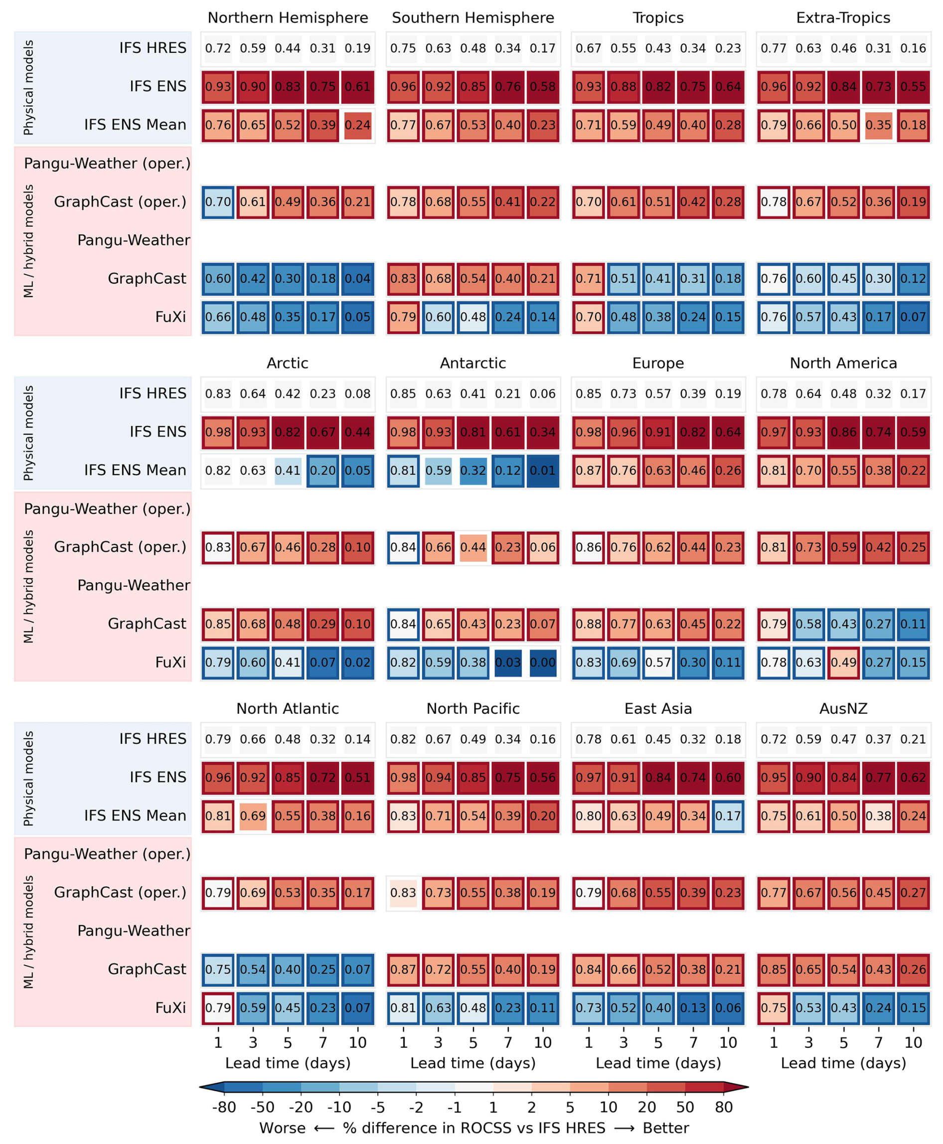
Figure 2 Regionally area-weighted ROCSS of different forecasts for wet extremes. The red and blue borders indicate significantly different performance compared to the IFS HRES at the significance level of 0.05.

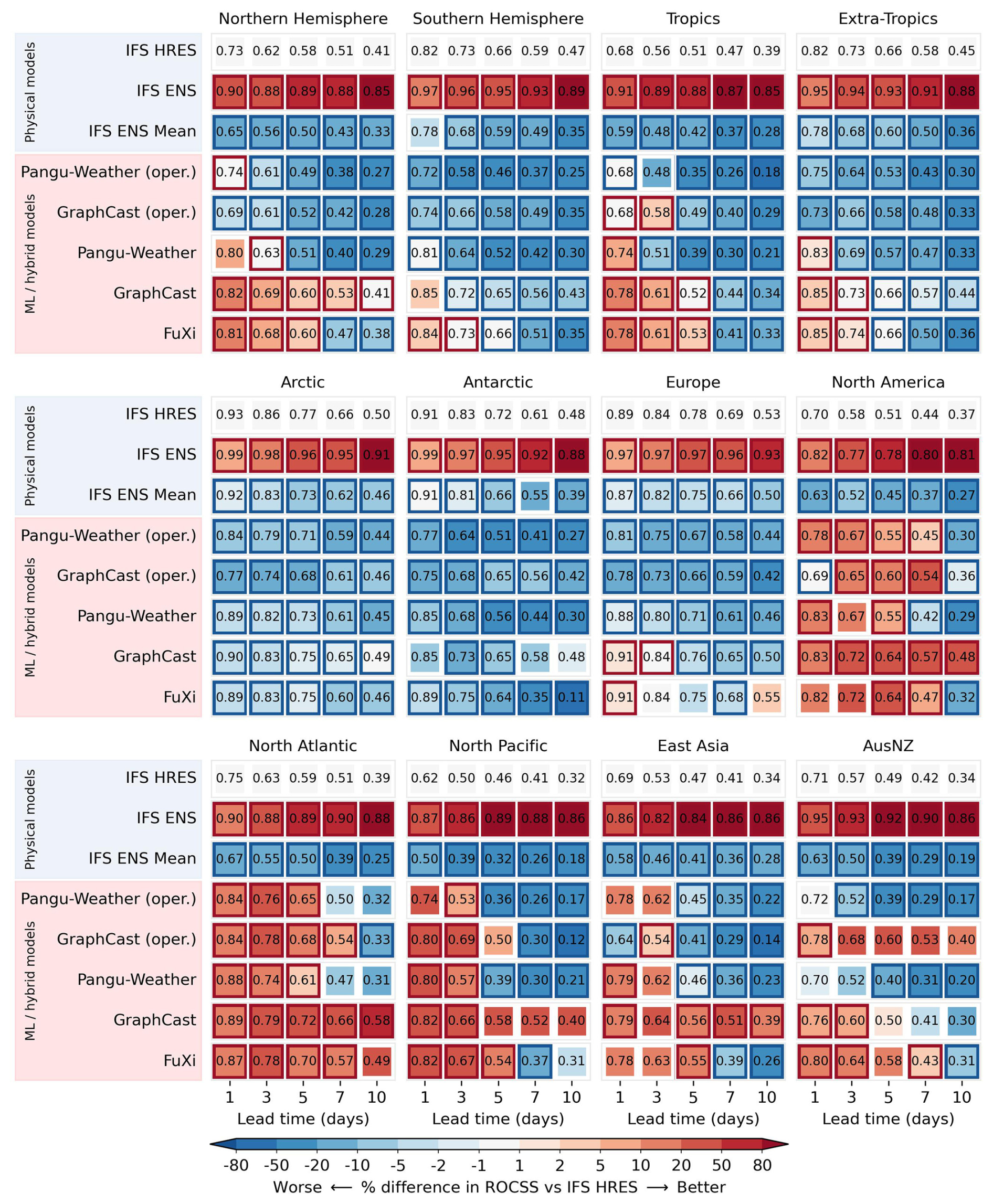
Scorecards of the regionally area-weighted ROCSS for warm extremes relative to the IFS HRES baseline are showcased in Fig. 3. Pangu-Weather, GraphCast and FuXi tend to outperform the IFS HRES within 3 d lead time except for in the Arctic and Antarctic. These results are consistent with the results of a previous study on forecast accuracy of the magnitude for warm extremes (Olivetti and Messori, 2024b). In North America, the North Atlantic, the North Pacific, East Asia and AusNZ, GraphCast and FuXi tend to outperform the IFS HRES at longer lead times even up to 10 d. The ROCSS in the North Atlantic is respectively 0.39, 0.58 and 0.49 for the IFS HRES, GraphCast and FuXi at a 10 d lead time. On the other hand, the performances of all data-driven forecasts tend to be worse than that of the IFS HRES in the Arctic and Antarctic. In Europe, the ROCSS is respectively 0.78, 0.71, 0.76 and 0.75 for the IFS HRES, Pangu-Weather, GraphCast and FuXi at a 5 d lead time. As averaging the ensemble members can filter unpredictable features to get smoother forecasts, it is not surprising that the IFS ENS Mean does not always perform as well as the IFS HRES and IFS ENS for warm extremes (Ben Bouallègue et al., 2024).

Figure 3 As for Fig. 2, but for warm extremes.

4.2 Predictive performance of wet extremes

The differences in the ROCSS for wet extremes in comparison to the IFS HRES baseline are illustrated in Fig. 4. Overall, the IFS ENS tends to outperform the IFS HRES in most grid cells across the globe. Except for northern Africa and the Arabian Peninsula, GraphCast's operational forecasts are comparable to or more skillful than the IFS HRES. GraphCast is not as skillful as the IFS HRES in more grid cells, such as northern Africa, central Australia and central Asia. FuXi tends to be less skillful than the IFS HRES in most grid cells, such as northern Africa, the Atlantic and the Pacific. As the lead time increases, the IFS ENS and GraphCast (operational) are observed to outperform the IFS HRES, while GraphCast and FuXi underperform. These results are consistent with the results of Figs. 1 and 2. In northern Africa, forecasts of the three data-driven models tend to be less skillful than the IFS HRES and IFS ENS. As GraphCast and FuXi exhibit no hits and so many false positives for many or even almost all of the grid cells in this region, the ROCSS is nearly −1 so that their forecasts tend to be worse than the IFS HRES in the Northern Hemisphere (extra-tropics) and tropics.

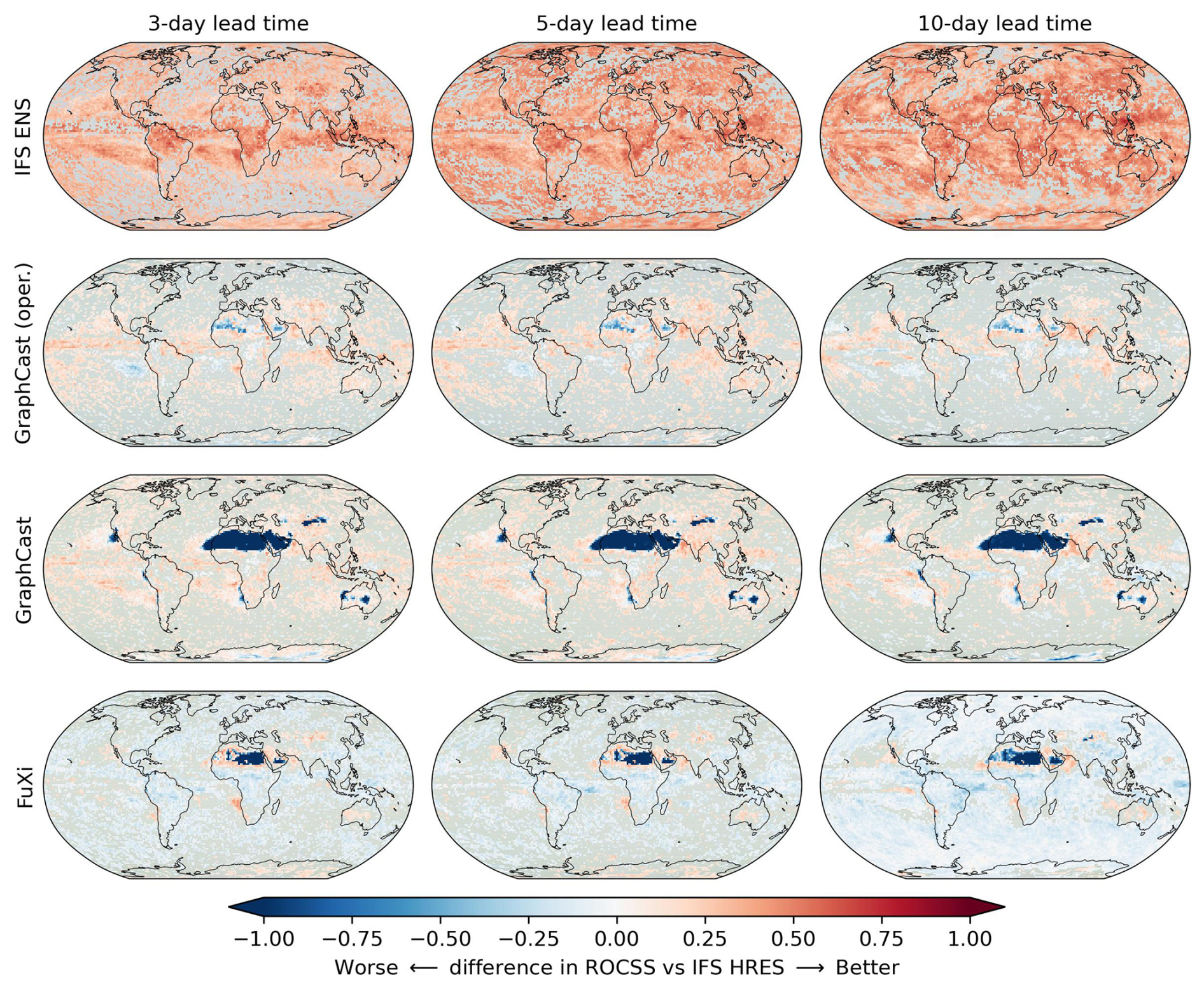
Figure 4 Differences between IFS ENS, GraphCast (operational), GraphCast and FuXi in ROCSS and the IFS HRES for wet extremes in each grid cell. The gray color indicates grids with no statistically significant differences at the significance level of 0.1.

The time series for 24 h accumulation of total precipitation from different forecasts initialized at 00:00 UTC are shown for three grid cells in Fig. 5. The grid cells A, B and C are selected respectively due to the better, close and worse performance of data-driven models relative to the IFS HRES. Overall, data-driven models can capture the temporal dynamics of precipitation, but their forecasts are smoother than the IFS HRES (Zhong et al., 2024; Xu et al., 2024b). For grid cells A and B, the five sets of forecasts have nearly an equal number of true negatives; the IFS HRESs show more true positives but more false negatives; GraphCast is more capable of capturing the wet extremes but tends to produce more false positives; and the IFS ENS Mean and FuXi tend to underestimate the wet extremes, resulting in more false negatives but fewer false positives. For grid cell C, located in northern Africa, GraphCast and FuXi tend to overestimate the low precipitation and underestimate the high precipitation, leading to zero numbers of true negatives for FuXi and zero numbers of false negatives for both. At lead times of 3 and 10 d, the ROCSS is respectively 0.48 and 0.09 for the IFS HRES, 0.80 and 0.53 for the IFS ENS, 0.31 and 0.21 for the operational GraphCast, −0.94 and −0.96 for GraphCast, and −1.00 and −1.00 for FuXi.

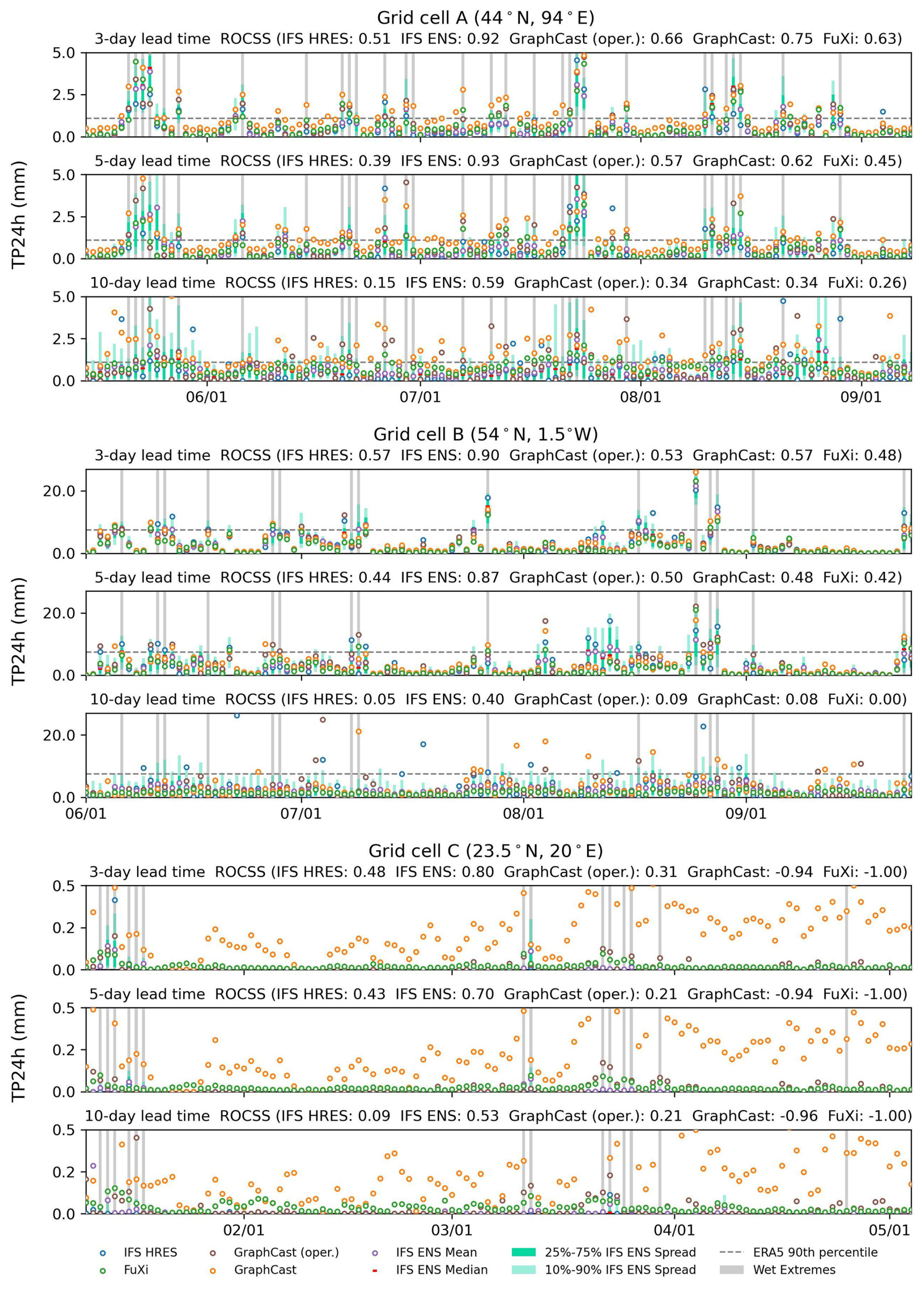
Figure 5 Time series plots of TP24h forecasts initialized at 00:00 UTC for the IFS HRES, IFS ENS, IFS ENS Mean, GraphCast and FuXi over three selected grid cells, i.e., A (44° N, 94° E), B (54° N, 1.5° W) and C (23.5° N, 20° E).

4.3 Predictive performance of warm extremes

The differences in ROCSS for warm extremes in comparison to the IFS HRES baseline are illustrated in Fig. 6. The IFS ENS tends to outperform the IFS HRES, especially in low-latitude regions. As the lead time increases, the IFS ENS tends to be more skillful than the IFS HRES. The ROCSS of Pangu-Weather, GraphCast and FuXi is similar to that of the IFS HRES but is lower in most grids of the Pacific, Atlantic and Arctic. GraphCast tends to outperform the IFS HRES in the North Atlantic near the Gulf of Mexico. The spatial patterns of the differences in ROCSS are consistent with the results of Fig. 3. As the lead time increases to 10 d, the area where Pangu-Weather, GraphCast and FuXi are more skillful than the IFS HRES decreases. On the other hand, even for a lead time of 10 d, GraphCast and FuXi continue to outperform the IFS HRES in some regions of the North Atlantic. The different performances of global weather forecasts in different regions emphasize the necessity to verify and calibrate hydroclimatic forecasts before operational application (Ben Bouallègue et al., 2024; Huang et al., 2022).

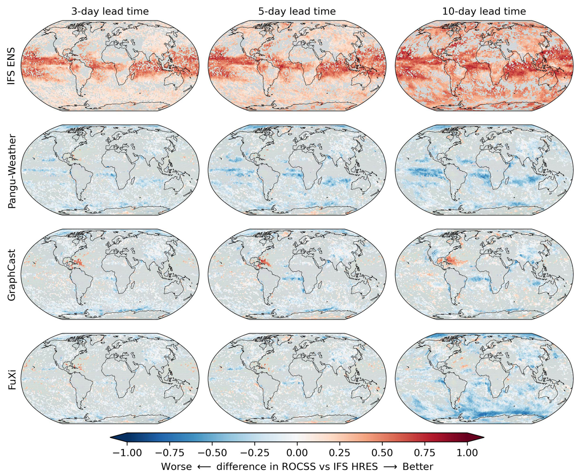
Figure 6 Differences between IFS ENS, Pangu-Weather, GraphCast and FuXi in ROCSS and the IFS HRES for warm extremes in each grid cell. The gray color indicates grids with no statistically significant differences at the significance level of 0.1.

The time series for the 24 h maximum of 2 m temperature from different forecasts initialized at 00:00 UTC are shown for three grid cells in Fig. 7. The grid cells D, E and F are also selected respectively due to the better, close and worse performance of data-driven models relative to the IFS HRES. Overall, Pangu-Weather, GraphCast and FuXi exhibit similar temperature dynamics over time to those of the IFS HRES. For grid cell D, Pangu-Weather, GraphCast and FuXi tend to outperform the IFS HRES. Pangu-Weather tends to underestimate the temperature, leading to fewer true positives and more false negatives. GraphCast and FuXi show more true positives. For grid cell E, these models show a nearly equal number of true positives and true negatives, resulting in similar ROCSS. For grid cell F, the data-driven models tend to be less accurate than the IFS HRES. Pangu-Weather, GraphCast and FuXi tend to underestimate the temperature, leading to more false negatives and fewer true positives. As the lead time increases from 3 to 10 d, the ROCSS reduces from 0.48 to 0.28 for Pangu-Weather, from 0.51 to 0.22 for GraphCast and from 0.54 to 0.17 for FuXi. By contrast, the IFS HRES and IFS ENS change less. The ROCSS decreases from 0.76 to 0.56 for the IFS HRES and from 0.95 to 0.86 for the IFS ENS.

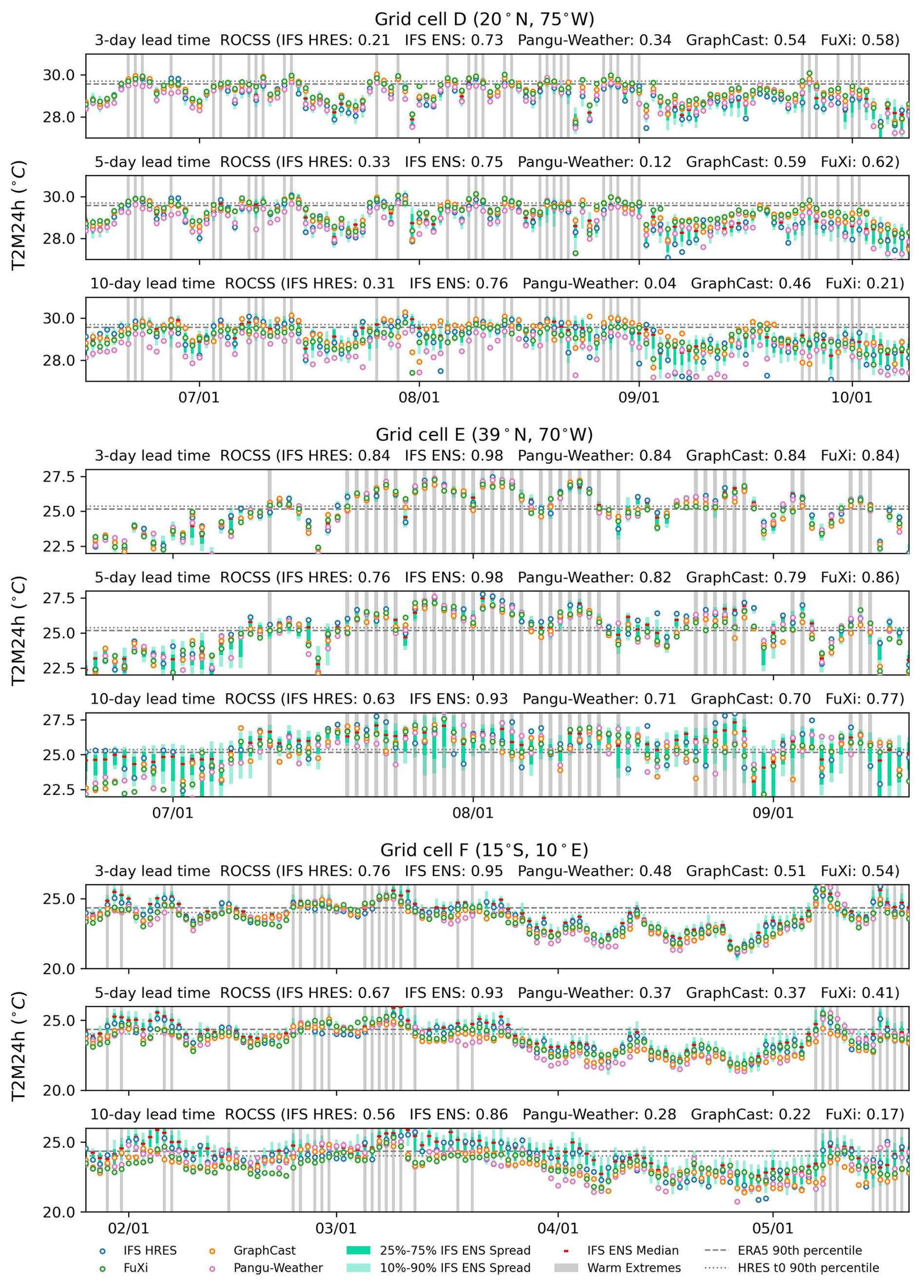
Figure 7 Time series plots of T2M24h forecasts initialized at 00:00 UTC for the IFS HRES, IFS ENS, Pangu-Weather, GraphCast and FuXi over three selected grid cells, i.e., D (20° N, 75° W), E (39° N, 70° W) and F (15° S, 10° E).

4.4 Sensitivity to predefined thresholds

The globally area-weighted performance under different predefined thresholds is illustrated for 5 d lead time in Fig. 8. The ROCSS is base-rate-independent and simultaneously suitable for deterministic and probabilistic forecasts of binary events. It is noted that the REV needs predefined cost–loss ratios to calculate the potential values of forecasts, while the cost–loss ratios may be different for hydroclimatic extremes with different threshold percentiles. In the meantime, the SEDI is also applicable to extreme events because of its base-rate independence and nondegenerate limit (North et al., 2013; Jolliffe and Stephenson, 2012; Brodie et al., 2024). The base-rate-independent metrics change little as the predefined thresholds increase from the 80th to the 99th percentile. Specifically, as for forecasting wet extremes at a 5 d lead time, the scores of GraphCast decrease from 0.74 to 0.56 for SEDI and from 0.43 to 0.23 for ROCSS as the thresholds increase from the 80th to the 99th percentile. By contrast, the scores of GraphCast increase from 0.81 to 0.98 for 1-BS, from 0.87 to 0.95 for ORSS and from 0.51 to 0.52 for SEDS. These metrics are not suitable for hydroclimatic extremes because they contradict the notion that rarer events are often more difficult to predict (Ferro and Stephenson, 2011).

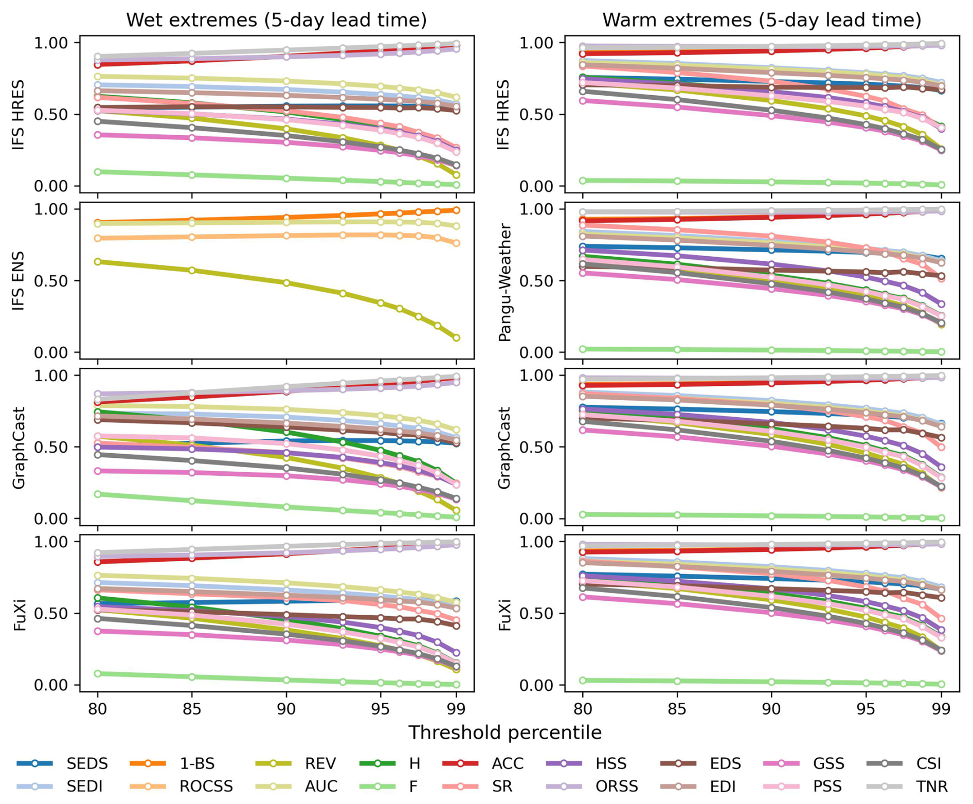
Figure 8 Globally area-weighted performance in forecasting wet extremes and warm extremes with different threshold percentiles at 5 d lead time. The REV is calculated with a fixed cost–loss ratio of 0.2 only for purposes of illustration.

The globally area-weighted ROCSS under different predefined thresholds and lead times is shown in Fig. 9. Overall, the ROCSS decreases for all eight sets of forecasts as the predefined thresholds increase from the 80th to the 99th percentile. The IFS ENS tends to perform better in forecasting wet extremes and warm extremes. Among the available data-driven models, GraphCast (operational) tends to be more skillful for wet extremes; for warm extremes, FuXi tends to be more skillful at lead times less than 5 d, and GraphCast tends to be better at lead times more than 5 d. Specifically, as for forecasting wet extremes at a 5 d lead time, the ROCSS decreases from 0.46 to 0.24 for IFS HRES, from 0.80 to 0.77 for IFS ENS and from 0.53 to 0.26 for GraphCast (operational). As for forecasting warm extremes at a 5 d lead time, the ROCSS decreases from 0.69 to 0.41 for IFS HRES, from 0.93 to 0.83 for IFS ENS and from 0.70 to 0.29 for GraphCast. When the lead time is longer than 3 d, GraphCast, GraphCast (operational) and FuXi tend to be more skillful than Pangu-Weather and Pangu-Weather (operational) in predicting warm extremes (Olivetti and Messori, 2024b).

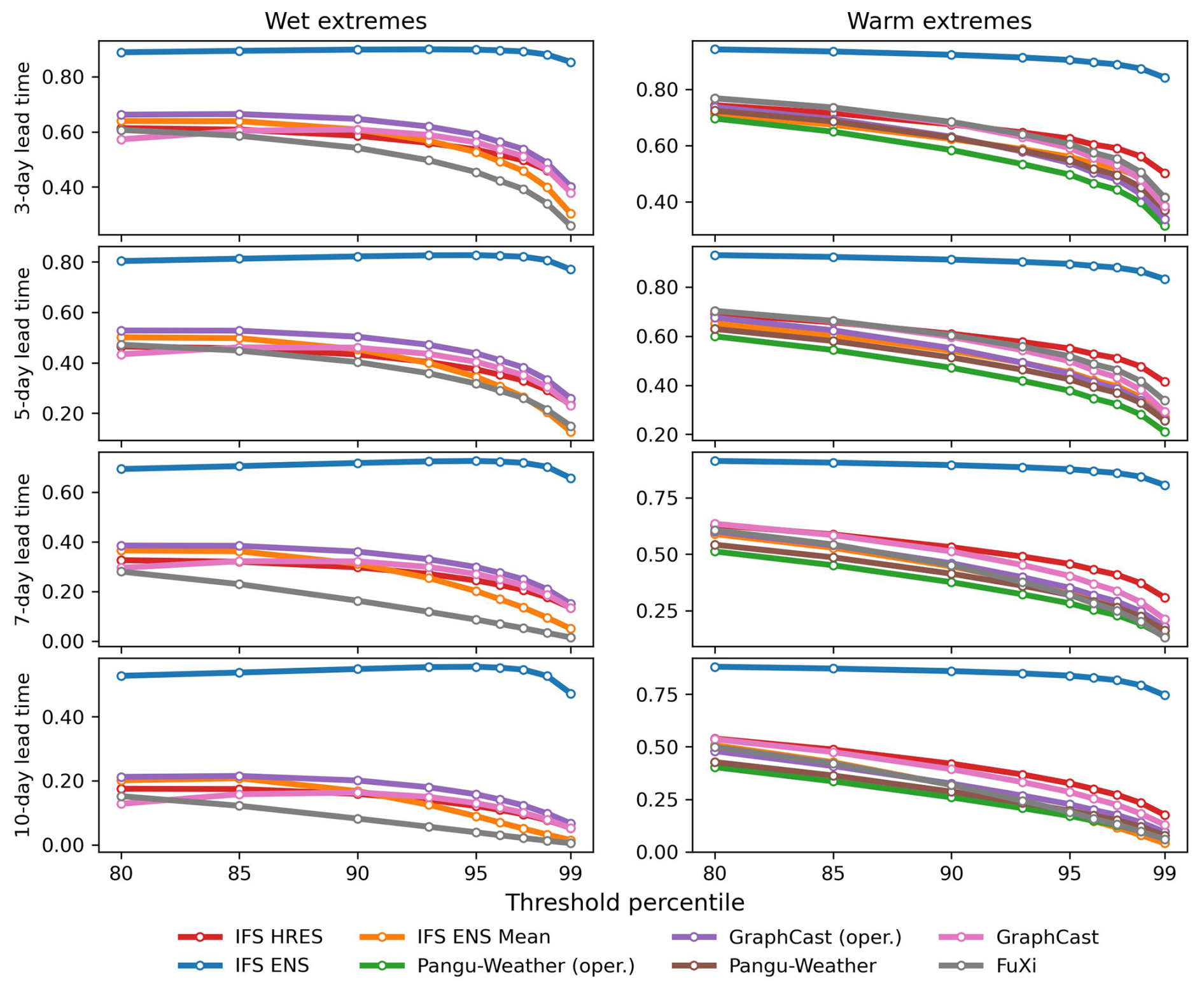
Figure 9 Globally area-weighted ROCSS for wet extremes and warm extremes with different threshold percentiles.

5 Discussion

5.1 Implications for forecaster's dilemma

Binary hydroclimatic forecasts provide useful information for disaster prevention and risk mitigation (Ben Bouallègue et al., 2024; Merz et al., 2020). Verification metrics for deterministic and ensemble forecasts of continuous variables, such as the RMSE and the CRPS, in general focus on the overall predictive performance across a range of events (Huang and Zhao, 2022; Rasp et al., 2024). They tend to reward models that minimize average errors and unrealistically smooth forecasts, leading to limited guidance when forecasting hydroclimatic extremes (Ferro and Stephenson, 2011; Rasp et al., 2020). By contrast, verification metrics of binary forecasts provide valuable additional information by emphasizing the ability to discriminate certain hydroclimatic extremes that do not directly relate to average errors (Larraondo et al., 2020). In this paper, the results show that for warm extremes, Pangu-Weather, GraphCast and FuXi tend to be more skillful than the IFS HRES within 3 d lead time but become less skillful as lead time increases. The verification of binary hydroclimatic forecasts seems to be more stringent for data-driven models since the observed lead time in which there exists outperformance of data-driven models tends to be shorter than that for continuous forecasts (Lam et al., 2023; Bi et al., 2023; Chen et al., 2023). In the Supplement, the results across global grid cells in terms of the HSS and SEDI also support this result.

The climate system is high-dimensional and complex so that there will not be a single verification metric to determine all essential characteristics of a good forecast (Rasp et al., 2024; Jolliffe and Stephenson, 2012). While verification metrics of binary forecasts emphasize discrimination, they are unable to reflect other attributes to quantify the forecast quality, such as reliability, resolution and uncertainty (Murphy, 1993). Although GraphCast is more capable of capturing the wet extremes, it tends to produce more false positives. This result implies the “forecaster's dilemma”; i.e., conditioning on outcomes is incompatible with the theoretical assumptions of established forecast evaluation methods (Lerch et al., 2017). From this perspective, a combination of multiple verification metrics and diagnostic plots is in demand (Larraondo et al., 2020; Huang and Zhao, 2022). As shown in Figs. S1 and S4 in the Supplement, the values of BS for FuXi are better than those for the HRES at a lead time of 10 d, which is different to the results for ROCSS in Fig. 4. Considering that the BS tends to reflect the average performance and is influenced by the unbalanced number of occurrences and non-occurrences, better values of a single metric do not mean more useful forecasts (Rasp et al., 2024). Overall, the process of forecast verification needs to be guided by the demand of operational applications (Ben Bouallègue and the AIFS team, 2024; Rasp et al., 2024).

5.2 Use of ground truth data

High-resolution forecasts are essential for accurately capturing multi-scale processes of hydroclimatic extremes (Liu et al., 2024a; Charlton-Perez et al., 2024; Xu et al., 2025). It is noted that hydroclimatic forecasts of coarse spatial resolution tend to miss the required small-scale variability, such as the intensity and structure of typhoons (Ben Bouallègue et al., 2024; Selz and Craig, 2023). Also, they may miss extreme values and the underlying evolution processes due to the mismatch between forecast time step and event time (Pasche et al., 2025). Therefore, there exists a demand to enhance the spatial and temporal resolution of data-driven models (Xu et al., 2024b; Zhong et al., 2024). It is noted that diffusion models have recently been shown to be effective for kilometer-scale atmospheric downscaling (Mardani et al., 2025). In addition, hybrid models that utilize global forecasts from data-driven models to drive high-resolution regional models, such as the Weather Research and Forecasting (WRF) model, can improve the forecast accuracy and resolution for extreme precipitation and tropical cyclones (Liu et al., 2024b; Xu et al., 2024b, 2025). Given that the metrics listed in Table 3 are suitable to different spatial and temporal scales, WeatherBench 2 is capable of evaluating for high-resolution forecast data.

Part of the forecast skill of data-driven models for wet extremes can stem from the unfair setting of ground truth data (Rasp et al., 2024; Lam et al., 2023). As for WeatherBench 2, it is worthwhile to note that the verification of precipitation using ERA5 reanalysis data as ground truth data is a compromised setting and should be considered as a placeholder for more accurate precipitation data (Rasp et al., 2024). While this comparison is not fair to the IFS models, the results indicate that using data-driven models to forecast global medium-range precipitation is promising. In addition, the verification is limited to the wet and warm extremes occurring in 2020 due to current data availability. The short verification period can only provide limited information about the model performance and sensitive results to the climate variability (Olivetti and Messori, 2024b). With the availability of more data on hydroclimatic forecasts and baseline ground truth observations, binary forecasts of hydroclimatic extremes deserve more in-depth verification. In the meantime, the different roles that the operational IFS analysis and ERA5 reanalysis data play in the initial conditions to generate forecasts also deserve further verification (Ben Bouallègue et al., 2024; Liu et al., 2024a; Xu et al., 2024b).

6 Conclusions

This paper presents an extension of WeatherBench 2 to binary hydroclimatic forecasts by utilizing 17 verification metrics. Specifically, the TP24h and T2M24h are calculated from the available forecasts and ground truth in WeatherBench 2, and the 90th percentiles of the ground truth data in 2020 are set as the predefined thresholds above which the wet and warm extremes are respectively detected. Through a case study of binary forecasts generated by three data-driven models and two physical models, the results show that for wet extremes, the GraphCast and its operational version tend to outperform the IFS HRES when the total precipitation of ERA5 reanalysis data is used as the ground truth. Their globally area-weighted ROCSS is 0.46, 0.50 and 0.43 at a 5 d lead time respectively. For warm extremes, GraphCast and FuXi tend to be more skillful than the IFS HRES within 3 d lead time, while they can be less skillful as the lead time increases. At lead times of 3 and 10 d, the ROCSS is 0.68 and 0.42 for the IFS HRES, 0.92 and 0.86 for IFS ENS, 0.63 and 0.29 for Pangu-Weather, 0.68 and 0.39 for GraphCast and 0.68 and 0.32 for FuXi. When the predefined thresholds of wet extremes increase from the 80th to 99th percentile, the ROCSS decreases from 0.46 to 0.24 for IFS HRES, from 0.80 to 0.77 for IFS ENS and from 0.53 to 0.26 for GraphCast (operational) at a 5 d lead time. The extension of WeatherBench 2 to binary forecasts facilitates more comprehensive comparisons of hydroclimatic forecasts and provides useful information for forecast applications.