SWAT+MODFLOW: a new hydrologic model for simulating surface-subsurface flow in managed watersheds

Coupled surface-subsurface hydrologic models are used worldwide to study historical patterns of water storage and hydrologic behaviour, investigate the impact of management strategies on water resources, and quantify the impact of changing climate, population, and policies. This study presents a new hydrologic model to simulate surface and subsurface in a physically based spatially distributed manner by linking the popular SWAT+ and MODFLOW modelling codes. Within this new code, SWAT+ simulates processes in the landscape, soils, channels, and reservoirs, whereas MODFLOW simulation groundwater processes and interaction with land surface features (soil, channels, canals, reservoirs, tile drains). Geographic connections between SWAT+ objects and MODFLOW grid cells are established a priori using a GIS and then read into the code to be used throughout the simulation to map hydrologic fluxes (recharge, soil water transfer, groundwater-channel exchange, canal seepage, tile drainage outflow, groundwater-reservoir exchange, pumping for irrigation) on a daily time step. The use and general accuracy of the model is demonstrated for two study regions that are subject to irrigation management: the Arkansas River Basin in Colorado and the San Joaquin River Basin in California. An accompanying tutorial and example model data allow for easy use of the model to other study regions. As both SWAT+ and MODFLOW are widely used worldwide for watershed and groundwater modelling, we expect that this new tool can be an important asset in many water resources projects.

1 Introduction

Watershed models are frequently used to assist with water management, water policy, and assessment of future conditions under changing climate, population, and land use. These models typically focus on land surface hydrology, streamflow, and reservoir storage and outflow. Such models include SWAT (Arnold et al., 1998) and its new version SWAT+ (Bieger et al., 2017), VIC (Liang et al., 1994), and HSPF (Duda et al., 2012). Although these models include subroutines for simulating groundwater storage, flow, and discharge to streams, they are not treated in a physically based spatially distributed manner, with groundwater flow between aquifer sections and interactions with land surface features (channels, soils, canals, etc.) not dependent on hydraulic head.

To include groundwater processes in a spatially distributed manner while preserving the use of popular modelling codes, watershed models have recently been linked to groundwater models, such as MODFLOW (Harbaugh, 2005; Niswonger et al., 2011). Several codes have been developed that link SWAT to MODFLOW, in which hydrologic fluxes from SWAT (e.g., soil recharge) are mapped to MODFLOW grid cells, and groundwater fluxes from MODFLOW (e.g., groundwater-stream exchange) are mapped to SWAT hydrologic response units (HRUs): Perkins and Sophocleous (1999), Kim et al. (2008), Guzman et al. (2015), and Bailey et al. (2016), with the latter used extensively worldwide (Wang and Chen, 2021) due to it being open source with accompanying tutorials, example datasets, and a QGIS (QGIS Development Team, 2018) user interface for linking the two models (Park et al., 2019). Example applications with the 2016 version include investigating the impact of pumping on streamflow (Molina-Navarro et al., 2019; Liu et al., 2019), assessing basin-wide water supply in managed systems (Aliyari et al., 2019; Gao et al., 2019), and quantifying the impact of climate change on water resources (Chunn et al., 2019), among many others. Other linkages include SWAT+ and MODFLOW (Bailey et al., 2020a) and GSFLOW (Markstrom et al., 2008), with the latter integrating PRMS (Precipitation-Runoff Modeling System) and MODFLOW.

With the advent of SWAT+ and its growing use worldwide, and based on the popularity of SWAT-MODFLOW, there is a need to provide a modelling code that links SWAT+ and MODFLOW for surface-subsurface hydrologic and water management applications. While Bailey et al. (2020a) provided an initial version of SWAT+MODFLOW, SWAT+ has been modified extensively in the past 5 years to include important features such as wetlands, floodplains, water allocation and water rights schemes for irrigation and municipal demand, and the use of decision tables to operate land management. In addition, the linked code did not include important features in a managed watershed, such as linking groundwater pumping to irrigation, groundwater interactions with canals and reservoirs, groundwater interaction with tile drains, and groundwater transfer to soils under conditions of a shallow water table. These features must be included for model use in highly managed river basins. In a different approach, Bailey et al. (2020b) developed a new groundwater flow module (gwflow) for SWAT+, which includes these necessary linkage features for managed areas (Yimer et al., 2023; Schulz et al., 2024). However, the model is limited to a single-layer, unconfined aquifer, and is not suite for complex geologic systems, which can be handled with MODFLOW.

In this paper, we introduce SWAT+MODFLOW, which links the newest version of SWAT+ (version 61) with MODFLOW-NWT (Niswonger et al., 2011), to create a single executable code (Fortran). Within the code, MODFLOW is called as a subroutine to simulate groundwater storage, groundwater head and flow, and groundwater interactions with soils, tile drains, channels, reservoirs, canals, and irrigated fields. A key feature for managed areas is the linkage of irrigation demand to groundwater pumping, for fields designated as receiving irrigation water from the underlying aquifer via a network of pumping wells. The model operates on a daily time step, with results output for water balance and spatio-temporal hydrologic fluxes. The new modelling code is applied to two regions as demonstration cases: the John Martin Reservoir watershed in the Arkansas River Basin, Colorado; and the San Joaquin River watershed in Central Valley, California. The models are loosely tested against historical measurements of streamflow and groundwater head. This paper is accompanied (https://zenodo.org/records/14674981, last access: 15 November 2024) by a tutorial document (SWAT+MODLFOW Tutorial.docx) that provides details of model theory and model input/output, and also the SWAT+MODFLOW compiled executable, source code, model inputs/output files for the two study regions, and video tutorials for model calibration, so that the model can be applied to other study regions.

2 Methods

This section introduces the SWAT+MODFLOW modelling code, the general method of connecting SWAT+ objects and MODFLOW grid cells, model inputs and output, and model application to two study watersheds: the John Martin Reservoir watershed (JMR; 10 056 km²) within the Arkansas River Basin, Colorado, USA; and the Middle San Joaquin-Lower Chowchilla Watershed, California (MSJ-LC; 9224 km²) within the San Joaquin River Basin, California, USA. Both regions have a semi-arid climate that requires irrigation for crop cultivation. The JMR is an irrigated semi-arid region, with irrigation provided by a network of pumping wells and irrigation canals, with the latter diverting water from the Arkansas River. Colorado water law treats surface water and groundwater as a single resource, with strict water rights governing the use of water for irrigation and domestic use. The exchange of water between surface water (Arkansas River, canals) and the aquifer is a major component of water management. The MSJ-LC is within the Central Valley of California, known for its rich agricultural history but also recent groundwater depletion (Ojha et al., 2018; Vasco et al., 2019; Jasechko and Perrone, 2020; Liu et al., 2022) due to excess pumping for irrigation. Modelling theory is presented within the context of the two study regions to facilitate understanding of modelling details.

2.1 SWAT+ theory and models

The Soil and Water Assessment Tool (SWAT; Arnold et al., 1998) is a widely used hydrologic model for simulating hydrologic processes and water resources in watershed systems (e.g., Liu et al., 2021; Cao et al., 2023; Tefera et al., 2023). SWAT is a quasi-distributed, continuous-in-time, process based, basin-scale model that simulates hydrologic processes at a higher spatial resolution by classifying the watershed into hydrologic response units (HRUs). HRUs are computational units, each with distinct land use, soil, and slope composition (Neitsch et al., 2011) within a given subbasin.

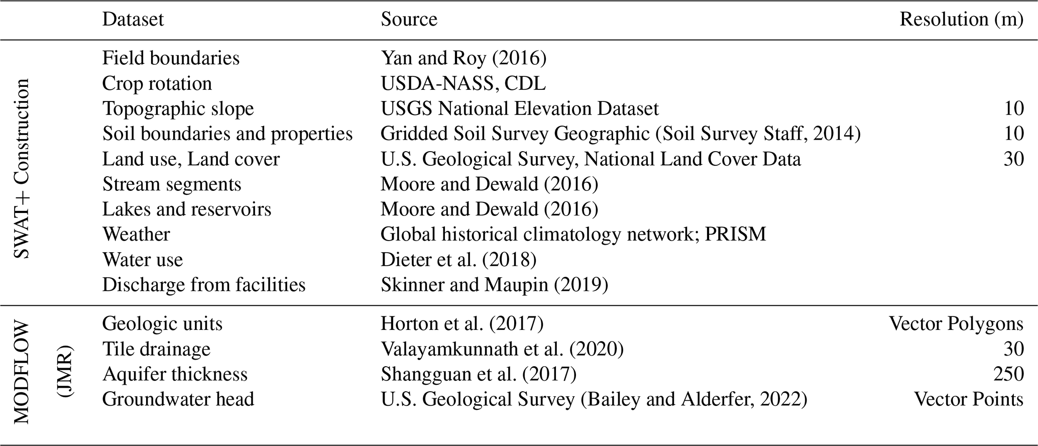
The SWAT+ model (Bieger et al., 2017), the upgraded version of SWAT, offers improved hydrologic connections within a watershed system. The base SWAT+ model has the capability to simulate the movement of sediment, water, and nutrients via a network of connected hydrologic objects (HRUs, landscape units, aquifers, ponds, wetlands, reservoirs, channels) in the watershed's landscape. Users determine the path by which water, nutrients, and sediment are directed from one entity to another. The watershed is partitioned into routing units (i.e., subbasins), which aggregate hydrographs and sediment/nutrient mass from different HRUs and facilitate their transport over the landscape and through the network of channels. The basic SWAT+ objects for the two study regions are presented in Fig. 1 and Table 1. JMR has 101 subbasins, 1324 channels, and 10 611 HRUs, of which 5101 are assigned to boundaries of individual, cultivated fields. MSJ-LC has 87 subbasins, 2763 channels, and 18 821 HRUs, of which 13 349 are cultivated. The data sources for the delineation of these objects are listed in Table 2.

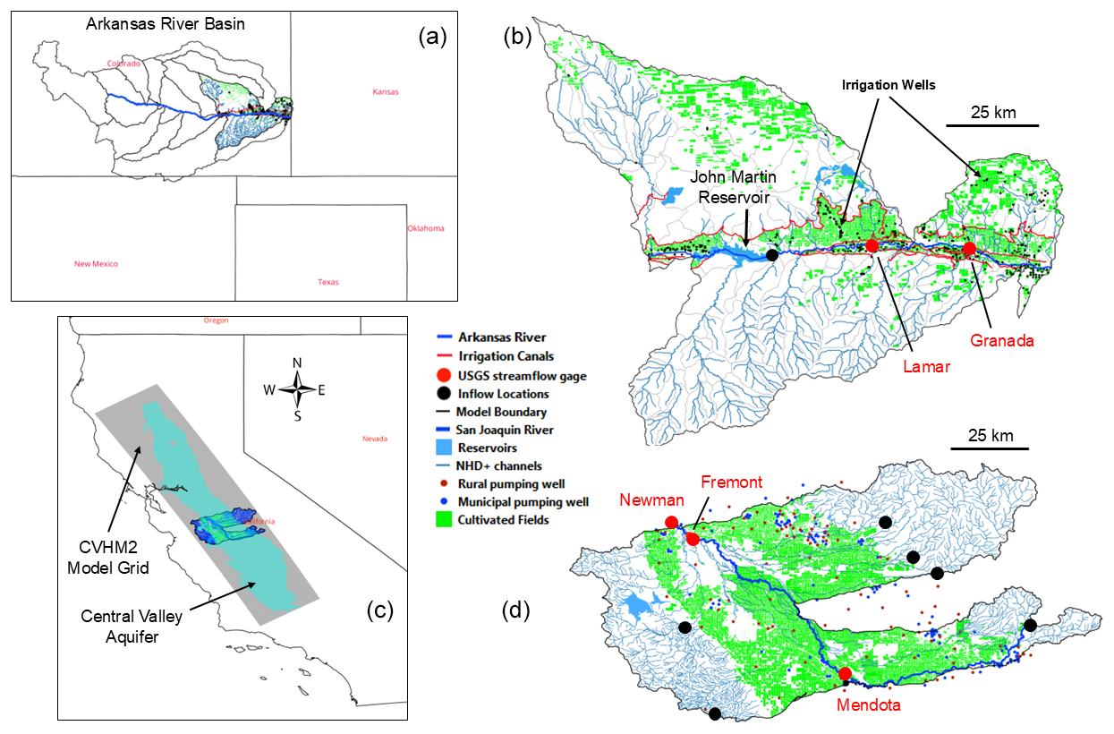
Figure 1 Maps of the two study regions: (a) and (b) show the location and hydro-management details of the John Martin Reservoir Watershed, Colorado (HUC8 11020009); (c) and (d) show the location and hydro-management details of the Middle San Joaquin-Lower Chowchilla Watershed, California (HUC8 18040001). Panel (c) shows the spatial extent of the Central Valley aquifer and the CVHM2 MODFLOW model. Stream gages are shown on both study region maps. NHD+ channels = stream segments from the digital stream network of the United States (Moore and Dewald, 2016). For the John Martin Reservoir model, the aquifer extent is the same as the watershed boundary.

Table 1 Watershed features and modelling objects of the two study regions. HUC8 = 8-digit watershed identifier, for watershed subbasins within the United States.

Table 2 Datasets used in the construction of the original SWAT+ models and the gwflow inputs.

SWAT+ operates on a daily time step. For each day of the simulation, a water balance is performed for the soil profile of each HRU; for each channel segment of the channel network; for each aquifer unit of the aquifer system; and for each pond, lake, and reservoir. Water balance calculations yield daily fluxes (m³ d⁻¹) and updated storage volumes (m³) for soil water, channel water, groundwater, and reservoir water. Contributions to the channel network, which makes up the water yield of a watershed, include surface runoff from HRUs; soil lateral flow from HRUs; tile drainage outflow from HRUs; groundwater discharge from aquifer units; and point sources or diversions, for example from wastewater treatment plants (WWTPs) or to irrigation canals. For the JMR model, the measured outflow (USGS station 07130500; Arkansas River below John Martin Reservoir, CO) from John Martin Reservoir (see Fig. 1b) is used as a point source to specify daily inflow to the SWAT+ channel representing the reach of the Arkansas River. For the MSJ-LC model, measured monthly outflows in the hill areas surrounding the valley are used as point sources to specify monthly inflow to corresponding SWAT+ channels (data accessed from https://www.sciencebase.gov/catalog/item/61e7442ed34e3618e01cf68f, last access: October 2024). For both models, canal diversions are included as negative point sources at diversion points along the Arkansas River and San Joaquin River. In this study, when SWAT+ is linked with MODFLOW, the original aquifer module of SWAT+ is deactivated.

2.2 MODFLOW theory and models

MODFLOW is a Fortran-based computer program that simulates the storage, head, and movement of groundwater in a multi-dimensional aquifer system in a physically based spatially distributed manner. To solve for groundwater storage, head, and flow in a spatially distributed manner, the aquifer is discretized into a grid of rows and columns, making up a network of connected grid cells. A groundwater balance is applied to each cell, accounting for groundwater inflows (e.g., recharge, injection, canal seepage, lake seepage, channel seepage), groundwater outflows (e.g., pumping, evapotranspiration, groundwater discharge to channels, tile drainage outflow), and the resulting change in storage, for either unconfined or confined conditions. The model uses Darcy's Law to simulate groundwater flow between neighbouring cells, and a set of input files to specify inflows, outflows, initial head conditions, and boundary conditions for designated cells within the model domain. Key aquifer properties that govern groundwater flow and storage include hydraulic conductivity (K) (vertical, horizontal), specific yield (S_y) (for unconfined aquifers), and specific storage (S_s) (for confined aquifers). For interaction with surface or near-surface features such as channels, lakes, and tile drains, additional required input parameters include feature elevation (e.g., channel bed elevation, channel stage), channel/lake bed conductance, and drainage material conductance. Inflow and outflow features are included in the model using packages, with a separate input file for each package. Typical packages include Recharge, River, Lake, Drain, Well, Reservoir, and ET. A full list of packages and associated instructions to create input files is available at: https://water.usgs.gov/ogw/modflow-nwt/MODFLOW-NWT-Guide/index.html (last access: November 2024). Models typically are applied to the saturated zone of aquifers. However, with the use of the Unsaturated-Zone Package (UZF; Niswonger et al., 2006), flow in the unsaturated zone can also be simulated.

Several MODFLOW versions are available: MODFLOW-2005 (Harbaugh, 2005), MODFLOW-NWT (Niswonger et al., 2011), and MODFLOW 6 (Langevin et al., 2017). For this study, we link SWAT+ to MODFLOW-NWT, as was done previously for SWAT-MODFLOW (Bailey et al., 2016). A MODFLOW-NWT model was therefore constructed for the two study regions. For both regions, we used 500 m grid cells, resulting in 311 rows and 280 columns for JMR and 189 rows and 336 columns for MSJ-LC. For the JMR, the aquifer boundary is the same as the watershed boundary (see Fig. 1b), resulting in 41 542 active cells. For the MSJ-LC, only the 33 012 cells within the delineation of the Central Valley aquifer (see Fig. 1c for the aquifer boundary) are active. Both models use a single layer to represent the unconfined aquifer. Deeper confined layers are not included in the models.

The datasets used to construct the MODFLOW model for the JMR are listed in Table 2, with ground surface elevation (m above sea level) and geologic units shown in Fig. 2a, b. Each grid cell is assigned a ground surface elevation and bottom elevation, using the dataset of unconfined aquifer thickness (Table 2); an initial value of hydraulic conductivity (K) and specific yield (S_y) using the map of geologic units; an elevation and conductance for tile drains if a tile drain is present; and an initial value of groundwater head (m), based on a spatial interpolation of measured groundwater head (m) from a network of 10 USGS monitoring wells for the year 2000.

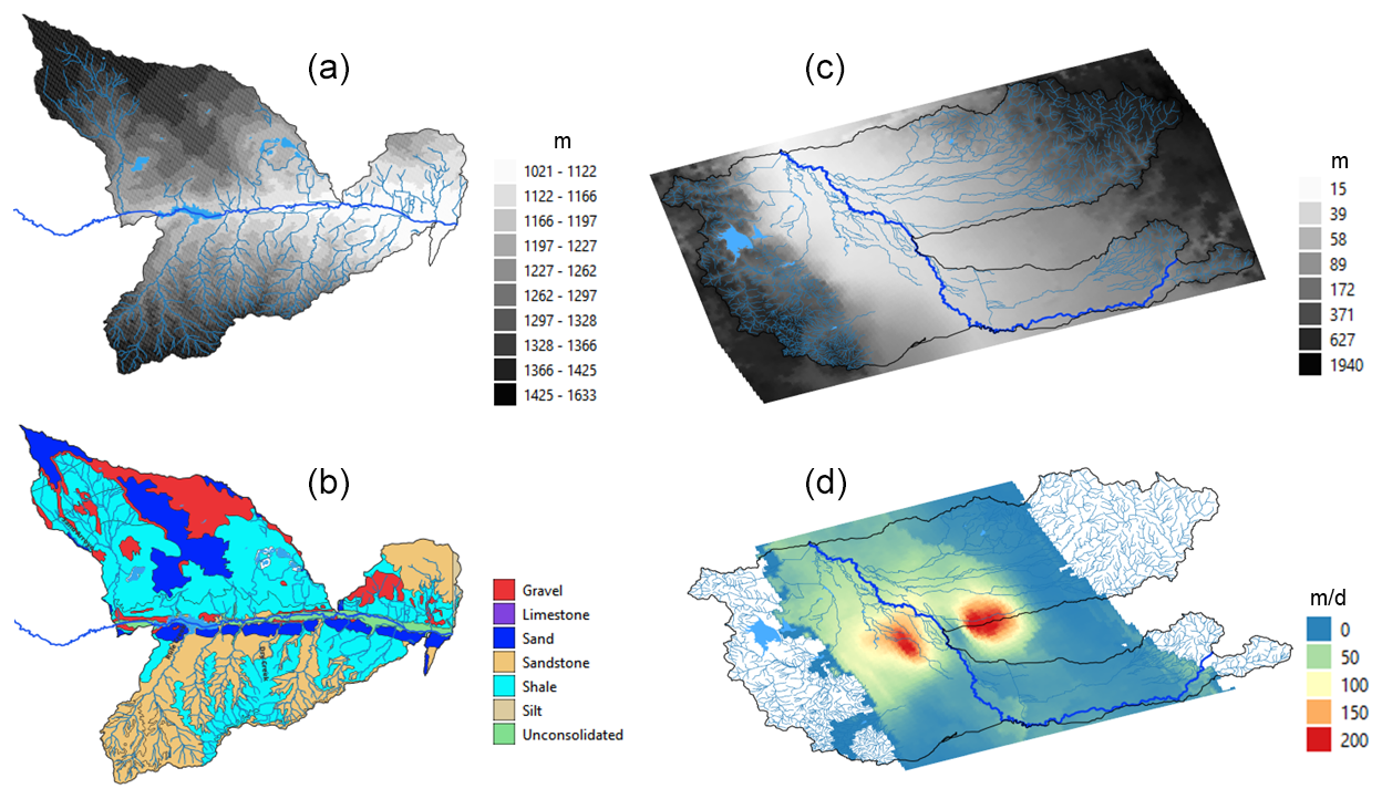
Figure 2 Maps of the two study regions showing MODFLOW details: (a) and (b) show the ground surface elevation (m a.s.l., meter above sea level) and geologic unit for John Martin Reservoir Watershed, and (c) and (d) show the ground surface elevation (masl) and horizontal hydraulic conductivity (m d⁻¹) of the unconfined aquifer.

The data for population grid cell properties for the MSJ-LC model are extracted from the Central Valley Hydrologic Model version 2 (CVHM2) (Faunt et al., 2024; model data available at https://www.sciencebase.gov/catalog/item/65bd367fd34e18c6baf32758, last access: July 2024), a MODFLOW model which spans the entire Central Valley aquifer region (see Fig. 1c for delineation of the Central Valley aquifer and the CVHM2 grid). The CVHM2 model is constructed using 1 mile grid cells (1609.3 m) for a total of 441 rows and 98 columns and runs for 702 monthly stress periods spanning April 1961 to December 2019. The model uses 13 layers to discretize the vertical extent of the aquifer. Data used to populate model input include climate (precipitation, ET, runoff from surrounding hills), pumping (agricultural, rural, municipal), monthly measured inflows and river diversions, and well lithology for aquifer properties. For the MSJ-LC model used in this study, a geographic connection (intersection) was created between the CVHM2 grid cells (1609.3 m) and the MSJ-LC grid cells (500 m), using GIS shape files of both grids. Using these connections, cell values from the larger model (CVHM2) were mapped to the smaller “daughter” model. Variables for mapping include time-varying boundary conditions (CHD package), elevations (DIS package; see Fig. 2c for top elevation), aquifer properties (UPW package), municipal and rural pumping (WELL package; re-written from the MNW2 package used in CVHM2), and initial groundwater head (m). Agricultural pumping is simulated using the water allocation module of SWAT+, as explained in Sect. 2.3.5. Due to the smaller model using only a single layer, aquifer properties were averaged (weighted average for horizontal K by layer thickness, see Fig. 2d; harmonic average for vertical K; weighted average for S_s) over the 13 original layers. Figure 2d shows K values whereas Fig. 2b shows geologic unit boundaries, as the aquifer properties for the JMR model have not yet been calibrated. Boundary cells were identified from the spatial extent of the Central Valley aquifer within the MSJ-LC boundary, with monthly values of groundwater head extracted from the CVHM2 model simulation.

2.3 Linking SWAT+ and MODFLOW

2.3.1 Model overview

SWAT+MODFLOW was developed in this study as a single Fortran code that integrates the MODFLOW-NWT code into the SWAT+ code (version 61.0; https://swat.tamu.edu/software/plus/, last access: March 2024). During the SWAT+ simulation, MODFLOW is called as a subroutine to simulate groundwater storage, groundwater head, and interaction with SWAT+ hydrologic objects such as soils, channels, and reservoirs. All calculations for SWAT+ and MODFLOW and variable interactions occur on a daily time step. We have written 13 new subroutines into the SWAT+ code to run MODFLOW, map variables between SWAT+ objects and MODFLOW grid cells, and write results to output files. Figure 3 shows a diagram summarizing the hydrologic fluxes simulated by SWAT+ (blue text) and MODFLOW (yellow text) within the SWAT+MODFLOW code. Within the code, the subroutines used to link SWAT+ and MODFLOW are given the prefix “smrt” (swat-modflow-rt3d). Although this paper does not report results of nutrient (nitrogen, phosphorus) transport in groundwater using RT3D (Wei et al., 2019; Wei and Bailey, 2021), the current code contains this functionality and will be reported in a follow-on study. The linkage input files and output files specific to MODFLOW also are given the prefix “smrt”. The groundwater fluxes, the corresponding SWAT+ objects to which they are linked, the corresponding MODFLOW package that simulates the flux, the input file that contains the linkage information, and the flux abbreviation used in inputs and outputs, are listed in Table 3. Temporal watershed-wide groundwater fluxes (mm; normalized by watershed area) are output on a daily, monthly, annual, and average annual basis, using a set of output files. Spatial (cell-by-cell) flux values (m³ d⁻¹) are written to output files for each month and year, for each groundwater flux. The next sections provide details for each of the 7 fluxes listed in Table 3. More details and file explanations are provided in Supplement.

Figure 3 Cross-section of watershed, showing fluxes simulated by SWAT+ and MODFLOW.

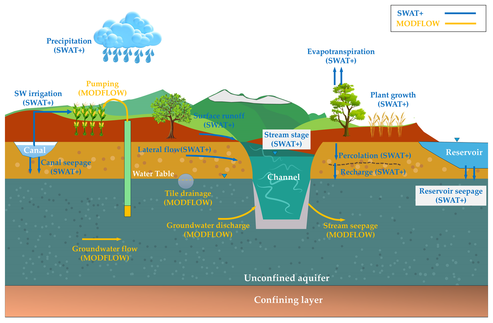
Table 3 Summary of SWAT+ connections, MODFLOW package, and input/output for each simulated groundwater flux in SWAT+MODFLOW.

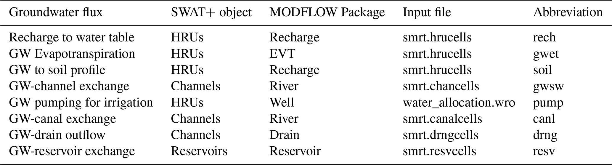
2.3.2 Recharge (soil to aquifer) and soil transfer (aquifer to soil)

Water can be exchanged between the soil profile and the unconfined aquifer in two directions: from the soil profile to the aquifer, if the water table is at or below the base of the soil profile (Fig. 4a), and from the aquifer to the soil profile, if the water table is within any layer of the soil profile (Fig. 4b).

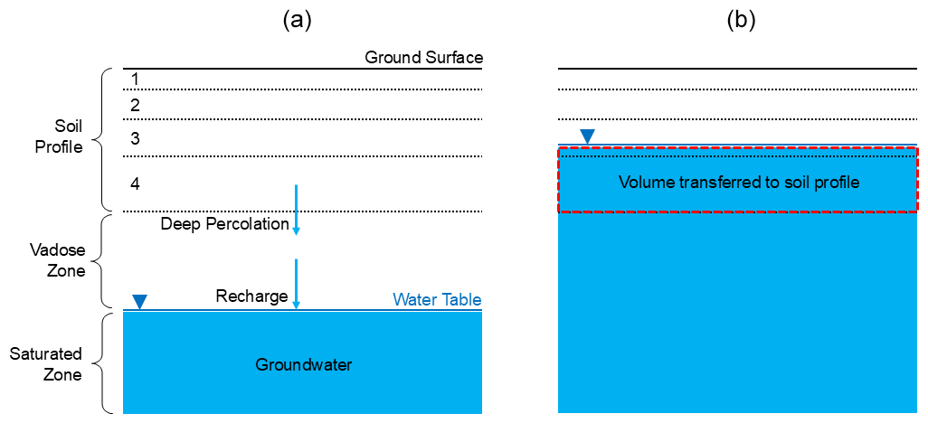
Figure 4 Schematics showing process of deep percolation and recharge for the condition of (a) water table disconnected from the soil profile and (b) water table within the soil profile.

In the first scenario, recharge to the water table originates from deep percolation that exits the bottom of the soil profile. Deep percolation and recharge are first calculated for each HRU (on a daily time step) and then transferred to the MODFLOW grid cells for the Recharge package. Routing through the vadose zone is not simulated in a physically based manner, but rather using a transfer function:

$$\begin{array}{}\text{(1)}& R_i=\left[\left(\mathrm{1}-e^{-\mathrm{1}/\mathit{\delta }}\right)\cdot {\mathrm{dp}}_i\right]+\left[e^{-\mathrm{1}/\mathit{\delta }}{R}_{i-\mathrm{1}}\right]\end{array}$$

where dp_i is the depth (mm) of deep percolation for the current day i, R is the recharge from the previous day (i−1) and the current day i, and δ is the recharge delay term (days). The term on the left is the recharge from the current day's deep percolation, and the term on the right is the recharge from the previous day's deep percolation. The transfer function spreads out the recharge temporally, so that portions of the deep percolation water reach the water table at different times. Once daily recharge is calculated for each HRU, the amount of recharge (m³ d⁻¹) to each individual MODFLOW cell is calculated by summing the contribution from all intersecting HRUs:

$$\begin{array}{}\text{(2)}& R_{\mathrm{cell}}=\sum _{i=\mathrm{1}}^n{V}_{{\mathrm{hru}}_i}{F}_{{\mathrm{hru}}_i}\end{array}$$

where V_hru is the daily volumetric flow rate of recharge (m³ d⁻¹) for the ith HRU connected to the grid cell, and F_hru is the fraction of the ith HRU that is occupied by the cell. For example, Fig. 5a shows the geographic intersection between cell 49 174 and 3 HRUs, highlighted in yellow (6908, 7011, 7012), for the JMR model. The area of each HRU is 412 200, 85 500, and 234 900 m², respectively. The overlapping area between the cell and each HRU is 134 080, 39 275, and 31 211 m², respectively, resulting in HRU fractions of 0.325, 0.460, and 0.133, respectively.

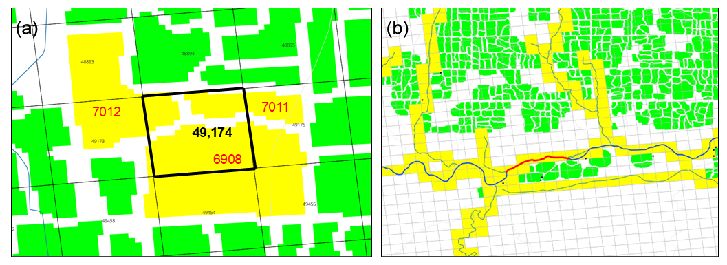
Figure 5 Maps showing spatial connections between (a) HRUs and grid cells and (b) channels and grid cells.

In the second scenario, in which the water table rises to within the soil profile, the groundwater volume within the soil profile is removed from the grid cell and transferred to the HRU soil profile, which then is subject to soil water processes such as plant transpiration, soil evaporation, soil lateral flow, tile drainage, saturation excess flow, or recharge to the water table. The volume of groundwater V_gw transferred to the soil profile is:

$$\begin{array}{}\text{(3)}& V_{\mathrm{gw}}=d_{\mathrm{sat}}\cdot F_{\mathrm{cell}}\cdot S_{\mathrm{y}}\end{array}$$

where d_sat is the depth of soil profile saturated by the water table (m) (i.e., the vertical distance from the water table to the base of the soil profile), F_cell is the area of the cell the resides spatially in the HRU (m²), and S_y is the aquifer specific yield. This volume is then added to the soil storage array of the soil layers, based on the fraction of the layer that is saturated.

2.3.3 Groundwater ET

ET from the saturated zone is simulated using the EVT package of MODFLOW. Groundwater ET is calculated only if the water table in a grid cell is above a specified elevation z_bot (m), calculated by subtracting a specified ET extinction depth EXDP (m) (i.e. the depth below which ET cannot occur) from the ground surface z_surf. The maximum depth of ET that can be removed from the saturated zone is equal to the unsatisfied ET, referred to as ET_remain (mm), set equal to the difference between the potential ET (mm) and the actual ET (mm) simulated for each HRU soil profile for the day. The connection between HRUs and grid cells for mapping unsatisfied ET is the same as for mapping soil percolation to grid cell recharge. The depth of groundwater ET (mm) removed from the cell is calculated using the following linear relationship:

$$\begin{array}{}\text{(4)}& \begin{array}{l}{h}_{i,j}<z_{\mathrm{bot}}\to {\mathrm{ET}}_{\mathrm{GW}}=\mathrm{0}\\ h_{i,j}>z_{\mathrm{bot}}\to {\mathrm{ET}}_{\mathrm{GW}}={\mathrm{ET}}_{\mathrm{remain}}\cdot \left(\frac{h_{i,j}-z_{\mathrm{bot}}}{z_{\mathrm{surf}}-z_{\mathrm{bot}}}\right)\end{array}\end{array}$$

The depth of groundwater ET is multiplied by the horizontal spatial area of the HRU to provide a volumetric flow rate in m³ d⁻¹, and then divided amongst the cells connected to the HRU. This groundwater volume is removed from the grid cell. Simulating groundwater ET occurs if the EVT package of MODFLOW is activated.

2.3.4 Groundwater-channel exchange

Exchange of water between the aquifer and stream channels is simulated using the River package of MODFLOW. Within the River package, Darcy's Law is used to calculate the daily volumetric flow rate Q (m³ d⁻¹) of exchange by comparing the groundwater head (h_gw) in the grid cell to the stream stage (h_stream) in the channel. If the groundwater head is higher than the stream stage, then groundwater discharges through the channel bed into the channel. If, however, the groundwater head is lower than the stream stage, then stream water seeps through the channel bed into the aquifer. For these calculations, channel width (m) and simulated daily channel stage (m) are provided by SWAT+ channel routines; channel bed conductivity (m d⁻¹), channel bed elevation (m), and channel bed thickness (m) are provided in MODFLOW inputs; groundwater head (m) in the cell is simulated on a daily basis; and the channel length (m) within each grid cell is provided by a geographic intersection between SWAT+ channels and intersecting MODFLOW grid cells (Fig. 5b; yellow cells are in connection with SWAT+ channels). The channel highlighted in red (channel #497) is along the Arkansas River and is in connection with 7 grid cells. Through an intersection routine within GIS, the length L of the channel within each of the grid cells is 428, 532, 562, 513, 131, 525, and 119 m. The length of the channel within the grid cell is directly proportional to the area of channel bed in connection with the aquifer and therefore is a strong control on the amount of water that can be transferred between the aquifer and the channel. If SWAT+ is linked with MODFLOW, then the regular channel seepage calculation with the channel control subroutine is not used. Therefore, the hydraulic conductivity of channel bed sediments as listed in the SWAT+ input files is not used.

2.3.5 Groundwater pumping for irrigation demand

For a standard SWAT+ model, the water allocation module can be used to control water transfer between SWAT+ objects for water demand conditions, such as irrigation. Sources of irrigation water can include channels, reservoirs, aquifers, or unlimited (i.e., water sourced from outside the model domain). For the JMR model, HRUs receive irrigation water from channels (via canal diversions), groundwater, and unlimited (canals that divert water upstream of the watershed boundary, for the Fort Lyon canal). For the MSJ-LC model, HRUs receive irrigation water from channels and groundwater. For SWAT+MODFLOW, if the irrigation source in the water allocation input is specified to be “aquifer”, then MODFLOW simulates groundwater pumping to satisfy the irrigation demand. Irrigation will occur only if sufficient groundwater is available in the grid cell. If the irrigation demand is greater than the available groundwater in the cell, then all groundwater is removed to satisfy a portion of the demand. Pumping can occur either (1) in a single cell, or (2) from all grid cells connected geographically to the demand HRU. This option is controlled in the water allocation input file.

The details of the simulation of irrigation demand and irrigation supply is shown in Fig. 6. Crop growth is simulated on a daily basis given daily weather, crop type, and management operations. When soil water stress, defined as the fraction of potential plant growth achieved due to soil water deficit, reaches a threshold value (specified by the user), an irrigation demand is triggered for the target HRU. Irrigation is then withdrawn from the specified source (channel, reservoir, aquifer, unlimited), conditional to the available water volume in the source object. Multiple irrigation sources can be specified for each demand object, with the order and demand fraction specified for each source. A specified depth (mm) of water is then applied to the field, and then subject to a runoff ratio. For both models, the applied irrigation depth is set to 25.4 mm (1 in.) and the soil water stress is set to 0.80.

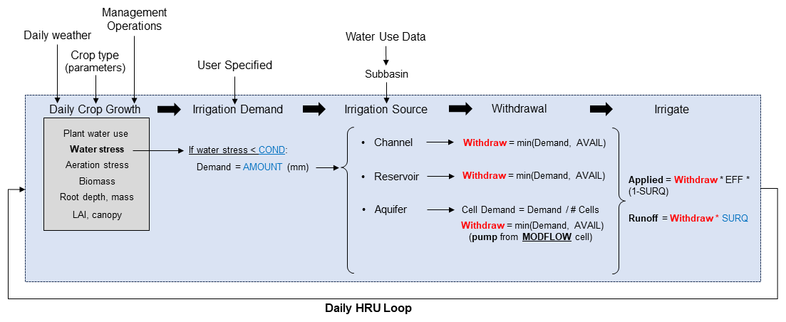
Figure 6 Flow process within the SWAT+ code to simulate demand-driven irrigation events, for each field HRU on a daily basis. Irrigation events are triggered by a specified water stress (COND) in the soil profile. This irrigation demand (depth of water AMOUNT ⋅ area of field = m³) is then compared to available water storage AVAIL in the source object (channel, reservoir, or aquifer) to determine the volume Withdraw (m³ d⁻¹) that can be removed from the object and applied to the field as irrigation. For the aquifer, the demand is compared to groundwater stored in the MODFLOW cell that underlies the field, to determine how much can be pumped. Finally, the irrigation water is applied to the HRU, and runoff is calculated using the runoff ratio SURQ.

2.3.6 Groundwater-canal exchange

Earthen irrigation canals often seep water to the underlying unconfined aquifer. They can also receive groundwater if the water table is higher than the canal stage. In SWAT+MODFLOW, this exchange is simulated using MODFLOW's River package. The exchange rate (m³ d⁻¹) is calculated using Darcy's Law, for each MODFLOW grid cell in geographic connection with an irrigation canal:

$$\begin{array}{}\text{(5)}& Q_{\mathrm{canl}}=A_{\mathrm{bed}}{K}_{\mathrm{bed}}\left({\displaystyle \frac{h_{\mathrm{canl}}-h_{\mathrm{gw}}}{d_{\mathrm{bed}}}}\right)\end{array}$$

where A_bed = the area of the canal bed in contact with the aquifer within the grid cell (m²) = the width of the canal (m) ⋅ the length of the canal in the grid cell (m); K_bed = the hydraulic conductivity of the canal bed material (m d⁻¹); h_canl = the head (stage) of the canal water (m); h_gw = the head of groundwater in the grid cell (m); and d_bed = the thickness of the canal bed material (m).

Canal seepage is simulated for the JMR model. For the JMR model, there are 17 canals (see Fig. 1b). When intersected with the MODFLOW grid, there are 1277 grid cells that are designated as “canal cells” (Fig. 7a), and for which the exchange rate is calculated. The length of the canal in the grid cell is determined from the intersection results. The exchange rate should be calculated only when there is water in the irrigation canal. For the JMR model, this is between 1 April and 15 October of each year. If the irrigation canal is connected to a point source diversion, such as with the JMR model, then calculated canal seepage is provided by the water already diverted to the canal from the channel source. Therefore, diverted canal water can provide both irrigation water to fields and canal seepage to the underlying aquifer. If groundwater discharges to the canal (i.e., groundwater head > canal stage within the grid cell), then this volume is added to the water diverted into the canal, which can be used for irrigation in downstream areas within the canal command area.

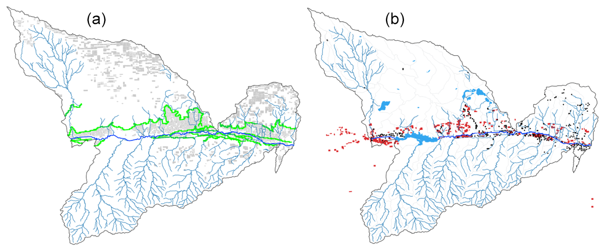
Figure 7 (a) Canal cells (green) and (b) tile drain cells (red) for the JMR model. In (a), the gray polygons indicate boundaries of cultivated fields.

2.3.7 Groundwater-drain exchange

Subsurface drains (“tiles”) are often placed in agricultural landscapes to drain excess soil water and groundwater. SWAT+ has a tile drainage routine. While this routine removes excess soil water, drainage should also occur if groundwater rises to the level of the drains. This can be simulated in SWAT+MODFLOW using MODFLOW's drain package. Within the package, groundwater head (m) is compared to the drain elevation (m); if the head is higher than the drain, then groundwater is removed via the drain. With new SWAT+MODFLOW linkage routines, this removed groundwater is transferred to specified SWAT+ channels for channel routing. The groundwater-drain feature for SWAT+MODFLOW is activated using the Drain package of MODFLOW. For the JMR model, there are 814 Drain cells (Fig. 7b), as identified by the national dataset of Valayamkunnath et al. (2020). The channel to which drainage water is transferred was determined by proximity to the Drain cell.

2.3.8 Groundwater-reservoir exchange

Water can be exchanged between reservoirs and an underlying unconfined aquifer. Within SWAT+MODFLOW, this exchange can occur between reservoirs objects and MODFLOW grid cells, using MODFLOW's Reservoir package. The reservoir package uses Darcy's Law to calculate the transfer of water from the aquifer to the reservoir, or from the reservoir to the aquifer, depending on their relative position. For each daily time step of the simulation, the reservoir stage is updated using the simulated reservoir depth of the reservoir object. If MODFLOW is active, then the original seepage calculation in the reservoir control subroutine is not used. In the JMR model there are 302 MODFLOW grid cells that are connected to reservoir objects. For each cell, the connected reservoir object, stage (m), depth (m), hydraulic conductivity (m d⁻¹), and bed thickness (m) are listed are specified.

2.4 Summary of code, inputs, and outputs

The model inputs, model code structure, and model outputs are summarized in Fig. 8. Model inputs consist of SWAT+ inputs, MODFLOW package inputs, and smrt inputs, with the latter containing all necessary geographic connectivity (HRUs, channels, canals, reservoirs, drains) between SWAT+ objects and MODFLOW cells. Within the code structure diagram, blue text indicates new subroutines for SWAT+MODFLOW. “smrt_initialize” reads in all object connections. For each daily time step, “smrt_well” is called to determine pumping rates for MODFLOW cells, if groundwater irrigation is specified for HRUs. During the “command” subroutine, HRU (“hru_control”) and routing unit (“ru_control”) calculations are first performed, followed by “smrt_run”, which maps SWAT+ variables (recharge, unsatisfied ET, channel stage, canal stage, reservoir stage) to MODFLOW cells, runs MODFLOW, and then maps MODFLOW variables (channel exchange, canal exchange, drain exchange, reservoir exchange) to SWAT+ objects. Reservoir calculations (“res_control”), point sources (“recall”), and channel routing (“sd_channel_ control”) are then called to complete the daily time step. The subroutine “smrt_output” is then called to compute and output watershed-wide groundwater fluxes (mm) and cell-by-cell fluxes (m³ d⁻¹) to output files.

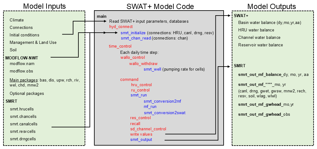
Figure 8 Diagram showing the model inputs, basic model code structure, and model outputs for SWAT+MODFLOW. MODFLOW packages: bas = basic, dis = discretization, upw = upstream weighting (aquifer properties), rch = recharge, riv = river, wel = well, chd = constant head boundary, mnw2 = multi-node pumping. SWAT+ code: smrt = swat-modflow-rt3d; wallo = water allocation routine; hru = hydrologic response unit; ru = routing unit; res = reservoir; recall = point source.

2.5 Model simulations for the two study regions

The JMR model is run for the 2000–2008 period. As an example of performing global sensitivity analysis, the JMR is run with PEST$++$ (White et al., 2020; object-oriented code written in C$++$ that extends the algorithms of the original PEST program) for the Morris Method. Details, a parameter list, and results are provided in the accompanying tutorial (Supplement). In the Morris Method (Morris, 1991), the influence of a selected model parameter is assessed by quantifying the ratio of the change in the simulated response (e.g., streamflow, groundwater head) to the change in parameter value. This ratio is calculated for multiple base values of the parameter, with the collection of ratios then averaged to provide an overall sensitivity index for the parameter. This process is repeated for all selected model parameters, with the parameters then ranked according to their sensitivity index. Parameters with the highest index have the highest control on model output.

Stream channel Manning's roughness, aquifer hydraulic conductivity, specific yield, channel bed conductivity, and channel bed thickness control streamflow in the downstream portion of the Arkansas River. As an example of performing model calibration for a SWAT+MODFLOW, the JMR model is also calibrated using PEST (Doherty, 2020) for monthly streamflow at the two USGS streamflow gages (Lamar, Granada) and annual groundwater head (m) at the 10 USGS monitoring wells. PEST files and results are provided as Supplement. The MSJ-LC model is run for the 1981–2019 period. This model is not calibrated, with model results deemed sufficient for the purpose of presenting the SWAT+MODFLOW code. The Nash-Sutcliff Efficiency (NSE) factor is used to assess model performance for streamflow generation. Both models are analysed for water balance and spatio-temporal land surface, channel, and groundwater fluxes.

Model simulations are run on a desk-top computer, 13th Gen Intel(R) Core(TM) i7-13700 2.10 GHz; with 64 GB installed RAM. Model run-times for the JMR and MSJ-LC models are 25 and 112 min, respectively, resulting in ∼ 3 min per simulation year. If SWAT+ is run with MODFLOW, run-times are 7 and 58 min, respectively, or ∼ 0.8 and 1.5 min per simulation year. Therefore, including MODFLOW for these two regions increases model run-time by 250 % and 100 %, respectively. These increases seem to be acceptable for model applications such as calibration, sensitivity analysis, and uncertainty analysis which often require hundreds or thousands of model runs.

3 Results and discussion

General model output is presented here to demonstrate the correctness of the SWAT+MODFLOW code, in terms of water balance, streamflow generation, and groundwater storage and fluxes. As these models are not intended for use in scenario analysis, a comprehensive model calibration has not been attempted.

3.1 General water balance

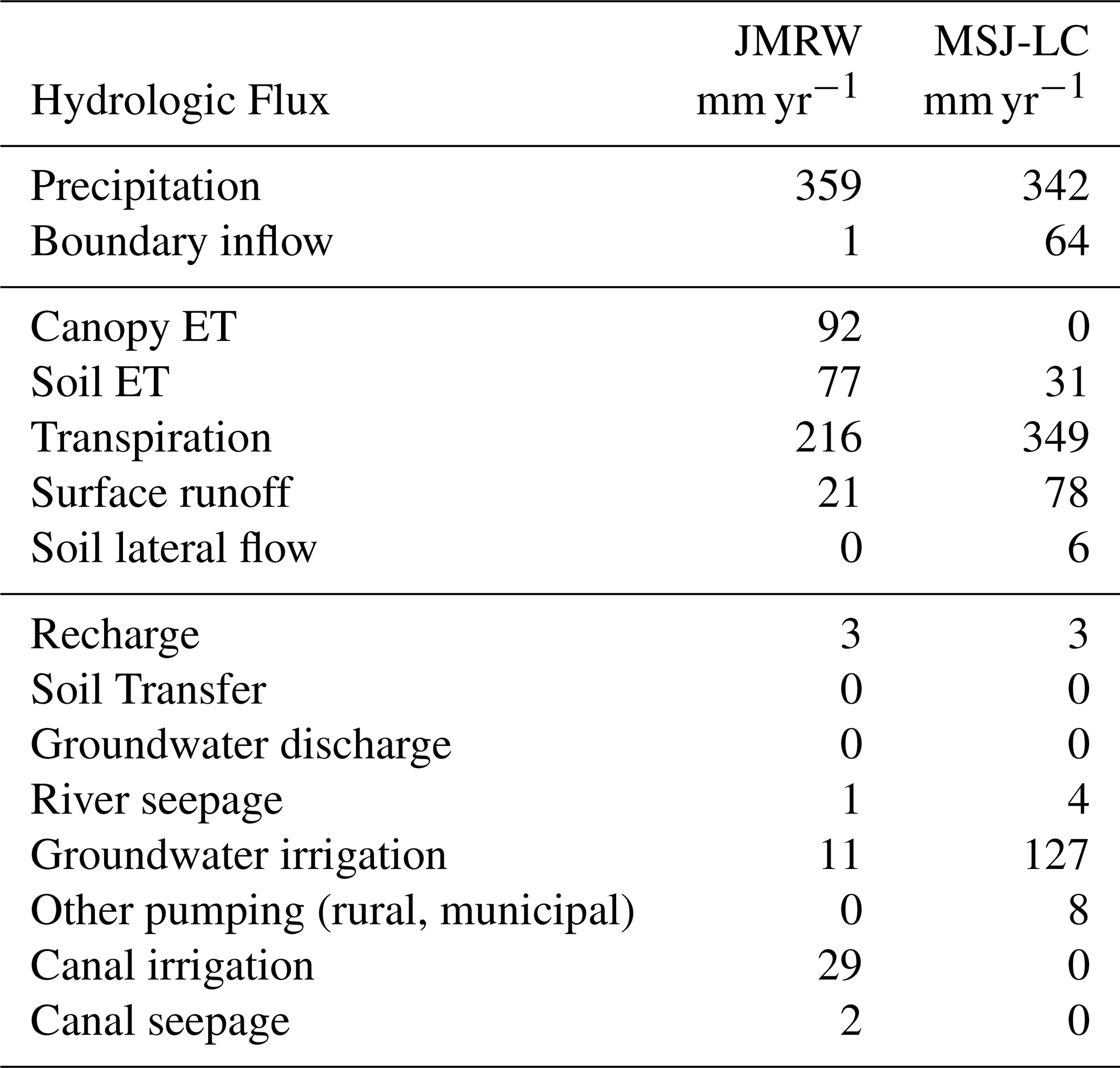
Average annual hydrologic fluxes for the two study regions are presented in Table 4. Both regions are semi-arid, with annual precipitation of only 359 and 342 mm yr⁻¹ for JMR and MSJ-LC, respectively. Due to extensive groundwater pumping in the MSJ-LC (127 mm yr⁻¹ for irrigation as compared to 11 mm yr⁻¹ for JMR; 8 mm yr⁻¹ for rural and municipal pumping), significant groundwater inflow along the model boundary (64 mm yr⁻¹) occurs. Surface runoff fraction (surface runoff/precipitation) is much higher for MSJ-LC (23 %) than for JMR (6 %), whereas recharge (3 mm yr⁻¹) is the same. Canal seepage (2 mm yr⁻¹) occurs for JMR. For the JMR, groundwater-channel exchange occurs mostly through river seepage (1 mm yr⁻¹). Groundwater discharge (0 mm yr⁻¹) should occur between the Lamar and Granada gage sites, and could be forced to occur through additional model calibration and manual parameter adjustments.

Table 4 Average annual hydrologic fluxes for the two study regions, as simulated by the SWAT+MODFLOW model.

3.2 Spatio-temporal hydrologic fluxes

Daily hydrologic fluxes (runoff, soil lateral flow, ET, irrigation, recharge, pumping, canal seepage) are shown in Fig. 9 for both models, showing seasonal patterns in ET and groundwater pumping for irrigation. Both regions experience declines in groundwater head (Fig. 9a, d), as more groundwater is removed via pumping than replenished by recharge from fields or canals. Simulated groundwater head (m) and key groundwater fluxes (pumping, recharge, canal seepage; all in m³ d⁻¹) for the JMR model are shown in Fig. 10 for July 2008. Locations and magnitudes are as expected. Fig. 10a shows a 1 : 1 plot of simulated vs. measured groundwater head, for the 10 monitoring well locations. Generally, there is good agreement, although two wells show an overestimation of groundwater head. These results could be improved with additional calibration. Similar results are shown for the MSJ-LC model in Fig. 11. Groundwater head (m) patterns show (Fig. 11a, b) show a decline in groundwater head in areas of pumping (Fig. 11d), with magnitudes of pumping (up to >1000 m³ d⁻¹) much higher than recharge (up to 50 m³ d⁻¹). These results are also seen in the average annual depths of fluxes (Table 4), with pumping and recharge equal to 127 and 3 mm yr⁻¹, respectively. When compared to annual changes in measured groundwater head (m) for the San Joaquin River Basin (Fig. 12), simulated results (Fig. 11b) show reasonable decreases in head (0.1–1.0 m yr⁻¹) in the northeast and southwest regions of the watershed.

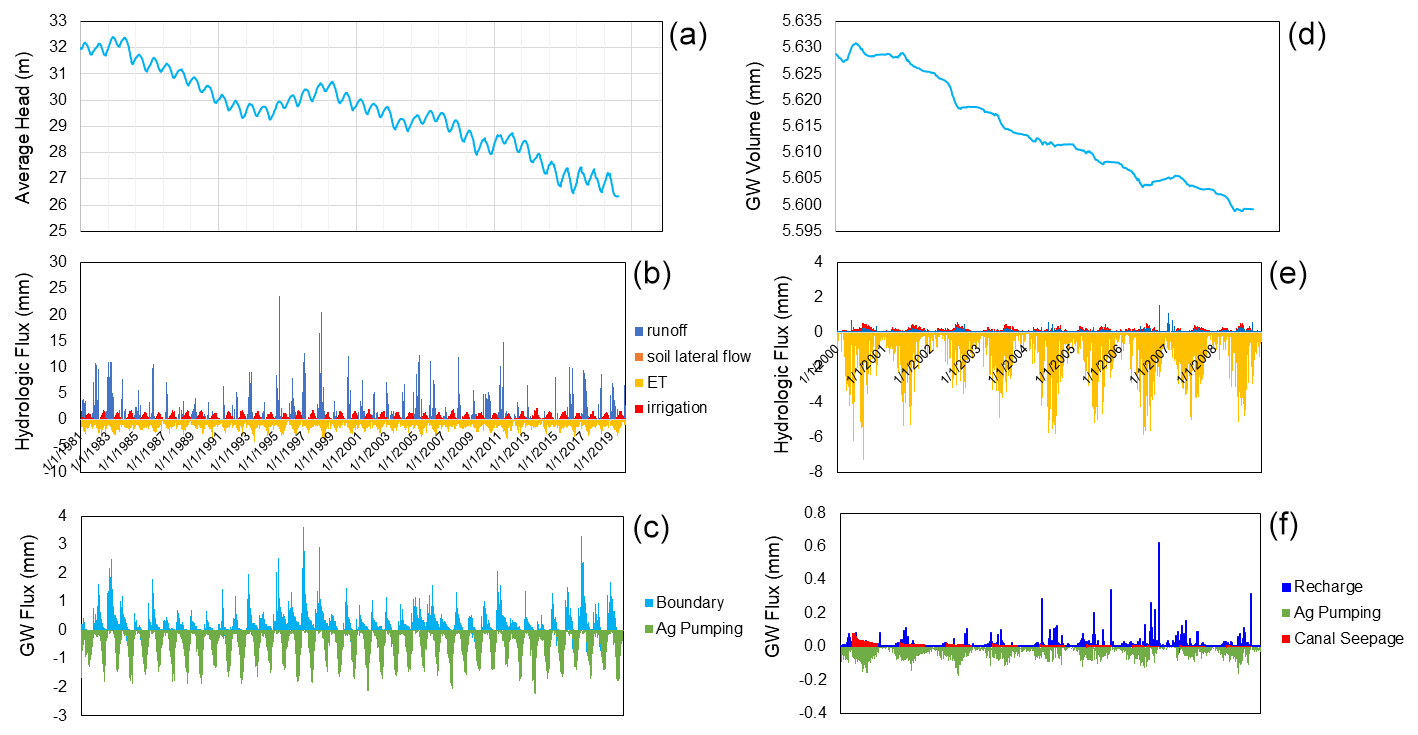
Figure 9 Time series of daily model output. Panels (a), (b), and (c) show average head from all monitoring well locations, major hydrologic fluxes, and major groundwater fluxes for the Joaquin River watershed; (d), (e), and (f) show groundwater volume, major hydrologic fluxes, and major groundwater fluxes for the John Martin Reservoir watershed.

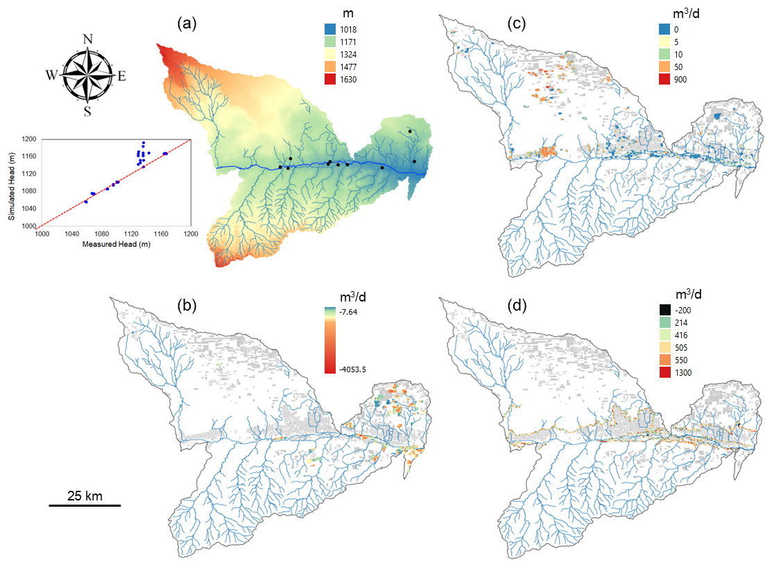
Figure 10 Maps of simulated SWAT+MODFLOW cell-by-cell results for the John Martin Reservoir Watershed, showing (a) groundwater head (m), (b) pumping for irrigation, (c) recharge, and (d) canal seepage for July 2008. For (a), the location of the USGS monitoring wells is shown with black dots, and a plot of simulated vs. measured groundwater head is shown next to the head map. For (b), (c), and (d), white areas indicate regions where volumetric flow rates = 0.

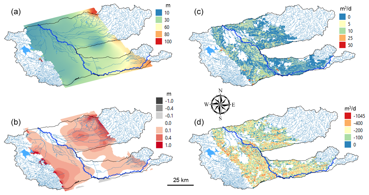
Figure 11 Maps of simulated SWAT+MODFLOW cell-by-cell results for the San Joaquin watershed, showing (a) groundwater head for the year 2018 (m), (b) average yearly change in head (m) between 1981 and 2018 (positive values = decrease in head), (c) average daily recharge for 2018, and (d) average daily irrigation pumping for 2018.

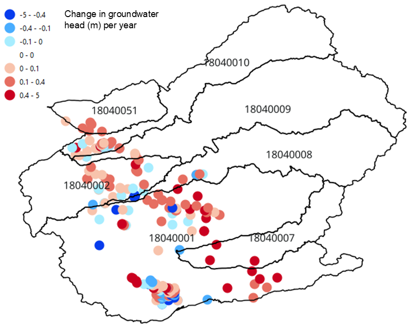
Figure 12 Average yearly change (1981–2018) in observed groundwater head (m yr⁻¹) for each USGS groundwater monitoring well within the San Joaquin River Basin, which contains the study region MSJ-LC (18040001). Red = decrease in head; Blues = increase in head.

3.3 Streamflow

Measured and simulated monthly streamflow are shown in Fig. 13 for the two study regions. For the Arkansas River within the JMR, the model replicates streamflow well (NSE = 0.89, 0.81), due to appropriate canal diversions and groundwater-channel exchange. For the San Joaquin River within the MSJ-LC, simulated streamflow in the upper reaches of the river (Mendota – 11254000) does not match measured streamflow to a reasonable degree (NSE = −0.31). However, simulated streamflow improves downstream, for the Fremont (NSE = 0.57) and Newman gage sites (NSE = 0.55), with the timing of peak flow and baseflow represented correctly. Peak flow for the five major events between 1981 and 2019 is underestimated by the model, which could be improved with further calibration of surface runoff in tributary watersheds.

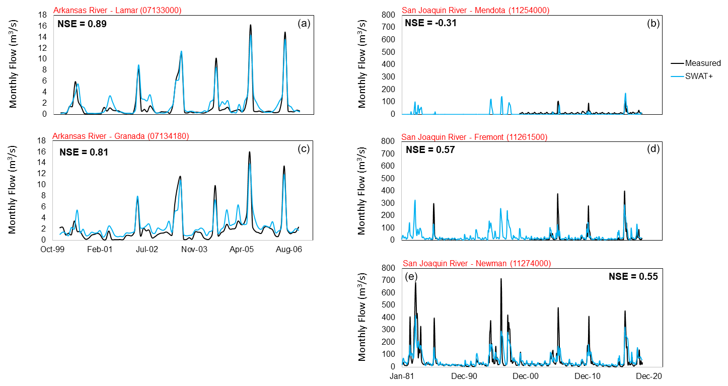
Figure 13 Monthly time series of measured and simulated streamflow at USGS streamflow gaging sites in the (a, c) John Martin Reservoir watershed and the (b, d, e) San Joaquin River watershed. The gage name and USGS site are shown in red for each plot. Also, the NSE value is shown on each plot.

3.4 Study limitations

The intent of this paper is not to provide calibrated models that can be used for scenario analysis. Rather, the objective is to present a new hydrologic modelling code, SWAT+MODFLOW, which can be used to simulate all major surface-subsurface hydrologic processes and fluxes within a watershed system in a physically based spatially distributed manner. Therefore, although the models presented here for the Arkansas River Basin and the San Joaquin River Basin perform reasonably well with expected results (e.g., decrease in groundwater head, canal seepage, groundwater pumping for irrigation), more calibration would need to be performed before application to scenarios such as management practices, climate, population growth, or policy changes. Other study limitations including the following:

Vadose zone hydrology. The model, as currently coded, does not include physically based unsaturated flow in the vadose zone between the bottom of the soil profile and the water table. Rather, a transfer function is used to route deep percolation water temporally to the water table. This limitation could be remedied using the Unsaturated Zone Flow (UZF) package (Niswonger et al., 2006), which could receive soil deep percolation as input and then route water through the vadose zone to the water table. This can be explored in later studies.

Confined aquifers. The models presented herein contain only unconfined aquifers. Although confined aquifers or aquifer systems with multiple layers can be included in MODFLOW, this feature was not explored in this study.

Channel-cell connections. Channel depths in SWAT+ can vary each daily time step but are uniform across the length of the channel. For long channels, this means that realistic spatially-dependent channel stages are not simulated with the model. Therefore, although groundwater head (m) can vary for each MODFLOW grid cell, each cell connected to a channel will use the same channel stage (m) to calculate the exchange rate with Darcy's Law. This limitation can be remedied by using short channels to delineate the stream system in the watershed. This was attempted in this study, by using NHD+ channel segments to represent the channel objects, resulting in 1324 and 2763 channels in the JMR and MSJ-LC models, respectively.

4 Conclusions

In this study, we present the SWAT+MODFLOW modelling code, a software tool that links the SWAT+ watershed model with the MODFLOW-NWT groundwater model, creating a single executable that can simulate surface-subsurface hydrological processes in a watershed system. The use of MODFLOW replaces the standard groundwater module of SWAT+, which treats groundwater movement and interaction with land surface features in a simplistic manner. SWAT+ simulates land surface hydrology, soil hydrology, and channel hydrology, whereas MODFLOW simulates groundwater hydrology and the interaction between groundwater and surface features (soils, canals, channels, reservoirs, tile drains, irrigation pumps). The model operates on a daily time step. Geographic connections between MODFLOW grid cells and SWAT+ objects (HRUs, channels, reservoirs) are created using a GIS and then listed in a set of input files to be read into the modelling code and then used during each daily time step to map variables (e.g., recharge, groundwater-channel exchange, groundwater-canal exchange, tile drainage outflow, pumping for irrigation) between SWAT+ and MODFLOW.

The modelling code is tested for accuracy and general application to two watersheds in semi-arid regions: the John Martin Reservoir (JMR) watershed in the Arkansas River Basin, Colorado; and the Middle San Joaquin – Lower Chowchilla (MSJ-LC) watershed in the Central Valley, California. The JMR watershed is distinguished by canal diversions, canal seepage, and surface water irrigation, whereas the MSJ-LC is distinguished by groundwater pumping for irrigation and resulting groundwater depletion. Model results are tested against monthly streamflow (m³ s⁻¹) at gaging station locations and annual groundwater head (m) at monitoring well locations, to demonstrate the model's capability in replicating historical hydrologic conditions to a reasonable degree. Further calibration can be performed if the models are to be used for scenario analysis.

The new SWAT+MODFLOW modelling code can be a helpful resource to researchers, engineers, and policy makers in studying water storage and movement and watersheds, and the impact of management practices, policies, and climate on surface water supply and groundwater supply in a physically based manner. As both SWAT+ and MODFLOW are widely used worldwide for watershed and groundwater modelling, we expect that this new tool can be an important asset in many water resources projects.