A framework for three-dimensional dynamic modeling of mountain glaciers in the Community Ice Sheet Model (CISM v2.2)

It is essential to improve our understanding of glaciers and their effects on sea levels, ecosystems, and freshwater resources in a changing climate. To this end, we implemented a framework for three-dimensional, high-resolution, regional-scale glacier simulations in the Community Ice Sheet Model (CISM v2.2), using higher-order ice-flow dynamics previously applied to the Greenland and Antarctic ice sheets. Here, we present the modeling framework and its application to the European Alps glaciers at a 100 m resolution, using protocols from the third phase of the Glacier Model Intercomparison Project (GlacierMIP3). The model results align with observations and other glacier models, indicating that Alpine glaciers will lose more than half their current mass if present-day climate conditions persist, with near-total loss under warmer scenarios. This new development integrates glacier and ice sheet systems in a common modeling framework and will support advances in coupled land ice–Earth system assessments across timescales in the Community Earth System Model (CESM).

1 Introduction

Numerical models are a powerful tool to study the physical processes governing glaciers and continental ice sheets, enabling the prediction of cryospheric changes from seasonal to millennial timescales and their impacts on Earth systems. These impacts span local, regional, and global scales and influence sea levels, hydroclimates, ecosystems, and human activities. For example, the Greenland and Antarctic ice sheets regulate global-scale climate and ocean circulation patterns and are major contributors to sea-level rise (Fox-Kemper et al., 2021). High-latitude (polar and sub-polar) glaciers, decoupled from the ice sheets, are also large contributors to sea-level rise and freshwater flux to the oceans (Hock et al., 2019; Marzeion et al., 2020; Zemp et al., 2019). Inland mountain glaciers contribute less to sea level but are important freshwater sources for streams, rivers, and lakes. These mountain glaciers regulate ecosystems, contribute to local and downstream water supply, and interact with regional hydroclimates on sub-seasonal to decadal timescales (Huss and Hock, 2018; Milner et al., 2009; Hock et al., 2005; Ficetola et al., 2024; Immerzeel et al., 2020; Bosson et al., 2023). Although the underlying physics of glaciers is similar to that of ice sheets, glaciers are usually studied with different models because of their smaller spatial scales. Modern ice sheet models typically have resolutions of ∼ 1 to 10 km, whereas mountain glaciers require sub-kilometer resolutions to accurately represent surface and bed topography, mass balance, and ice-flow dynamics.

Glacier mass balance (MB), geometry evolution, and ice-flow dynamics modeling has seen significant advancements over the past decade (Zekollari et al., 2022b), with the availability of global glacier inventories (RGI Consortium, 2017), distributed global- and regional-scale ice thickness estimates (Farinotti et al., 2019; Grab et al., 2021; Millan et al., 2022), and satellite-derived mass-balance measurements (Hugonnet et al., 2021). The representation of glacier geometry has evolved from the simplified volume–area/length scaling of early models (Bahr et al., 1997; Hock et al., 2019) to geometric models that dynamically adjust area and surface elevation at all elevations (Huss and Hock, 2015) and recently to two-dimensional flowline dynamics based on the shallow-ice approximation, for example, the Open Global Glacier Model (OGGM v1.1; Maussion et al., 2019) and the Global Glacier Evolution Model flow (GloGEMflow; Zekollari et al., 2019). Some newer developments include the 3D geometry of individual glaciers (e.g., GloGEMflow3D; Zekollari et al., 2022a). Advances in computational power and numerical techniques, such as GPU processing and machine learning (ML) approaches, have further enabled 3D models of glacier evolution over long timescales with improved resolution. For example, the Instructed Glacier Model (IGM) applies deep learning to emulate Stokes dynamics and predict the evolution of ice sheets, ice caps, and glaciers (Jouvet et al., 2021; Jouvet and Cordonnier, 2023). Other ML applications for glacier modeling have also been explored, including MB reconstruction (Guidicelli et al., 2023), MB uncertainty estimation (Diaconu and Gottschling, 2024), and ice-flow dynamics (Bolibar et al., 2023). However, applications of full-Stokes models (which solve the 3D Stokes equations for ice flow) to large regions and global-scale assessments have been limited due to computational requirements (Zekollari et al., 2022b, and the citations therein).

To provide a structured framework for comparing multiple glacier models, assessing their performance, and improving confidence in model projections, the Glacier Model Intercomparison Project (GlacierMIP) was launched in 2015. The first two phases of GlacierMIP focused on glacier evolution through the 21st century. GlacierMIP1 (2015–2019) compared published projections from six glacier evolution models (Hock et al., 2019). None of the six models included prognostic ice dynamics; instead, five models relied on volume–area/length scaling for geometry change (Slangen et al., 2011; Radić et al., 2013; Marzeion et al., 2012; Hirabayashi et al., 2013; Giesen and Oerlemans, 2013), and one model used an empirical glacier evolution scheme (Huss and Hock, 2015). Eleven models took part in GlacierMIP2 (2019–2020) (Marzeion et al., 2020), including the flowline models OGGM and GloGEMflow. The third phase, GlacierMIP3 (Zekollari et al., 2025), built on the first two phases and investigated the long-term equilibration of glaciers under constant climate conditions. In GlacierMIP3, the models have become increasingly sophisticated in terms of geometry representation, mass balance, and ice dynamics.

This study presents a new framework for simulating glaciers in the Community Ice Sheet Model (CISM), the ice dynamics component of the Community Earth System Model (CESM; Danabasoglu et al., 2020). Originally developed to simulate the evolution of the Greenland and Antarctic ice sheets (Lipscomb et al., 2019, 2021), CISM is the first 3D, higher-order ice-flow model to participate in GlacierMIP. In contrast to the 2D flowline models, which resolve the flow only in the x–z plane (where x is the direction of motion), CISM is a dynamic model that predicts the ice velocity, temperature, and stresses in three dimensions. As a higher-order model, it includes not only vertical shear stresses, but also longitudinal and lateral stresses, in the ice momentum balance (Hindmarsh, 2004; Pattyn et al., 2008). Integrating glacier modeling within an Earth system model (ESM) framework offers several emerging advantages for studying glaciated regions. It will enable dynamic coupling with the climate system, enhancing the representation of feedback mechanisms with the land–atmosphere–hydrology components. This integration will allow more comprehensive assessments of climate, ecological, and hydrological impacts across glaciated regions worldwide.

The new CISM developments support high-resolution, regional-scale glacier simulations, similar to those of other regional glaciation models (Seguinot et al., 2018; Clarke et al., 2015). This is in contrast to glacier-centric models, such as GloGEMflow3D and OGGM, that model each glacier independently. When run as a glacier model, CISM can compute and calibrate the surface mass balance (SMB) for all glaciers in the domain, optimize the agreement between modeled and observed glacier area and thickness, and track the advance and retreat of each glacier.

In this work, we apply the new glacier-enabled model to all the glaciers of the European Alps in the framework of GlacierMIP3. After reviewing CISM's ice sheet capabilities (Sect. 2), we describe the new developments that support glacier simulations and their implementation in relation to the European Alps (Sect. 3); discuss the model initialization, spin-up, and calibration process (Sect. 4); and present the results from the GlacierMIP3 experiments (Sect. 5). We then evaluate the computational performance (Sect. 6), discuss model limitations and future work (Sect. 7), and offer conclusions (Sect. 8).

2 CISM as an ice sheet model

CISM is a parallel, open-source code, written in Fortran and Python, which can be run either as a standalone ice sheet model or as a coupled component of CESM. As a standalone model, CISM has participated in several community comparisons, including the Ice Sheet Model Intercomparison Project (ISMIP6; Nowicki et al., 2020; Goelzer et al., 2020; Seroussi et al., 2020), the Linear Antarctic Response to basal melting Model Intercomparison Project (LARMIP2; Levermann et al., 2020), and the Antarctic Buttressing Model Intercomparison Project (ABUMIP; Sun et al., 2020). As a coupled CESM component, CISM has been used to study the evolution of the Greenland ice sheet in future climates (Muntjewerf et al., 2020a, b) and during the Last Interglacial period (Sommers et al., 2021).

Because glaciers and ice sheets share similar underlying physics, most of CISM's numerical algorithms can be applied to glaciers without modifications. This section summarizes methods common to ice sheets and glaciers, while Sect. 3 describes the new glacier-related developments.

2.1 Dynamical core

CISM includes a dynamical core, called Glissade, which solves conservation equations for mass, momentum, and thermal energy to determine changes in ice thickness, velocity, and internal temperature. The model runs on a structured rectangular grid with scalars (e.g., ice thickness and temperature) located at the cell centers and velocity components at cell corners. The most complex part of the dynamical core is a velocity solver that incorporates a hierarchy of Stokes-flow approximations, including (1) the shallow-ice approximation (SIA; Hutter, 1983), (2) the shallow-shelf approximation (SSA; MacAyeal, 1989), (3) a depth-integrated higher-order approximation (DIVA) based on Goldberg (2011), and (4) a higher-order approximation based on Blatter (1995) and Pattyn (2003).

With the Blatter–Pattyn (BP) approximation, CISM solves a 3D set of elliptic equations for the horizontal velocity components (u,v) at all vertical levels. DIVA simplifies the problem by solving a 2D set of elliptic equations for the vertically averaged velocity components $(\stackrel{\mathrm{‾}}{u},\stackrel{\mathrm{‾}}{v})$ in each ice column and then integrating vertically through each column to obtain the full 3D velocity profile (see Goldberg, 2011, and Lipscomb et al., 2019, for details). The DIVA solver is computationally much faster than BP, while it computes velocities similar to those of BP in most glaciated regions. An exception would be flow with large vertical shear over a bed with rough topography, as discussed by Goldberg (2011). In the runs below, most glaciers have relatively smooth beds and/or sliding-dominated flow with small vertical shear, for which the two solvers give similar results. DIVA also scales well to the high resolutions needed to model mountain glaciers (Robinson et al., 2022). We therefore used DIVA for the simulations in this study.

DIVA solves the following approximation of the Stokes equations in the x and y directions:

$$\begin{array}{}\text{(1)}& \begin{array}{rl}& {\displaystyle \frac{\mathrm{1}}{H}}{\displaystyle \frac{\partial }{\partial x}}\left[\mathrm{2}\stackrel{\mathrm{‾}}{\mathit{\eta }}H\left(\mathrm{2}{\displaystyle \frac{\partial \stackrel{\mathrm{‾}}{u}}{\partial x}}+{\displaystyle \frac{\partial \stackrel{\mathrm{‾}}{v}}{\partial y}}\right)\right]\\ & +{\displaystyle \frac{\mathrm{1}}{H}}{\displaystyle \frac{\partial }{\partial y}}\left[\stackrel{\mathrm{‾}}{\mathit{\eta }}H\left({\displaystyle \frac{\partial \stackrel{\mathrm{‾}}{u}}{\partial y}}+{\displaystyle \frac{\partial \stackrel{\mathrm{‾}}{v}}{\partial x}}\right)\right]+{\displaystyle \frac{\partial }{\partial z}}\left(\mathit{\eta }{\displaystyle \frac{\partial u}{\partial z}}\right)={\mathit{\rho }}_{i}g{\displaystyle \frac{\partial s}{\partial x}},\\ & {\displaystyle \frac{\mathrm{1}}{H}}{\displaystyle \frac{\partial }{\partial x}}\left[\stackrel{\mathrm{‾}}{\mathit{\eta }}H\left({\displaystyle \frac{\partial \stackrel{\mathrm{‾}}{u}}{\partial y}}+{\displaystyle \frac{\partial \stackrel{\mathrm{‾}}{v}}{\partial x}}\right)\right]\\ & +{\displaystyle \frac{\mathrm{1}}{H}}{\displaystyle \frac{\partial }{\partial y}}\left[\mathrm{2}\stackrel{\mathrm{‾}}{\mathit{\eta }}H\left({\displaystyle \frac{\partial \stackrel{\mathrm{‾}}{u}}{\partial x}}+\mathrm{2}{\displaystyle \frac{\partial \stackrel{\mathrm{‾}}{v}}{\partial y}}\right)\right]+{\displaystyle \frac{\partial }{\partial z}}\left(\mathit{\eta }{\displaystyle \frac{\partial v}{\partial z}}\right)={\mathit{\rho }}_{i}g{\displaystyle \frac{\partial s}{\partial y}},\end{array}\end{array}$$

where H is the ice thickness, $\stackrel{\mathrm{‾}}{\mathit{\eta }}$ is the vertical mean viscosity, ρ_i is the density of ice, g is gravitational acceleration, and s is the surface elevation. The three terms on the left side of the equation describe longitudinal stresses, lateral stresses, and vertical shear stresses. These internal ice stresses balance the gravitational driving force on the right-hand side.

The viscosity η is a nonlinear function of the temperature and strain rate:

$$\begin{array}{}\text{(2)}& \mathit{\eta }\equiv {\displaystyle \frac{\mathrm{1}}{\mathrm{2}}}{A}^{\frac{-\mathrm{1}}{n}}{\dot{\mathit{\epsilon }}}_{\mathrm{e}}^{\frac{\mathrm{1}-n}{n}},\end{array}$$

where A is a temperature-dependent flow factor, ${\dot{\mathit{\epsilon }}}_{\mathrm{e}}$ is the effective strain rate (derived from the 3D strain-rate tensor), and n=3 is the exponent in Glen's flow law. The ice velocity can be partitioned into a sliding velocity u_b and an internal deformational velocity. The lower the viscosity, the greater the deformational velocity relative to the sliding.

When solving Eq. (1), CISM has an option to cap the magnitude of the surface slope ($\Vert \partial s/\partial x\Vert$ at east and west cell edges and $\Vert \partial s/\partial y\Vert$ at north and south edges) at a value of m_max to maintain model stability in regions of steep topography. For this study we set m_max=1.0 (a 45° slope). The cap is applied to about 1 % of ice-covered cell edges in the Alps domain described in Sect. 4.

The model supports several basal friction schemes with different relationships between sliding velocity and shear stress. For the simulations in this study, the sliding velocity is computed using a Weertman-type power law (Weertman, 1957):

$$\begin{array}{}\text{(3)}& {\mathit{\tau }}_{\mathrm{b}}=C_p|{\mathit{u}}_{\mathrm{b}}{|}^{\frac{\mathrm{1}}{m}-\mathrm{1}}{\mathit{u}}_{\mathrm{b}},\end{array}$$

where τ_b is the basal shear stress (a boundary condition for Eq. 1), u_b is the basal sliding velocity, m is a power-law exponent, and C_p is a spatially varying friction coefficient.

2.2 Ice sheet initialization

Ice sheets are initialized in CISM by spinning up the model for thousands of simulated years until the ice geometry reaches a steady state consistent with the applied forcing. External forcing consists of the surface mass balance (which determines thickness changes at the upper ice surface), the surface air temperature (an upper boundary condition for ice thermodynamics), the geothermal heat flux (a lower boundary condition for the thermodynamics of grounded ice), and ocean thermal forcing in sub-ice-shelf cavities for floating ice. The climate forcing used during the spin-up is derived from observations or models and is typically from a period in the 20th century when the ice sheet was in approximate balance with the climate. During the spin-up, the ice sheet is nudged towards an observation-based thickness target (e.g., Morlighem et al., 2014, 2019). For grounded ice, this is done by adjusting a spatial field of friction coefficients in the basal sliding law (Pollard and DeConto, 2012; Lipscomb et al., 2021).

The initialization is followed by a historical run to advance the ice sheet state to the present day and then a projection run that continues into the future. Forcing during the historical run comes from recent observations and reanalyses, while the projection run uses output from simulations of future climate by regional models or ESMs.

3 CISM development for glacier modeling and application to the European Alps

3.1 Forcing and initialization data

CISM requires five types of input data for glacier simulations: the outline and ID of each glacier, continuous surface elevation over the domain, ice thickness, atmospheric forcing, and climatic mass balance.

1. We used the glacier outlines and IDs from version 6 of the Randolph Glacier Inventory (RGIv6; RGI Consortium, 2017). For the Alps, most glacier outlines are from summer 2003. We refer to this as the RGI date and use it as the reference year for the glacier extent.

2. To create continuous surface elevation, we used two digital elevation model (DEM) sources: (1) the USGS 3 arcsec (90 m) SRTM (Shuttle Radar Topography Mission) DEM and (2) finer-resolution glacier-specific surface DEM tiles taken from Farinotti et al. (2019) (hereafter F19). We merged these two sources, with the latter taking precedence in overlapping regions.

3. The target distributed ice thickness for calibration was taken from the F19 five-model consensus estimate.

4. The Inter-Sectoral Impact Model Intercomparison Project phase 3b (ISIMIP3b) W5E5 v2.0 data provided the atmospheric forcing at daily, 0.5° resolution from January 1979 through December 2019 (Lange et al., 2021). W5E5 is a merged dataset with WATCH Forcing Data methodology applied to ERA5 data (Cucchi et al., 2020). The variables needed for CISM are near-surface air temperature (°C), total precipitation flux (kg m⁻² s⁻¹), and surface elevation of the data (m). We averaged the atmospheric forcing to monthly mean values.

5. We used the glacier-wide geodetic mass balance from Hugonnet et al. (2021) for CISM SMB calibration.

Given that the W5E5 v2.0 forcing data began in 1979, we chose a 1984 baseline and calculated the 1979–1988 average to establish a baseline climatology, assuming approximate glacial equilibrium during this decade. We constructed a recent climatology (nominally for the year 2010) by taking the 2000–2019 mean, the same period over which Hugonnet et al. (2021) calculated the geodetic mass balance.

3.2 Model domain and resolution

The CISM domain for this study covers the European Alps (Fig. 1), with 3892 individual glaciers (out of 3927 glaciers in RGIv6 region 11). These glaciers cover a combined area of ∼ 2089 km². We excluded 35 small glaciers in the Pyrenees, Montenegro, and Albania (combined area of ∼ 3 km², i.e., ∼ 0.1 % of the regional area) that were in the original RGIv6 region 11 to reduce the model domain size. The two largest glaciers in the domain are the Aletsch (∼ 82 km²) and Gorner (∼ 56 km²), while more than 40 % of the glaciers have areas smaller than 0.05 km². Therefore, the model grid must be fine enough to accurately represent these small glaciers and their flow dynamics.

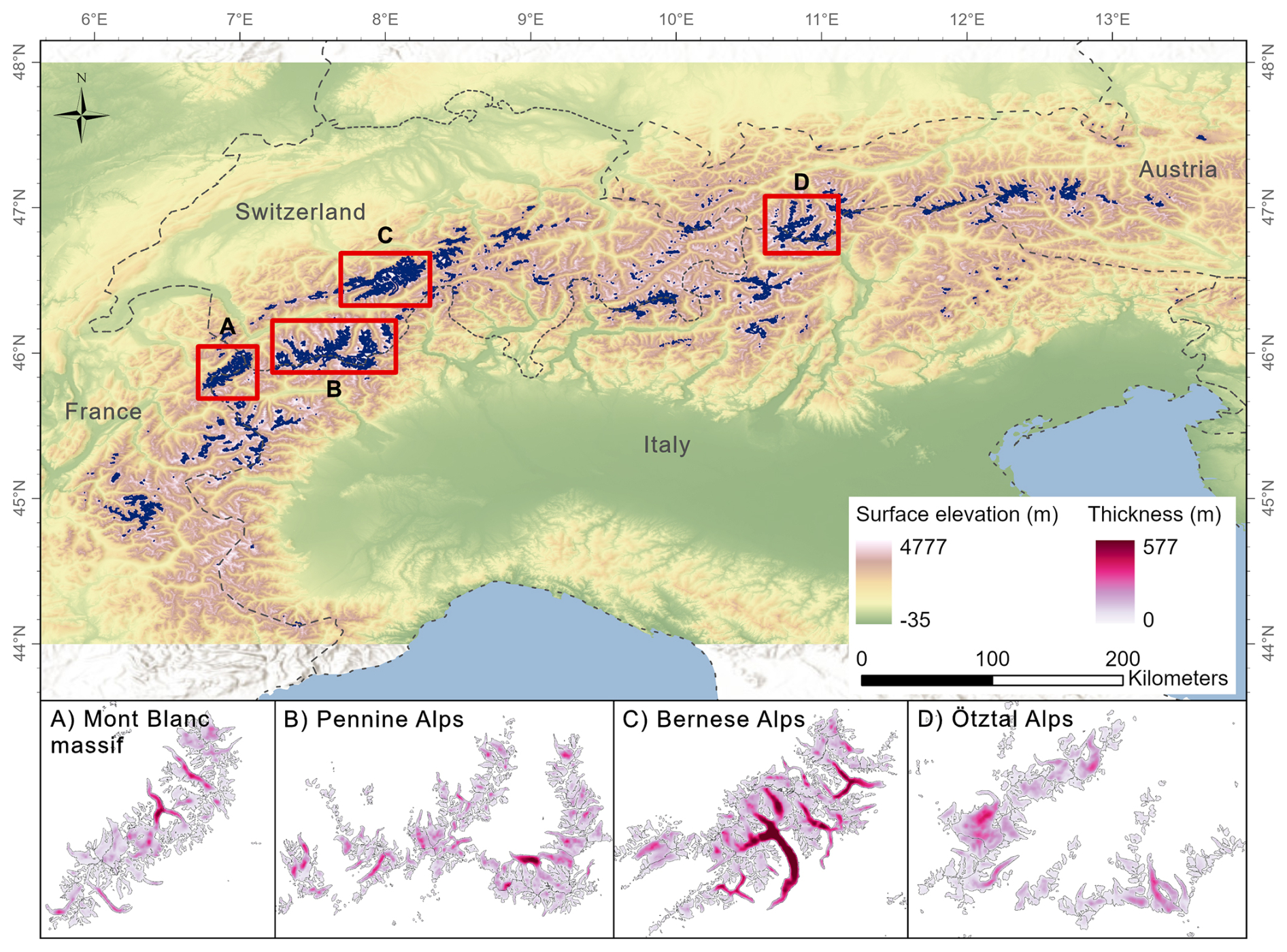
Figure 1 Top: CISM domain for the European Alps, which contains most of the glaciers in RGI region 11 (Central Europe). Shading shows the surface elevation profile (m). Bottom: input ice thickness (m) from Farinotti et al. (2019), remapped to the 100 m CISM grid, for four sub-domains (A–D).

We created two grids with horizontal resolutions of 100 and 200 m, using the coarser grid for model development and the finer grid for GlacierMIP3 production runs. At 100 m resolution, six glaciers are at subgrid scale, leaving 3886 glaciers resolved; 42 of these occupy a single grid cell. The 200 m grid resolves 3633 glaciers, with around 780 glaciers occupying a single model grid cell. All results in this study use the 100 m grid; Sect. 6 discusses the computational costs associated with both resolutions.

3.3 Glacier identification and tracking

Each glacier in the RGIv6 inventory has a unique identification number. The first step to modeling these glaciers is to remap the RGI outlines to the CISM grid and assign an RGI ID to each grid cell with a nonzero ice thickness. At startup, CISM makes a list of all the unique RGI IDs in the domain. It puts these in numerical order and associates each RGI ID with a CISM glacier ID between 1 and N_g, where N_g is the total number of glaciers. Numbering the glaciers in order without gaps facilitates calculations that require looping over all glaciers.

Cells that are initially ice-free receive a CISM ID of 0. When a glacier retreats, all new ice-free cells are also given an ID of 0. If the glacier re-advances to a cell from which it previously retreated, the initial ID is restored. Some glaciers will advance into cells that were initially ice-free; a cell is deemed to be newly glaciated when its ice thickness H exceeds a prescribed value H_min. When this happens, CISM looks upstream to the grid cells that are ice sources for the new glacier cell. In most cases, the upstream ice belongs to a single glacier, which provides the ID for this cell. If the upstream ice belongs to two different glaciers, CISM must choose between them. We found that selecting the upstream glacier ID that yields a more negative SMB for the new glacier cell is optimal, as a negative SMB inhibits further advance beyond the original RGI boundary.

3.4 Glacier surface mass balance

When run as an ice sheet model, CISM usually does not compute the SMB internally. Instead, the SMB is an input from a regional climate model, or it is computed at runtime by the land component of CESM when interactively coupled. For CISM as a glacier model, coupling between the land and land ice components of CESM has not yet been implemented. Therefore, we introduced a simple temperature-index method in CISM to calculate the SMB, which is similar to the scheme in OGGM (Maussion et al., 2019).

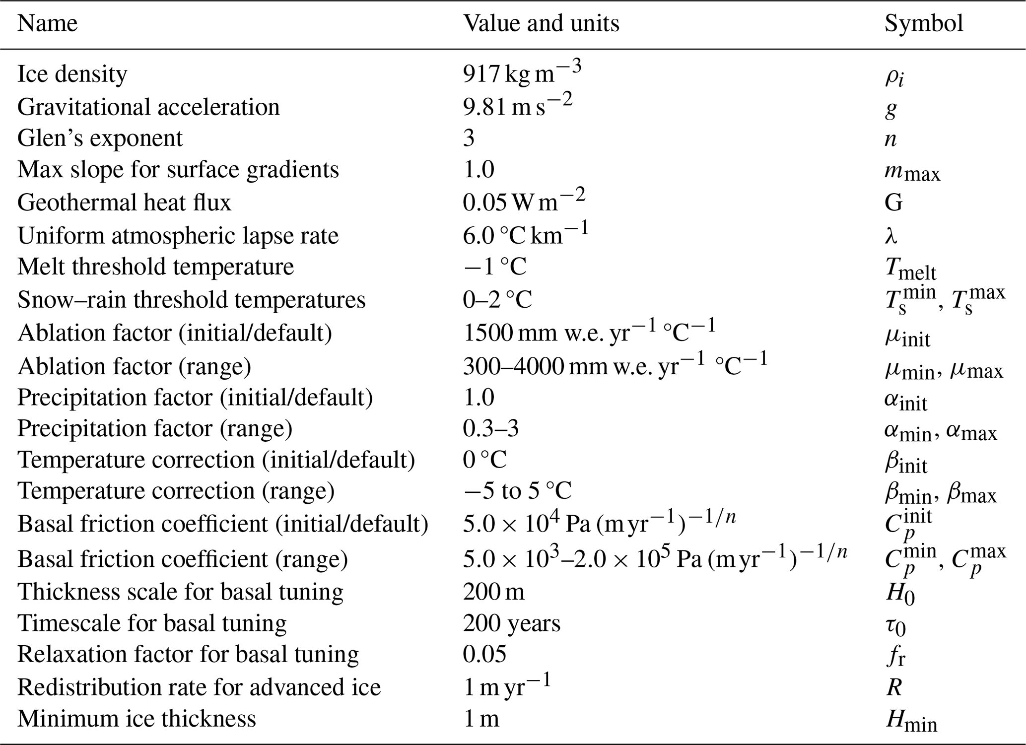
In this scheme, CISM computes the SMB of glaciers based on the monthly mean surface air temperature and precipitation rate, remapped to the CISM grid. The input air temperature is usually provided at the reference elevation of the coarse-resolution atmospheric forcing. CISM downscales the air temperature from the reference elevation to the local surface elevation on the high-resolution model grid based on a fixed lapse rate λ (Table 1). The fraction of the total precipitation reaching the glacier surface as snow depends on the downscaled temperature T. Precipitation is assumed to fall entirely as snow when $T<=T_{\mathrm{s}}^{\min }$ and as rain when $T\mathit{>=}{T}_{\mathrm{s}}^{\max }$. At temperatures between $T_{\mathrm{s}}^{\min }$ and $T_{\mathrm{s}}^{\max }$, the snow fraction varies linearly between 1 and 0. The SMB is calculated as the difference between snowfall and snowmelt, estimated using a temperature-index scheme:

$$\begin{array}{}\text{(4)}& B_i=\mathit{\alpha }{S}_i-\mathit{\mu }\max (T_i-T_{\mathrm{melt}},\mathrm{0}),\end{array}$$

where B_i is the SMB for grid cell i, S_i is the snowfall rate, T_i is the surface temperature, and T_melt is a temperature threshold for melting. The quantities B_i, S_i, and T_i are monthly means at a given location. The units of B_i and S_i are mm water equivalent (w.e.) yr⁻¹, and T_i is measured in °C. Within the model, the ablation factor μ (also known as the degree-day factor, melt factor, or temperature sensitivity parameter in the literature) is computed in mm w.e. yr⁻¹ °C⁻¹, while the precipitation correction parameter α is dimensionless. Section 4.3 describes the mass-balance calibration in detail.

Table 1 Default values of various physical constants and glacier-specific parameters in CISM. These parameters are user-defined and can be adjusted during the initial model setup.

4 Model initialization and calibration

4.1 Spin-up and historical runs

To initialize the model, we use a procedure similar to the method described for ice sheets in Sect. 2.2. That approach, however, relies on the area and thickness targets being appropriate for a steady state in equilibrium with the climate. Most glaciers have been losing mass in recent decades and are out of balance with the climate (Zemp et al., 2019; Zekollari et al., 2020), which means that estimates of present-day or recent ice thickness are not a suitable target for a steady-state spin-up. We therefore divide the initialization into two parts.

The first part is a spin-up run of several thousand years, with the forcing corresponding to a baseline climatology when glaciers are assumed to be approximately in equilibrium with the climate. Our simulations for the Alps used a 5000-year spin-up; the basal friction parameter C_p was inverted for the first 4000 years, then held constant for the final 1000 years to avoid initialization shocks in the forward runs. This is roughly the time needed for glacier thickness to reach a steady state. The total glacier volume changes by less than 0.03 km³ during the last 1000 years of the inversion and by less than 0.01 km³ during the period with constant basal parameters.

The second part is a historical run from the baseline year (1984; Sect. 3.1) to the outline date for glaciers in the RGIv6 dataset (∼ 2003). During the historical period, most simulated glaciers lose mass, consistent with the observational record. The goal of the spin-up is to initialize each glacier with an extent and thickness corresponding to the baseline year. If we lack region-wide observations for this year (as is usually the case), we make two approximations:

1. The areal retreat between the baseline year and the RGI year is relatively small; thus, we can use the unmodified RGI outlines as an area target. This assumption is undesirable for glaciers that retreated substantially between the baseline and RGI dates, but we considered it preferable to guessing the earlier outlines without observational support.

2. The decrease in thickness at a specific location from the baseline year to the RGI year can be estimated by calculating the average SMB between these two years. We accordingly adjust the target thickness, assuming that the SMB evolves linearly over time and that the time between the baseline and RGI dates (i.e., ∼ 19 years) is relatively short compared to the glacier's dynamic response time.

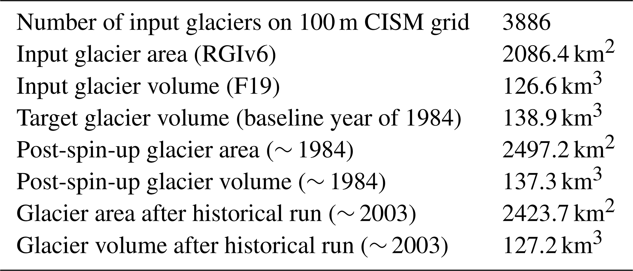
With the second assumption, we can adjust the baseline thickness targets at runtime to be consistent with the calibrated historical SMB. In a warming climate, the total ice volume will be greater at the baseline date than at the RGI date. When the model is run forward with the historical SMB, the goal is to reach the observed volume at the RGI date (Table 2), as specified in the GlacierMIP3 protocol. The methods for thickness inversion and mass-balance calibration are detailed below; Table 1 lists the various parameter values used here.

Table 2 Cumulative statistics for glaciers in the European Alps for the input data, at the end of the spin-up (1984), and for the RGI date (2003).

4.2 Thickness inversion

We compute the basal shear stress as a function of the sliding speed using Eq. (3). Because the friction coefficient C_p is not well constrained, we use it as a tuning parameter to nudge the ice thickness in each grid cell towards the baseline target. The value of C_p is initially set to $C_p^{\mathrm{init}}$ and is constrained to lie in the range [$C_p^{\min }$, $C_p^{\max }$] (Table 1). Where the ice is thicker than its target value, C_p is reduced to increase sliding and promote thinning, whereas C_p is increased if the ice is thinner than its target. The rate of change of C_p is given by

$$\begin{array}{}\text{(5)}& \begin{array}{rl}& {\displaystyle \frac{\mathrm{dlog}\left(C_p\right)}{\mathrm{d}t}}=\\ & \left[{\displaystyle \frac{(H_{\mathrm{obs}}-H)}{H_{\mathrm{0}}{\mathit{\tau }}_{\mathrm{0}}}}-{\displaystyle \frac{\mathrm{2}}{H_{\mathrm{0}}}}{\displaystyle \frac{\mathrm{d}H}{\mathrm{d}t}}-{\displaystyle \frac{f_{\mathrm{r}}}{{\mathit{\tau }}_{\mathrm{0}}}}\log (C_p/C_p^{\mathrm{init}})\right],\end{array}\end{array}$$

where H_obs is the thickness target, H₀ is a thickness scale, τ₀ is a relaxation timescale, and f_r is a relaxation factor. The first term on the right side minimizes differences between H and H_obs, the second term damps oscillations in C_p as H approaches H_obs, and the last term prevents C_p from drifting towards the max or min value when the first term is small but nonzero. The logarithmic form reflects the fact that a given change ΔC_p has greater dynamic effects when C_p is small than when C_p is large.

In most regions, this tuning procedure yields a steady-state ice thickness close to the target value. The procedure cannot, however, add ice to grid cells that are ice-free for other reasons (e.g., a highly negative SMB). Nor can it remove ice from cells that advance beyond the RGI outlines, but it gives these cells a low C_p that reduces the thickness. An alternate approach, often used in SIA glacier models, is to tune the softness parameter A in the ice viscosity, Eq. (2) (Zekollari et al., 2022b). In our CISM simulations, A is not a tuning parameter but determined internally by the evolving ice temperature.

The ice volume at the end of the 5000-year spin-up (nominally in 1984) is 137.3 km³, about 1 % below the target volume of 138.9 km³ (Table 2). The root-mean-square error between the modeled and target ice thickness across the entire ice-covered domain is 12.5 m. Positive differences (where the CISM thickness exceeds the target value) occur along glacier peripheries and at termini (Fig. 2). There are some regions where the modeled ice is thinner than the target value, which we discuss further in Sect. 7. During the historical run from 1984 to 2003, the volume decreases by about 8 % to 127.2 km³, within 0.5 % of the total F19 volume of 126.6 km³ (Table 2).

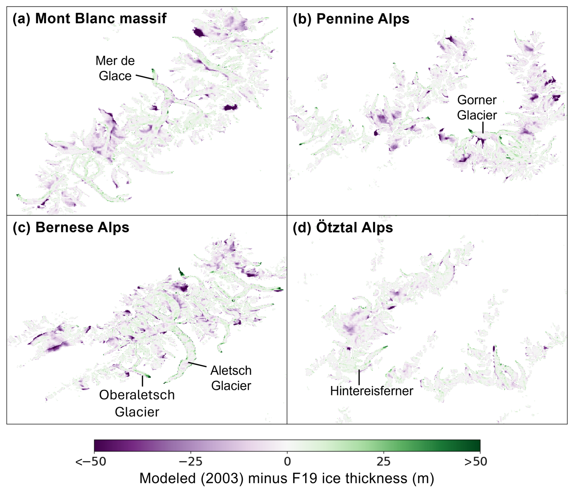
Figure 2 Difference between the post-calibration 2003 CISM and F19 ice thickness (m) for the four sub-domains in Fig. 1. Purple colors correspond to lower thickness in the CISM simulation.

The glaciers simulated in CISM have a total area of 2423.7 km² in 2003, greater than the RGI area of 2086.4 km². We attribute the excess area to two main factors. First, there is some numerical diffusion of ice thickness under transport. This can lead to one or two rows of advanced ice, usually no more than a few meters thick, at glacier peripheries (Fig. 2). To limit this spurious advance, we impose two corrections. In advanced cells (i.e., cells that are ice-covered in the model but are ice-free in the RGI data), we allow ablation where the computed SMB is negative, but we forbid accumulation where the computed SMB is positive. At the same time, we remove ice from advanced cells at a rate R and spread this ice, conserving mass, over the target area of the glacier. This can be viewed as a crude model of mass redistribution by avalanches on steep glacier walls. A redistribution rate R=1 m yr⁻¹ is enough to significantly reduce glacier advance. We do not, however, apply a negative SMB to advanced grid cells in the accumulation zone, as this would be a nonphysical sink for ice mass. Secondly, in CISM, ice can accumulate at high elevations on steep slopes. Though the avalanche redistribution process removes some of the peripheral ice, a portion remains, resulting in a larger area after spin-up.

We also ran the model forward from the RGI date to 2018 to compare the modeled 2018 ice thickness with the Grab et al. (2021) thickness measurements in the Swiss Alps, which used aerial ground-penetrating radar to determine ice thickness during 2016–2020. A direct comparison between the two datasets is not possible since the CISM extent is simulated, while the Grab et al. (2021) extent is observed (hence the two have different glacier outlines), but we found similar magnitudes and spatial patterns in thickness (Fig. 3).

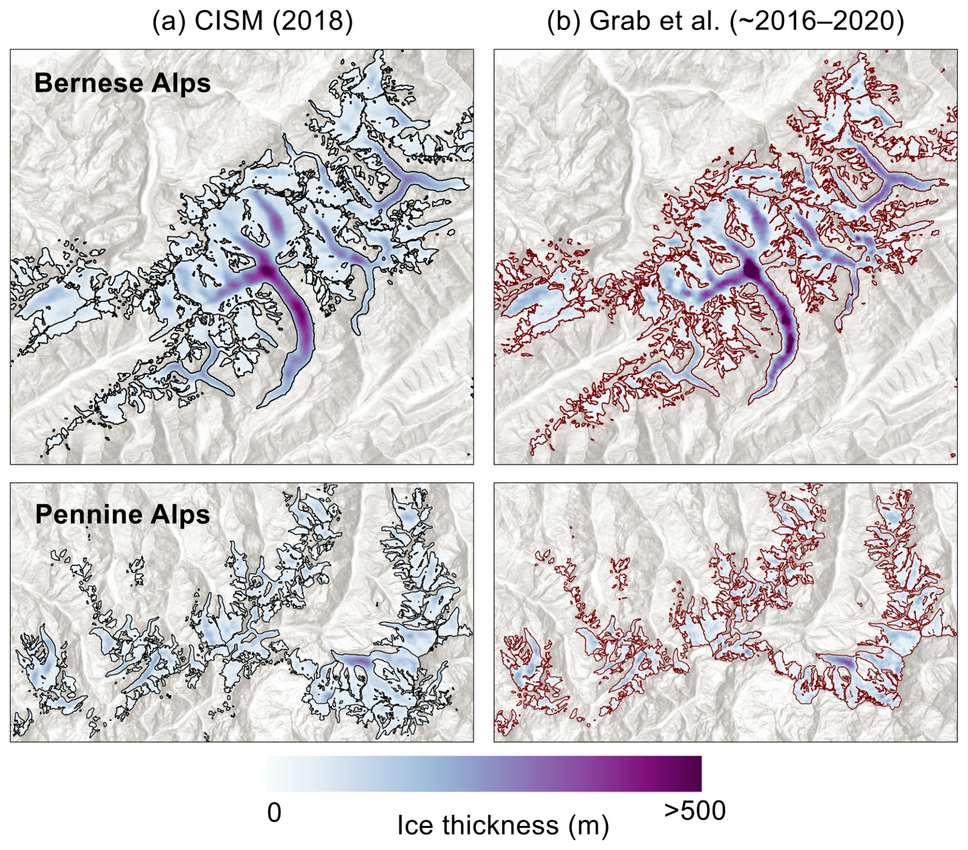
Figure 3 Comparison of CISM-simulated ice thickness (m) to observed thickness from Grab et al. (2021) for the Swiss Bernese and Pennine Alps around 2018. Note that the model and observations have different glacier extents in black and brown outlines, respectively.

4.3 Mass-balance calibration

The SMB parameters μ and α in Eq. (4) are calibrated for each glacier to yield a balanced state for the 1979–1988 climate while matching the Hugonnet et al. (2021) geodetic mass balance over 2000–2019. This is done in a two-step calibration process.

1. We assume that the glacier was in a state of approximate balance with the climate during a baseline period in the 20th century (i.e., the glacier-specific mean SMB was zero):

   $$\begin{array}{}\text{(6)}& B=\sum _{m=\mathrm{1}}^{\mathrm{12}}\sum _{i=\mathrm{1}}^N\left[\mathit{\alpha }{S}_{\mathrm{im}}-\mathit{\mu }\max (T_{\mathrm{im}}-T_{\mathrm{melt}},\mathrm{0})\right]=\mathrm{0},\end{array}$$

   where B is the annual-mean SMB for the glacier, the first summation is over the months of the year, the second summation is over the N grid cells in the glacier, and the subscript m denotes a particular month. For a given value of α (e.g., α=1 if the precipitation is unbiased), we can sum over all months and grid cells in Eq. (6) and obtain μ for each glacier.

2. If we have observations of both SMB and atmospheric forcing during a recent period when the glacier was out of balance with the climate, we introduce a second criterion. For each glacier we supplement Eq. (6) with a similar equation for the recent period:

   $$\begin{array}{}\text{(7)}& \widehat{B}=\sum _{m=\mathrm{1}}^{\mathrm{12}}\sum _{i=\mathrm{1}}^N\left[\mathit{\alpha }{\widehat{S}}_{\mathrm{im}}-\mathit{\mu }\max ({\widehat{T}}_{\mathrm{im}}-T_{\mathrm{melt}},\mathrm{0})\right],\end{array}$$

   where the carets denote quantities taken over the recent period.

Equations (6) and (7) form a system of two equations with two unknowns, which can be solved for α and μ for each glacier.

The summation over N cells for each glacier includes all the cells belonging to the glacier based on the RGI outlines, as well as ice-free cells bordering the glacier outline (within one cell) provided the bordering cells are in the ablation zone. In calculating the glacier's area-integrated annual-mean SMB, we include these neighboring cells because ice flows into and melts within them during at least part of the year. If these cells were excluded, the temperature sums in Eqs. (6) and (7) would be too small, and μ would be overestimated as a result.

The parameters α and μ are required to fall within physically reasonable ranges [α_min,α_max] and [μ_min,μ_max]. For some (usually small) glaciers, the α and μ computed from Eqs. (6) and (7) can lie outside these ranges because of atmospheric forcing biases or observational errors in $\widehat{B}$. In such cases, the first option is to ignore Eq. (7), set α to its default value of 1.0, and solve Eq. (6) for μ. This is done, for example, if $\widehat{B}>\mathrm{0}$ (i.e., the glacier is supposedly gaining mass) in a warming climate. If this first option fails to yield μ within the defined range, a second option is to introduce a temperature correction β, which is added to T_i for each cell in the glacier. This option is needed if T has a strong cold bias, resulting in little or no ablation even when μ is large.

Figure 4 shows the distribution of the calibrated parameters and the β correction for all glaciers in the domain. The μ values are limited to a range between 300 and 4000 mm w.e. yr⁻¹ °C⁻¹ (approximately 0.8–11 mm w.e. d⁻¹ °C⁻¹), and α values are limited to a range between 0.3 and 3 (Table 1). The correction β can be of either sign and is limited to a magnitude of 5 °C. These ranges are similar to, and somewhat narrower than, those in OGGM assessments. For example, Schuster et al. (2023) set the corresponding μ range to 0.33–33 mm w.e. d⁻¹ °C⁻¹, α range to 0.1–10, and β range to −8 to 8 °C. In our simulations, μ has a median value of 2.9 and a mean of 3.2 ± 1.8 mm w.e. d⁻¹ °C⁻¹ across all glaciers (without weighting according to glacier area or volume). More than 95 % of the glaciers have μ<6.3, which aligns with the previous literature. For example, Hock (2003) reported this parameter (referred to as the degree-day factor) ranging from 5–12 mm w.e. d⁻¹ °C⁻¹ for individual glaciers globally, while Braithwaite and Hughes (2022) reported values ranging from 4.1–6.8 for eight glaciers in the Alps. Schuster et al. (2023) assessed various temperature-index models and calibration methods and found a range for calibrated μ of ∼ 4–10 mm w.e. d⁻¹ °C⁻¹ for 88 glaciers globally.

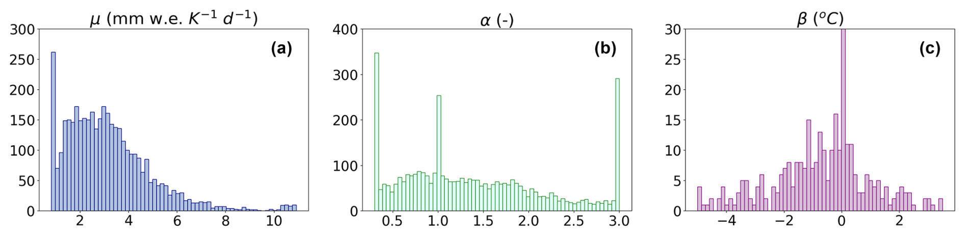
Figure 4 Distribution of the SMB parameters for all simulated glaciers in the Alps. The x axis shows the range of values for each parameter (Table 1), and the y axis shows the number of glaciers. The y axis in panel (c) is capped at 30 because most glaciers (n=3593) have β=0.

The median value of α is 1.22 (Fig. 4b). There are 304 glaciers with the lower threshold value of 0.3 and 273 glaciers with the upper value of 3.0, suggesting that some of these glaciers require a temperature correction β. We find that 293 glaciers have nonzero β (Fig. 4c), but all have values well within the ±5 °C threshold. Several factors, including variations among different glacier tributaries, as well as biases in the climate forcing and geodetic mass balance, influence the ranges of these glacier-specific parameters.

4.4 Surface velocity

We compared the modeled surface velocities with two satellite-derived estimates: ITS-LIVE (Gardner et al., 2022) and Millan et al. (2022), both remapped to the CISM grid (Fig. 5). Although velocity is not an inversion target, the simulated surface velocities are in good agreement with observations, showing that CISM is capturing key processes governing ice flow.

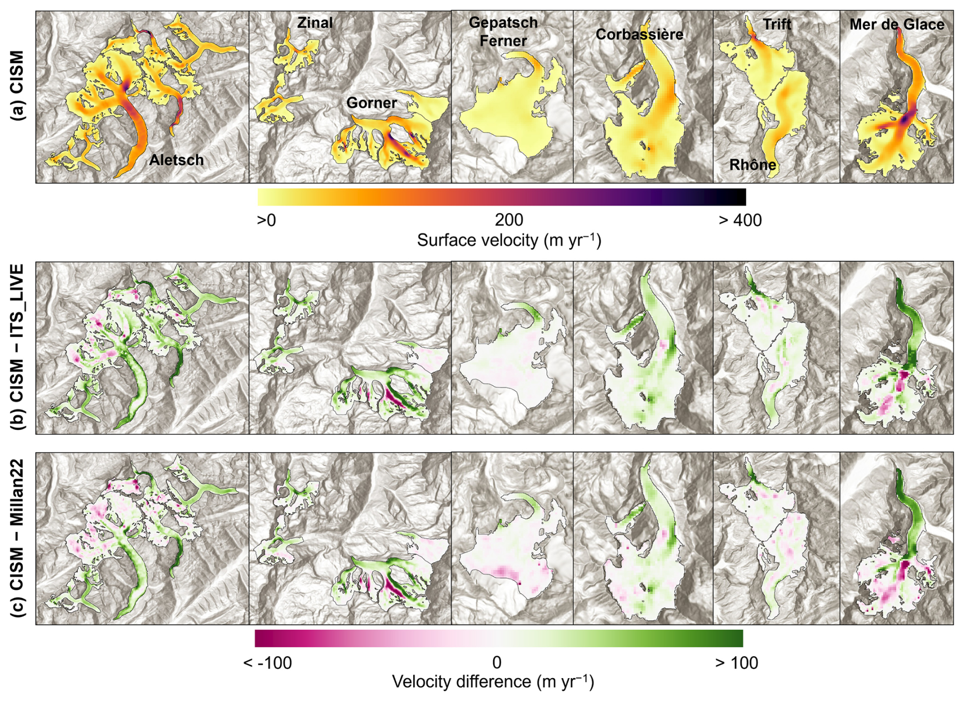
Figure 5 (a) CISM-simulated surface velocity (m yr⁻¹) for select large glaciers in the Alps. (b, c) Difference between CISM and two satellite-derived estimates: ITS-LIVE and Millan et al. (2022). All three velocity profiles are around the year 2017.

Figure 5 shows simulated and observed velocity patterns for several large glaciers, where velocity differences are generally more prominent due to the greater surface area and thickness. Because the Millan et al. (2022) data span 2017–2018, we limited our comparison of the three datasets to 2017, although seasonal velocity changes may cause some temporal misalignment. The model captures both the spatial patterns and the overall magnitudes quite well. However, the model–data differences can be greater for large glaciers, especially in accumulation zones and glacier tongues, where the model tends to overestimate velocities, and for higher elevations and upper tributaries, where it underestimates them (Fig. 5b, c). Statistically, the differences between CISM and the two datasets are small. Figure 6 illustrates this for ITS-LIVE and Millan et al. (2022), respectively, focusing on the largest glaciers that also have the greatest velocity differences. For cell-by-cell comparison, the mean differences are 19±35 and 11±34 m yr⁻¹ for the two datasets. Less than 10 % of the area has a difference exceeding ±50 m yr⁻¹. There could be several reasons for these differences, but in general, velocity errors are correlated with thickness errors. Where the model underestimates (overestimates) ice thickness, the driving stress and the ice speed are likely to be too low (high).

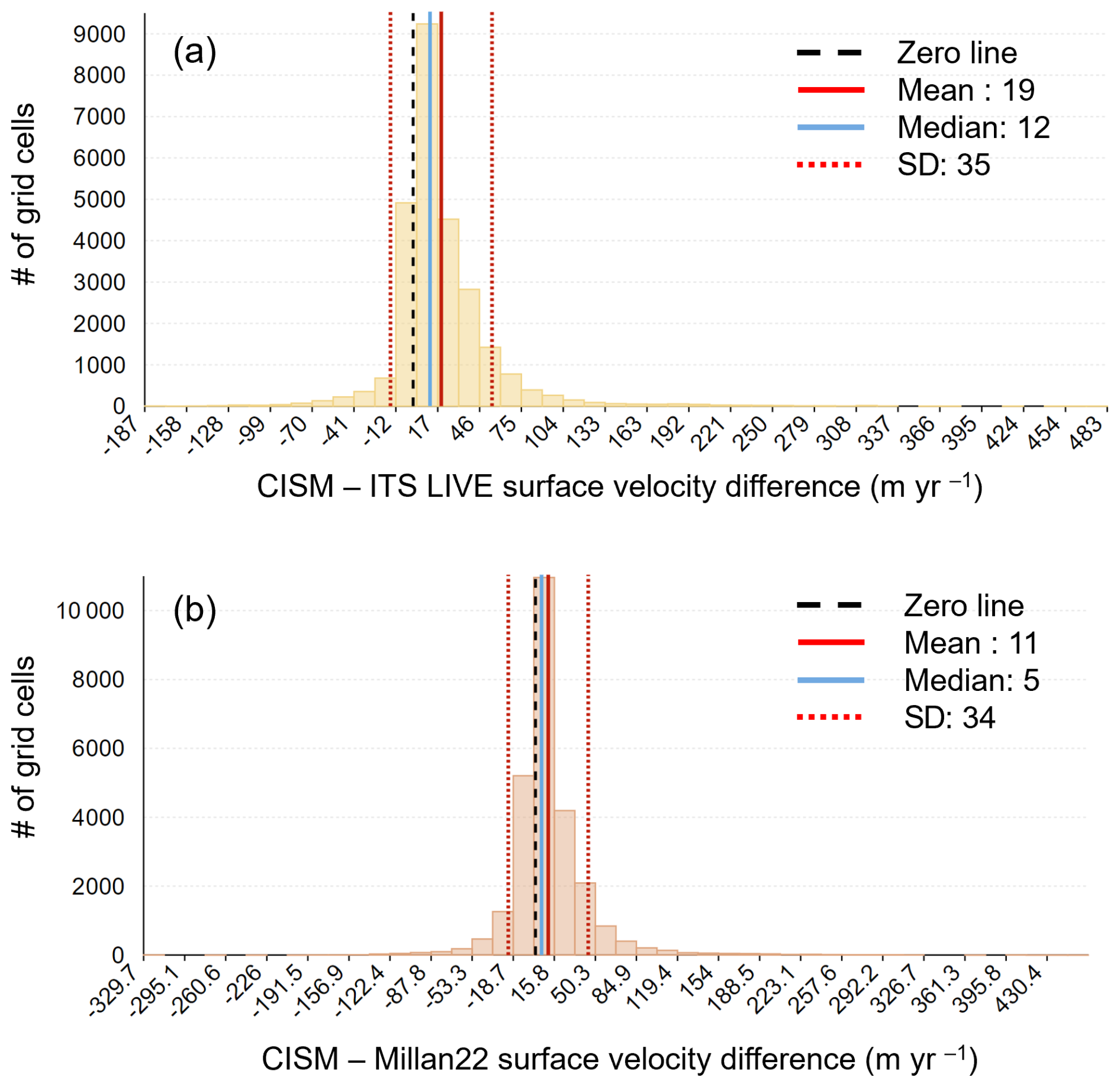
Figure 6 Velocity difference statistics between CISM and (a) ITS-LIVE and (b) Millan et al. (2022), around the year 2017. These are cell-by-cell differences for the 16 largest glaciers in the domain, each with an area > 14 km². The limits of the x axis correspond to the maximum difference.

5 GlacierMIP3 simulations

The goals of GlacierMIP3 were to (1) estimate the equilibrium area and volume of all glaciers outside the two ice sheets if temperatures were to stabilize at present-day levels, (2) make similar estimates for temperature changes under various climate change scenarios, and (3) determine the time needed to reach a new equilibrium. The GlacierMIP3 protocol specifies that each glacier should be initialized to its observed state on the RGI date. After initialization, each glacier is run forward to equilibrium for either 2000 years or 5000 years, depending on the region. Further details on the protocols and the prescribed atmospheric forcing are available on the GlacierMIP3 GitHub page (https://github.com/GlacierMIP/GlacierMIP3, last access: 24 January 2025).

5.1 Committed ice loss

We assessed the committed ice loss for glaciers in the Alps, i.e., the long-term equilibrium ice loss if recent climate conditions (2000–2019) were to remain unchanged. For the commitment run, we started with the baseline state of 1984 and gradually introduced warming from 1984–2010 using a linear ramp. After 2010, we held the atmospheric forcing constant and continued the simulation to 2484 (a total of 500 years), by which time the mass stabilizes.

Figure 7 shows snapshots for the Swiss Bernese Alps (including the Aletsch Glacier) for four dates: the 1984 baseline, 2021, 2084, and 2184. By 2184, the glaciers are close to equilibrium. Even in this highly optimistic climate scenario, there is significant area and volume loss (Fig. 7d), emphasizing that glaciers are far from equilibrium with the current climate. During this 200 years, the total ice volume drops from 137 km³ (1984) to 127 (2003), 105 (2021), 65 (2084), and 53 (2184). The total area drops from 2497 km² in 1984 to 1117 km² by 2184. At the end of the run in 2484, the area and volume are 1041 km² and 51 km³.

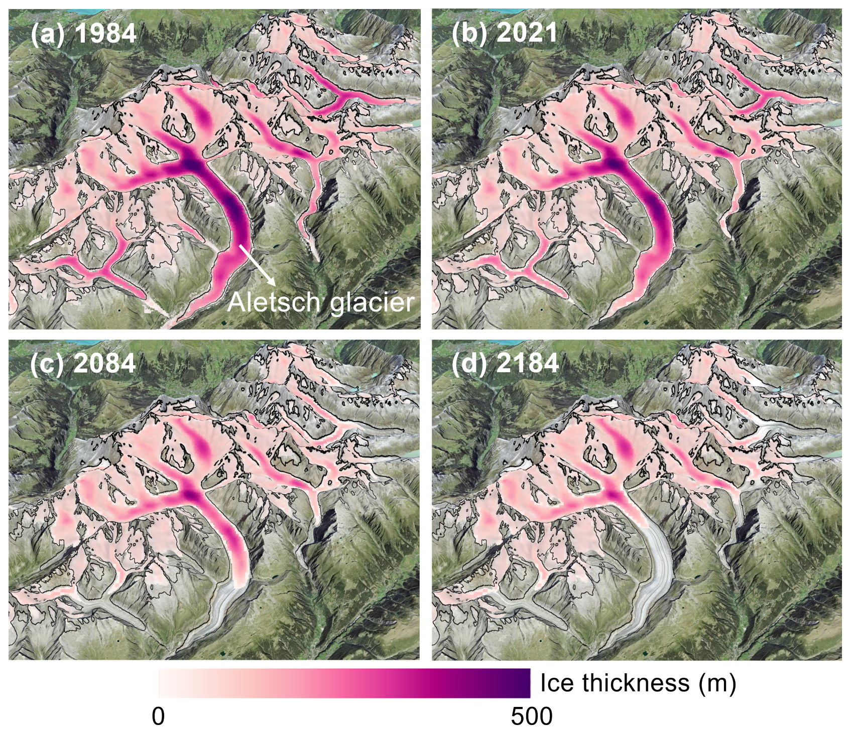
Figure 7 Committed ice loss for the Bernese Alps. Ice thickness (m) for (a) the baseline climate of 1984, and (b–d) years 2021, 2084, and 2184, assuming continuation of recent climate (2000–2019) with no further warming. RGIv6 glacier outlines (∼ 2003) are shown in black.

These results are similar to those of Jouvet and Huss (2019), who studied the retreat of the Aletsch Glacier using a full-Stokes ice dynamics model. They found that, by 2100, the Aletsch Glacier is already committed to losing nearly half its 2017 volume based on the 2008–2018 climate, with a 32 % loss projected using the 1988–2018 climate. CISM projects comparable volume loss with the 2000–2019 climate: approximately 34 % between 2017 and 2100. By 2017, the simulated Aletsch Glacier has already lost 11 % of its 1984 baseline volume of 14.30 km³.

5.2 Equilibration runs

We carried out the full suite of GlacierMIP3 experiments for the Alps glaciers in RGI region 11 (Fig. 1). Climate forcing for these experiments comes from five bias-corrected CMIP6 models from ISIMIP3b (GFDL-ESM4, IPSL-CM6A-LR, MPI-ESM1.2-HR, MRI-ESM2.0, and UKESM1-0-LL), for both the historical period (1850–2014) and the future. The future forcing includes three scenarios with different levels of warming: SSP1-2.6, SSP3-7.0, and SSP5-8.5. The forcing for an equilibrium run corresponds to one of eight 20-year periods as simulated by each of these CMIP6 models. The data spanning 20 years in each time series are shuffled so that the forcing can be applied repeatedly for thousands of years without introducing spurious 20-year cycles (see the GlacierMIP3 GitHub page for more details).

Our simulations show that Alpine glaciers will lose a large fraction of their area and volume under current temperatures, with near-total ice loss in warmer scenarios. For the 1995–2014 historical climate (Fig. 8a), the cumulative volume loss is 56 %–63 %, depending on the forcing dataset, and it will take 140–150 years to reach the equilibrium state (i.e., when the slope of the trend line is nearly flat, rounded to the nearest 5 years; Fig. 9d). Under the sustainability-focused SSP1-2.6 scenario, volume loss ranges between 74 % for MPI and 94 % for UKESM with 2021–2040 climate forcing (Fig. 9e). For this forcing, UKESM is 1.3 °C warmer than MPI but has similar precipitation (Fig. 8b).

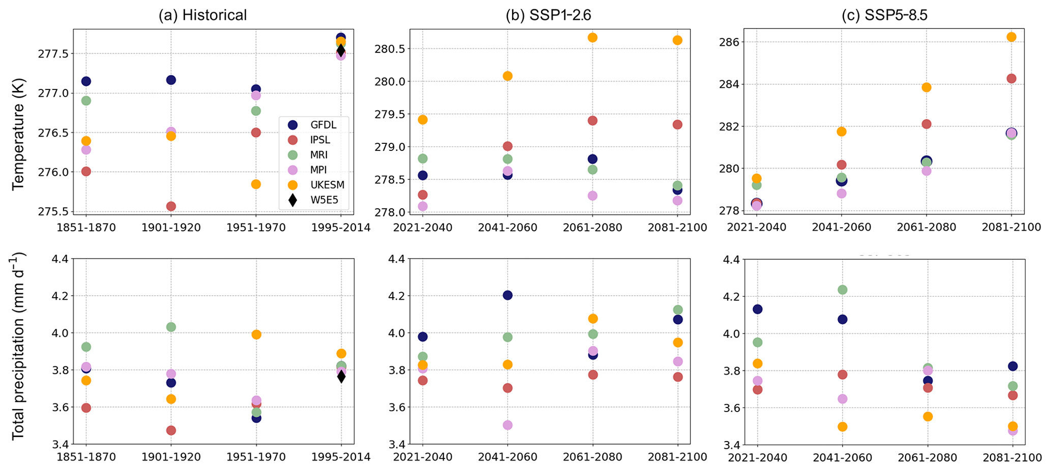
Figure 8 Temperature (K) and precipitation (mm d⁻¹) magnitudes in five CMIP6 models averaged over the glaciated grid cells in the Alps for the (a) historical, (b) SSP1-2.6, and (c) SSP5-8.5 scenarios. These are 20-year averages for the periods shown on the x axis.

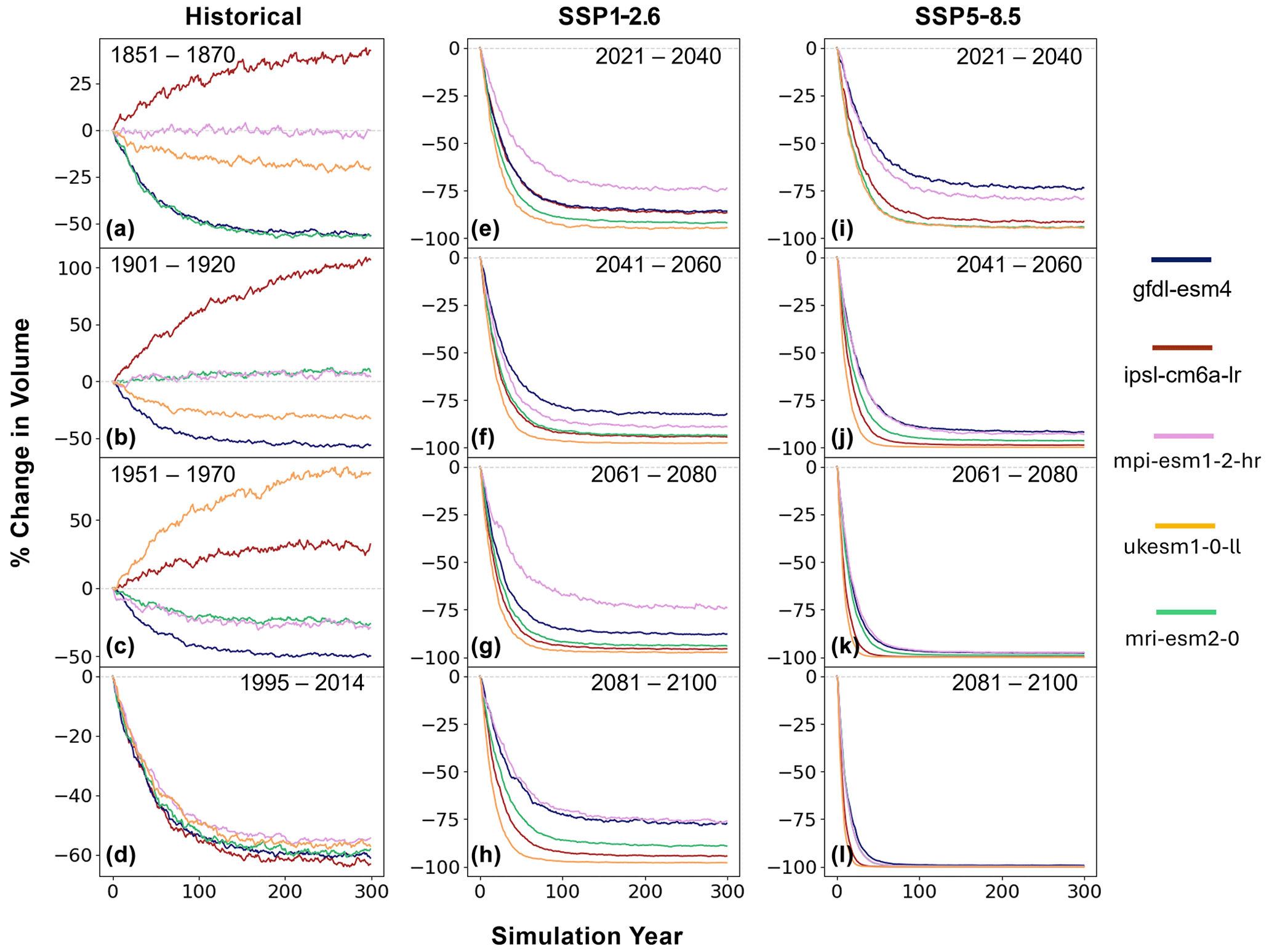
Figure 9 CISM–GlacierMIP3 experiment results, showing the percentage change in total ice volume in the Alps, for the climate periods and scenarios in Fig. 8. The x axis shows the first 300 simulation years of the 2000-year model run.

For 2021–2040 forcing under SSP5-8.5, the domain-mean annual temperature ranges from 278.2 K (MPI) to 279.5 K (UKESM) (Fig. 8c), and the total volume loss ranges from 73 % (GFDL) to 95 % (MRI and UKESM) (Fig. 9i). In comparison to the other models, the GFDL forcing drives less volume loss due to the higher precipitation and lower temperature (Fig. 8c). With slower warming, there is an increased response time; the time to equilibrium is about 140 years for GFDL, compared to 130, 100, and 90 years for MPI, IPSL, and UKESM/MRI, respectively; Fig. 9i).

In the projected climate of the later decades of SSP5-8.5, CISM predicts a near-complete loss of area and volume for all five models, with an equilibrium response time of less than 50 years (Fig. 9k, l). For the SSP1-2.6 scenario in the later decades, MPI and GFDL show less volume loss (about 75 %; Fig. 9h), noting that these models simulate slightly cooler temperatures than the other models (Fig. 8b).

We refer the reader to Zekollari et al. (2025) for a detailed analysis of GlacierMIP3 simulations by all participating models.

6 Computational performance

Three-dimensional glacier models are computationally more expensive compared to their 2D counterparts, limiting their ability to model large glaciated regions at high spatial resolutions on century-to-millennial scales. A 2-fold reduction in grid spacing quadruples the number of grid cells and typically halves the maximum stable time step, increasing the overall computational cost by a factor of 8. This suggests that the cost of glacier simulations using sub-kilometer grids would be several orders of magnitude higher than that of ice sheet simulations (generally run at 4 km resolution with CISM). However, we have implemented computationally efficient schemes in CISM to make glacier runs more affordable.

6.1 Spatial resolution and computational efficiency

For the Alps domain (Fig. 1), we created grids at 100 and 200 m resolutions to evaluate the sensitivity of model results and computational costs. On the 200 m grid, with the same model settings, we spun up the model for 7000 years, including 6000 years with inversion until the rate of volume change fell below 0.1 km³ per 1000 years. The final spun-up area and volume are 2530.8 km² and 137.9 km³, respectively, only slightly higher than the 100 m values (Table 2). In a commitment run (Sect. 5.1), the volume drops to 128 km³ (2003), 105 (2021), 65 (2084), and 53 (2184). The close similarity to the 100 m results suggests that the 200 m grid is adequate for regional-scale area and volume projections, although it fails to resolve many small glaciers. While 259 glaciers are unresolved on the 200 m grid, the 100 m grid resolves all but 6.

The 100 m grid has dimensions of 9611×5545 (more than 50 million grid cells), of which only about 250 000 are glaciated. To conserve computing resources, we created a glacier mask to identify regions that are currently ice-covered or could potentially contain ice if glaciers advance. The mask starts with ice-filled grid cells from the RGI input grid and is extended to a radius of 1 km around each glaciated cell. On initialization, CISM partitions the global domain into square blocks of data. For the 100 m grid, the initial domain consists of about 9300 blocks, each with 75 or 76 cells on a side. Of these blocks, only about 900 contain one or more of the grid cells included in the glacier mask. CISM labels these blocks as active, assigns one block to each processor core, and discards the remaining blocks. We modified CISM's parallel routines (halo updates, gather/scatters, global sums, and broadcasts) to operate only on active blocks, exchanging data with adjacent blocks that are also active. This allows a 10-fold reduction in cost compared to a simulation with inactive blocks included.

The atmospheric forcing consists of monthly mean temperature and precipitation. We found that runs on both grids were stable with a time step of 1 month (with each month containing exactly 30 d). This is similar to the maximum stable time step for CISM ice sheet simulations on a 4 km grid. Ice sheets require shorter time steps relative to the grid spacing because the fastest outlet glaciers have speeds of several kilometers per year. In the Alps, the maximum glacier speeds are only several hundred meters per year (Fig. 5; Millan et al., 2022).

6.2 High-performance computing costs

On the 100 m grid with a time step of 1 month, we achieved throughput of 145 model years per wall-clock hour on 896 processor cores (7 nodes with 128 cores each) on Derecho, a high-performance computing system at the NSF National Center for Atmospheric Research. The cost per simulated year is about 6.2 cpu hours. These numbers are for the last 1000 years of the spin-up; the throughput is ∼ 20 % lower during the first few model centuries. On the 200 m grid with the same time step but about 4 times fewer grid cells, the throughput is 588 model years per wall-clock hour on 768 cores, a cost of about 1.3 cpu hours per simulated year. Thus, the cost per cpu hour on the 100 m grid is about 4.8 times the cost on the 200 m grid, showing that the scaling is close to linear. The cost of the full spin-up on the fine grid is less than 4 times the cost on the coarser grid, since the model equilibrates in fewer years on the fine grid (Sect. 6.1).

These numbers suggest that applying CISM to regions larger than the Alps is computationally practical, especially with a resolution of 200 m. The four largest RGI regions (Alaska, Arctic Canada North, the Greenland periphery, and Antarctic islands) have a glaciated area of ∼10⁵ km² each. At 200 m resolution, this would imply 2.5 million glaciated cells per region. Assuming 10 ice-free grid cells per glaciated cell (i.e., somewhat denser glaciation than the Alps, where we have about 20 ice-free cells per glaciated cell), the computational domain would contain 25 million cells, or about 5 times as many as on the 100 m Alps grid. While substantial, the increased computational cost would not be prohibitive.

7 Model limitations and future work

7.1 SMB scheme

A limitation in the current modeling framework is the surface-mass-balance scheme, which is based on a temperature-index approach with a single glacier-specific degree-day factor μ. We adopted this approach for its simplicity and to make best use of the available datasets while accounting for their limitations.

For many glaciers, especially large ones, it is unrealistic to assume that a single degree-day factor applies to the entire glacier. The accumulation–ablation rates depend on terrain characteristics, microclimate effects, debris cover (Rounce et al., 2021), avalanches, and wind drift, among other factors. We refer the reader to Schuster et al. (2023) for a comprehensive assessment on the effects of SMB schemes, calibration approaches, and parameter values (e.g., lapse rate) on the accuracy of glacier projections.

We illustrate some limitations of the current SMB scheme by considering the Glacier du Tour, in the northwest part of the Mont Blanc massif. Figure 10a shows the thickness difference between the CISM spin-up and the F19 thickness estimates. This glacier has a tributary that lies between 2800 and 2900 m (dark purple shade in Fig. 10a), just above the equilibrium-line altitude (ELA). CISM, however, balances the glacier-wide SMB by choosing a value of μ that puts the ELA at around 2900 m, above the tributary. As a result, this region has a negative SMB, and since it is not fed by any ice in the accumulation zone, it remains ice-free. CISM's SMB scheme cannot account for ELA variations due to aspect and shading. This tributary has a north-facing aspect, ranging from northeast to northwest, and is shaded by steep ridges to the southwest (Fig. 10b, c), which could explain why its ELA, in reality, lies below the glacier mean ELA.

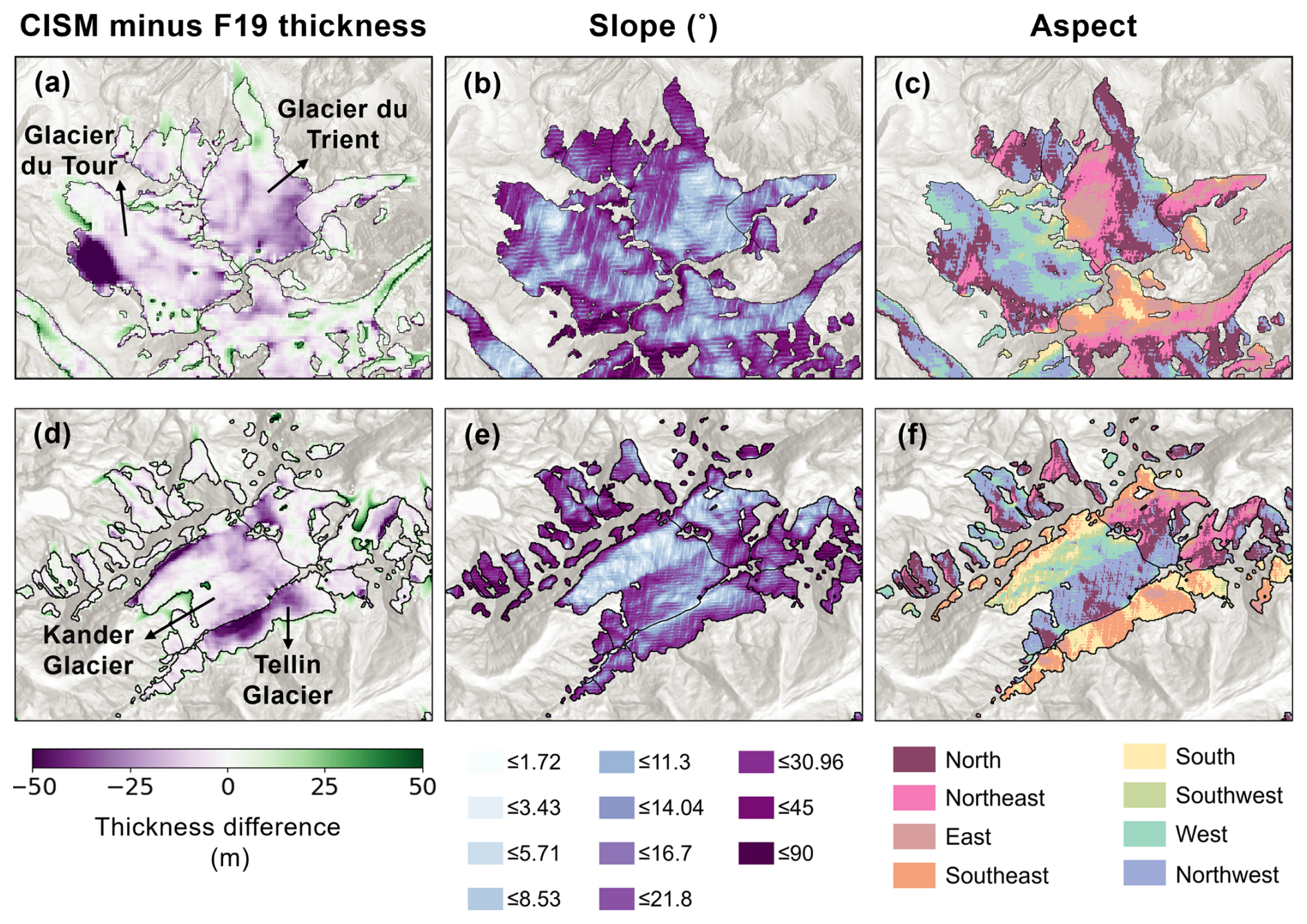
Figure 10 (a, d) Difference between 2003 CISM-simulated and F19 thickness (m) for select glaciers in the Mont Blanc massif (a) and the Bernese Alps (d). (b, e) Glacier slope and (c, f) aspect, from the surface elevation DEM, in the Mont Blanc massif (b, c) and the Bernese Alps (e, f).

Some of the differences between CISM and F19, however, stem from factors beyond the model's SMB limitations. Consider the Kander and Tellin glaciers in the western part of the Bernese Alps (Fig. 10d–f). Both glaciers have areas where the simulated ice in CISM is much thinner than the F19 estimates. These areas have steep slopes with a south and southeast aspect (Fig. 10e, f), leading to fast downhill flow that would tend to thin the ice at higher elevations. Faster downslope flow in CISM relative to the F19 models could explain the thickness differences. Running CISM forward to 2018 in a warming climate, we can compare model thicknesses with the observations from Grab et al. (2021). CISM agrees fairly well with the Grab et al. (2021) data (Fig. 3), which suggests that the model flow is realistic, perhaps more so than the F19 estimates. Hence, while certain differences between CISM and F19 are attributable to the limitations within CISM, other inconsistencies may be due to limitations in F19 or in both estimates.

To better capture topographic effects in future work, we plan to introduce a new SMB scheme within the land component of CESM, the Community Terrestrial Systems Model (CTSM; Lawrence et al., 2019), which computes surface mass balance using an energy-based scheme. With the hillslope hydrology configuration of CTSM (Swenson et al., 2019), we can account for aspect, relief, and slope and assess spatial variability in snow cover, debris cover, and local climate factors. CISM–CTSM coupling is currently limited to ice sheets, but we plan to add glacier coupling in future CESM versions, with the aim to improve SMB estimates.

7.2 Glacier initialization

CISM uses a simple, computationally efficient inverse method to estimate the spatial distribution of the basal friction coefficient C_p, adjusting the values to minimize the mismatch between modeled and observed ice thickness (Sect. 4.2). It is similar to the method developed by Pollard and DeConto (2012) to derive basal sliding coefficients for Antarctica. Other studies have used more sophisticated approaches such as adjoint-based optimization methods, which compute gradients of a cost function (typically the mismatch between modeled and observed velocities) with respect to control parameters using the adjoint of the governing equations, or transient (time-evolving) inversion, which assimilates time series of observations (Morlighem et al., 2013; Goldberg and Heimbach, 2013; Perego et al., 2014). At present, CISM does not have these capabilities for ice-flow modeling.

7.3 Uncertainty in atmospheric forcing

High-resolution, high-fidelity land and glacier models often require better-resolved, higher-quality forcing data than their simpler counterparts; otherwise their accuracy is often constrained by the lower resolution of atmospheric data. For example, Gabbi et al. (2014) found that a full energy-balance model is less consistent with observations than simpler models, despite being able to capture relevant physical processes in detail. The energy-balance model is more sensitive than simpler models to errors in the atmospheric forcing. Nevertheless, improvements in satellite data and the application of machine learning to data assimilation are gradually resolving these issues; these advancements will guide future CISM developments.

7.4 Missing processes

This initial implementation applies to land-terminating glaciers only, whereas many RGI regions (including Alaska, Arctic Canada, Svalbard, the Russian Arctic, the Greenland periphery, and Antarctic islands) have glaciers that flow into the ocean. In other regions, such as High Mountain Asia and Patagonia, many glaciers terminate in lakes. While CISM includes subgrid parameterizations for iceberg calving and grounding-line migration in ice sheets (Lipscomb et al., 2019; Leguy et al., 2021), we have not yet implemented these processes for mountain glaciers. This will require a glacier calving parameterization, along with a modified SMB calibration scheme that accounts for the additional mass loss. Finally, CISM currently does not account for glacier surges, which would require a more sophisticated treatment of subglacial hydrology. This is left for future work.

8 Conclusions

We have implemented a new framework for modeling mountain glaciers using the Community Ice Sheet Model, which was originally developed to study ice sheets. We used this framework to study the evolution of the nearly 4000 glaciers of the European Alps. This is one of the first uses of a 3D, higher-order ice-flow model to simulate thousands of glaciers at the scale of an RGI region. Unlike traditional flowline models, a 3D, higher-order model can resolve complex topography and ice-flow patterns, simulating horizontal and vertical variations in velocity, temperature, and stress, thus providing more detailed glacier predictions in complex terrain.

We initialized the model on a 100 m grid to a stable state using 1980s atmospheric data, a period when we assumed the Alpine glaciers to be in near equilibrium with the climate. During the spin-up, we calibrated surface-mass-balance and basal friction parameters to optimize agreement with observation-based area and thickness targets. We then ran the model forward to the present, simulating glacier retreat in a warming climate. We obtained strong agreement with the consensus ice thickness estimates and satellite-observed ice velocities. Using the GlacierMIP3 protocols, we ran the model to equilibrium under various forcing scenarios corresponding to five different CMIP6 Earth system models, several historical and future periods, and three emissions scenarios. With present-day climate forcing (2000–2019), we found that the glaciers of the Alps are committed to losing more than half their area and volume relative to the present day. We simulated near-total ice loss in warmer climate scenarios, with most of the loss taking place before 2100. Climate sensitivity for the Alps in CISM is similar to that of other GlacierMIP3 models analyzed by Zekollari et al. (2025).

We have shown that large-scale, high-resolution, decade-to-millennial-scale glacier simulations can be run at reasonable cost on high-performance computers, due to CISM's parallel scalability, efficient higher-order velocity solver, and methods for limiting the computational domain to active glacier regions. Similar simulations for larger RGI regions should be computationally feasible and would enable further assessments of the sensitivity of glacier projections to model complexity. Comparing multiple models of varying complexity will enhance our understanding of glacier systems.

This work suggests many possible areas for improvement: for example, (1) using the Community Terrestrial Systems Model within the CESM framework to improve SMB calculations by adding physical factors and terrain characteristics such as aspect, slope, and debris cover; (2) extending the model to lake-/marine-terminating glaciers, which would require a treatment of calving; (3) modeling glacier surges, which demands more sophisticated subglacial hydrology; and (4) introducing more rigorous model initialization techniques.

Overall, these simulations are a step towards unification of glacier and ice sheet studies in a common modeling framework. This model development will enable assessments of interactions and feedback mechanisms between land ice and connected processes including freshwater resources, ecosystem dynamics, and sea-level rise using CESM.