the Creative Commons Attribution 4.0 License.
the Creative Commons Attribution 4.0 License.
 | 26 Aug 2025
A regional physical–biogeochemical ocean model for marine resource applications in the Northeast Pacific (MOM6-COBALT-NEP10k v1.0)
Elizabeth J. Drenkard
Charles A. Stock
Andrew C. Ross
Yi-Cheng Teng
Theresa Cordero
Wei Cheng
Alistair Adcroft
Enrique Curchitser
Raphael Dussin
Robert Hallberg
Claudine Hauri
Katherine Hedstrom
Albert Hermann
Michael G. Jacox
Kelly A. Kearney
Rémi Pagès
Darren J. Pilcher
Mercedes Pozo Buil
Vivek Seelanki
Niki Zadeh
Regional ocean models enable the generation of computationally affordable and regionally tailored ensembles of near-term forecasts and long-term projections of sufficient resolution to serve marine resource management. Climate change, however, has created marine resource challenges, such as shifting stock distributions, that cut across domestic and international management boundaries and have pushed regional modeling efforts toward “coastwide” approaches. Here, we present and evaluate a multidecadal hindcast with a Northeast Pacific regional implementation of the Modular Ocean Model, version 6, with sea ice and biogeochemistry that extends from the Chukchi Sea to the Baja California Peninsula at 10 km horizontal resolution (MOM6-COBALT-NEP10k, or NEP10k). This domain includes an Arctic-adjacent system with a broad, shallow shelf seasonally covered by sea ice (the eastern Bering Sea), a sub-Arctic system with upwelling in the Alaska Gyre and predominant downwelling winds and large freshwater forcing along the coast (the Gulf of Alaska), and a temperate, eastern boundary upwelling ecosystem (the California Current Ecosystem). The coastwide model was able to recreate seasonal and cross-ecosystem contrasts in numerous ecosystem-critical properties including temperature, salinity, inorganic nutrients, oxygen, carbonate saturation states, and chlorophyll. Spatial consistency between modeled quantities and observations generally extended to plankton ecosystems, though small to moderate biases were also apparent. Fidelity with observed zooplankton biomass, for example, was limited to first-order seasonal and cross-system contrasts. Temporally, simulated monthly surface and bottom temperature anomalies in coastal regions (<500 m deep) closely matched estimates from data-assimilative ocean reanalyses. Performance, however, was reduced in some nearshore regions coarsely resolved by the model's 10 km resolution grid and for point measurements. The time series of satellite-based chlorophyll anomaly estimates proved more difficult to match than temperature. System-specific ecosystem indicators were also assessed. In the eastern Bering Sea, NEP10k robustly matched observed variations, including recent large declines, in the area of the summer bottom water “cold pool” (<2 °C), which exerts a profound influence on eastern Bering Sea fisheries. In the Gulf of Alaska, the simulation captured patterns of sea surface height variability and variations in thermal, oxygen, and acidification risk associated with local modes of interannual to decadal climate variability. In the California Current Ecosystem, the simulation robustly captured variations in upwelling indices and coastal water masses, though discrepancies in the latter were evident in the Southern California Bight. Enhanced model resolution may reduce such discrepancies, but any benefits must be carefully weighed against computational costs given the intended use of this system for ensemble predictions and projections. Meanwhile, the demonstrated NEP10k skill level herein, particularly in recreating cross-ecosystem contrasts and the time variation of ecosystem indicators over multiple decades, suggests considerable immediate utility for coastwide retrospective and predictive applications.
- Article
(30468 KB) - Full-text XML
-
Supplement
(14221 KB) - BibTeX
- EndNote


The western coasts of the continental United States, Canada, and Mexico form the eastern bounds of the North Pacific Gyre, which substantially impacts North American climate and supports a diverse assemblage of ecosystems, species, and resources. These ecosystems include valuable fisheries that represented roughly 42 % of the USD 4.6 billion in commercial U.S. domestic landings in 2020 (National Marine Fisheries Service, 2022). Management of these interconnected, multiscale marine resources presents a challenge, particularly with the growing need to account for changing climate and ocean conditions. Ocean warming, acidification, and deoxygenation stand to fundamentally alter coastal ecosystems (Gruber, 2011), potentially driving fluctuations in living marine resource abundance due to habitat range shifts (e.g., Pinsky et al., 2013; Christian and Holmes, 2016; Smith et al., 2021; Chasco et al., 2022; Thompson et al., 2023), recruitment and fish size changes (e.g., Holsman et al., 2019; Litzow et al., 2022), and heightened competition and predation from invasive species (Grosholz et al., 2000; Zeidberg and Robison, 2007; Compton et al., 2010). Additionally, extreme events such as marine heat waves (e.g., Rogers-Bennett and Catton, 2019; McPherson et al., 2021) and harmful algal blooms (e.g., Anderson et al., 2015) can degrade foundational habitats and compromise water quality.
Numerical ocean models facilitate both the understanding of difficult-to-observe ocean and ecosystem dynamics and the forecasting and projection of near- to long-term ocean conditions. Previous regional modeling efforts in the Northeast Pacific Ocean have contributed considerably to our understanding of the Bering Sea (Danielson et al., 2011; Hermann et al., 2013, 2016; Cheng et al., 2015; Pilcher et al., 2019; Kearney et al., 2020), Gulf of Alaska (Hermann et al., 2009; Hinckley et al., 2009; Cheng et al., 2012; Coyle et al., 2012, 2019; Danielson et al., 2020; Hauri et al., 2020, 2024), and California Current System (Marchesiello et al., 2001; Di Lorenzo et al., 2005; Gruber et al., 2006; Veneziani et al., 2009; Neveu et al., 2016; Van Oostende et al., 2018; Dussin et al., 2019; Deutsch et al., 2021; Renault et al., 2021) and the broader NEP10k domain (Desmet et al., 2022, 2023). Predictions and projections from these regionally tailored ocean models have also been enlisted to understand and anticipate living marine resource responses to climate variability and change (e.g., Gruber et al., 2012; Hermann et al., 2016; Holsman et al., 2020; Siedlecki et al., 2016; Howard et al., 2020; Pozo Buil et al., 2021; Pilcher et al., 2022; Jacox et al., 2023). In a growing number of cases, applications have been extended to management (e.g., Anderson et al., 2016; Punt et al., 2021; Brodie et al., 2023; Smith et al., 2023; Hollowed et al., 2024). Such applications have been hampered, however, by the use of relatively small domains and limited ensembles to characterize uncertainties. Climate change impacts and species responses traverse the bounds of those domains, thus motivating an integrated “coastwide” modeling framework with rigorously defined uncertainties.
A key challenge is thus configuring a coastwide modeling framework with sufficient resolution and complexity to adequately represent fisheries-critical ocean features across the full domain while also maintaining low computational cost conducive to generating ensembles (Drenkard et al., 2021). This challenge is made more acute by the diversity of Northeast Pacific ecosystems and the mechanisms by which climate shapes them. The Bering Sea, for example, features one of the world's broadest shallow continental shelf environments, which supports benthic and demersal fisheries that are amongst the most productive in the world (National Research Council, 1996). These fisheries, however, have proven to be highly sensitive to temperature and food fluctuations in these shallow habitats (Hunt et al., 2002, 2011). Recent warming and reduced food supply in the eastern Bering Sea (EBS), for example, was linked to the collapse of the snow crab fishery (Szuwalski et al., 2023). Productivity as well as benthic and pelagic habitat fluctuations on the eastern Bering shelf are further linked to coupled ocean and sea ice dynamics (Mueter and Litzow, 2008; Brown and Arrigo, 2013; Hunt et al., 2022), presenting an additional challenge for ocean modeling systems intended for fisheries applications in this region.
In the Gulf of Alaska (GOA), downwelling winds and abundant freshwater input prevail and contribute to a strong cyclonic circulation of the Alaska Gyre (Stabeno et al., 2004). Despite the predominance of downwelling winds, the confluence of the high nitrate waters of the basin with the high iron waters of the shelf (assisted by shelf-break eddies), as well as upwelling of nitrate by wind stress curl, promote high production in the coastal GOA (Stabeno et al., 2004; Hermann et al., 2009; Coyle et al., 2019). While correlation with the El Niño–Southern Oscillation (ENSO) can be found (e.g., Bailey et al., 1995; Whitney and Welch, 2002; Amaya et al., 2023b), lower-frequency modes of decadal climate variability tend to predominate (e.g., Di Lorenzo et al., 2008) and are associated with marked decadal-scale ecosystem regime shifts (Anderson and Piatt, 1999; Hare and Mantua, 2000) and modulations in fisheries and ecosystem risks (Hauri et al., 2021, 2024). Cold water temperatures and the proximity of North Pacific basin waters, which are exceptionally rich in dissolved inorganic carbon (DIC), make the Gulf of Alaska particularly susceptible to ocean acidification (Fabry et al., 2009; Byrne et al., 2010; Mathis et al., 2015). Periodic on-shelf intrusions of DIC-rich deep Pacific water can suppress the aragonite and calcite saturation states and stress commercially important crab and shell fisheries (Ladd et al., 2005). Increased freshwater input due to deglaciation, which is naturally low in alkalinity, may also exacerbate coastal acidification trends (Reisdorph and Mathis, 2014; Evans et al., 2014). In offshore waters, the iron supply strongly modulates ocean productivity, though the impacts of such variations on fisheries remains speculative (Lippiatt et al., 2010; McKinnell, 2013; Kearney et al., 2015).
The California Current is one of the four major eastern boundary upwelling systems in the global ocean (Hill et al., 1998). Marine resource fluctuations are inextricably linked to variations in the timing, strength, and source waters of this seasonal upwelling (e.g., Bograd et al., 2009). Physical, biogeochemical, and marine resource dynamics of the California Current correspond strongly with ENSO (Ohman et al., 2017; Turi et al., 2018; Cordero-Quirós et al., 2022) through diverse atmospheric and oceanic teleconnection pathways (Alexander et al., 2002; Jacox et al., 2015; Frischknecht et al., 2015). While a narrow shelf and modest riverine inputs over much of the coast give the California Current an oceanic character, the system nonetheless supports significant benthic and demersal fisheries, which are periodically subject to heightened hypoxia and acidification risks common in upwelling systems (Bograd et al., 2008; Hauri et al., 2009; Wolfe et al., 2023). These risks can be further amplified by processes resulting from changing land use such as increased nutrient input, pollution, and coastal engineering (e.g., Halpern et al., 2009; Hughes et al., 2015). The considerable productivity generated by coastal upwelling also supports climate-sensitive forage fish, highly migratory species, and top predators that are ecologically, economically, and culturally important. Projections suggest that upwelling strength, seasonality, and source water properties may shift with climate change (Rykaczewski and Dunne, 2010; Rykaczewski et al., 2015; Sydeman et al., 2011; Pozo Buil et al., 2021) and significantly alter ecosystem productivity and fisheries (McClatchie et al., 2010; Bograd et al., 2023; Jacox et al., 2024).
Here, we present a regional implementation of the modular ocean model (MOM6) with coupled sea ice and biogeochemistry spanning the Northeast Pacific and assess the degree to which this system can capture fisheries-critical mean patterns and fluctuations across the diverse ecosystems of the Northeast Pacific. We evaluate the model's capacity to represent both large-scale contrasts in ecologically important variables across ecosystems and variations in fisheries-oriented diagnostics within each ecosystem. We also assess computational costs to ensure the feasibility of ensemble predictions. We conclude with an assessment of the model's current utility for fisheries applications and a discussion of priority developments for addressing model biases in order to maximize future utility in informing fisheries and ecosystem decisions.
2.1 Physical model configuration
The NEP10k model domain (Fig. 1) is designed to cover the western coast of the continental United States and contiguous regions. It extends from 10.8–80.7° N and 156.6° E–105.0° W, measuring 3320 ± 126 km by 7764 ± 58 km (mean ± standard deviation) in the offshore and along-shore dimensions, respectively. The model is integrated on an orthogonal curvilinear grid that consists of 342×816 tracer cells with a horizontal resolution averaging 9.7 ± 0.5 km and a minimum bathymetric depth of 10 m. The domain has four open boundaries, the longest of which arcs through the Pacific Ocean and is referenced as the “western” boundary. In the vertical direction, the model uses 75 z* coordinates, which are approximately consistent with the depth-from-mean-sea-level but are stretched by variations in sea surface height across all water column layer thicknesses rather than isolating that variability in the surface layer (Adcroft and Campin, 2004). We prescribe a layer thickness of 2 m from the surface to a depth of 8 m, between 2.01 to 2.34 m in thickness between 8 and ∼31 m in depth, then with spacing gradually increasing to 250 m in the deepest portions of the model domain. Bathymetry for the NEP10k domain was derived from the 2020 General Bathymetric Chart of the Oceans (GEBCO Bathymetric Compilation Group, 2020) and is not vertically rounded or truncated. MOM6 does not need the topography to conform to the vertical level thicknesses but instead can let the bottommost non-vanished layer vary in thickness to match the topography and then collapse the layer to zero thickness below where the topography intersects the model layer. Simulations used a baroclinic time step of 400 s and a variable barotropic time step set to maintain stability (Hallberg, 1997; Hallberg and Adcroft, 2009). A longer, 1200 s time step was used for thermodynamic and biogeochemical tracer calculations, as thermodynamic processes tend to evolve more slowly than dynamic ones. Past studies have used a longer time step for these processes without compromising their representation while reducing the overall computation time (e.g., Ross et al., 2023). The success of this strategy for the NEP10k domain will be assessed herein.
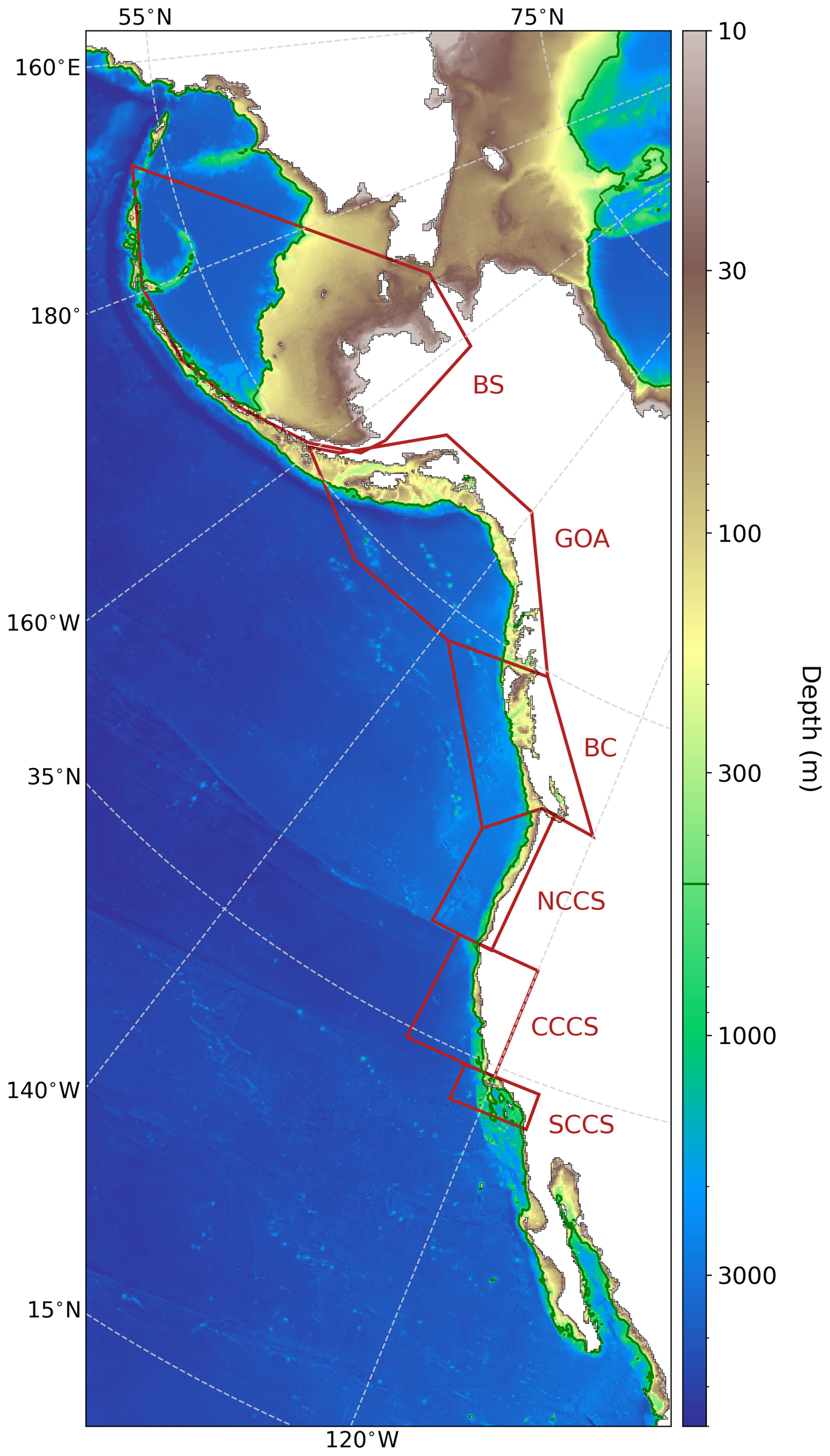
Figure 1NEP10k domain and bathymetry. NEP10k domain and bathymetry with a log-normal color scale to emphasize priority coastal regions. White coloration indicates non-ocean (i.e., land-masked) grid cells that are not computed in model integrations, which include the Sea of Okhotsk. The agglomerate land mask is outlined in black. Red lines indicate the areas that are spatially averaged for regional shelf temperature and chlorophyll time series. These regions, from north to south, are the Bering Sea (BS), Gulf of Alaska (GOA), British Columbia (BC), Northern California Current System (NCCS), Central California Current System (CCCS), and Southern California Current System (SCCS). The southern arc of the Bering Sea polygon traces the Aleutian island chain; the southernmost land bounds of the Southern California Current System and Gulf of Alaska polygons, as well as both the northernmost and southernmost land bounds of the British Columbia polygons, roughly correspond with international geopolitical boundaries. The dark green contour delineates the 500 m isobath, which we use to isolate shelf grid cells (i.e., where depth ≤500 m).
The core components of the physical ocean model, Modular Ocean Model 6 (MOM6), are described in Adcroft et al. (2019). A full account of the parameterization choices implemented for the simulations presented in this study can be found in the Supplement in Drenkard et al. (2024a) (MOM_parameter_doc.all). Here, we elaborate on a few choices (Table A1), highlighting consistencies and contrasts with the recently published Northwest Atlantic configuration documented in Ross et al. (2023). As in Ross et al. (2023), ocean boundary layer mixing, specifically vertical turbulent mixing coefficients in the surface layer, are parameterized using the energetic planetary boundary layer (ePBL) scheme developed by Reichl and Hallberg (2018). However, unlike Ross et al. (2023), we switched to the submesoscale mixing and restratification scheme of Bodner et al. (2023) from that of Fox-Kemper et al. (2011). The Bodner parameterization has the advantage of dynamically calculating the submesoscale front length (i.e., the length scale perpendicular to the front), which can vary significantly seasonally and latitudinally across the ecosystems represented in NEP10k (Bodner et al., 2023). In the ocean interior below the surface boundary layer, mixing primarily depends on the shear-driven turbulence mixing scheme of Jackson et al. (2008). The standard Jackson formulation, however, was found to overmix some shelf regions subject to strong tidal motions. This overmixing was ameliorated by including a scaling factor for the turbulent decay length scale. Bottom drag and horizontal viscosities were parameterized as in Ross et al. (2023). Unlike Ross et al. (2023), the background kinematic viscosity parameter, KV, was set to 0.0 m2 s−1; this parameter is intended to supplement the existing dynamic viscosity (based on the diapycnal diffusivity, KD) and was determined to be unnecessary for this application. Sea ice is modeled with the Sea Ice Simulator, version 2 (SIS2, Adcroft et al., 2019). This sea ice model uses five sea ice thickness categories and no explicit ridging scheme. The sea ice rheology is an elastic-viscous-plastic scheme (Hibler, 1979) and a directionally split piecewise constant advection scheme for thickness. The delta-Eddington radiation scheme is used, and the internal thermodynamics are enthalpy-conserving (Briegleb and Light, 2007).
2.2 Physical model forcing
The ocean hindcast simulation was run from 1993 through 2019 on NOAA's GAEA supercomputer, which is housed and managed in partnership with the Department of Energy through the National Climate-Computing Research Center. Hourly atmospheric forcing for NEP10k was prescribed from the European Centre for Medium-Range Weather Forecasts Reanalysis 5 (ERA5; Hersbach et al., 2020). The bulk formulae of Large and Yeager (2004) were used to calculate latent and sensible heating after adjusting to the 2 m ERA5 reference height. Light attenuation and associated heating within the water column was calculated from Manizza et al. (2005) using dynamically varying chlorophyll from the biogeochemical model (Sect. 2.3).
Daily freshwater runoff was prescribed using output from the Global Flood Awareness System, version 4.0 (GloFAS; Harrigan et al., 2020; Grimaldi et al., 2022) – a hydrological inundation model that is also forced by ERA5. Freshwater discharge at ocean-adjacent “pit cells” in GloFAS was remapped to the nearest MOM6 coastal ocean grid cells. Pit cells are GloFAS grid cells where the local drain direction indicates that only inward water flow occurs and is therefore a point of accumulation (e.g., lakes) or a point of egress to the ocean via either ocean adjacency or connectivity through other pit cells (e.g., wetlands). For the Gulf of Alaska, we substituted freshwater discharge from Beamer et al. (2016; Hill, 2023), a model dedicated to the representation of freshwater discharge and glacier mass balance in Alaska, with calibration against observed watersheds.
Open lateral boundary and initial conditions for temperature, salinity, sea surface height, and momentum were prescribed as daily means from the ° Global Ocean Physics Reanalysis (GLORYS12; Lellouche et al., 2021). Tidal forcing was prescribed at the boundaries using the amplitude and phase from the global tidal elevation and transport atlas, version 9 (TPXO; Egbert and Erofeeva, 2002). Tides were implemented as in Ross et al. (2023) with four semidiurnal constituents (M2, S2, N2, K2), four diurnal constituents (K1, O1, P1, Q1), and two long-period constituents (Mm and Mf). Initial and boundary conditions were regridded to the NEP10k domain using the xESMF Python software package (Zhuang et al., 2023). Boundary conditions were imposed as in Ross et al. (2023), with barotropic flows handled with a Flather (1976) boundary condition, while baroclinic flows are handled with an Orlanski (1976) radiation condition. Lateral boundary forcing also applies nudging and tracer reservoirs (the latter retains a memory of water properties exchanged with the modeling domain rather than instantaneous forcing; see Ross et al., 2023, for more details). As in Ross et al. (2023), the lateral ocean boundary radiation and nudging schemes utilize 3 d inflow, 360 d outflow timescales, and both inward and outward tracer reservoir length scales were 9000 m (Table A1). No nudging was included in the interior of the domain.
2.3 Biogeochemical model configuration
Biogeochemistry was simulated using version 3.0 of the Carbon, Ocean Biogeochemistry, and Lower Trophics (COBALTv3.0) model (Stock et al., 2025; Ross et al., 2023). COBALTv3.0 includes 40 prognostic state variables to capture plankton food web dynamics and the cycling of carbon, nitrogen, phosphorus, iron, silica, calcium carbonate, and lithogenic material in ocean and coastal environments. COBALTv3.0 builds on prior COBALT formulations (Stock et al., 2014, 2020) by adding a third phytoplankton size class following Van Oostende et al. (2018). The resulting small, medium, and large sizes correspond to the canonical pico-, nano-, and microplankton size classes defined by Sieburth et al. (1978) and enable COBALT to better resolve the range of phytoplankton communities from oligotrophic gyres to intensely productive upwelling systems. These join diazotrophs to give a total of four phytoplankton functional types to go along with a plankton food web including three zooplankton functional types and free living bacteria (Stock et al., 2014, 2020). Additional flexibility in zooplankton feeding, direct phytoplankton sinking, and improved photoadaptation and photoacclimation dynamics were also added (Stock et al., 2025), and the formulation enlists an adaptation of the dynamic N:P ratio scheme proposed by Galbraith and Martiny (2015) and initially presented in Ross et al. (2023).
Initial and boundary conditions for biogeochemistry were drawn from the same sources as Ross et al. (2023). The 2018 World Ocean Atlas (WOA18) was used for macronutrients (NO3, PO4, SiO4) and oxygen (O2), with seasonal averages above 800 m and annual climatologies below (Boyer et al., 2019; García et al., 2019a, b). The Empirical Seawater Property Estimation Routines Locally Interpolated Regressions (ESPER_LIR) presented by Carter et al. (2021) were used to provide initial and time-varying (i.e., seasonal, interannual to decadal variability, and multidecadal trends) boundary conditions for dissolved inorganic carbon and alkalinity. The input values used for this calculation were the location, temperature, salinity, and date. Boundary conditions for other tracers, which generally come into more rapid equilibrium with interior conditions, were drawn from an earlier global ocean hindcast (Stock et al., 2014).
River carbon, alkalinity, nutrients (N, P, and Si) and oxygen inputs were derived by combining the River Chemistry for U.S. Coast (RC4USCoast) database (Gomez et al., 2023) for U.S. waters in the continental United States, the Global River Chemistry database (GLORICH, Hartmann et al., 2019, 2014) for subarctic/Canadian waters, and the Arctic Great Rivers Observatory (Holmes et al., 2012; ArcticGro, 2024). To force COBALT, riverine nutrient inputs are needed for dissolved inorganic and organic nitrogen and phosphorus, particulate nitrogen, phosphorus, and iron. Direct information on dissolved and particulate organic nutrient inputs was not available in all cases. In cases where one or both of these values were missing, the ratio of dissolved and/or particulate organic inputs to dissolved inorganic nitrogen was estimated from the Global Nutrient Export from WaterSheds (Global NEWS) model (Mayorga et al., 2010). This NEWS-derived ratio was then multiplied by the observed inorganic nitrogen to estimate dissolved and particulate organic fluxes in a manner that preserved their relative importance but avoided regional biases in global nutrient-load models such as Global NEWS. Dissolved organic nitrogen and phosphorus was partitioned into 40 % labile, 30 % semi-labile, and 30 % semi-refractory components in COBALT to be consistent with mean tendencies reported by Wiegner et al. (2006). Particulate phosphate is often the largest phosphorus source in rivers, but much of it is buried in nearshore waters before reaching the ocean. Following Froelich (1988), we assumed that 30 % of the particulate phosphorus was mobilized in estuarine sediments to phosphate, with the rest buried. Iron concentrations for all rivers were set to 70 nM (de Baar and de Jong, 2001). As in Ross et al. (2023), atmospheric CO2 was set using the monthly historical time series of Meinshausen et al. (2017), updated after 2014 using SSP2-4.5 scenario values (Meinshausen et al., 2020), and nutrient, dust, and iron deposition were based on a 1993–2014 climatology from GFDL's ESM4.1 model (Dunne et al., 2020; Stock et al., 2020).
2.4 Model spinup and simulation
Similar to Ross et al. (2023), we initialized the 1993–2019 hindcast simulation from rest starting at 1 January 1993, with ocean physics prescribed from GLORYS (described above), and we initialized the ocean biogeochemistry from a 10-year spinup simulation. We generated the spinup simulation by starting the model integration from rest on 1 January 1993 and by repeating ERA5 atmospheric conditions for 1993–1994 (May–December of 1993 and January–April 1994; following Stewart et al., 2020) for 10 1-year cycles. Atmospheric CO2 was maintained as the 12-month, 1993 seasonal climatology, and the ocean boundaries were forced with a smoothed, daily climatology (i.e., averaged by “day of year” and smoothed with a triangular filter) of the hindcast's GLORYS12 1993–2019 open boundary conditions. River runoff was similarly prescribed as a smoothed daily climatology. The biogeochemical tracer fields at the end of this 10-year spinup simulation were then used to initialize biogeochemistry for the 27-year hindcast simulation.
The purpose of implementing a spinup was to omit drifts in the biogeochemistry associated with the adjustment of the model from its initialized state, which was generally based on coarse-resolution observation-based products, to the model's characteristic solution. We focused on fisheries-relevant variables in the top 500 m. We found that a spinup period of 10 years generally resolved initial model adjustments, which were strongest in the British Columbia region (Fig. S3 in the Supplement). While 10 years removed the strongest drifts, subtle trends remain in some regions, suggesting the potential value of longer spinup periods, particularly for representing the deeper ocean. These spinup sensitivities are left to future NEP10k development efforts.
2.5 Model evaluation
As described in Sect. 1, the model evaluation focuses on the simulation's capacity to represent fisheries and ecosystem-relevant features across and within the diverse ecosystems included within the NEP10k domain. The model evaluation therefore includes comparisons against both large-scale physical and biogeochemical patterns spanning the full domain (Sect. 2.5.1) and ecosystem-specific quantities (Sect. 2.5.2). These latter quantities were often drawn from Ecosystem Status Reports developed by NOAA fisheries to strategically inform marine resource management decisions (e.g., Ferriss, 2023; Siddon, 2023; Leising et al., 2024). Comparisons against spatial and seasonal patterns were complemented with interannual time series comparisons where possible; the latter serves as a building block toward making predictive applications. We note that several comparisons are made against gridded data products that were also used to force and initialize the NEP10k hindcast (i.e., GLORYS, TPXO, WOA23). While these comparisons are not fully independent, they are nonetheless meaningful tests of the capacity of the regional model to translate horizontal boundary and surface forcing into an interior solution that remains consistent with observations. The regional model must explain multiple observed interior properties by dynamically extending from the specified boundaries with a single set of self-consistent explicitly specified dynamics without the benefit of assimilating, or being informed by, observation from within the domain. Maintaining agreement with observation-based products in the domain interior thus supports the fidelity of these dynamics. We lastly assess the computational performance and viability of the model using analyses described in Sect. 2.5.3.
2.5.1 Full domain comparisons
We broadly evaluated NEP10k performance against gridded surface and 3D observation-based or observation-assimilated physical and biogeochemical products to assess the simulation's coastwide capacity to represent cross-ecosystem patterns. Table A2 summarizes these products and the time frames analyzed. For spatial comparisons and calculations, we first plot both the NEP10k results and the comparison product on their native grids using the Python geographic plotting package Cartopy (Met Office, 2022). We then regridded the finer-resolution product output (typically NEP10k, but not in the case of comparisons against GLORYS12 and chlorophyll comparisons) to the coarser-resolution comparison grid using the Earth System Modeling Framework (Hill et al., 2004) Python Regridding Interface (ESMPy) or xESMF conservative regridding (Zhuang et al., 2023). Unless otherwise stated, assessments include the area-weighted spatial mean bias (Bias, NEP10k – comparison data product), area-weighted root mean squared error (RMSE), median absolute error (MedAE), and Pearson correlation coefficient (R, based on the spatial pattern). We omit analysis of model performance in the Chukchi Sea (i.e., north of the Bering Strait at 66° N) – this region is included in the model integration due to the rectilinear nature of the grid and our objective to include the entire Bering Sea for which the Chukchi provides a boundary condition. However, it is not a primary region of interest for this model application and will be assessed in a nascent pan-Arctic MOM6 configuration.
For ocean temperature validations, we compared conditions against version 2.1 of the Daily Optimum Interpolation Sea Surface Temperature product (OISSTv2.1; Huang et al., 2021) and against GLORYS12 for both surface and subsurface conditions. OISSTv2.1 is generated from multiple temperature data sources and interpolated to a ° global grid, whereas GLORYS12 is a global eddying (°) data-assimilative ocean reanalysis that demonstrates strong coherence with in situ surface and subsurface temperature records along the U.S. West Coast (Amaya et al., 2023a). Both reference products have a continuous monthly output covering 1993–2019.
NEP10k surface and subsurface salinity is compared against GLORYS12 reanalysis as well as the observation-based NOAA National Centers for Environmental Information (NCEI) ° Northern North Pacific (nnp; Version 2, Seidov et al., 2023) and Northeast Pacific (nep; Seidov et al., 2017) regional climatologies for salinity. Annual and seasonal means were downloaded for both nep and nnp regions for the decades 1995–2004 and 2005–2014 (the second decade for the older nep climatology only extends 2005–2012). To ensure temporal coherence, we regrid NEP10k separately for each region, using only the years represented by each regional climatology (i.e., 1995–2012 for the nep and 1995–2014 for the nnp). The two decadal, annual, and seasonal means for the regional climatologies are time-weight averaged, and then the regional climatologies and regridded NEP10k output are combined into a common grid. Where the nnp and nep regions overlap in the GOA (i.e., above 50° N), we use the values from the more recent nnp climatology.
We validated NEP10k mixed layer depth (MLD) against the 1° de Boyer Montégut (2024) monthly MLD climatology, which incorporates measurements from an assemblage of MBT, XBT, and CTD casts and profiling floats and defines the MLD as the seawater depth where the potential density is 0.03 (kg m3) greater than the density at a reference depth of 5 m. From NEP10k, we used the MOM6 diagnostic variable MLD_003, which calculates the mixed layer depth based on a user-defined reference depth (in our case, 5 m for consistency with de Boyer Montégut). The mixed layer depth is identified as the depth where the potential density increases by 0.03 kg m3 relative to the surface reference depth. We also compared NEP10k MLD against GLORYS12. The approximately equivalent MLD for GLORYS12 was determined by first calculating the potential density from monthly GLORYS12 potential temperature and salinity using the Python implementation of the Gibbs SeaWater (GSW) Oceanographic Toolbox of TEOS-10 (McDougall and Barker, 2011). We then calculated GLORYS12 MLD using the same criteria as de Boyer Montegut (2024) and the NEP10k MLD_003 diagnostic (i.e., depth at which potential density is 0.03 kg m3 greater than the density at 5 m depth at a given location).
NEP10k sea surface height (SSH) was compared against GLORYS12 sea surface height above geoid (zos) and absolute dynamic height (adt) above the Earth's geopotential surface (i.e., geoid) from 0.083° resolution satellite altimetry (CMEMS, 2023). Given the different reference frames for each observation, reanalysis, and model product, we mean-centered each dataset by subtracting its respective area-weighted time mean within the NEP10k region in order to facilitate direct comparison of seasonal and annual mean sea surface height distribution and gradients.
Tidal phase and amplitude for the M2 and K1 constituents were calculated using the hourly NEP10k sea surface height with the Unified Tidal Analysis and Prediction Python software package (Codiga, 2011). These tidal phases and amplitudes were compared against TPXO9 to demonstrate the ability of the model to incorporate and propagate tidal boundary forcings. We further included additional comparisons of tidal harmonics against several NOAA tide gauges (https://tidesandcurrents.noaa.gov/, last access: 8 May 2025) in the tidally complex eastern Bering Sea and western Gulf of Alaska.
NEP10k annual mean surface and subsurface nitrate and phosphate concentrations were compared against the 1° 2023 World Ocean Atlas (WOA23; Garcia et al., 2023a) for the time period 1993–2019. Primary phytoplankton nutrient limitation was calculated for annual and seasonal mean time frames following the methods detailed in Stock et al. (2020). These nutrient limitation distributions specifically illustrate where macronutrients nitrate and phosphate or micronutrient iron are the primary nutrient limitation of phytoplankton growth.
Surface chlorophyll is compared against the European Space Agency's satellite product produced as part of their Ocean Color Climate Change Initiative (OC-CCI; Sathyendranath et al., 2019, 2023). Monthly OC-CCI chlorophyll a fields from 1998 to 2019 were remapped from 4 km resolution to the coarser NEP10k grid. NEP10k grid cells where the OC-CCI satellite product is missing data were also masked in the corresponding month to ensure the annual and seasonal means are spatiotemporally consistent. Chlorophyll values were then log10 transformed before comparison.
We compared seasonal means of 200 m integrated mesozooplankton carbon biomass concentrations against the Coastal and Oceanic Plankton Ecology, Production and Observation Database (COPEPOD; Moriarty and O'Brien, 2013). As described in Ross et al. (2023), we scaled the COPEPOD dataset by a factor of 2 because the zooplankton represented in COBALT's mesozooplankton diagnostic (medium + large, ranging from 200 to 20 000 µm equivalent spherical diameter) likely represents a larger fraction of zooplankton biomass than in the COPEPOD observations, which are derived from collections that used a net mesh of 333 µm (Moriarty and O'Brien, 2013) and would exclude some of the size classes in the COBALT diagnostic (Skjoldal et al., 2013). This conversion is consistent with those typically found when comparing 200 µm and 333 µm mesh nets (Moriarty and O'Brien, 2013; Shropshire et al., 2020).
Similar to inorganic nutrients, surface and subsurface dissolved oxygen concentrations were compared against 1° WOA23 (García et al., 2023b) for 1993 through 2019, with NEP10k oxygen values being remapped to the WOA23 grid. We also computed the hypoxic boundary layer depth, here defined as the depth at which oxygen concentrations drop below 61.7 µmol O2 per kilogram of seawater, as in Dussin et al. (2019).
We compared the annual and seasonal mean, surface and subsurface carbonate chemistry diagnostics, total alkalinity, dissolved inorganic carbon, and aragonite saturation state against corresponding values in the 1° Coastal Ocean Data Analysis Product in North America (CODAP-NA; Jiang et al., 2021) dataset (Jiang et al., 2022) for the period of 2004–2018.
2.5.2 Regional comparisons
The full domain comparisons were complemented with key fisheries-critical regional time series comparisons. While regions often have unique fisheries and ecosystem-critical patterns, temperature and chlorophyll variability are broadly important across ecosystems. We thus complemented the broad spatial comparisons with region-specific time series of shelf (defined as grid cells where the bottom depth is less than 500 m) conditions, where the subregions are those shown in Fig. 1 and regional shelf extents are depicted in Fig. S2 in the Supplement. Both monthly climatologies and anomaly (with the 12-monthly climatological cycle removed) time series for surface and bottom temperatures were compared against GLORYS12, while time series of chlorophyll were compared against OC-CCI. For these (and later) time series analyses, we report the Pearson correlation coefficient within the respective figure as well as the Kling–Gupta efficiency (KGE; Gupta et al., 2009) and its components in the Supplement (Table S1) for a more comprehensive assessment of the interactions of time series correlation, bias, and variance. It should be noted that the KGE is calculated using the full time series rather than the climatology or the anomaly time series and thus the Pearson correlation coefficients may differ between the figures and the supplemental table.
For additional environmental context, anomaly time series are depicted against warm and cold episodes of the Ocean Niño Index published by the NOAA Climate Prediction Center (https://origin.cpc.ncep.noaa.gov/products/analysis_monitoring/ensostuff/ONI_v5.php, NOAA Climate Prediction Center, 2023a), where the warm and cold episodes are defined as periods when the 3-month running mean of sea surface temperature (SST) anomaly in the Niño3.4 region is above or below 0.5 °C, respectively. The purpose of this comparison is to ascertain whether the model is able to accurately recreate the strength of the relationship between local variability and this foremost mode of global climate variability. Variations in simulation skills for different depth ranges within each subregion were also analyzed to assess changes in model fidelity in more inshore and offshore regions.
Additional region-specific assessments are described for the Bering Sea, Gulf of Alaska, and California Current below. Given the length constraints of a single documentation paper, we limited treatment to two to three of the most prominent ecosystem indicators currently used for each system beyond the foundational temperature and chlorophyll comparisons described above.
Our additional evaluation in the Bering Sea focused on the representation of the Bering Sea cold pool and sea ice extent. As discussed in Sect. 1, fluctuations in the bottom area covered by the Bering Sea cold pool, generally defined as waters with <2 °C in the summer (Wyllie-Echeverria and Wooster, 1998; Mueter and Litzow, 2008), have been associated with a range of ecosystem impacts (e.g., Clement Kinney et al., 2022). Cold pool dynamics are intertwined with sea ice fluctuations, with sea ice also having important implications for the timing of seasonal ecosystem transitions (Wyllie-Echeverria and Wooster, 1998; Mueter and Litzow, 2008; Brown and Arrigo, 2013; Hunt et al., 2022).
For the Bering Sea cold pool, we spatially and temporally interpolated the daily NEP10k bottom temperature using the Python package xESMF (Zhuang et al., 2023) to correspond with Alaska Fisheries Science Center (AFSC) Bottom Trawl Survey gear temperature samples collected from 1993 to 2019. These data are available in the Alaska Fisheries Science Center cold pool GitHub repository (https://github.com/afsc-gap-products/coldpool, NOAA-AFSC, 2024a). We compared the trawl survey station bottom temperatures from the NEP10k simulation against the AFSC dataset following the methods in Kearney (2021) and analyzed the interpolated model output using the cold pool toolset to reproduce the cold pool area (CPA) indices reported by Rohan et al. (2022).
We compared seasonal Bering Sea sea ice against satellite observations from the National Snow and Ice Data Center (NSIDC; dataset NSIDC0051; Cavalieri et al., 1996). We also compared both the spatial mean extent in the entire Bering Sea and temporal coherence in the southeastern Bering Sea.
Hauri et al. (2024) highlight how the interaction of different localized modes of multiannual to decadal climate variability can predispose the Gulf of Alaska to extreme physical and biogeochemical events. These climate variations are most visibly reflected in observed Gulf of Alaska SSH variability. The first principal component of the detrended and deseasonalized SSH over the Gulf of Alaska (62° N 50° N, 160° W 135° W) was referred to as the Northern Gulf of Alaska Oscillation (NGAO, Hauri et al., 2021). A positive phase is associated with weak cyclonic winds over the subpolar gyre, resulting in a higher SSH and decreased Ekman-driven upwelling (i.e., Ekman suction). This state is associated with warmer temperatures but reduced prevalence of deep high-acidity water. That is, risks of thermal stress are enhanced, while risks of acidification stress are reduced, with the opposite effects for negative NGAO. The second principal component of the detrended and deseasonalized SSH variability is referred to as the Gulf of Alaska downwelling index (GOADI; Hauri et al., 2024). The GOADI serves as a proxy of downwelling strength for Gulf of Alaska coastal waters: a positive index is associated with elevated coastal SSH, enhanced coastal downwelling, and a reduced risk of the intrusion of cold, acidic, and low-oxygen water onto the bottom of the Gulf of Alaska shelf. This intrusion risk is heightened under negative GOADI.
We assessed NEP10k's ability to generate realistic NGAO and GOADI patterns by comparing against satellite altimetry from the Copernicus Marine Environment Monitoring Service (CMEMS, 2023). Empirical orthogonal function analysis was performed on SSH across the GOA domain in a manner consistent with Hauri et al. (2021) and Hauri et al. (2024). We then generated composites of ecosystem conditions during the positive vs. negative phases of the GOADI to assess whether NEP10k can successfully recreate the shelf-scale surface and benthic condition anomalies that significantly impact living marine resource habitat and well-being (Hauri et al., 2024).
Fisheries and ecosystems in the California Current are shaped by the timing, strength, and source waters fueling the strong seasonal upwelling. The system-specific indicators chosen for this region thus focus on these patterns. First, we compared the vertical mass transport (calculated as the depth-integrated divergence of orthogonal horizontal mass transports) at a depth of 30 m to the Coastal Upwelling Transport Index (CUTI) developed by Jacox et al. (2018). As in Jacox et al. (2018), transports were integrated to 75 km offshore over 1° latitude bins. We assessed long-term trends in dissolved oxygen concentrations against those calculated at stations in the California Cooperative Oceanic Fisheries Investigations (CalCOFI) observation array similar to the methods of Bograd et al. (2008). We interpolated monthly 3D NEP10k dissolved oxygen to the locations and depths of the CalCOFI bottle sample data (https://calcofi.org/data/oceanographic-data/bottle-database/, last access: 7 February 2025) from 1993 to 2019. We then calculated linear trends for both NEP10k and CalCOFI at specific station locations. We also included additional comparisons of NEP10k representation of CalCOFI temperature, salinity, and biogeochemistry measurements.
2.5.3 Computational expense and scaling
As mentioned in Sect. 2.2, simulations were conducted on NOAA's GAEA high-performance computing system. This system consists of HPE-Cray EX 3000 nodes (2 × AMD EPYC 9654, 2.4 GHz base, 96 cores per socket), connected via HPE Slingshot 11 – a high-speed interconnect designed for exascale systems. The system also features over 150 PB of shared storage using IBM Spectrum Scale parallel file systems. The model runs in a distributed-memory configuration using MPI across hundreds to thousands of cores. Additional system details can be found in the NOAA RDHPCS documentation (https://docs.rdhpcs.noaa.gov/systems/gaea_user_guide.html#system-overview, last access: 22 October 2024).
As described in Sect. 1, the viability of the NEP10k configuration for ecosystem applications depends on its ability to not only simulate fisheries-critical features but also to run with sufficient computational economy to permit generation of the thousands of years of retrospective forecasts and projections required to provide credible uncertainty estimates (e.g., Koul et al., 2024; Ross et al., 2024). However, we also recognize that others interested in running the NEP10k configuration may have different computing resource availability. Therefore, we report the computational performance under different NEP10k configuration options (i.e., scaling, land masking, and time-step splitting) in order to provide insight into how one might optimize production on a given computing system.
To quantify computational performance, we focused on the scaling of the wall clock time for 1 year of simulation against the number of processing elements (PEs). Variations in both the number and layout of PEs were considered. For our baseline production simulations herein, we divided the NEP10k domain (342 columns × 816 rows of tracer grid cells) across 32×80 PEs. This division yields an grid (i.e., square) decomposition of model grid cells on each PE. Land processor masking in MOM6 further economizes computational resources by omitting domain subregions without ocean (i.e., those that contain only land) grid cells from PE assignment, thus presenting a domain-specific optimization consideration when selecting a specific PE configuration. We were able to mask 524 PEs with the 32×80 PE breakdown, so our total PE count for this configuration was 2036 (20 % fewer than the otherwise 2560 PEs required for this breakdown).
The scalability of the simulation with increasing and decreasing processor counts was explored using alternative layouts with fewer PEs (40×40), a similar PE total but with a more rectangular model grid cell decomposition (a 50×50 PE breakdown yielding an model grid cell subset per PE), and larger numbers of PEs (50×75 and 50×100). These experiments allow us to judge the relative efficiency of our base configuration and the point of diminishing returns as the PE count is increased and growing requirements for inter-PE communication begin to overwhelm the advantage of more PEs. Finally, we include additional 50×75 PE and 50×100 PE simulations with the thermodynamic time step equal to the baroclinic time step (400 s) rather than 3 times the baroclinic time step (i.e., 1200 s), as was used in the base configuration. These last two experiments allow us to quantify and demonstrate the computational value of the flexible time stepping that MOM6 enables.
3.1 Domain-wide evaluation
3.1.1 Large-scale physical ocean properties
Annual mean SST and subsurface temperatures broadly agree with the distribution and curvature of reference isotherms along the west coasts of the United States, Canada, and Mexico (Fig. 2), with temperatures largely falling within 0.5 °C of OISST (Fig. 2c, RMSE=0.28 °C) and GLORYS12 SST values (Fig. 2f, RMSE=0.29 °C). A surface temperature cold bias of just over 0.5 °C is apparent over the eastern Bering Sea, while a warm bias of similar magnitude is apparent in the nearshore regions of the southern and central California Current System. At a depth of 200 m, larger warm biases relative to GLORYS12 are apparent in the Gulf of Alaska, where the northern edge of the eastward flowing North Pacific Current interacts with the adjacent westward flowing Alaska Stream (Fig. 2l, Stabeno et al., 2004), and a warm bias of similar magnitude appears in the southwest corner of the domain. These biases are seasonally persistent during both Boreal winter (January–March, Fig. S1 in the Supplement) and summer (July–September, Fig. S2), as are the cold (Fig. S1c and f) and warm (Fig. S2c and f) coastal surface biases, respectively. In all seasons and across depths above 200 m, however, the overall absolute model bias is below 0.38 °C, the RMSE stays below 0.57 °C, and the correlations with OISSTv2.1 and GLORYS12 stay above 0.98 (Figs. 2, S1, and S2).
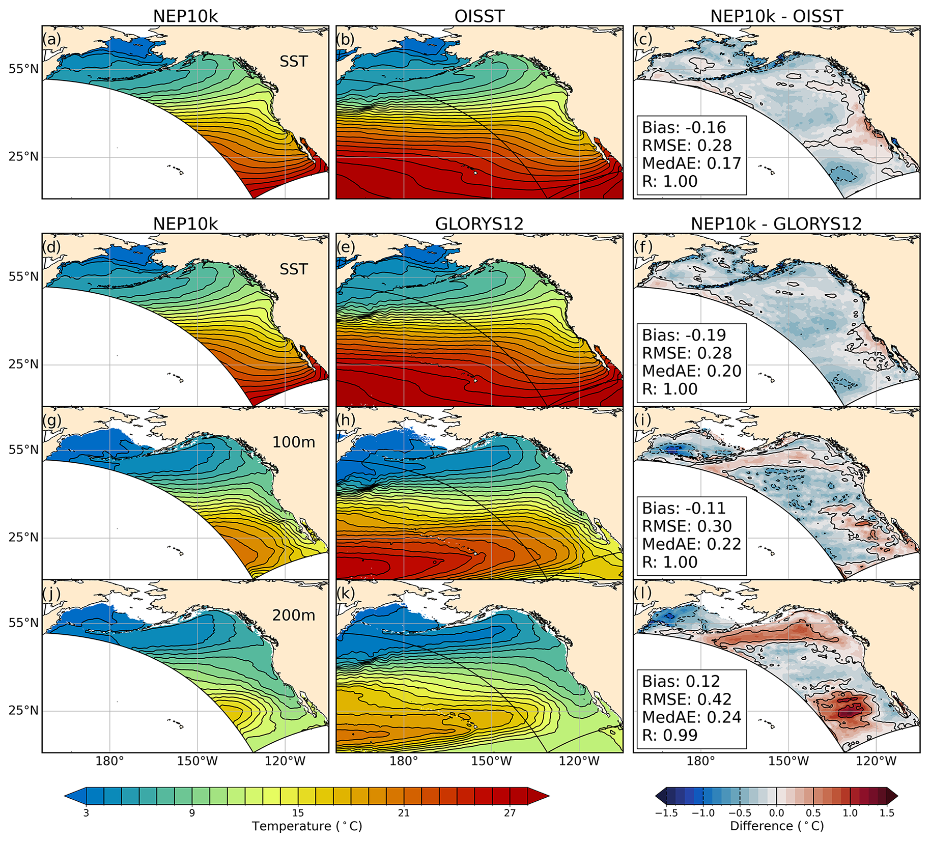
Figure 2Temperature comparisons. Annual mean surface and subsurface (100 m, 200 m) temperature compared against NOAA OISSTv2.1 and the GLORYS12 reanalysis. Values in the left two columns represent the average of the annual means covering 1993 through 2019. The right column depicts the difference between NEP10k and the respective validation product, along with the area-weighted mean bias, root mean squared error (RMSE), medium absolute error (MedAE), and Pearson correlation coefficient (R). The NEP10k model domain below 66° N is outlined in black. Panels a and d show the same model output.
Similar to temperature, NEP10k broadly reproduces annual mean salinity fields found in regional climatologies and GLORYS12, with the majority of the domain falling within 0.25 practical salinity units (PSU) of the reference datasets (Fig. 3). Notable fresh surface biases exceeding 0.5 PSU occur along the coast in the Gulf of Alaska, eastern Bering Sea, and northern CCS, coincident with regions of substantial freshwater inputs from rivers and glacial melt (Fig. 3c and l). Positive salinity biases relative to GLORYS12 occur in the western Bering Sea at the surface and 100 m and over all depths in the southwest region of the domain (Fig. 3, right panels). In the latter case, the salty bias coincides with warm biases (Fig. 2). Seasonally, similar generally modest biases can be seen in the Boreal winter (Fig. S3) and summer (Fig. S4 in the Supplement) equivalents.
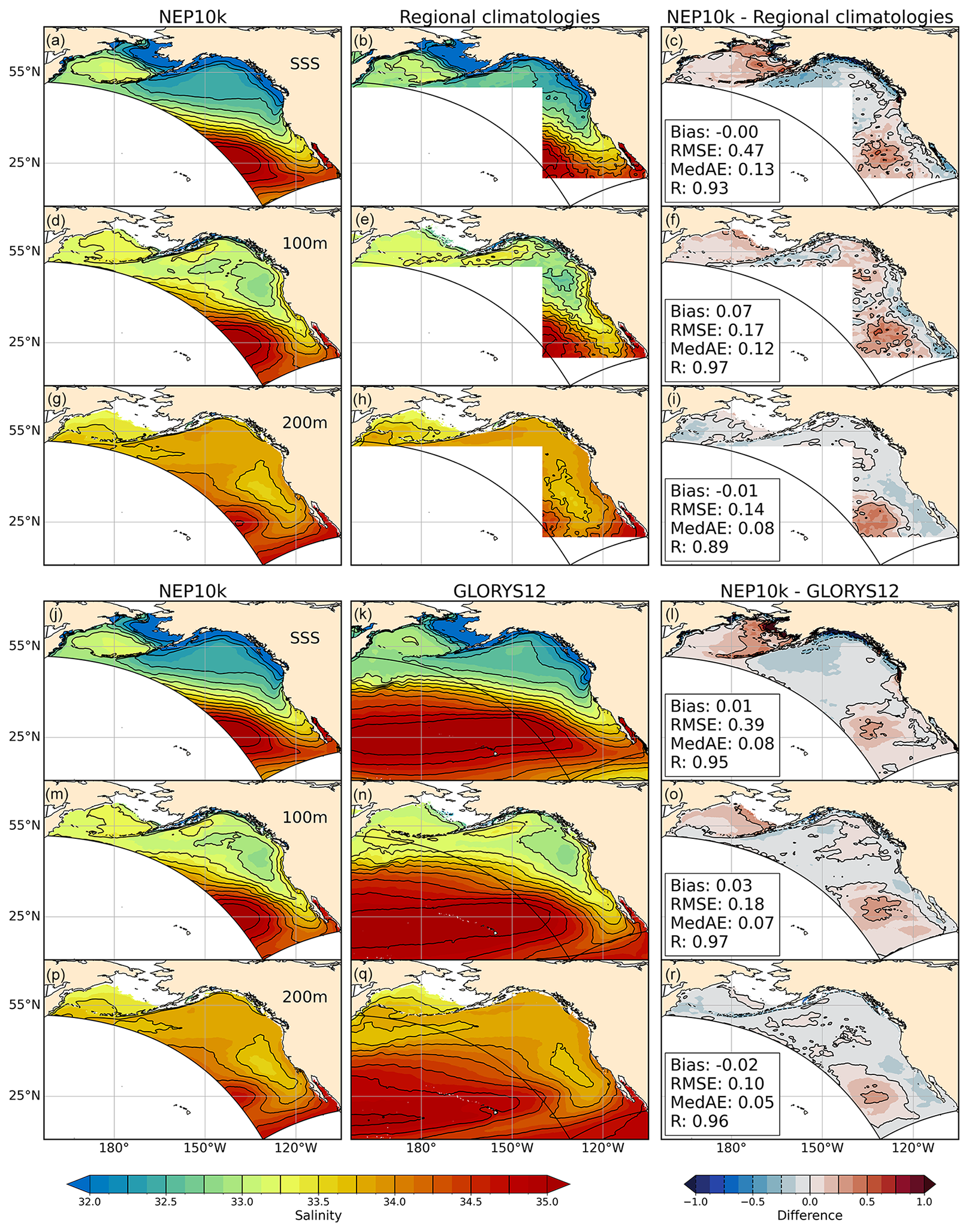
Figure 3Salinity comparisons. Annual mean surface and subsurface (100 m, 200 m) salinity compared against NCEI regional ocean climatologies and the GLORYS12 reanalysis. The regional climatologies are a composite of the northeast Pacific (nep) and northern North Pacific (nnp) climatologies. The nep climatology extends from 1995 to 2012, while the updated nnp climatology (Version 2) covers 1995–2014. Where the two regional climatologies overlap in the GOA (i.e., above 50° N), we use the more recent nnp climatology. For comparison against the model, we use the same years of NEP10k, with panels (a), (d), and (g) showing the model values for average annual mean salinities for 1995–2014 above 50° N (as opposed to average annual mean salinities for 1995–2012 below 50° N). The comparison against GLORYS12 (bottom three rows) covers 1993–2019. Area-weighted bias, root mean squared error (RMSE), median absolute error (MedAE), and Pearson correlation coefficient (R) are reported in the right column of figures, depicting the difference between NEP10k and the respective validation product.
Mixed layer depth in NEP10k, defined as the depth at which density is 0.03 kg m−3 greater than at 5 m depth, exhibits a modest shallow/negative bias relative to the estimates of de Boyer Montégut (2024), with deeper (positive) biases occurring in the interior ocean near the Bering shelf break (Fig. 4, top row). These biases are amplified and reduced during Boreal winter (JFM, Fig. S5 in the Supplement, top row) and summer (JAS, Fig. S6, top row), respectively, when mixing drivers (i.e., surface heating/cooling, wind, and storm intensity) are correspondingly modified. Conversely, NEP10k exhibits a positive mean bias when compared against GLORYS12 MLD, which is particularly pronounced in the Bering Sea (Fig. 4, bottom row) and exhibits a reverse seasonal response (i.e., reduced positive bias in the winter and increased in the summer; Figs. S5 and S6 in the Supplement, bottom row). With the exception of the deep/positive winter biases in the Bering Sea, the model represents MLD spatial variability fairly well, with significant (p<0.001) correlations exceeding 0.85 across all seasons and comparisons (Figs. 4, S5, and S6).
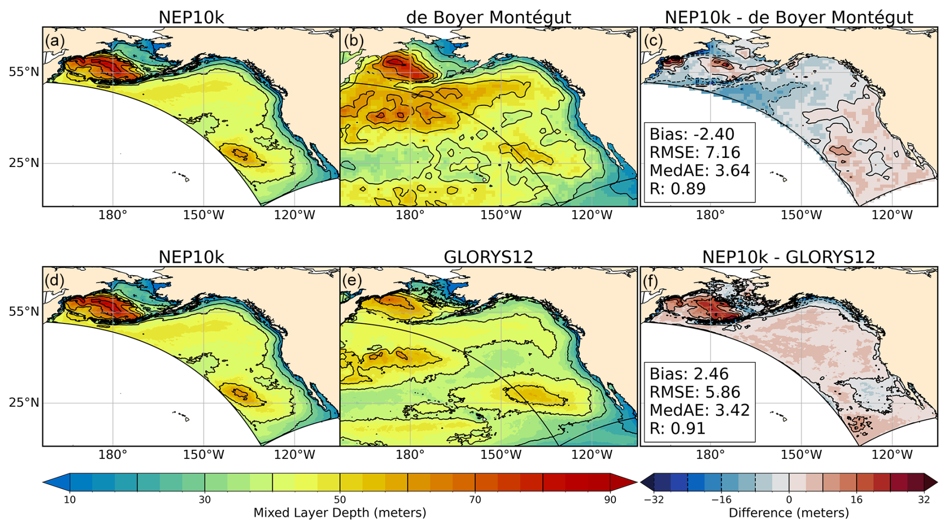
Figure 4Mixed layer depth comparisons. Climatological mean of mixed layer depth compared against de Boyer Montégut (a–c) and GLORYS (d–f). Black reference contours in (a), (b), (d), and (f) are depicted at 5 m intervals and at 8 m intervals in (c) and (f); contours depicting negative values in (c) and (f) are drawn with dashed lines. Area-weighted bias, root mean squared error (RMSE), median absolute error (MedAE), and Pearson correlation coefficient (R) are reported in the right column of figures, depicting NEP10k-respective reference products. All values represent the annual mean for years 1993 through 2019, and the extent of the NEP10k domain is outlined in black in all figures. Panels a and d show the same model output.
SSH gradients in the NEP10k hindcast are broadly consistent with GLORYS12 and CMEMS satellite altimetry (Fig. 5), exhibiting the lowest values along the Aleutian island chain, in the GOA, and in the western Bering Sea and the highest values near 25° N along the western edge of the domain. Similar to satellite measurement and GLORYS12, NEP10k also exhibits relatively low SSH along the U.S. West Coast (compared with offshore SSH values at the same latitude), a signature of coastal upwelling. However, the SSH gradients in NEP10k are smaller along the Aleutian island chain than exhibited in the reference datasets. There is a notable correspondence of this SSH gradient bias with the Gulf of Alaska subsurface temperature biases noted in Fig. 2, suggesting a potential relationship between these two features.
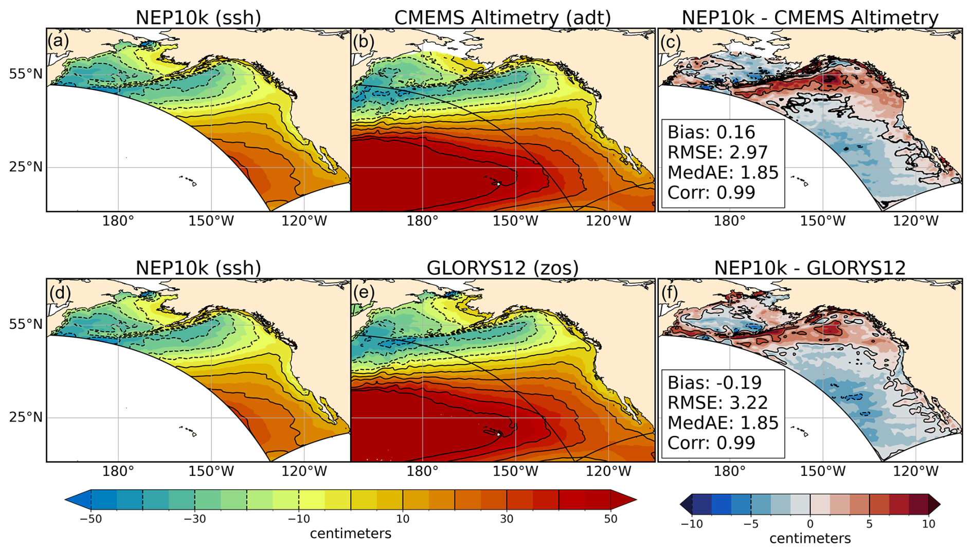
Figure 5Sea surface height comparisons. NEP10k average-centered, climatological mean sea surface height comparison for NEP10k (a, d; identical panels), GLORYS12 (b), CMEMS satellite altimetry (e), and their respective differences (c, f). All values represent the annual mean (1993–2019). Area-weighted mean bias (Bias), root mean squared error (RMSE), median absolute error (MedAE), and Pearson correlation coefficient (R) are reported in the right column of figures, depicting the difference between NEP10k and the comparison product; all correlations are significant (p<0.001). The reference height contours in all panels are drawn at 0.1 and 0.05 m intervals for the mean and difference plots, respectively, with negative values shown as dashed lines. All panels show the extent of the NEP10k domain as a black outline.
Compared against the TPXO dataset, which was used as the tidal boundary forcing conditions, NEP10k reproduces tidal amplitude and phases in the domain interior with high fidelity (Fig. 6). The greatest tidal amplitude discrepancies occur in the nearshore regions of the eastern Bering Sea (Fig. 6c and f) and partially enclosed features (e.g., northern Gulf of California and Cook inlet; Fig. 6c). Amplitude biases for the most prominent semidiurnal (M2) and diurnal (K1) constituents in these nearshore and partially enclosed regions can exceed 20 cm and 10 cm, respectively. These regions, however, also have the largest overall amplitudes, with values exceeding 1 m and 50 cm, respectively. Such nearshore tidal biases are not surprising given the relatively coarse 10 km resolution enlisted herein, and we note that skillful tidal simulations extend all the way to the coast in most regions. To investigate some of these biases further, we include additional zoomed-in maps of the eastern Bering Sea and western Gulf of Alaska in the Supplement (Fig. S12), along with comparison against several tide gauges in that region. Both TPXO and NEP10k perform well at most tide gauges. Generally, TPXO better approximates tidal harmonic constituents than NEP10k, with higher Pearson correlation coefficients and/or lower RMSE (with the exception of the M2 phase). However, in cases such as the gauge in Anchorage, AK, the bias in M2 amplitude for TPXO is comparable to the bias exhibited by NEP10k. Because these biases have opposite signs, the discrepancy between the two gridded products (i.e., NEP10k-TPXO, shown in the maps in Figs. 6 and S12) exaggerates the model bias by almost a factor of 2 relative to the bias for the gauge. Thus, some of the more severe nearshore differences in Fig. 6 may be a reflection of how NEP10k and TPXO approximate complex coastline geometry (bottom of Fig. S13 in the Supplement) rather than an exact indication of NEP10k performance.
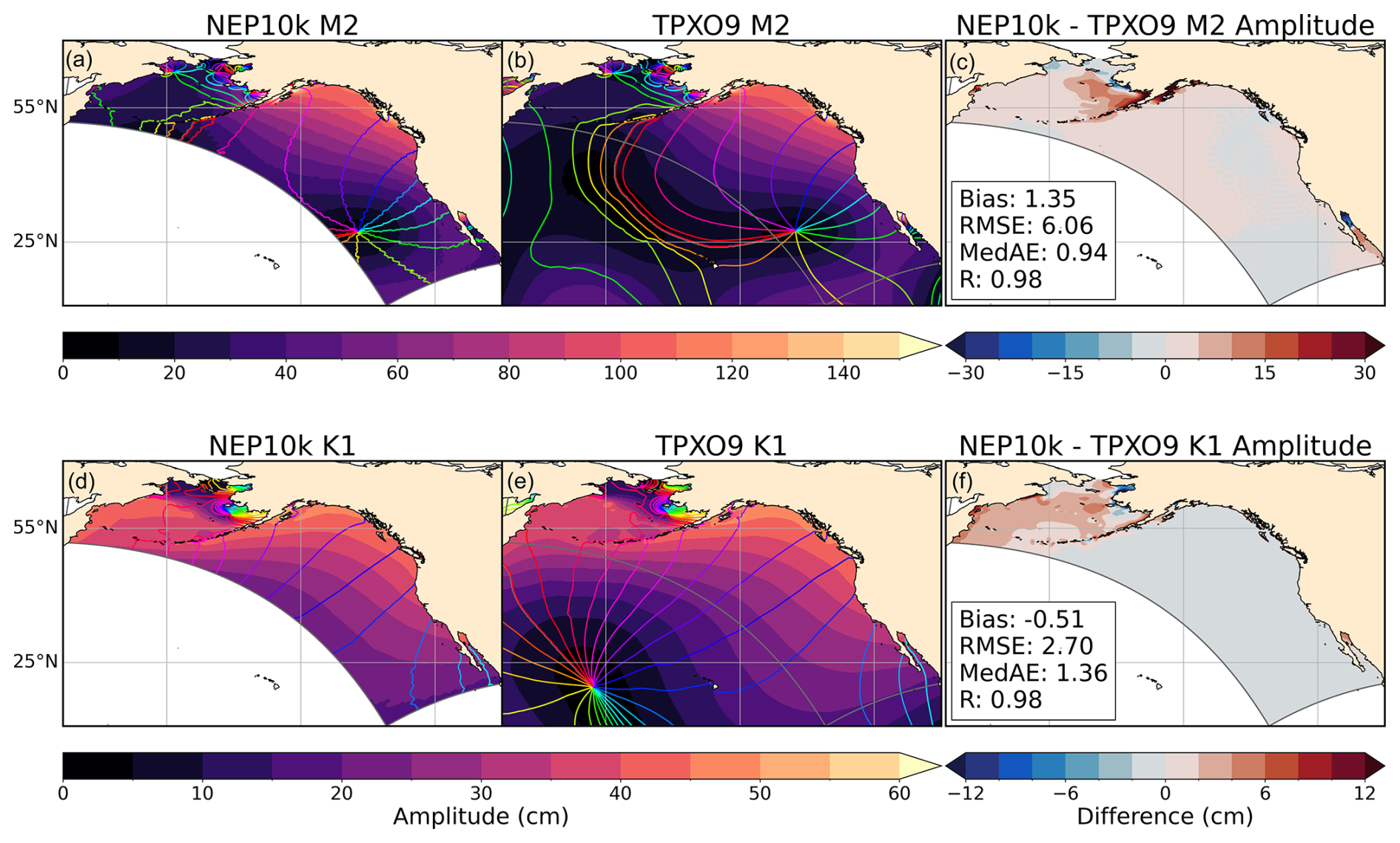
Figure 6M2 and K1 tidal amplitudes and period. Comparison of tidal constituents M2 (top row) and K1 (bottom row) in NEP10k against those in the TPXO9 forcing dataset. Filled contours depict the tidal amplitude, while overlain colored contours depict the tidal phase for the given constituent. Filled contours in the difference plot (c, f) show the difference in amplitude only; bias, root mean squared error (RMSE), median absolute error (MedAE), and Pearson correlation coefficient (R) are also reported in these panels. The extent of the NEP10k domain is outlined in gray in all figures.
3.1.2 Large-scale biogeochemical and ecosystem properties
Macronutrient concentrations (nitrate and phosphate) exhibit large-scale agreement with annual World Ocean Atlas nutrients, but significant regional biases are also apparent (Figs. 7 and 8). The largest high bias occurs along the Aleutian island chain and Bering Sea shelf break. In the simulation, the region of elevated surface nutrients observed in the central Bering Sea extends further south and east in the model. These biases correspond with the most prominent region of overmixing (Fig. 4). Positive surface nitrate and phosphate biases in affected regions exceed 5 µmol kg−1 NO3 and 0.25 µmol kg−1 PO4, respectively, and extend with lesser severity onto the Bering shelf. The positive surface bias is underlain by negative nitrate and phosphate biases at 200 m, reinforcing the likelihood that the surface high macronutrient bias is linked to excessive mixing rather than excessive nutrients in underlying source waters. Uncertainty in nitrogen removal processes in shallow Bering shelf sediments (e.g., denitrification and burial) may also play a role in the perpetuation of biases onto the shelf. Macronutrient concentrations in Gulf of Alaska surface waters, in contrast, are biased low by 1.5–3 µmol kg−1 NO3 and 0–0.375 µmol kg−1 PO4, respectively (Figs. 7c and 8c), despite exhibiting a combination of positive and negative biases at depth. These biases are consistent with shallow mixed layer biases in the Gulf of Alaska (Fig. 4). Finally, the California Current exhibits a modest positive surface macronutrient bias. Despite these discrepancies, the simulation generally exhibits high correlations with observed macronutrients (R>0.96) and RMSEs that are only ∼5 % of the dynamic range of the macronutrient concentrations across the west coast ecosystems. This skill extends to seasonal patterns with correlation values exceeding 0.8 and RMSE<10 % of the dynamic range in all cases (Figs. S9–S12 in the Supplement). Notably, winter and summer nitrate conditions exhibit more pronounced bias patterns relative to the mean state, with particularly high levels in the Bering surface waters and low levels in portions of the Gulf of Alaska (Figs. S9c and S10c). Conversely, surface phosphate levels over the Bering shelf are biased low in the winter and high in the summer (Figs. S11c and S12c). Summer surface nitrate levels along the California Current Ecosystem (CCE) (Fig. S10c) are potentially suggestive of overrepresentation of summer upwelling.
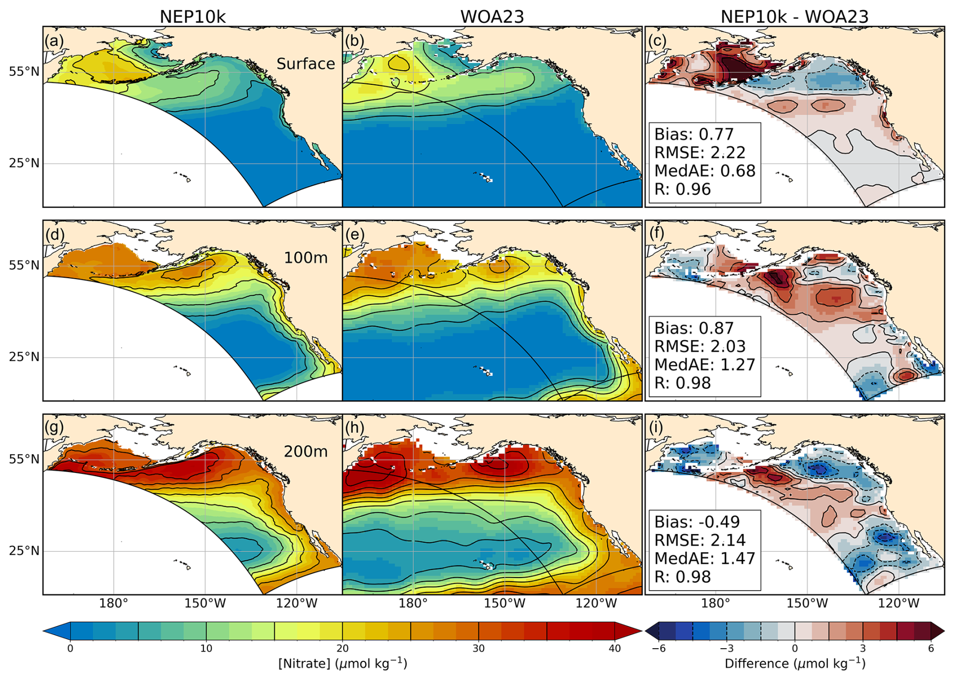
Figure 7Nitrate comparisons. Annual mean surface and subsurface (100 m, 200 m) nitrate compared against WOA23. Comparison time frames cover 1993–2019. Reference contours are depicted in black at 5 and 1.5 µmol nitrate per kg sea water in the mean state (left and center columns a, b, d, e, g, h) and difference (right column c, f, i) plots; contours representing negative values in the difference plot are drawn as dashed lines. Bias, root mean squared error (RMSE), median absolute error (MedAE), and Pearson correlation coefficient (R) are reported in the right column (c, f, i) of figures, depicting the difference between NEP10k and WOA23. The extent of the NEP10k domain is outlined in black in all figures.
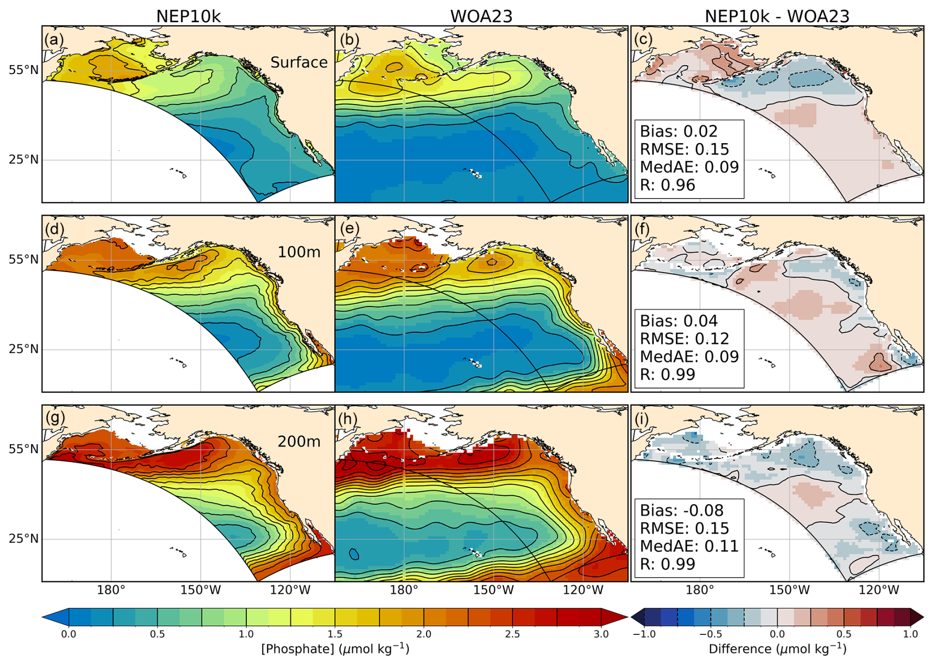
Figure 8Phosphate comparisons. Annual mean surface and subsurface (100 m, 200 m) phosphate compared against WOA23. Comparison time frames cover 1993–2019. Reference contours are depicted in black at 0.25 µmol phosphate per kg sea water in the mean state (left and center columns a, b, d, e, g, h) and difference (right column c, f, i) plots; contours representing negative values in the difference plot are drawn as dashed lines. Bias, root mean squared error (RMSE), median absolute error (MedAE), and Pearson correlation coefficient (R) are reported in the right column (c, f, i) of figures, depicting the difference between NEP10k and WOA23. The extent of the NEP10k domain is outlined in black in all figures.
While macronutrients play an important role in the biogeochemistry and ecosystem dynamics of the NEP, iron has been observed to be a limiting or co-limiting nutrient (Browning et al., 2017; Browning and Moore, 2023). The simulated distribution of surface iron exhibits a gradient from inshore highs exceeding 1 nmol kg−1 to offshore lows <0.25 nmol kg−1 (Fig. 9, left panel). This distribution of dissolved iron results in large-scale patterns of phytoplankton iron limitation in the NEP10k simulation (Fig. 9, right panel) that are consistent with those observed (e.g., Moore et al., 2013; Hutchins et al., 1998).
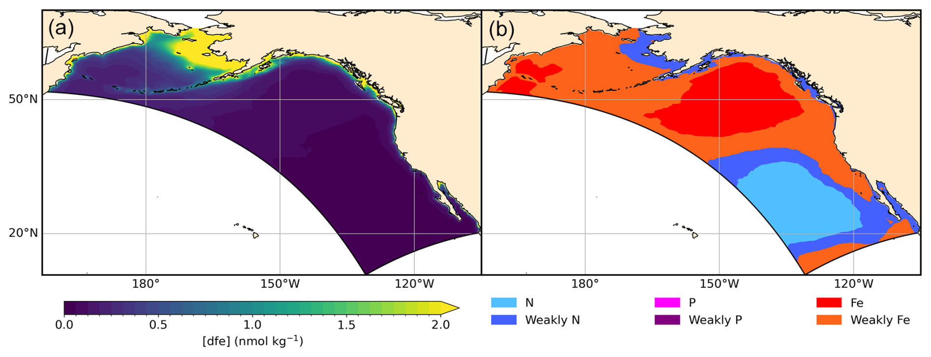
Figure 9Surface dissolved iron and phytoplankton nutrient limitation. NEP10k simulated annual mean surface dissolved iron concentrations (a) and climatological mean distribution of the nutrient most limiting to phytoplankton growth (b). In COBALT, the degree of limitation by N, P, and Fe is expressed as a factor between 0 and 1 (Stock et al., 2020). Nutrient limitation is then calculated according to Liebig's law of the minimum. This most limiting nutrient is indicated in the figure below. We further differentiate areas where the N, P, or Fe limitation term is less than 0.25 more limiting than another nutrient, which effectively indicates areas that are near co-limitation. Time frame covers 1993–2019. Note: Sparse P limitation occurs nearshore.
Simulated surface chlorophyll is spatially well correlated with satellite-based chlorophyll estimated from the OC-CCI (Fig. 10), and simulated values are generally within a factor of 2 of those observed, which span 2 orders of magnitude (i.e., the RMSE of the log10-transformed data is less than 0.3 in all seasons). The simulation, however, is generally biased high in the Gulf of Alaska and Bering Sea in the boreal spring and summer, with biases exceeding a factor of 2 along the Bering Sea shelf break and along the subpolar/subtropical boundary in the Gulf of Alaska. The model underestimates the OC-CCI-based chlorophyll concentration during the fall and winter on the eastern Bering Sea shelf: while NEP10k-COBALTv3 suggests lower chlorophyll concentrations during these cold and dark periods, OC-CCI estimates remain high in nearshore waters. Indeed, satellite-based estimates suggest higher chlorophyll along the Bering coast in fall and winter than in spring and summer. It is notable, however, that satellite-based chlorophyll estimates are sporadic at high latitudes during these seasons, and OC-CCI uses a chlorophyll estimation algorithm developed primarily for “case 1”/oceanic water. Vigorously mixed, turbid waters along the Bering shelf in winter undoubtedly depart considerably from the algorithm's high degree of water transparency assumptions. In the CCE, the model is able to match the juxtaposition of coastal chlorophyll highs and subtropical offshore lows estimated by OC-CCI during the spring and summer upwelling period. Elevated chlorophyll levels do extend further offshore in the simulation than satellite estimates suggest. Values are also elevated near the domain boundary during this period, likely due to some spurious boundary mixing. Fall and winter conditions in the California Current exhibit a moderate positive bias in offshore waters that generally falls below a factor of 2.
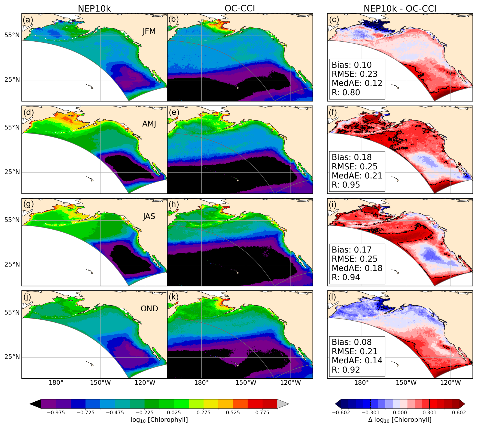
Figure 10Surface chlorophyll comparisons. Seasonal means of surface chlorophyll compared with OC-CCI satellite observations. The 3-month seasonal periods include January through March (JFM, a–c), April through June (AMJ, d–f), July through September (JAS, g–i), and October through December (OND, j–l). Comparison time frames cover 1998–2019; all chlorophyll values were log10-transformed prior to temporal averaging. Bias, root mean squared error (RMSE), median absolute error (MedAE), and Pearson correlation coefficient (R) are reported in the right column (c, f, i, l) of figures, depicting the difference between NEP10k and OC-CCI. Black contours in the right column (c, f, i, l) indicate where the difference . The extent of the NEP10k domain is outlined in gray in all figures.
Moving up the food web, simulated seasonal mesozooplankton biomass concentrations (Fig. 11) exhibit similar large-scale spatial and seasonal patterns as the COPEPOD database (Moriarty and O'Brien, 2013). The patchiness of the observations reduces correlations relative to the smoother physical, nutrient, and satellite-based chlorophyll estimates compared thus far (R≥0.30 for all seasons). However, peak summer concentrations (∼50 mg C m−3) consistent with observed values are evident in the Bering Sea and inshore regions of the Gulf of Alaska in both the model and observations. These highs contrast sharply with observed and modeled values (∼1–2 mg C m−3) within the North Pacific subtropical gyre. Intermediate values of ∼10–20 are evident in the California Current upwelling. Both the observed and modeled values are highest during the peak summer upwelling period, though the highest modeled values are somewhat lower, particularly in nearshore regions. This pattern will be addressed further in the Discussion section. The offshore waters of the Gulf of Alaska and western Bering Sea exhibit summer mesozooplankton biomass peaks of similar magnitude as the California Current, with simulated values again lower yet comparable to those observed.
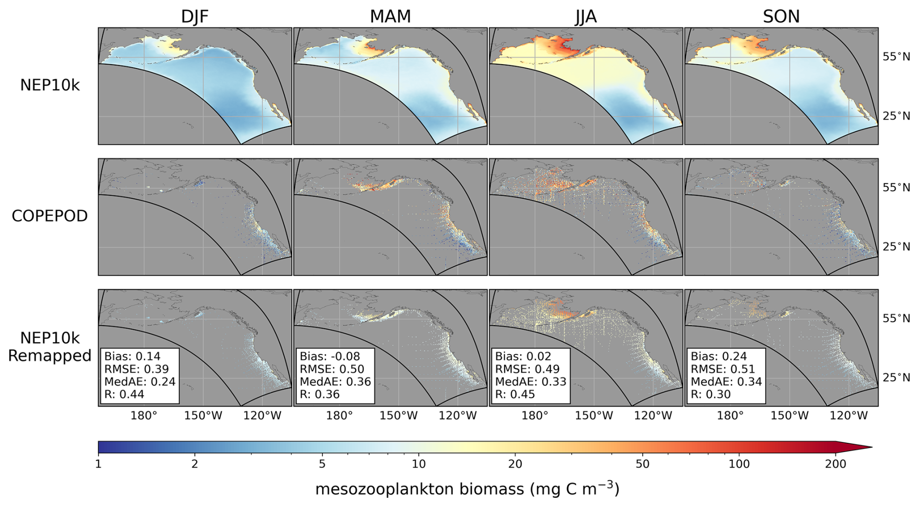
Figure 11Seasonal zooplankton biomass. Seasonal mean mesozooplankton biomass concentrations for NEP10k on the model grid (top row), the COPEPOD dataset (middle row), and NEP10k values remapped to the COPEPOD grid where there are corresponding data from the COPEPOD dataset (bottom row). The bottom row also reports statistics using the log10 normalized data, specifically the area-weighted mean bias (Bias, NEP10k – COPEPOD), the area-weighted root mean squared error (RMSE), the median absolute error (MedAE), and the Pearson correlation coefficient (R); all correlation values are significant (p<0.001). Maps are plotted with a gray background to increase contrast with the patchy observation data.
Simulated oxygen concentrations in the top 200 m in the NEP10k are generally spatially consistent with WOA (Fig. 12). Some biases, however, are apparent below the surface. Most notably, the model has a low oxygen bias south of the Aleutian Islands at 100 m (Fig. 12f). This bias coincides with a warm water bias (Fig. 2) and is overlain by a fresh/high stratification bias (Figs. 3 and 4). As noted above, this is the region where the westward flowing Alaska Stream and eastward flowing North Pacific Current interact, suggesting that the biases may be linked to a suboptimal representation of these two currents. Moderately high oxygen biases (i.e., greater than 25 µmol kg−1) are apparent in the western Bering Sea, eastern Gulf of Alaska, and off of Baja at 200 m (Fig. 12i), but none are large enough to compromise NEP10k's large-scale fidelity to the observed oxygen distribution in the top 200 m (i.e., R values≥0.9 across depths and seasons; Figs. 12, S14, and S15 in the Supplement).
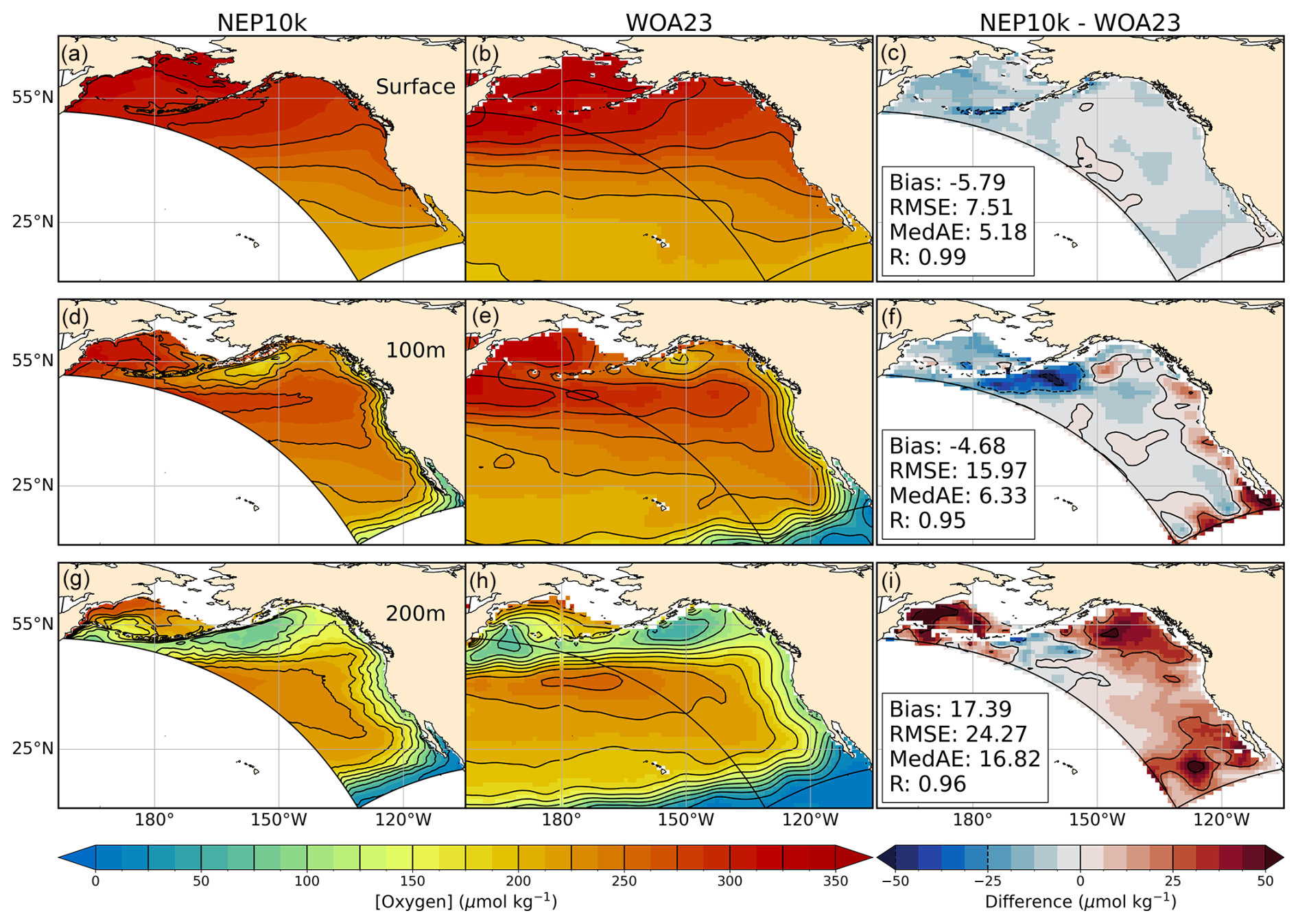
Figure 12Dissolved oxygen comparisons. Annual mean surface and subsurface (100 m, 200 m) dissolved oxygen compared against WOA23. Comparison time frames cover 1993–2019. Reference contours are depicted in black at 25 µmol oxygen per kg sea water in the mean state (left and center columns a, b, d, e, g, h) and difference (right column c, f, i) plots; contours representing negative values in the difference plot are drawn as dashed lines. Bias, root mean squared error (RMSE), median absolute error (MedAE), and Pearson correlation coefficient (R) are reported in the right column (c, f, i) of figures, depicting the difference between NEP10k and WOA23. The extent of the NEP10k domain is outlined in black in all figures.
Deeper in the water column, NEP10k robustly simulates the cross-ecosystem variation in the depth of the hypoxic boundary (i.e., the depth at which the oxygen concentration drops below 61.7 µmol oxygen per kg sea water; see Fig. 13). The hypoxic boundary is shallowest, approaching 100 m from the surface, along the southern domain boundary, which lies along the periphery of the broader eastern equatorial Pacific hypoxic zone. The hypoxic boundary then descends progressively to ∼400 m in both the model and observations as one moves northward along the California Coast into Canada, before shoaling again to ∼150 m in the northern Gulf of Alaska. While these overall patterns are consistent, the biases discussed in Fig. 12 are echoed in the hypoxic boundary layer depth. The boundary layer is deeper in the western Bering Sea, eastern Gulf of Alaska, and Southern CCS but biased shallow south of the Aleutian island Chain and, to a lesser degree, in the northern-to-central CCS.
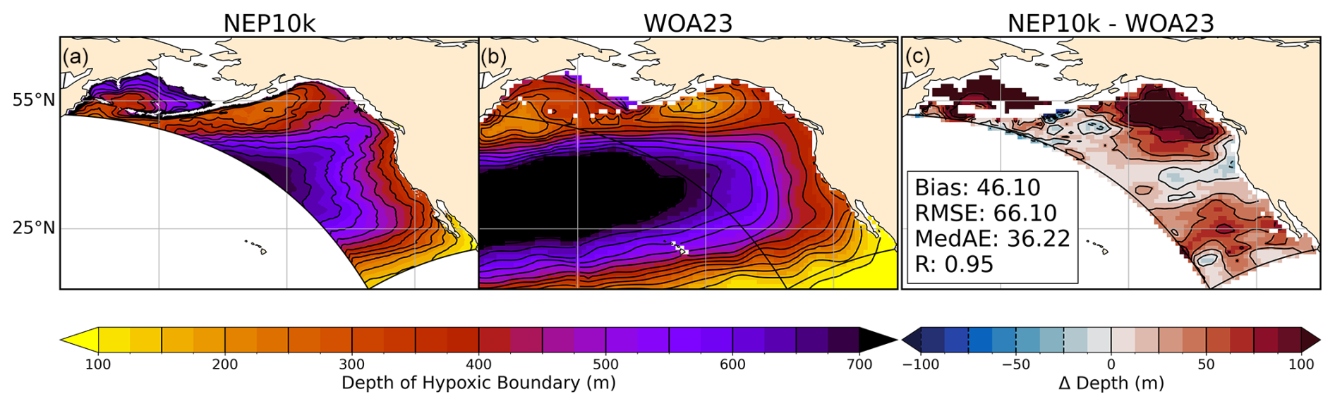
Figure 13Hypoxic boundary layer depth. Annual mean hypoxic boundary layer depth (i.e., depth at which the dissolved oxygen concentration drops below 61.7 µmol oxygen per kg sea water) compared against WOA23. Black reference contours indicate 150 m and 25 m intervals in the mean state (a, b) and difference (c) plots; contours representing negative values in (c) are drawn as dashed lines. Area-weighted mean bias (Bias), root mean squared error (RMSE), median absolute error (MedAE), and Pearson correlation coefficient (R) are reported in panel (c). The extent of the NEP10k domain is outlined in black in all figures.
Finally, simulated carbon chemistry patterns (total alkalinity, dissolved inorganic carbon (DIC), and aragonite saturation state; Figs. 14–16) broadly capture observation-based estimates reported in CODAP-NA. Low coastal surface alkalinity patterns consistent with low alkalinity river inputs are apparent in the Gulf of Alaska and, to a lesser degree, the eastern Bering Sea. Simulated alkalinity increases from these lows toward maximal values in the North Pacific gyre in a manner consistent with observations, though the simulated values are biased high (Fig. 14a–c). The largest positive surface alkalinity biases occur in the western Bering Sea and in the southwest corner of the domain. These surface alkalinity biases are aligned with positive salinity biases that penetrate to depth (Fig. 3). The largest subsurface bias, however, occurs at a depth of 100 m in the Gulf of Alaska near the large freshwater outflows in the Gulf of Alaska. This bias distribution suggests that the low alkalinity freshwater signal in this region may be overly restricted to the surface in the model, though there does not appear to be a strong positive subsurface salinity model bias in this region (Fig. 3).
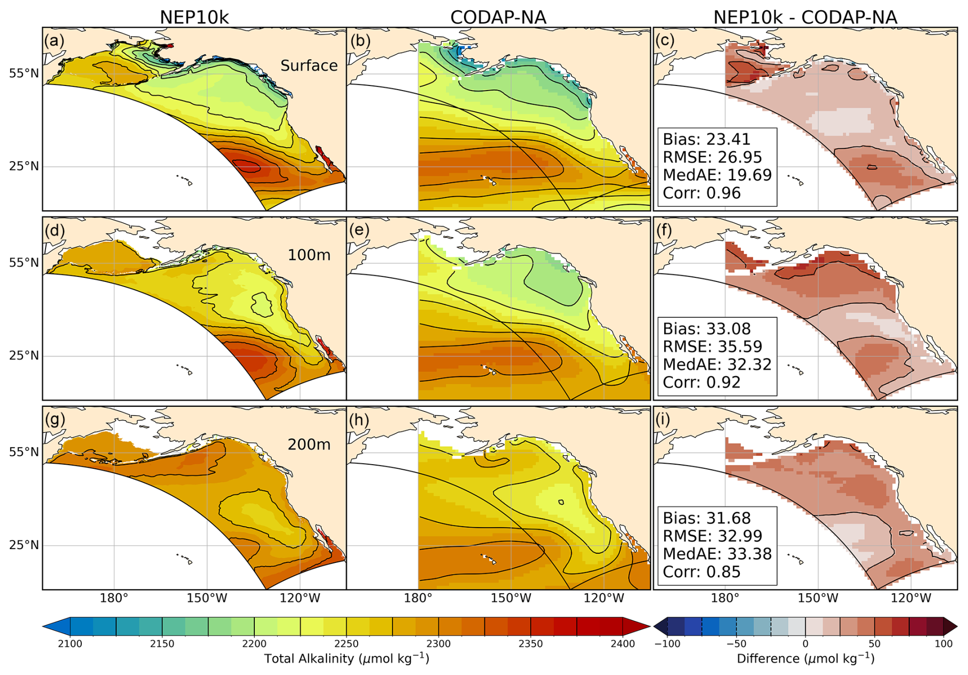
Figure 14Total alkalinity comparisons. Annual mean surface and subsurface (100 m, 200 m) total alkalinity compared against CODAP-NA. Comparison time frames cover 2004–2018. Reference contours are depicted in black at 25 µmol alkalinity per kg sea water in the mean state (left and center columns a, b, d, e, g, h) and difference (right column c, f, i) plots. Area-weighted mean bias (Bias), root mean squared error (RMSE), median absolute error (MedAE), and Pearson correlation coefficient (R) are reported in the right column (c, f, i) of the difference plots. All correlation values are significant at p<0.001. The extent of the NEP10k domain is outlined in black in all figures.
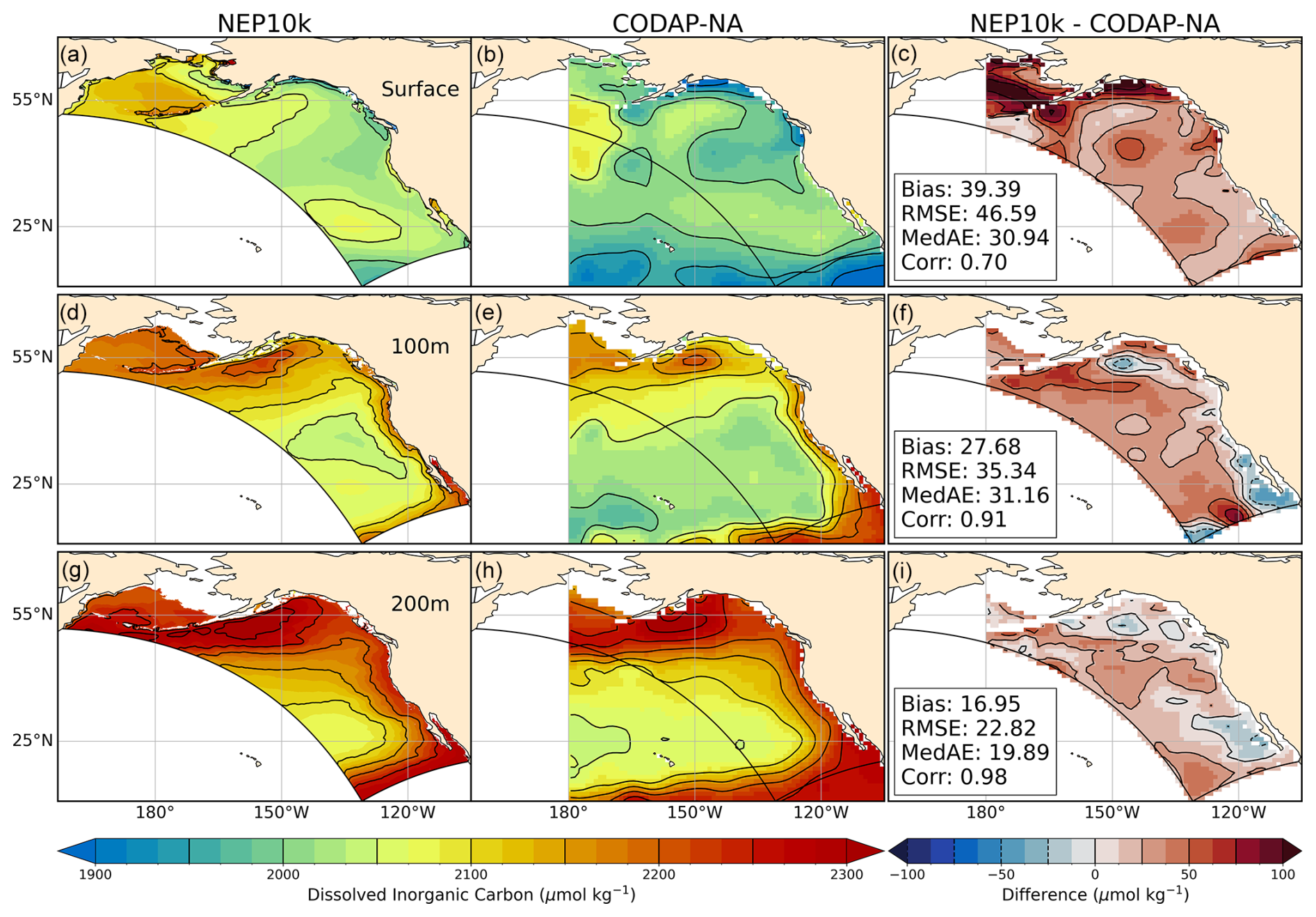
Figure 15Dissolved inorganic carbon comparisons. Annual mean surface and subsurface (100 m, 200 m) concentration of dissolved inorganic carbon compared against CODAP-NA. Comparison time frames cover 2004–2018. Reference contours are depicted in black at 50 and 25 µmol carbon per kg sea water in the mean state (left and center columns a, b, d, e, g, h) and difference (right column c, f, i) plots; contours representing negative values in the difference plots are drawn as dashed lines. Area-weighted mean bias (Bias), root mean squared error (RMSE), median absolute error (MedAE), and Pearson correlation coefficient (R) are reported in the right column (c, f, i) of the difference plots. All correlation values are significant at p<0.001. The extent of the NEP10k domain is outlined in black in all figures.
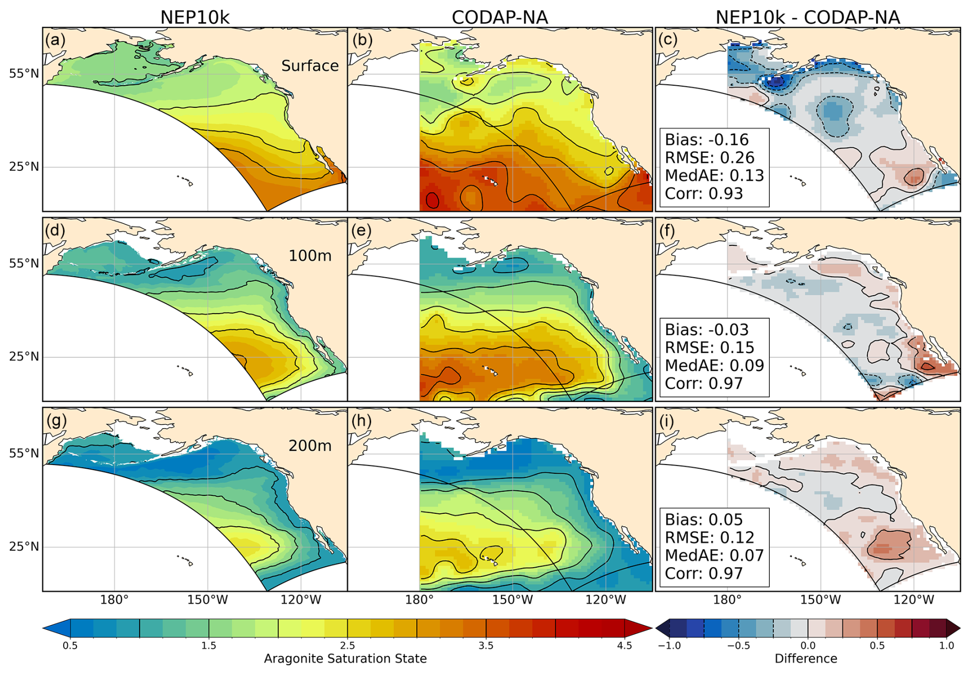
Figure 16Aragonite saturation state comparisons. Annual mean surface and subsurface (100 m, 200 m) aragonite saturation state compared against CODAP-NA. Comparison time frames cover 2004–2018. Reference contours are depicted in black at 0.5 and 0.25 saturation state units in the mean state (left and center columns a, b, d, e, g, h) and difference (right column c, f, i) plots; contours representing negative values in the difference plots are drawn as dashed lines. Area-weighted mean bias (Bias), root mean squared error (RMSE), median absolute error (MedAE), and Pearson correlation coefficient (R) are reported in the right column (c, f, i) of the difference plots. All correlation values are significant at p<0.001. The extent of the NEP10k domain is outlined in black in all figures.
Dissolved inorganic carbon has a high bias that is consistent with the high alkalinity bias (compare Figs. 14 and 15). Like alkalinity, the largest positive biases occurred along the Bering Sea shelf break and in the southwestern corner of the domain where areas are overmixed (Fig. 4) and exhibit salty biases (Fig. 3). The high surface DIC bias in the northern Gulf of Alaska, however, is more pronounced than the corresponding high surface alkalinity bias in this region (i.e., Fig. 13c vs. Fig. 14c). The northern Gulf of Alaska is strongly impacted by river and glacial outflows. While some of these freshwater sources (e.g., the Copper and Susitna rivers) have observational constraints on DIC and Alk, most do not. Improved constraints may be needed to improve the model fit in this region.
The more-pronounced high surface DIC bias in the northern Gulf of Alaska yields aragonite saturation states that are 0.25–0.5 units lower than the CODAP-NA product (Fig. 16). The overall gradient between low saturation states (higher acidification vulnerability) in the surface waters of the Bering Sea/Gulf of Alaska to high saturation states (lower acidification vulnerability) in equatorial and subtropical surface waters in the southern parts of the domain, however, is well captured (Fig. 15c, R=0.93). Saturation state biases are also small in subsurface waters where subsaturated waters are more prevalent (Fig. 16, middle and bottom panel) and where valuable shell, crab, and demersal fisheries reside.
3.2 Region-specific evaluation
The evaluation of NEP10k against observed large-scale physical and biogeochemical patterns in Sect. 3.1 was generally favorable. In all cases, the model was able to capture the primary physical, biogeochemical, and plankton contrasts across ecosystems within the broad NEP10k domain with often high but at least moderate fidelity. As described in Sect. 1, however, the NEP10k configuration is intended for marine resource applications both across and within NEP10k subregions and across management-relevant time horizons from seasons to multiple decades. The evaluation in Sect. 3.1 provides a foundation for such applications but is not sufficient. The evaluation in this section focuses on regional fisheries-critical metrics and their variation across management-relevant seasonal to multidecadal time horizons.
Perhaps the most ubiquitous indicators of ecosystem state across all regions are ocean temperature (surface and bottom) and surface chlorophyll. These indicators are highly relevant to diverse aspects of ecosystem function, and long time series of observation-informed estimates are available. Modeled shelf (where depth <500 m) surface and bottom temperature climatologies for the regions identified in Fig. 1 exhibit high correlation (Fig. 17, left column) with GLORYS12, but surface temperatures tend to be biased warm in more southerly regions. As initially illustrated in Figs. 2 and S2, mean and summer surface temperatures, respectively, in the central and southern California Current System are 1–2 °C warmer than those observed, but biases in other regions tend to be <1 °C.
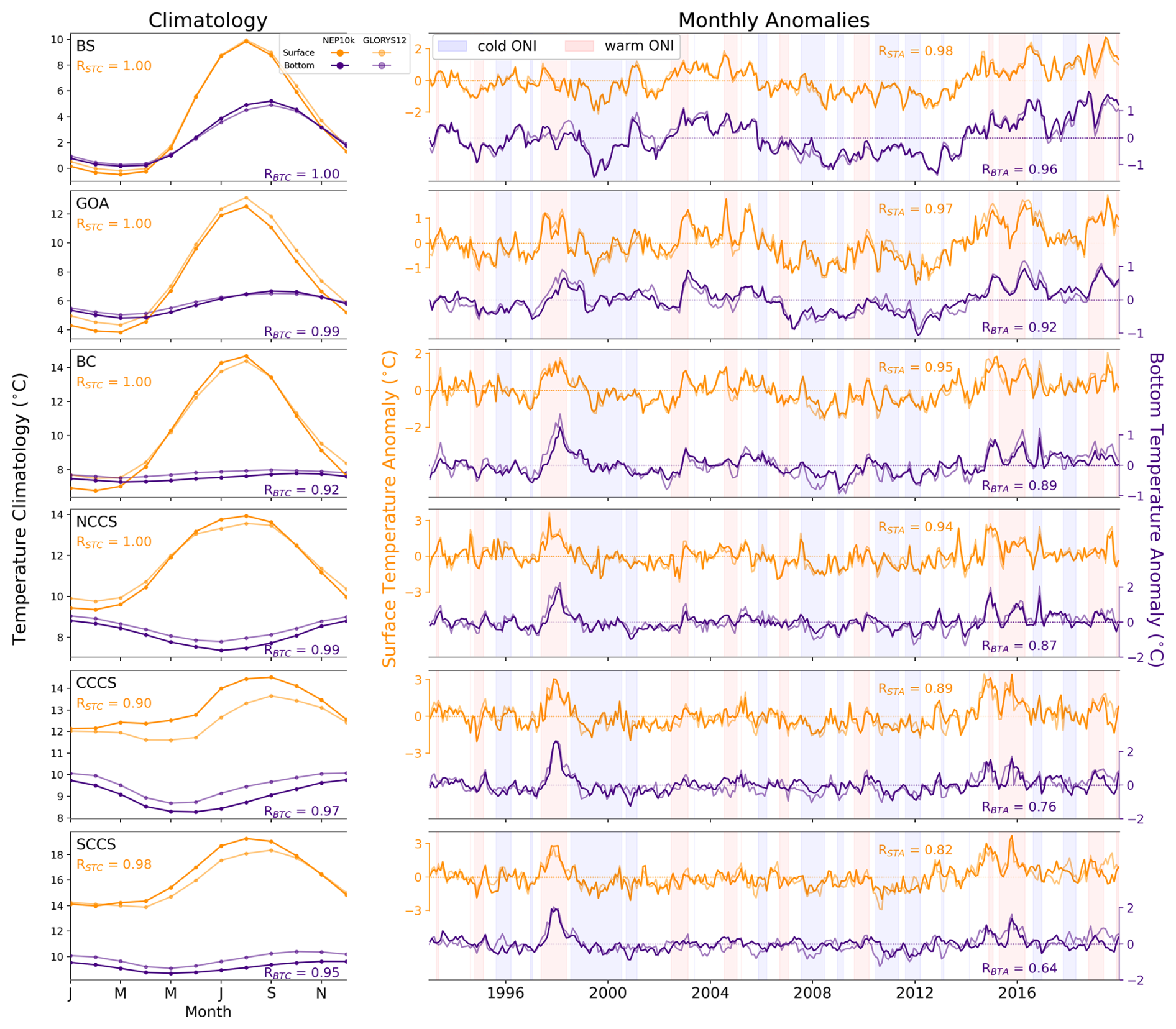
Figure 17Surface and bottom temperature comparisons for shelf (0–500 m) regions. Regional shelf (depth ≤500 m) surface and bottom temperature climatologies (left column) and anomaly time series (right column) for the subregions delineated in Fig. 1. Comparison of temperature climatologies (left panels) and monthly anomalies (right panels) for surface (orange) and bottom (purple) temperatures for NEP10k (bold) and GLORYS12 (pale). Axes for surface and bottom temperature anomalies are separate and offset for improved readability. Pearson correlation coefficients are reported for surface (RSTC, RSTA) and bottom (RBTC, RBTA) climatology and anomaly comparisons, respectively. Background shading in the monthly anomaly time series plots indicates the oceanic Niño index produced by the NOAA Climate Prediction Center for context.
The NEP10k and GLORYS12 monthly surface and bottom temperature anomaly time series (Fig. 17, right column) have correlations >0.7 in nearly all regions, with values exceeding 0.9 in many. In the California Current, fluctuations in both NEP10k and GLORYS12 show a strong correspondence with the Niño 3.4 index (shaded regions), with warm conditions prevalent during warm ONI states and cold conditions prevalent during cold ONI. The lowest NEP10k-GLORYS12 correlations (R=0.82 for the surface and R=0.64 for the bottom) were found in the smallest, southernmost Southern California Current System (SCCS) region. The relatively complex coastline and limited resolution of island chains in this region (Fig. S2) may contribute to this decreased skill relative to other regions, but the correlation for monthly anomalies remains >0.6 even in this most challenging of systems. The SCCS bottom temperature similarly exhibits the lowest KGE (0.724), attributable to both lower correlation and variance relative to that seen in GLORYS. This was similarly the case for the bottom temperature in British Columbia (BC), which was the only other region with a KGE below 0.8.
Matching satellite-derived chlorophyll climatologies and time series (Fig. 18) proved more challenging than temperature. The monthly chlorophyll climatologies had moderate (R≥0.8 NCCS, CCCS) to high (R≥0.9, GOA, BC, SCCS) consistency with OC-CCI-based estimates for all systems except the Bering Sea (Fig. 18, left column). In the Bering Sea, NEP10k has a pronounced late-spring-to-summer peak approaching 4 mg Chl m−3, while OC-CCI estimates comparable intermediate concentrations of ∼2 mg Chl m−3 for all months but January and December. Similar, though less marked, discrepancies were found in the Gulf of Alaska. In the California Current, chlorophyll concentrations in both NEP10k and OC-CCI peak in the late spring and summer, consistent with the timing of the upwelling season. NEP10k estimates tend to drop more rapidly than OC-CCI estimates in the fall, with the central CCS exhibiting a secondary fall peak not found in NEP10k. Notably, the shelf chlorophyll comparisons in Fig. 18, which focus on temporal chlorophyll variability within a defined region, are not log transformed. This amplifies the discrepancies at the higher end of the observed range relative to those in the full domain, which focus on the model's ability to capture order-of-magnitude cross-ecosystem differences (Fig. 10).
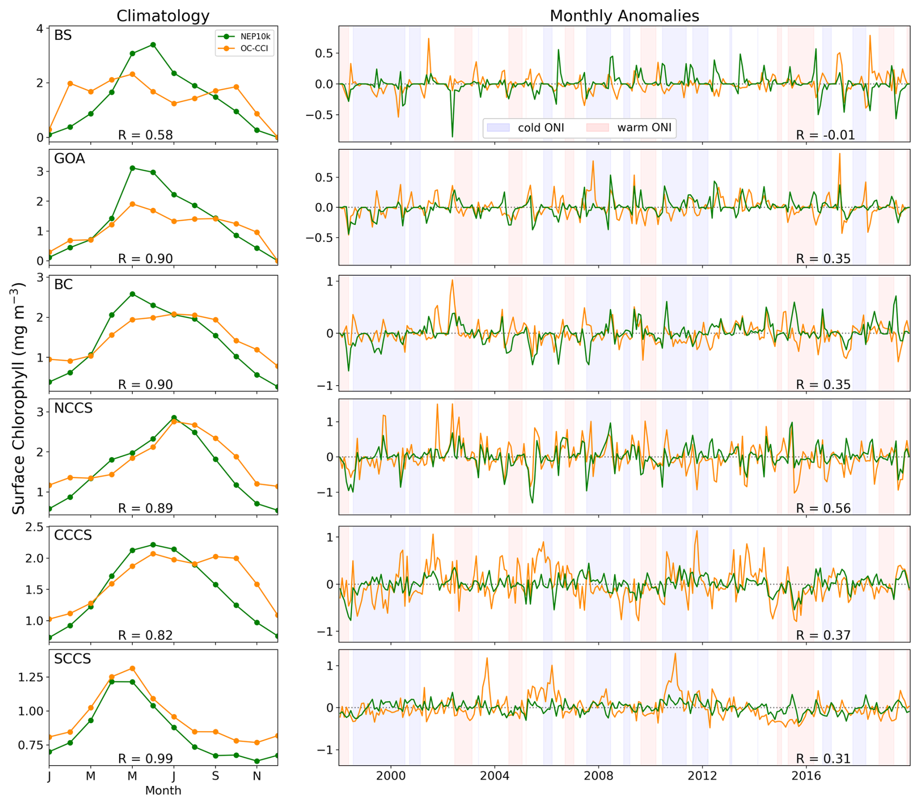
Figure 18Regional chlorophyll time series comparisons. Regional shelf (<500 m) surface chlorophyll monthly climatologies (left column) and anomaly time series (right column) for the satellite-derived OC-CCI product (orange) and NEP10k (green). Pearson correlation coefficients are reported for both climatologies and anomalies; background shading in the monthly anomaly time series plots indicates the oceanic Niño index produced by the NOAA Climate Prediction Center for context.
KGE for full chlorophyll time series are more moderate than those achieved for temperature, though only the GOA and the SCCS exhibit values below 0.6. For the GOA, this value was attributable to both the relative bias and variance, while in the SCCS, lower correlation and relative variance were the primary contributors to a lower KGE. Regional monthly anomaly time series for NEP10k chlorophyll were generally weakly correlated with OC-CCI (Fig. 18, right column), with most R values slightly below 0.4. While these correlations are significant (p<0.01), their modest values temper expectations for actionable chlorophyll forecasts. A possible exception is found in the northern California Current, where high correlation (R=0.58) provides some ground for optimism. Conversely, simulated and OC-CCI chlorophyll anomalies in the Bering Sea were uncorrelated (). We emphasize that interpretation of both NEP10k's correspondence and misfits in Fig. 18 must be moderated by uncertainties associated with the derivation of satellite-based ocean color products in coastal waters.
3.2.1 Bering-Sea-specific indicators
As discussed in Sect. 1, the eastern Bering Sea has one of the most prolific demersal/benthic fisheries in the world, and its ecosystem dynamics are strongly shaped by fluctuating seasonal sea ice. Compared to the trawl results, NEP10k trawl-equivalent bottom temperature (Fig. 19) in the Bering Sea tends to be biased slightly warm, particularly in the mid-shelf region that approximately corresponds with the area of maximum/minimum September ice edge extent reported by Wang et al. (2014). The model exhibits a modest cold bias, in contrast, on the inner shelf of the southeastern Bering Sea. The NEP10k model, however, robustly reproduces interannual variability of the cold pool area (CPA) indices, with the best performance at the higher temperature thresholds (Fig. 20). The model does tend to underrepresent the CPA delineated by the coldest threshold (water temperature °C; dark blue in Fig. 20). This is emphasized by a particularly low KGE (−0.111), which is due to a particularly low relative bias and high relative variance. KGE for the °C threshold is also low, similarly due to relative variance and bias. However, the correlation remains high across thresholds, and there is minimal bias at the higher thresholds (i.e., water temperature ≤1 or 2 °C; lighter blues in Fig. 20). Critically, the simulation captures the very small CPAs in recent years that have been linked to recent declines in the lucrative snow crab fishery (Szuwalski et al., 2023).
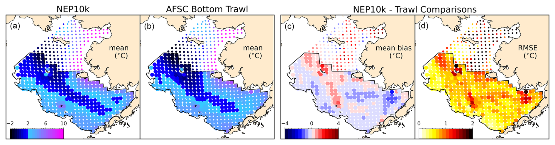
Figure 19Bering Sea cold pool extent. Comparison with AFSC Bering Sea summer trawl. Marker size is scaled by the number of annual data points that comprise the mean. The color map in a and b emphasizes the 2 °C transition point for consistency with the threshold value for identifying the cold pool. The black outline delineates the southeastern Bering Sea; trawl data collected from this region are used to calculate the Bering Sea summer cold pool extent and index.
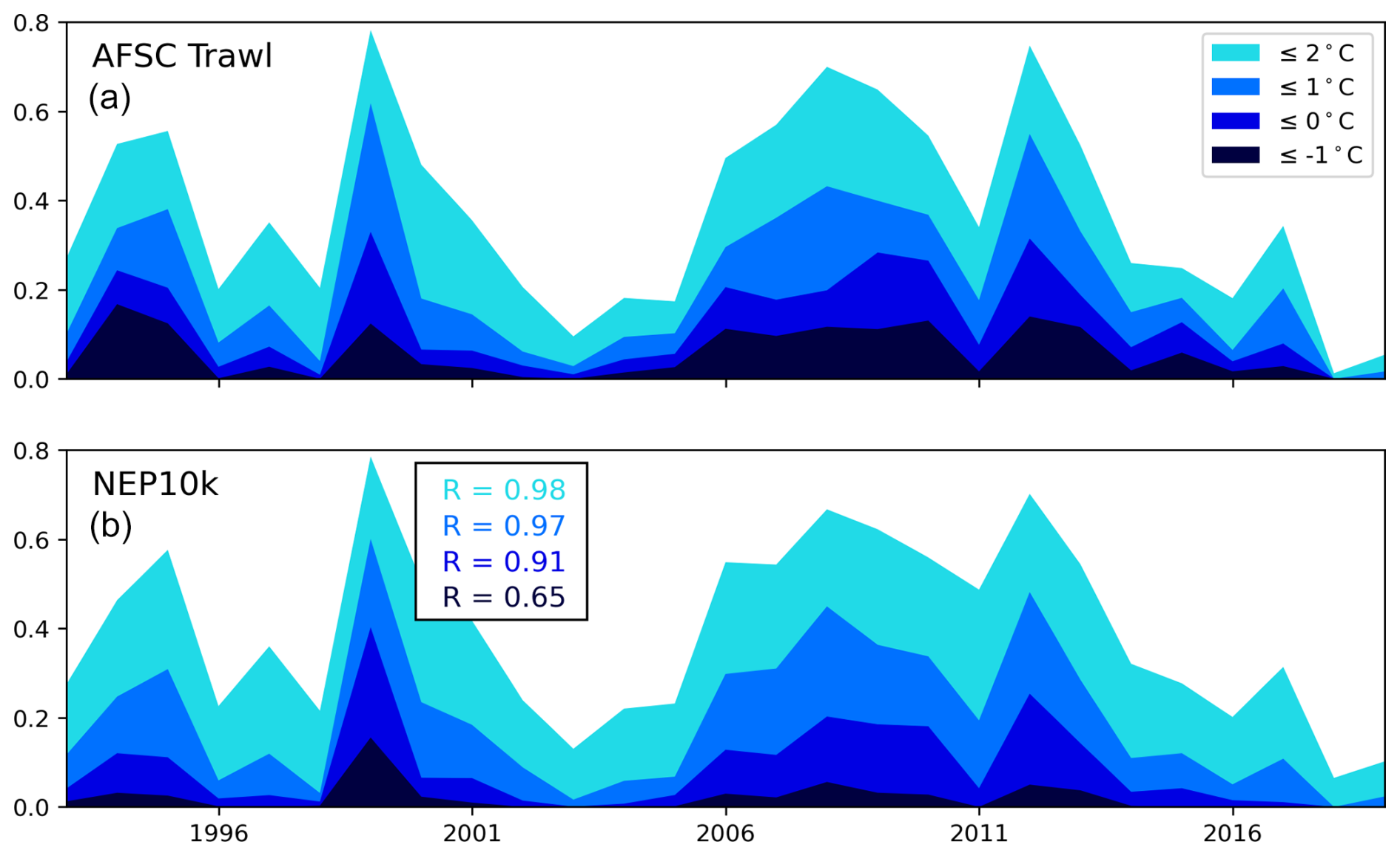
Figure 20Southeastern Bering Sea cold pool area index. Comparison of the cold pool index time series derived from the AFSC bottom trawl survey data (a) and the spatially and temporally consistent NEP10k bottom temperature output (b) following the methods described in Rohan et al. (2022) and the AFSC cold pool software repository. The plots report the fraction of the total survey of the southeastern Bering Sea trawl area (outlined in the figure above) that exhibits bottom temperatures under the specified thermal thresholds. We report Spearman correlation values between NEP10k and trawl indices in the bottom panel (b).
The NEP10k simulation does overestimate the sea ice concentration, particularly in the northern Bering Sea (Fig. 21). However, the contours for the 10 % and 50 % sea ice concentrations correspond with observations fairly well from January through April, suggesting that the simulation generates a reasonable spring sea ice extent. NEP10k ice extent time series for the southeastern Bering Sea (Fig. S16 in the Supplement) are highly correlated with the satellite product, though NEP10k does overestimate the coverage area, which may be consistent with the ∼0.5 °C Bering Sea cold bias noted in Fig. 2.
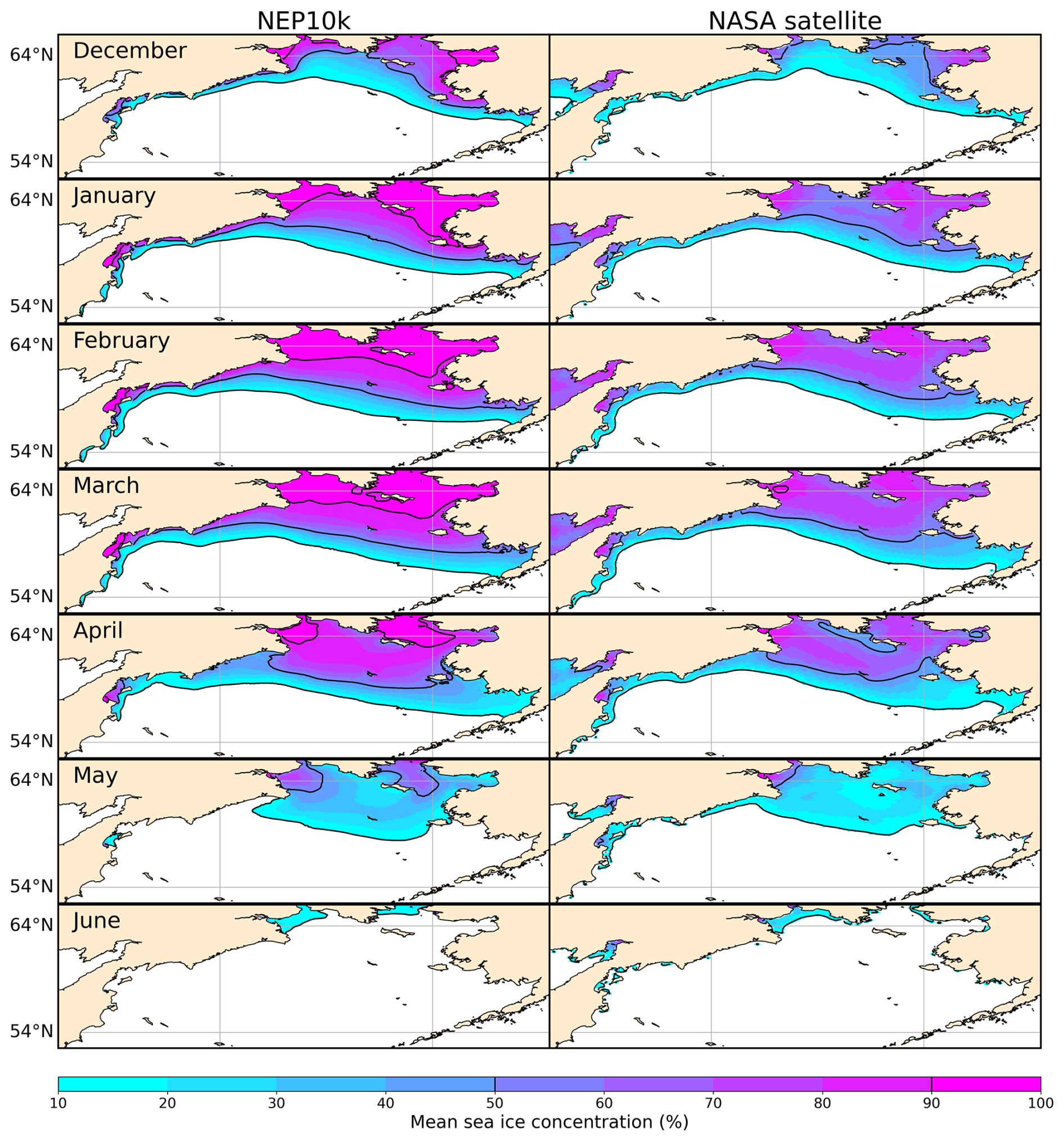
Figure 21Bering seasonal sea ice concentration and spatial extent. Comparison of spatial patterns in the Bering Sea monthly mean NEP10k sea ice concentration against NASA satellite estimates (Cavalieri et al., 1996). Black contours indicate the positions of the 10 % and 50 % sea ice concentrations.
3.2.2 Gulf-of-Alaska-specific indicators
NEP10k successfully simulates the two leading localized modes of SSH variability identified by Hauri et al. (2024) that can predispose the Gulf of Alaska to extreme physical and biogeochemical events (Fig. 22). The first two principal components (PCs) of the empirical orthogonal analysis of monthly NEP10k SSH in the Gulf of Alaska have spatial patterns that are consistent with the CMEMS SSH product, with significantly correlated spatial loading patterns in both cases (EOF1 R=4.2, EOF2 R=0.95; Fig. 22, top panels). The NEP10k-generated NGAO and GOADI time series are also in good agreement with satellite altimetry observed over the corresponding region and time frame, particularly at lower frequencies (Fig. 22, bottom panels). These two modes of variability comprise 47 % and 34 % of the variance in the model and observed SSH, respectively, suggesting that they may be somewhat overprominent in the model relative to other sources of SSH variability.
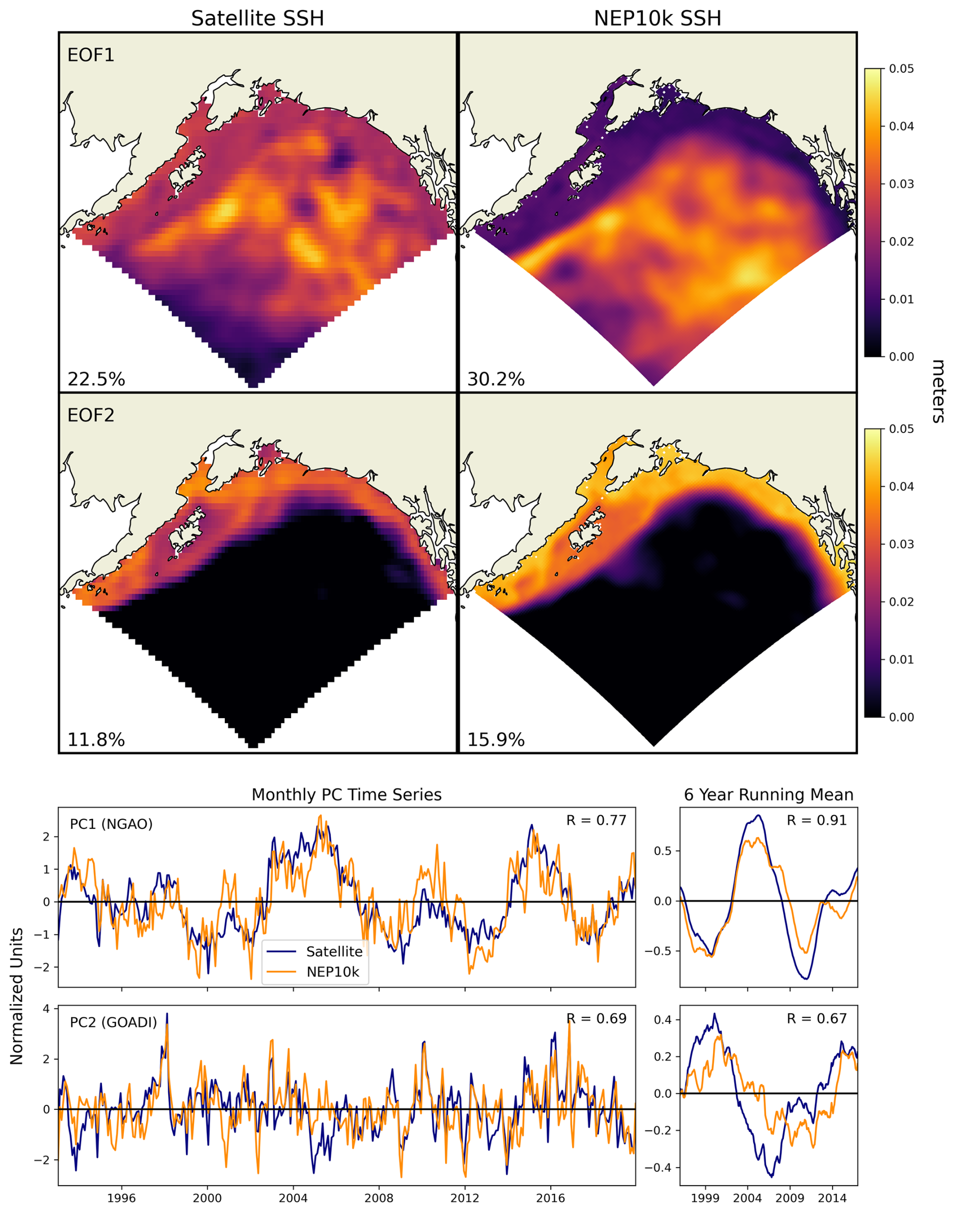
Figure 22GOA SSH EOFs and principal component time series. Spatial maps of the first (top row) and second (middle row) EOFs for satellite (left) and NEP10k (right) SSH variability. These are complemented with time series comparisons (monthly, left; 6-year running mean, right) for the first two principal components (NGAO, top row; GOADI, bottom row) from the empirical orthogonal function analyses of Gulf of Alaska sea surface height for NEP10k (orange) and the CMEMS satellite product (navy). R values indicate the Pearson correlation coefficient calculated between NEP10k and the satellite product, all of which are significant at p<0.001. X axis labels indicate 1 January of the specified year.
Composites of environmental conditions when the second PC, the GOADI, is below or above 1 demonstrate the impact of downwelling and relaxation of downwelling conditions, respectively, on shelf habitat in the Gulf of Alaska (Fig. 23). Relaxation of downwelling is associated with colder, lower-oxygen and more-acidic shelf waters from the enhanced intrusion of deep water. Conversely, positive phases of the GOADI exhibit significantly warmer bottom temperatures and elevated levels of bottom dissolved oxygen and aragonite saturation state.
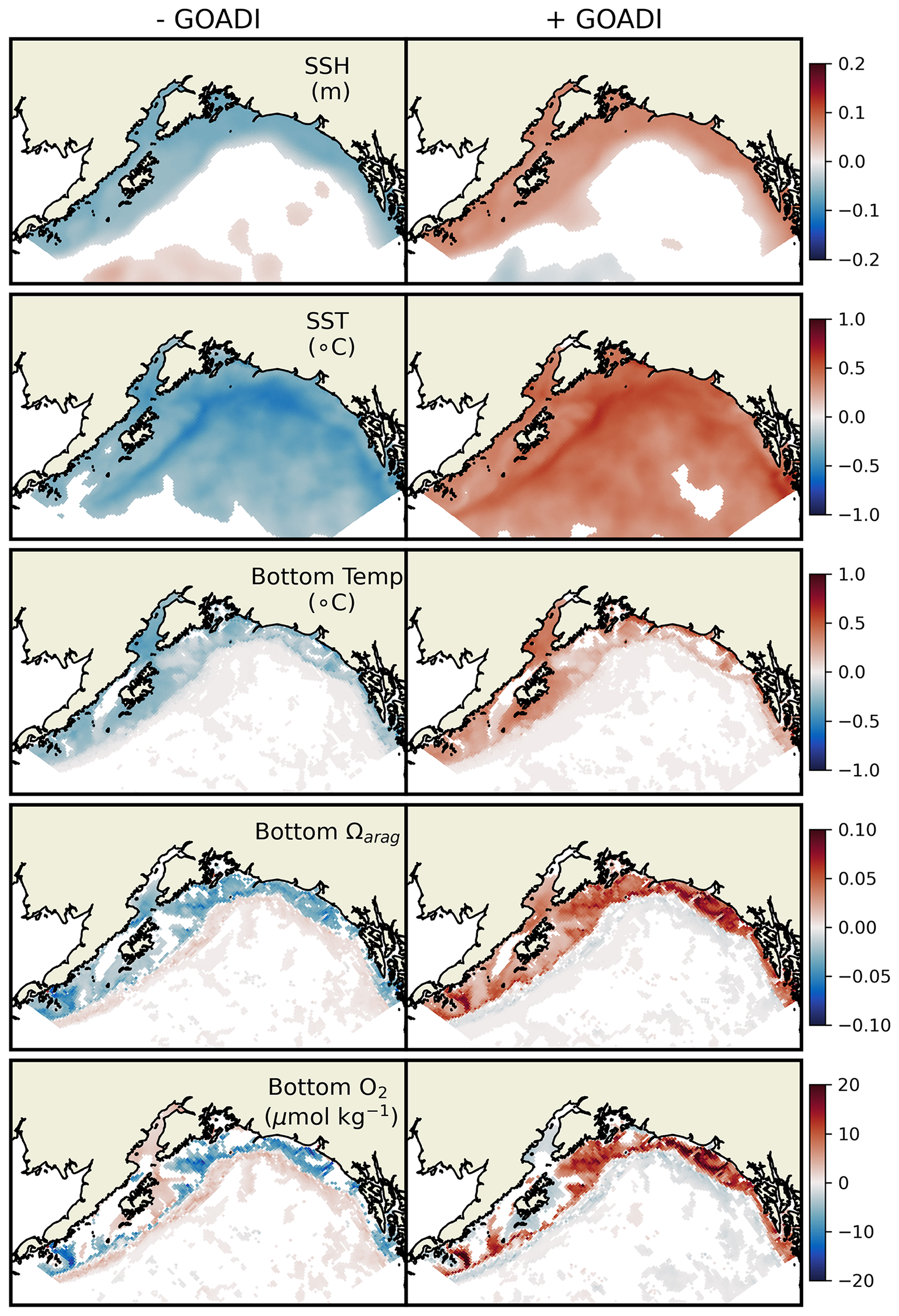
Figure 23GOADI composites. Composites of important ecological conditions during the positive (GOADI>1; 44 months out of 324) and the negative (; 45 months out of 324) phases of the Gulf of Alaska Downwelling Index (GOADI). Grid cells are colored where the composite differs significantly from 0 (student t-test, p<0.05).
3.2.3 California-Current-specific indicators
Seasonal upwelling plays an important role in CCS ecosystem dynamics, having bottom-up driving effects on primary productivity in this eastern boundary upwelling system (Sect. 1, Jacox et al., 2016). Summer upwelling conditions are evident in the map of vertical velocity (Fig. 24) with, on average, a predominantly positive/upward signal across the approximate mixed layer depth (30 m) from March through August, similar to that reported in Jacox et al. (2018). Monthly climatologies of NEP10k simulated vertical transport across 30 m demonstrate high correlation with the Jacox et al. (2018) CUTI metric, with R values above 0.92 at representative latitudes (Fig. 24). Correlations between the Jacox et al. (2018) monthly CUTI anomaly time series and corresponding NEP10k vertical transport are also significant, but the relationship is strongest at more northern latitudes (R=0.76 at 45° N) and drops off at more southerly latitudes (R=0.30 at 35° N). The 33N bin also exhibits the lowest KGE (0.248) for the full CUTI time series comparison, due to both a relatively low Pearson correlation coefficient and a fairly high relative variance. It is important to note, however, that the NEP10k and the ROMS model in Jacox et al. (2018) are forced by different atmospheric reanalysis products; thus, it may not be surprising that they differ in high-frequency variability. Additionally, the differences in methodologies such as approximating using a constant reference depth of 30 m for NEP10k could contribute to departures.
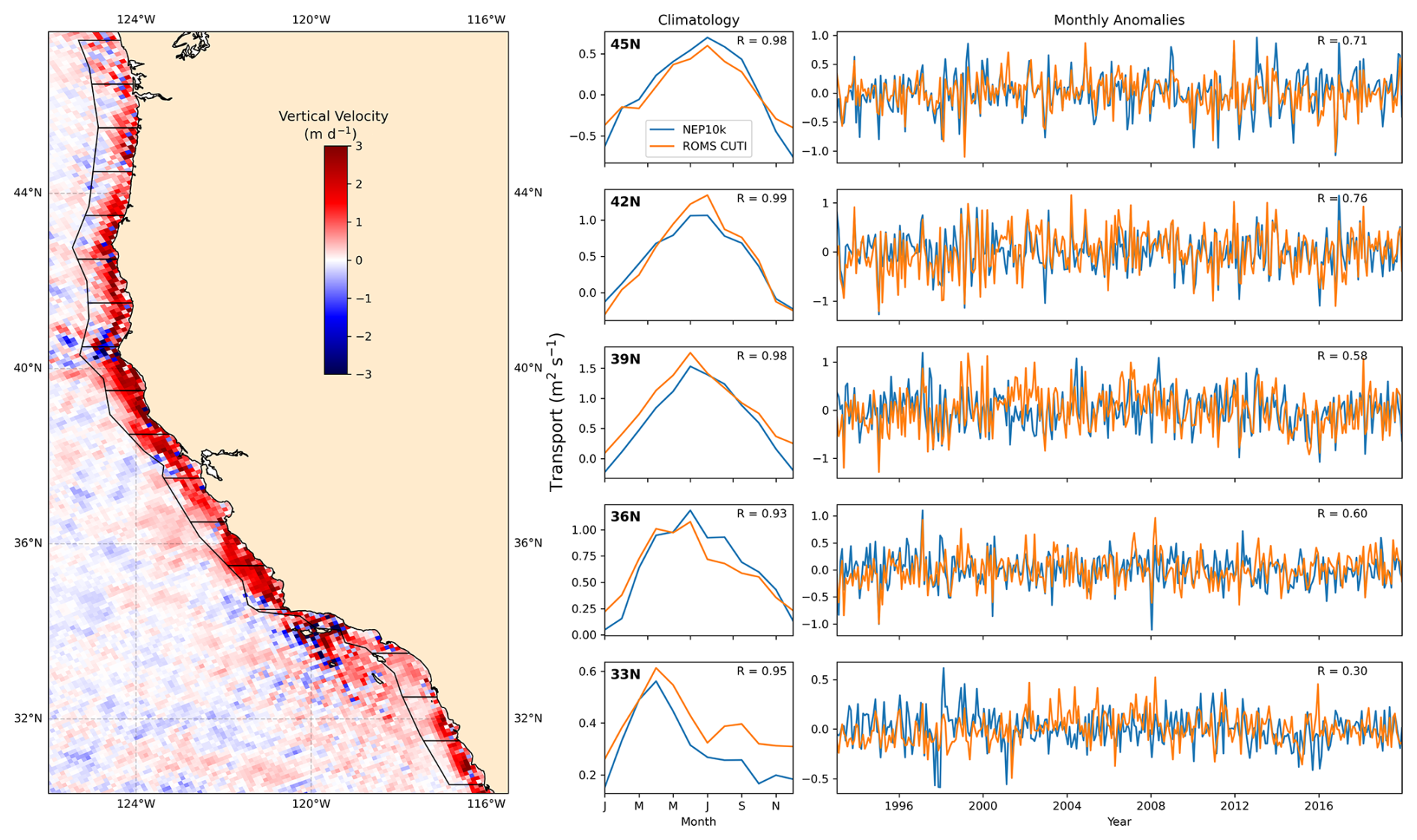
Figure 24CCS upwelling indices. Spring/summer (March–August) vertical velocity (map) at a depth of 30 m. Bins of 1° are indicated by the black outline and used for integrating vertical transport. This (blue line) is compared against the Jacox et al. (2018) ROMS CUTI metric (orange line) at several latitudes, decomposing the time series into monthly climatology (left) and anomalies (right). Pearson correlations (R) are reported in the upper-right corner of each time series panel; all correlations are significant (p<0.001).
NEP10k trends in dissolved oxygen reproduce offshore CalCOFI trends (Fig. 25), with strongest declines occurring at around 300 m and becoming less pronounced with depth. In the California Bight, however, NEP10k exhibits positive trends (most pronounced at a depth of 100 m) where the CalCOFI time series exhibit declining trends in dissolved oxygen levels. Many of the stations exhibiting discrepancies in the NEP10k are not statistically significant (p<0.05), and it should be noted that some of the time series are quite variable, with linear trends being sensitive to the time frame analyzed. Indeed, direct point-to-point comparisons against the CalCOFI bottle sample dataset (Figs. S26–S29 in the Supplement) demonstrate that, while NEP10k broadly reproduces temperature and salinity (Fig. S26, r≥0.89) and biogeochemistry (e.g., Fig. S27, r≥0.96) conditions in the southern California Current System, the model was more challenged to represent the temporal variation observed across decades for individual sampling sites and depth strata (Fig. S28). Agreement was best at the surface and for temperature but generally decreased with depth. Skill improved when values averaged across the CalCOFI sampling grid were considered (Fig. S29).
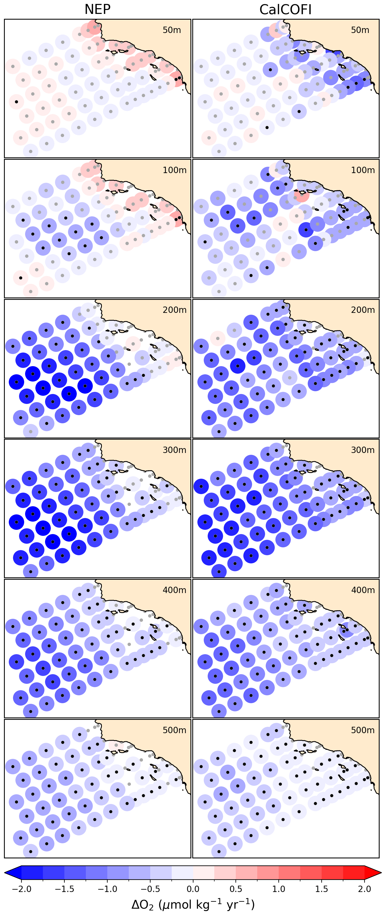
Figure 25CCS trends in dissolved oxygen at CalCOFI stations. Linear trends in subsurface dissolved oxygen (O2) at CalCOFI stations for NEP10k (left) and the CalCOFI dataset (right) calculated over the time frame of the NEP10k hindcast (1993–2019). Black markers indicate where station trends are significant (p<0.05), following Bograd et al. (2008).
3.3 Computational performance and scalability
As described in Sect. 1, the goal of the NEP10k configuration is to provide a simulation capable of skillfully resolving fisheries-critical features with manageable computational cost to allow for ensemble predictions and projections. Our baseline simulation averaged just over 5.3 h of wall clock time per hindcast year while distributing the 342×816 grid (cross-shore × along-shore) across a 32×80 decomposition (Fig. 26, green circle) and using a 400 s baroclinic time step and a 1200 s thermodynamic and tracer time step. After land masking, the run used 2036 PEs, yielding roughly 10 800 PE hours per simulation year on the c5 partition of NOAA's GAEA supercomputer. The 27-year hindcast produced herein thus requires ∼292 000 PE hours, while 1200 years of retrospective seasonal forecasts (e.g., Ross et al., 2024) would require approximately 13 million PE hours.
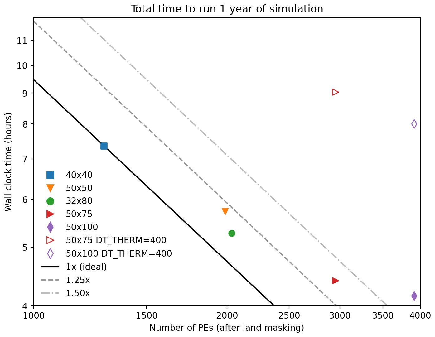
Figure 26Computational scalability efficiency. Amount of computer wall clock time used for completing 1 year of NEP10k simulation with a given number and configuration of processing elements (PEs). Markers indicate a given simulation's PE decomposition for diving in the horizontal model domain prior to omitting PEs that do not contain any ocean grid cells. The diagonal lines indicate constant computational cost (processes × time) relative to the 40×40 (blue square) reference simulation. The two hollow markers represent simulations wherein the thermodynamics time step was set to a dynamics time step (i.e., reduced from 1200 to 400).
The NEP10k computational cost is comparable to the recently published Northwest Atlantic regional MOM6 configuration (NWA12) of Ross et al. (2023), which used a 40×40 layout (1200 PEs after land masking) to generate 1 simulation year in about 9 h (about 10 800 PE hours per simulation year). While NWA12 was a larger domain, NEP10k required smaller baroclinic and thermodynamic time steps for stability (400 versus 600 s and 1200 versus 1800 s, respectively). The instability at longer time steps in the NEP10k configuration primarily occurred in the vicinity of the Aleutian island chain, where strong currents could be generated within tight channels.
Computational scaling tests showed that increases in throughput were achievable, but returns fell considerably below the ideal 1:1 scaling between the processor count and the wall clock time (Fig. 26). An approximate doubling of PEs from 2038 to nearly 4000, for example, only decreased the wall clock time for a simulation year from ∼5.3 to ∼4.2 h (compare the green circle and the purple diamond in Fig. 26). The decreased scaling is not unexpected, as higher processor counts decompose the model grid into increasingly granular tiles, taxing communication across PEs. This effect can also be seen when comparing the performance of the 32×80 baseline setting, which maximizes the number of interior to exterior cells on a PE by decomposing the 342×816 grid into squares, versus the approximately 10 % slower 50×50 decomposition that relies on rectangular elements. Scaling from the base configuration to lower processor counts, in contrast, is relatively strong, supporting the viability of running simulations on smaller supercomputing systems.
Consistent with the findings of Ross et al. (2023), we found considerable computational benefit from leveraging MOM6's capacity to have a longer thermodynamic and tracer time step than the baroclinic time step (closed versus open symbols in Fig. 26). Throughput was nearly doubled when the thermodynamics and tracer time step was 3 times longer than the baroclinic time step.
There were three primary design criteria for the NEP10k model. The first was that a coastwide configuration was needed to address coastwide challenges arising from climate change, such as shifting fisheries distributions across state and international boundaries. The second was that the model must resolve and accurately reproduce enough of the physical and biogeochemical drivers of ocean change in and across the disparate ecosystems within the domain to support ecosystem and fisheries applications. The third was that the model must be suited, both computationally and in terms of model skill, for ensemble predictions and projections. The comprehensive model evaluation herein suggests that the NEP10k configuration meets these design criteria sufficiently to provide a basis for initial applications and a robust foundation for further model improvement. The comparison against large-scale physical and biogeochemical patterns in Sect. 3.1 showed that a single physical–biogeochemical modeling framework could robustly capture the primary physical and biogeochemical contrasts between the EBS, GOA, and CCE (Figs. 2–5, 7–8, 12–15). Simulation fidelity extended to seasonal patterns in most quantities (Figs. 17 and 18, Figs. S1–S15) and robust matches to interannual variations for many, even within limited regions of the domain (Figs. 16, 19, 21, 24, and 25). While biases were present, and at times prominent, the skill achieved supports NEP10k's current utility. This discussion will focus on model characteristics contributing to successes and on further model developments that may ameliorate current limitations.
A central challenge for NEP10k was the representation of physical and biogeochemical processes governing a large range of ecosystems, from subtropical to polar and oligotrophic to eutrophic. Success in this regard requires model formulations and parameterizations that are robust across regimes. For ocean physics, one advance that led to notable improvement was the replacement of the submesoscale restratification parameterization of Fox-Kemper et al. (2011) with that of Bodner et al. (2023). The Fox-Kemper parameterization requires a single choice for the submesoscale front length, while Bodner diagnoses the front length from the ocean state, revealing considerable variability with season and latitude. Smaller front lengths at high latitudes proved critical to limiting deep mixing biases in the western Bering Sea, while longer front lengths further south were critical in limiting shallow mixed layer biases in the Gulf of Alaska and California Current (Fig. 4). Though the more dynamic Bodner scheme did not eliminate MLD biases, we did find that it improved them considerably relative to the Fox-Kemper et al. (2011) parameterization, where a single characteristic submesoscale frontal length scale forced one to exacerbate one bias or the other (Fig. S18 in the Supplement).
For biogeochemistry, starting with a model designed for global applications provided a sound starting point for achieving cross-system skill. Evaluation of the shelf-scale fidelity of global models, however, is generally limited by their often coarse resolution (e.g., Stock et al., 2014, 2020). A key addition to extend skill in NEP10k to coastal regions was an additional phytoplankton size class, which allowed the model to better resolve the coastal diatoms responsible for high chlorophyll concentrations along the coast. This expanded formulation was initially developed by Van Oostende et al. (2018) for use in the California Current, where it was shown to improve the resolution of both very high coastal chlorophyll concentrations and the biogeochemical signals that can be associated with them (e.g., coastal hypoxia). These benefits can be seen in the generally high coastal (relative to open ocean) chlorophyll levels along the U.S. West Coast (Fig. 10) and the robust depiction of the hypoxic boundary layer depth (Fig. 13). The most glaring chlorophyll bias is the model's tendency to underestimate winter/fall OC-CCI-estimated chlorophyll in the nearshore EBS (Fig. 10), which degrades the seasonal chlorophyll fidelity for this region (Fig. 18). Satellite-based estimates in shallow regions of the EBS actually peak during these months despite cold, dark, and vigorously mixed conditions, suggesting potential contamination of chlorophyll estimates in turbid coastal waters (Dierssen, 2010; Schofield et al., 2013). A recent study in the Arctic, for example, suggests that global satellite chlorophyll algorithms may overestimate chlorophyll by over a factor of 2 (Li et al., 2024).
Other chlorophyll and plankton misfits require additional scrutiny. The tendency to overestimate offshore spring and summer chlorophyll along the margin separating the Gulf of Alaska and the California Current, for example, may reflect biases in dust delivery, dust solubility, or iron scavenging in this iron-limited region. The relatively persistent and strong iron limitation in the offshore waters of the California Current in NEP10k, however, may already exceed the “mosaic” of alternating N and Fe limitation suggested by some prior studies (Messié and Chavez, 2015; Moore et al., 2013; Till et al., 2019). A spatially indiscriminate iron tuning is thus unlikely to resolve these biases. They may also arise, however, from misrepresented grazing controls. NEP10k's skill in simulating mesozooplankton biomass is limited to capturing first-order cross-ecosystem and seasonal biomass contrasts (Fig. 11), with the patchiness in mesozooplankton biomass in net tow data being underrepresented. There are also some systematic biases, such as the tendency for mesozooplankton populations to be displaced offshore and biased low relative to observations during the summer upwelling season in the California Current. Previous work (e.g., Batchelder et al., 2002) has suggested that zooplankton may enlist diurnal vertical migration to avoid being swept offshore, alternating between surface feeding in offshore currents at night and predator avoidance in inshore flowing currents during the day. Such behavior is not included in NEP10k but could increase mesozooplankton biomass and shift the distribution inshore.
Capturing mean spatial and seasonal patterns is a critical starting point for any model intended for ecosystem/fisheries science and management applications. Many applications, however, require the capacity to anticipate change across seasonal to multidecadal management time horizons (Tommasi et al., 2017). The robust representation of surface and bottom temperature variability (Fig. 16) provides a promising start in this regard. Temperature anomalies are a first-order indicator of ecosystem conditions and a primary determinant of habitat viability (e.g., Deutsch et al., 2015), and temperature extremes are a primary source of ecosystem stress in a changing climate (e.g., Frölicher et al., 2018). The robust representation of surface and bottom water anomalies at a regional scale and for shallower waters (<500 m), combined with the growing capacity of global prediction systems to anticipate fluctuations in large-scale climate drivers (e.g., ENSO), supports the potential viability of predictive applications. Retrospective forecast experiments are underway to assess this. NEP10k was less successful, however, in capturing coastal chlorophyll anomalies (Fig. 17). The correlation with monthly chlorophyll anomalies was only marginally significant in most systems, approaching useful levels (i.e., R∼0.6) in the NCCS. This weaker correlation was not necessarily surprising, given the volatile and patchy nature of coastal chlorophyll and observing challenges in such environments, but points to the need for further scrutiny of both the model and observations before predictive chlorophyll applications can be realized in most systems.
Possibly the most critical metrics for ecosystems and fisheries applications considered herein were the region-specific quantities considered in Figs. 18–25. These were drawn from existing management-linked documents, such as the “State of the Ecosystem” reports created by NOAA's National Marine Fisheries Service to strategically inform management decisions. Evaluations against the admittedly limited set of region-specific fisheries metrics herein was generally positive. Perhaps the most striking of these successes is the fidelity with which NEP10k reproduces the Bering Sea cold pool relative to over 2 decades of Alaska Fisheries Science Center bottom trawl data (Figs. 19 and 20). The model's representation of these metrics was improved during the course of development when an excess of shear-driven mixing on the Bering shelf was identified and addressed with an adjustment of Jackson et al. (2008) shear mixing parameterization. The addition of a simple scaling factor for the geometric limitation imposed by this formulation was found to be the most effective way to pragmatically calibrate the shear-driven mixing to better produce observed values for both mixing and bottom temperature. A more comprehensive analysis of this parameterization and its impact on Bering Sea dynamics is currently underway (Seelanki et al., 2025) and will inform regional MOM6 shear mixing parameterization for mixed turbulence regimes.
While NEP10k's overall representation of variations in the Bering Sea cold pool extent was excellent, the model did underestimate the summer extent of the coldest bottom water ( °C; darkest blue in Fig. 19). This seemingly conflicts with NEP10k's overrepresentation of seasonal sea ice extent (Figs. 20 and S16) because greater sea ice extent and coverage tend to be associated with a more extensive cold pool (e.g., Wyllie-Echeverria and Wooster, 1998). The model does achieve substantial winter levels of cold bottom water (Fig. S19 in the Supplement), but they erode more quickly than observed in May and June, just prior to the trawl season. This decline in bottom coverage by the coldest water mass category coincides with a dramatic monthly reduction in NEP10k's SEBS sea ice extent relative to satellite estimates (Fig. S20 in the Supplement, May–April and June–May). The drivers of this bias will be explored. We emphasize, however, that simulated Bering Sea ice variations in NEP10k are highly correlated with observations (Fig. S16), suggesting the potential for predictive applications despite the mean sea ice bias.
NEP10k reproduction of localized modes of low-frequency climate variability in the Gulf of Alaska (NGAO and GOADI, correlation with satellite-derived PCs >0.65, Fig. 22) holds promise for potential for multiyear to decadal fisheries applications in the GOA. These modes of variability map onto important ecosystem drivers such as bottom temperature and aragonite saturation state (Figs. 22 and S17 in the Supplement) and can contribute to extreme compound events that can have severe consequences for marine ecosystems (Hauri et al., 2024). Understanding of the relationships between SSH variability and shelf ecosystem conditions will be aided by the growing availability of physical and biogeochemical observations of GOA bottom conditions. Increasing the horizontal resolution of the NEP10k configuration may further improve representations of important regional GOA ecosystem features. For example, sea surface heights south of the Aleutian island chain, central to the Alaska Gyre, are lower than observed in reference datasets (Fig. 5) and could improve with better resolution of opposing horizontal flows, specifically the southwestward Alaska stream and eastward Subarctic or Aleutian Current. Higher resolution may also improve the representation of transports through the Aleutian island chain, which can significantly impact water mass properties in the Bering Sea (Stabeno et al., 1999).
Finally, in the California Current System, our regional assessment focused on ecosystem-critical seasonal upwelling and source water trends. NEP10k's climatological vertical transport at 30 m along the continental U.S. West Coast is highly correlated (i.e., R values≥0.93, Fig. 24) with the CUTI metric published by Jacox et al. (2018). Similarly, reproduction of multidecadal trends in dissolved O2 (Fig. 25) observed in the CalCOFI record was an important benchmark, indicative of the model's ability to capture processes driving ecologically consequential deoxygenation in the southern CCE (Bograd et al., 2008). While these findings further support the suitability of the current NEP10k configuration for ecological applications, continued model development will seek to understand and improve localized performance. For example, warm/cold-biased climatological surface/bottom temperatures in both CCCS and SCCS (Fig. 17), underrepresentation of climatological upwelling and low correlation in upwelling monthly anomalies (33N in Fig. 24), and underrepresentation of deoxygenation trends in the Southern California Bight (200 m and 300 m depths in Fig. 25) suggest that we may not be adequately representing the physical processes that influence these conditions due to excessive stratification in the southern CCE. Given the complex bathymetry and circulation that impact these processes in the Southern California Bight (e.g., Hickey, 1992), this is another instance where increased spatial resolution may improve model performance. Indeed, at a 10 km resolution, the SCCS shelf (where depth ≤500 m) extends as little as a single grid cell (or less) offshore. However, while higher-resolution (i.e., ∼5 km) simulations are currently underway, any benefits of doubling the horizontal resolution will need to be balanced against the roughly 8-fold increase in computational cost (i.e., 2-fold for each horizontal dimension and an additional 2-fold increase for the need to shorten the time step needed to maintain Courant–Friedrichs–Lewy stability). For applications wherein many-fold higher resolution is necessary, it may be more practical to utilize a smaller, higher-resolution nested domain (e.g., modeling the Salish Sea in Khangaonkar et al., 2018) that can be forced by the NEP10k at the open boundaries, rather than increasing the resolution for the full NEP10k domain. Continued NEP10k development will incorporate comparison against a broader array of local observation datasets similar to that of CalCOFI. Such extensive observation records are invaluable for better understanding and evaluating model performance, particularly in regions that may not be well represented in relatively coarse, gridded data products. However, it is important to approach such comparisons with realistic expectations. As shown in Fig. S28, NEP10k poorly reproduces temporal variability (i.e., low Pearson correlation coefficients) of repeated samplings of individual stations across multiple years. This is not surprising because the NEP10k hindcast does not assimilate observations, and thus any biases in the mean locations of fronts and other features are compounded by stochastic mesoscale and submesoscale features whose precise locations and timing will not match those observed. Indeed, more coherent patterns emerge after averaging over such features (e.g., Figs. S29, 17, and 20), which demonstrates that NEP10k's strength and utility are in representing reasonable approximations of ecologically important environmental conditions rather than an exact reproduction of in situ observations.
The results presented herein demonstrate that NEP10k is “fit for purpose” – in terms of both model skill and computation cost – for numerous living marine resource management applications across multiple time horizons. The model also establishes a basis for community evaluation to assess against a much broader set of fisheries and ecosystem metrics and a basis for co-development with fisheries scientists and managers to address identified limitations and maximize model utility. As part of NOAA's Changing Ecosystems and Fisheries Initiative, the community contributing to this effort has grown tremendously, facilitated by the open development of MOM6, COBALT, and preprocessing and analytical scripts made available via the CEFI GitHub. With increasing input from collaborators and co-development with end users, ongoing model development will prioritize NEP10k representation of key ecosystem indicators to maximize the utility of climate change projections and forecasts for living marine resource management.
Table A1Notable parameters, their current names, and the associated values used in the physical ocean (MOM6) component of the model and relevant references. BGC denotes biogeochemistry; SAL denotes self-attraction and loading. Bold text indicates where parameter choices differ from Ross et al. (2023). Comprehensive documentation of physical MOM6 parameters can be found in MOM_parameter_doc.all (Drenkard et al., 2024a).
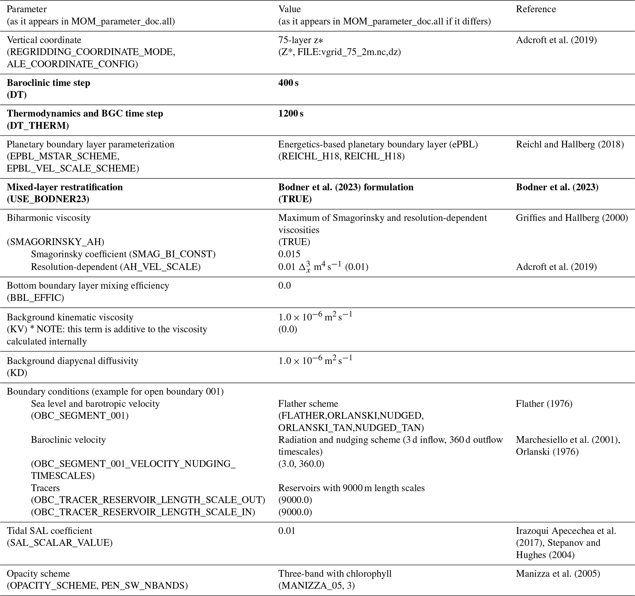
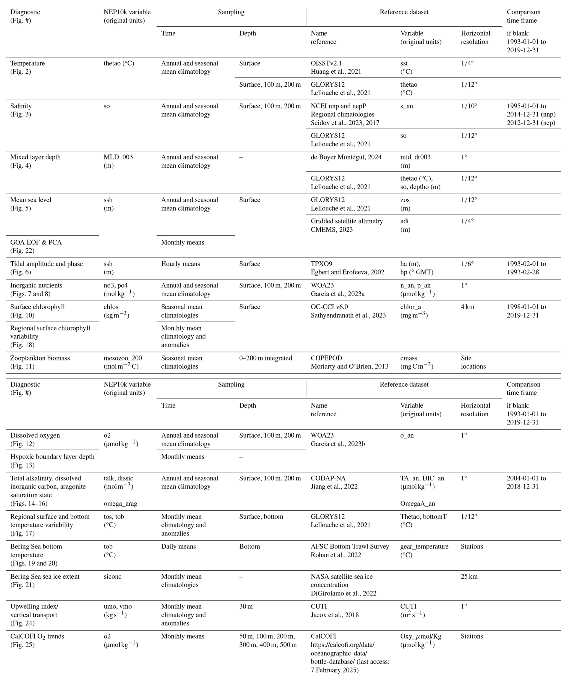
The source code for each component of the model has been archived at https://doi.org/10.5281/zenodo.13936294 (Drenkard et al., 2024c). The GitHub repositories for MOM6 can be found at https://github.com/mom-ocean/MOM6 (Modular Ocean Model, 2024) and https://github.com/NOAA-GFDL/MOM6 (NOAA-GFDL, 2024a). Repositories for other model components are also available at https://github.com/NOAA-GFDL (NOAA-GFDL, 2024b). Codes for generating regional MOM6 initial conditions, boundary conditions, and other necessary model inputs as well as diagnostic scripts are maintained on the NOAA CEFI GitHub repository: https://github.com/NOAA-GFDL/CEFI-regional-MOM6/ (NOAA-GFDL, 2024c). The Alaska Fisheries Science Center (AFSC) R code base used for the Bering Sea cold pool analyses can be found on GitHub at https://github.com/afsc-gap-products/coldpool (NOAA-AFSC, 2024a), which utilizes the AFSC akgfmaps toolset, also on GitHub at https://github.com/afsc-gap-products/akgfmaps (NOAA-AFSC, 2024b). Carter et al. (2021) alkalinity and DIC estimation algorithm (ESPER; https://doi.org/10.5281/zenodo.5512697, Carter, 2021).
All model output, the part that was analyzed, and the corresponding analysis codes used in preparing this paper have been published at https://doi.org/10.5281/zenodo.13936240 (Drenkard et al., 2024b). Model parameter, forcing, and initial condition files are published at https://doi.org/10.5281/zenodo.13936479 (Drenkard et al., 2024a). The datasets used for model validation and comparison, which are tabulated in Appendix Table 2, with the associated URL or DOI from which the data can be downloaded are as follows: OISSTv2.1 (https://www.ncei.noaa.gov/products/optimum-interpolation-sst, Huang et al., 2021); GLORYS12 reanalysis (https://doi.org/10.48670/moi-00021, Lellouche et al., 2021); NCEI Northern North Pacific Regional Climatology, version 2 (https://doi.org/10.25921/dym6-q737, Seidov et al., 2023); NCEI Northeast Pacific Regional Climatology (https://doi.org/10.7289/V5NC5ZDN; Seidov et al., 2017); de Boyer Montégut mixed layer depth over the global ocean (https://doi.org/10.17882/98226, de Boyer Montégut, 2024; de Boyer Montégut et al., 2004); Global Ocean Gridded L 4 Sea Surface Heights and Derived Variables (https://doi.org/10.48670/moi-00148; CMEMS, 2023); OSU TPXO9 Tide Model (https://www.tpxo.net/home, Egbert and Erofeeva, 2002); World Ocean Atlas 2023 Nitrate, Phosphate, and Oxygen Output (https://doi.org/10.25923/39qw-7j08, Garcia et al., 2023a; https://doi.org/10.25923/rb67-ns53, Garcia et al., 2023b); ESA Ocean Colour Climate Change Initiative (Ocean_Colour_cci): Global chlorophyll a data products gridded on a geographic projection at 4 km resolution, Version 6.0 (https://catalogue.ceda.ac.uk/uuid/b0ec72a28b6a4829a33ed9adc215d5bc/, Sathyendranath et al., 2019); COPEPOD-2012 (https://www.st.nmfs.noaa.gov/copepod/biomass/biomass-fields.html, Moriarty and O'Brien, 2013); CODAP-NA total alkalinity, DIC, and aragonite saturation (https://doi.org/10.25921/g8pb-zy76, https://www.ncei.noaa.gov/data/oceans/ncei/ocads/metadata/0270962.html, last access: 29 April 2023, Jiang et al., 2022); NOAA NCEP Ocean Niño Index (https://origin.cpc.ncep.noaa.gov/products/analysis_monitoring/ensostuff/detrend.nino34.ascii.txt, NOAA Climate Prediction Center, 2023b; AFSC bottom trawl gear temperature data (https://github.com/afsc-gap-products/coldpool/tree/main/data, Rohan et al., 2022; Rohan, 2025); NASA NSIDC Sea Ice Concentrations from Nimbus-7 SMMR and DMSP SSM/I-SSMIS Passive Microwave Data, Version 2 (https://doi.org/10.5067/MPYG15WAA4WX, DiGirolamo et al., 2022); Coastal Upwelling Transport Index (CUTI; https://oceanview.pfeg.noaa.gov/data/ui/CUTI_daily.csv, Jacox et al., 2018); and California Cooperative Oceanic Fisheries Investigations (CalCOFI) Bottle Database (https://calcofi.org/downloads/database/CalCOFI_Database_194903-202105_csv_16October2023.zip, National Marine Fisheries Service (NOAA) et al., 2025).
The datasets used to create the model forcing and the URL or DOI from which the data can be downloaded are as follows: GLORYS12 reanalysis (https://doi.org/10.48670/moi-00021, Lellouche et al., 2021); OSU TPXO9 Tide Model (https://www.tpxo.net/home, Egbert and Erofeeva, 2002); World Ocean Atlas (2018) (https://www.ncei.noaa.gov/archive/accession/NCEI-WOA18); GloFAS (https://doi.org/10.24381/cds.a4fdd6b9, Grimaldi et al., 2022); Coastal freshwater discharge simulations for the Gulf of Alaska, 1931–2021 (https://doi.org/10.24431/rw1k7d3, Beamer et al., 2016; Hill, 2023); ERA5 (https://doi.org/10.24381/cds.adbb2d47, Hersbach et al., 2023); RC4USCoast (https://doi.org/10.25921/9jfw-ph50, Gomez et al., 2022, 2023); Global River Chemistry database (GLORICH, https://doi.org/10.1594/PANGAEA.902360, Hartmann et al., 2019); Global NEWS 2 (https://ars.els-cdn.com/content/image/1-s2.0-S1364815210000186-mmc2.xls, Mayorga et al., 2010); ArcticGro (https://www.arcticgreatrivers.org/data, Holmes et al., 2012); Meinshausen et al. (2017) atmospheric CO2 (https://doi.org/10.22033/ESGF/input4MIPs.1118, Meinshausen and Vogel, 2016; https://doi.org/10.22033/ESGF/input4MIPs.9866, Meinshausen and Nicholls, 2018); and GFDL ESM4.1 model output prepared for CMIP6 CMIP historical (https://doi.org/10.22033/ESGF/CMIP6.8597, Krasting et al., 2018).
The supplement related to this article is available online at https://doi.org/10.5194/gmd-18-5245-2025-supplement.
ACR, CAS, AA, WC, RD, RH, KH, TC, and NZ contributed the source code for regional MOM6, COBALT, SIS2, and/or other components of the model framework. EJD, CAS, and ACR contributed to the preparation of the model input files. EJD, CAS, ACR, and EC contributed to the evaluation and interpretation of the model results. EJD and CAS prepared the initial draft of the paper. All coauthors participated in discussions during various stages of the model development and evaluation and read and approved the final version of the paper.
The contact author has declared that none of the authors has any competing interests.
Publisher's note: Copernicus Publications remains neutral with regard to jurisdictional claims made in the text, published maps, institutional affiliations, or any other geographical representation in this paper. While Copernicus Publications makes every effort to include appropriate place names, the final responsibility lies with the authors.
This paper is a contribution of NOAA's Changing Ecosystems and Fisheries Initiative. We extend our thanks to Gabriela Negrete and Matthew Harrison for their constructive feedback during the NOAA internal review process and to Samantha Siedlecki for contributions to ongoing regional MOM6 efforts. We also thank the two anonymous reviewers, who contributed comments that helped improve the paper.
Co-author Mercedes Pozo Buil was supported by the National Oceanic and Atmospheric Administration's Modeling, Analysis, Predictions, and Projections program (grant no. NA20OAR4310447) and co-authors Claudine Hauri and Rémi Pagès were supported by the North Pacific Research Board (grant no. NPRB 2109).
This paper was edited by Pearse Buchanan and reviewed by two anonymous referees.
Adcroft, A., and Campin, J.-M.: Rescaled height coordinates for accurate representation of free-surface flows in ocean circulation models, Ocean Model., 7, 269–284, https://doi.org/10.1016/j.ocemod.2003.09.003, 2004.
Adcroft, A., Anderson, W., Balaji, V., Blanton, C., Bushuk, M., Dufour, C. O., Dunne, J. P., Griffies, S. M., Hallberg, R., Harrison, M. J., Held, I. M., Jansen, M. F., John, J. G., Krasting, J. P., Langenhorst, A. R., Legg, S., Liang, Z., McHugh, C., Radhakrishnan, A., Reichl, B. G., Rosati, T., Samuels, B. L., Shao, A., Stouffer, R., Winton, M., Wittenberg, A. T., Xiang, B., Zadeh, N., and Zhang, R.: The GFDL global ocean and sea ice model OM4.0: Model description and simulation features, J. Adv. Model. Earth Sy., 11, 3167–3211, https://doi.org/10.1029/2019MS001726, 2019.
Alexander, M. A., Bladé, I., Newman, M., Lanzante, J. R., Lau, N., and Scott, J. D.: The Atmospheric Bridge: The Influence of ENSO Teleconnections on Air–Sea Interaction over the Global Oceans, J. Climate, 15, 2205–2231, https://doi.org/10.1175/1520-0442(2002)015<2205:TABTIO>2.0.CO;2, 2002.
Amaya, D. J., Alexander, M. A., Scott, J. D., and Jacox, M. G.: An evaluation of high-resolution ocean reanalyses in the California current system, Prog. Oceanogr., 210, 102951, https://doi.org/10.1016/j.pocean.2022.102951, 2023a.
Amaya, D. J., Jacox, M. G., Alexander, M. A., Scott, J. D., Deser, C., Capotondi, A., and Phillips, A. S.: Bottom marine heatwaves along the continental shelves of North America, Nat. Commun., 14, 1038, https://doi.org/10.1038/s41467-023-36567-0, 2023b.
Anderson, C. R., Moore, S. K., Tomlinson, M. C., Silke, J., and Cusack, C. K.: Living with harmful algal blooms in a changing world: strategies for modeling and mitigating their effects in coastal marine ecosystems, in: Coastal and Marine Hazards, Risks, and Disasters, edited by: Shroder, J. F., Ellis, J. T., and Sherman, D. J., Elsevier, 495–561, https://doi.org/10.1016/B978-0-12-396483-0.00017-0, 2015.
Anderson, C. R., Kudela, R. M., Kahru, M., Chao, Y., Rosenfeld, L. K., Bahr, F. L., Anderson, D. M., and Norris, T. A.: Initial skill assessment of the California Harmful Algae Risk Mapping (C-HARM) system, Harmful Algae, 59, 1–18, https://doi.org/10.1016/j.hal.2016.08.006, 2016.
Anderson, P. J. and Piatt, J. F.: Community reorganization in the Gulf of Alaska following ocean climate regime shift, Mar. Ecol. Prog. Ser., 189, 117–123, https://doi.org/10.3354/meps189117, 1999.
ArcticGro (The Arctic Great Rivers Observatory): Water Quality Dataset, Version 20240402, ArcticGro[data set], https://www.arcticgreatrivers.org/data (last access: 18 March 2025), 2024.
Bailey, K. M., Macklin, S. A., Reed, R. K., Brodeur, R. D., Ingraham, W. J., Piatt, J. F., Shima, M., Francis, R. C., Anderson, P. J., Royer, T. C., Hollowed, A., Somerton, D. A., and Wooster, W. S.: ENSO events in the northern Gulf of Alaska, and effects on selected marine fisheries, California Cooperative Oceanic Fisheries Investigations (CalCOFI) Report, 36, 78–96, https://pubs.usgs.gov/publication/2002017 (last access: 22 October 2024), 1995.
Batchelder, H. P., Edwards, C. A., and Powell, T. M.: Individual-based models of copepod populations in coastal upwelling regions: implications of physiologically and environmentally influenced diel vertical migration on demographic success and nearshore retention, Prog. Oceanogr., 53, 307–333, https://doi.org/10.1016/S0079-6611(02)00035-6, 2002.
Beamer, J. P., Hill, D. F., Arendt, A., and Liston, G. E.: High-resolution modeling of coastal freshwater discharge and glacier mass balance in the Gulf of Alaska watershed, Water Resour. Res., 52, 3888–3909, https://doi.org/10.1002/2015WR018457, 2016.
Bodner, A. S., Fox-Kemper, B., Johnson, L., Van Roekel, L. P., McWilliams, J. C., Sullivan, P. P., Hall, P. S., and Dong, J.: Modifying the Mixed Layer Eddy Parameterization to Include Frontogenesis Arrest by Boundary Layer Turbulence, J. Phys. Oceanogr., 53, 323–339, https://doi.org/10.1175/JPO-D-21-0297.1, 2023.
Bograd, S. J., Castro, C. G., Di Lorenzo, E., Palacios, D. M., Bailey, H., Gilly, W., and Chavez, F. P.: Oxygen declines and the shoaling of the hypoxic boundary in the California current: hypoxia in the California current, Geophys. Res. Lett., 35, L12607, https://doi.org/10.1029/2008GL034185, 2008.
Bograd, S. J., Schroeder, I., Sarkar, N., Qiu, X., Sydeman, W. J., and Schwing, F. B.: Phenology of coastal upwelling in the California Current, Geophys. Res. Lett., 36, L01602, https://doi.org/10.1029/2008GL035933, 2009.
Bograd, S. J., Jacox, M. G., Hazen, E. L., Lovecchio, E., Montes, I., Pozo Buil, M., Shannon, L. J., Sydeman, W. J., and Rykaczewski, R. R.: Climate change impacts on eastern boundary upwelling systems, Annu. Rev. Mar. Sci., 15, 303–328, https://doi.org/10.1146/annurev-marine-032122-021945, 2023.
Boyer, T. P., Garcia, H. E., Locarnini, R. A., Zweng, M. M., Mishonov, A. V., Reagan, J. R., Weathers, K. A., Baranova, O. K., Seidov, D., and Smolyar, I. V.: World Ocean Atlas 2018, NOAA National Centers for Environmental Information [data set], https://www.ncei.noaa.gov/archive/accession/NCEI-WOA18 (last access: 29 September 2020), 2019.
Briegleb, B. P. and Light, B.: A Delta-Eddington Multiple Scattering Parameterization for Solar Radiation in the Sea Ice Component of the Community Climate System Model (no. NCAR/TN-472+STR), University Corporation for Atmospheric Research, https://doi.org/10.5065/D6B27S71, 2007.
Brodie, S., Pozo Buil, M., Welch, H., Bograd, S. J., Hazen, E. L., Santora, J. A., Seary, R., Schroeder, I. D., and Jacox, M. G.: Ecological forecasts for marine resource management during climate extremes, Nat. Commun., 14, 7701, https://doi.org/10.1038/s41467-023-43188-0, 2023.
Brown, Z. W. and Arrigo, K. R.: Sea ice impacts on spring bloom dynamics and net primary production in the Eastern Bering Sea, J. Geophys. Res.-Oceans, 118, 43–62, https://doi.org/10.1029/2012JC008034, 2013.
Browning, T., Achterberg, E., Rapp, I., Engel, A., Bertrand, E. M., Tagliabue, A., and Moore, C. M.: Nutrient co-limitation at the boundary of an oceanic gyre, Nature, 551, 242–246, https://doi.org/10.1038/nature24063, 2017.
Browning, T. J. and Moore, C. M.: Global analysis of ocean phytoplankton nutrient limitation reveals high prevalence of co-limitation, Nat. Commun., 14, 5014, https://doi.org/10.1038/s41467-023-40774-0, 2023.
Byrne, R. H., Mecking, S., Feely, R. A., and Liu, X.: Direct observations of basin-wide acidification of the North Pacific Ocean, Geophys. Res. Lett., 37, L02601, https://doi.org/10.1029/2009GL040999, 2010.
Carter, B. R.: Empirical Seawater Property Estimation Routines, accepted, Zenodo [code], https://doi.org/10.5281/zenodo.5512697, 2021.
Carter, B. R., Bittig, H. C., Fassbender, A. J., Sharp, J. D., Takeshita, Y., Xu, Y.-Y., Álvarez, M., Wanninkhof, R., Feely, R. A., and Barbero, L.: New and updated global empirical seawater property estimation routines, Limnol. Oceanogr.-Meth., 19, 785–809, https://doi.org/10.1002/lom3.10461, 2021.
Cavalieri, D. J., Parkinson, C. L., Gloersen, P., and Zwally, H. J.: Sea Ice Concentrations from Nimbus-7 SMMR and DMSP SSM/I-SSMIS Passive Microwave Data, Version 1, National Snow and Ice Data Center [data set], https://doi.org/10.5067/8GQ8LZQVL0VL, 1996.
Chasco, B. E., Hunsicker, M. E., Jacobson, K. C., Welch, O. T., Morgan, C. A., Muhling, B. A., and Harding, J. A.: Evidence of Temperature-Driven Shifts in Market Squid Doryteuthis opalescens Densities and Distribution in the California Current Ecosystem, Mar. Coast. Fish., 14, e10190, https://doi.org/10.1002/mcf2.10190, 2022.
Cheng, W., Hermann, A. J., Coyle, K. O., Dobbins, E. L., Kachel, N. B., and Stabeno, P. J.: Macro- and micro-nutrient flux to a highly productive submarine bank in the Gulf of Alaska: A model-based analysis of daily and interannual variability, Prog. Oceanogr., 101, 63–77, https://doi.org/10.1016/j.pocean.2012.01.001, 2012.
Cheng, W., Curchitser, E., Stock, C., Hermann, A., Cokelet, E., Mordy, C., Stabeno, P., Hervieux, G., and Castruccio, F.: What processes contribute to the spring and fall bloom co-variability on the Eastern Bering Sea shelf?, Deep-Sea Res. Pt. II, 134, 128–140, https://doi.org/10.1016/j.dsr2.2015.07.009, 2015.
Christian, J. R. and Holmes, J.: Changes in albacore tuna habitat in the northeast Pacific Ocean under anthropogenic warming, Fish. Oceanogr., 25, 544–554, https://doi.org/10.1111/fog.12171, 2016.
Clement Kinney, J., Maslowski, W., Osinski, R., Lee, Y. J., Goethel, C., Frey, K., and Craig, A.: On the variability of the Bering Sea Cold Pool and implications for the biophysical environment, PLoS One, 17, e0266180, https://doi.org/10.1371/journal.pone.0266180, 2022.
Codiga, D. L.: Unified Tidal Analysis and Prediction Using the UTide Matlab Functions, Technical Report 2011-01, Graduate School of Oceanography, University of Rhode Island, Narragansett, RI, 59 pp., https://www.po.gso.uri.edu/~codiga/utide/2011Codiga-UTide-Report.pdf (last access: 23 November 2023), 2011.
Compton, T. J., Leathwick, J. R., and Inglis, G. J.: Thermogeography predicts the potential global range of the invasive European green crab (Carcinus maenas), Divers. Distrib., 16, 243–255, https://doi.org/10.1111/j.1472-4642.2010.00644.x, 2010.
Cordero-Quirós, N., Miller, A. J., Pan, Y., Balitaan, L., Curchitser, E., and Dussin, R.: Physical-Ecological Response of the California Current System to ENSO events in ROMS-NEMURO, Ocean Dynam., 72, 21–36, https://doi.org/10.1007/s10236-021-01490-9, 2022.
Coyle, K. O., Cheng, W., Hinckley, S. L., Lessard, E. J., Whitledge, T., Hermann, A. J., and Hedstrom, K.: Model and field observations of effects of circulation on the timing and magnitude of nitrate utilization and production on the northern Gulf of Alaska shelf, Prog. Oceanogr., 103, 16–41, https://doi.org/10.1016/j.pocean.2012.03.002, 2012.
Coyle, K. O., Hermann, A. J., and Hopcroft, R. R.: Modeled spatial-temporal distribution of productivity, chlorophyll, iron and nitrate on the northern Gulf of Alaska shelf relative to field observations, Deep-Sea Res. Pt. II, 165, 163–191, https://doi.org/10.1016/j.dsr2.2019.05.006, 2019.
Danielson, S., Curchitser, E., Hedstrom, K., Weingartner, T., and Stabeno, P.: On ocean and sea ice modes of variability in the Bering Sea, J. Geophys. Res., 116, C12034, https://doi.org/10.1029/2011JC007389, 2011.
Danielson, S. L., Hill, D. F., Hedstrom, K. S., Beamer, J., and Curchitser, E.: Demonstrating a high-resolution Gulf of Alaska ocean circulation model forced across the coastal interface by high-resolution terrestrial hydrological models, J. Geophys. Res.-Oceans, 125, e2019JC015724, https://doi.org/10.1029/2019JC015724, 2020.
de Baar, H. and de Jong, J.: Distributions, Sources and Sinks of Iron in Seawater, in: Biogeochemistry of Iron in Seawater, edited by: Turner, D. and Hunter, K. A., Wiley, New York, 123–253, ISBN 978-0-471-49068-5, 2001.
de Boyer Montégut, C.: Mixed layer depth over the global ocean: a climatology computed with a density threshold criterion of 0.03 kg m3 from the value at the reference depth of 5 m, SEANOE [data set], https://doi.org/10.17882/98226, 2024.
de Boyer Montégut, C., Madec, G., Fischer, A. S., Lazar, A., and Iudicone, D.: Mixed layer depth over the global ocean: an examination of profile data and a profile-based climatology, J. Geophys. Res., 109, C12003, https://doi.org/10.1029/2004JC002378, 2004.
Desmet, F., Gruber, N., Köhn, E. E., Münnich, M., and Vogt, M.: Tracking the space-time evolution of ocean acidification extremes in the California current system and northeast Pacific, J. Geophys. Res.-Oceans, 127, e2021JC018159, https://doi.org/10.1029/2021JC018159, 2022.
Desmet, F., Münnich, M., and Gruber, N.: Spatiotemporal heterogeneity in the increase in ocean acidity extremes in the northeastern Pacific, Biogeosciences, 20, 5151–5175, https://doi.org/10.5194/bg-20-5151-2023, 2023.
Deutsch, C., Ferrel, A., Seibel, B., Pörtner, H.-O., and Huey, R. B.: Climate change tightens a metabolic constraint on marine habitats, Science, 348, 1132–1135, https://doi.org/10.1126/science.aaa1605, 2015.
Di Lorenzo, E., Miller, E. J., Schneider, N., and McWilliams, J. C.: The Warming of the California Current System: Dynamics and Ecosystem Implications, J. Phys. Oceanogr., 35, 336–362, https://doi.org/10.1175/JPO-2690.1, 2005.
Di Lorenzo, E., Schneider, N., Cobb, K. M., Franks, P. J. S., Chhak, K., Miller, A. J., McWilliams, J. C., Bograd, S. J., Arango, H., Curchitser, E., Powell, T. M., and Rivière, P.: North Pacific Gyre Oscillation links ocean climate and ecosystem change, Geophys. Res. Lett., 35, L08607, https://doi.org/10.1029/2007GL032838, 2008.
Dierssen, H. M.: Perspectives on empirical approaches for ocean color remote sensing of chlorophyll in a changing climate, P. Natl. Acad. Sci. USA, 107, 17073–17078, https://doi.org/10.1073/pnas.0913800107, 2010.
DiGirolamo, N., Parkinson, C. L., Cavalieri, D. J., Gloersen, P., and Zwally, H. J.: Sea Ice Concentrations from Nimbus-7 SMMR and DMSP SSM/I-SSMIS Passive Microwave Data, Version 2, ASA National Snow and Ice Data Center Distributed Active Archive Center [data set], https://doi.org/10.5067/MPYG15WAA4WX, 2022.
Drenkard, E., Stock, C. A., Ross, A. C., Teng, Y.-C., Morrison, T., Cheng, W., Adcroft, A., Curchitser, E., Dussin, R., Hallberg, R., Hauri, C., Hedstrom, K., Hermann, A., Jacox, M. G., Kearney, K. A., Pages, R., Pilcher, D. J., Pozo Buil, M., Seelanki, V., and Zadeh, N.: Model input for initial submission of “A regional physical-biogeochemical ocean model for marine resource applications in the Northeast Pacific (MOM6-COBALT-NEP10k v1.0)” to GMD, Zenodo [data set], https://doi.org/10.5281/zenodo.13936479, 2024a.
Drenkard, E., Stock, C. A., Ross, A. C., Teng, Y.-C., Morrison, T., Cheng, W., Adcroft, A., Curchitser, E., Dussin, R., Hallberg, R., Hauri, C., Hedstrom, K., Hermann, A., Jacox, M. G., Kearney, K. A., Pages, R., Pilcher, D. J., Pozo Buil, M., Seelanki, V., and Zadeh, N.: Model output and analysis codes for initial submission of “A regional physical-biogeochemical ocean model for marine resource applications in the Northeast Pacific (MOM6-COBALT-NEP10k v1.0)” to GMD, Zenodo [data set], https://doi.org/10.5281/zenodo.13936240, 2024b.
Drenkard, E., Stock, C. A., Ross, A. C., Teng, Y.-C., Morrison, T., Cheng, W., Adcroft, A., Curchitser, E., Dussin, R., Hallberg, R., Hauri, C., Hedstrom, K., Hermann, A., Jacox, M. G., Kearney, K. A., Pages, R., Pilcher, D. J., Pozo Buil, M., Seelanki, V., and Zadeh, N.: Model source code for initial submission of “A regional physical-biogeochemical ocean model for marine resource applications in the Northeast Pacific (MOM6-COBALT-NEP10k v1.0)” to GMD, Zenodo [code], https://doi.org/10.5281/zenodo.13936294, 2024c.
Drenkard, E. J., Stock, C. A., Ross, A. C., Dixon, K. W., Adcroft, A., Alexander, M., Balaji, V., Bograd, S. J., Butenschön, M., Cheng, W., Curchitser, E., Di Lorenzo, E., Dussin, R., Haynie, A. C., Harrison, M., Hermann, A., Hollowed, A., Holsman, K., Holt, J., Jacox, M. G., Jang, C. J., Kearney, K. A., Muhling, B. A., Pozo Buil, M., Saba, V., Sandø, A. B., Tommasi, D., and Wang, M.: Next-generation regional ocean projections for living marine resource management in a changing climate, ICES J. Mar. Sci, 78, 1969–1987, https://doi.org/10.1093/icesjms/fsab100, 2021.
Deutsch, C., Frenzel, H., McWilliams, J. C., Renault, L., Kessouri, F., Howard, E., Liang, J.-H., Bianchi, D., and Yang, S.: Biogeochemical variability in the California Current System, Prog. Oceanogr., 196, 102565, https://doi.org/10.1016/j.pocean.2021.102565, 2021.
Dunne, J. P., Horowitz, L. W., Adcroft, A. J., Ginoux, P., Held, I. M., John, J. G., Krasting, J. P., Malyshev, S., Naik, V., Paulot, F., Shevliakova, E., Stock, C. A., Zadeh, N., Balaji, V., Blanton, C., Dunne, K. A., Dupuis, C., Durachta, J., Dussin, R., Gauthier, P. P. G., Griffies, S. M., Guo, H., Hallberg, R. W., Harrison, M., He, J., Hurlin, W., McHugh, C., Menzel, R., Milly, P. C. D., Nikonov, S., Paynter, D. J., Ploshay, J., Radhakrishnan, A., Rand, K., Reichl, B. G., Robinson, T., Schwarzkopf, D. M., Sentman, L. T., Underwood, S., Vahlenkamp, H., Winton, M., Wittenberg, A. T., Wyman, B., Zeng, Y., and Zhao, M.: The GFDL Earth System Model Version 4.1 (GFDL-ESM4.1): Overall Coupled Model Description and Simulation Characteristics, J. Adv. Model. Earth Sy., 12, e2019MS002015, https://doi.org/10.1029/2019MS002015, 2020.
Dussin, R., Curchitser, E. N., Stock, C. A., and Van Oostende, C. A.: Biogeochemical drivers of changing hypoxia in the California Current Ecosystem, Deep-Sea Res. Pt. II, 169–170, 104590, https://doi.org/10.1016/j.dsr2.2019.05.013, 2019.
Egbert, G. D. and Erofeeva, S. Y.: Efficient inverse modeling of barotropic ocean tides, J. Atmos. Ocean. Tech., 19, 183–204, https://doi.org/10.1175/1520-0426(2002)019<0183:EIMOBO>2.0.CO;2, 2002 (data available at: https://www.tpxo.net/home, last access: 23 November 2023).
E. U. Copernicus Marine Service Information (CMEMS): Global Ocean Gridded L 4 Sea Surface Heights And Derived Variables Reprocessed 1993 Ongoing, Marine Data Store [data set], https://doi.org/10.48670/moi-00148, 2023.
Evans, W., Mathis, J. T., and Cross, J. N.: Calcium carbonate corrosivity in an Alaskan inland sea, Biogeosciences, 11, 365–379, https://doi.org/10.5194/bg-11-365-2014, 2014.
Fabry, V. J., McClintock, J. B., Mathis, J. T., and Grebmeier, J. M.: Ocean acidification at high latitudes: the bellwether, Oceanography, 22, 160–171, https://www.jstor.org/stable/24861032 (last access: 22 October 2024), 2009.
Ferriss, B. E.: Ecosystem Status Report 2023: Gulf of Alaska, Stock Assessment and Fishery Evaluation Report, North Pacific Fishery Management Council, Anchorage, Alaska, USA, https://apps-afsc.fisheries.noaa.gov/REFM/docs/2023/GOAecosys.pdf (last access: 22 October 2024), 2023.
Flather, R.: A Tidal Model of the North-West European Continental Shelf, Mem. Soc. R. Sci. Liege., 10, 141–164, 1976.
Fox-Kemper, B., Danabasoglu, G., Ferrari, R., Griffies, S. M., Hallberg, R. W., Holland, M. M., Maltrud, M. E., Peacock, S., and Samuels, B. L.: Parameterization of mixed layer eddies. III: Implementation and impact in global ocean climate simulations, Ocean Model., 39, 61–78, https://doi.org/10.1016/j.ocemod.2010.09.002, 2011.
Frischknecht, M., Münnich, M., and Gruber, N.: Remote versus local influence of ENSO on the California Current System, J. Geophys. Res.-Oceans, 120, 1353–1374, https://doi.org/10.1002/2014JC010531, 2015.
Froelich, P. N.: Kinetic Control of Dissolved Phosphate in Natural Rivers and Estuaries: A Primer on the Phosphate Buffer Mechanism, Limnol. Oceanogr., 33, 649–668, https://doi.org/10.4319/lo.1988.33.4part2.0649, 1988.
Frölicher, T. L., Fischer, E. M., and Gruber, N.: Marine heatwaves under global warming, Nature, 560, 360–364, https://doi.org/10.1038/s41586-018-0383-9, 2018.
Galbraith, E. D., and Martiny, A. C.: A simple nutrient-dependence mechanism for predicting the stoichiometry of marine ecosystems, P. Natl. Acad. Sci. USA, 112, 8199–8204, https://doi.org/10.1073/pnas.1423917112, 2015.
García, H. E., Weathers, K., Paver, C. R., Smolyar, I., Boyer, T. P., Locarnini, R. A., Zweng, M. M., Mishonov, A. V., Baranova, O. K., Seidov, D., and Reagan, J. R.: World Ocean Atlas 2018, Volume 3: Dissolved Oxygen, Apparent Oxygen Utilization, and Oxygen Saturation, in: NOAA Atlas NESDIS 83, edited by: Mishonov, A., NOAA, 38 pp., https://doi.org/10.25923/qspr-pn52, 2019a.
García, H. E., Weathers, K., Paver, C. R., Smolyar, I., Boyer, T. P., Locarnini, R. A., Zweng, M. M., Mishonov, A. V., Baranova, O. K., Seidov, D., and Reagan, J. R.: World Ocean Atlas 2018, Volume 4: Dissolved Inorganic Nutrients (phosphate, nitrate and nitrate+nitrite, silicate), in: NOAA Atlas NESDIS 84, edited by: Mishonov, A., NOAA, 35 pp., https://doi.org/10.25923/ng6j-ey81, 2019b.
Garcia, H. E., Bouchard, C., Cross, S. L., Paver, C. R., Wang, Z., Reagan, J. R., Boyer, T. P., Locarnini, R. A., Mishonov, A. V., Baranova, O., Seidov, D., and Dukhovskoy, D.: World Ocean Atlas 2023, Volume 4: Dissolved Inorganic Nutrients (phosphate, nitrate, silicate), NOAA Atlas NESDIS 92 [data set], https://doi.org/10.25923/39qw-7j08, 2023a.
Garcia, H. E., Wang, Z., Bouchard, C., Cross, S. L., Paver, C. R., Reagan, J. R., Boyer, T. P., Locarnini, R. A., Mishonov, A. V., Baranova, O., Seidov, D., and Dukhovskoy, D.: World Ocean Atlas 2023, Volume 3: Dissolved Oxygen, Apparent Oxygen Utilization, and Oxygen Saturation, NOAA Atlas NESDIS 91 [data set], https://doi.org/10.25923/rb67-ns53, 2023b.
GEBCO Bathymetric Compilation Group: The GEBCO_2020 Grid – a continuous terrain model of the global oceans and land, British Oceanographic Data Centre, National Oceanography Centre, NERC [data set], https://doi.org/10.5285/a29c5465-b138-234d-e053-6c86abc040b9, 2020.
Gomez, F. A., Lee, S.-K., Stock, C. A., Ross, A. C., Resplandy, L., Siedlecki, S. A., Tagklis, F., and Salisbury, J. E.: RC4USCoast: A river chemistry dataset for regional ocean model application in the U.S. East, Gulf of Mexico, and West Coasts from 1950-01-01 to 2022-12-31 (NCEI Accession 0260455), NOAA National Centers for Environmental Information [data set], https://doi.org/10.25921/9jfw-ph50, 2022.
Gomez, F. A., Lee, S.-K., Stock, C. A., Ross, A. C., Resplandy, L., Siedlecki, S. A., Tagklis, F., and Salisbury, J. E.: RC4USCoast: a river chemistry dataset for regional ocean model applications in the US East Coast, Gulf of Mexico, and US West Coast, Earth Syst. Sci. Data, 15, 2223–2234, https://doi.org/10.5194/essd-15-2223-2023, 2023.
Griffies, S. M. and Hallberg, R. W.: Biharmonic Frictionwith a Smagorinsky-Like Viscosity for Use in LargeScale Eddy-Permitting Ocean Models, Mon. Weather Rev., 128, 2935–2946, https://doi.org/10.1175/1520-0493(2000)128<2935:BFWASL>2.0.CO;2, 2000.
Grimaldi, S., Salamon, P., Disperati, J., Zsoter, E., Russo, C., Ramos, A., Carton De Wiart, C., Barnard, C., Hansford, E., Gomes, G., and Prudhomme, C.: River discharge and related historical data from the Global Flood Awareness System, v4.0, European Commission, Joint Research Centre (JRC) [data set], https://doi.org/10.24381/cds.a4fdd6b9, 2022.
Grosholz, E. D., Ruiz, G. M., Dean, C. A., Shirley, K. A., Maron, J. L., and Connors, P. G.: The impacts of a nonindigenous marine predator in a California bay, Ecology, 81, 1206–1224, https://doi.org/10.1890/0012-9658(2000)081[1206:TIOANM]2.0.CO;2, 2000.
Gruber, N.: Warming up, turning sour, losing breath: ocean biogeochemistry under global change, Philos. T. Roy. Soc. A, 369, 1980–1996, https://doi.org/10.1098/rsta.2011.0003, 2011.
Gruber, N., Frenzel, H., Doney, S. C., Marchesiello, P., McWilliams, J. C., Moisan, J. R., Oram, J. J., Plattner, G.-K., and Stolzenbach, K. D.: Eddy-resolving simulation of plankton ecosystem dynamics in the California Current System, Deep-Sea Res. Pt. II, 53, 1483–1516, https://doi.org/10.1016/j.dsr.2006.06.005, 2006.
Gruber, N., Hauri, C., Lachkar, Z., Loher, D., Froelicher, T. L., and Plattner, G.-K.: Rapid progression of ocean acidification in the California Current System, Science, 337, 220–223, https://doi.org/10.1126/science.1216773, 2012.
Gupta, H. V., Kling, H., Yilmaz, K. K., and Martinez, G. F.: Decomposition of the mean squared error and NSE performance criteria: Implications for improving hydrological modelling, J. Hydrol., 377, 80–91, https://doi.org/10.1016/j.jhydrol.2009.08.003, 2009.
Hallberg, R.: Stable Split Time Stepping Schemes for Large-Scale Ocean Modeling, J. Comput. Phys., 135, 54–65, https://doi.org/10.1006/jcph.1997.5734, 1997.
Hallberg, R. and Adcroft, A.: Reconciling estimates of the free surface height in Lagrangian vertical coordinate ocean models with mode-split time stepping, Ocean Model., 29, 15–26, https://doi.org/10.1016/j.ocemod.2009.02.008, 2009.
Halpern, B. S., Kappel, C. V., Selkoe, K. A., Micheli, F., Ebert, C. M., Kontgis, C., Crain, C. M., Martone, R. G., Shearer, C., and Teck, S. J.: Mapping cumulative human impacts to California Current marine ecosystems, Conserv. Lett., 2, 138–148, https://doi.org/10.1111/j.1755-263X.2009.00058.x, 2009.
Hare, S. R. and Mantua, N. J.: Empirical evidence for North Pacific regime shifts in 1977 and 1989, Prog. Oceanogr., 47, 103–145, https://doi.org/10.1016/S0079-6611(00)00033-1, 2000.
Harrigan, S., Zsoter, E., Alfieri, L., Prudhomme, C., Salamon, P., Wetterhall, F., Barnard, C., Cloke, H., and Pappenberger, F.: GloFAS-ERA5 operational global river discharge reanalysis 1979–present, Earth Syst. Sci. Data, 12, 2043–2060, https://doi.org/10.5194/essd-12-2043-2020, 2020.
Hartmann, J., Lauerwald, R., and Moosdorf, N.: A Brief Overview of the GLObal RIver Chemistry Database, GLORICH, Proced. Earth Plan. Sc., 10, 23–27, https://doi.org/10.1016/j.proeps.2014.08.005, 2014.
Hartmann, J., Lauerwald, R., and Moosdorf, N.: GLORICH – Global river chemistry database, PANGAEA [data set], https://doi.org/10.1594/PANGAEA.902360, 2019.
Hauri, C., Gruber, N., Plattner, G.-K., Alin, S., Feely, R. A., Hales, B., and Wheeler, P. A.: Ocean acidification in the California Current system, Oceanography, 22, 60–71, 2009.
Hauri, C., Schultz, C., Hedstrom, K., Danielson, S., Irving, B., Doney, S. C., Dussin, R., Curchitser, E. N., Hill, D. F., and Stock, C. A.: A regional hindcast model simulating ecosystem dynamics, inorganic carbon chemistry, and ocean acidification in the Gulf of Alaska, Biogeosciences, 17, 3837–3857, https://doi.org/10.5194/bg-17-3837-2020, 2020.
Hauri, C., Pagès, R., McDonnell, A. M. P., Stuecker, M. F., Danielson, S. L., Hedstrom, K., Irving, B., Schultz, C., and Doney, S. C.: Modulation of ocean acidification by decadal climate variability in the Gulf of Alaska, Nat. Commun. Earth Env., 2, 191, https://doi.org/10.1038/s43247-021-00254-z, 2021.
Hauri, C., Pagès, R., Hedstrom, K., Doney, S. C., Dupont, S., Ferriss, B., and Stuecker, M. F.: More than marine heatwaves: A new regime of heat, acidity, and low oxygen compound extreme events in the Gulf of Alaska, AGU Adv., 5, e2023AV001039, https://doi.org/10.1029/2023AV001039, 2024.
Hermann, A. J., Hinckley, S., Dobbins, E. L., Haidvogel, D. B., Bond, N. A., Mordy, C., Kachel, N., and Stabeno, P. J.: Quantifying cross-shelf and vertical nutrient flux in the Coastal Gulf of Alaska with a spatially nested, coupled biophysical model, Deep-Sea Res. Pt. II, 56, 2474–2486, https://doi.org/10.1016/j.dsr2.2009.02.008, 2009.
Hermann, A. J., Gibson, G. A., Bond, N. A., Curchitser, E. N., Hedstrom, K., Cheng, W., Wang, M., Stabeno, P. J., Eisner, L., and Cieciel, K. D.: A multivariate analysis of observed and modeled biophysical variability on the Bering Sea shelf: Multidecadal hindcasts (1970–2009) and forecasts (2010–2040), Deep-Sea Res. Pt. II, 94, 121–139, https://doi.org/10.1016/j.dsr2.2013.04.007, 2013.
Hermann, A. J., Gibson, G. A., Bond, N. A., Curchitser, E. N., Hedstrom, K., Cheng, W., Wang, M., Hollowed, A. B., and Holsman, K. K.: Projected future biophysical states of the Bering Sea, Deep-Sea Res. Pt. II, 134, 30–47, https://doi.org/10.1093/icesjms/fsz043, 2016.
Hersbach, H., Bell, B., Berrisford, P., Hirahara, S., Horányi, A., Muñoz-Sabater, J., Nicolas, J., Peubey, C., Radu, R., Schepers, D., Simmons, A., Soci, C., Abdalla, S., Abellan, X., Balsamo, G., Bechtold, P., Biavati, G., Bidlot, J., Bonavita, M., De Chiara, G., Dahlgren, P., Dee, D., Diamantakis, M., Dragani, R., Flemming, J., Forbes, R., Fuentes, M., Geer, A., Haimberger, L., Healy, S., Hogan, R. J., Hólm, E., Janisková, M., Keeley, S., Laloyaux, P., Lopez, P., Lupu, C., Radnoti, G., de Rosnay, P., Rozum, I., Vamborg, F., Villaume, S., and Thépaut, J.-N.: The ERA5 global reanalysis, Q. J. Roy. Meteor. Soc., 146, 1999–2049, https://doi.org/10.1002/qj.3803, 2020.
Hersbach, H., Bell, B., Berrisford, P., Biavati, G., Horányi, A., Muñoz Sabater, J., Nicolas, J., Peubey, C., Radu, R., Rozum, I., Schepers, D., Simmons, A., Soci, C., Dee, D., and Thépaut, J.-N.: ERA5 hourly data on single levels from 1940 to present, Copernicus Climate Change Service (C3S) Climate Data Store (CDS) [data set], https://doi.org/10.24381/cds.adbb2d47, 2023.
Hibler, W. D.: A dynamic thermodynamic sea ice model, J. Phys. Oceanogr., 9, 815–846, https://doi.org/10.1175/1520-0485(1979)009<0815:ADTSIM>2.0.CO;2, 1979.
Hickey, B. M.: Circulation over the Santa Monica-San Pedro Basin and Shelf, Prog. Oceanogr., 30, 37–115, https://doi.org/10.1016/0079-6611(92)90009-O, 1992.
Hill, A. E., Hickey, B. M., Shillington, F. A., Strub, P., Brink, K. H., Barton, E. D., and Thomas, A. C.: Eastern ocean boundaries, in: The Sea, Vol. 11, The Global Coastal Ocean: Regional Studies and Syntheses, edited by: Robinson, A. R. and Brink, K. H., New York, John Wiley and Sons, Inc., 29–68, ISBN 0-471-11545-2, 1998.
Hill, D.: Coastal freshwater discharge simulations fo the Gulf of Alaska, 1931–2021, Research Workspace [data set], https://doi.org/10.24431/rw1k7d3, 2023.
Hill, C., DeLuca, C., Balaji, V., Suarez, M., and Da Silva, A.: The architecture of the earth system modeling framework, Comput. Sci. Eng., 6, 18, https://doi.org/10.1109/MCISE.2004.1255817, 2004.
Hinckley, S., Coyle, K. O., Gibson, G., Hermann, A. J., and Dobbins, E. L.: A biophysical NPZ model with iron for the Gulf of Alaska: Reproducing the differences between an oceanic HNLC ecosystem and a classical northern temperate shelf ecosystem, Deep-Sea Res. Pt. II, 56, 2520–2536, https://doi.org/10.1016/j.dsr2.2009.03.003, 2009.
Hollowed, A. B., Holsman, K. K., Wise, S. P., Haynie, A. C., Cheng, W., Evans, D. C. K., Hermann, A. J., Ianelli, J. N., Kearney, K. A., Punt, A. E., Reum, J. C. P., Stram, D. L., and Szuwalski, C. S.: Development of climate informed management scenarios for fisheries in the eastern Bering Sea, ICES J. Mar. Sci., 84, fsae034, https://doi.org/10.1093/icesjms/fsae034, 2024.
Holmes, R. M., Coe, M. T., Fiske, G. J., Gurtovaya, T., McClelland, J. W., Shiklomanov, A. I., Spencer, R. G. M., Tank, S. E., and Zhulidov, A. V.: Climate Change Impacts on the Hydrology and Biogeochemistry of Arctic Rivers, in: Climatic Change and Global Warming of Inland Waters, edited by: Goldman, C. R., Kumagai, M., and Robarts, R. D., John Wiley and Sons, Ltd., 1–26, https://doi.org/10.1002/9781118470596.ch1, 2012.
Holsman, K. K., Aydin, K., Sullivan, J., Hurst, T., and Kruse, G. H.: Climate effects and bottom-up controls on growth and size-at-age of Pacific halibut (Hippoglossus stenolepis) in Alaska (USA), Fish Oceanogr., 28, 345–358, https://doi.org/10.1111/fog.12416, 2019.
Holsman, K. K., Haynie, A. C., Hollowed, A. B., Reum, J. C. P., Aydin, K., Hermann, A. J., Cheng, W., Faig, A., Ianelli, J. N., Kearney, K. A., and Punt, A.: Ecosystem-based fisheries management forestalls climate-driven collapse, Nat. Commun., 11, 4579, https://doi.org/10.1038/s41467-020-18300-3, 2020.
Howard, E. M., Frenzel, H., Kessouri, F., Renault, L., Bianchi, D., McWilliams, J. C., and Deutsch, C.: Attributing causes of future climate change in the California Current System with multimodel downscaling, Global Biogeochem. Cy., 34, e2020GB006646, https://doi.org/10.1029/2020GB006646, 2020.
Huang, B., Liu, C., Banzon, V., Freeman, E., Graham, G., Hankins, B., Smith, T., and Zhang, H.-M.: Improvements of the Daily Optimum Interpolation Sea Surface Temperature (DOISST) Version 2.1, J. Climate, 34, 2923–2939, https://doi.org/10.1175/JCLI-D-20-0166.1, 2021 (data available at: https://www.ncei.noaa.gov/products/optimum-interpolation-sst last access: 26 June 2023).
Hughes, B. B., Levey, M. D., Fountain, M. C., Carlisle, A. B., Chavez, F. P., and Gleason, M. G.: Climate mediates hypoxic stress on fish diversity and nursery function at the land–sea interface, P. Natl. Acad. Sci. USA, 112, 8025–8030, https://doi.org/10.1073/pnas.1505815112, 2015.
Hunt Jr., G. L., Stabeno, P., Walters, G., Sinclair, E., Brodeur, R. D., Napp, J. M., and Bond, N. A.: Climate change and control of the southeastern Bering Sea pelagic ecosystem, Deep-Sea Res. Pt. II, 49, 5821–5853, https://doi.org/10.1016/S0967-0645(02)00321-1, 2002.
Hunt Jr., G. L., Coyle, K. O., Eisner, L. B., Farley, E. V., Heintz, R. A., Mueter, F., Napp, J. M., Overland, J. E., Ressler, P. H., Salo, S., and Stabeno, P. J.: Climate impacts on eastern Bering Sea foodwebs: a synthesis of new data and an assessment of the Oscillating Control Hypothesis, ICES J. Mar. Sci., 68, 1230–1243, https://doi.org/10.1093/icesjms/fsr036, 2011.
Hunt Jr., G. L., Yasumiishi, E. M., Eisner, L. B., Stabeno, P. J., and Decker, M. B.: Climate warming and the loss of sea ice: the impact of sea-ice variability on the southeastern Bering Sea pelagic ecosystem, ICES J. Mar. Sci., 79, 937–953, https://doi.org/10.1093/icesjms/fsaa206, 2022.
Hutchins, D. A., DiTullio, G. R., Zhang, Y., and Bruland, K. W.: An iron limitation mosaic in the California upwelling regime, Limnol. Oceanogr., 6, 1037–1054, https://doi.org/10.4319/lo.1998.43.6.1037, 1998.
Irazoqui Apecechea, M., Verlaan, M., Zijl, F., Le Coz, C., and Kernkamp, H.: Effects of Self-Attraction and Loading at a Regional Scale: A Test Case for the Northwest European Shelf, Ocean Dynam., 67, 729–749, https://doi.org/10.1007/s10236-017-1053-4, 2017.
Jackson, L., Hallberg, R., and Legg, S.: A parametrization of shear-driven turbulence for ocean climate models, J. Phys. Oceanogr., 38, 1033–1053, https://doi.org/10.1175/2007JPO3779.1, 2008.
Jacox, M., Hazen, E., and Bograd, S.: Optimal Environmental Conditions and Anomalous Ecosystem Responses: Constraining Bottom-up Controls of Phytoplankton Biomass in the California Current System, Sci. Rep.-UK, 6, 27612, https://doi.org/10.1038/srep27612, 2016.
Jacox, M. G., Fiechter, J., Moore, A. M., and Edwards, C. A.: ENSO and the California Current coastal upwelling response, J. Geophys. Res.-Oceans, 120, 1691–1702, https://doi.org/10.1002/2014JC010650, 2015.
Jacox, M. G., Edwards, C. A., Hazen, E. L., and Bograd, S. J.: Coastal upwelling revisited: Ekman, Bakun, and improved upwelling indices for the U. S. west coast, J. Geophys. Res., 123, 7332–7350, https://doi.org/10.1029/2018JC014187, 2018 (data available at: https://oceanview.pfeg.noaa.gov/data/ui/CUTI_daily.csv, last access: 28 February 2024).
Jacox, M. G., Pozo Buil, M., Brodie, S., Alexander, M. A., Amaya, D. J., Bograd, S. J., Edwards, C. A., Fiechter, J., Hazen, E. L., Hervieux, G., and Tommasi, D.: Downscaled seasonal forecasts for the California Current System: Skill assessment and prospects for living marine resource applications, PLOS Clim., 2, e0000245, https://doi.org/10.1371/journal.pclm.0000245, 2023.
Jacox, M. G., Bograd, S. J., Fiechter, J., Pozo Buil, M., Alexander, M., Amaya, D., Cordero Quiros, N., Ding, H., and Rykaczewski, R. R.: Linking upwelling dynamics and subsurface nutrients to projected productivity changes in the California Current System, Geophys. Res. Lett., 51, e2023GL108096, https://doi.org/10.1029/2023GL108096, 2024.
Jiang, L.-Q., Feely, R. A., Wanninkhof, R., Greeley, D., Barbero, L., Alin, S., Carter, B. R., Pierrot, D., Featherstone, C., Hooper, J., Melrose, C., Monacci, N., Sharp, J. D., Shellito, S., Xu, Y.-Y., Kozyr, A., Byrne, R. H., Cai, W.-J., Cross, J., Johnson, G. C., Hales, B., Langdon, C., Mathis, J., Salisbury, J., and Townsend, D. W.: Coastal Ocean Data Analysis Product in North America (CODAP-NA) – an internally consistent data product for discrete inorganic carbon, oxygen, and nutrients on the North American ocean margins, Earth Syst. Sci. Data, 13, 2777–2799, https://doi.org/10.5194/essd-13-2777-2021, 2021.
Jiang, L.-Q., Boyer, T. P., Paver, C. R., Reagan, J. R., Alin, S. R., Barbero, L., Carter, B. R., Feely, R. A., and Wanninkhof, R.: Climatological distribution of ocean acidification indicators from surface to 500 m water depth on the North American ocean margins from 2003-12-06 to 2018-11-22 (NCEI Accession 0270962), NOAA National Centers for Environmental Information [data set], https://doi.org/10.25921/g8pb-zy76, 2022.
Khangaonkar, T., Nugraha, A., Xu, W., Long, W., Bianucci, L., Ahmed, A., Mohamedali, T., and Pelletier, G.: Analysis of hypoxia and sensitivity to nutrient pollution in Salish Sea, J. Geophys. Res.-Oceans, 123, 4735–4761, https://doi.org/10.1029/2017JC013650, 2018.
Kearney, K.: Temperature Data from the Eastern Bering Sea Continental Shelf Bottom Trawl Survey as Used for Hydrodynamic Model Validation and Comparison, U. S. Dep. Commer., NOAA Tech. Memo., NMFS-AFSC-415, 40 pp., https://doi.org/10.25923/e77k-gg40, 2021.
Kearney, K., Hermann, A., Cheng, W., Ortiz, I., and Aydin, K.: A coupled pelagic–benthic–sympagic biogeochemical model for the Bering Sea: documentation and validation of the BESTNPZ model (v2019.08.23) within a high-resolution regional ocean model, Geosci. Model Dev., 13, 597–650, https://doi.org/10.5194/gmd-13-597-2020, 2020.
Kearney, K. A., Tommasi, D., and Stock, C.: Simulated ecosystem response to volcanic iron fertilization in the subarctic Pacific ocean, Fish. Oceanogr., 24, 395–413, https://doi.org/10.1111/fog.12118, 2015.
Koul, V., Ross, A. C., Stock, C., Zhang, L., Delworth, T., and Wittenberg, A.: A predicted pause in the rapid warming of the Northwest Atlantic Shelf in the coming decade, Geophys. Res. Lett., 51, e2024GL110946, https://doi.org/10.1029/2024GL110946, 2024.
Krasting, J. P., John, J. G., Blanton, C., McHugh, C., Nikonov, S., Radhakrishnan, A., Rand, K., Zadeh, N. T. Balaji, V. Durachta, J., Dupuis, C., Menzel, R., Robinson, T., Underwood, S., Vahlenkamp, H., Dunne, K. A., Gauthier, P. P. G., Ginoux, P., Griffies, S. M., Hallberg, R., Harrison, M., Hurlin, W., Malyshev, S., Naik, V., Paulot, F., Paynter, D. J., Ploshay, J., Reichl, B. G., Schwarzkopf, D. M., Seman, C. J., Silvers, L., Wyman, B., Zeng, Y., Adcroft, A., Dunne, J. P., Dussin, R., Guo, H., He, J., Held, I. M., Horowitz, L. W., Lin, P., Milly, P. C. D., Shevliakova, E., Stock, C., Winton, M., Wittenberg, A. T., Xie, Y., and Zhao, M.: NOAA-GFDL GFDL-ESM4 model output prepared for CMIP6 CMIP historical, Earth System Grid Federation [data set], https://doi.org/10.22033/ESGF/CMIP6.8597, 2018.
Ladd, C., Stabeno, P. J., and Cokelet, E. D.: A note on cross-shelf exchange in the northern Gulf of Alaska, Deep-Sea Res. Pt. II, 52, 667–679, https://doi.org/10.1016/j.dsr2.2004.12.022, 2005.
Large, W. G. and Yeager, S.: Diurnal to decadal global forcing for ocean and sea-ice models: The data sets and flux climatologies, University Corporation for Atmospheric Research, https://doi.org/10.5065/D6KK98Q6, 2004.
Leising, A., Hunsicker, M., Tolimieri, N., Williams, G., and Harley, A.: 2023–2024 California Current Ecosystem Report, Non-series Report, NOAA National Marine Fisheries Service, https://doi.org/10.25923/vxen-pf76, 2024.
Lellouche, J.-M., Greiner, E., Bourdallé-Badie, R., Gilles, G., Melet, A., Drévillon, M., Bricaud, C., Hamon, M., Le Galloudec, O., Regnier, C., Candela, T., Testut, C.-E., Gasparin, F., Ruggiero, G., Benkiran, M., Drillet, Y., and Le Traon, P.-Y.: The Copernicus Global ° Oceanic and Sea Ice GLORYS12 Reanalysis, Front. Earth Sci., 9, 698876, https://doi.org/10.3389/feart.2021.698876, 2021.
Li, J., Matsuoka, A., Pang, X., Massicotte, P., and Babin, M.: Performance of Algorithms for Retrieving Chlorophyll a Concentrations in the Arctic Ocean: Impact on Primary Production Estimates, Remote Sens.-Basel, 16, 892, https://doi.org/10.3390/rs16050892, 2024.
Lippiatt, S. M., Brown, M. T., Lohan, M. C., Berger, C. J. M., and Bruland, K. W.: Leachable particulate iron in the Columbia River, estuary, and near-field plume, Estuar. Coast Shelf S., 87, 33–42, https://doi.org/10.1016/j.ecss.2009.12.009, 2010.
Litzow, M. A., Abookire, A. A., Duffy-Anderson, J. T., Laurel, B. J., Malick, M. J., and Rogers, L. A.: Predicting year class strength for climate-stressed gadid stocks in the Gulf of Alaska, Fish. Res., 249, 106250, https://doi.org/10.1016/j.fishres.2022.106250, 2022.
Manizza, M., Le Quéré, C., Watson, A. J., and Buitenhuis, E. T.: Bio-Optical Feedbacks among Phytoplankton, Upper Ocean Physics and Sea-Ice in a Global Model, Geophys. Res. Lett., 32, L05603, https://doi.org/10.1029/2004GL020778, 2005.
Marchesiello, P., McWilliams, J. C., and Shchepetkin, A.: Open Boundary Conditions for Long-Term Integration of Regional Oceanic Models, Ocean Model., 3, 1–20, https://doi.org/10.1016/S1463-5003(00)00013-5, 2001.
Mathis, J. T., Cooley, S. R., Lucey, N., Colt, S., Ekstrom, J., Hurst, T., Hauri, C., Evans, W., Cross, J. N., and Feely, R. A.: Ocean acidification risk assessment for Alaska's fishery sector, Prog. Oceanogr., 136, 71–91, https://doi.org/10.1016/j.pocean.2014.07.001, 2015.
Mayorga, E., Seitzinger, S. P., Harrison, J. A., Dumont, E., Beusen, A. H., Bouwman, A., Fekete, B. M., Kroeze, C., and Van Drecht, G.: Global Nutrient Export from WaterSheds 2 (NEWS 2): Model Development and Implementation, Environ. Modell. Softw., 25, 837–853, https://doi.org/10.1016/j.envsoft.2010.01.007, 2010 (data available at: https://ars.els-cdn.com/content/image/1-s2.0-S1364815210000186-mmc2.xls, last access: 1 August 2011).
McClatchie, S., Goericke, R., Cosgrove, R., Auad, G., and Vetter, R.: Oxygen in the Southern California Bight: Multidecadal trends and implications for demersal fisheries, Geophys. Res. Lett., 37, L19602, https://doi.org/10.1029/2010GL044497, 2010.
McDougall, T. J. and Barker, P. M.: Getting started with TEOS-10 and the Gibbs Seawater (GSW) Oceanographic Toolbox, SCOR/IAPSO WG127, 28 pp., ISBN 978-0-646-55621-5, 2011.
McKinnell, S.: Challenges for the Kasatoshi volcano hypothesis as the cause of a large return of sockeye salmon (Oncorhynchus nerka) to the Fraser River in 2010, Fish. Oceanogr., 22, 337–344, 2013.
McPherson, M. L., Finger, D. J., Houskeeper, H. F., Bell, T. W., Carr, M. H., Rogers-Bennett, L., and Kudela, R. M.: Large-scale shift in the structure of a kelp forest ecosystem co-occurs with an epizootic and marine heatwave, Commun. Biol., 4, 298, https://doi.org/10.1038/s42003-021-01827-6, 2021.
Meinshausen, M. and Nicholls, Z. R. J.: UoM-MESSAGEGLOBIOM-ssp245-1-2-1 GHG concentrations, Earth System Grid Federation [data set], https://doi.org/10.22033/ESGF/input4MIPs.9866, 2018.
Meinshausen, M. and Vogel, E.: input4MIPs.UoM.GHGConcentrations.CMIP.UoM-CMIP1-2-0, Earth System Grid Federation [data set], https://doi.org/10.22033/ESGF/input4MIPs.1118, 2016.
Meinshausen, M., Vogel, E., Nauels, A., Lorbacher, K., Meinshausen, N., Etheridge, D. M., Fraser, P. J., Montzka, S. A., Rayner, P. J., Trudinger, C. M., Krummel, P. B., Beyerle, U., Canadell, J. G., Daniel, J. S., Enting, I. G., Law, R. M., Lunder, C. R., O'Doherty, S., Prinn, R. G., Reimann, S., Rubino, M., Velders, G. J. M., Vollmer, M. K., Wang, R. H. J., and Weiss, R.: Historical greenhouse gas concentrations for climate modelling (CMIP6), Geosci. Model Dev., 10, 2057–2116, https://doi.org/10.5194/gmd-10-2057-2017, 2017.
Meinshausen, M., Nicholls, Z. R. J., Lewis, J., Gidden, M. J., Vogel, E., Freund, M., Beyerle, U., Gessner, C., Nauels, A., Bauer, N., Canadell, J. G., Daniel, J. S., John, A., Krummel, P. B., Luderer, G., Meinshausen, N., Montzka, S. A., Rayner, P. J., Reimann, S., Smith, S. J., van den Berg, M., Velders, G. J. M., Vollmer, M. K., and Wang, R. H. J.: The shared socio-economic pathway (SSP) greenhouse gas concentrations and their extensions to 2500, Geosci. Model Dev., 13, 3571–3605, https://doi.org/10.5194/gmd-13-3571-2020, 2020.
Messié, M. and Chavez, F. P.: Seasonal regulation of primary production in eastern boundary upwelling systems, Prog. Oceanogr., 134, 1–18, https://doi.org/10.1016/j.pocean.2014.10.011, 2015.
Met Office: Cartopy: a cartographic python library with a Matplotlib interface, v0.21.1, Zenodo [code], https://doi.org/10.5281/zenodo.1182735, 2022.
Modular Ocean Model: MOM6, GitHub [code], https://github.com/mom-ocean/MOM6, last access: 2 August 2024.
Moore, C., Mills, M., Arrigo, K., Berman-Frank, I., Bopp, L., Boyd, P. W., Galbraith, E. D., Geider, R. J., Guieu, C., Jaccard, S. L., Jickells, T. D., La Roche, J., Lenton, T. M., Mahowald, N. M., Marañón, E., Marinov, I., Moore, J. K., Nakatsuka, T., Oschlies, A., Saito, M. A., Thingstad, T. F., Tsuda, A., and Ulloa, O.: Processes and patterns of oceanic nutrient limitation, Nat. Geosci., 6, 701–710, https://doi.org/10.1038/ngeo1765, 2013.
Moriarty, R. and O'Brien, T. D.: Distribution of mesozooplankton biomass in the global ocean, Earth Syst. Sci. Data, 5, 45–55, https://doi.org/10.5194/essd-5-45-2013, 2013 (data available at: https://www.st.nmfs.noaa.gov/copepod/biomass/biomass-fields.html last access: 17 October 2024).
Mueter, F. J. and Litzow, M. A.: Sea ice retreat alters the biogeography of the Bering Sea continental shelf, Ecol. Appl., 18, 309–320, https://doi.org/10.1890/07-0564.1, 2008.
National Marine Fisheries Service: Fisheries of the United States, 2020, U. S. Department of Commerce, NOAA Current Fishery Statistics No. 2020, https://www.fisheries.noaa.gov/national/sustainable-fisheries/fisheries-united-states (last access: 20 August 2025), 2022.
National Marine Fisheries Service (NOAA), Scripps Institution of Oceanography (UC San Diego) and California Department of Fish & Wildlife, CalCOFI Bottle Database: CalCOFI Bottle Database, NOAA [data set], https://calcofi.org/downloads/database/CalCOFI_Database_194903-202105_csv_16October2023.zip, last access: 7 February 2025.
National Research Council: Division on Earth, Life Studies, Polar Research Board, Commission on Geosciences, and Committee on the Bering Sea Ecosystem: The Bering Sea Ecosystem: Report of the Committee on the Bering Sea Ecosystem, National Academy Press, Washington, DC, 324 pp., https://doi.org/10.17226/5039, 1996.
Neveu, E., Moore, A. M., Edwards, C. A., Fiechter, J., Drake, P., Crawford, W. J., Jacox, M. G., and Nuss, E.: An historical analysis of the California Current circulation using ROMS 4D-Var: System configuration and diagnostics, Ocean Model., 99, 133–151, https://doi.org/10.1016/j.ocemod.2015.11.012, 2016.
NOAA Climate Prediction Center: Cold & Warm Episodes by Season, https://origin.cpc.ncep.noaa.gov/products/analysis_monitoring/ensostuff/ONI_v5.php, last access: 6 December 2023a.
NOAA Climate Prediction Center: ONI dataset, NOAA Climate Prediction Center [data set], https://origin.cpc.ncep.noaa.gov/products/analysis_monitoring/ensostuff/detrend.nino34.ascii.txt, last access: 6 December 2023b.
NOAA-AFSC: AFSC GAP Survey Data Products, Coldpool, GitHub [code], https://github.com/afsc-gap-products/coldpool, last access: 17 January 2024a.
NOAA-AFSC: AFSC GAP Survey Data Products, akgfmaps, GitHub [code], https://github.com/afsc-gap-products/akgfmaps, last access: 17 January 2024b.
NOAA-GFDL: MOM6, GitHub [code], https://github.com/NOAA-GFDL/MOM6, last access: 2 August 2024a.
NOAA-GFDL: NOAA-GFDL, GitHub [code], https://github.com/NOAA-GFDL, last access: 2 August 2024b.
NOAA-GFDL: CEFI-regional-MOM6, GitHub [code], https://github.com/NOAA-GFDL/CEFI-regional-MOM6/, last access: 2 August 2024c.
Ohman, M. D., Mantua, N., Keister, J., Garcia-Reyes, M., and McClatchie, S.: ENSO impacts on ecosystem indicators in the California Current System, Variations: CLIVAR and OCB Newsletter, 15, 8–15, https://www.us-ocb.org/wp-content/uploads/sites/43/2017/02/OCB_NEWS_WINTER17.pdf (last access: 22 October 2024), 2017.
Orlanski, I.: A Simple Boundary Condition for Unbounded Hyperbolic Flows, J. Comput. Phys., 21, 251–269, https://doi.org/10.1016/0021-9991(76)90023-1, 1976.
Pilcher, D. J., Naiman, D. M., Cross, J. N., Hermann, A. J., Siedlecki, S. A., Gibson, G. A., and Mathis, J. T.: Modeled Effect of Coastal Biogeochemical Processes, Climate Variability, and Ocean Acidification on Aragonite Saturation State in the Bering Sea, Front. Mar. Sci., 5, 2296–7745, https://doi.org/10.3389/fmars.2018.00508, 2019.
Pilcher, D. J., Cross, J. N., Hermann, A. J., Kearney, K. A., Cheng, W., and Mathis, J. T.: Dynamically downscaled projections of ocean acidification for the Bering Sea, Deep-Sea Res. Pt. II, 198, 105055, https://doi.org/10.1016/j.dsr2.2022.105055, 2022.
Pinsky, M. L., Worm, B., Fogarty, M. J., Sarmiento, J. L., and Levin, S. A.: Marine Taxa Track Local Climate Velocities, Science, 341, 1239–1242, https://doi.org/10.1126/science.1239352, 2013.
Pozo Buil, M., Jacox, M. G., Fiechter, J., Alexander, M. A., Bograd, S. J., Curchitser, E. N., Edwards, C. A., Rykaczewski, R. R., and Stock, C. A.: A Dynamically Downscaled Ensemble of Future Projections for the California Current System, Front. Mar. Sci. 8, 612874, https://doi.org/10.3389/fmars.2021.612874, 2021.
Punt, A. E., Dalton, M. G., Cheng, W., Hermann, A. J., Holsman, K. K., Hurst, T. P., Ianelli, J. N., Kearney, K. A., McGilliard, C. R., Pilcher, D. J., and Véron, M.: Evaluating the impact of climate and demographic variation on future prospects for fish stocks: an application for northern rock sole in Alaska, Deep-Sea Res. Pt. II, 189, 104951, https://doi.org/10.1016/j.dsr2.2021.104951, 2021.
Reichl, B. G. and Hallberg, R.: A simplified energetics based planetary boundary layer (ePBL) approach for ocean climate simulations, Ocean Model., 132, 112–119, https://doi.org/10.1016/j.ocemod.2018.10.004, 2018.
Reisdorph, S. C. and Mathis, J. T.: The dynamic controls on carbonate mineral saturation states and ocean acidification in a glacially dominated estuary, Estuar. Coast. Shelf S., 144, 8–18, https://doi.org/10.1016/j.ecss.2014.03.018, 2014.
Renault, L., McWilliams, J. C., Kessouri, F., Jousse, A., Frenzel, H., Chen, R., and Deutsch, C.: Evaluation of high-resolution atmospheric and oceanic simulations of the California Current System, Prog. Oceanogr., 195, 102564, https://doi.org/10.1016/j.pocean.2021.102564, 2021.
Rogers-Bennett, L. and Catton, C. A.: Marine heat wave and multiple stressors tip bull kelp forest to sea urchin barrens, Sci. Rep.-UK, 9, 15050, https://doi.org/10.1038/s41598-019-51114-y, 2019.
Rohan, S.: afsc-gap-products/coldpool, GitHub [code], https://github.com/afsc-gap-products/coldpool/tree/main/data, last access: 20 August 2025.
Rohan, S. K., Barnett, L. A. K., and Charriere, N.: Evaluating approaches to estimating mean temperatures and cold pool area from Alaska Fisheries Science Center bottom trawl surveys of the eastern Bering Sea, NOAA National Marine Fisheries Service, Alaska Fisheries Science Center, Technical Memorandum, NMFS-AFSC-456, https://doi.org/10.25923/1wwh-q418, 2022.
Ross, A. C., Stock, C. A., Adcroft, A., Curchitser, E., Hallberg, R., Harrison, M. J., Hedstrom, K., Zadeh, N., Alexander, M., Chen, W., Drenkard, E. J., du Pontavice, Hubert, Dussin, R., Gomez, F., John, J. G., Kang, D., Lavoie, D., Resplandy, L., Roobaert, A., Saba, V., Shin, S.-I., Siedlecki, S., and Simkins, J.: A high-resolution physical–biogeochemical model for marine resource applications in the northwest Atlantic (MOM6-COBALT-NWA12 v1.0), Geosci. Model Dev., 16, 6943–6985, https://doi.org/10.5194/gmd-16-6943-2023, 2023.
Ross, A. C., Stock, C. A., Koul, V., Delworth, T. L., Lu, F., Wittenberg, A., and Alexander, M. A.: Dynamically downscaled seasonal ocean forecasts for North American east coast ecosystems, Ocean Sci., 20, 1631–1656, https://doi.org/10.5194/os-20-1631-2024, 2024.
Rykaczewski, R. R. and Dunne, J. P.: Enhanced nutrient supply to the California Current Ecosystem with global warming and increased stratification in an earth system model, Geophys. Res. Lett., 37, L21606, https://doi.org/10.1029/2010GL045019, 2010.
Rykaczewski, R. R., Dunne, J. P., Sydeman, W. J., García-Reyes, M., Black, B. A., and Bograd, S. J.: Poleward displacement of coastal upwelling-favorable winds in the ocean's eastern boundary currents through the 21st century, Geophys. Res. Lett., 42, 6424–6431, https://doi.org/10.1002/2015GL064694, 2015.
Sathyendranath, S., Brewin, R. J. W., Brockmann, C., Brotas, V., Calton, B., Chuprin, A., Cipollini, P., Couto, A. B., Dingle, J., Doerffer, R., Donlon, C., Dowell, M., Farman, A., Grant, M., Groom, S., Horseman, A., Jackson, T., Krasemann, H., Lavender, S., Martinez-Vicente, V., Mazeran, C., Mélin, F., Moore, T. S., Müller, D., Regner, P., Roy, S., Steele, C. J., Steinmetz, F., Swinton, J., Taberner, M., Thompson, A., Valente, A., Zühlke, M., Brando, V. E., Feng, H., Feldman, G., Franz, B. A., Frouin, R., Gould, Jr., R. W., Hooker, S. B., Kahru, M., Kratzer, S., Mitchell, B. G., Muller-Karger, F., Sosik, H. M., Voss, K. J., Werdell, J., and Platt, T.: An ocean-colour time series for use in climate studies: the experience of the Ocean-Colour Climate Change Initiative (OC-CCI), Sensors-Basel, 19, 4285, https://doi.org/10.3390/s19194285, 2019 (data available at: https://catalogue.ceda.ac.uk/uuid/b0ec72a28b6a4829a33ed9adc215d5bc/ last access: 7 November 2023).
Sathyendranath, S., Jackson, T., Brockmann, C., Brotas, V., Calton, B., Chuprin, A., Clements, O., Cipollini, P., Danne, O., Dingle, J., Donlon, C., Grant, M., Groom, S., Krasemann, H., Lavender, S., Mazeran, C., Mélin, F., Müller, D., Steinmetz, F., Valente, A., Zühlke, M., Feldman, G., Franz, B., Frouin, R., Werdell, J., and Platt, T.: ESA Ocean Colour Climate Change Initiative (Ocean_Colour_cci): Version 6.0, 4 km resolution data, NERC EDS Centre for Environmental Data Analysis [data set], https://doi.org/10.5285/5011d22aae5a4671b0cbc7d05c56c4f0, 2023.
Schofield, O., Moline, M., Cahill, B., Frazer, T., Kahl, A., Oliver, M., Reinfelder, J., Glenn, S., and Chant, R.: Phytoplankton productivity in a turbid buoyant coastal plume, Cont. Shelf Res., 63, S138–S148, https://doi.org/10.1016/j.csr.2013.02.005, 2013.
Seelanki, V., Cheng, W., Stabeno, P. J., Hermann, A. J., Drenkard, E. J., Stock, C. A., and Hedstrom, K.: Evaluation of a coupled ocean and sea-ice model (MOM6-NEP10k) over the Bering Sea and its sensitivity to turbulence decay scales, EGUsphere [preprint], https://doi.org/10.5194/egusphere-2025-1229, 2025.
Seidov, D., Baranova, O. K., Boyer, T. P., Cross, S. L., Mishonov, A. V., and Parsons, A. R.: Northeast Pacific Regional Climatology (NCEI Accession 0163799), NOAA National Centers for Environmental Information [data set], https://doi.org/10.7289/V5NC5ZDN, 2017.
Seidov, D., Mishonov, A. V., Baranova, O. K., Boyer, T. P., Nyadjro, E., Bouchard, C., and Cross, S. L.: Northern North Pacific Regional Climatology, v2 (NCEI Accession 0283566), NOAA National Centers for Environmental Information [data set], https://doi.org/10.25921/dym6-q737, 2023.
Shropshire, T. A., Morey, S. L., Chassignet, E. P., Bozec, A., Coles, V. J., Landry, M. R., Swalethorp, R., Zapfe, G., and Stukel, M. R.: Quantifying spatiotemporal variability in zooplankton dynamics in the Gulf of Mexico with a physical–biogeochemical model, Biogeosciences, 17, 3385–3407, https://doi.org/10.5194/bg-17-3385-2020, 2020.
Siddon, E.: Ecosystem Status Report 2023: Eastern Bering Sea, Stock Assessment and Fishery Evaluation Report, North Pacific Fishery Management Council, Anchorage, Alaska, https://www.fisheries.noaa.gov/resource/data/ecosystem-status-report-2023-eastern-bering-sea (last access: 22 October 2024), 2023.
Sieburth, J. M., Smetacek, V., and Lenz, J.: Pelagic ecosystem structure: Heterotrophic compartments of the plankton and their relationship to plankton size fractions, Limnol. Oceanogr., 23, 1256–1263, https://doi.org/10.4319/lo.1978.23.6.1256, 1978.
Siedlecki, S., Kaplan, I., Hermann, A., Nguyen, T. T., Bond, N. A., Newton, J. A., Williams, G. D., Peterson, W. T., Alin, S. R., and Feely, R. A.: Experiments with Seasonal Forecasts of ocean conditions for the Northern region of the California Current upwelling system, Sci. Rep.-UK, 6, 27203, https://doi.org/10.1038/srep27203, 2016.
Skjoldal, H. R., Wiebe, P. H., Postel, L., Knutsen, T., Kaartvedt, S., and Sameoto, D. D.: Intercomparison of Zooplankton (Net) Sampling Systems: Results from the ICES/-GLOBEC Sea-Going Workshop, Prog. Oceanogr., 108, 1–42, https://doi.org/10.1016/j.pocean.2012.10.006, 2013.
Smith, J. A., Muhling, B., Sweeney, J., Tommasi, D., Pozo Buil, M., Fiechter, J., and Jacox, M. G.: The potential impact of a shifting Pacific sardine distribution on U. S. West Coast landings, Fish. Oceanogr., 30, 437–454, https://doi.org/10.1111/fog.12529, 2021.
Smith, J. A., Pozo Buil, M., Muhling, B., Tommasi, D., Brodie, S., Frawley, T. H., Fiechter, J., Koenigstein, S., Himes-Cornell, A., Alexander, M. A., Bograd, S. J., Cordero Quirós, N., Crowder, L. B., Curchitser, E., Green, S. J., Hardy, N. A., Haynie, A. C., Hazen, E. L., Holsman, K., Le Fol, G., Lezama-Ochoa, N., Rykaczewski, R. R., Stock, C. A., Stohs, S., Sweeney, J., Welch, H., and Jacox, M. G.: Projecting climate change impacts from physics to fisheries: A view from three California Current fisheries, Prog. Oceanogr., 211, 102973, https://doi.org/10.1016/j.pocean.2023.102973, 2023.
Stabeno, P. J., Schumacher, J. D., and Ohtani, K.: The physical oceanography of the Bering Sea, in: Dynamics of the Bering Sea: A Summary of Physical, Chemical, and Biological Characteristics, and a Synopsis of Research on the Bering Sea, edited by: Loughlin, T. R. and Ohtani, K., North Pacific Marine Science Organization (PICES), University of Alaska Sea Grant, 1–28, AK-SG-99-03, 1999.
Stabeno, P. J., Bond, N. A., Hermann, A. J., Kachel, N. B., Mordy, C. W., and Overland, J. E.: Meteorology and oceanography of the Northern Gulf of Alaska, Cont. Shelf Res., 24, 859–897, https://doi.org/10.1016/j.csr.2004.02.007, 2004.
Stepanov, V. N. and Hughes, C. W.: Parameterization of Ocean Self-Attraction and Loading in Numerical Models of the Ocean Circulation, J. Geophys. Res.-Oceans, 109, C03037, https://doi.org/10.1029/2003JC002034, 2004.
Stewart, K. D., Kim, W. M., Urakawa, S., Hogg, A. McC., Yeager, S., Tsujino, H., Nakano, H., Kiss, A. E., and Danabasoglu, G.: JRA55-do-based repeat year forcing datasets for driving ocean–sea-ice models, Ocean Model., 147, 101557, https://doi.org/10.1016/j.ocemod.2019.101557, 2020.
Stock, C. A., Dunne, J. P., and John, J. G.: Global-scale carbon and energy flows through the marine planktonic food web: An analysis with a coupled physical–biological model, Prog. Oceanogr., 120, 1–28, https://doi.org/10.1016/j.pocean.2013.07.001, 2014.
Stock, C. A., Dunne, J. P., Fan, S., Ginoux, P., John, J., Krasting, J. P., Laufkötter, C., Paulot, F., and Zadeh, N.: Ocean biogeochemistry in GFDL's Earth System Model 4.1 and its response to increasing atmospheric CO2, J. Adv. Model. Earth Sy., 12, e2019MS002043, https://doi.org/10.1029/2019MS002043, 2020.
Stock, C. A., Dunne, J. P., Luo, J. Y., Ross, A. C., Van Oostende, N., Zadeh, N., Cordero, T. J., Liu, X., Teng, Y.-C.: Photoacclimation and photoadaptation sensitivity in a global ocean ecosystem model, J. Adv. Model. Earth Sy., 17, e2024MS004701, https://doi.org/10.1029/2024MS004701, 2025.
Sydeman, W. J., García-Reyes, M., Schoeman, D. S., Rykaczewski, R. R., Thompson, S. A., Black, B. A., and Bograd, S. J.: Climate change and wind intensification in coastal upwelling ecosystems, Science, 345, 77–80, https://doi.org/10.1126/science.1251635, 2011.
Szuwalski, C. S., Aydin, K., Fedewa, E. J., Garber-Yonts, B., and Litzow, M. A.: The collapse of eastern Bering Sea snow crab, Science, 382, 306–310, https://doi.org/10.1126/science.adf6035, 2023.
Thompson, P. L., Nephin, J., Davies, S. C., Park, A. E., Lyons, D. A., Rooper, C. N., Peña, M. A., Christian, J. R., Hunter, K. L., Rubidge, E., and Holdsworth, A. M.: Groundfish biodiversity change in northeastern Pacific waters under projected warming and deoxygenation, Philos. T. Roy. Soc. B, 378, 20220191, https://doi.org/10.1098/rstb.2022.0191, 2023.
Till, C. P., Solomon, J. R., Cohen, N. R., Lampe, R. H., Marchetti, A., Coale, T. H., and Bruland, K. W.: The iron limitation mosaic in the California Current System: Factors governing Fe availability in the shelf/near-shelf region, Limnol. Oceanogr., 64, 109–123, https://doi.org/10.1002/lno.11022, 2019.
Tommasi, D., Stock, C. A., Hobday, A. J., Methot, R., Kaplan, I. C., Eveson, J. P., Holsman, K., Miller, T. J., Gaichas, S., Gehlen, M., and Pershing, A.: Managing living marine resources in a dynamic environment: the role of seasonal to decadal climate forecasts, Prog. Oceanogr., 152, 15–49, https://doi.org/10.1016/j.pocean.2016.12.011, 2017.
Turi, G., Alexander, M., Lovenduski, N. S., Capotondi, A., Scott, J., Stock, C., Dunne, J., John, J., and Jacox, M.: Response of O2 and pH to ENSO in the California Current System in a high-resolution global climate model, Ocean Sci., 14, 69–86, https://doi.org/10.5194/os-14-69-2018, 2018.
Van Oostende, N., Dussin, R., Stock, C. A., Curchitser, E., Barton, A. D., Dunne, J. P., and Ward, B. B.: Simulating the ocean's chlorophyll dynamic range from coastal upwelling to oligotrophy, Prog. Oceanogr., 168, 232–247, https://doi.org/10.1016/j.pocean.2018.10.009, 2018.
Veneziani, M., Edwards, C. A., Doyle, J. D., and Foley, D.: A central California coastal ocean modeling study: 1. Forward model and the influence of realistic versus climatological forcing, J. Geophys. Res.-Oceans, 114, C04015, https://doi.org/10.1029/2008JC004774, 2009.
Wang, J., Eicken, H., Yu, Y., Bai, X., Zhang, J., Hu, H., Wang, D.-R., Ikeda, M., Mizobata, K., and Overland, J. E.: Abrupt Climate Changes and Emerging Ice-Ocean Processes in the Pacific Arctic Region and the Bering Sea, in: The Pacific Arctic Region, Springer, Dordrecht, edited by: Grebmeier, J. and Maslowski, W., 65–99, https://doi.org/10.1007/978-94-017-8863-2_4, 2014.
Whitney, F. A. and Welch, D.: Impact of the 1997–1998 El Niño and 1999 La Niña on nutrient supply in the Gulf of Alaska, Prog. Oceanogr., 54, 405–421, https://doi.org/10.1016/S0079-6611(02)00061-7, 2002.
Wiegner, T. N., Seitzinger, S. P., Glibert, P. M., and Bronk, D. A.: Bioavailability of Dissolved Organic Nitrogen and Carbon from Nine Rivers in the Eastern United States, Aquat. Microb. Ecol., 43, 277–287, https://doi.org/10.3354/ame043277, 2006.
Wolfe, W. H., Martz, T. R., Dickson, A. G., Goericke, R., and Ohman, M. D.: A 37 year record of ocean acidification in the Southern California current, Nat. Commun. Earth. Env., 4, 406, https://doi.org/10.1038/s43247-023-01065-0, 2023.
Wyllie-Echeverria, T. and Wooster, W. S.: Year-to-year variations in Bering Sea ice cover and some consequences for fish distributions, Fish. Oceanogr., 7, 159–170, https://doi.org/10.1046/j.1365-2419.1998.00058.x, 1998.
Zeidberg, L. D. and Robison, B. H.: Invasive range expansion by the Humboldt squid, Dosidicus gigas, in the eastern North Pacific, P. Natl. Acad. Sci. USA, 104, 12948–12950, https://doi.org/10.1073/pnas.0702043104, 2007.
Zhuang, J., Dussin, R., Huard, D., Bourgault, P., Banihirwe, A., Raynaud, S., Malevich, B., Schupfner, M., Fernandes, F., Levang, S., Gauthier, C., Jüling, A., Almansi, M., Scott, R., Rondeau-Genesse, G., Rasp, S., Smith, T. J., Stachelek, J., Plough, M., Manchon, P., Bell, R., Caneill, R., and Li, X.: xESMF: v0.8.2 (v0.8.2), Zenodo [code], https://doi.org/10.5281/zenodo.8356796, 2023.