FLAML version 2.3.3 model-based assessment of gross primary productivity at forest, grassland, and cropland ecosystem sites

Accurately estimating gross primary productivity (GPP) in terrestrial ecosystems is essential for understanding the global carbon cycle. Satellite-based light use efficiency (LUE) models are commonly employed for simulating GPP. However, the variables and algorithms related to environmental limiting factors differ significantly across various LUE models, leading to high uncertainty in GPP estimation. In this work, we developed a series of FLAML-LUE models with different variable combinations. These models utilize the Fast Lightweight Automated Machine Learning (FLAML) framework, using variables of LUE models, to investigate the potential of estimating site-scale GPP. Incorporating meteorological data, eddy covariance measurements, and remote sensing indices, we employed FLAML-LUE models to assess the impact of various variable combinations on GPP across different temporal scales, including daily, 8 d, 16 d, and monthly intervals. Cross-validation analyses indicated that the FLAML-LUE model performs excellently in GPP prediction, accurately simulating both its temporal variations and magnitude, particularly in mixed forests and coniferous forests, with average R² values for daily-scale simulations reaching 0.92 and 0.91, respectively. However, the model performed less effectively in alpine shrubland and typical grassland ecosystems, though it still outperformed both MODIS GPP and PML GPP in terms of performance. Furthermore, the model's adaptability under extreme climate conditions was evaluated, and the results showed that high temperatures and high vapor pressure deficit (VPD) lead to a slight decrease in model accuracy, though R² remains around 0.8. Under drought conditions, the model's performance improved slightly in croplands and evergreen broadleaf forests, although it declined at some sites. This study offers an approach to estimate GPP fluxes and evaluate the impact of variables on GPP estimation. It has the potential to be applied in predicting GPP for different vegetation types at a regional scale.

1 Introduction

The global carbon budget mainly addresses the carbon reserves in the atmosphere, oceans, and terrestrial ecosystems (Barbour, 2021), with terrestrial ecosystems being vital for regulating the global carbon cycle (Gherardi and Sala, 2020; Landry and Matthews, 2016). Terrestrial ecosystems primarily absorb atmospheric carbon dioxide through the process of plant photosynthesis, which is crucial for regulating climate and mitigating global warming (Sellers et al., 2018; Beer et al., 2010; Cox et al., 2000). Gross primary productivity (GPP) is a critical measure of carbon exchange between terrestrial ecosystems and the atmosphere (Menefee et al., 2023). Accurate quantification of GPP is essential for evaluating carbon balance and comprehending the response of terrestrial ecosystems to climate change (Sellers et al., 2018).

The primary method currently used for measuring CO₂ exchange between ecosystems and the atmosphere is the eddy covariance technique (Chen et al., 2020; Yu et al., 2016). This technique precisely measures net ecosystem exchange (NEE), which is the difference between the carbon released by ecosystem respiration (ER) and the carbon taken up by photosynthesis (Bhattacharyya et al., 2013). While flux observation sites based on the eddy covariance (EC) technique can dynamically monitor site-scale carbon fluxes, expanding their findings to larger regional scales remains challenging, mainly due to the sparse and spatially non-uniform distribution of flux sites (Xie et al., 2023; Jung et al., 2020). Remote sensing data are widely used in ecosystem carbon cycle research as they can provide information on the spatial dynamics of vegetation and climate at a larger scale (Xiao et al., 2019). By extrapolating spatially using models that incorporate remote sensing and climate data, it is possible to estimate global GPP based on observations of GPP at the site level. Therefore, remote sensing has become a crucial data resource for estimating GPP (Cai et al., 2021; Xiao et al., 2019; Wang et al., 2011).

Light use efficiency (LUE) models based on satellite observations are commonly employed to simulate GPP (Zhang et al., 2023b, 2015; Jiang et al., 2014). Such models include Physiological Principles Predicting Growth using Satellite data (3-PGS; Coops and Waring, 2001), the Carnegie-Ames-Stanford Approach (CASA; Potter et al., 1993), the Eddy Covariance–Light Use Efficiency Model (EC-LUE; Yuan et al., 2010, 2007), the MODIS Global Terrestrial Gross and Net Primary Production (MOD17; Running et al., 2004), the Vegetation Photosynthesis Model (VPM; Xiao et al., 2003), and the Vegetation Photosynthesis and Respiration Model (VPRM; Mahadevan et al., 2008). Among all the forecasting methods (Coops and Waring, 2001; Potter et al., 1993), the LUE model is widely utilized for simulating the spatiotemporal dynamics of GPP due to its simplicity and strong theoretical foundation. Over the past few decades, numerous GPP models utilizing LUE have been developed (Pei et al., 2022).

Despite significant advances in LUE theory for GPP estimation, uncertainties persist in GPP models utilizing LUE. Firstly, differences in environmental limiting factors among various LUE models contribute significantly to the uncertainty in GPP estimation. For example, Cai et al. (2014) found a strong positive correlation between water effectiveness and GPP estimate factors, while other studies found that the LUE model estimates of GPP were strongly correlated with the vegetation index, which affects the photosynthetic capacity of vegetation through leaf nitrogen content (Peltoniemi et al., 2012; Ercoli, 1993).

Recently, with the massive accumulation of satellite data and ground-based observations, more and more studies have applied machine learning (ML) methods to model ecosystem processes (Zhao et al., 2019; Alemohammad et al., 2017; Chaney et al., 2016). ML is a modeling solution that differs from simple regression models and complex simulation models in its approach. It is very effective in handling large-scale multivariate data with complex relationships between predictors (Reichstein et al., 2019; Tramontana et al., 2016). These data-driven models are particularly suited for capturing nonlinear ecosystem dynamics but often require large training datasets and may lack explicit links to real-world processes. However, their ability to uncover spatial patterns without process-based constraints makes them valuable for spatial predictions. Consequently, ML-based approaches have gained popularity in recent years. For example, Kong et al. (2023) developed a hybrid model that combines ML and the LUE model to estimate GPP. This hybrid model improves the LUE model by integrating a machine learning approach (MLP, multi-layer perceptron) and estimates GPP using the MLP-based LUE framework along with additional required inputs. Chang et al. (2023) constructed RFR-LUE models that utilize the Random Forest Regression (RFR) algorithm with variables of LUE models to assess the potential of site-scale GPP estimation.

Lately, automated machine learning (AutoML) has demonstrated significant potential in constructing data-driven models automatically (Zheng et al., 2023). Numerous sophisticated open-source AutoML frameworks have been suggested by computer scientists, including Automated WEKA (Auto-WEKA; Thornton et al., 2013), H2O AutoML (H2O; LeDell and Poirier, 2020), Tree-based Pipeline Optimization Tool (TPOT; Melanie, 2023), Automated Machine Learning with Gluon (AutoGluon; Erickson et al., 2020), Fast Lightweight Automated Machine Learning (FLAML; Wang et al., 2021a), and AutoKeras (Rosebrock, 2019). These frameworks are extensively used in finance, manufacturing, healthcare, and mobile communications, among other fields (Adams et al., 2020), with FLAML being particularly favored for its efficiency in rapid prototyping and deployment in research and production settings. FLAML is a powerful framework for AutoML, known for its speed in identifying top-performing models and optimal hyperparameters through parallel optimization and smart search algorithms. FLAML integrates several effective search strategies, outperforming other leading AutoML libraries on large benchmarks even with constrained budgets (Wang et al., 2021a).

In this research, a new model called FLAML-LUE was created by combining the FLAML model with LUE-based models; the latter provides the key variables of vegetation growth for modeling. Such knowledge- and data-driven models aim to reduce the large uncertainty in estimating GPP. The specific objectives of this study are as follows: (1) to evaluate the overall performance of models using different input variables, including the fraction of photosynthetically active radiation absorbed by vegetation (fPAR) and various water stress indicators, across multiple sites and vegetation types based on eddy covariance observations, and (2) to assess model performance under extreme climatic conditions, such as high temperature, elevated vapor pressure deficit (VPD), and drought.

2 Materials and methods

2.1 Site description

Figure 1 displays the geographical locations of the 20 flux sites selected for the study. These sites are situated in various climatic zones and ecosystem types including forest, grassland, and cropland. The observation data for these sites come from the Science Data Bank (SDB, https://www.scidb.cn/en/, last access: 7 May 2025). Detailed information about the sites is provided in Table 1.

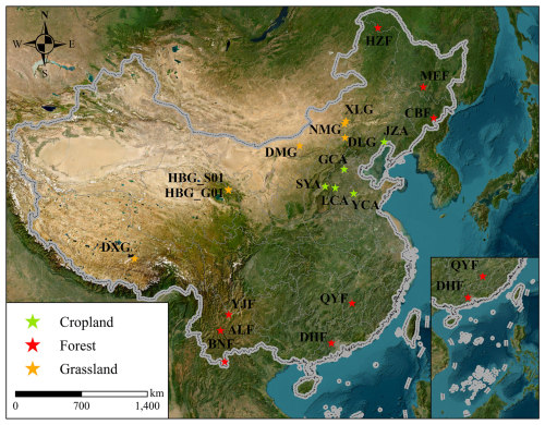
Figure 1 The location map of the flux site is based on the map approved by the National Surveying and Mapping Bureau of China (approval no. GS (2019)1822). The topographic map is derived from data provided by Esri, Maxar, Earthstar Geographics, and the GIS User Community (Service Layer Credits).

Table 1 Basic information on the 20 flux stations.

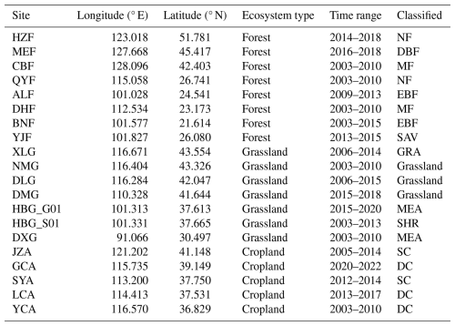
Note that vegetation types in the table are classified based on the land cover characteristics of each flux site and are used in subsequent model simulations. NF: needle-leaved forest; DBF: deciduous broadleaf forest; MF: mixed forest; EBF: evergreen broadleaf forest; SAV: savannas; GRA: typical grassland; MEA: alpine meadow; SHR: shrubs; SC: single cropping; DC: double cropping.

2.2 Data

2.2.1 Eddy covariance data

EC data were collected at 20 sites, including 8 forests sites, 7 grasslands sites, and 5 cropland sites (Table 1). Flux and meteorological data were collected every half hour from the mentioned sites. The flux and meteorological data underwent standardized quality control and corrections, ensuring high reliability and making them suitable for validating various GPP models and remote sensing observations. However, ER data were missing at some sites (DLG, LCA, XLG). To address this, the Lloyd & Taylor equation (Reichstein et al., 2005; Lloyd and Taylor, 1994) was applied to estimate ER based on nocturnal respiration data. Daytime and nighttime periods were distinguished using shortwave radiation (Rg), with a threshold of 10 W m⁻². The temperature–response relationship derived from nighttime ER was extrapolated to estimate daytime ER. This is a commonly used method for processing flux data at flux tower sites.

$$\begin{array}{}\text{(1)}& {\displaystyle }{R}_{\text{eco}}=R_{\text{eco.ref}}\exp \left(E_{\mathrm{0}}\left({\displaystyle \frac{\mathrm{1}}{T_{\text{ref}}-T_{\mathrm{0}}}}-{\displaystyle \frac{\mathrm{1}}{T_{\text{air}}-T_{\mathrm{0}}}}\right)\right)\text{(2)}& {\displaystyle }\text{GPP}=\text{ER}-\text{NEE}\end{array}$$

In Eq. (1), R_eco is the nocturnal ecosystem respiration value; R_eco.ref is the ER value at the reference temperature; T_ref is the reference temperature (298.16 K); E₀ is constant (308.56 K); T₀ is the minimum temperature at which respiration stops, set at 227.13 K; and T_air is the air temperature or soil temperature (K). Daytime GPP was then estimated by subtracting NEE from the total daytime ER.

2.2.2 MODIS data

In this study, remote sensing data were primarily obtained from the Moderate Resolution Imaging Spectroradiometer (MODIS). MODIS data offer a spatial resolution of 500 m and an 8 d temporal resolution. These datasets were sourced from the Google Earth Engine (GEE) platform (Gorelick et al., 2017). To align with the spatial and temporal scales of flux tower observations and reduce the impact of missing data (Schmid, 2002), we applied the Savitzky–Golay smoothing filter with a window size of 10 to process the vegetation indices. Vegetation and water indices derived from MODIS data included the enhanced vegetation index (EVI), normalized difference vegetation index (NDVI), and land surface water index (LSWI), which were calculated using the formulas presented in Table 2.

Table 2 Predictor variables for driving the FLAML models and their specifications.

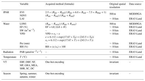
EVI: enhanced vegetation index, NDVI: normalized difference vegetation index, LAI: leaf area index, LSWI: land surface water index, EF: evaporative fraction, SW: surface soil moisture, VPD: vapor pressure deficit, Pre: precipitation, RH: relative humidity, PAR: photosynthetically active radiation, and T: air temperature. NF: needle-leaved forest; DBF: deciduous broadleaf forest; MF: mixed forest; EBF: evergreen broadleaf forest; SAV: savannas; GRA: typical grassland; MEA: alpine meadow; SHR: shrubs; SC: single cropping; DC: double cropping. In the formulas for EVI and NDVI, R_nir, R_red, R_blue, and R_swir represent the surface reflectance in the near-infrared (NIR), red, and blue spectral bands, respectively. In the EF calculation formula, LE refers to latent heat flux, while H represents sensible heat flux. In the RH formula, e is the actual vapor pressure, e_s is the saturation vapor pressure, T_d is the dew point temperature, and T is the air temperature.

2.2.3 ERA5-Land

ERA5-Land (Hersbach et al., 2020) is a global high-resolution reanalysis dataset produced by the European Centre for Medium-Range Weather Forecasts (ECMWF) under the Copernicus Climate Change Service (C3S). It provides hourly land surface variables at a spatial resolution of 0.1°, generated using a dedicated land surface model driven by the ERA5 climate reanalysis. The dataset integrates advanced land surface modeling and data assimilation techniques, offering a wide range of variables such as air temperature, soil moisture, precipitation, and snow depth. In this study, site-specific variables including air temperature (T), soil water content (SW), precipitation (Pre), and leaf area index (LAI) were extracted from ERA5-Land. In addition, photosynthetically active radiation (PAR), evapotranspiration fraction (EF), VPD, and relative humidity (RH) were calculated and derived from available ERA5-Land variables using GEE.

2.2.4 SPEI Database, Version 2.10

The SPEI Database, Version 2.10 (Vicente-Serrano et al., 2010), provides global data of the Standardized Precipitation-Evapotranspiration Index (SPEI) across temporal scales from 1 to 48 months. Developed by the Climatic Research Unit (CRU), this dataset combines precipitation and potential evapotranspiration (PET) to assess drought conditions. Negative SPEI values indicate drought, while positive values signify wet periods. In this study, SPEI values less than −1.5 were used to identify drought months at each flux station, highlighting significant moisture deficits that affect vegetation growth and ecosystem productivity (Qian et al., 2024).

2.3 Model construction

Most LUE models typically incorporate four main groups of variables: PAR, fPAR, temperature, and water-related stress indicators. In previous studies, vegetation indices such as EVI, NDVI, or LAI have been widely used as proxies for fPAR, representing the fraction of PAR absorbed by the plant canopy (Chang et al., 2023; Qian et al., 2024). In this study, we selected six water-related indicators based on their ecological relevance: plant-based indicators (LSWI and EF), soil-based indicators (SW), and atmospheric indicators (VPD, precipitation, and relative humidity). Previous research has shown that plant-based indicators like LSWI and EF effectively capture canopy-level drought stress (Anderson et al., 2007; Xiao et al., 2004). Soil moisture regulates water availability at the root level, which strongly influences photosynthetic activity, particularly under water-limited conditions (Vicca et al., 2014; Reichstein et al., 2007). Meanwhile, atmospheric indicators such as VPD, precipitation, and RH influence stomatal conductance and transpiration by altering the vapor pressure gradient between the leaf surface and the surrounding air (Wang et al., 2018; Novick et al., 2016). To assess the relative importance of these different types of water stress indicators in estimating GPP, we developed machine learning models using each group individually. This allowed us to identify the most effective type of water-related variable for simulating GPP across diverse ecosystems within the LUE modeling framework.

The flowchart of this study is shown in Fig. 2.

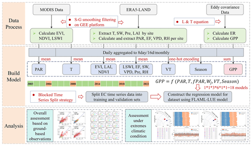
Figure 2 Flowchart of this study. S-G smoothing filtering: Savitzky–Golay smoothing filtering method, L & T equation: Lloyd & Taylor equation.

2.3.1 Data pre-processing and splitting strategy

The primary datasets for estimating GPP with FLAML-LUE models include multi-year continuous EC flux data, satellite-based observations, and ERA5-Land climate reanalysis data. Prior research (Jung et al., 2011) has demonstrated notable seasonal fluctuations in GPP; we divided the time series data into four distinct seasons. Moreover, the vegetation cover type, which varies across different ecosystems, greatly impacts the accuracy of GPP simulation (Chang et al., 2023). Hence, we integrate vegetation type as a factor in our model.

The pre-processed dataset was divided into training and testing sets using the Blocked Time Series Split strategy. Given the temporal dependency of the data, standard cross-validation is not suitable for time series analysis (Reichstein et al., 2019). Instead, a block-based and non-continuous split is applied to preserve the temporal structure. In this approach, the time series is partitioned into several non-overlapping continuous training blocks (e.g., 2003–2005, 2007–2009, 2011–2013, 2015–2017, 2019–2021), with independent years reserved as the validation set following each training block (e.g., 2006, 2010, 2014, 2018, 2022). This strategy ensures that the temporal order is maintained, preventing future data from leaking into the training process and thus avoiding invalid predictions. Additionally, the method incorporates validation over multiple periods, enabling the assessment of model generalization across different climate conditions, which is crucial for evaluating the model's robustness under varying environmental scenarios.

2.3.2 Automated machine learning (AutoML)

Instead of applying a specific ML method like RF for building regression models, we utilize the lightweight Python library “FLAML” version 2.3.3 (Wang et al., 2021a) for the AutoML task (Metin and Bilgin, 2024). FLAML optimizes the search process by balancing computational cost and model error, iteratively selecting the learner, hyperparameters, sample size, and resampling strategy (Wang et al., 2021a).

For our regression tasks, AutoML was configured with the “auto” option for the estimator list, focusing on optimizing the R² metric and using a time budget of 120 s per run. Under this “auto” setting, FLAML explores a variety of built-in regression estimators, including the following:

1. LightGBM (Ke et al., 2017), a histogram-based gradient boosting method designed for speed and scalability;

2. XGBoost (Chen and Guestrin, 2016), a regularized gradient boosting framework known for its robustness and accuracy;

3. CatBoost (Prokhorenkova et al., 2018), which efficiently handles categorical features and reduces overfitting via ordered boosting;

4. Random Forest (Breiman, 2001), an ensemble method utilizing bootstrap aggregation of decision trees;

5. Extra Trees (Geurts et al., 2006), which enhances randomness in split point selection for tree construction;

6. Histogram-based Gradient Boosting (Brownlee, 2020), which accelerates training through feature binning;

7. K-nearest neighbors (Cover and Hart, 1967), a non-parametric distance-based algorithm relying on local data density;

8. Transformer models (Vaswani et al., 2023), deep learning architectures leveraging self-attention mechanisms, adapted here for structured data regression.

Collectively, these estimators span a broad algorithmic spectrum, including ensemble learning, distance-based methods, and neural networks, enabling FLAML to automatically identify the optimal model architecture for the dataset and objective.

2.3.3 Model development

Eighteen FLAML-LUE model variations were constructed for all sites by combining different permutations of six input factor groups, as described in Eq. (3) and detailed in Table 3. Technically, the term “FLAML-LUE” does not refer to a direct implementation of a mechanistic LUE model. Instead, it reflects a hybrid modeling strategy, through which we incorporate key explanatory variables that originate from LUE theory – such as fPAR, light-use efficiency modifiers, and environmental stress indicators (e.g., VPD, temperature, and water stress indices) – into an automated machine learning framework (FLAML). These variables capture the main drivers of vegetation productivity in traditional LUE models. Their integration enables FLAML to build models that are both ecologically grounded and predictive, effectively balancing model interpretability and accuracy.

$$\begin{array}{}\text{(3)}& \text{GPP}=f(\text{PAR},T,\text{fPAR},W_j,\text{VT},\text{season}),\end{array}$$

where fPAR includes EVI, NDVI, and LAI; W_j denotes moisture factors including LSWI, EF, SW, PDSI, Pre, and RH; VT represents vegetation types, in which forest ecosystems include EBF, DBF, NF, MF, and SAV, grassland ecosystems include GRA, MEA, and SHR, and farmland ecosystems include SC and DC; and season represents the season in which the original data were acquired.

Table 3 Input variable combinations of fPAR and water stress indicators.

EVI: enhanced vegetation index, NDVI: normalized difference vegetation index, LAI: leaf area index, LSWI: land surface water index, EF: evaporative fraction, SW: surface soil moisture, VPD: vapor pressure deficit, Pre: precipitation, RH: relative humidity.

2.3.4 Model performance evaluation methods

To evaluate the simulation accuracy of the FLAML-LUE model in estimating GPP, we employed a suite of widely used statistical metrics to quantify the agreement between modeled and observed values (Qian et al., 2024; Chang et al., 2023; Tramontana et al., 2016). Specifically, we calculated the coefficient of determination (R²), Pearson correlation coefficient (R), normalized unbiased root mean square error (nuRMSE), and normalized standard deviation (NSD; ${\widehat{\mathit{\sigma }}}_{\mathrm{f}}$), based on GPP observations from flux towers and model simulations. The Taylor diagram (Taylor, 2001) was utilized to provide a visual summary of the model's performance, incorporating R, nuRMSE, and NSD.

$$\begin{array}{}\text{(4)}& {\displaystyle }{R}^{\mathrm{2}}={\displaystyle \frac{{\left[{\sum }_{t=\mathrm{1}}^T(f_t-\stackrel{\mathrm{‾}}{f})(o_t-\stackrel{\mathrm{‾}}{o})\right]}^{\mathrm{2}}}{{\sum }_{t=\mathrm{1}}^T(f_t-\stackrel{\mathrm{‾}}{f}{)}^{\mathrm{2}}{\sum }_{t=\mathrm{1}}^T(o_t-\stackrel{\mathrm{‾}}{o}{)}^{\mathrm{2}}}}\text{(5)}& {\displaystyle }R={\displaystyle \frac{\frac{\mathrm{1}}{T}{\sum }_{t=\mathrm{1}}^T(f_t-\stackrel{\mathrm{‾}}{f})(o_t-\stackrel{\mathrm{‾}}{o})}{{\mathit{\sigma }}_{\mathrm{f}}{\mathit{\sigma }}_{\mathrm{o}}}}\text{(6)}& {\displaystyle }\begin{array}{rl}\text{nuRMSE}& ={\displaystyle \frac{\text{uRMSE}}{{\mathit{\sigma }}_{\mathrm{o}}}}\\ & ={\displaystyle \frac{\mathrm{1}}{{\mathit{\sigma }}_{\mathrm{o}}}}\sqrt{{\displaystyle \frac{\mathrm{1}}{T}}{\sum }_{t=\mathrm{1}}^T{\left[(f_t-\stackrel{\mathrm{‾}}{f})-(o_t-\stackrel{\mathrm{‾}}{o})\right]}^{\mathrm{2}}}\end{array}\text{(7)}& {\displaystyle }{\widehat{\mathit{\sigma }}}_{\mathrm{f}}={\displaystyle \frac{{\mathit{\sigma }}_{\mathrm{f}}}{{\mathit{\sigma }}_{\mathrm{o}}}}={\displaystyle \frac{\mathrm{1}}{{\mathit{\sigma }}_{\mathrm{o}}}}\sqrt{{\displaystyle \frac{\mathrm{1}}{T}}{\sum }_{t=\mathrm{1}}^T{\left((f_t-\stackrel{\mathrm{‾}}{f})\right)}^{\mathrm{2}}}\text{(8)}& {\displaystyle }{\mathit{\sigma }}_{\mathrm{o}}=\sqrt{{\displaystyle \frac{\mathrm{1}}{T}}{\sum }_{t=\mathrm{1}}^T{\left((o_t-\stackrel{\mathrm{‾}}{o})\right)}^{\mathrm{2}}},\end{array}$$

where o_t represents the observed GPP from the flux tower, f_t denotes the simulated GPP from FLAML-LUE model, $\stackrel{\mathrm{‾}}{o}$ represents the average of observed GPP from the flux tower, $\stackrel{\mathrm{‾}}{f}$ represents the average of estimated GPP from the GPP product, t represents the corresponding ID for the GPP data, and n represents the total count of GPP data for the site. σ_o represents the standard deviations of the observed GPP. A higher R² value indicates better consistency between the estimated GPP and the flux GPP.

In addition, the Taylor skill score (TSS) was computed to quantitatively assess the overall agreement between simulations and observations, with higher values indicating better performance.

$$\begin{array}{}\text{(9)}& \text{TSS}={\displaystyle \frac{\mathrm{4}(\mathrm{1}+R)}{({\widehat{\mathit{\sigma }}}_{\mathrm{f}}+\frac{\mathrm{1}}{{\widehat{\mathit{\sigma }}}_{\mathrm{f}}}{)}^{\mathrm{2}}(\mathrm{1}+R_{\mathrm{0}})}},\end{array}$$

where σ_f represents the standard deviations of the model simulation, and R₀ denotes the maximum possible correlation coefficient (in this study, R₀=1). The TSS ranges from 0 to 1, with a higher TSS indicating better overall model performance relative to the observations.

To further investigate model bias across sites, the percent bias (PBias) was introduced (Qian et al., 2024). Positive PBias values indicate overestimation by the model, while negative values suggest underestimation. The closer the PBias is to zero, the more accurate the model's estimations. The calculation formula is as follows:

$$\begin{array}{}\text{(10)}& \text{PBias}={\displaystyle \frac{{\sum }_{t=\mathrm{1}}^T(f_t-o_t)}{{\sum }_{t=\mathrm{1}}^T{o}_t}}\times \mathrm{100}\mathit{\%}.\end{array}$$

To evaluate the model's ability to capture GPP dynamics under extreme climate conditions, we identified heat waves and high-VPD events using the 95th percentile of historical meteorological records (Stefanon et al., 2012; Anderson and Bell, 2010). Drought events were defined as months with SPEI less than −1.5 (Ayantobo et al., 2019; Gumus, 2023). These definitions enabled us to evaluate model performance under extreme environmental stresses (Qian et al., 2024, 2023).

$$\begin{array}{}\text{(11)}& {\text{CV}}_{\text{RMSE}}={\displaystyle \frac{\sqrt{\frac{\mathrm{1}}{T}{\sum }_{t=\mathrm{1}}^T(f_t-o_t{)}^{\mathrm{2}}}}{\stackrel{\mathrm{‾}}{o}}}\times \mathrm{100}\mathit{\%}\end{array}$$

To determine whether model performance differed significantly across temporal resolutions (daily, 8 d, 16 d, and monthly), we conducted paired t tests at a 0.05 significance level. All statistical analyses were performed in Python 3.9 using libraries including numpy, pandas, scipy, matplotlib, sklearn, and flaml. Complementary visualizations were produced in R using ggplot2, ggpubr, and readxl.

3 Results

3.1 Overall model evaluation based on ground-based observations

To evaluate the model performance at the site level, the accuracy of the 18 FLAML-LUE models was assessed using test datasets from individual flux tower sites. The algorithms selected by each FLAML-LUE model are listed in Table S1 in the Supplement. Notably, the Extra Trees algorithm was most frequently chosen as the best-performing model. Extra Trees is an ensemble method that constructs multiple unpruned decision trees and introduces high randomness in both feature and threshold selection, which enhances generalization and reduces overfitting, particularly in noisy or high-dimensional datasets. The consistent selection of Extra Trees suggests that FLAML tends to favor models with higher stochasticity and ensemble structures under the given data and computational constraints.

Figure 3 presents the R, nuRMSE, and NSD values for the 18 models. As shown in Fig. 3u, the model performance shows relatively small differences across different combinations of input indicators. Specifically (Table 4), the overall R² of the different FLAML-LUE models ranged from 0.78 to 0.82, while nuRMSE values ranged from 0.4240 to 0.4670.

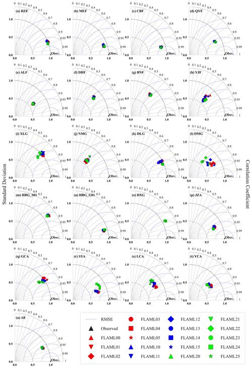
Figure 3 Normalized Taylor diagrams showing the performance of the FLAML-LUE model at various sites based on observed GPP data. Each point represents a specific combination of fPAR and water stress factor used in the model simulation. Different colors denote different fPAR products: red for EVI, blue for NDVI, and green for LAI. Marker shapes indicate the type of water stress factor: “+” for LSWI, “×” for EF, diamond for SW, circle for VPD, square for Pre, and star for RH. Points closer to the reference point (R=1, NSD=1) indicate better agreement between simulated and observed GPP. Panels (a)–(h) correspond to eight forest sites, (i)–(o) to seven grassland sites, and (p)–(t) to five cropland sites. Panel (u) presents an overall model evaluation on the validation dataset across all sites.

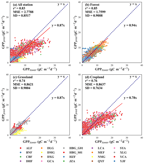
Figure 4 Scatter plot of observed GPP vs. simulated GPP. Different colored dots represent different sites. Note that the simulated GPP values represent the mean of FLAML00 to FLAML25.

Among the fPAR-related indices, the model driven by EVI performed slightly better (R²=0.82, nuRMSE=0.4265) than models driven by NDVI (R²=0.80, nuRMSE=0.4524) and LAI (R²=0.79, nuRMSE=0.4561). Regarding moisture stress indicators, the model using LSWI as input achieved the best performance (R²=0.82, nuRMSE=0.4298), followed by models using VPD (R²=0.80, nuRMSE=0.4455) and RH (R²=0.80, nuRMSE=0.4450). Models driven by EF (R²=0.80, nuRMSE=0.4487), SW (R²=0.80, nuRMSE=0.4505), and Pre (R²=0.80, nuRMSE=0.4503) performed slightly worse, though the differences were minimal.

Table 4 Summary of evaluation metrics for FLAML-LUE model performance across all validation sites.

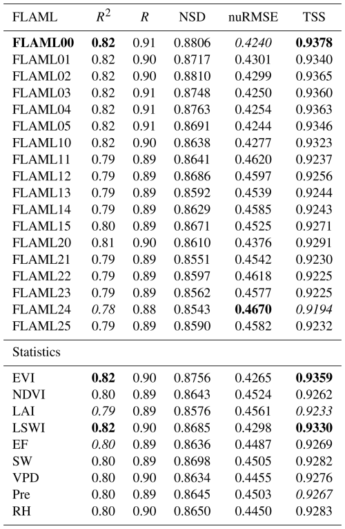
Note that the statistics represent the mean values of R², R, NSD, nuRMSE, and TSS across all combinations in which the respective variable was involved. Bold numbers indicate the highest values, while italic numbers represent the lowest values.

As shown in Table 5, the performance of the FLAML-LUE model varies considerably across different sites, with the average R² ranging from 0.17 at DXG to 0.92 at CBF and HBG_G01. Notably, this variation was primarily attributed to site-level differences rather than the combinations of input indicators (Fig. 3), highlighting the influence of land cover type and climatic conditions on model performance.

Table 5 Mean evaluation metrics for different combinations of fPAR and water stress indicators at each site. Bold numbers indicate the highest values, while italic numbers represent the lowest values.

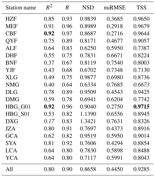
The best model performance was observed at the HZF, MEF, CBF, and HBG_G01 sites (R²>0.85, TSS>0.9), followed by QYF, DLG, JZA, and SYA (R²>0.75, TSS>0.88). Within forest ecosystems, the model performed better in MF, NF, and DBF than in EBF (ALF, BNF) and savannas (YJF). MF, which includes both evergreen conifers and deciduous broadleaf species, exhibits distinct seasonal variations that can be effectively captured by satellite imagery. In contrast, EBF shows minimal seasonal greenness variation, leading to larger modeling bias in GPP estimation.

In grassland ecosystems, the model performed better for shrublands and typical steppe than for alpine meadows (Tables S4 and S5). Alpine meadows, characterized by short growing seasons and harsh high-altitude climates, often experience strong environmental disturbances and large GPP fluctuations, making them more difficult to model accurately. In contrast, typical steppe and alpine shrublands display clearer phenological rhythms and stronger photosynthetic activity, making their GPP dynamics easier to capture.

In cropland ecosystems, all sites demonstrated relatively strong model performance (R²>0.6, TSS>0.80). Compared to natural grasslands or alpine meadows, croplands are usually monocultures with stable phenology and simpler canopy structures, which aid in more accurate GPP modeling.

Notably, at the DXG site, the model achieved a high TSS (0.8326) but a relatively low R² (0.17), primarily due to the large performance variation among different index combinations. As shown in Table S4, all six NDVI-driven models (FLAML10-FLMAL15) have negative R² values, significantly reducing the overall model accuracy at this site.

From an ecosystem perspective, Fig. 4 and Table 7 indicates that the FLAML-LUE model achieves the highest fitting accuracy in forest ecosystems (R²=0.83, nuRMSE=0.4162), followed by cropland ecosystems (R²=0.72, nuRMSE=0.5258) and the lowest in grassland ecosystems (R²=0.71, nuRMSE=0.5407). The slope of the fitted line in Fig. 7 is less than 1 for all ecosystem types, indicating that the FLAML-LUE model tends to underestimate GPP, particularly in croplands and grasslands.

Tables S2 and S3 and Table 6 collectively demonstrate that the model's performance varies across ecosystem types depending on the choice of fPAR-related variables. In forest ecosystems, the model is relatively insensitive to different fPAR and water-related inputs, with the LAI-driven model achieving the best performance. This can be attributed to LAI's ability to capture forest canopy structure, thereby improving fPAR estimates. In contrast, the model's performance is more sensitive to the choice of input variables in cropland and grassland ecosystems. In croplands, the EVI-driven model performs best, followed by LAI and then NDVI, although the performance differences are moderate. In grasslands, however, the NDVI-driven model performs worst, especially at the DXG site, likely due to NDVI's sensitivity to soil background and saturation in sparse and heterogeneous vegetation. EVI, with reduced saturation and higher sensitivity to biomass, shows better performance in structured cropland areas. Overall, the EVI- and LSWI-driven model (FLAML00) exhibits the best performance across all ecosystem types.

Table 6 Summary of evaluation metrics for FLAML-LUE model performance across all validation sites. Bold numbers indicate the highest values, while italic numbers represent the lowest values.

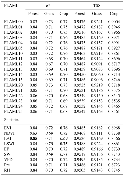
Table 7 Mean evaluation metrics for different combinations of fPAR and water stress indicators across various ecosystems.

Note that the evaluation metrics for all sites and different ecosystem types were calculated based on the average of 18 simulation results.

To further investigate model accuracy across different land cover types, Fig. 5 presents the R² values of five forest types, three grassland types, and two cropland types under different models. In general, model performance varies little within the same land cover type but differs substantially across types. Specifically, DBF, NF, MF, and SC exhibit higher simulation accuracy, followed by GRA, SHR, and DC, while EBF, SAV, and MEA perform the worst. These results are consistent with the Taylor diagram in Fig. 3.

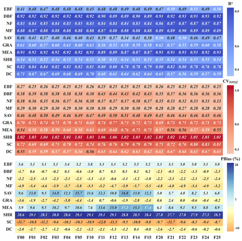
Figure 5 Comparison of R², CV_RMSE, and PBias of GPP estimates from different FLAML-LUE models across various land cover types. Note that F00 represents FLAML00 and so on.

Regarding CV_RMSE, SHR shows the largest error, followed by MEA, GRA, SC, and DC, while the five forest types show the smallest errors. This may be attributed to the greater GPP variability in grassland and cropland ecosystems, which are more strongly influenced by climatic variability and anthropogenic activities, leading to higher model uncertainty. In contrast, forest ecosystems have more stable structures and continuous carbon exchange processes, resulting in more robust model performance. Although alpine meadow is classified as grassland ecosystems, their extreme climatic conditions, short growing season, and high sensitivity to temperature and precipitation further increase the uncertainty of GPP simulation, leading to higher errors.

In terms of PBias, SHR consistently shows a pronounced overestimation across all models. Similarly, SAV and MEA are also generally overestimated in all models, though to a lesser extent than SHR. EBF exhibits a slight overestimation as well. Other vegetation types display only minor underestimation or overestimation. Overall, the models perform best for DBF, NF, and MF, followed by EBF, MEA, SC, and DC, while the simulation accuracy is relatively poor for SAV, SC, and especially SHR.

Biases also differ among grassland ecosystems, especially for typical grasslands, alpine meadows, and shrublands. Typical grasslands tend to be underestimated, while alpine meadows and shrublands are often overestimated. These biases may result from the model's limited ability to capture seasonal changes in water availability and its interaction with temperature. Typical grasslands usually show high productivity when water is sufficient, especially in spring and summer. If the model fails to reflect these seasonal patterns, it can lead to underestimation. In contrast, productivity in alpine meadows is mainly limited by low temperatures and a short growing season. If the model does not fully consider these constraints, it may overestimate photosynthesis and thus GPP. For shrublands, overestimation may be due to high spatial heterogeneity, including a mix of shrubs, grasses, and bare soil. This complexity is difficult to capture in remote sensing data (e.g., fPAR) and model inputs, leading to possible overestimation of productivity.

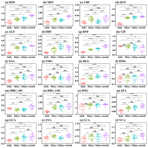
Figure 6 Asterisks indicate significant differences between the R² at the four temporal resolutions (Kruskal–Wallis test): ${}^{\ast \ast \ast \ast }$ p values<0.0001, ${}^{\ast \ast \ast }$ p values<0.001, ${}^{\ast \ast }$ p values<0.01, and ^∗ p values≤0.05. ns indicates no significance (p>0.05).

Across the four temporal scales, the performance of the 18 FLAML-LUE models improves as the temporal resolution becomes coarser. The average R² across 20 sites increases from 0.64 at the daily scale to 0.74 at the monthly scale (Table S8), while the average nuRMSE decreases from 0.5518 to 0.4088. Paired t tests show that, except for YJF, NMG, DMG, DXG, and YCA, the FLAML-LUE model exhibits significantly lower R² at the daily scale than at longer temporal scales (p<0.05, Fig. 6). For these five sites, model performance remains relatively stable across different temporal scales.

Furthermore, compared to the daily scale, the nuRMSE decreases by 12.97 %, 16.52 %, and 25.92 % at the 8 d, 16 d, and monthly scales, respectively, indicating that the uncertainty of the FLAML-LUE model is significantly reduced at coarser temporal resolutions.

Overall, the accuracy of FLAML-LUE models constructed using different combinations of fPAR and water stress indicators showed limited variation, with the FLAML00 model (fPAR = EVI, water = LSWI) demonstrating the best performance. However, the model exhibited considerable differences in performance across ecosystem types, with the highest accuracy observed in forest ecosystems, followed by croplands and then grasslands. Further analysis by specific vegetation cover types revealed that the model performed best for DBF, NF, and MF, followed by GRA, MEA SC, and DC, while its performance was relatively poor for EBF, SAV, and particularly SHR (PBias>27 %, CV_RMSE>1, R²<0.6). In addition, evaluation across different temporal scales indicated that model uncertainty decreased with increasing time intervals, suggesting that the FLAML-LUE model exhibits greater robustness and reliability at coarser temporal resolutions.

3.2 Model evaluation under extreme climatic conditions

Numerous studies have demonstrated that climate extremes such as heat waves, droughts, and high atmospheric VPD can substantially alter ecosystem dynamics and reduce carbon uptake capacity (Frank et al., 2015; Reichstein et al., 2013). These extreme events can suppress photosynthesis, increase respiration, and disrupt the balance of carbon exchange between vegetation and the atmosphere. In order to evaluate the robustness and reliability of the FLAML-LUE models under such stress conditions, this study further investigates model performance in simulating GPP under three types of climate extremes: high temperature, high VPD, and drought. By analyzing the response of model accuracy and bias under these scenarios, we aim to assess its applicability and limitations in extreme environmental conditions.

3.2.1 Performance under high-temperature events

Figure 7 shows the performance of 18 FLAML-LUE models under high-temperature and non-high-temperature conditions. The results indicate a significant decline in model accuracy under high-temperature conditions. As shown in Fig. 7a, the models perform well under non-high-temperature conditions, with the R values of all 18 FLAML-LUE models exceeding 0.9. However, under high-temperature conditions, the Taylor diagram reveals a significant decrease in model performance, with correlation coefficients dropping and a substantial increase in nuRMSE, indicating a reduced ability to capture GPP dynamics.

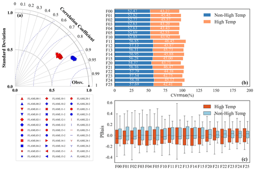
Figure 7 The comparison of GPP products performance under high temperature and non-high temperature (in the Taylor diagram, 1 represents high temperature, and 2 represents non-high temperature).

Interestingly, as shown in Fig. 7b, the CV_RMSE values under non-high-temperature conditions are generally higher than under high-temperature conditions. This may be due to higher observed GPP values under high temperatures, resulting in a larger denominator for CV_RMSE, which can reduce the CV_RMSE despite larger prediction errors. Overall, the difference in prediction bias between high-temperature and non-high-temperature conditions is minimal.

Figure 7c shows that, under high-temperature conditions, the PBias fluctuates more significantly, with more stations showing severe overestimation or underestimation. Specifically, some models (e.g., FLAML00, FLAML01, FLAML11, FLAML15, FLAML21) overestimate GPP at certain sites under high-temperature conditions, while all models show more severe underestimation at other sites. Models driven by LAI (FLAML20 – FLAML25) exhibit smaller bias variations under non-high-temperature conditions, with PBias mainly ranging from −0.3 to 0.3.

In conclusion, high-temperature conditions increase model uncertainty, with all models exhibiting varying degrees of overestimation or underestimation across sites. Models incorporating VPD, precipitation, and relative humidity as water stress factors perform better overall, indicating greater robustness under high-temperature stress.

Differences in model performance under high-temperature and non-high-temperature conditions are pronounced across various land cover types. Figure 8 compares the estimation accuracy of different land cover types under both conditions. Overall, model accuracy in simulating GPP is significantly lower under high-temperature conditions, with R² values showing a notable decline. Specifically, for the NF type, the R² under high temperatures approaches a negative value, indicating very low explanatory power, whereas under non-high-temperature conditions, R² ranges from 0.83 to 0.87. Notably, the FLAML13 model for savannas shows a drastic decrease in R² from 0.38 under non-high-temperature conditions to −1.46 under high-temperature conditions, performing even worse than the mean of the data during high temperatures.

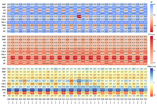
Figure 8 Comparison of statistical indicators (R², CV_RMSE, PBias) of the FLAML-LUE model under high-temperature conditions and non-high-temperature conditions for different land cover types (1 represents high temperature, and 2 represents non-high temperature).

Corresponding to Fig. 7, CV_RMSE is generally lower under high-temperature conditions than under non-high-temperature conditions. The SHR type exhibits a higher coefficient of variation, while PBias shows more pronounced fluctuations. For SHR and EBF, the models tend to overestimate GPP under both temperature conditions, with overestimation more pronounced under high temperatures. In contrast, MEA shows underestimation under high-temperature conditions but overestimation under non-high-temperature conditions. Overall, most land cover types exhibit a greater degree of underestimation under high-temperature conditions. Nevertheless, the MF type maintains relatively high simulation accuracy. In contrast, the DBF, NF, and SC types are more strongly affected by high temperatures, with NF showing negative simulation accuracy under high-temperature conditions and SC exhibiting marked variations in PBias.

3.2.2 Performance under high VPD

Figure 9 shows the performance of the 18 FLAML-LUE models under high- and non-high-VPD conditions. Unlike the high-temperature scenario, the statistical metrics of all models exhibit only a slight decline under high VPD, indicating a less pronounced impact on model performance. As shown in Fig. 9a, the variability in model performance increases under high-VPD conditions. However, Fig. 9b reveals that CV_RMSE values are generally higher under non-high-VPD conditions, a trend consistent with the results observed under high-temperature conditions.

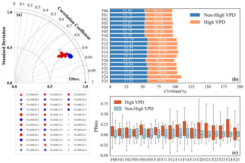
Figure 9 The comparison of GPP products performance under high VPD and non-high VPD (in the Taylor diagram, 1 represents high VPD, and 2 represents non-high VPD).

Under high VPD, PBias exhibits significant fluctuations compared to non-high-VPD conditions (Fig. 9c). Specifically, the average PBias across sites is higher under high VPD, whereas it is lower under non-high VPD. In high-VPD conditions, models driven by EVI show smaller differences in PBias across sites, with values primarily ranging from −0.4 to 0.5. In contrast, FLAML05 shows larger differences in PBias between sites under non-high VPD, with overestimations at some sites. Overall, model performance under high VPD shows greater uncertainty, with both overestimations and underestimations occurring across different sites. In general, EVI-driven models perform more consistently under both high- and non-high-VPD conditions.

Model performance also differs across land cover types under high- and non-high-VPD conditions. Figure 10 compares the estimation accuracy for various land cover types under both conditions. Overall, GPP simulation accuracy for certain cover types (e.g., DBF, MF, MEA, SC, DC) shows little difference between high- and non-high-VPD conditions. Although R² values for some land cover types are significantly lower under high VPD than under non-high VPD, the impact of high VPD on model performance is smaller compared to high temperature. The most notable example is the FLAML13 model for savannas, where R² drops significantly from −1.46 under non-high VPD to −0.39 under high VPD, performing worse than the mean data value under high VPD.

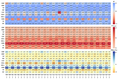
Figure 10 Comparison of statistical indicators (R², CV_RMSE, PBias) of the FLAML-LUE model under high-VPD conditions and non-high-VPD conditions for different land cover types (1 represents high VPD, and 2 represents non-high VPD).

Similar to high-temperature conditions, CV_RMSE under high VPD is generally lower than under non-high VPD. MEA shows a larger coefficient of variation, and PBias exhibits more noticeable fluctuations. For the EBF and SHR type, models tend to overestimate GPP in both high- and non-high-VPD conditions, with the overestimation being more pronounced under high VPD. SC and GRA models show significant underestimation under high VPD. DBF, NF, and MF perform relatively well under high VPD, while SC underestimates GPP under both conditions, and DC overestimates GPP under high VPD but underestimates it under non-high VPD. Overall, compared to high-temperature conditions, the effect of high VPD on estimation errors is smaller across different land cover types.

3.2.3 Performance under drought conditions

Figure 11 presents the simulation performance of the 18 FLAML-LUE models under drought and non-drought conditions. Unlike the decline in performance under high-temperature and high-VPD conditions, the model shows similar or even slightly better accuracy under drought compared to non-drought conditions. This may be attributed to an overall reduction in GPP and its variability during drought periods, which potentially makes it easier for the models to capture the general trend and thereby improves simulation accuracy.

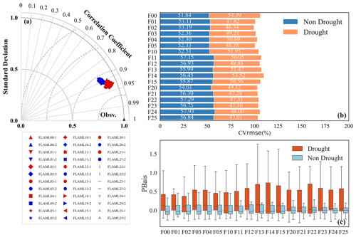
Figure 11 The comparison of GPP products performance under drought and non-drought (in the Taylor diagram, 1 represents drought, and 2 represents non drought).

Compared to the box plots under non-drought conditions, drought notably increases the variability in PBias across sites for all models, particularly due to substantial overestimation at certain sites. In contrast, the degree of underestimation remains similar to that under non-drought conditions. Among the models, those driven by EVI exhibit the best overall performance, followed by those using LAI as the vegetation indicator.

Figure 12 shows that drought substantially affects GPP estimation accuracy across most land cover types. For certain types, such as savannas and deciduous broadleaf forests, no data were available during drought months, making performance evaluation under drought impossible. For other land cover types, the impact of drought varies significantly. Specifically, EBF, MEA, and DC show higher R² values under drought, while NF, MF, GRA, SHR, and SC perform better under non-drought conditions. Among them, MF and SHR have the lowest simulation accuracy under drought but perform relatively well during non-drought periods.

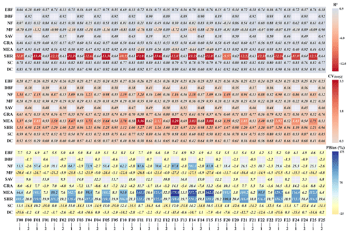
Figure 12 Comparison of statistical indicators (R², CV_RMSE, PBias) of the FLAML-LUE model under drought conditions and non-drought conditions for different land cover types (1 represents drought, and 2 represents non-drought).

Regarding CV_RMSE, all land cover types except MEA and NF exhibit lower values under drought conditions, consistent with the results in Fig. 11a. MEA shows the largest coefficient of variation, indicating greater variability in model performance under drought. In terms of PBias, NF, MEA, and SHR exhibit the highest errors. On average, model errors increase under drought across most land cover types. Except for EBF and GRA, most types show severe overestimation or underestimation during drought periods.

4 Discussion

Model performance is highly influenced by the algorithms used, the underlying processes, and how GPP responds to varying environmental conditions (Chang et al., 2023). A detailed comparison of the FLAML-LUE models across different ecosystems showed that performance varied depending on the input variables, vegetation types, and timescales (Chang et al., 2023; Harris et al., 2021).

4.1 Performance comparison of FLAML-LUE models for different ecosystems

In this study, FLAML-LUE models were constructed for different combinations of variables and different timescales based on AutoML algorithms. On the whole, the modeled GPP values agree well with the GPP estimated based on the EC tower, and the FLAML-LUE models performed better in capturing the magnitude and seasonal dynamics of the GPP, which indicated that it was feasible to estimate the GPP using AutoML algorithms. Further, all three ecosystems showed good model performance driven by observational data. Comparisons across various ecosystems indicate that the model exhibited superior performance over forest ecosystems compared to grassland and agricultural ecosystems, as evidenced by the average R² values.

Although model performance differences across indicator combinations were minimal, EVI-driven FLAML-LUE models slightly outperformed those driven by NDVI. This highlights the key role of EVI in GPP estimation, as it offers more comprehensive atmospheric correction and is less susceptible to saturation from green reflectance compared to NDVI. Additionally, model performance varied significantly across sites.

Based on the evaluation metrics, the optimal model selected was FLAML00 (EVI + LSWI). Under this combination of indicators, the FLAML-LUE model demonstrated the best performance in mixed forests at CBF, deciduous broadleaf forests at MEF, and alpine meadows at HBG_G01, with R² values of 0.92, 0.92, and 0.93, respectively. The next best performances were observed in coniferous forests at QYF and HZF, single-cropping farmland at JZA and SYA stations, double-cropping farmland at YCA, and typical grasslands at DLG and DMG sites. In contrast, the model performed poorly in alpine shrub and alpine ecosystems, with an R² of 0.54, and the worst performance was observed at the BNF site, with an average R² of only 0.28. Mixed forests exhibit distinct seasonal variations that satellite imagery can effectively capture, while evergreen broadleaf forests (ALF and BNF) show minimal seasonal changes in vegetation cover or greenness, making accurate predictions challenging. Alpine shrublands have more complex vegetation structures and less distinct seasonal variations in vegetation cover, which makes it harder for the model to capture the dynamics accurately. In contrast, alpine meadows exhibit more pronounced seasonal variations in vegetation cover, which makes the model more effective in capturing GPP dynamics. For non-forest ecosystems, the highest R² values were observed in agricultural fields and typical grasslands, followed by alpine meadows and alpine shrublands.

Mixed forests display clear seasonal variations that satellite imagery can effectively capture. However, evergreen broadleaf forests (ALF) have slight seasonal variations in vegetation cover or greenness, making it difficult for the model to predict. For non-forest ecosystems, the highest R² was found in agricultural fields and typical grasslands, followed by alpine meadows and alpine scrub. In addition, the differences in model performance were also reflected in different temporal scales. In general, the model simulation performance at the 16 d and monthly scales was better than that at the daily scale, and the performances of different temporal scales for forest, grassland, and cropland ecosystems were consistent with previous studies.

This study did not distinguish between rainfed and irrigated agricultural systems, considering only the crop rotation types. Specifically, JZA and SYA represent rainfed systems, whereas GCA, LCA, and YCA are irrigated. Future research could incorporate this distinction to improve the accuracy of carbon flux estimates in cropland ecosystems. This distinction is important for interpreting model results under water-limited conditions.

In addition, our results indicate that forest and agricultural fields have greater carbon sequestration capacity and higher annual fluxes than grasslands (Tables S9–S11), aligning with previous research outcomes (Wang et al., 2021b; Zhang et al., 2007). However, due to the annual harvest of crops, approximately 76 % of the on-farm biomass is removed, resulting in limited long-term carbon storage capacity (Zhang et al., 2007). With the exception of tropical rainforests (i.e., BNF), the annual carbon production of planted forests (i.e., QYF) is higher than that of natural forests (i.e., CBF, DHF), which implies that planted forests possess significant potential for carbon assimilation, functioning as robust carbon sinks.

4.2 Model performance variations under extreme conditions

In the context of global warming and the increasing frequency of extreme climate events, the adaptability and stability of GPP estimation models in extreme environments have become crucial. This study systematically evaluated the performance of the FLAML-LUE model under high-temperature, high-VPD, and drought scenarios by grouping the validation set. The results showed a general decline in the model's accuracy across all three extreme climate conditions, with varying performance depending on the scenario, highlighting the complexity of vegetation carbon absorption responses to climate stress.

In high-temperature conditions, the model generally underestimated GPP. This could be due to the suppression of photosynthesis caused by high temperatures. High temperatures increase transpiration stress, causing stomatal closure to reduce water loss, which limits CO₂ input and lowers photosynthetic rates (Qu et al., 2020; Reichstein et al., 2013). Additionally, high temperatures can cause leaf damage and senescence, reducing LAI and overall photosynthetic potential (Chen et al., 2021a, b). Although the FLAML-LUE model accounts for fPAR and water stress factors, it may not fully capture rapid responses such as leaf damage or sudden declines in LAI, which likely contribute to the reduced accuracy under high-temperature conditions. Moreover, the model does not explicitly account for the lag effect of leaf senescence, which may further worsen estimation bias (Frank et al., 2015).

Under high-VPD conditions, the model showed significant uncertainty, with some areas overestimating GPP and others underestimating it. This inconsistency likely arises from the diverse water stress mechanisms induced by high VPD. Guo et al. (2015) noted that high VPD does not always reflect the true level of water stress in plants, leading to the potential overestimation of GPP. Conversely, in extreme VPD scenarios, where stomata close to reduce carbon absorption, the model may underestimate GPP if it fails to recognize this regulatory behavior (Li et al., 2016). Additionally, the FLAML-LUE model does not explicitly consider leaf energy load or light inhibition, which may contribute to the model's higher errors under high-VPD conditions (Rigden et al., 2020).

Although the model's performance decreased at some sites under drought conditions, its overall accuracy improved under these scenarios. This improvement may be due to the stronger limiting effect of drought on vegetation growth, allowing the model to more accurately capture the suppressive impact of water stress on photosynthesis. In drought conditions, water scarcity limits carbon absorption, leading to a substantial reduction in GPP (McDowell et al., 2008). As a result, the model's estimates are more likely to align with the actual limitation of carbon absorption. Thus, under drought conditions, the model may underestimate GPP, which can be more accurate, while in wetter environments, where water stress is less pronounced, the model may overestimate GPP, reducing its accuracy. Additionally, under drought, the model is likely better at capturing the direct effects of water shortage on plant physiology, reducing interference from other environmental variables and improving prediction accuracy (Zhou et al., 2019).

Although the FLAML-LUE model demonstrates strong predictive capabilities under normal climate conditions, there is still room for improvement under extreme scenarios. One potential limitation is the insufficient representation of rapid plant response mechanisms (e.g., leaf damage and sudden declines in LAI) in the current input features (Frank et al., 2015; Reichstein et al., 2013). Future research could incorporate high-temporal-resolution vegetation indices, such as solar-induced chlorophyll fluorescence (SIF), to better capture dynamic changes in plant metabolic activity and stress responses under extreme conditions (Yi et al., 2024; Pagán et al., 2019). Including lag variables or cumulative stress indices could also enhance the model's ability to handle delayed physiological responses after stress events (Frank et al., 2015). Furthermore, future studies should expand the scope to include a broader range of climate events that affect GPP, such as floods and low temperatures, in addition to high temperature, high VPD, and drought (Wang et al., 2023). Vegetation in different regions responds differently to these events, with low temperatures and frost being especially important for high-latitude ecosystems.

4.3 Advantages of FLAML-LUE framework

In this study, FLAML (Wang et al., 2021a) selected the Extra Trees algorithm as the best-performing model for GPP simulation in China. Extra Trees is an ensemble learning method that builds multiple unpruned decision trees and incorporates randomization in features selection and split thresholds determination. Compared to traditional decision tree ensembles such as Random Forests, Extra Trees typically achieves minimal variance while maintaining low bias, which makes it particularly well suited for complex, high-dimensional datasets (Geurts et al., 2006).

The adoption of FLAML provides several significant advantages. First, it automates the model selection and hyperparameter tuning process, eliminating the need for extensive manual trial and error and reducing reliance on domain expertise (Nakano and Liu, 2025; Wang et al., 2022). Instead of manually evaluating various algorithms and their configurations, FLAML efficiently explores a broad search space and identifies the most appropriate model for the dataset.

Moreover, FLAML employ a cost-aware hyperparameter optimization strategy, enabling it to find high-performing models with relatively low computational cost (Zhang et al., 2023a; Wang et al., 2021a). This feature is particularly advantageous in scenarios with limited computational resources or the need for rapid prototyping.

Compared to conventional machine learning workflows, FLAML significantly reduces human bias in model selection, improves reproducibility, and lowers the barrier to applying advanced modeling techniques (He et al., 2021). Overall, the use of FLAML in this study not only improved model performance but also streamlined the modeling process, supporting its broader applicability in ecological and climate-related research.

4.4 Comparison with other products

This study attempted to predict the GPP of different sites using the FLAML model based on the LUE model variables. The results showed that the AutoML algorithm is a promising GPP estimation method, which explains on average 75 %–98 % of the GPP variation.

Figure 13 Comparing 8 d GPP from FLAML-LUE, PML, and MOD17 models and EC observations.

Compared to two GPP products (MODIS GPP and PML GPP), the GPP from this study showed the highest precision (Table 8 and Fig. 13) and better consistency with flux-tower-based GPP under different ecosystems. Overall, the FLAML-LUE model used in this study had the best simulation performance. These findings highlight the potential of the FLAML algorithm for accurately estimating GPP. The FLAML-LUE model is a data-driven ML approach that builds relationships based on dependent and explanatory variables. This enables it to effectively simulate the complex nonlinear interactions across diverse ecosystems (Tramontana et al., 2016). This advantage is even more prominent at the global scale, considering that more flux tower data are available for model construction.

Table 8 R² of 8 d GPP simulated by FLAML-LUE, PML, and MOD17 at different ecosystem validation sites.

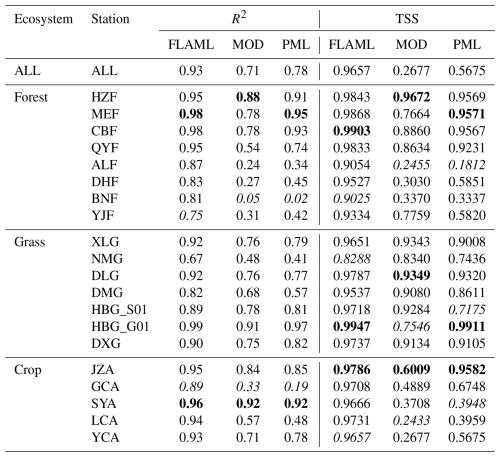
Note that bold numbers indicate the highest values, while italic numbers represent the lowest values.

However, further work is needed to evaluate the FLAML-LUE model's suitability and accuracy, considering its limitations. In particular, it tends to underestimate high GPP and overestimate low GPP. In addition, the model performance in GPP estimation is highly dependent on ecosystem type. Our findings indicated that mixed forests, deciduous broadleaf forests, and agricultural lands had higher prediction accuracies, while grass sites such as alpine scrub and alpine meadows were predicted with large uncertainties, consistent with results from other studies (Wang et al., 2021b; Yuan et al., 2014). This is still a big challenge in accurately estimating GPP.

In general, satellite imagery accurately captures the seasonal leaf phenology of DBF and MF canopies (e.g., spring leaf unfolding and fall senescence). Additionally, the key environmental factors influencing vegetation production during different phenological phases are well defined (Yuan et al., 2014), making them well suited for FLAML-LUE modeling. In contrast, the ambiguous seasonal leaf area changes in EBF and the low variability of GPP in NMG ecosystems result in poorer model performance, and empirical methods struggle to estimate GPP variability in these areas (Tramontana et al., 2016).

Model performance is heavily influenced by the quality of the driver data and the typicality of the flux towers. In this study, meteorological indices are obtained directly from spatially explicit reanalysis products. Remotely sensed variables (e.g., NDVI and EVI, LSWI) serve as proxies for vegetation growth and seasonal changes and are crucial for scaling simulations from site to regional levels. These gridded indices are directly derived from satellite reflectance bands. Large-area EFs can be obtained using LE and H calculations from ERA5 reanalysis data or can be derived using NDVI temperature triangulation (Venturini et al., 2004). LAI, VPD, Pre, and RH can be obtained from ERA5 reanalysis data. Thus, the model can be extended from the site scale to the regional and even global scale. Building on this foundation, we will develop a long-term gridded GPP dataset for China using the FLAML-LUE framework to analyze its spatiotemporal variations over multiple years. This dataset will allow us to investigate long-term GPP trends across different climate zones and vegetation types, as well as their responses to key environmental drivers. By comparing GPP estimates across regions and years, we will also assess model uncertainties and identify potential areas for improvement.

5 Conclusion

In this study, the FLAML-LUE model was developed based on data from 20 flux observation sites across China, integrating the FLAML algorithm with key variables from the LUE model. The results demonstrate that the FLAML-LUE model performs excellently in GPP prediction, accurately simulating both its temporal variations and magnitude, particularly in mixed forests and coniferous forests. The average R² for daily-scale simulations reached 0.92 and 0.91, respectively. Further analysis showed that extending the temporal scale of input data significantly improves model accuracy. In a comparison of models with different variable combinations, it was found that the model driven by EVI outperformed models driven by NDVI and LAI. The model using LSWI as the driving variable performed better than the models with EF, SW, VPD, Pre, and RH as primary variables, with the EVI + LSWI combination yielding the best performance. Additionally, the model's prediction accuracy decreased under high-temperature and high-VPD conditions. However, under drought conditions, the overall prediction accuracy increased, although it decreased at some sites.

In summary, the FLAML-LUE model demonstrates strong applicability and potential for wider application in GPP estimation. It holds promise for scaling from site level to regional or even global levels, contributing to a deeper understanding of carbon cycling processes. However, the model's applicability in unique ecosystems, such as alpine shrublands, remains limited, and its ability to adapt to extreme climate events requires further enhancement. Future work should focus on optimizing the model structure and parameter settings to improve its robustness and generalization across diverse ecological environments.