Isogeometric analysis of the lithosphere under topographic loading: Igalith v1.0.0

This paper presents methods from isogeometric finite-element analysis for numerically solving problems in geoscience involving partial differential equations. In particular, we consider the numerical simulation of shells and plates in the context of isostasy. Earth's lithosphere is modeled as a thin elastic shell or plate floating on the asthenosphere and subject to topographic loads. We demonstrate the computational methods on the isostatic boundary value problem posed on selected geographic locations. For Europe, the computed lithospheric depression is compared with available Mohorovičić depth data. We also perform parameter identification for the effective elastic thickness of the lithosphere, the rock density, and the topographic load that are most plausible to explain the measured depths. An example of simulating the entire lithosphere of the Earth as a spherical shell using multi-patch isogeometric analysis is presented, providing an alternative to spherical harmonics for solving partial differential equations on a spherical domain. The numerical results serve to showcase the features and capabilities of isogeometric methods rather than to provide insightful predictions since a fairly simple model is used for the loading of the lithosphere.

1 Introduction

Finite-element methods have been widely used to compute numerical approximations of solutions to partial differential equations. In standard finite-element methods, the computational domain is subdivided into parts that are images of elementary geometric shapes, called finite elements, on which a number of shape functions are defined. Usually, the shape functions are polynomial functions determined by interpolation conditions on some reference element. Joining together all the elements along with the shape functions yields a finite-element space in which a numerical solution to the problem is sought. It is constructed by finding a linear combination of the shape functions of each element that best approximates the exact solution (Brenner and Scott, 1994; Braess, 2007; Zienkiewicz et al., 2013).

Global C¹ (continuously differentiable) finite-element spaces are required for a conforming discretization of higher-order problems, such as the shell and plate problems considered in this work. The construction of such spaces is generally computationally expensive and requires a lot of degrees of freedom per element. This difficulty has led to various methods for solving the shell and plate equations more efficiently. An example is the non-conforming mixed formulation given by the classical discrete Kirchhoff triangular (DKT) elements (Batoz et al., 1980), where the C¹ condition is imposed only at the nodes of the mesh. Other examples include the use of rotation-free (RF) elements (Oñate and Zárate, 2000), assumed natural deviatoric strain (ANDES) elements (Mostafa et al., 2013), discontinuous Galerkin (DG) methods (Engel et al., 2002), and the Hellan–Herrmann–Johnson (HHJ) method (Neunteufel and Schöberl, 2019). Another way to address the problem is to apply isogeometric finite-element methods (Kiendl et al., 2009), which is the main topic of this work.

Isogeometric analysis (IGA) is a computational paradigm for solving partial differential equations (PDEs) that employs the same shape functions used to describe the domain of the problem to construct finite-element approximations of solutions to the problem. It allows for the integration of finite-element analysis (FEA) with technologies from computer-aided design (CAD). The concept of isogeometric analysis is first presented in the seminal work by Hughes et al. (2005). Standard references on the subject include Cottrell et al. (2009), Buffa and Sangalli (2016), Lyche et al. (2018), Jüttler and Simeon (2015), and van Brummelen et al. (2021).

B-splines and non-uniform rational B-splines (NURBSs) are conventionally used for the shape functions in isogeometric analysis. One advantage of using them for shell and plate problems is the simple construction of C¹ isogeometric spline spaces on a single patch to discretize the equations with fewer degrees of freedom than standard C¹ finite-element methods. However, it is important to also consider multi-patch geometries for problems of practical relevance. Preserving the C¹ continuity along patch interfaces is not a trivial task and has been an active topic of research (Kiendl et al., 2010; Kapl et al., 2015; Collin et al., 2016; Schuß et al., 2019; Farahat et al., 2023a, b). Another feature of isogeometric analysis presented in this paper is the adaptive local refinement using hierarchical B-splines (Vuong et al., 2011; Garau and Vázquez, 2018; Buffa et al., 2022).

We conduct numerical experiments for various geographic locations using the global topography data from Earth2014 (Hirt and Rexer, 2015). A Mohorovičić depth map is available for the European Plate (Grad et al., 2009), which is used to verify the results. Information about the ground truth additionally allows us to estimate unknown parameters of the model via least-square methods constrained by the governing equations. This is applied to identify the spatial distribution of the effective elastic thickness, the density of overlying rock, and the topographic load that are most plausible to explain the measured data for the Mohorovičić depth.

We begin with the description of the mathematical models that are used in this work to derive the equilibrium equations for shells and plates in the context of isostasy. Section 3 introduces isogeometric analysis and the methods used to discretize and numerically solve boundary value problems using B-splines and NURBSs. In Sect. 4, we provide a method to estimate parameters of the model using available real-world data. Application of the methods to selected geographic locations is discussed in Sect. 5, followed by a summary and conclusions in the last section of the paper.

2 Mathematical model of the lithosphere

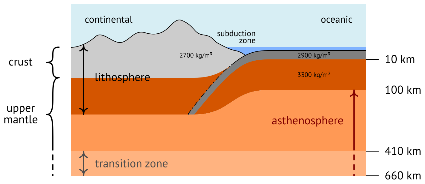
In this work, the term lithosphere refers to the solid part of the Earth's interior that responds elastically to applied mechanical loads on timescales of geologic duration. It encompasses the Earth's outermost layer, the crust, and a portion of the Earth's upper mantle (see Fig. 1). This particular notion is called the elastic lithosphere in Melosh (2011) (Box 3.4) and should be distinguished from the other definitions. Since the mechanical behavior of a planet's interior depends on the rheology of the material of which it is composed and the duration of the loads under consideration, the location and size of the lithosphere are rather ill-defined. Nevertheless, the concept of an elastic lithosphere has proven to be useful for modeling purposes.

We treat the lithosphere as an elastic shell floating on the asthenosphere and subject to gravitational body forces. The asthenosphere comprises the mechanically weak and ductile region of the Earth's upper mantle, which behaves like a viscous fluid on geologic timescales and exerts an outward buoyancy force on the lithosphere. The magnitude of the force is proportional to the pressure difference between the fluid and the submerged body. According to Archimedes' principle, it is equal to the weight of the displaced fluid, which, in our case, depends on the depression of the lithosphere. The weight of topography is treated as a gravitational load; i.e., an inward force proportional to topographic elevation and rock density acts on the lithosphere, which causes its depression. Isostasy or isostatic equilibrium refers to the state of mechanical equilibrium between the lithosphere and the asthenosphere due to gravity and buoyancy (Gutenberg, 1949; Watts, 2001).

In the following, we introduce some basic concepts from the theory of elastic shells and plates to formulate a mathematical model for the lithosphere as described above. For a more elaborate introduction to mathematical elasticity and thin-shell structures, we refer to Marsden and Hughes (1994) and Bischoff et al. (2004), respectively.

Figure 1 Top layers of the Earth (Lowrie, 1997; Rogers, 2008).

2.1 Shell and plate models

A shell is a three-dimensional solid whose thickness in one dimension is considerably small relative to the other two dimensions. The mathematical model of a shell can be reduced to a two-dimensional one by considering only the mechanics on some reference surface (see Fig. 2 for an illustration).

Figure 2 A shell segment and its reference surface (red).

One typically distinguishes between thick- and thin-shell models. Thick-shell models capture transverse shear strains in addition to membrane and bending strains as opposed to thin-shell models, where the shell thickness is assumed to be small enough so that the effects of transverse shear deformations can be neglected. The configuration of a thin shell is fully determined by the position of its reference surface in physical space, whereas the configuration of a thick shell is supplemented by a deformable vector field on the reference surface called a director field.

To showcase the capabilities of isogeometric analysis in solving higher-order problems numerically, we focus on the displacement formulation of the Koiter model for thin shells and the Kirchhoff model for thin plates, which require C¹ finite elements for a conforming discretization. Depending on the ratio of the shell thickness to the scale of the simulation, a thick-shell model might be more adequate for capturing the correct behavior of the lithosphere.

2.1.1 Equilibrium equations for thin elastic shells

Let ℬ denote the shell body, modeled as a three-dimensional manifold consisting of fibers that are transverse to the reference surface 𝒜⊂ℬ. A configuration of ℬ in the physical space ℝ³ is the mapping $\mathit{\xi }:\mathcal{B}\to {\mathbb{R}}^{\mathrm{3}}$, which assigns a spatial point ξ(X)∈ℝ³ to each particle X∈ℬ (see Fig. 3). Under the Kirchhoff–Love assumptions for a thin shell (Love, 1888; Bischoff et al., 2004; Reddy, 2007), any admissible configuration can be locally represented using curvilinear coordinates $\mathit{\vartheta }=({\mathit{\vartheta }}^{\mathrm{1}},{\mathit{\vartheta }}^{\mathrm{2}},{\mathit{\vartheta }}^{\mathrm{3}})$ by means of a mapping of the form

$$\begin{array}{}\text{(1)}& \mathit{\xi }({\mathit{\vartheta }}^{\mathrm{1}},{\mathit{\vartheta }}^{\mathrm{2}},{\mathit{\vartheta }}^{\mathrm{3}})=\mathit{\gamma }({\mathit{\vartheta }}^{\mathrm{1}},{\mathit{\vartheta }}^{\mathrm{2}})+{\mathit{\vartheta }}^{\mathrm{3}}\mathit{n}({\mathit{\vartheta }}^{\mathrm{1}},{\mathit{\vartheta }}^{\mathrm{2}}),\end{array}$$

where γ=ξ|_𝒜 is the mid-surface configuration; n is the unit normal vector field of the reference surface, chosen to be the middle surface of the shell; and ϑ³ is the thickness parameter.

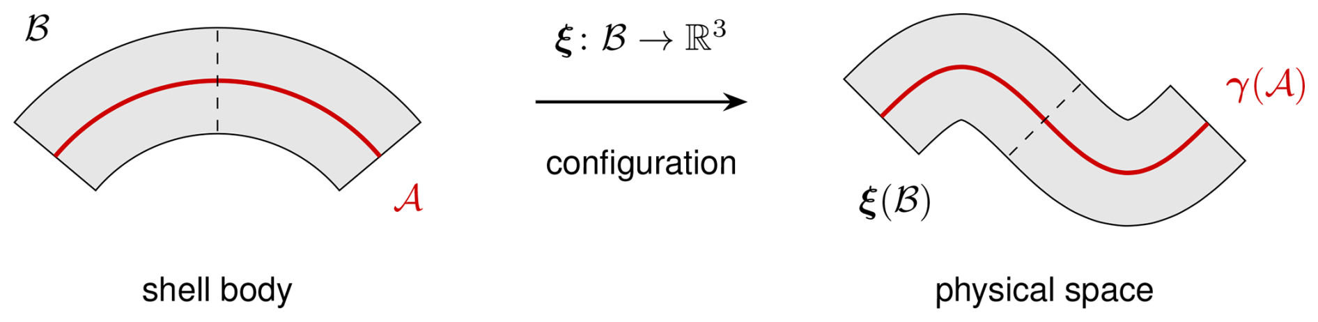
Figure 3 Shell configuration, corresponding mid-surface configuration (red line), and a fiber of the shell (dashed line).

The governing equations for an elastic shell in static equilibrium follow from the principle of virtual work. The total work done on the system is given by the potential energy:

$$\begin{array}{}\text{(2)}& V\left(\mathit{\gamma }\right)=\underset{\mathcal{A}}{\int }W\left(\mathit{E}\right(\mathit{\gamma }\left)\right)\mathrm{dA}-\underset{\mathcal{A}}{\int }{\mathit{F}}_{\mathrm{ext}}\cdot \mathit{\gamma }\mathrm{dA}-\underset{\partial \mathcal{A}}{\int }{\mathit{G}}_{\mathrm{ext}}\cdot \mathit{\gamma }\mathrm{dS},\end{array}$$

where F_ext is an external force acting on the mid-surface 𝒜; G_ext is an external force acting on the boundary ∂𝒜; and W is the stored-energy density function, which depends on the strain tensor E(γ) corresponding to the mid-surface configuration. A shell of Koiter's type has a stored-energy density function that consists of a membrane and a bending part:

$$\begin{array}{}\text{(3)}& W={\displaystyle \frac{\mathrm{1}}{\mathrm{2}}}\left({\mathit{S}}_{\mathrm{m}}:{\mathit{E}}_{\mathrm{m}}+{\mathit{S}}_{\mathrm{b}}:{\mathit{E}}_{\mathrm{b}}\right).\end{array}$$

This can be derived from three-dimensional elasticity by expressing the strain tensor in terms of kinematic variables of the mid-surface and integrating through the thickness t of the shell, assuming a sufficiently thin shell and a small mid-surface strain (Koiter, 1966; Bischoff et al., 2004; Ciarlet, 2005; Steigmann, 2013). The membrane and bending strains are obtained by considering the expansion

$$\begin{array}{}\text{(4)}& \mathit{E}={\mathit{E}}_{\mathrm{m}}+{\mathit{\vartheta }}^{\mathrm{3}}{\mathit{E}}_{\mathrm{b}}+\mathcal{O}\left(\right({\mathit{\vartheta }}^{\mathrm{3}}{)}^{\mathrm{2}})\end{array}$$

and taking the in-plane components, while the effective stress resultants are given by

$$\begin{array}{}\text{(5)}& {\mathit{S}}_{\mathrm{m}}=t\mathit{K}:{\mathit{E}}_{\mathrm{m}},{\mathit{S}}_{\mathrm{b}}={\displaystyle \frac{t^{\mathrm{3}}}{\mathrm{12}}}\mathit{K}:{\mathit{E}}_{\mathrm{b}},\end{array}$$

called the membrane force and the bending moment, respectively. We assume a Saint Venant–Kirchhoff model for linear elastic isotropic materials so that the elasticity tensor reads as

$$\begin{array}{}\text{(6)}& \mathit{K}={\displaystyle \frac{E}{(\mathrm{1}-{\mathit{\nu }}^{\mathrm{2}})}}\left[\begin{array}{ccc}\mathrm{1}& \mathit{\nu }& \mathrm{0}\\ \mathit{\nu }& \mathrm{1}& \mathrm{0}\\ \mathrm{0}& \mathrm{0}& (\mathrm{1}-\mathit{\nu })/\mathrm{2}\end{array}\right]\end{array}$$

in Voigt notation, assuming the vanishing transverse normal stress condition with Young's modulus E and Poisson's ratio ν.

In a state of equilibrium, the virtual work vanishes, and, for any virtual displacement δγ consistent with the constraints imposed on the shell, we have that δV=0 or, equivalently,

$$\begin{array}{}\text{(7)}& \begin{array}{rl}& \underset{\mathcal{A}}{\int }\left({\mathit{S}}_{\mathrm{m}}:\mathit{\delta }{\mathit{E}}_{\mathrm{m}}+{\mathit{S}}_{\mathrm{b}}:\mathit{\delta }{\mathit{E}}_{\mathrm{b}}\right)\mathrm{dA}\\ & =\underset{\mathcal{A}}{\int }{\mathit{F}}_{\mathrm{ext}}\cdot \mathit{\delta }\mathit{\gamma }\mathrm{dA}+\underset{\partial \mathcal{A}}{\int }{\mathit{G}}_{\mathrm{ext}}\cdot \mathit{\delta }\mathit{\gamma }\mathrm{dS}.\end{array}\end{array}$$

The resulting equation is referred to as the weak variational formulation for a Koiter shell in static equilibrium. It is the starting point for the numerical solution of variational problems using finite-element methods.

We consider the displacement field $\mathit{u}=\mathit{\gamma }-{\mathit{\gamma }}_{\mathrm{0}}$ of the mid-surface corresponding to an initial undeformed configuration γ₀ with ${\mathit{E}}_{\mathrm{m}}\left({\mathit{\gamma }}_{\mathrm{0}}\right)={\mathit{E}}_{\mathrm{b}}\left({\mathit{\gamma }}_{\mathrm{0}}\right)=\mathrm{0}$ and replace the strain tensors and corresponding effective stress resultants with

$$\begin{array}{}\text{(8)}& \begin{array}{rl}& {\mathit{e}}_{\mathrm{m}}\left(\mathit{u}\right)=\mathit{\delta }{\mathit{E}}_{\mathrm{m}}({\mathit{\gamma }}_{\mathrm{0}},\mathit{u}),{\mathit{e}}_{\mathrm{b}}\left(\mathit{u}\right)=\mathit{\delta }{\mathit{E}}_{\mathrm{b}}({\mathit{\gamma }}_{\mathrm{0}},\mathit{u}),\\ & {\mathit{s}}_{\mathrm{m}}\left(\mathit{u}\right)=t\mathit{K}:{\mathit{e}}_{\mathrm{m}}\left(\mathit{u}\right),{\mathit{s}}_{\mathrm{b}}\left(\mathit{u}\right)={\displaystyle \frac{t^{\mathrm{3}}}{\mathrm{12}}}\mathit{K}:{\mathit{e}}_{\mathrm{b}}\left(\mathit{u}\right),\end{array}\end{array}$$

to obtain the linear Koiter shell equations (Ciarlet, 2005, Sect. 4.2). The linearized strain tensors in local curvilinear coordinates read as

$$\begin{array}{}\text{(9)}& \begin{array}{rl}& \left[{\mathit{e}}_{\mathrm{m}}\right(\mathit{u}){]}_{\mathit{\alpha }\mathit{\beta }}={\displaystyle \frac{\mathrm{1}}{\mathrm{2}}}({\partial }_{\mathit{\alpha }}\mathit{u}\cdot {\partial }_{\mathit{\beta }}{\mathit{\gamma }}_{\mathrm{0}}+{\partial }_{\mathit{\alpha }}{\mathit{\gamma }}_{\mathrm{0}}\cdot {\partial }_{\mathit{\beta }}\mathit{u}),\\ & \left[{\mathit{e}}_{\mathrm{b}}\right(\mathit{u}){]}_{\mathit{\alpha }\mathit{\beta }}=-{\partial }_{\mathit{\alpha }}{\partial }_{\mathit{\beta }}\mathit{u}\cdot {\mathit{n}}_{\mathrm{0}}-{\partial }_{\mathit{\alpha }}{\partial }_{\mathit{\beta }}{\mathit{\gamma }}_{\mathrm{0}}\cdot \mathit{\delta }\mathit{n},\end{array}\end{array}$$

where $\mathit{\alpha },\mathit{\beta }\in \mathit{\{}\mathrm{1},\mathrm{2}\mathit{\}}$ and $\mathit{\delta }\mathit{n}=\mathit{m}-({\mathit{n}}_{\mathrm{0}}\cdot \mathit{m}){\mathit{n}}_{\mathrm{0}}$, with

$$\begin{array}{}\text{(10)}& {\mathit{n}}_{\mathrm{0}}={\displaystyle \frac{{\partial }_{\mathrm{1}}{\mathit{\gamma }}_{\mathrm{0}}\times {\partial }_{\mathrm{2}}{\mathit{\gamma }}_{\mathrm{0}}}{\Vert {\partial }_{\mathrm{1}}{\mathit{\gamma }}_{\mathrm{0}}\times {\partial }_{\mathrm{2}}{\mathit{\gamma }}_{\mathrm{0}}\Vert }},\mathit{m}={\displaystyle \frac{{\partial }_{\mathrm{1}}\mathit{u}\times {\partial }_{\mathrm{2}}{\mathit{\gamma }}_{\mathrm{0}}+{\partial }_{\mathrm{1}}{\mathit{\gamma }}_{\mathrm{0}}\times {\partial }_{\mathrm{2}}\mathit{u}}{\Vert {\partial }_{\mathrm{1}}{\mathit{\gamma }}_{\mathrm{0}}\times {\partial }_{\mathrm{2}}{\mathit{\gamma }}_{\mathrm{0}}\Vert }}.\end{array}$$

To simplify and fit the problem into an abstract variational framework, we introduce the following notation:

$$\begin{array}{}\text{(11)}& \begin{array}{rl}a(\mathit{u},\mathit{v})& =\underset{\mathcal{A}}{\int }\left({\mathit{s}}_{\mathrm{m}}\left(\mathit{u}\right):{\mathit{e}}_{\mathrm{m}}\left(\mathit{v}\right)+{\mathit{s}}_{\mathrm{b}}\left(\mathit{u}\right):{\mathit{e}}_{\mathrm{b}}\left(\mathit{v}\right)\right)\mathrm{dA},\\ \mathrm{\ell }\left(\mathit{v}\right)& =\underset{\mathcal{A}}{\int }{\mathit{F}}_{\mathrm{ext}}\cdot \mathit{v}\mathrm{dA}+\underset{\partial \mathcal{A}}{\int }{\mathit{G}}_{\mathrm{ext}}\cdot \mathit{v}\mathrm{dS}.\end{array}\end{array}$$

The elastostatic boundary value problem then reads as follows: find an admissible displacement u such that the equation $a(\mathit{u},\mathit{v})=\mathrm{\ell }\left(\mathit{v}\right)$ holds for all admissible variations v=δu.

2.1.2 Reduction to a plate and beam model

In the case where the initial undeformed configuration of the reference surface is planar and where there are no membrane strains, one speaks of a plate instead of a shell. The displacement of the mid-surface from the initial configuration is then reduced to its vertical deflection w perpendicular to the reference plane, e.g., the xy plane, so that

$$\begin{array}{}\text{(12)}& \begin{array}{rl}{\mathit{\gamma }}_{\mathrm{0}}(x,y)& =(x,y,\mathrm{0}),\\ \mathit{\gamma }(x,y)& =(x,y,w(x,y\left)\right),\\ \mathit{u}(x,y)& =(\mathrm{0},\mathrm{0},w(x,y\left)\right).\end{array}\end{array}$$

In this case, the membrane part of the strain tensor vanishes, and the bending term can be written as

$$\begin{array}{}\text{(13)}& {\mathit{s}}_{\mathrm{b}}\left(w\right):{\mathit{e}}_{\mathrm{b}}\left(v\right)=D\left(\mathit{\nu }\mathrm{\Delta }w\mathrm{\Delta }v+(\mathrm{1}-\mathit{\nu }){\mathrm{\nabla }}^{\mathrm{2}}w:{\mathrm{\nabla }}^{\mathrm{2}}v\right),\end{array}$$

where v=δw is now the variation in the vertical direction, and the coefficient

$$\begin{array}{}\text{(14)}& D={\displaystyle \frac{E{t}^{\mathrm{3}}}{\mathrm{12}(\mathrm{1}-{\mathit{\nu }}^{\mathrm{2}})}}\end{array}$$

denotes the flexural rigidity of the plate. The weak formulation for a Kirchhoff plate then reads as

$$\begin{array}{}\text{(15)}& \begin{array}{rl}a(w,v)& =\underset{\mathcal{A}}{\int }D\left(\mathit{\nu }\mathrm{\Delta }w\mathrm{\Delta }v+(\mathrm{1}-\mathit{\nu }){\mathrm{\nabla }}^{\mathrm{2}}w:{\mathrm{\nabla }}^{\mathrm{2}}v\right)\mathrm{dA},\\ \mathrm{\ell }\left(v\right)& =\underset{\mathcal{A}}{\int }{f}_{\mathrm{ext}}v\mathrm{dA}+\underset{\partial \mathcal{A}}{\int }{g}_{\mathrm{ext}}v\mathrm{dS},\end{array}\end{array}$$

where f_ext and g_ext denote the vertical components of F_ext and G_ext, respectively.

In the one-dimensional case with w=w(x), the bending term is reduced further, which leads to a fourth-order differential equation for a Euler–Bernoulli beam when considering the strong formulation of the problem without boundary conditions:

$$\begin{array}{}\text{(16)}& {\displaystyle \frac{{\mathrm{d}}^{\mathrm{2}}}{\mathrm{d}{x}^{\mathrm{2}}}}\left(\stackrel{\mathrm{̃}}{D}{\displaystyle \frac{{\mathrm{d}}^{\mathrm{2}}w}{\mathrm{d}{x}^{\mathrm{2}}}}\right)=f_{\mathrm{ext}}.\end{array}$$

Here, $\stackrel{\mathrm{̃}}{D}$ is another flexural rigidity that depends on the cross-sectional geometry of the beam. Note that additional rotational effects, i.e., torsion in addition to bending, do not occur in the model as a result of assuming a flat initial undeformed configuration with only vertical deflections.

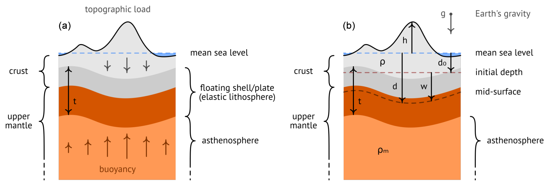
Figure 4 Floating elastic lithosphere under topographic loading (a) and relevant quantities for the mathematical model (b).

2.2 Topographic loading and buoyancy

We model the lithosphere as a thin elastic plate of effective elastic thickness t floating on the asthenosphere and subject to gravitational forces (see Fig. 4a for an illustration). The initial depth of the mid-surface in the undeformed configuration corresponds to the theoretical depth relative to the mean sea level when there is no overlying mass. The actual mid-surface of the lithosphere does not have to coincide with the Mohorovičić surface, which is the boundary between the crust and the upper mantle of the Earth. However, we assume that they are close to each other and differ only by a constant vertical displacement, which is a simplification of the model that disregards subsurface variations, usually obtained via inversion of gravity anomalies.

Starting from the equilibrium equations for a Kirchhoff plate in Sect. 2.1.2 with the external load f_ext, we split up the contributions from gravity and buoyancy: $f_{\mathrm{ext}}=f_{\mathrm{grav}}+f_{\mathrm{buoy}}$.

Gravitational load is obtained by integrating all of the weight above the mid-surface. The density of overlying air is considered to be negligible so that the weight of topography ranges from Earth's surface down to the mid-surface. It is given by

$$\begin{array}{}\text{(17)}& f_{\mathrm{grav}}=-\underset{d}{\overset{h}{\int }}\mathit{\varrho }g\mathrm{d}z,\end{array}$$

where d is the depth of the mid-surface relative to the mean sea level; h is the topographic elevation; ϱ is the density of overlying mass; and g is the gravitational acceleration, which is assumed to be constant for the sake of simplicity.

The vertical displacement of the mid-surface from the initial depth is given by $w=d-d_{\mathrm{0}}$ (see Fig. 4b). The buoyant force is equal to the weight of the displaced asthenosphere; thus

$$\begin{array}{}\text{(18)}& f_{\mathrm{buoy}}=\underset{d}{\overset{d_{\mathrm{0}}}{\int }}{\mathit{\varrho }}_{\mathrm{m}}g\mathrm{d}z=-{\mathit{\varrho }}_{\mathrm{m}}gw,\end{array}$$

assuming a constant upper-mantle density ϱ_m.

Instead of working with the actual topographic elevation, we use a mass representation r obtained by taking the mass above the mid-surface of the lithosphere and normalizing it by some depth-independent reference density ϱ_r. We choose the reference density as the mean rock density from the current depth of the mid-surface to its initial depth and assume that it is homogeneous in space so that

$$\begin{array}{}\text{(19)}& {\mathit{\varrho }}_{\mathrm{r}}={\displaystyle \frac{\mathrm{1}}{\left|w\right|}}\underset{d}{\overset{d_{\mathrm{0}}}{\int }}\mathit{\varrho }\mathrm{d}z,r={\displaystyle \frac{\mathrm{1}}{{\mathit{\varrho }}_{\mathrm{r}}}}\underset{d_{\mathrm{0}}}{\overset{h}{\int }}\mathit{\varrho }\mathrm{d}z.\end{array}$$

Using the mass representation, which corresponds to rock-equivalent topography, we can write the external load as

$$\begin{array}{}\text{(20)}& f_{\mathrm{ext}}=-({\mathit{\varrho }}_{\mathrm{m}}-{\mathit{\varrho }}_{\mathrm{r}})gw-{\mathit{\varrho }}_{\mathrm{r}}gr.\end{array}$$

Plugging this into the weak formulation for the plate model without external boundary forces yields $a(w,v)+b(w,v)=c\left(v\right)$ with the bilinear form in Eq. (15) and

$$\begin{array}{}\text{(21)}& b(w,v)=\underset{\mathcal{A}}{\int }({\mathit{\varrho }}_{\mathrm{m}}-{\mathit{\varrho }}_{\mathrm{r}})gwv\mathrm{dA},c\left(v\right)=-\underset{\mathcal{A}}{\int }{\mathit{\varrho }}_{\mathrm{r}}grv\mathrm{dA}.\end{array}$$

This is the Vening-Meinesz model of flexural isostasy used to explain regional compensation (Vening-Meinesz, 1931; Abd-Elmotaal, 1995; Pelletier, 2008, Chap. 5).

In the case where there is no flexural rigidity, the Vening-Meinesz model is reduced to the Airy–Heiskanen model of local isostasy (Airy, 1855), for which the well-known relation

$$\begin{array}{}\text{(22)}& \left({\displaystyle \frac{{\mathit{\varrho }}_{\mathrm{m}}-{\mathit{\varrho }}_{\mathrm{r}}}{{\mathit{\varrho }}_{\mathrm{r}}}}\right)(d_{\mathrm{0}}-d)=r\end{array}$$

holds. It states that the lithospheric depression relative to the initial depth is proportional to the mass representation of the topography with a scaling factor of $({\mathit{\varrho }}_{\mathrm{m}}-{\mathit{\varrho }}_{\mathrm{r}})/{\mathit{\varrho }}_{\mathrm{r}}$. Using the above relation, we can determine the initial depth from some standard crustal thickness t₀ corresponding to a lithospheric plate in local isostasy when the topographic elevation is zero.

2.3 Isostatic boundary value problem

If we consider only a portion of Earth's lithosphere for the simulation, conditions on the boundary of the domain have to be prescribed to compensate for the missing information outside of it. A natural choice is given by the full Neumann boundary condition, which corresponds to setting g_ext=0 on the whole boundary. The resulting isostatic boundary value problem for the plate model then reads as follows: find an admissible deflection w such that $a(w,v)+b(w,v)=c\left(v\right)$ for all admissible variations v=δw.

The Sobolev space H²(𝒜) is chosen as the space of admissible deflections for the boundary value problem. It consists of square-integrable functions on the reference surface with square-integrable weak derivatives up to the second order. For the full Neumann problem, the variational problem is well-posed by the Lax–Milgram theorem (Braess, 2007, Chap. II), provided that 𝒜⊂ℝ² is a bounded Lipschitz domain and the coefficients D(1−ν) and (ϱ_m−ϱ_r)g are bounded from below by a positive number. The H² coercivity of the bilinear form follows from the fact that the H² norm is equivalent to a similar one without the terms containing first-order derivatives (Nečas, 2012, Theorem 1.8).

The above displacement formulation requires H² regularity, which implies global C¹ continuity for the trial and test functions. The difficulty of C¹ finite elements can be circumvented by considering isogeometric shape functions.

2.4 Spherical model of the lithosphere

Using the more general shell equations, it is possible to perform simulations of the lithosphere on the whole surface of the Earth. From a modeling point of view, the results may not reflect the physical reality since the Earth consists of different regimes and tectonic plates that interact with each other in a complex manner. Furthermore, due to the large scale of the simulation, the effects of flexural rigidity will not be visible. Nevertheless, we assume that the entire lithosphere can be modeled as a single spherical shell to showcase the capabilities of isogeometric analysis in numerical simulations on curved domains, especially a spherical domain. Note that it is also possible to model the surface of the Earth as an oblate spheroid or an irregular geoid instead of a sphere using isogeometric analysis. For the sake of simplicity, we restrict ourselves to the spherical model in this paper.

Some considerations in Sect. 2.2 for lithospheric plates in isostatic equilibrium have to be adapted to the shell model. The buoyant force in three dimensions reads as

$$\begin{array}{}\text{(23)}& b(\mathit{u},\mathit{v})=\underset{\mathcal{A}}{\int }({\mathit{\varrho }}_{\mathrm{m}}-{\mathit{\varrho }}_{\mathrm{r}})g(\mathit{n}\cdot \mathit{u})(\mathit{n}\cdot \mathit{v})\mathrm{dA},\end{array}$$

where (n⋅u) and (n⋅v) are the radial parts of the trial and test functions, respectively, given by the orthogonal projection onto the unit normal n of the sphere. Similarly, the external load is given by a radial gravitational force

$$\begin{array}{}\text{(24)}& c\left(\mathit{v}\right)=-\underset{\mathcal{A}}{\int }{\mathit{\varrho }}_{\mathrm{r}}gr(\mathit{n}\cdot \mathit{v})\mathrm{dA}.\end{array}$$

With the above adjustments, the isostatic problem for a Koiter shell then reads as follows: find an admissible displacement u such that $a(\mathit{u},\mathit{v})+b(\mathit{u},\mathit{v})=c\left(\mathit{v}\right)$ holds for all admissible variations v=δu. We consider the vector-valued Sobolev space H²(𝒜)³ for the displacements of the spherical shell.

3 Isogeometric finite-element analysis

Isogeometric analysis (IGA) is a computational approach for solving partial differential equations (PDEs) numerically that employs non-uniform rational basis splines (NURBSs) to both parameterize the domain and construct finite-element approximations of solutions to the corresponding partial differential equations. This section introduces the notions required for the numerical discretization of elliptic boundary value problems using isogeometric analysis, particularly the isostatic boundary value problem. We begin with the definition of B-splines and NURBSs. A more elaborate treatment of NURBSs with numerical algorithms can be found in Rogers (2001), Cohen et al. (2001), de Boor (1978), Schneider (1996), and the NURBS book (Piegl and Tiller, 1995).

3.1 B-splines and NURBSs

Let ${\mathit{\vartheta }}_{\mathrm{0}}\le \mathrm{\cdots }\le {\mathit{\vartheta }}_m$ be a finite sequence of non-decreasing real numbers. A spline of degree p is a piecewise polynomial function $f:[{\mathit{\vartheta }}_{\mathrm{0}},{\mathit{\vartheta }}_m]\to \mathbb{R}$, with the property that the restriction to each subinterval $[{\mathit{\vartheta }}_{i-\mathrm{1}},{\mathit{\vartheta }}_i)$ for $i=\mathrm{1},\mathrm{\dots },m$ is a polynomial function of maximum degree p. The tuple $\mathbf{\Theta }=({\mathit{\vartheta }}_{\mathrm{0}},\mathrm{\dots },{\mathit{\vartheta }}_m)$ is called a knot sequence for the spline with knot values ϑ_i, and the term breakpoint is used to refer to a distinct knot value. The half-open interval $[{\mathit{\vartheta }}_{i-\mathrm{1}},{\mathit{\vartheta }}_i)$ is called the ith knot span, which can be empty.

The maximum order of continuity that a spline of degree p can attain at the breakpoints is p−1. We refer to such splines as smooth splines. A lower order of continuity can be obtained by placing multiple knots at the same location. Each additional knot reduces the order of continuity by 1 until the resulting spline is discontinuous at the breakpoint.

The type of a spline is completely characterized by its degree and the knot sequence. Let 𝒮(Θ,p) denote the space of splines of degree p with knot sequence Θ. It is a vector space of dimension m−p. By introducing the numbers $\stackrel{\mathrm{̃}}{m}=m+\mathrm{1}$, $\stackrel{\mathrm{̃}}{p}=p+\mathrm{1}$, and $\stackrel{\mathrm{̃}}{n}=n+\mathrm{1}$, where $\stackrel{\mathrm{̃}}{m}$ is the number of knots, $\stackrel{\mathrm{̃}}{p}$ is the order of the spline, and $\stackrel{\mathrm{̃}}{n}$ is the dimension of 𝒮(Θ,p), we can write $\stackrel{\mathrm{̃}}{n}=\stackrel{\mathrm{̃}}{m}-\stackrel{\mathrm{̃}}{p}$ or, equivalently, $m=n+p+\mathrm{1}$.

In the following, we consider splines on the unit interval [0,1] with an open knot sequence – i.e., the first and last knot values have multiplicity p+1 – to enable interpolatory control points at the boundary. Thus, the knot sequence has the form

$$\begin{array}{}\text{(25)}& \mathbf{\Theta }=(\underset{(p+\mathrm{1})\text{-times}}{\underbrace{\mathrm{0},\mathrm{\dots },\mathrm{0}}},{\mathit{\vartheta }}_{p+\mathrm{1}},\mathrm{\dots },{\mathit{\vartheta }}_n,\underset{(p+\mathrm{1})\text{-times}}{\underbrace{\mathrm{1},\mathrm{\dots },\mathrm{1}}}),\end{array}$$

where we have ${\mathit{\vartheta }}_{\mathrm{0}}=\mathrm{\cdots }={\mathit{\vartheta }}_p=\mathrm{0}$, ${\mathit{\vartheta }}_{n+\mathrm{1}}=\mathrm{\cdots }={\mathit{\vartheta }}_{n+p+\mathrm{1}}=\mathrm{1}$, and ${\mathit{\vartheta }}_i\in (\mathrm{0},\mathrm{1})$ for $i=p+\mathrm{1},\mathrm{\dots },n$.

3.1.1 B-spline basis functions

A particular basis for the spline space 𝒮(Θ,p) is given by the B-splines (basis splines). They have minimal support and allow for quick evaluation of the splines using de Boor's algorithm, which is convenient for isogeometric analysis. The B-splines of degree p are recursively defined via the Cox–de Boor formula,

$$\begin{array}{}\text{(26)}& \begin{array}{rl}{B}_{k,p}\left(\mathit{\vartheta }\right)& ={\displaystyle \frac{\mathit{\vartheta }-{\mathit{\vartheta }}_k}{{\mathit{\vartheta }}_{k+p}-{\mathit{\vartheta }}_k}}{B}_{k,p-\mathrm{1}}\left(\mathit{\vartheta }\right)\\ & +{\displaystyle \frac{{\mathit{\vartheta }}_{k+\mathrm{1}+p}-\mathit{\vartheta }}{{\mathit{\vartheta }}_{k+\mathrm{1}+p}-{\mathit{\vartheta }}_{k+\mathrm{1}}}}{B}_{k+\mathrm{1},p-\mathrm{1}}\left(\mathit{\vartheta }\right),\end{array}\end{array}$$

with $\mathit{\vartheta }\in [\mathrm{0},\mathrm{1}]$, $k=\mathrm{0},\mathrm{\dots },n$, and

$$\begin{array}{}\text{(27)}& B_{k,\mathrm{0}}\left(\mathit{\vartheta }\right)=\left\{\begin{array}{ll}\mathrm{1}& \text{for }\mathit{\vartheta }\in [{\mathit{\vartheta }}_k,{\mathit{\vartheta }}_{k+\mathrm{1}}),\\ \mathrm{0}& \text{otherwise},\end{array}\right.\end{array}$$

for $k=\mathrm{0},\mathrm{\dots },n+p$, where the convention $\mathrm{0}/\mathrm{0}=\mathrm{0}$ is used if the knot values in the denominator coincide. We refer to B_k,p as the kth B-spline basis function of degree p.

Given a finite sequence of control points ${\mathit{c}}_{\mathrm{0}},\mathrm{\dots },{\mathit{c}}_n\in {\mathbb{R}}^r$ in the physical space of dimension r, we can construct a B-spline curve of degree p through a linear combination of the form

$$\begin{array}{}\text{(28)}& \mathit{\gamma }:[\mathrm{0},\mathrm{1}]\to {\mathbb{R}}^r,\mathit{\gamma }\left(\mathit{\vartheta }\right)=\sum _{k=\mathrm{0}}^n{\mathit{c}}_k{B}_{k,p}\left(\mathit{\vartheta }\right).\end{array}$$

B-spline curves are commonly used to represent shapes in computer-aided geometric design (CAGD). The description using control points allows for intuitive local manipulation of free-form shapes. In isogeometric analysis, the control points additionally serve as degrees of freedom for the unknowns in a discretized system of equations.

If the domain of the problem is two- or three-dimensional, B-spline surfaces or volumes are used to describe its geometry. Multivariate spline spaces are constructed via the tensor product of univariate spline spaces. Instead of a single knot sequence and a single spline degree, we have a family of knot sequences $\mathbf{\Theta }=({\mathbf{\Theta }}^{\left(\mathrm{1}\right)},\mathrm{\dots },{\mathbf{\Theta }}^{\left(d\right)})$, along with a tuple of spline degrees $\mathit{p}=(p_{\mathrm{1}},\mathrm{\dots },p_d)$ corresponding to each parametric dimension. The B-spline basis functions of the spline space ${\mathcal{S}}_d(\mathbf{\Theta },\mathit{p})=\mathcal{S}({\mathbf{\Theta }}^{\left(\mathrm{1}\right)},p_{\mathrm{1}})\otimes \mathrm{\cdots }\otimes \mathcal{S}({\mathbf{\Theta }}^{\left(d\right)},p_d)$ are given by

$$\begin{array}{}\text{(29)}& B_{\mathit{k},\mathit{p}}\left(\mathit{\vartheta }\right)=B_{k_{\mathrm{1}},p_{\mathrm{1}}}^{\left(\mathrm{1}\right)}\left({\mathit{\vartheta }}^{\mathrm{1}}\right)\mathrm{\cdots }{B}_{k_d,p_d}^{\left(d\right)}\left({\mathit{\vartheta }}^d\right)\end{array}$$

for $\mathit{\vartheta }=({\mathit{\vartheta }}^{\mathrm{1}},\mathrm{\dots },{\mathit{\vartheta }}^d)\in [\mathrm{0},\mathrm{1}{]}^d$ in the multivariate setting. The B-splines $B_{\mathrm{0},p_j}^{\left(j\right)},\mathrm{\dots },B_{n_j,p_j}^{\left(j\right)}$ form a basis for 𝒮(Θ^(j),p_j), and $\mathit{k}=(k_{\mathrm{1}},\mathrm{\dots },k_d)$ is a multi-index with $k_j=\mathrm{0},\mathrm{\dots },n_j$ for $j=\mathrm{1},\mathrm{\dots },d$. We order the basis functions lexicographically so that B_k,p corresponds to the kth basis function when using an integer index $k=\mathrm{0},\mathrm{\dots },n$ instead of a multi-index.

A d-variate B-spline patch corresponding to the control points ${\mathit{c}}_{\mathrm{0}},\mathrm{\dots },{\mathit{c}}_n\in {\mathbb{R}}^r$ is a parameterization of the form

$$\begin{array}{}\text{(30)}& \mathit{\gamma }:[\mathrm{0},\mathrm{1}{]}^d\to {\mathbb{R}}^r,\mathit{\gamma }(\mathit{\vartheta })=\sum _{k=\mathrm{0}}^n{\mathit{c}}_k{B}_{k,\mathit{p}}(\mathit{\vartheta }).\end{array}$$

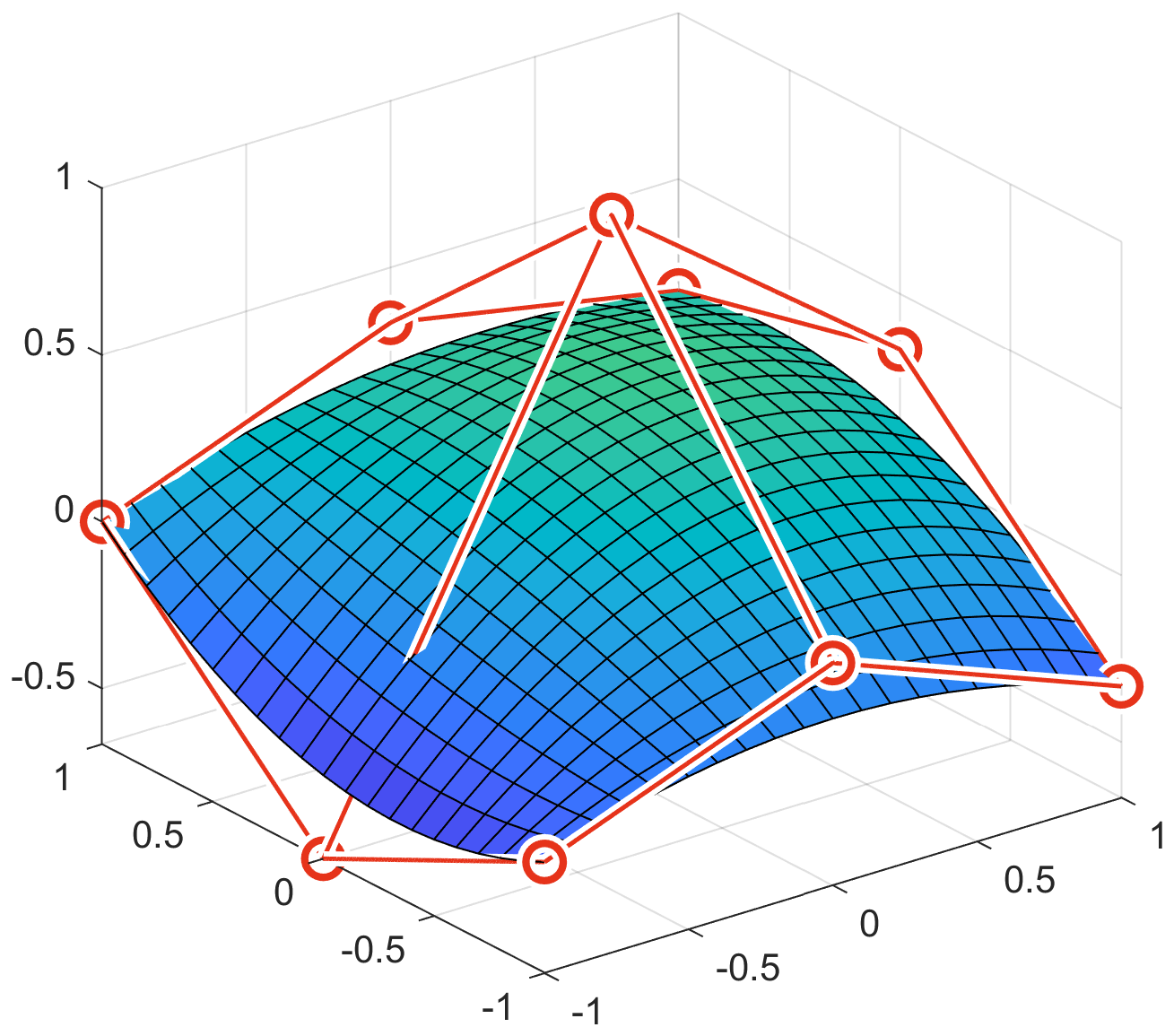
We also refer to the image of γ as a B-spline patch and write ${\mathcal{S}}_{d,r}(\mathbf{\Theta },\mathit{p})$ for the space of d-variate B-spline patches in ℝ^r. See Fig. 6 for an example of a B-spline function on a biquadratic B-spline patch.

Figure 5 Isogeometric shape functions on a biquadratic B-spline patch.

Figure 6 Linear combination of the isogeometric shape functions in Fig. 5 and corresponding mesh of control points (red).

3.1.2 NURBS basis functions

B-splines can be generalized to include rational functions in addition to polynomial ones by assigning a weight to each control point. This greatly increases the design capabilities of free-form shapes; e.g., conic sections can be exactly represented by rational B-splines with weighted control points as opposed to non-rational ones. The term non-uniform in the acronym NURBS stresses the fact that the distribution of knot values in the knot sequence is not necessarily uniform.

Given a B-spline basis $B_{\mathrm{0},p},\mathrm{\dots },B_{n,p}$ for the spline space 𝒮(Θ,p) and a tuple of positive weights $\mathit{\omega }=({\mathit{\omega }}_{\mathrm{0}},\mathrm{\dots },{\mathit{\omega }}_n)$, the NURBS space 𝒮^ω(Θ,p) is generated by rational functions of the form

$$\begin{array}{}\text{(31)}& N_{k,p}^{\mathit{\omega }}\left(\mathit{\vartheta }\right)={\displaystyle \frac{{\mathit{\omega }}_k{B}_{k,p}\left(\mathit{\vartheta }\right)}{\mathit{\omega }\left(\mathit{\vartheta }\right)}},k=\mathrm{0},\mathrm{\dots },n,\end{array}$$

with $\mathit{\vartheta }\in [\mathrm{0},\mathrm{1}]$. The weight function in the denominator is a weighted sum of the B-spline basis functions:

$$\begin{array}{}\text{(32)}& \mathit{\omega }\left(\mathit{\vartheta }\right)=\sum _{k=\mathrm{0}}^n{\mathit{\omega }}_k{B}_{k,p}\left(\mathit{\vartheta }\right).\end{array}$$

Note that the original spline space is a special case of the NURBS space with constant weights. For the multivariate case, we proceed similarly to the non-rational B-splines and define the NURBS basis functions as

$$\begin{array}{}\text{(33)}& N_{k,\mathit{p}}^{\mathit{\omega }}\left(\mathit{\vartheta }\right)={\displaystyle \frac{{\prod }_{j=\mathrm{1}}^d{\mathit{\omega }}_{k_j}^{\left(j\right)}{B}_{k_j,p_j}^{\left(j\right)}\left({\mathit{\vartheta }}^j\right)}{\mathit{\omega }\left(\mathit{\vartheta }\right)}},k=\mathrm{0},\mathrm{\dots },n\end{array}$$

for $\mathit{\vartheta }=({\mathit{\vartheta }}^{\mathrm{1}},\mathrm{\dots },{\mathit{\vartheta }}^d)\in [\mathrm{0},\mathrm{1}{]}^d$. The multivariate weight function reads as

$$\begin{array}{}\text{(34)}& \mathit{\omega }\left(\mathit{\vartheta }\right)=\sum _{k_{\mathrm{1}}=\mathrm{0}}^{n_{\mathrm{1}}}\mathrm{\cdots }\sum _{k_d=\mathrm{0}}^{n_d}{\mathit{\omega }}_{k_{\mathrm{1}}}^{\left(\mathrm{1}\right)}{B}_{k_{\mathrm{1}},p_{\mathrm{1}}}^{\left(\mathrm{1}\right)}\left({\mathit{\vartheta }}^{\mathrm{1}}\right)\mathrm{\cdots }{\mathit{\omega }}_{k_d}^{\left(d\right)}{B}_{k_d,p_d}^{\left(d\right)}\left({\mathit{\vartheta }}^d\right),\end{array}$$

where $\mathit{\omega }=({\mathit{\omega }}^{\left(\mathrm{1}\right)},\mathrm{\dots },{\mathit{\omega }}^{\left(d\right)})$ is a family of weight tuples corresponding to each parametric dimension. Contrarily to non-rational B-splines, the resulting multivariate NURBS space ${\mathcal{S}}_d^{\mathit{\omega }}(\mathbf{\Theta },\mathit{p})$ is no longer a tensor-product space because of the weight function ω. Nevertheless, it is called tensor-product-like, following the terminology in isogeometric analysis.

A d-variate NURBS patch corresponding to the control points ${\mathit{c}}_{\mathrm{0}},\mathrm{\dots },{\mathit{c}}_n\in {\mathbb{R}}^r$ is a parameterization of the form

$$\begin{array}{}\text{(35)}& \mathit{\gamma }:[\mathrm{0},\mathrm{1}{]}^d\to {\mathbb{R}}^r,\mathit{\gamma }(\mathit{\vartheta })=\sum _{k=\mathrm{0}}^n{\mathit{c}}_k{N}_{k,\mathit{p}}^{\mathit{\omega }}(\mathit{\vartheta }).\end{array}$$

We also refer to the image of γ as a NURBS patch and write ${\mathcal{S}}_{d,r}^{\mathit{\omega }}(\mathbf{\Theta },\mathit{p})$ for the space of d-variate NURBS patches in ℝ^r.

To shorten the notation, we omit the superscript ω and the subscript p from the NURBS basis functions and introduce the double index $\mathit{\alpha }=(k,l)$, ranging from (0,1) to (n,r), so that a NURBS patch can be written as

$$\begin{array}{}\text{(36)}& \mathit{\gamma }=\sum _{k=\mathrm{0}}^n\sum _{l=\mathrm{1}}^r{c}_{k,l}{N}_k{\mathit{e}}_l=\sum _{k=\mathrm{0}}^n\sum _{l=\mathrm{1}}^r{c}_{k,l}{\mathit{N}}_{k,l}=\sum _{\mathit{\alpha }\in \mathfrak{A}}{c}_{\mathit{\alpha }}{\mathit{N}}_{\mathit{\alpha }},\end{array}$$

where $\mathfrak{A}=\left\{(k,l)\in {\mathbb{N}}_{\mathrm{0}}^{\mathrm{2}}\mid \mathrm{0}\le k\le n,\mathrm{1}\le l\le r\right\}$ is the index set with $(n+\mathrm{1})\cdot r$ elements, $c_{\mathit{\alpha }}=c_{k,l}$ is the lth component of the kth control point, and ${\mathit{N}}_{\mathit{\alpha }}={\mathit{N}}_{k,l}=N_k{\mathit{e}}_l$ is the αth vector-valued NURBS basis function.

3.1.3 Refinement methods

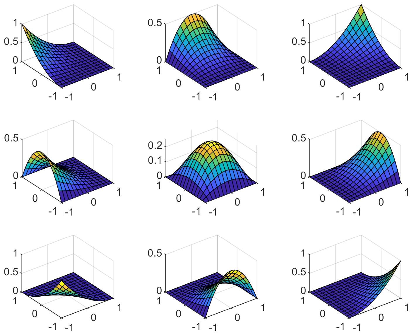
In order to get better approximation results for the numerical solutions, the NURBS space used for the discretization of the problem has to be refined. There are two refinement methods that increase the number of shape functions and maintain the global smoothness of the NURBS space. The first method is called knot insertion, also known as h refinement, where a finer NURBS space is constructed by adding new breakpoints to the knot sequence. The second one is order elevation, or p refinement, which raises the order of the NURBS space without changing the knot spans. Performing order elevation followed by knot insertion results in a so-called k refinement. See Fig. 7 for an illustration of the methods.

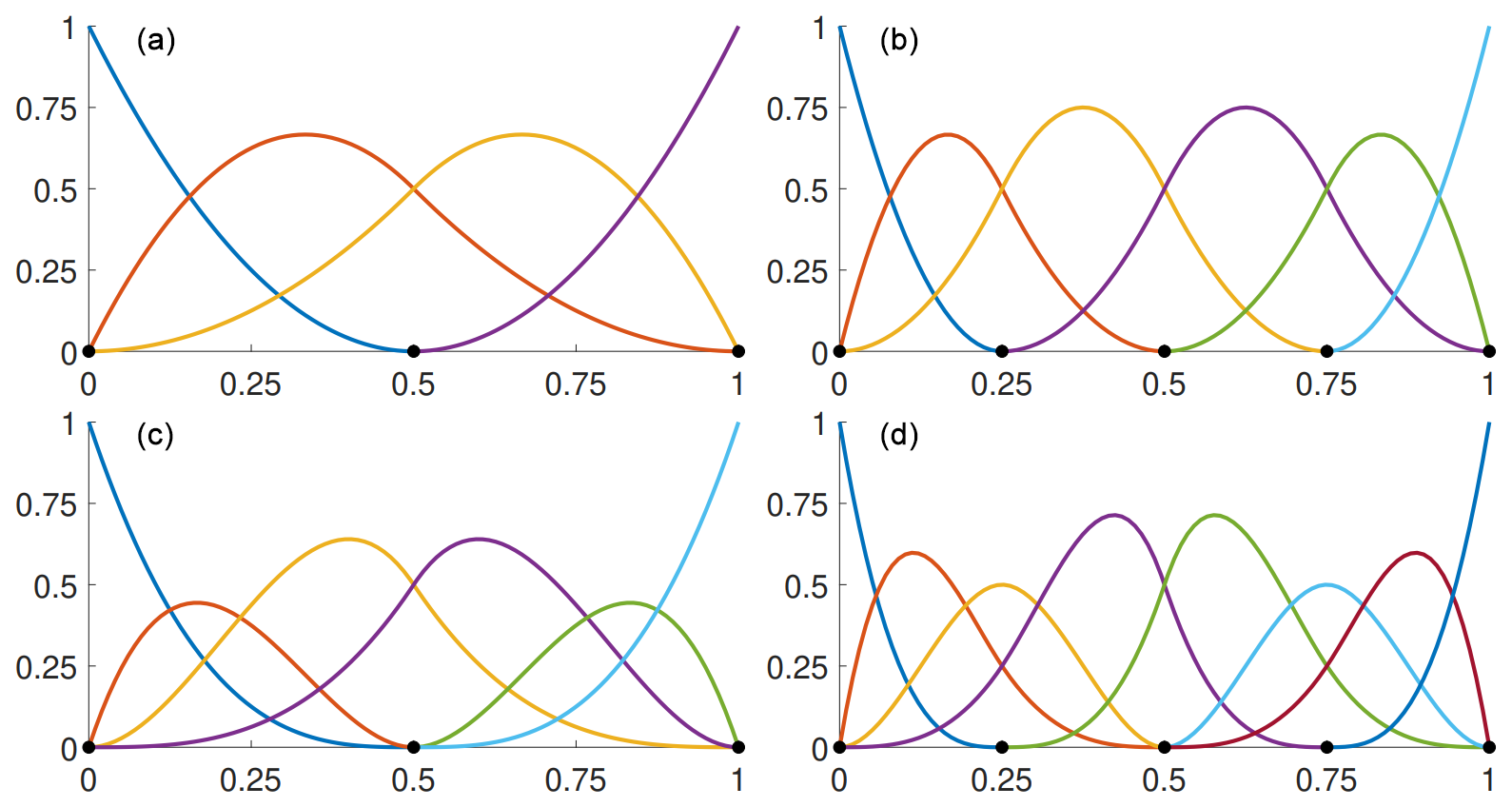
Figure 7 Initial isogeometric shape functions (quadratic B-splines, a) and the shape functions that result from h refinement (b), p refinement (c), and k refinement (d).

For the multivariate case, inserting a breakpoint into a knot sequence will affect all elements along the transverse direction due to the tensor-product-like structure. To enable local refinement, several methods can be considered. In our work, we employ hierarchical B-splines as described in Vuong et al. (2011). Adaptive local refinement can then be performed if an error estimator for the numerical solution to the problem is available (Garau and Vázquez, 2018; Buffa et al., 2022).

3.2 Isogeometric discretization

Given a weak formulation of the variational problem, a numerical solution can be obtained by considering a projection onto some finite-dimensional subspace of the solution space. This is generally referred to as a Galerkin projection. Finite-element methods are based on subdividing the domain of the problem into a finite number of elements, on which a number of shape functions are defined. The finite-element space is then constructed from linear combinations of the shape functions of each element that satisfy certain interpolation conditions.

Isoparametric finite elements enable the solution of problems on domains with curved boundaries by using the same shape functions for the numerical approximation of solutions to describe the geometry of the domain. They serve as a basis for the isogeometric paradigm, where we consider domains that can be represented by some NURBS geometry and use refinements of the corresponding NURBS space to construct approximations of solutions to the problem.

An isogeometric mesh consists of NURBS patches, each of which can be refined to increase the accuracy of the numerical approximation. As opposed to a standard finite-element mesh, the smoothness of shape functions within each patch can be preserved without much effort when the mesh is subdivided into smaller elements. This greatly reduces the number of degrees of freedom compared to classical C¹ finite elements, which is useful when working with shell and plate equations that require global C¹ continuity.

We first consider domains that can be exactly represented by a single NURBS patch. The main idea is to transform the problem posed on the patch to a fixed parameter domain to approximate the solution with a linear combination of NURBS functions that result from refinements of the NURBS space associated with the geometry function and transform the numerical solution back to the physical domain.

3.2.1 Domain transformation

Let Ω⊂ℝ^r denote the physical domain described by the geometry function

$$\begin{array}{}\text{(37)}& {\mathit{\gamma }}_{\mathrm{0}}:\widehat{\mathrm{\Omega }}\to \mathrm{\Omega },{\mathit{\gamma }}_{\mathrm{0}}\left(\mathit{\vartheta }\right)=\sum _{k=\mathrm{0}}^n\sum _{l=\mathrm{1}}^r{G}_{k,l}{\mathit{N}}_{k,l}\left(\mathit{\vartheta }\right),\end{array}$$

with control points ${\mathit{G}}_{\mathrm{0}},\mathrm{\dots },{\mathit{G}}_n\in {\mathbb{R}}^r$ and the parameter domain $\widehat{\mathrm{\Omega }}=[\mathrm{0},\mathrm{1}{]}^d$. To ensure that the domain is suitable for isogeometric analysis, we require that the geometry function is at least a bi-Lipschitz transformation. Thus, it is important to impose conditions on the control points of the geometry such that this requirement is fulfilled.

The weak formulation of a variational problem posed on the physical domain can be transformed to the parameter domain by pulling back functions in the solution space 𝒱(Ω) to the parameter domain using the geometry function. By doing so, we obtain an equivalent weak formulation of the problem posed on the parameter domain: find $\widehat{\mathit{u}}\in \widehat{\mathcal{V}}\left(\widehat{\mathrm{\Omega }}\right)$ such that $\widehat{a}(\widehat{\mathit{u}},\widehat{\mathit{v}})=\widehat{\mathrm{\ell }}\left(\widehat{\mathit{v}}\right)$ for all $\widehat{\mathit{v}}\in \widehat{\mathcal{V}}\left(\widehat{\mathrm{\Omega }}\right)$, with $\widehat{\mathcal{V}}\left(\widehat{\mathrm{\Omega }}\right)=\mathit{\{}\mathit{v}\circ {\mathit{\gamma }}_{\mathrm{0}}\mid \mathit{v}\in \mathcal{V}(\mathrm{\Omega }\left)\mathit{\right\}}$ and

$$\begin{array}{}\text{(38)}& \widehat{a}(\widehat{\mathit{u}},\widehat{\mathit{v}})=a(\widehat{\mathit{u}}\circ {\mathit{\gamma }}_{\mathrm{0}}^{-\mathrm{1}},\widehat{\mathit{v}}\circ {\mathit{\gamma }}_{\mathrm{0}}^{-\mathrm{1}}),\widehat{\mathrm{\ell }}\left(\widehat{\mathit{v}}\right)=\mathrm{\ell }(\widehat{\mathit{v}}\circ {\mathit{\gamma }}_{\mathrm{0}}^{-\mathrm{1}}).\end{array}$$

3.2.2 Ritz–Galerkin method

To discretize the transformed weak formulation, we consider isogeometric shape functions that result from refinements of the NURBS space associated with the geometry function. We choose ${\widehat{\mathcal{V}}}_{h,p}={\mathcal{S}}_{d,s}^{\mathit{\omega }}({\mathbf{\Theta }}_h,\mathit{p})\cap \widehat{\mathcal{V}}\left(\widehat{\mathrm{\Omega }}\right)$ for the finite-dimensional subspace, where h is a discretization parameter corresponding to the diameter of elements, and s is the number of components of functions in the solution space. Galerkin projection then yields a family of finite-dimensional problems of the following form: find ${\widehat{\mathit{u}}}_{h,p}\in {\widehat{\mathcal{V}}}_{h,p}$ such that $\widehat{a}({\widehat{\mathit{u}}}_{h,p},{\widehat{\mathit{v}}}_{h,p})=\widehat{\mathrm{\ell }}\left({\widehat{\mathit{v}}}_{h,p}\right)$ for all ${\widehat{\mathit{v}}}_{h,p}\in {\widehat{\mathcal{V}}}_{h,p}$.

The trial and test functions are now given by linear combinations of the NURBS basis functions; i.e.,

$$\begin{array}{}\text{(39)}& {\widehat{\mathit{u}}}_{h,p}=\sum _{k=\mathrm{0}}^n\sum _{l=\mathrm{1}}^s{U}_{k,l}{\mathit{N}}_{k,l},{\widehat{\mathit{v}}}_{h,p}=\sum _{k=\mathrm{0}}^n\sum _{l=\mathrm{1}}^s{V}_{k,l}{\mathit{N}}_{k,l},\end{array}$$

with control points ${\mathit{U}}_{\mathrm{0}},\mathrm{\dots },{\mathit{U}}_n\in {\mathbb{R}}^s$ and ${\mathit{V}}_{\mathrm{0}},\mathrm{\dots },{\mathit{V}}_n\in {\mathbb{R}}^s$, respectively. The coordinates of the control points are organized in a single column vector so that the Galerkin equation can be written in matrix–vector form. The problem is then reduced to solving a system of linear equations of the form A^TU=L with the coefficient matrix $A_{\mathit{\alpha }\mathit{\beta }}=\widehat{a}({\mathit{N}}_{\mathit{\alpha }},{\mathit{N}}_{\mathit{\beta }})$ and the right-hand-side $L_{\mathit{\beta }}=\widehat{\mathrm{\ell }}\left({\mathit{N}}_{\mathit{\beta }}\right)$, where α and β are double indices in some specified order, ranging from (0,1) to (n,s).

The solution vector $\mathit{U}\in {\mathbb{R}}^{(n+\mathrm{1})s}$ contains the coordinates of the control points associated with the trial function ${\widehat{\mathit{u}}}_{h,p}$ and is referred to as the vector of degrees of freedom in the fully unconstrained solution space. When boundary or interface conditions are present, it is restricted to a subspace fulfilling those conditions.

3.2.3 Multi-patch C¹ coupling

In the case where the domain consists of multiple NURBS patches, the subproblems on each patch have to be coupled in a way that maintains the global C¹ continuity of solutions. There are various methods that can be employed to achieve this in the context of isogeometric analysis of plates and shells. Penalty methods (Kiendl et al., 2010; Coradello et al., 2021a, b), Nitsche methods (Apostolatos et al., 2014; Nguyen et al., 2014; Guo and Ruess, 2015), and mortar methods (Dornisch et al., 2015; Bouclier et al., 2017; Horger et al., 2019) fall into the category of weak-coupling methods that use a modified variational formulation to establish the C¹ continuity weakly across multiple patches. Strong-coupling methods, on the other hand, are based on the construction of global C¹ shape functions, which are then used for a C¹-conforming discretization of the variational formulation. Multi-patch C¹ isogeometric spline spaces can be constructed by replacing shape functions that influence the derivative of solutions at patch interfaces with C¹ shape functions that cover multiple patches (Kapl et al., 2017a, b). This has been extended from the case of planar multi-patch domains to multi-patch surfaces in Farahat et al. (2023a, b). Another approach to stitch shape functions at patch interfaces together is to impose the C¹ condition at some collocation points (Chan et al., 2018) or weakly via the constraint matrix

$$\begin{array}{}\text{(40)}& C_{\mathit{\alpha }\mathit{\beta }}=\underset{\mathrm{\Gamma }}{\int }\left[\right[\mathit{n}\cdot \mathrm{\nabla }{\mathit{N}}_{\mathit{\alpha }}\left]\right]\left[\right[\mathit{n}\cdot \mathrm{\nabla }{\mathit{N}}_{\mathit{\beta }}\left]\right]\mathrm{dS},\end{array}$$

where n is a unit normal at the patch interface Γ, and [[⋅]] denotes the jump of a function between the patches (Collin et al., 2016). The latter yields an approximately C¹ isogeometric spline space on a multi-patch geometry (Weinmüller and Takacs, 2022) and has been used for the numerical experiments in this work. The method is straightforward to implement but has the drawback that the resulting system of linear equations will lose its sparse structure if the basis functions for the null space of the constraint matrix are not carefully chosen to be locally supported. Note that contiguous patches are assumed to share the same interpolatory control points at the interfaces to enforce the C⁰ continuity in our implementation.

The construction of multi-patch C¹ isogeometric spline spaces with optimal approximation properties is a challenging problem for complex geometries. A so-called C¹ locking might occur for G¹ multi-patch parameterizations that are not analysis-suitable (Collin et al., 2016). For the isostatic boundary value problem in Sect. 2.3, we will mainly consider planar domains that result from joining convex quadrilaterals along the sides. It has been shown that the class of bilinear G¹ parameterizations is analysis-suitable so that optimal convergence can be achieved in this setting.

4 Parameter identification from measured data

In this section, we describe a method to identify parameters of the plate model that are most plausible to explain the measured data for the Mohorovičić depth. The quantities we are interested in are the effective elastic thickness, the reference density, and the topographic load that acts on the lithosphere. To determine the spatial distribution of those quantities, we perform PDE-constrained optimization with a tracking-type objective function, e.g., a quadratic loss function. This corresponds to an indirect inversion method, where the forward problem is solved iteratively until an adequate choice of parameter is found. Another common method to identify parameters involves the direct inversion of spectral measures (Kirby, 2022).

4.1 Tracking-type optimization problem

A general PDE-constrained optimization problem reads as

$$\begin{array}{}\text{(41)}& \begin{array}{rl}min& J(q,w),\\ \mathrm{s}.\mathrm{t}.& R(q,w)=\mathrm{0},\end{array}\end{array}$$

where J is the objective function, and R is the state equation operator that determines the governing equations. The input consists of the design variable q, which represents the sought parameters that are to be optimized, and the state variable w, which is a candidate solution to the state equation associated with the design variable.

A tracking-type objective function that is commonly used is given by the integrated squared error

$$\begin{array}{}\text{(42)}& J(q,w)={\displaystyle \frac{\mathrm{1}}{\mathrm{2}}}\underset{\mathcal{A}}{\int }(w-w_{\mathrm{d}}{)}^{\mathrm{2}}\mathrm{dA},\end{array}$$

which corresponds to the method of least squares and gauges the deviation of w from the observed data w_d. The state equation of the isostatic problem in weak formulation reads as

$$\begin{array}{}\text{(43)}& \langle R(q,w),z\rangle =a(q,w,z)+b(p,w,z)-c(r,z)=\mathrm{0}\end{array}$$

for all variations z, where $\langle \cdot ,\cdot \rangle$ is the duality pairing, and

$$\begin{array}{}\text{(44)}& \begin{array}{rl}{\displaystyle }a(q,w,z)& {\displaystyle }=\underset{\mathcal{A}}{\int }q(\mathit{\nu }\mathrm{\Delta }w\mathrm{\Delta }z+(\mathrm{1}-\mathit{\nu }){\mathrm{\nabla }}^{\mathrm{2}}w:{\mathrm{\nabla }}^{\mathrm{2}}z)\mathrm{dA},\\ {\displaystyle }b(p,w,z)& {\displaystyle }=\underset{\mathcal{A}}{\int }pwz\mathrm{dA},c(r,z)=-\underset{\mathcal{A}}{\int }rz\mathrm{dA},\end{array}\end{array}$$

with the flexural parameter, the crustal depth-to-height ratio, and the rock-equivalent topography being given by

$$\begin{array}{}\text{(45)}& \begin{array}{rl}& q={\displaystyle \frac{D}{{\mathit{\varrho }}_{\mathrm{r}}g}}={\displaystyle \frac{E{t}^{\mathrm{3}}}{\mathrm{12}(\mathrm{1}-{\mathit{\nu }}^{\mathrm{2}}){\mathit{\varrho }}_{\mathrm{r}}g}},p={\displaystyle \frac{{\mathit{\varrho }}_{\mathrm{m}}-{\mathit{\varrho }}_{\mathrm{r}}}{{\mathit{\varrho }}_{\mathrm{r}}}},\\ & r={\displaystyle \frac{\mathrm{1}}{{\mathit{\varrho }}_{\mathrm{r}}}}\underset{d_{\mathrm{0}}}{\overset{h}{\int }}\mathit{\varrho }\mathrm{d}z,\end{array}\end{array}$$

respectively.

4.2 Adjoint-state method

Starting from an initial guess for the design variable, the idea is to move in a direction along which the objective function decreases. Such a direction can be found via the gradient of the reduced cost functional,

$$\begin{array}{}\text{(46)}& I\left(q\right)=J(q,w(q\left)\right),\end{array}$$

which accounts for the dependence of the state variable w on the design variable q. An efficient way to evaluate the gradient of I without computing sensitivities of w with respect to q is given by the adjoint-state method (Hinze et al., 2009).

The adjoint-state equation for the isostatic boundary value problem with an integrated squared error as the objective function and a flexural parameter as the design variable reads as

$$\begin{array}{}\text{(47)}& a(q,\mathit{\delta }w,z)+b(p,\mathit{\delta }w,z)=\underset{\mathcal{A}}{\int }\left(w\right(q)-w_{\mathrm{d}})\mathit{\delta }w\mathrm{dA}\end{array}$$

for all variations δw. Given a solution z(q,w(q)) to the adjoint-state equation, which is referred to as an adjoint state of the problem, the first variation of the reduced cost functional in the direction of δq can be computed via

$$\begin{array}{}\text{(48)}& \mathit{\delta }I(q,\mathit{\delta }q)=-a(\mathit{\delta }q,w(q),z(q,w\left(q\right)\left)\right).\end{array}$$

The L² gradient of I is then characterized by the scalar field ∇I(q) in the Lebesgue space L²(𝒜) that satisfies

$$\begin{array}{}\text{(49)}& \underset{\mathcal{A}}{\int }\mathrm{\nabla }I\left(q\right)\mathit{\delta }q\mathrm{dA}=\mathit{\delta }I(q,\mathit{\delta }q)\end{array}$$

for all variations δq. Similar considerations can be made for the reference density and the rock-equivalent topography as design variables.

4.3 Isogeometric optimization

To compute the L² gradient numerically, we discretize the variables using isogeometric shape functions and solve for the coefficients of the linear combinations that approximate the sought quantities (see Sect. 3.2.2).

We perform a steepest-descent method to find the optimal parameters iteratively. Let q_k, w_k, and z_k be the discretized variables in the kth step of the optimization procedure. An optimization loop consists of the following steps:

1. Solve the state equation (Eq. 43) for w_k(q_k).

2. Solve the adjoint equation (Eq. 47) for z_k(q_k,w(q_k)).

3. Compute the L² gradient ∇I(q_k) via Eqs. (48) and (49).

4. Update the design variable q_k+1 using ∇I(q_k).

For the design updates, we apply a backtracking line search based on the Armijo–Goldstein condition along the negative of the gradient:

$$\begin{array}{}\text{(50)}& q_{k+\mathrm{1}}=q_k-s_k\mathrm{\nabla }I\left(q_k\right),\end{array}$$

where s_k is the Armijo step size (Hinze et al., 2009).

5 Numerical results and discussion

The isostatic boundary value problem for a plate (see Sect. 2.3) is solved numerically using methods of isogeometric analysis (see Sect. 3). Spectral methods (Nunn and Aires, 1988), finite-difference methods (Wickert, 2016), and standard finite-element methods (Manríquez et al., 2014) have been commonly used to simulate the lithospheric flexure. The advantage of using isogeometric finite elements lies in the simple construction of smooth shape functions.

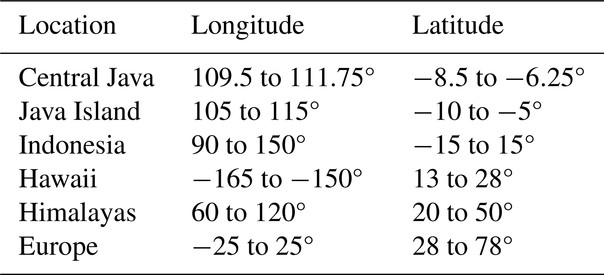
We demonstrate our approach at the following locations: Central Java, Java Island, the Indonesian Archipelago, the Hawaiian Islands, the Himalayan Mountain Range, and the European Plate. The corresponding geographic coordinates in decimal degrees are listed in Table 1.

The Earth2014 data (Hirt and Rexer, 2015) contain rock-equivalent topography that can be converted into topographic load by using the reference density and the gravitational acceleration in Table 2. For Central Java, we consider both a single-patch and multi-patch parameterization of the domain to show the capabilities of multi-patch isogeometric analysis when the data required for the simulation are only available for certain parts of Earth's surface. The results can be compared with the Mohorovičić depth data obtained using the inversion of receiver functions from the work of Amukti et al. (2019). A Mohorovičić depth map is available for the European Plate (Grad et al., 2009), which is also used to estimate model parameters in Sect. 5.2.

Table 1 Geographic coordinates of locations of interest.

5.1 Simulation of the lithospheric depression

In this subsection, we compare the results obtained from the simple Airy–Heiskanen model of local isostasy with the regional model of flexural isostasy by Vening-Meinesz to simulate the lithospheric depression due to topographic loading and buoyancy. Isogeometric analysis is used to solve the isostatic boundary value problem for the flexural model numerically. We choose the physical parameters in Table 2, which are assumed to be constant over the simulation domain. The mesh is subdivided into 16×16 elements, and a spline degree of (4,4) is chosen for the isogeometric spline space.

Table 2 Physical parameters for the numerical simulations.

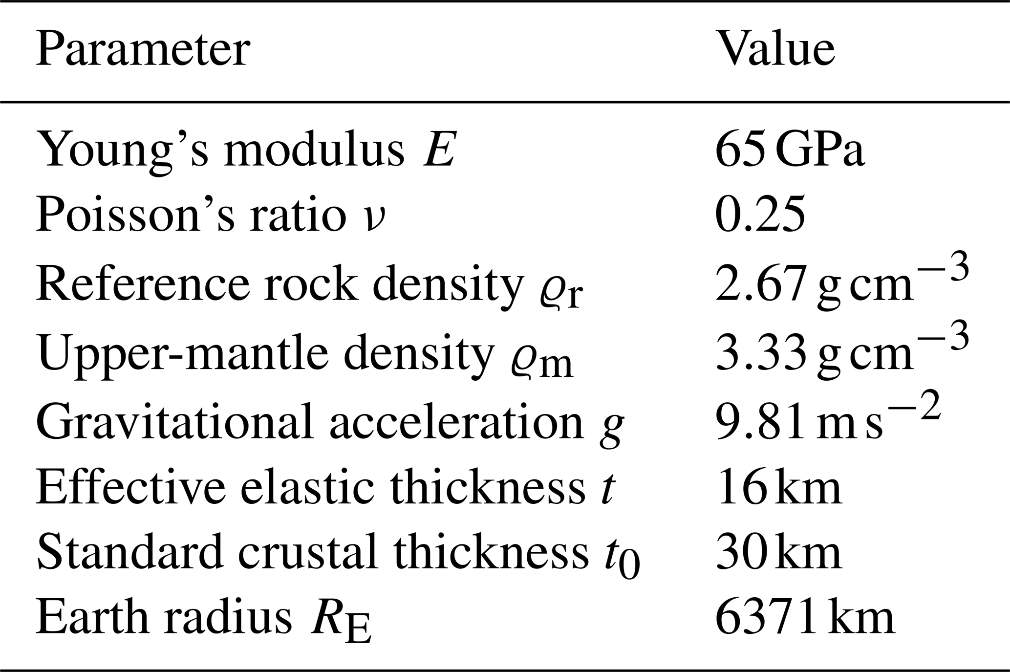
Figure 8a (left) shows a contour plot of the bedrock topography of Central Java. The corresponding topographic load, expressed through rock-equivalent topography, is shown in Fig. 8a (right), which also contains a multi-patch geometry of the domain of interest.

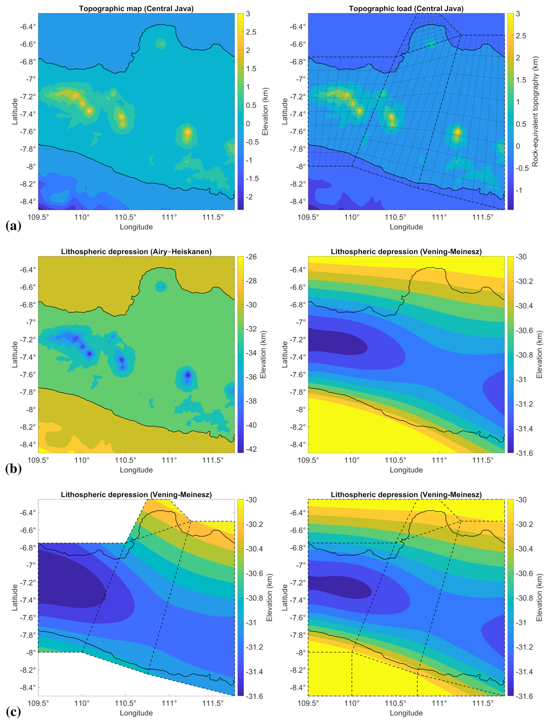
Figure 8 Numerical simulations of the lithosphere in Central Java. (a) Topographic map (left), corresponding load (right), and an example of a multi-patch geometry of Central Java (grid lines). (b) Lithospheric depression in Central Java according to the Airy–Heiskanen (left) and Vening-Meinesz (right) model. (c) Comparison between the partial (left) and the full (right) multi-patch parameterization of the domain.

The computed lithospheric depression for a single-patch domain is shown in Fig. 8b (right). Compared to the Airy–Heiskanen model in Fig. 8b (left) and the available depth data (Amukti et al., 2019, Fig. 6), the topographic loading in the Vening-Meinesz model is additionally compensated for by flexural rigidity. This leads to fewer local variations. High-frequency details are strongly attenuated, and the mid-surface only reaches a depth of less than 32 km as opposed to the Airy–Heiskanen model that predicts Mohorovičić depths of up to 42 km below mean sea level when using the same physical parameters.

The result of the multi-patch simulation is depicted in Fig. 8c (left). It differs from the single-patch result due to the missing data outside of the simulation domain that are replaced by Neumann boundary conditions. Augmenting the multi-patch domain with additional patches that cover the whole rectangular single-patch domain yields a result that is close to the single-patch solution (see Fig. 8c, right). Both solutions also appear to be continuously differentiable at the interfaces and require less computational effort and degrees of freedom than a classical approach using conforming C¹ finite elements or non-conforming discrete Kirchhoff elements, provided that multiple patches are used sparingly.

Numerical experiments for the other geographic locations have been done to observe the effect of different scales and varying load distributions. Large-scale simulations require more degrees of freedom to resolve tiny details of the solution. Uniform refinement of the mesh leads to a rapid increase in computational effort, which may not be necessary for regions that are already resolved to a sufficient accuracy. In order to reduce the computational effort by only adding degrees of freedom to regions that require more accuracy, we consider adaptive local refinement using hierarchical B-splines and a multi-level estimator with the maximum strategy (Garau and Vázquez, 2018). For the European Plate, we compare the results of using a uniform mesh with 16×16 elements and a hierarchical mesh arising from adaptive local refinement in Fig. 9b (right) and Fig. 9c, respectively.

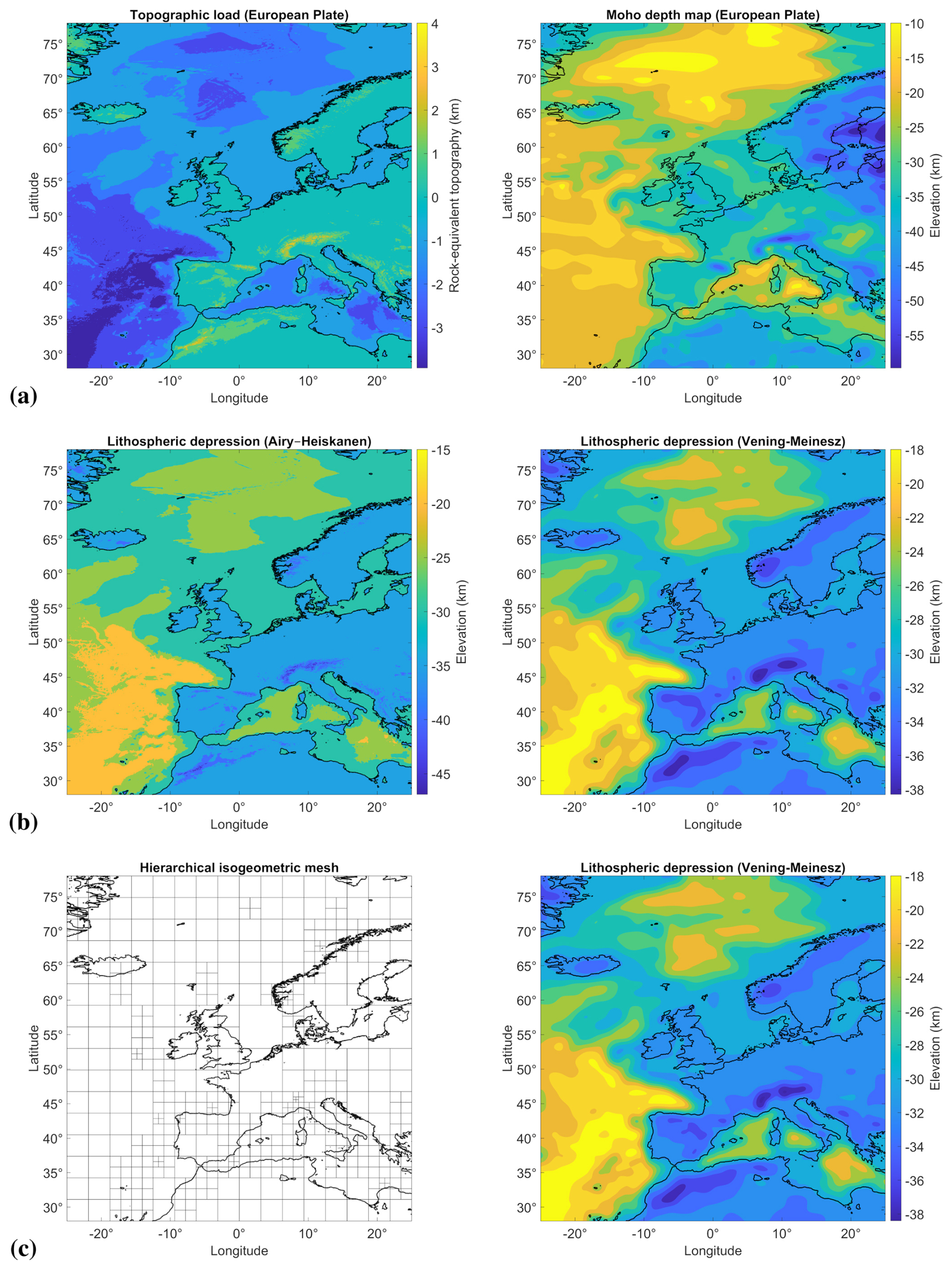
Figure 9 Numerical simulations of the lithosphere in Europe. (a) Topographic load (left) and Mohorovičić depth map (right) of Europe. (b) Lithospheric depression in Europe according to the Airy–Heiskanen (left) and Vening-Meinesz (right) model. (c) Adaptive local refinement of the isogeometric mesh in Europe (left) and corresponding lithospheric depression (right).

5.2 Parameter estimation from available data

The following parameters of the model have been estimated using the method in Sect. 4 and the available Mohorovičić depth map of Europe: effective elastic thickness of the lithosphere, rock density in the crust, and existing topographic load. The depth data stem from the work of Grad et al. (2009) and can be seen in Fig. 9a (right). A homogeneous effective elastic thickness of 16 km and a homogeneous reference density of 2.67 g cm⁻³ are assumed when they are not subject to estimation. These default values are furthermore used as initial values for the estimation process.

We use the Earth2014 data by Hirt and Rexer (2015) for the topographic load in Europe (see Fig. 9a, left). When topographic load is the sought parameter, the initial value for the corresponding rock-equivalent topography is set to 1 km everywhere. The lithospheric depression that results from the default values and the topographic data are depicted in Fig. 9b (right). These differ from the available Mohorovičić depth data due to simplified assumptions and missing information on position-dependent parameters of the model.

The estimated effective elastic thickness is mostly around 16 km (see Fig. 10a, left). There are particular spots scattered around the Mediterranean Sea and west of the British Isles that exhibit a slightly higher and lower thickness. A change in the effective elastic thickness of this magnitude does not significantly alter the resulting lithospheric depression; compare Fig. 10a (right) and Fig. 9b (right). Overall, the result is incompatible with the spatial distributions found in Pérez-Gussinyé and Watts (2005). According to Forsyth (1985), the flexural rigidity inferred from topographic loading is likely to be underestimated when there is significant internal loading due to subsurface variations, which has been disregarded in our simplified model.

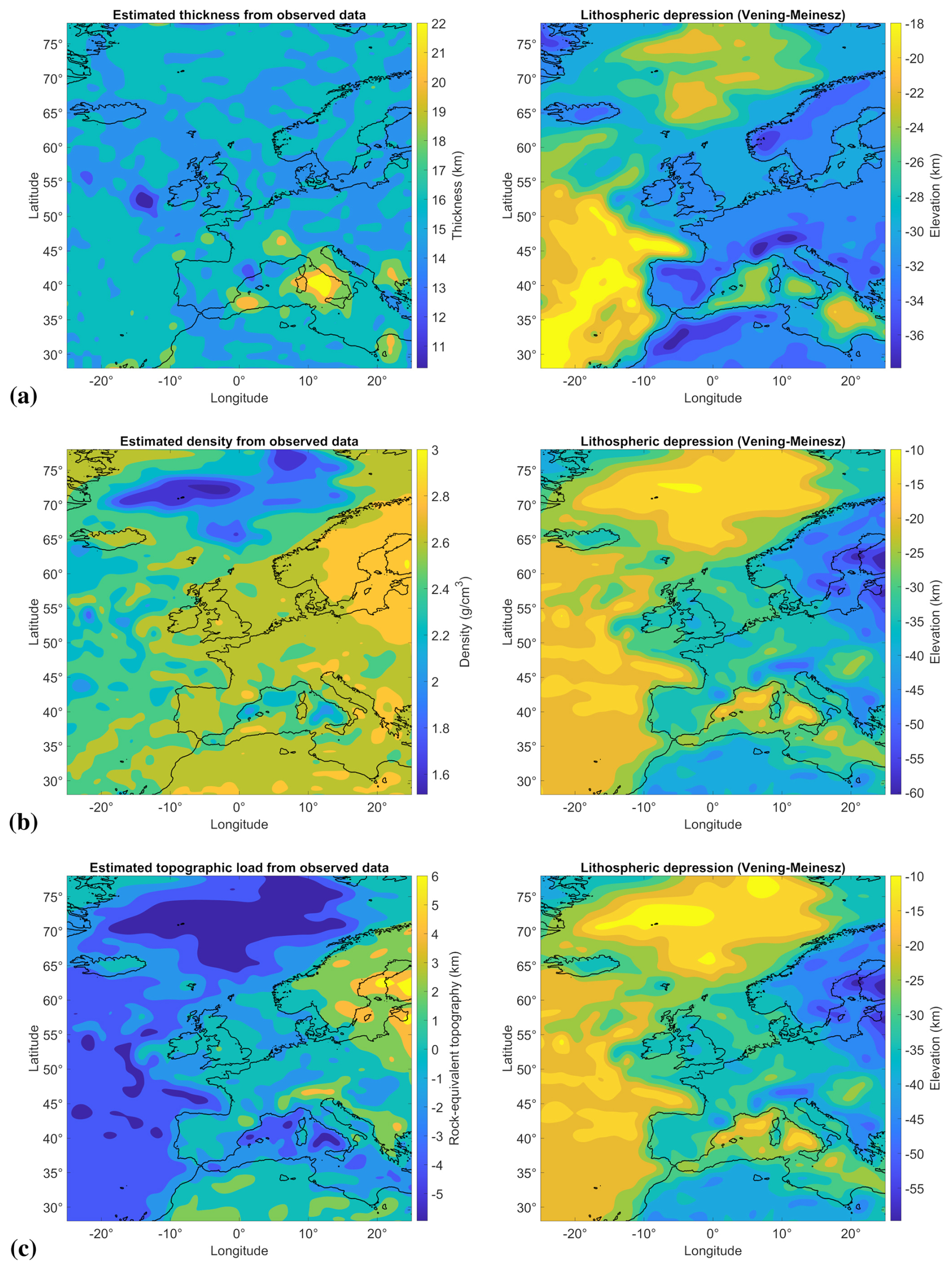
Figure 10 Parameter estimation of the effective elastic thickness, reference rock density, and topographic load in Europe. (a) Parameter estimation of the effective elastic thickness in Europe (left) and corresponding lithospheric depression (right). (b) Parameter estimation of the reference rock density in Europe (left) and corresponding lithospheric depression (right). (c) Parameter estimation of the topographic load in Europe (left) and corresponding lithospheric depression (right).

The parameter estimation predicts a higher reference density in the Baltic Shield and a lower reference density around oceans, especially in the Norwegian Sea (see Fig. 10b, left). The resulting lithospheric depression (Fig. 10b, right) is similar to the Mohorovičić depth map in Fig. 9a (right). A density distribution like the estimated one can explain the observed Mohorovičić depth data well.

The lithospheric depression that results from topographic load estimation is similar to the one that results from density estimation; compare Fig. 10b (right) and Fig. 10c (right). Since the effective elastic thickness and the rock density of the lithosphere are constant, the estimated topographic load seems to mimic the contours of the Mohorovičić depth map (see Fig. 10c, left).

5.3 Spherical model of the lithosphere

For the discretization of the variational problem in Sect. 2.4, we use a C¹ multi-patch parameterization arising from a quad sphere projection (see Fig. 11b). The parameterization is not analysis-suitable G¹ continuous. However, a similar one that is analysis-suitable can be constructed from it according to Kapl et al. (2018). The new parameterization will not necessarily represent the same geometry as before. Nevertheless, it can be used to obtain an analysis-suitable G¹ multi-patch parameterization of a surface that is close to a sphere.

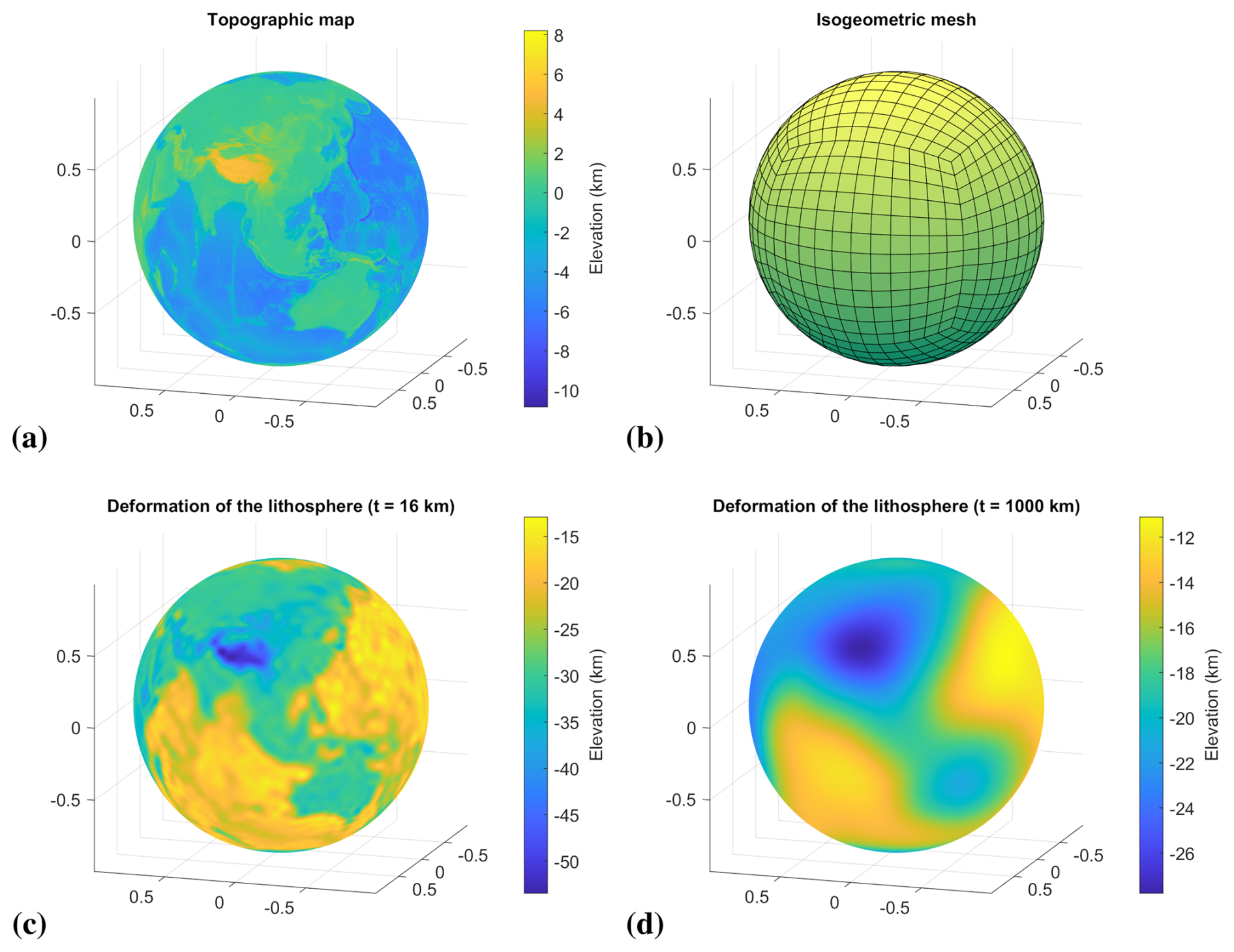
Figure 11 Numerical simulations of Earth's lithosphere modeled as a thin elastic spherical shell. (a) Global topographic map of the Earth. (b) Isogeometric mesh of the spherical domain. (c) Deformation of the lithosphere corresponding to an effective elastic thickness of 16 km. (d) Deformation of the lithosphere corresponding to an effective elastic thickness of 1000 km.

An effective elastic thickness of 16 and 1000 km is chosen for the lithosphere. The latter serves to demonstrate the effects of flexural rigidity on a spherical shell under internal pressure since the effects are negligible if the thickness is extremely small relative to the scale of the Earth. The Earth2014 data by Hirt and Rexer (2015) are mapped onto the sphere using a reverse geographic projection (see Fig. 11a). The resulting deformation of the lithosphere in isostatic equilibrium is shown in Fig. 11c and d, where elevation refers to the radial displacement relative to the reference sphere when a spherical Earth of constant radius is assumed. Note that the scale of the coordinate system is normalized to the radius of the Earth, which is specified in Table 2.

6 Conclusions

In this paper, we modeled Earth's lithosphere as a thin elastic shell and presented numerical methods of isogeometric analysis to simulate its deformation in isostatic equilibrium. Partial differential equations that involve higher-order derivatives and require a certain smoothness of the solutions can be discretized and solved without much effort and with fewer degrees of freedoms than standard finite-element methods using isogeometric analysis on a single patch. For more complex geometries that admit an analysis-suitable G¹ multi-patch parameterization, it is possible to construct multi-patch isogeometric spline spaces that preserve the global C¹ condition. Another feature of isogeometric analysis is its ability to represent curved domains exactly, which has been demonstrated by the simulation of a spherical shell, used to model the entire lithosphere of the Earth. Isogeometric analysis provides a versatile tool for numerically solving problems in geoscientific applications.

Aside from simulations of the lithospheric depression at selected geographic locations, we presented a method based on least-square estimation constrained by partial differential equations to identify parameters that are most plausible for the plate model when a ground truth is available. This has been applied to estimate the spatial distribution of the effective elastic thickness, the rock density, and the topographic load of the European Plate. Further improvements to the modeling approach have to be considered to obtain more reliable results since the computations were based on a fairly simple model of the lithosphere that does not take internal loading due to subsurface variations into account.

Appendix A: List of symbols

Symbol	Description
ℝk	Euclidean space of dimension k
${\mathit{e}}_{\mathrm{0}},\mathrm{\dots },{\mathit{e}}_k$	standard basis vectors in ℝk
ℬ	three-dimensional shell body
𝒜	reference surface (mid-surface)
X	particle in the body
ξ,ξ0	(initial) shell configuration
γ,γ0	(initial) mid-surface configuration
n,n0	(initial) unit normal vector field
${\mathit{\vartheta }}^{\mathrm{1}},{\mathit{\vartheta }}^{\mathrm{2}},{\mathit{\vartheta }}^{\mathrm{3}}$	local curvilinear coordinates ϑ
t	effective elastic shell thickness
V	shell potential energy
W	stored-energy density function
Fext,fext	(vertical) external body force
Gext,gext	(vertical) external surface force

Symbol	Description
fgrav,fbuoy	gravitational and buoyancy force
E	Saint Venant–Green material strain tensor
Em,em	(linearized) membrane strain
Eb,eb	(linearized) bending strain
Sm,sm	(linearized) membrane force
Sb,sb	(linearized) bending moment
K	elasticity tensor
E	Young's modulus
ν	Poisson's ratio
$D,\stackrel{\mathrm{̃}}{D}$	flexural rigidity (for a beam)
u	displacement field
v	variation of the displacement
w	vertical deflection field
v	variation of the vertical deflection
a	bilinear form for the stiffness matrix
b	bilinear form for the mass matrix
c	linear functional for gravitational load
ℓ	linear functional for external load
d,d0	(initial) mid-surface depth
t0	standard crustal thickness
h	topographic elevation
r	rock-equivalent topography
ϱ	density of overlying mass

Symbol	Description
ϱm	upper-mantle density
ϱr	reference rock density
g	gravitational acceleration
Bk,p	kth B-spline basis function of degree p
$N_{k,p}^{\mathit{\omega }}$	NURBS basis function with weight ω
${\mathit{N}}_{\mathit{\alpha }},{\mathit{N}}_{k,l}$	αth vector-valued NURBS basis function
${\mathcal{S}}_{d,r}^{\mathit{\omega }}(\mathbf{\Theta },\mathit{p})$	space of d-variate NURBS patches in ℝr
${\mathit{\vartheta }}_{\mathrm{0}},\mathrm{\dots },{\mathit{\vartheta }}_m$	spline knots in a knot sequence Θ
$p_{\mathrm{1}},\mathrm{\dots },p_d$	spline degrees in a tuple of degrees p
${\mathit{c}}_{\mathrm{0}},\mathrm{\dots },{\mathit{c}}_n$	control points of a NURBS patch in ℝr
${\mathit{\omega }}_{\mathrm{0}},\mathrm{\dots },{\mathit{\omega }}_n$	NURBS weights in a tuple of weights ω
ω	weight function
[a,b]	closed interval from a to b
(a,b)	open interval from a to b
[a,b)	left-closed and right-open interval from a to b
(a,b]	left-open and right-closed interval from a to b
$\mathrm{\Omega },\widehat{\mathrm{\Omega }}$	physical and parameter domain
$\mathcal{V},\widehat{\mathcal{V}}$	solution space on Ω and $\widehat{\mathrm{\Omega }}$
${\widehat{\mathcal{V}}}_{h,p}$	discrete solution space for ${\widehat{\mathit{u}}}_{h,p}$ and ${\widehat{\mathit{v}}}_{h,p}$
G	degrees of freedom for the geometry function
U,V	degrees of freedom for trial and test functions
A,L	coefficient matrix and right-hand side
C	constraint matrix for the C1 condition
Γ	patch interface
J	objective function
I	reduced cost functional
R	state equation operator
q	design variable (flexural parameter)
w	state variable (vertical deflection)
wd	observed data
p	crustal depth-to-height ratio
RE	Earth radius
C1	space of continuously differentiable functions
G1	space of geometric C1 functions
L2	Lebesgue space of square-integrable functions
H2	Hilbert–Sobolev space of order 2
$|\cdot |$	absolute value
$\Vert \cdot \Vert$	Euclidean norm
$\langle \cdot ,\cdot \rangle$	duality pairing
⋅	standard dot product
:	double tensor contraction
×	cross product
⊗	tensor product
[[⋅]]	interface jump
dA	area element
dS	length element
$\mathrm{d}x,\mathrm{d}y,\mathrm{d}z$	differential of coordinate functions $x,y,z$
$\frac{\mathrm{d}}{\mathrm{d}x}$, $\frac{{\mathrm{d}}^{\mathrm{2}}}{\mathrm{d}{x}^{\mathrm{2}}}$	first and second derivative operator
∂	boundary operator
∂1, ∂2	partial differential operators
δ	first variation operator
∇	gradient operator
∇2	Hessian operator
Δ	Laplace operator
𝒪	big O symbol

Symbol	Description
∈	element symbol
⊂	subset symbol
→	mapping symbol
∘	function composition
T	matrix transpose
|	restriction symbol