pyVPRM: a next-generation vegetation photosynthesis and respiration model for the post-MODIS era

The Vegetation Photosynthesis and Respiration Model (VPRM) is a well-established tool for estimating carbon exchange fluxes between the atmosphere and the biosphere. The gross primary production (GPP) and respiration (R_eco) of the ecosystem are modeled separately at high spatial and temporal resolution using the satellite-derived enhanced vegetation index (EVI) and land surface water index (LSWI), as well as meteorological variables for solar irradiance and surface temperature. The net ecosystem exchange (NEE) is calculated as the difference between the gross flux GPP and respiration. VPRM is widely used as a biospheric flux model in atmospheric transport modeling, most often on scales ranging from city to continent, but also in studies of biospheric carbon budgets and their changes with climate extremes. Historically, satellite-based surface reflectances from the 500 m resolution Moderate Resolution Imaging Spectroradiometer (MODIS) have been used to determine the EVI and LSWI. However, MODIS is reaching the end of its lifetime and will soon be decommissioned. Therefore, we present an updated version of VPRM, pyVPRM, which provides a software framework with a modular structure that can be used with various satellite products, land cover maps, meteorological data sources, and VPRM model parameterizations. Our tool naturally provides an interface to use satellite data from Sentinel-2, MODIS, and VIIRS, as well as global high-resolution land cover classification maps from the Copernicus Dynamic Land Cover Collection 3 and ESA WorldCover at 100 and 10 m resolution, respectively. Neither product is static; hence, dynamic changes of the land cover from year to year can be represented. Using Sentinel-2, ecosystem fluxes can be calculated at a resolution of up to 20 m, providing more accurate flux estimates in heterogeneous landscapes like croplands and making it possible to resolve small-scale vegetation patches common in urban areas. In contrast, VIIRS data are at the same resolution as MODIS and thus can provide continuity once MODIS is discontinued, requiring only minor adjustments to the VPRM data preprocessing. In addition, pyVPRM improves the data handling, for example, for snow-covered scenes. This paper presents the pyVPRM framework, discusses changes and improvements compared to previous VPRM implementations, and provides VPRM parameters for the European domain based on indices calculated from MODIS, Sentinel-2, and VIIRS using a new selection of eddy-covariance observations from 97 flux tower sites. Using pyVPRM and the new parameters, we observe significant improvements in the estimation of the European carbon budget. The results conform well with those from inversion studies.

1 Introduction

Carbon dioxide (CO₂) is the most important anthropogenically influenced greenhouse gas in the Earth's atmosphere and plays a decisive role in the carbon cycle. Carbon cycling occurs between the different compartments/reservoirs (i.e., atmosphere, oceans, and biosphere) of the Earth system on different timescales. The largest exchange flux of carbon is between the atmosphere and the terrestrial biosphere (Friedlingstein et al., 2023). This uptake flux is driven by the biosphere's photosynthesis (gross primary production, or GPP), i.e., the conversion of carbon dioxide, light, and water into sugar and oxygen. At the same time, carbon dioxide is released back to the atmosphere by respiration from plants and soil. The net vegetation flux into the atmosphere, i.e., the net ecosystem exchange (NEE), is given by the difference between the GPP and respiration. With a yearly global GPP of around 120 GtC, biospheric carbon dioxide fluxes are about an order of magnitude larger than anthropogenic emissions (with a yearly emission of 11.1 GtC in 2022; see Friedlingstein et al., 2023). Clearly, biospheric fluxes have an important impact on the time-dependent CO₂ concentrations in the atmosphere. Over longer timescales, GPP and respiration are nearly in balance, with a net carbon sink of around 3 GtC per year (Friedlingstein et al., 2023).

Terrestrial biosphere models (TBMs) are commonly used to simulate the carbon exchange between the biosphere and the atmosphere. They can be used to study the carbon budget of the terrestrial biosphere, as well as the impact of droughts and other climate extremes (Thompson et al., 2020; Stocker et al., 2019). Frequently, TBM outputs are also used as an input in atmospheric transport models, e.g., for the (inverse or top-down) estimation of carbon budgets from anthropogenic and natural sources from city to global scales (Bousquet et al., 1999; Sargent et al., 2018). Those top-down estimates of anthropogenic CO₂ emissions, informed by atmospheric concentration measurements, are expected to become an integral part of the global stocktakes required by international climate treaties (Maksyutov et al., 2019). They provide complementary information to the “bottom-up” methods, which combine activity data with emission factors to derive the budget (Choulga et al., 2021).

There are several TBMs that utilize remote-sensing data to locally estimate the plant and water dynamics (Nelson et al., 2024; Gerbig and Koch, 2021; Randerson et al., 1996; Running and Zhao, 2021). The Vegetation Photosynthesis and Respiration Model (VPRM) is a well-established light-use-efficiency TBM that estimates GPP, respiration, and, consequently, NEE from satellite-derived indices and meteorological drivers (Mahadevan et al., 2008). VPRM parameters are estimated using in situ measurements from eddy-covariance flux towers in different regions, for different years, and across different vegetation classes. Historically, VPRM has mainly been used with observations from the 500 m resolution Moderate Resolution Imaging Spectroradiometer (MODIS) instrument, installed on board the Terra and Aqua satellites¹, combined with the 1 km resolution SYNMAP land cover classification map (Jung et al., 2006).

Several modifications of the standard VPRM have been discussed in the literature. A common modification is a more sophisticated term for R_eco by, for example, including additional information on water stress (Gourdji et al., 2022) or adjusting the temperature response function (Sun et al., 2023). Other customized VPRM applications are the UrbanVPRM model for cities (Hardiman et al., 2017), the PolarVPRM for high-latitude ecosystems (Luus and Lin, 2015), a regional version for China (China-VPRM, Dayalu et al., 2018), approaches that incorporate information from solar-induced fluorescence (Commane et al., 2017), and a version to run online in the greenhouse gas module of the Weather Research and Forecasting (WRF) model (Ahmadov et al., 2009). All of these VPRM implementations rely on indices derived from MODIS.

The first MODIS sensor was launched in 1999, and since then the series of instruments have provided nearly a quarter-century time series of consistent data with high temporal resolution. Due to an onboard fuel shortage, MODIS will be decommissioned at the end of 2025, and hence alternative data sources are needed for VPRM.

In this paper, we present a new software package – pyVPRM (https://github.com/tglauch/pyVPRM, last access: 24 July 2025) – which adapts the VPRM to the post-MODIS era. It has an interface for new satellite datasets (Sentinel-2, VIIRS) and high-resolution land cover products (Copernicus Dynamic Land Cover Collection 3, Buchhorn et al., 2020; ESA WorldCover, Zanaga et al., 2022; and MapBiomas, Souza et al., 2020). Furthermore, it provides several improvements in terms of data handling, including the treatment of snow-covered scenes to improve stability and the use of the actual observation time when using time-aggregated products (like the 8 d MODIS products MOD09A1 (Vermote, 2021a) and MYD09A1 (Vermote, 2021b)) in the data smoothing process. In summary, those changes allow for a more accurate estimation of biospheric carbon dioxide fluxes, especially in regions with highly heterogeneous landscapes like cities or croplands. Thanks to its modular structure, pyVPRM can be easily extended by users to include further satellite products, land cover maps, meteorological datasets, and VPRM implementations.

This paper is structured as follows: in Sect. 2, we review the methodology of the standard VPRM model (Mahadevan et al., 2008). In Sect. 3, we discuss the improvements and changes in pyVPRM. In Sect. 4, we describe the estimation of the VPRM parameters for MODIS, VIIRS, and Sentinel-2 using a new selection of European flux tower sites. In Sect. 5, we discuss those parameters and their implications for European biospheric fluxes. In Sect. 6, we provide a discussion on the improvements, and we conclude in Sect. 7 with a summary and an outlook. A brief overview of the code structure is provided in Appendix A.

2 Review of the VPRM model

It should be noted that VPRM is not a centrally managed model, and implementations present throughout the literature differ significantly in their choices of vegetation classes and model equations. In this paper, we focus only on the original VPRM model implementation (Mahadevan et al., 2008) (called the vprm_base module in pyVPRM). For Mahadevan et al. (2008), eight vegetation classes are used: evergreen forest, deciduous forest, mixed forest, shrubland, savanna, cropland, grassland, and urban/non-vegetated.

All VPRM model implementations split the CO₂ flux between the terrestrial biosphere and atmosphere into two parts: gross primary production (GPP), driven by photosynthesis, and the sum of soil and plant respiration. In the standard VPRM (Mahadevan et al., 2008), the GPP is parameterized as

$$\begin{array}{}\text{(1)}& \mathrm{GPP}=\mathit{ϵ}\times {\displaystyle \frac{\mathrm{1}}{\mathrm{1}+\mathrm{PAR}/{\mathrm{PAR}}_{\mathrm{0}}}}\times \mathrm{PAR}\times \mathrm{EVI}.\end{array}$$

Here, EVI is the remote-sensing-based enhanced vegetation index (EVI), which is closely related to the productivity of vegetation (Huete et al., 2002). It is used as a measure of the fraction of absorbed photosynthetically active radiation (fAPAR, at wavelengths between around 400 and 700 nm) available for photosynthesis. EVI is usually based on measurements in the red, near-infrared, and blue bands, but a variant of this index can be calculated using only the red and infrared bands (see Sect. 3.1.1 for details). In contrast to other vegetation indices, like the normalized difference vegetation index (NDVI, Rouse et al., 1974), EVI is more sensitive to variations in canopy structure, including leaf area index (LAI), canopy type, and plant physiognomy (Huete et al., 2002).

The total amount of incoming photosynthetically active radiation can be approximated through the incoming shortwave (SW) radiation (direct and diffuse) at the surface using the relationship $\mathrm{PAR}\approx \mathrm{SW}/\mathrm{0.505}$ (Mahadevan et al., 2008). The term $\mathrm{1}/(\mathrm{1}+\mathrm{PAR}/{\mathrm{PAR}}_{\mathrm{0}}$) describes the saturation of the plants' photosynthetic activity. PAR₀ is the half-saturation value, one of the parameters fitted in the model for each vegetation class. Finally, ϵ is the light-use efficiency, which is the product of four terms with values between 0 and 1:

$$\begin{array}{}\text{(2)}& \mathit{ϵ}=\mathit{\lambda }\times T_{\mathrm{scale}}\times W_{\mathrm{scale}}\times P_{\mathrm{scale}}.\end{array}$$

Here, T_scale describes the temperature dependence of the photosynthesis, defined as

$$\begin{array}{}\text{(3)}& T_{\mathrm{scale}}={\displaystyle \frac{\left(T-T_{\min }\right)\left(T-T_{\max }\right)}{\left(T-T_{\min }\right)\left(T-T_{\max }\right)-{\left(T-T_{\mathrm{opt}}\right)}^{\mathrm{2}}}},\end{array}$$

with T_min, T_opt, and T_max referring to literature-derived values of the minimal, optimal, and maximal temperatures for photosynthesis for each vegetation class in degrees Celsius. At temperatures below T_min or above T_max, photosynthetic activity is set to 0. Usually, the temperature T is given by the 2 m temperature, which is available in most meteorological models.

The variable P_scale accounts for the effect of leaf age and is defined separately for the different vegetation types. For evergreen forests,

$$\begin{array}{}\text{(4)}& P_{\mathrm{scale}}=\mathrm{1};\end{array}$$

for grassland and savannas,

$$\begin{array}{}\text{(5)}& P_{\mathrm{scale}}=(\mathrm{1}+\mathrm{LSWI})/\mathrm{2};\end{array}$$

and for all other vegetation classes,

$$\begin{array}{}\text{(6)}& \begin{array}{rl}& P_{\mathrm{scale}}=\\ & \left\{\begin{array}{ll}\mathrm{1},& \mathrm{between}\mathrm{leaf}\mathrm{full}\mathrm{expansion}\mathrm{and}\mathrm{senescence}\left(\mathrm{EVI}>{\mathrm{TH}}_{\mathrm{leaf}\mathrm{full}\mathrm{expansion}}\right)\\ (\mathrm{1}+\mathrm{LSWI})/\mathrm{2},& \mathrm{during}\mathrm{bud}\mathrm{burst}\mathrm{to}\mathrm{leaf}\mathrm{full}\mathrm{expansion}\mathrm{and}\mathrm{during}\mathrm{senescence}\left(\mathrm{EVI}\le {\mathrm{TH}}_{\mathrm{leaf}\mathrm{full}\mathrm{expansion}}\right)\end{array}\right.\end{array}.\end{array}$$

Here, LSWI is the land surface water index, which captures the effects of water stress and leaf phenology and is derived using satellite data in the near and shortwave infrared (see Sect. 3.1.1 for details). The periods from bud burst to leaf full expansion and senescence are defined as those where the EVI is below a threshold of

$$\begin{array}{}\text{(7)}& {\mathrm{TH}}_{\mathrm{leaf}\mathrm{full}\mathrm{expansion}}={\mathrm{EVI}}_{\min }+\mathrm{0.55}\cdot \left({\mathrm{EVI}}_{\max }-{\mathrm{EVI}}_{\min }\right).\end{array}$$

Both the maximum and minimum EVI values (EVI_max and EVI_min) are calculated for each satellite pixel over an entire year.

The variable W_scale represents the canopy water content as a measure of the water stress. It is defined as

$$\begin{array}{}\text{(8)}& W_{\mathrm{scale}}=\left\{\begin{array}{ll}\frac{\mathrm{LSWI}-{\mathrm{LSWI}}_{\min }}{{\mathrm{LSWI}}_{\max }-{\mathrm{LSWI}}_{\min }},& \mathrm{grassland}\mathrm{and}\mathrm{savanna},\\ \frac{\mathrm{1}+\mathrm{LSWI}}{\mathrm{1}+{\mathrm{LSWI}}_{\max }},& \mathrm{all}\mathrm{other}\mathrm{classes}.\end{array}\right.\end{array}$$

The LSWI thresholds, LSWI_max and LSWI_min, are calculated as the pixel-wise maximum/minimum LSWI during the growing season (Eq. 7). Using this threshold ensures that the maximum LSWI lies within the growing season. This is important because LSWI is sensitive to snow periods.

Note that for grassland, we follow the parameterization of Matross et al. (2006), which takes into account that grasslands are xeric ecosystems. This represents a deviation from the work of Mahadevan et al. (2008) relevant for Eqs. (5) and (8).

Finally, λ is a fitting parameter that accounts for the quantum yield and also includes vegetation-class-specific (linear) corrections to the other parameters. For well-watered C₃ plants, the quantum yield is expected to be around 1/6 (Mahadevan et al., 2008).

The parameterization of ecosystem respiration, R_eco, is a simple linear function with two free parameters, α and β:

$$\begin{array}{}\text{(9)}& R_{\mathrm{eco}}=\mathit{\alpha }\times \max \left(T,T_{\mathrm{low}}\right)+\mathit{\beta }.\end{array}$$

When T<T_low, the temperature in Eq. (9) is set to T_low to maintain a minimal level of respiration, as the (winter) soil temperature is typically higher than the air temperature.

In summary, four free parameters α, β, PAR₀, and λ have to be fitted for each vegetation type.

3 The pyVPRM package

With pyVPRM, we provide a Python-based software package that can be used for a wide range of applications of the Vegetation Photosynthesis and Respiration Model (VPRM). It has a modular structure and can be used to combine different satellite data products, land cover maps, meteorology datasets, and VPRM model parameterizations. It provides all functions to fit VPRM parameters, produce biospheric fluxes, and generate input files for using VPRM online in mesoscale atmospheric transport models like the Weather Research and Forecasting model (WRF-GHG, Beck et al., 2012/WRF-Chem, Peckham, 2012) or the ICON-ART model (Schröter et al., 2018). An overview of the modular structure of pyVPRM is given in Fig. 1.

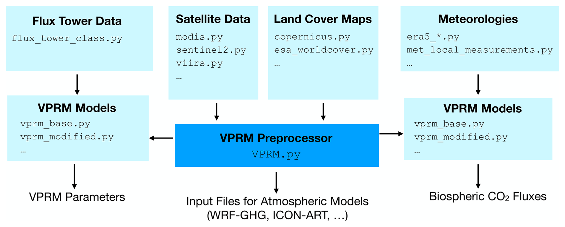
Figure 1 Modular structure of pyVPRM. Using different combinations of inputs, one can either calculate VPRM parameters, generate VPRM input files for atmospheric models, or calculate “offline” biospheric carbon dioxide fluxes. The type of module is shown in bold with the corresponding (exemplary) file name below. This is subject to changes and extensions in the further development of the model. The VPRM preprocessor is the central class that prepares the satellite images and land cover maps, as described in Sect. 3.1–3.3. More details are found in Appendix A.

3.1 Satellite data

In general, all multi-spectral satellites that have at least a near-infrared, a short wavelength infrared, and a red channel are suitable for constructing the indices required in the VPRM model. In addition, a blue band can be useful for the calculation of the enhanced vegetation index (EVI) but is not strictly necessary. While MODIS has been used historically, other satellite datasets are now available as well. Notably, Sentinel-2 (ESA, 2022) improves the VPRM spatial resolution from 500 m (MODIS (Vermote, 2021a, b; Vermote and Wolfe, 2021), VIIRS (Vermote et al., 2023a, b)) down to 20 m, which is especially useful for modeling ecosystem carbon dioxide fluxes in urban areas or in heterogeneous landscapes such as croplands and agricultural grasslands. The choice of satellite mission ultimately depends on the specific user requirements, e.g., the required spatial resolution, data availability, and satellite revisit time, especially when persistent cloud cover is an issue.

In its current implementation, pyVPRM provides an interface for satellite data products from MODIS, VIIRS, and Sentinel-2. Due to the modular structure, pyVPRM can be extended to other missions (e.g., Landsat) or fusion products of different satellite missions (e.g., Moreno-Martínez et al., 2020). VIIRS is of particular interest, as it is the drop-in replacement for MODIS after its discontinuation. A summary of the three satellite missions and the relevant mission specifications are given in Table 1. Evidently, there is a large overlap between the wavelength bands among the missions. Nevertheless, we fit a different set of VPRM parameters for each mission, accounting also for differences in the data processing, like the atmospheric correction.

Table 1 Overview of the relevant properties of the different satellite missions. The spatial resolution is given as the minimal resolution of all bands required for the VPRM calculations. In addition, the table names the MODIS (Vermote and Wolfe, 2021; Vermote, 2021a, b), VIIRS (Vermote et al., 2023a, b), and Sentinel-2 (ESA, 2022) data products used for the VPRM calculations in this paper. Note that for Sentinel-2, there is a slight difference in the bands between Sentinel-2A and Sentinel-2B. The values given here represent the bands of Sentinel-2A.

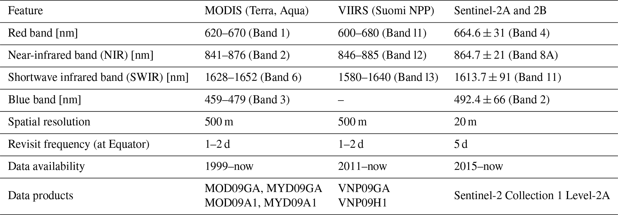
The MODIS sensor is placed on two research satellites – Aqua and Terra – with afternoon and morning orbits, respectively. Hence, combining data from the two satellite missions helps to mitigate sparse observations and improve the modeling of vegetation dynamics. This is especially useful in regions with high cloud coverage like the tropics. MODIS (Terra, Aqua) and VIIRS products are available as daily observations (MOD09GA, MYD09GA, VNP09GA) and as aggregated 8 d products (MOD09A1, MYD09A1, VNP09H1). The choice of optimal product depends on the expected vegetation dynamics and available computing resources. In this work, we use daily MODIS and VIIRS data, i.e., MOD09GA, MYD09GA, and VNP09GA.

3.1.1 Satellite indices

EVI is sensitive to the leaf area index, canopy type, and plant physiognomy. It is defined using the reflectances in red (ρ_Red), infrared (ρ_NIR), and blue (ρ_Blue) following Huete et al. (2002) as

$$\begin{array}{}\text{(10)}& \mathrm{EVI}=G\times {\displaystyle \frac{\left({\mathit{\rho }}_{\mathrm{NIR}}-{\mathit{\rho }}_{\mathrm{Red}}\right)}{\left({\mathit{\rho }}_{\mathrm{NIR}}+C_{\mathrm{1}}\times {\mathit{\rho }}_{\mathrm{Red}}-C_{\mathrm{2}}\times {\mathit{\rho }}_{\mathrm{Blue}}+L\right)}},\end{array}$$

where, in general, the free parameters G, C₁, C₂, and L depend on the satellite sensor. In our case, we use G=2.5, C₁=6, C₂=7.5, and L=1 (Huete et al., 2002) for both MODIS and Sentinel-2. While the detection of vegetation is governed by the red and infrared bands, the blue channel was added to account for the impact of atmospheric aerosols. It is, however, also possible to define an alternate enhanced vegetation index without a blue band (Jiang et al., 2008), EVI2, as

$$\begin{array}{}\text{(11)}& \mathrm{EVI}\mathrm{2}=G\times {\displaystyle \frac{\left({\mathit{\rho }}_{\mathrm{NIR}}-{\mathit{\rho }}_{\mathrm{Red}}\right)}{\left({\mathit{\rho }}_{\mathrm{NIR}}+C_{\mathrm{1}}\times {\mathit{\rho }}_{\mathrm{Red}}+L\right)}},\end{array}$$

with only three free parameters, i.e., G, C₁, and L. In our case, we use EVI2 for data from the VIIRS satellite, as no blue band is available. Here, the free parameters are set to G=2.5, C₁=2.4, and L=1 (Huete et al., 2002).

In addition to EVI, VPRM uses another remote-sensing-based index – the land surface water index (LSWI) – to estimate the vegetation and soil water content. LSWI requires a near-infrared and a shortwave infrared band and is calculated for all satellite missions following Gao (1995) as

$$\begin{array}{}\text{(12)}& \mathrm{LSWI}={\displaystyle \frac{{\mathit{\rho }}_{\mathrm{NIR}}-{\mathit{\rho }}_{\mathrm{SWIR}}}{{\mathit{\rho }}_{\mathrm{NIR}}+{\mathit{\rho }}_{\mathrm{SWIR}}}}.\end{array}$$

In pyVPRM, both EVI and LSWI are calculated within the VPRM preprocessor class (see Fig. 1) whenever a new satellite image is added to the instance (using the add_sat_img(.) function). The implementation of pyVPRM allows the user to adjust the free parameters in the function call or even add an entirely different implementation of satellite indices.

3.1.2 Data quality masking

Not every satellite observation is useful for the estimation of EVI and LSWI. Typical problems include cloudiness, shadows, and problems in the satellite retrieval. In order to get a reliable estimate of the time evolution of the two indices, pixels that have any of the previously mentioned problems are masked out from all further calculations using the data quality flags of the respective data products. Specifically, we use only pixels that have the highest-quality data in all bands, do not show any kind of cloud cover (also cirrus), and are free from cloud shadows. Periods with snow are treated differently; see Sect. 3.1.3. Details on the data quality flags for the satellite products discussed in this paper can be found in Table B1 (for MODIS), Table B2 (for VIIRS), and Table B3 (for Sentinel-2). In pyVPRM, the mask_bad_pixels(.), mask_bad_clouds(.), and mask_bad_snow(.) functions of the respective satellite image class are used.

3.1.3 Time smoothing

We expect both LSWI and EVI to be continuous functions over the year. Hence, in order to remove statistical noise, we derive daily indices through a temporal smoothing procedure (Mahadevan et al., 2008). In the first step, all the available satellite scenes for at least a year are loaded and combined into a data cube with two spatial dimensions and a time dimension. Subsequently, the array of observations in each pixel is smoothed using a lowess (LOcally WEighted Scatterplot Smoothing) function (Cleveland, 1979) (using the lowess(.) function of the VPRM preprocessor). The smoothing takes into account the specific observation time of each scene, even if 8 d products (like MOD09A1) are being used. Finally, the fitted lowess function is evaluated for each day of the year, producing a data cube storing daily EVI and LSWI for each pixel. It is good practice to include additional satellite scenes before the beginning and after the end of the year of interest to avoid boundary effects.

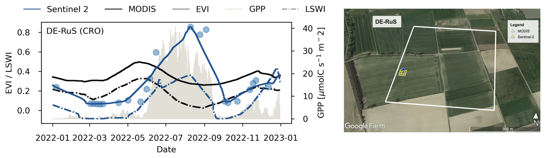
Figure 2 Left panel: comparison of the hourly GPP at the cropland flux tower site Selhausen Juelich (DE-RuS; 50.8659° N, 6.4471° E) with the satellite indices (EVI, LSWI) for Sentinel-2 and MODIS over the year 2022. GPP (in light gray) is based on the ICOS daytime partitioning method. The solid and dash-dotted lines show the lowess-smoothed LSWI and EVI, respectively. Values from MODIS are shown in black, while values for Sentinel-2 are shown in blue. The blue points show the unfiltered EVI measurements for the case of Sentinel-2. Right panel: satellite image of the site with the relevant MODIS (white) and Sentinel-2 (yellow) pixels overlaid. The position of the flux tower is shown with a blue pin. Map data © Google Earth 2024.

While the lowess function is fairly stable against noise, instabilities may arise if the vegetation is covered by snow for several months of the year (especially at high latitudes). Hence, instead of masking out every observation with detected snow cover, as we do for clouds and other low-quality observations, during snow-covered periods, we set the EVI and LSWI to the minimum value observed outside of the snow-covered period. This stabilizes the numerical fit and does not impact the estimated carbon fluxes, as the temperature during snow-covered periods is usually below 0° C, resulting in negligible GPP (see Eq. 3). The respiration, on the other hand, is independent of the satellite indices.

Figure 2 shows an example of the lowess-filtered values for EVI and LSWI from MODIS and Sentinel-2 at the German cropland flux tower site Selhausen Juelich (DE-RuS; 50.8659° N, 6.4471° E) in 2022. For comparison, hourly measured GPP is shown in the background. On average, the crosswind integrated distance, which contributes 90% of the flux measurement, is around 85 m at the eddy-covariance site DE-RuS (ICOS RI et al., 2023). A 2D map of the footprint is shown in Fig. 2b of Paulus et al. (2024). Evidently, the disagreement of the MODIS EVI curve with the measured GPP is a direct result of the limited spatial resolution of MODIS in such a heterogeneous landscape. In fact, the observed seasonal cycle of the satellite indices is a superposition of the seasonal cycles of the fields contained within the MODIS pixel (white). The field containing the flux tower itself was growing potatoes in 2022, which are only planted in April, take time to grow, and last until fall. The eastern and southeastern neighboring fields, in contrast, had winter wheat, which was sown the fall before, starts photosynthesis early, and is typically harvested around July (Marius Schmidt, personal communication, 2025). In contrast, the Sentinel-2 indices more closely follow the seasonal cycle of the GPP measurements. Uncertainties in Sentinel-2 arise mainly through the limited revisit frequency. While MODIS provides one image every 1–2 d under clear-sky conditions, Sentinel-2 takes only one image every ∼5 d. Hence, in time periods with frequent cloud coverage, observations can become sparse. The resulting interpolation errors are largest in periods of strong leaf phenological change.

We have exemplarily studied the impact of the revisit time for three flux tower sites with very homogeneous landscapes on the spatial scale of a MODIS pixel; see Fig. 3. For MODIS, we have used the daily Terra and Aqua observations (MOD09GA, Vermote and Wolfe, 2021/MYD09GA, Vermote, 2021a), and for Sentinel-2, Collection 1 Level-2A data from Sentinel-2A and 2B (ESA, 2022). The EVI curves for both satellites show a similar behavior. Small differences between the absolute EVI values are expected due to differences in the observation channels and resolutions. While Sentinel-2 curves show a little bit more instability, this is a minor effect on absolute scales. In general, we expect the instability of the smoothing to increase for regions with very frequent cloud coverage or long times without daylight (as in northern Scandinavia).

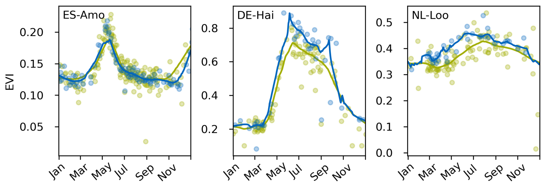
Figure 3 Development of the EVI for three test sites with different vegetation types in 2022: ES-Amo (shrubland), DE-Hai (deciduous forest), and NL-Loo (evergreen forest). Blue and green lines show the lowess-smoothed curves for Sentinel-2 and MODIS, respectively. The dots in the background show the cloud- and snow-filtered satellite observations.

3.2 Land cover classification

The standard VPRM model (Mahadevan et al., 2008), as described in Sect. 2, is fitted with four independent parameters for each vegetation class. In addition to remote sensing data, the estimation of terrestrial carbon fluxes with VPRM therefore requires a land cover classification map that covers the entire area of interest. In general, pyVPRM can be used with any kind of land cover product and vegetation classification. By default, the package provides interfaces for the global 100 m Copernicus Dynamic Land Cover Collection 3 (Buchhorn et al., 2020) and the global 10 m ESA WorldCover (Zanaga et al., 2022) product. Neither product is static in that they provide different maps for different years to account for land use changes.

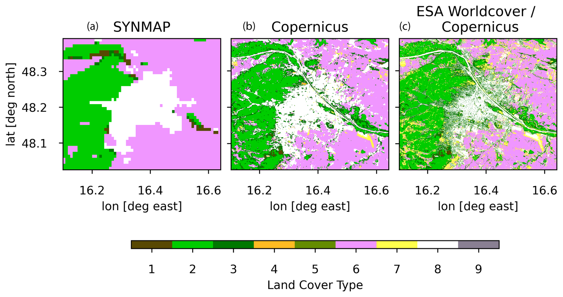
Figure 4 The region around Vienna for three different land cover classification products: SYNMAP (a), the 100 m product of the Copernicus Dynamic Land Cover Collection 3 (b), and a hybrid between ESA WorldCover and the Copernicus Dynamic Land Cover Collection 3 (c). Different colors (numbers) represent the different vegetation classes in our VPRM model for Europe: evergreen (1), deciduous forest (2), mixed forest (3), shrubland (4), cropland (6), grassland (7), non-vegetated area (8), and wetland (9). The class savanna (5) is not used in this implementation but remains in the numbered list for legacy reasons.

In addition, both land cover products do not provide a dedicated savanna class. We therefore drop it, which is reasonable for most parts of the mid-latitudes. In regions where this vegetation class is needed, it is advisable to use a dedicated land cover product and VPRM parameters. On the contrary, we have decided to add a new class for wetland. This is motivated by the larger amount of available flux tower measurements (cf. Fig. 6).

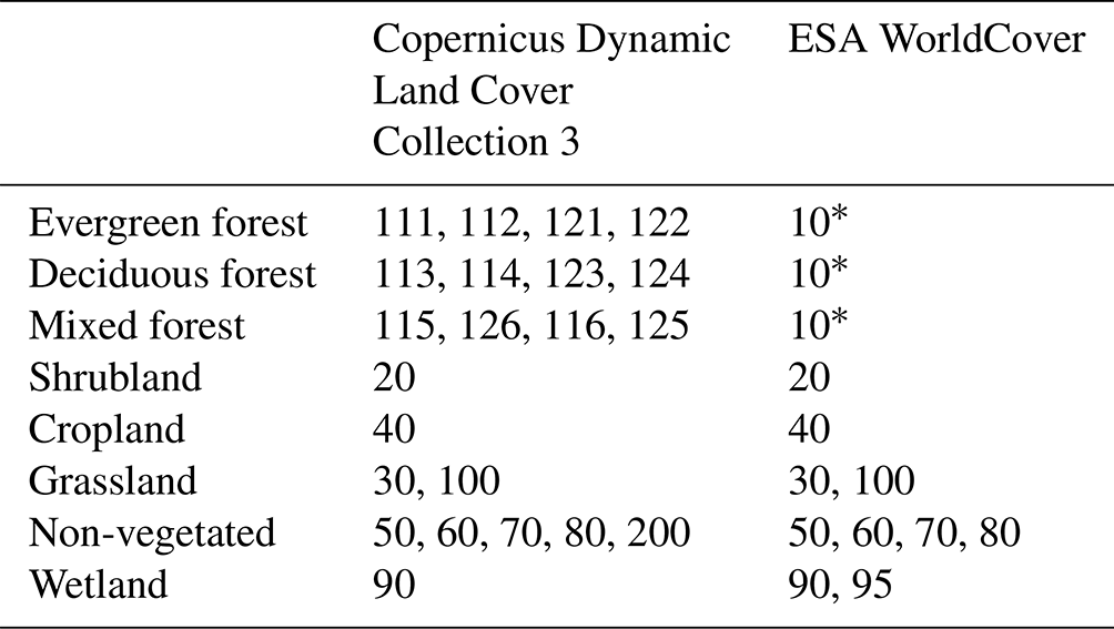
Table 2 shows the mapping between the land cover types for the two products and the eight VPRM classes used in this paper. Note that ESA WorldCover has only one forest class and, therefore, contains no information on the forest type. Hence, it is rational to generate a hybrid product that uses ESA WorldCover as a baseline but replaces the forest subclass information with that of the (lower-resolution) Copernicus Dynamic Land Cover Collection 3 (Buchhorn et al., 2020). A sequence of land cover maps with increasing resolution is shown for a region around Vienna in Fig. 4. Note that while SYNMAP (Jung et al., 2006) does not resolve much of the structure inside the built-up urban area, the Copernicus Dynamic Land Cover Collection 3 (Buchhorn et al., 2020) product and especially the hybrid product can resolve vegetated areas within the built-up area and heterogeneity within the forested area to the west of the city and the surrounding croplands.

Table 2 Mapping from land cover classifications in the Copernicus Dynamic Land Cover Collection 3 (Buchhorn et al., 2020) and ESA WorldCover (Zanaga et al., 2022) to the eight VPRM classes used in this paper. The numbers represent the internal land cover codes of the two data products. Note (^*) that ESA WorldCover has only one forest class. Hence, it is advised to use a hybrid of the two products in this table, using the forest-type classification of the 100 m products of the Copernicus Dynamic Land Cover Collection 3. pyVPRM uses YAML configuration files to define the mapping and auxiliary data for the vegetation classes.

In many cases, the land cover maps will not have the same coordinate reference system and resolution as the satellite data products. Hence, the land cover map needs to be regridded to match the satellite data. pyVPRM uses the xESMF package (Zhuang et al., 2023), which is based on the Earth System Modeling Framework (ESMF) (Hill et al., 2004). xESMF supports general curvilinear grids and different regridding algorithms, most importantly bilinear and conservative, in order to preserve total quantities. Using conservative regridding, the add_land_cover_map(.) function of pyVPRM's VPRM preprocessor calculates the fraction of each land cover class from the input (land cover) grid for each pixel in the destination (satellite) grid. The result is a 2D vegetation fraction map for each vegetation class with the same spatial extent and on the same grid as the satellite scenes.

3.3 VPRM data preparation and calculation of carbon fluxes

In order to generate the VPRM fluxes for a given region, we use Eqs. (1) and (9) in matrix form. This requires the meteorological data (e.g., temperature and solar irradiance) and the land cover information to be regridded onto the native satellite grid using the xESMF package; see Sect. 3.2. With all the data on the same grid, the net ecosystem exchange (or GPP and respiration) for each land cover type is calculated by matrix multiplication (using the make_vprm_predictions(.) function of the VPRM model class). Summing up all land cover types with their respective fractional weight, F_v, gives the total flux per pixel, i.e.,

$$\begin{array}{}\text{(13)}& \begin{array}{rl}{\mathrm{NEE}}_{\mathrm{2}\mathrm{D}}& =\sum _{\begin{array}{c}\mathrm{v}\in \\ \mathrm{veg}\mathrm{classes}\end{array}}{F}_{\mathrm{v}}\times \left[-\left({\mathit{\lambda }}_{\mathrm{v}}\times T_{\mathrm{scale},\mathrm{v}}\times W_{\mathrm{scale}}\times P_{\mathrm{scale},\mathrm{v}}\right)\right.\\ & \times {\displaystyle \frac{\mathrm{1}}{\mathrm{1}+\mathrm{PAR}/{\mathrm{PAR}}_{\mathrm{0},\mathrm{v}}}}\times \mathrm{PAR}\times \mathrm{EVI}+{\mathit{\alpha }}_{\mathrm{v}}\\ & \left.\times \max \left(T,T_{\mathrm{low},\mathrm{v}}\right)+{\mathit{\beta }}_{\mathrm{v}}\right].\end{array}\end{array}$$

3.4 VPRM preprocessor for online flux calculation in mesoscale atmospheric transport models

Complementary to the direct calculation of carbon fluxes, pyVPRM can also be used as a preprocessor to generate input files for online flux calculation within mesoscale atmospheric models, such as the greenhouse gas module of the Weather Research and Forecasting (WRF-GHG/WRF-Chem) model or ICON-ART. In this case, the fluxes are calculated using the 2 m temperature and shortwave radiation at the surface calculated within the atmospheric model. The procedure for the generation of the input files is similar to the procedure described in Sect. 3.3. The difference is that, instead of using Eq. (13) to calculate the CO₂ fluxes, the EVI and LSWI fields as well as the land cover map are regridded to match the input format of the atmospheric model. Overall, the VPRM preprocessor needs to create seven files: two containing the daily EVI and LSWI for each vegetation class, four with the annual minimum and maximum EVI and LSWI for each vegetation class, and one with the pixel-wise fraction of each vegetation class. In pyVPRM, the output files can be directly written from a VPRM preprocessor instance using the to_wrf_output(.) method. Figure 5 shows an example of the vegetation fractions for Europe using the Copernicus Dynamic Land Cover Collection 3 (Buchhorn et al., 2020) as input.

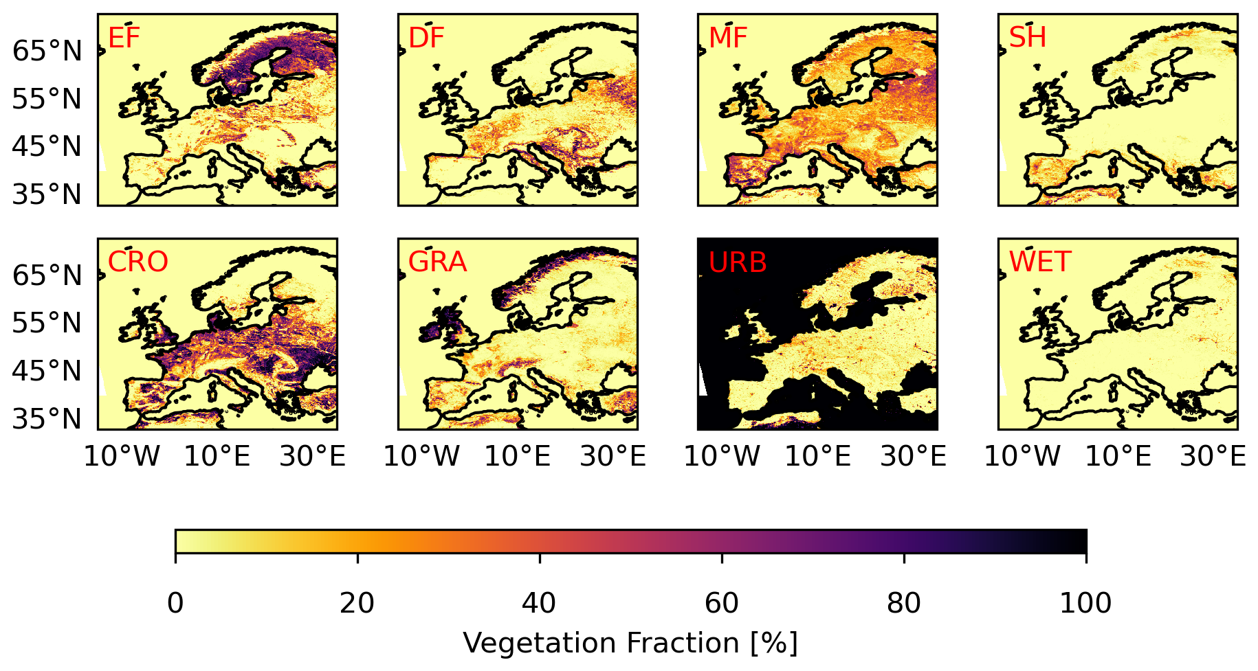
Figure 5 Vegetation fractions of the eight land cover classes used in our VPRM model, based on the Copernicus Dynamic Land Cover Collection 3. The data are regridded on a 0.25°×0.25° regular grid. This is a typical example of a vegetation fraction map that can also be used in mesoscale atmospheric models like WRF-GHG/WRF-Chem or ICON-ART. The abbreviations are evergreen forest (EF), deciduous forest (DF), mixed forest (MF), shrubland (SH), cropland (CRO), grassland (GRA), non-vegetated (URB), and wetland (WET). Not shown here are the other files generated by the pyVPRM preprocessor, i.e., the EVI and LSWI maps.

4 Estimating VPRM parameters for Sentinel-2, MODIS, and VIIRS

The full equation of the VPRM model, Eq. (13), contains four free parameters for each vegetation class: the quantum efficiency λ, the half saturation value of the photosynthetic activity PAR₀, and two parameters, α and β, describing a linear respiration model with temperature. Those parameters are required to calculate the carbon fluxes, whether VPRM is used offline or within the weather prediction/tracer transport model. To estimate those parameters, in situ CO₂ flux measurements from eddy-covariance towers are used. We show here an example of the fitting procedure for the European domain and provide an updated VPRM parameter set for Sentinel-2, MODIS, and VIIRS.

4.1 Flux tower selection

Several data collections provide harmonized eddy-covariance flux tower measurements for a collection of measurement sites. For example, the FLUXNET2015 data collection (Pastorello et al., 2020) provides global data for a total of 212 sites, but currently only up to the year 2015. On a continental level, AmeriFlux provides data for North and South America, the ICOS Carbon Portal (ICOS RI et al., 2023) provides data for Europe, and OzFlux provides data for Australia and New Zealand.

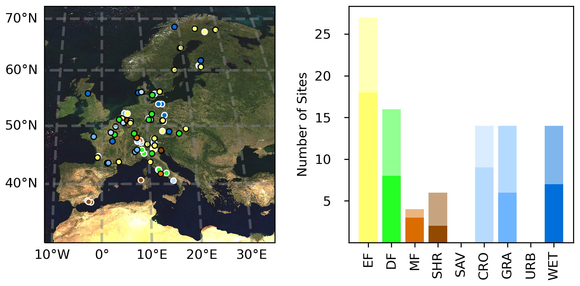
Figure 6 Left panel: the flux tower sites used to estimate the VPRM parameters. Circles with black and white contours indicate data that were used from the ICOS or FLUXNET data collection, respectively. Different colors show the different vegetation types with the number of sites shown in the histogram on the right. Brighter bars show the number of ICOS and FLUXNET stations with available data during the period covered by MODIS. Darker bars show the number of stations available since the launch of Sentinel-2. Abbreviations are as follows: EF – evergreen forest, DF – deciduous forest, MF – mixed forest, SHR – shrubland, CRO – cropland, GRA – grassland, WET – wetland, SAV – savanna. Background satellite image created using MODIS data.

For our European application, we combine data from FLUXNET and ICOS covering the period between 2002 and 2022. An overview of the locations and ecosystem types of the various stations is given in Fig. 6. For the fit of the Sentinel-2 parameters, only sites with data after 2015 can be used. To be consistent with previous VPRM versions (Gerbig and Koch, 2021), we use only 1 year of flux tower data per site. The year is selected as the year within the data acquisition period of the respective satellite with the maximum amount of available flux tower data. Overall, we use 97 sites for MODIS, 52 sites for Sentinel-2, and 68 sites for VIIRS. An overview of the stations used for parameter estimation is shown in Sect. D for each satellite mission.

All flux towers use the eddy-covariance technique, which determines vertical fluxes from turbulence-resolving (i.e., sub-second) measurements of the vertical wind component and the quantity of interest – in our case, CO₂ (Baldocchi et al., 2001; Swinbank, 1951). They measure a weighted average of fluxes in the upwind direction. The spatial area from which fluxes contribute to the measurement is called the footprint, and this depends strongly on the height above canopy of the flux tower itself, as well as other aerodynamic quantities such as the surface roughness (Chen et al., 2009; Schmid, 1994). Optimally, the flux tower should be surrounded by a sufficiently homogeneous landscape to be representative for a specific land cover class. This is, however, not always the case. For some sites, the measurement might see signals from different land cover types at different times (Järvi et al., 2012). Other sites might be located in a satellite pixel that overlaps with different land covers; see Fig. 2. For this reason, we visually inspect all sites using Google Earth and remove those that are extremely heterogeneous on the spatial scale of the satellite resolution.

4.2 Spatial smoothing

Spatial smoothing is a way to account for footprints that exceed the size of a single satellite pixel. In previous VPRM versions (Mahadevan et al., 2008), the EVI and LSWI of the nine MODIS pixels surrounding the tower location were averaged for comparison with the flux tower data. This means averaging over a region of around 1.5×1.5 km². In many cases, especially in Europe, the averaging is therefore done over heterogeneous land cover types, leading to inconsistencies between measured and modeled fluxes; see Fig. 10.

We mitigate this problem by dropping the spatial smoothing for MODIS and VIIRS (with 500 m resolution), i.e., we use only the pixel in which the tower is located. For Sentinel-2, with a pixel size of 20 m, we use a 3×3 pixel (60 m × 60 m) spatial smoothing centered at the tower location.

In general, pyVPRM also provides the option of using arbitrary weighting kernels in the smearing(.) function of the VPRM preprocessor to better match the satellite observation to flux tower footprint models.

4.3 Fitting VPRM parameters

For the fit, we choose only the highest-quality data points, thus removing low turbulence conditions with bad flux measurements (i.e., only using data where “NEE_VUT_REF_QC” is 0). Further, we ensure that the data are distributed uniformly over the year and the time of the day. To do that, we group the data in two dimensions by week of the year and time of the day in 3-hour time steps. Subsequently, we randomly sample three measurements from each group. This leads to a selection of 𝒪(10³) data points with uniform distribution over the year for each tower. The selected data are fitted using a two-step mean-squared-error fitting. In the first step, the respiration parameters are fitted for nighttime data only, thus naturally removing the light-dependent photosynthesis. In the second step, NEE is fitted using the best-fit parameters of the first step for the respiration parameters. This fitting procedure hence does not require a partitioning of the measured NEE into GPP and respiration but rather uses the flux measurements directly. This avoids typical assumptions and uncertainties that arise when partitioning the carbon fluxes from eddy-covariance towers (Wutzler et al., 2018). In pyVPRM, each VPRM model class has a function fit_vprm_data(.) that performs the fit.

5 Results

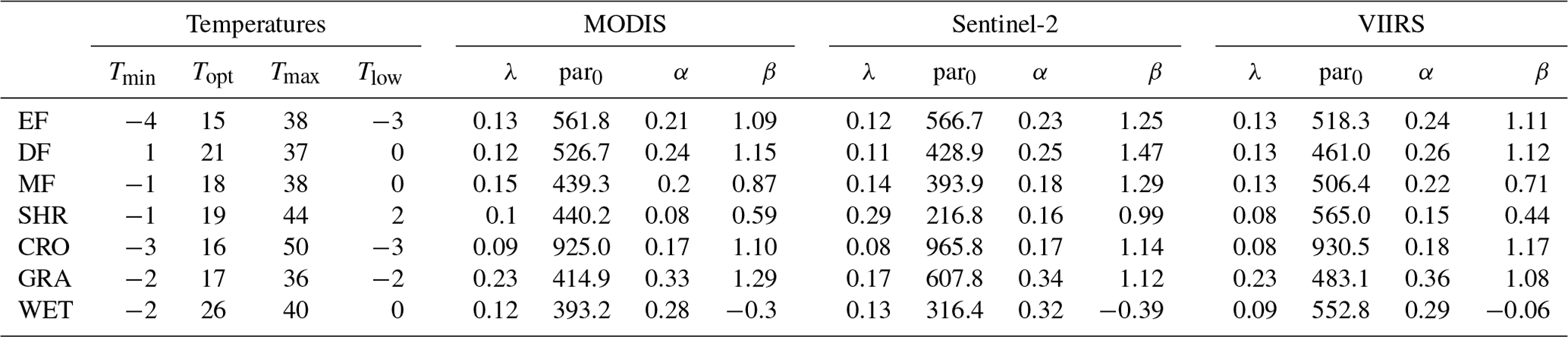
VPRM parameters for the different satellite missions (MODIS, VIIRS, Sentinel-2) for the European domain are shown in Table 3. We observe that, although the wavelength bands of MODIS and Sentinel-2 largely overlap, there are some differences between the parameters for the two products. This could be related to slight differences in the satellite bands and data collection or in the different spatiotemporal resolutions of the observations. This question will be investigated in further studies. The parameters for VIIRS are calculated using EVI2 (without the blue band) and hence are not expected to be directly comparable.

Table 3 Overview of the VPRM parameter sets for MODIS, Sentinel-2, and VIIRS and the different ecosystems. Abbreviations are as follows: EF – evergreen forest, DF – deciduous forest, MF – mixed forest, SHR – shrubland, CRO – cropland, GRA – grassland, WET – wetland. The parameters of Gerbig (2024) can be found in Table C1 for comparison.

In order to evaluate how the high resolution of Sentinel-2 can improve flux estimates, we have studied some of the (heterogeneous) cropland flux sites in more detail. In Fig. 7, the monthly average diurnal cycle is shown for the Selhausen Juelich site (DE-RuS; 50.8659° N, 6.4471° E). Evidently, the monthly median diurnal cycle of Sentinel-2 matches the observation much better than the one from MODIS in most months. This is a direct consequence of the different seasonal cycles of the EVI, as shown in Fig. 2. While the higher resolution of the Sentinel-2 images allows the growing periods of the specific field to be resolved, MODIS is averaging over several fields, resulting in a superposition of their seasonal cycles. This results in predicted fluxes in April and May that are much larger than what is observed at the site. Overall, the mean-squared deviation from the measurement reduces from 43.9 (MODIS) to 7.1 (Sentinel-2). Similar effects can be observed for many cropland sites, which is especially problematic in Europe, where 38 % of the land surface is covered with cropland. Figure 8 gives an overview of the mean-squared deviation from the measurement for the cropland sites with data availability during the Sentinel-2 mission. For comparison, we also show similar results for evergreen forest sites, which are usually pretty homogeneous (the same plot for deciduous and mixed forest is shown in the Appendix, Fig. G1). As expected, the majority of cropland sites show a significant reduction in the mean-square deviation, while there is no trend for evergreen forests (as for the other forest classes). The full diurnal cycles of all cropland sites in Fig. 8 are shown in Appendix E. Our findings are in line with a recent study of Bazzi et al. (2024) that found that using Sentinel-2 data significantly improves the simulation of cropland carbon dioxide fluxes in Europe.

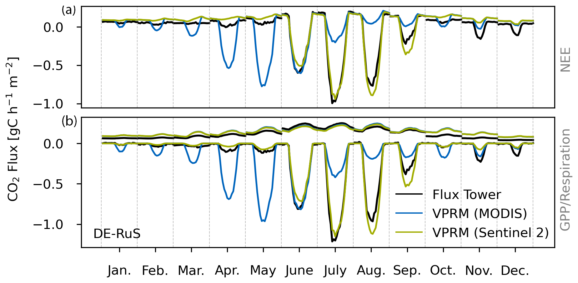
Figure 7 The mean diurnal cycle for each month at the cropland site Selhausen Juelich (DE-RuS, 50.8659° N; 6.4471° E) in 2022. The median tower measurements for each hour of the day are shown as black lines. Colored solid lines indicate the results from the VPRM model using indices from Sentinel-2 (green) and MODIS (blue). In the top panel, NEE is shown, and in the bottom panel, GPP (negative values, carbon uptake) and respiration (positive values, carbon release) are shown. The flux partitioning is based on the nighttime partitioning method with a variable u^* threshold (Reichstein et al., 2005).

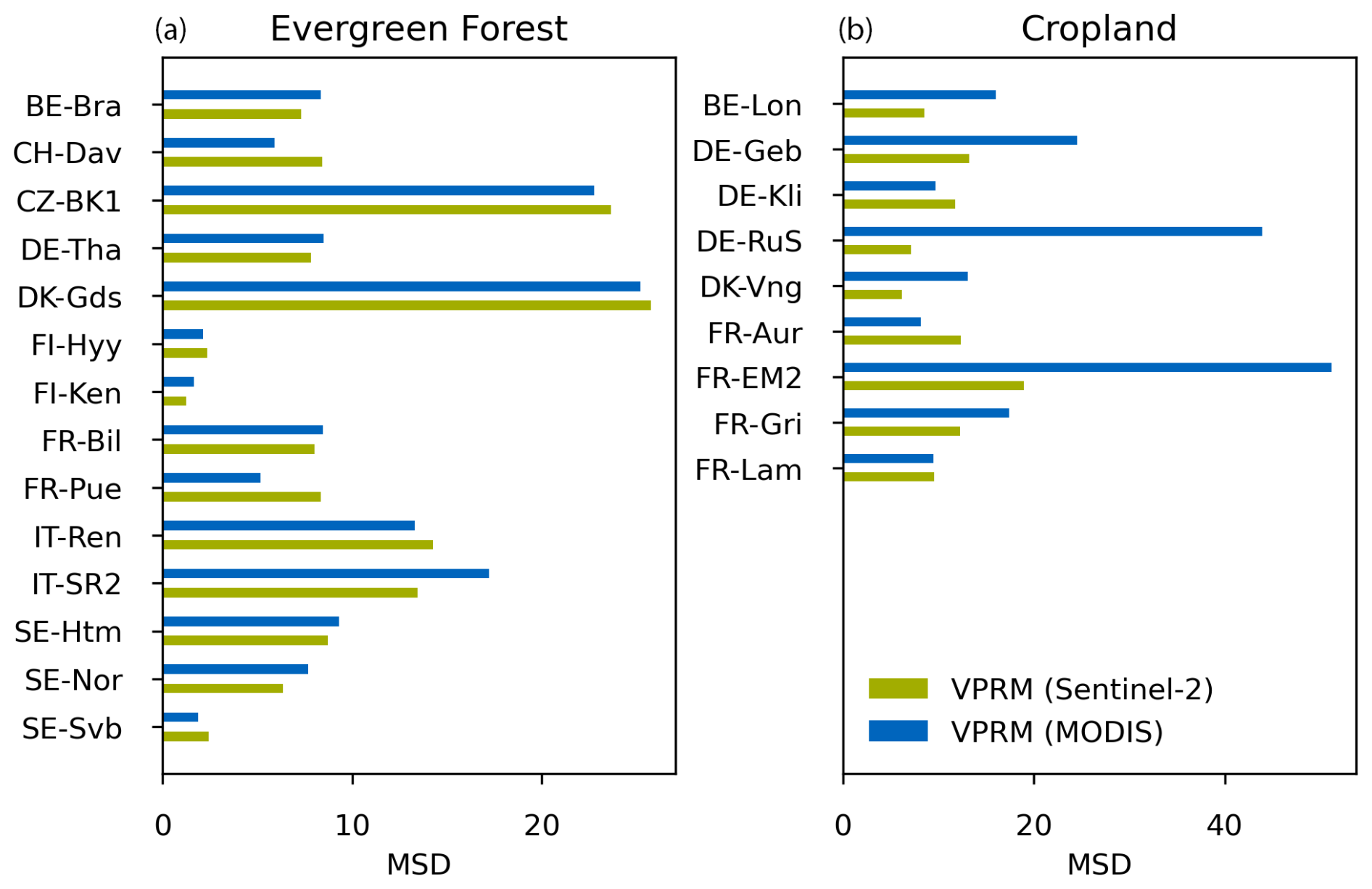
Figure 8 Mean squared deviation (MSD) between the VPRM prediction and the eddy flux tower observation for evergreen forest (a) and cropland (b) sites. Green and blue are used to show the VPRM predictions using Sentinel-2 and MODIS, respectively.

As an example for a high-resolution pyVPRM flux, we have calculated hourly NEE in the 19 km × 19 km region around Vienna using a combination of Sentinel-2 data for 2022, a hybrid land cover map (as explained above), and the ERA5-Land meteorological reanalysis data from the European Centre for Medium-Range Weather Forecasts (ECMWF) (Hersbach et al., 2020). For shortwave radiation, we use the parameter ssrd (surface solar radiation downwards; paramID:169), and for the 2 m temperature, the parameter t2m (2 m temperature; paramID:167) (Muñoz Sabater et al., 2021). The VPRM parameters are those described later in Table 3. The monthly aggregated results for May, July and October are shown in Fig. 9.

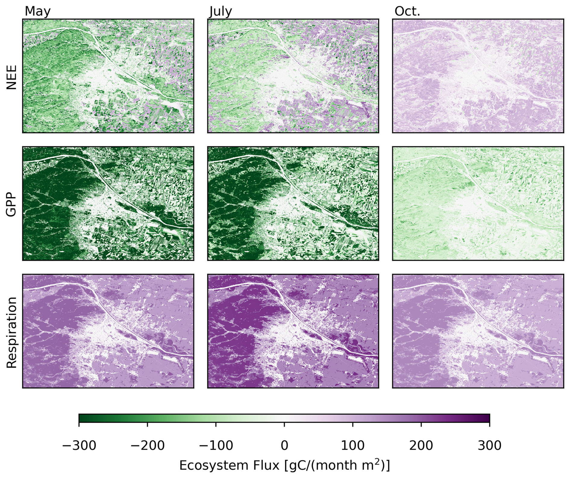
Figure 9 Monthly aggregated ecosystem fluxes for 3 months in the region around Vienna. The different months (May, July, October) are shown in the panels from left to right. From top to bottom, net ecosystem exchange (NEE), gross primary production (GPP), and respiration are shown. Negative values represent a carbon uptake, while positive fluxes show carbon release into the atmosphere. The fluxes are based on Sentinel-2 images, a hybrid land cover map, and hourly ERA5-Land meteorological data. The corresponding land cover map is shown in Fig. 4.

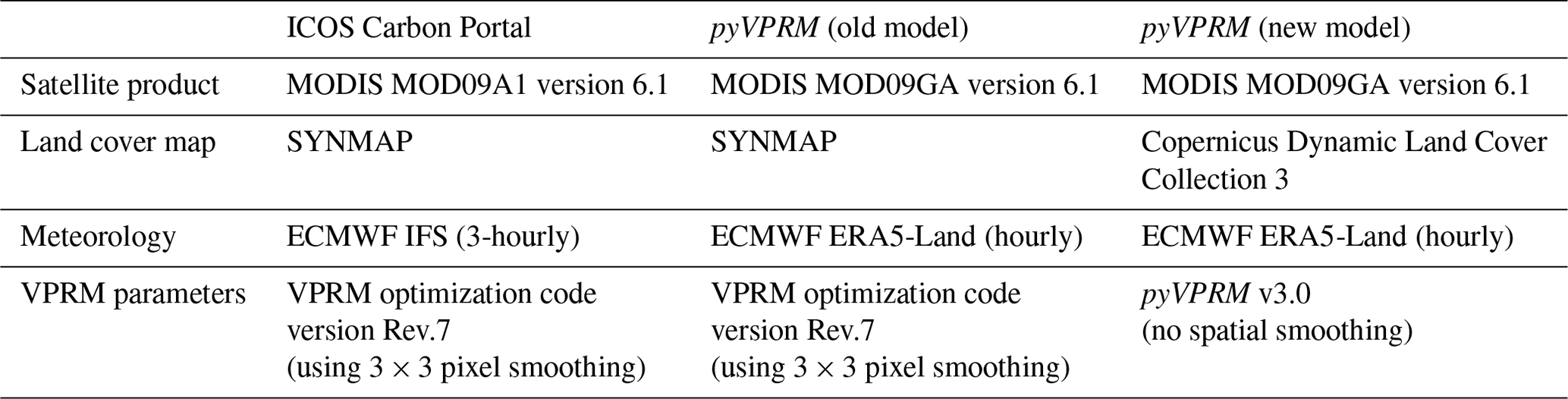
Finally, we have compared the MODIS-based European fluxes from pyVPRM against those published on the ICOS Carbon Portal for the year 2023 (ICOS RI et al., 2023); see Fig. 12. A summary of the model properties for the different flux datasets is shown in Table 4. The plot on the left shows the annual net carbon flux as published on the ICOS Carbon Portal using the old software and old model settings. The middle panel shows a model run with the same VPRM parameters and the same land cover maps as the old version but using the pyVPRM to run the computations. The comparison shows that the old and new software frameworks produce numerically compatible results. The right panel shows the annual fluxes using pyVPRM and the new VPRM parameters as well as the new land cover map. This clearly shows how the fluxes change with the new approach.

Table 4 A comparison of the VPRM settings used to estimate the European carbon fluxes in Fig. 12.

6 Discussion

Evidently, fluxes change significantly with the new VPRM version. This is primarily driven by improvements in the VPRM parameter estimation for cropland and grassland. The origin of those improvements is illustrated in Fig. 10. Two changes are important here: one related to the spatial smoothing of the satellite data and one related to the fit procedure itself.

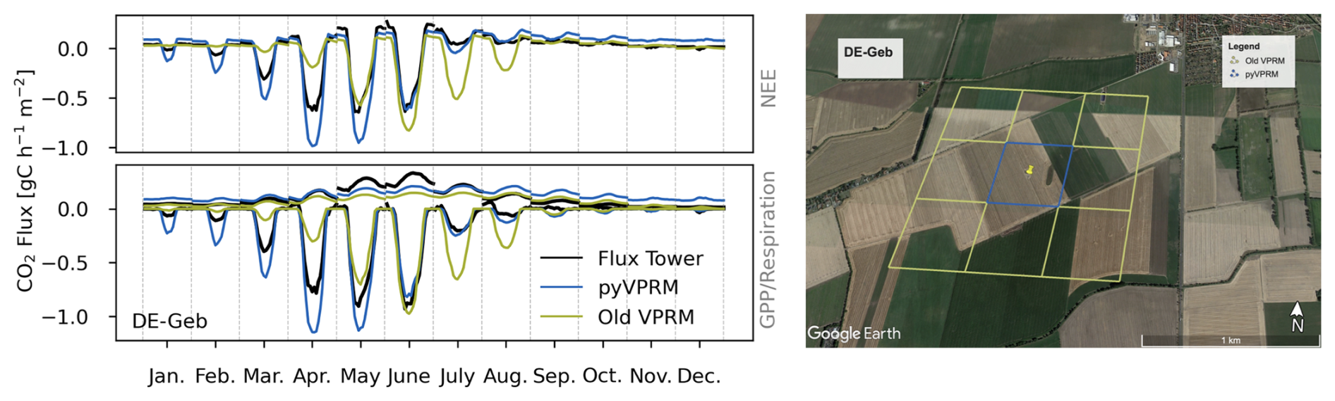
Figure 10 Left panel: the monthly mean diurnal cycles for NEE (top plot) and for respiration and GPP (bottom plot) for the cropland site Gebesee (DE-Geb; 51.0997° N, 10.9146° E) in 2007. Flux tower data are shown as solid black lines, and VPRM estimates from the old and new model are shown as green and blue lines, respectively. The flux partitioning is based on the nighttime partitioning method with a variable u^* threshold. GPP is shown as negative fluxes (carbon uptake), and respiration as positive values (carbon release). Right panel: image of the DE-Geb site. The blue square shows the MODIS pixel on top of the flux tower location (yellow pin). The green pixels show the satellite data used in the previous VPRM version. © Google Earth 2024.

First, the old VPRM version used a 3×3 spatial smoothing of the MODIS data before the fit, while pyVPRM does not. The difference becomes particularly visible for heterogeneous land cover types – in Europe especially for grassland and cropland. Figure 10 shows an example of this for the Gebesee (DE-Geb; 51.0997° N, 10.9146° E) cropland site. A single MODIS pixel on top of the flux tower already covers more than one field. Consequently, doing a 3×3 pixel smoothing includes many fields, diluting the seasonal cycle of the EVI (see also Fig. 2). As a result, the new GPP model, which does not use spatial smoothing, better matches the observations (Fig. 10).

The second key difference between the versions is that the pyVPRM fit follows a two-step procedure: at the beginning, the respiration parameters are fitted against nighttime (respiration) measurements, and then the GPP parameters are fitted using (daytime) NEE data (utilizing the previously fitted respiration parameters). The old parameters, on the other hand, were produced by simultaneously fitting the GPP and respiration parameters at once using daytime and nighttime NEE data. The problem with this strategy is that errors in the GPP are propagated to the respiration, as GPP fluxes are much larger and more variable than those of respiration. In the case of Gebesee (DE-Geb; 51.0997° N, 10.9146° E), the underestimation of the GPP forces the respiration to also be underestimated to better match the NEE.

In summary, this shows that it is important to (1) match the spatial smoothing of the satellite data to the flux tower footprint and (2) to fit respiration and GPP separately to avoid systematic biases. As a consequence, the slope of the new respiration function, α in Eq. (9), is 3 times higher for grasslands and croplands than the previously reported parameters (Gerbig, 2024) and therefore much more in line with the respiration parameters for the other vegetation classes. Figure 11 shows the respiration function for the grasslands sites for the old and the new version of VPRM (the same plot for the cropland sites is shown in the Appendix, Fig. F1). The respiration function in the old version underestimates the carbon release to the atmosphere for most of the sites. The deviation becomes especially large for high-respiration periods (i.e., high-temperature periods). While it is evident that the simple linear respiration function does not capture all effects of the ecosystem respiration, the new function is clearly an improvement over the old version. This has large implications for European flux estimates, as croplands and grassland make up 39 % and 15 % of the total European land surface area, respectively (Buchhorn et al., 2020).

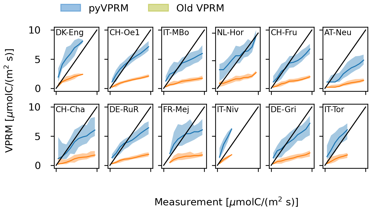
Figure 11 Comparison of VPRM respiration models and eddy-covariance measurements for the old VPRM model and the new pyVPRM model at the grassland sites. For the measurements data, the partitioned variable “RECO_NT_VUT_REF” has been used. The bands show the 10th and 90th percentiles of the model. The black solid line is the expectation for a perfect model.

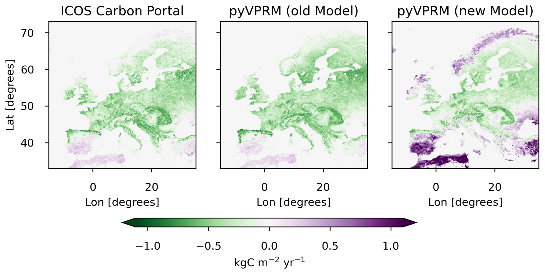
Figure 12 Annual NEE for Europe in 2023 at a 0.25°×0.25° resolution. Negative flux values (green) show a net carbon uptake, while positive values (purple), a net carbon release. Left panel: fluxes taken from the ICOS Carbon Portal (Gerbig and Koch, 2024). Middle panel: fluxes generated with pyVPRM but using the same VPRM parameters and land cover map (SYNMAP) as for the fluxes in the ICOS Carbon Portal. Right panel: fluxes calculated using the new pyVPRM implementation with the new land cover map and MODIS VPRM parameters as given in Table 3.

Overall the annual NEE budget for the European domain in 2023 changes by 75 %, from −2.1 PgC yr⁻¹ (ICOS Carbon Portal (Gerbig and Koch, 2024)) to −0.45 PgC yr⁻¹ (new pyVPRM estimate). The former is likely an overestimation of the carbon sink, caused by the underestimation of respiration. Our new pyVPRM budget, on the contrary, is more consistent with previous works estimating the European carbon sink (Monteil et al., 2020; Munassar et al., 2022; Crowell et al., 2019; Scholze et al., 2019). Monteil et al. (2020) provides a comprehensive intercomparison study of different inversion systems with varying transport models, inversion approaches, and priors for the European domain. For most prior biogenic flux models, the estimate carbon sink is between −0.5 and 0 PgC yr⁻¹. A much larger sink is estimated only when using the old VPRM fluxes as the prior, which is likely related to the respiration issue discussed above. By assimilating three datasets (in situ atmospheric CO₂, remotely sensed soil moisture, and vegetation optical depth), Scholze et al. (2019) estimate a carbon sink of $-\mathrm{0.3}\pm \mathrm{0.08}$ PgC yr⁻¹. Crowell et al. (2019) use OCO-2 XCO2 data in an inversion system and estimate the sink as $-\mathrm{0.25}\pm \mathrm{0.46}$ PgC yr⁻¹.

As expected, the changes from the old to the new VPRM estimate are mainly driven by changes in the budget of grassland and cropland. In both cases, the carbon sink decreases by around 0.7 PgC yr⁻¹. Cropland is estimated to be a sink with −0.16 PgC yr⁻¹. Grassland, on the contrary, turns into a source of around 0.4 PgC yr⁻¹. This is clearly visible in Scandinavia, around the Mediterranean, and in northern Africa. Assuming a closed carbon cycle, this is an indication that some model issues also remain in the new VPRM version. Especially unrealistic are net respiration fluxes in low soil and biomass carbon regions in southern Spain up to nearly 1 kgC m² yr⁻¹. As a second-order effect, the sink of evergreen forests is reduced by around 0.4 PgC yr⁻¹.

There are different limitations in the current VPRM model that could explain inaccuracies: (1) the sparse coverage of eddy-covariance towers, especially in Scandinavia, Spain, and the Balkans, does not provide strong constraints on the VPRM parameters in these regions. Hence, the VPRM parameters from central Europe are extrapolated to regions and climates where they likely have limited applicability. This problem appears to be smaller in the previous VPRM version because of the underfitted respiration parameters; see Fig. 11. (2) The linear respiration function is likely unrealistic for high temperatures and low soil moisture levels. Recent studies suggest that unimodal respiration functions might provide a better description under these conditions (Niu et al., 2024). (3) The respiration function currently does not take into account the total amount of plants and biomass available. This problem can be tackled by including EVI in the respiration as shown in (Gourdji et al., 2022). An implementation of this modified VPRM is available in the pyVPRM GitHub repository (https://github.com/tglauch/pyVPRM/tree/main, last access: 24 July 2025) but not discussed in this paper. Improvements for the respiration function will be investigated and implemented in future versions of pyVPRM. Finally, grasslands pose a special challenge, as they can be managed/unmanaged, xeric/non-xeric, and high/low altitude. Most European flux tower sites currently measure managed grasslands in central Europe. Adding flux towers in the dry (Mediterranean) and polar (Scandinavian) regions might facilitate calculation of the VPRM parameters for those different types of grasslands.

A central improvement of pyVPRM is the ability to use different satellite and land cover data products depending on the application. While MODIS and VIIRS provide long-term observations at 500 m resolution, Sentinel-2 is especially applicable for high-resolution applications like the modeling of urban fluxes. Especially for heterogeneous land cover types such as croplands and grasslands, the new VPRM parameters enhance the coherence between the model and flux tower data. However, the current VPRM parameter estimation still has limitations. Notably, it does not account for the time-dependent footprint of the flux towers, which remains a key area for improvement in future research.

7 Conclusions

pyVPRM provides a next-generation framework for the application of the Vegetation Photosynthesis and Respiration Model (VPRM) from city to continental scale. The model is driven by remote sensing indices and meteorological variables to estimate the ecosystem's light-use efficiency for the uptake of carbon through photosynthesis and the (temperature-dependent) ecosystem respiration. Typical applications are the estimation of ecosystem carbon budgets from city to global scale and as a biospheric prior for the estimation of both biogenic and anthropogenic CO₂ emissions using atmospheric inversion with transport models like WRF-GHG (Beck et al., 2012) or ICON-ART (Schröter et al., 2018).

pyVPRM extends previous VPRM versions (Mahadevan et al., 2008) by including the latest remote sensing products from Sentinel-2 and VIIRS, as well as updated and dynamic land cover products like the global Copernicus Dynamic Land Cover Collection 3 and the global ESA WorldCover. Using Sentinel-2 data enables us, for the first time, to resolve very heterogeneous landscapes like croplands, agricultural grasslands, or urban areas. Using VIIRS as a replacement for MODIS guarantees consistent long-term datasets after the planned discontinuation of MODIS. Furthermore, pyVPRM brings improvements in the model parameterization of grasslands and shrublands compared to the current implementation in the ICOS Carbon Portal (Gerbig, 2024).

Free model parameters for eight ecosystem types are fitted using data from up to 97 eddy-covariance towers across Europe. Comparing to flux tower data we observe significant improvements with the Sentinel-2 model, due to a better representation of the flux tower footprint. This is most important for cropland and grassland sites, which are heterogeneous vegetation classes that are very abundant in Europe.

In contrast to previous MODIS-based flux estimates for the European domain (Gerbig and Koch, 2021), pyVPRM has a more realistic overall budget when compared to independent top-down estimates (Monteil et al., 2020) and improves the seasonal and diurnal cycle for grassland and cropland. This is mostly related to the improved fitting procedure, in which the estimation of the respiration function is not influenced by mismatches between the measured GPP and the EVI estimation. Smaller improvements come from the usage of a higher-resolution land cover map and the replacement of the 3-hourly ECMWF IFS model (Roberts et al., 2018) with the hourly and higher-resolution ERA5-Land reanalysis (Muñoz Sabater et al., 2021).

Due to its modular structure, pyVPRM can be easily extended to incorporate other satellite missions, meteorological models, and land cover classifications. Likewise, different versions of the VPRM model can be implemented, e.g., the modified VPRM that includes nonlinear respiration terms (Gourdji et al., 2022) or the urban VPRM, which has been optimized for applications inside of urban areas (Hardiman et al., 2017). Likewise, we can use the pyVPRM framework to run machine-learning-based models.

Appendix A: Code structure

For examples on how pyVPRM can be used, hands-on example scripts are available on GitHub (https://github.com/tglauch/pyVPRM_examples/tree/main, last access: 24 July 2025). Here, we provide a brief overview of the classes and scripts provided within pyVPRM. Two main libraries provide the interface for accessing and preprocessing the required meteorological and satellite data: pyVPRM/meteorologies and pyVPRM/sat_managers), respectively. The main preprocessing of the satellite data and land cover maps is done in the VPRM class, defined in VPRM.py. This is necessary for any kind of VPRM usage. The modules of different VPRM flux models and parameter-fitting functions are defined in the scripts in pyVPRM/vprm_models/, such as pyVPRM/vprm_models/vprm_base.py for the “base” version of the model. The interface to work with flux tower data used for parameter fitting is given in pyVPRM/lib/flux_tower_class.py, and some useful functions are provided in pyVPRM/lib/functions.py. More details about the scripts/libraries and the functions therein are provided below.

A1 pyVPRM/meteorologies

The met_data_handler classes in this folder provide an interface for the input meteorological data, which need to be customized if using a different model or data source. All meteorology classes are derived from the base class in met_base_class.py. An example to implement a new meteorology class can be found in era5_class_draft.py. met_local_measurement.py is used to extract and employ site-level meteorological data.

A2 pyVPRM/sat_managers

The satellite_data_manager class in this library is the basic data structure for all satellite image and land cover maps used in pyVPRM. It provides functions to re-project, transform, merge, and crop satellite images. All other classes for specific satellite images or land cover maps, with their respective loading routines, are derived from this base class and implemented in the respective class files in the folder.

The other scripts in this library define classes for specific satellite reflectance products (modis.py, proba_v.py, sentinel2.py, viirs.py, viirs09ga.py) or land cover maps (city.py, copernicus.py, esa_world_cover.py, mapbiomas.py, synmap.py), along with product-specific functions for data screening (e.g., for clouds, snow, and bad pixels). Configuration (YAML) files defining the VPRM vegetation classes for different land cover maps are found in pyVPRM/vprm_configs and are required to map the land cover categories to VPRM classes.

A3 VPRM.py

The VPRM class defined in VPRM.py is the implementation of the VPRM preprocessor. This is the central code to calculate the satellite indices, run the time smoothing, transform satellite data and the land cover map to the same grid, and prepare all the variables for the VPRM models. It can also be used to generate input files to run VPRM online in atmospheric models. In order to run the preprocessor, a configuration file with a mapping from land cover classes to VPRM classes is required.

A4 pyVPRM/vprm_models/vprm_base.py

In this folder, different implementations of the VPRM model are included. Every implementation requires at least a function to fit the VPRM parameters and make VPRM predictions given an instance of the VPRM preprocessor and the meteorology. The version described throughout this paper is in vprm_base.py.

A5 pyVPRM/lib/flux_tower_class.py

Flux tower data are not completely harmonized in terms of format, and as such, custom classes will likely need to be added to accommodate new data sources, and vegetation classes/land cover types may need to be harmonized by hand. Custom classes are included in this script already for FLUXNET, ICOS, AmeriFlux, and the LBA-ECO CD-32 Flux Tower Network Data Compilation. This can also be used as a template for adding new flux tower sites.

pyVPRM/lib/functions.py

Additional functions that are used in pyVPRM are stored in functions.py.

Appendix B: Data quality masking

Table B1 Flags used for data masking in MODIS. Scenes where any of the band quality, cloud masking, or cloud shadow masking criteria are not fulfilled are masked out. Scenes with an active snow flag receive special treatment; see Sect. 3.1.3.

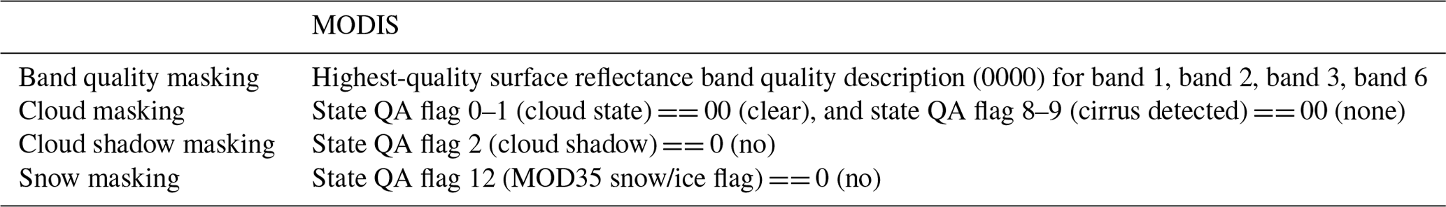
Table B2 Flags used for data masking in VIIRS. Scenes where any of the band quality, cloud masking, or cloud shadow masking criteria are not fulfilled are masked out. Scenes with an active snow flag receive special treatment; see Sect. 3.1.3.

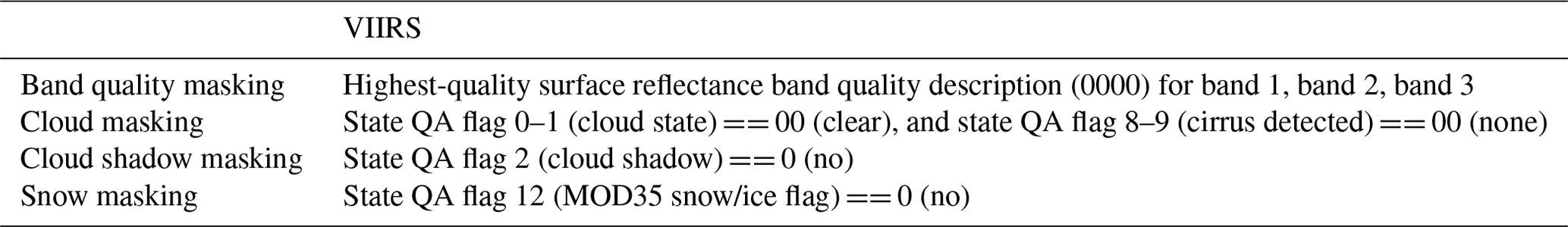
Table B3 Flags used for data masking in Sentinel-2. Scenes where any of the band quality, cloud masking, or cloud shadow masking criteria are not fulfilled are masked out. Scenes with an active snow flag receive special treatment; see Sect. 3.1.3.

Appendix C: Old VPRM parameters

Table C1 Overview of the VPRM parameter sets for MODIS used for the fluxes in the ICOS Carbon Portal (Gerbig, 2024). Abbreviations are as follows: EF – evergreen forest, DF – deciduous forest, MF – mixed forest, SHR – shrubland, SAV – Savanna, CRO – cropland, GRA – grassland.

Appendix D: Flux tower data

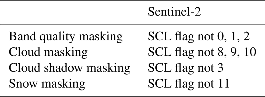
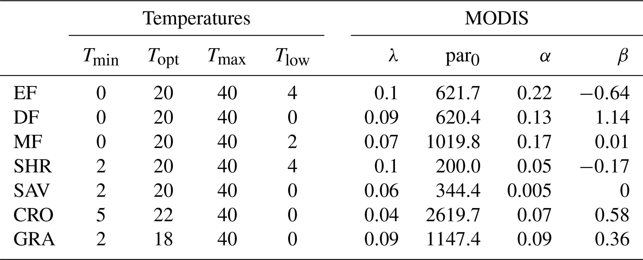
Table D1 Overview of flux tower sites and years used for estimating the VPRM parameters for MODIS, VIIRS, and Sentinel-2. Table 1/3.

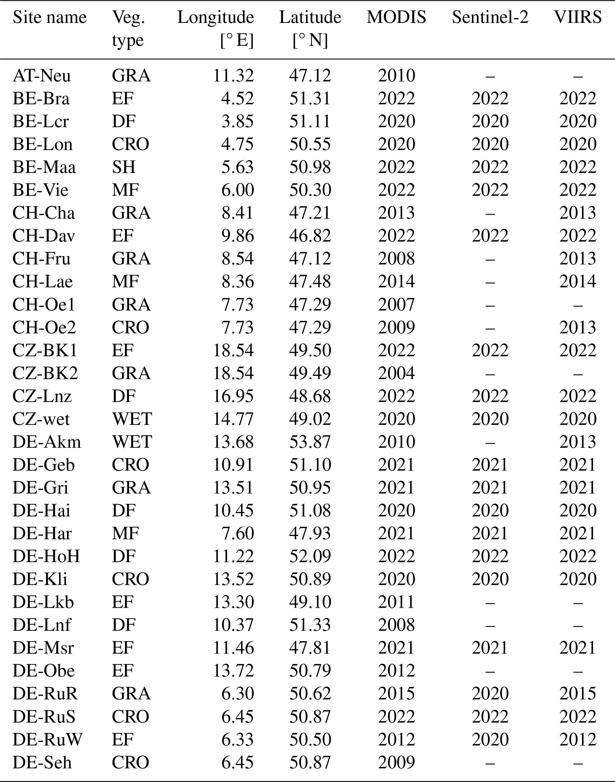
Table D2 Overview of flux tower sites and years used for estimating the VPRM parameters for MODIS, VIIRS, and Sentinel-2. Table 2/3.

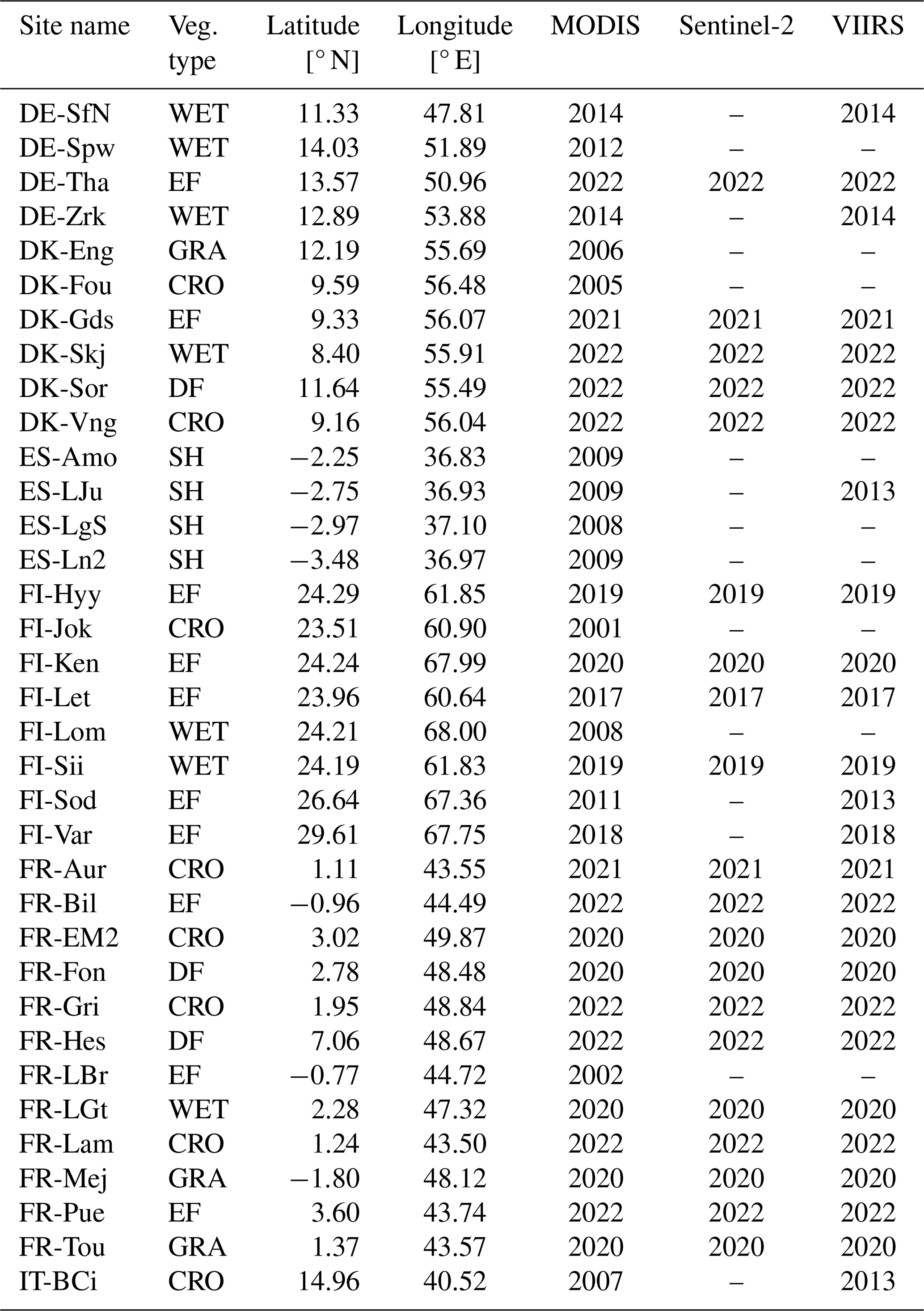
Table D3 Overview of flux tower sites and years used for estimating the VPRM parameters for MODIS, VIIRS, and Sentinel-2. Table 3/3.

Appendix E: Diurnal cycles for cropland sites

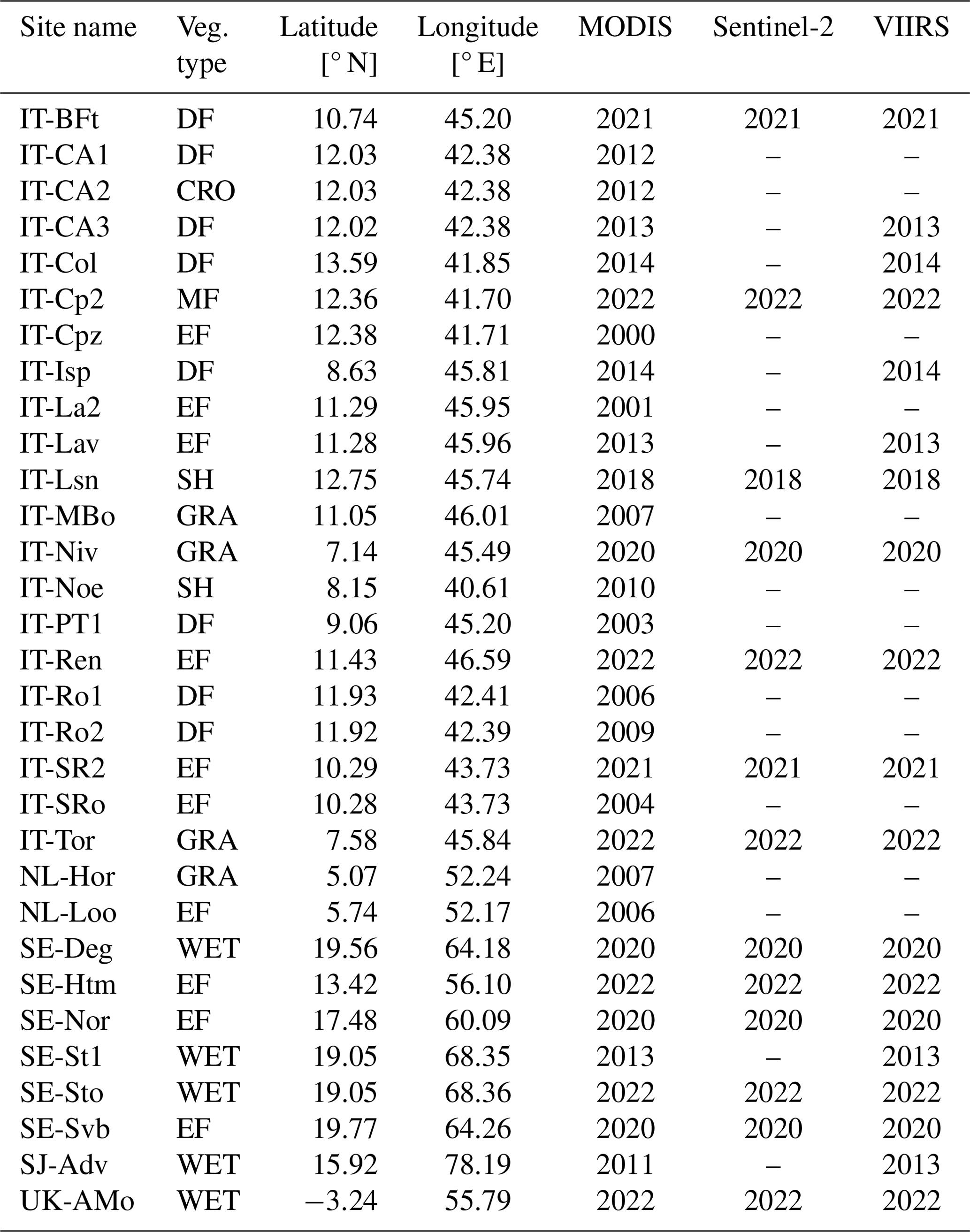
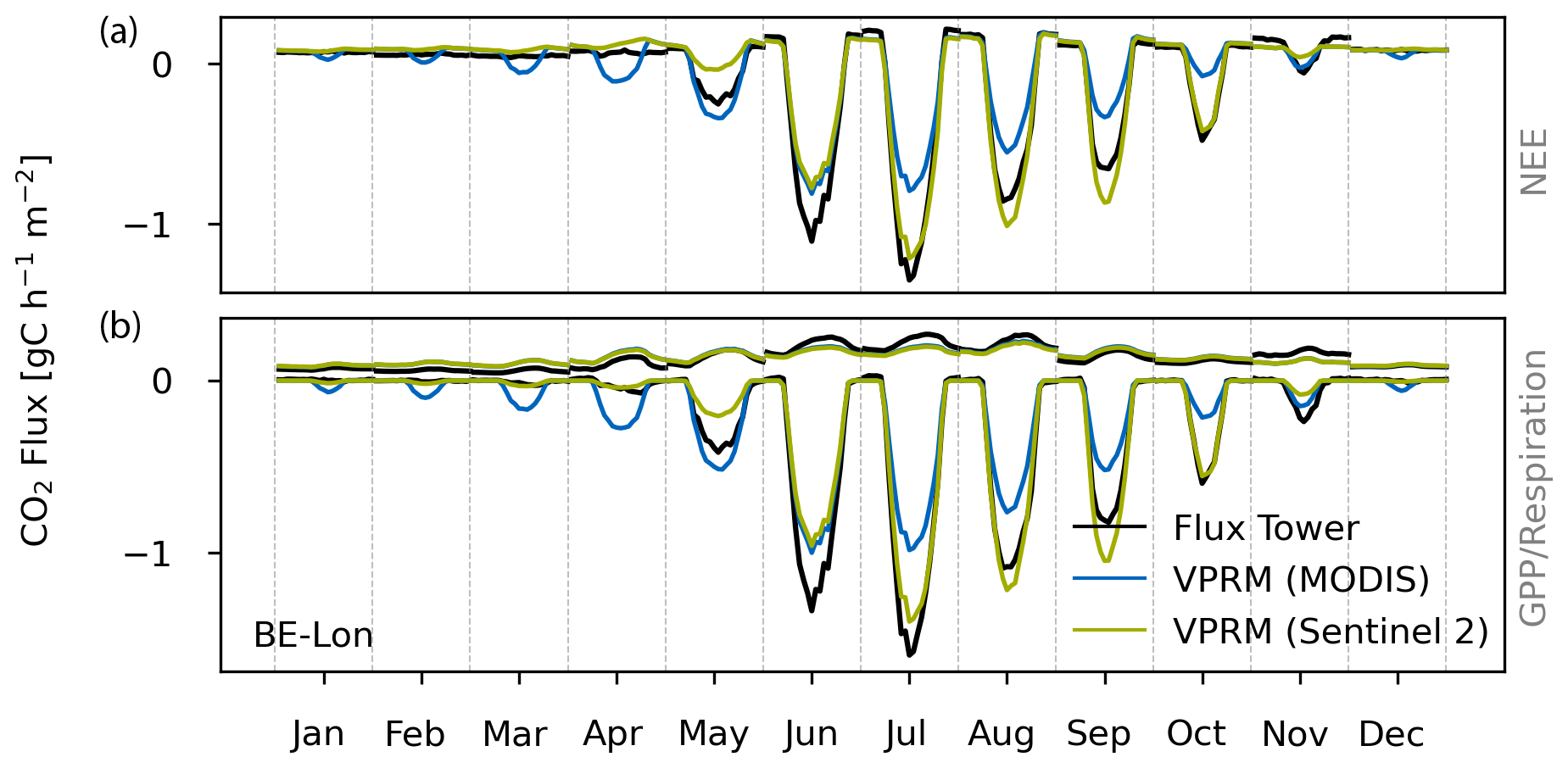
Figure E1 The mean diurnal cycle for each month at the cropland site BE-Lon. The median tower measurements for each hour of the day are shown as black lines. Colored solid lines indicate the results from the VPRM model using indices from Sentinel-2 (green) and MODIS (blue). In panel (a), NEE is shown, and in panel (b), GPP (negative values, carbon uptake) and respiration (positive values, carbon release) are shown. The flux partitioning is based on the nighttime partitioning method with a variable u^* threshold (Reichstein et al., 2005).

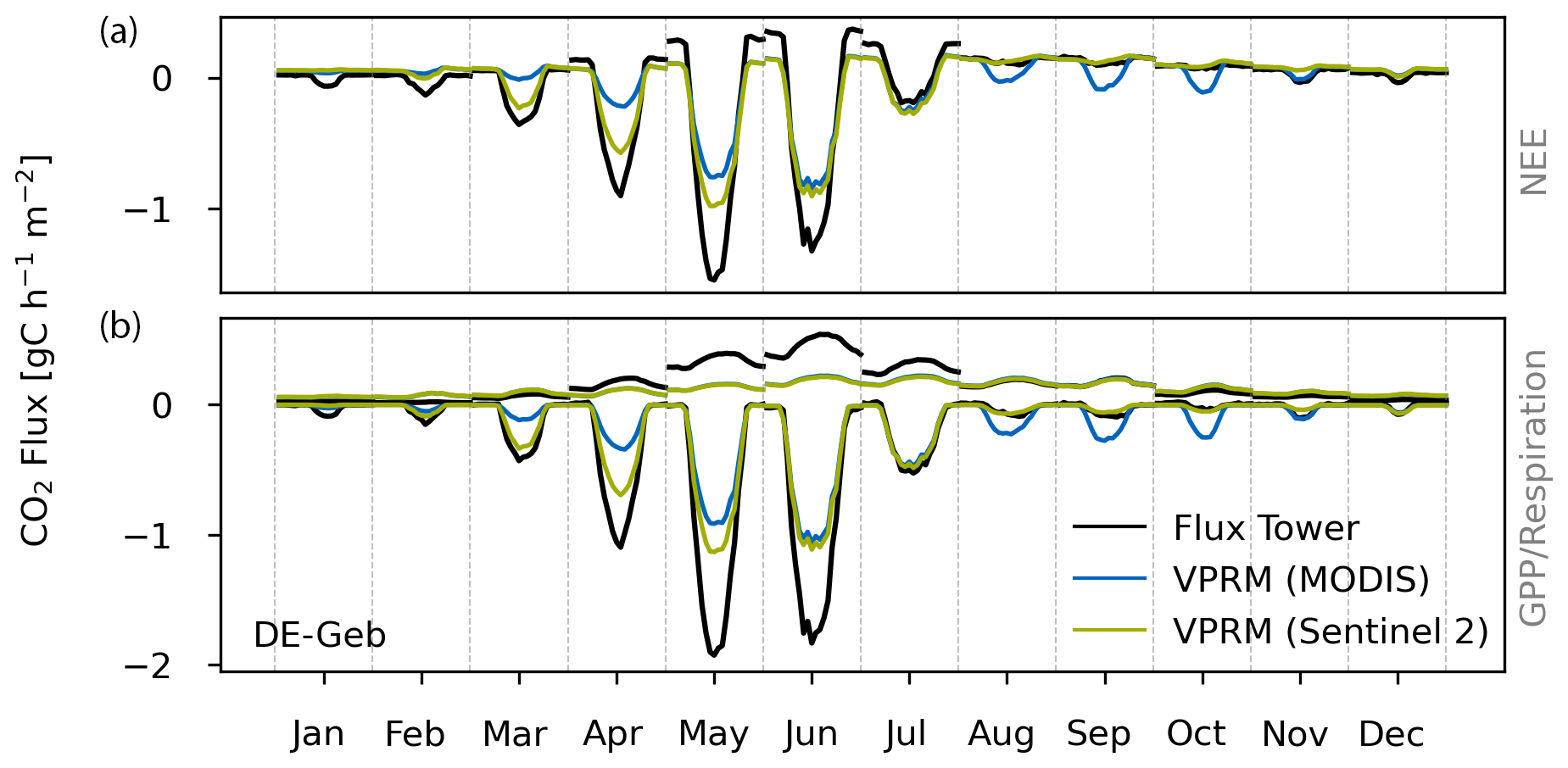
Figure E2 The mean diurnal cycle for each month at the cropland site DE-Geb. For more details, see Fig. E1.

Figure E3 The mean diurnal cycle for each month at the cropland site DE-Kli. For more details, see Fig. E1.

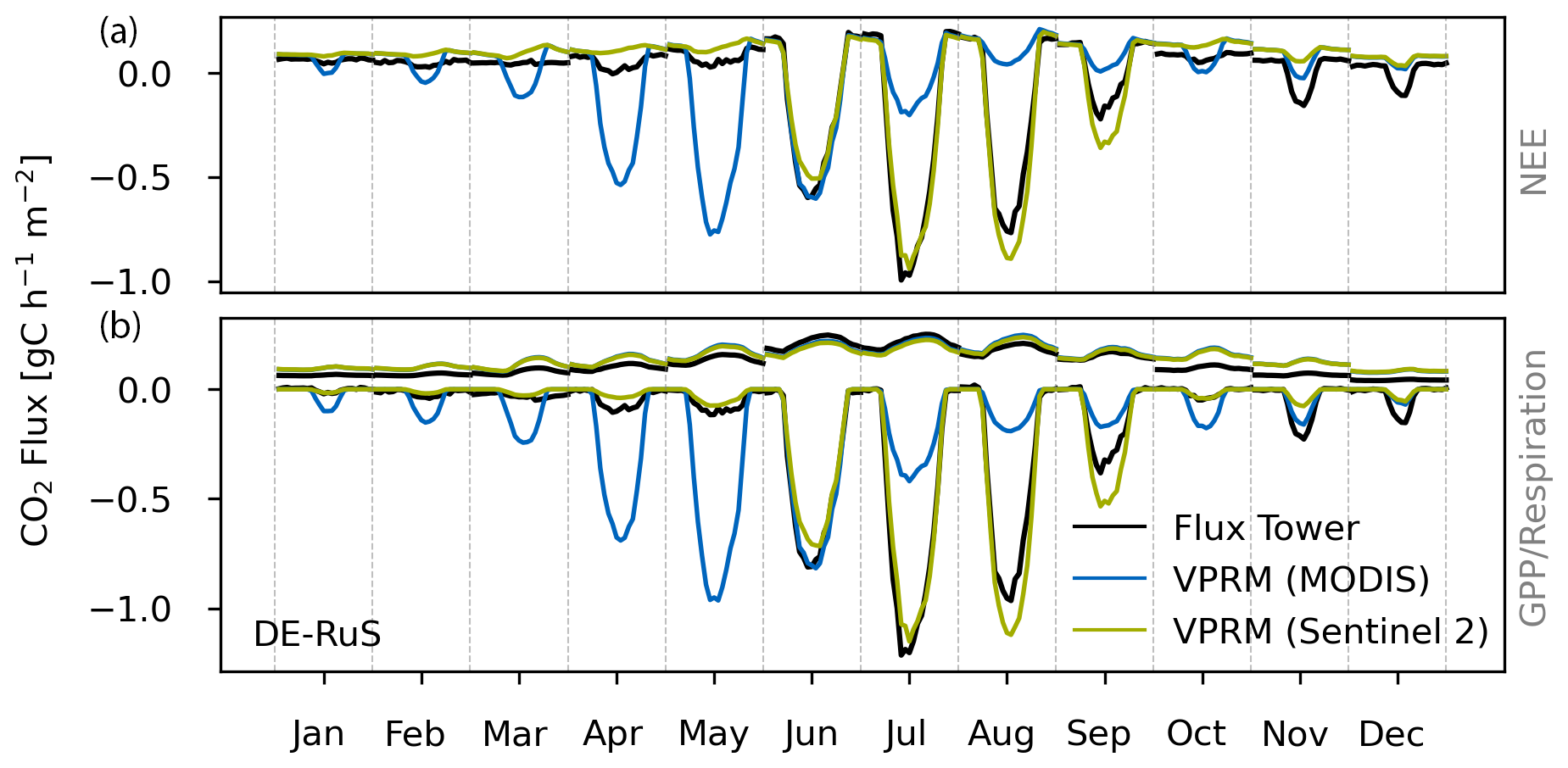
Figure E4 The mean diurnal cycle for each month at the cropland site DE-RuS. For more details, see Fig. E1.

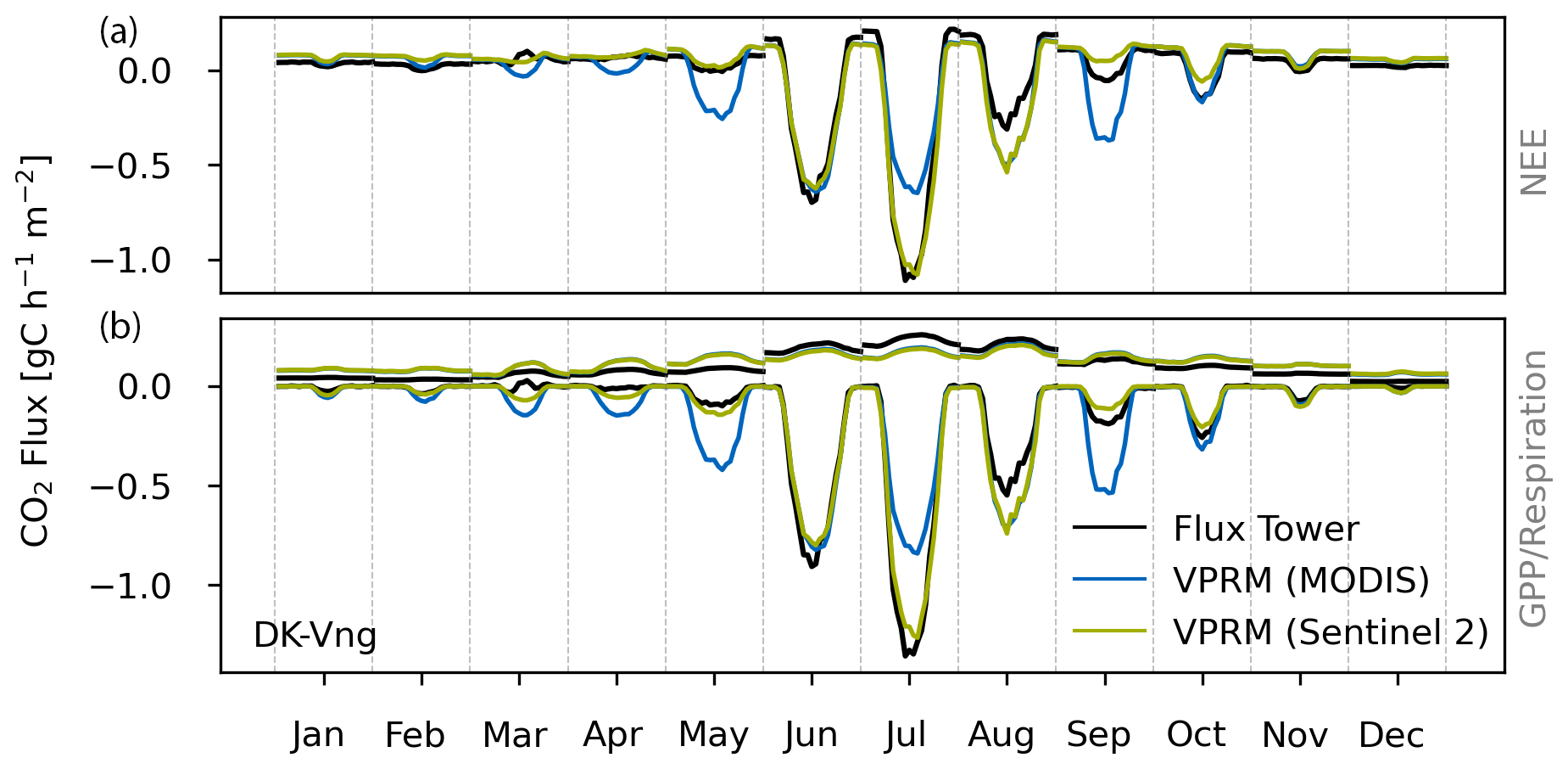
Figure E5 The mean diurnal cycle for each month at the cropland site DK-Vng. For more details, see Fig. E1.

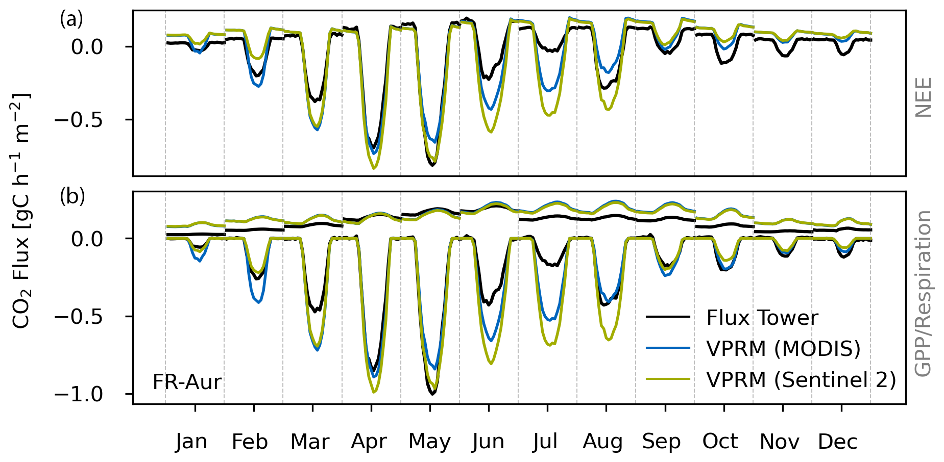
Figure E6 The mean diurnal cycle for each month at the cropland site FR-Aur. For more details, see Fig. E1.

Figure E7 The mean diurnal cycle for each month at the cropland site FR-EM2. For more details, see Fig. E1.

Figure E8 The mean diurnal cycle for each month at the cropland site FR-Gri. For more details, see Fig. E1.

Figure E9 The mean diurnal cycle for each month at the cropland site FR-Lam. For more details, see Fig. E1.

Appendix F: Respiration functions

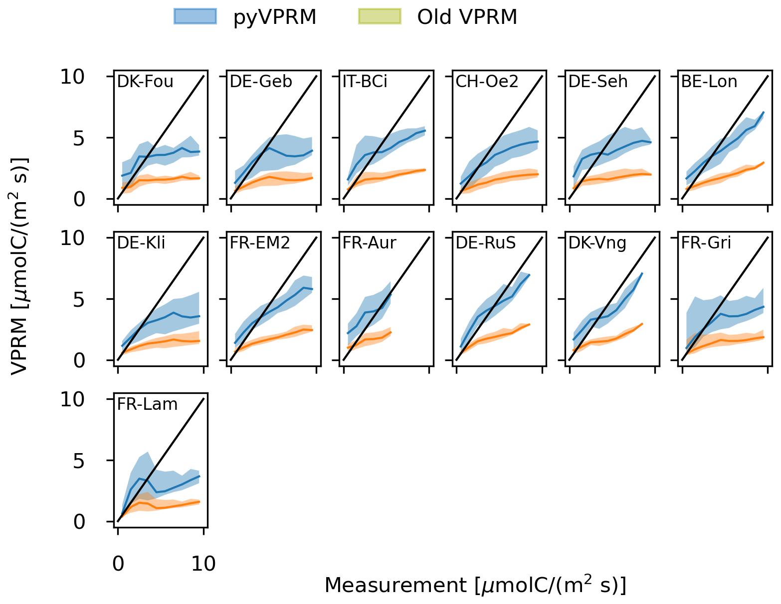
Figure F1 Comparison of VPRM respiration models and eddy-covariance measurements for the old VPRM model and the new pyVPRM model at the cropland sites. For the measurement data, the partitioned variable “RECO_NT_VUT_REF” has been used. The bands show the 10th and 90th percentiles of the model. The black solid line is the expectation for a perfect model.

Appendix G: Mean squared deviation for deciduous forest and mixed forest

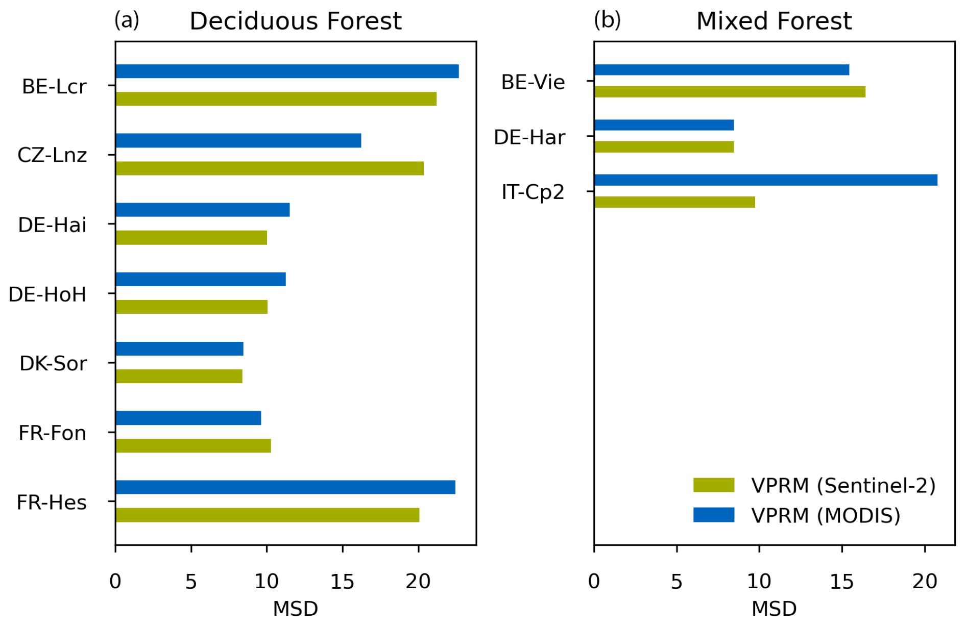
Figure G1 Mean squared deviation (MSD) between the VPRM prediction and the eddy flux tower observation for deciduous forest (a) and mixed forest (b) sites. Green and blue are used to show the VPRM predictions using Sentinel-2 and MODIS, respectively.