asQ: parallel-in-time finite element simulations using ParaDiag for geoscientific models and beyond

Modern high-performance computers are massively parallel; for many partial differential equation applications spatial parallelism saturates long before the computer's capability is reached. Parallel-in-time methods enable further speedup beyond spatial saturation by solving multiple time steps simultaneously to expose additional parallelism. ParaDiag is a particular approach to parallel-in-time methods based on preconditioning the simultaneous time step system with a perturbation that allows block diagonalisation via a Fourier transform in time. In this article, we introduce asQ, a new library for implementing ParaDiag parallel-in-time methods, with a focus on applications in the geosciences, especially weather and climate. asQ is built on Firedrake, a library for the automated solution of finite element models, and the PETSc library of scalable linear and nonlinear solvers. This enables asQ to build ParaDiag solvers for general finite element models and provide a range of solution strategies, making testing a wide array of problems straightforward. We use a quasi-Newton formulation that encompasses a range of ParaDiag methods and expose building blocks for constructing more complex methods. The performance and flexibility of asQ is demonstrated on a hierarchy of linear and nonlinear atmospheric flow models. We show that ParaDiag can offer promising speedups and that asQ is a productive testbed for further developing these methods.

1 Introduction

In this article, we present asQ, a software framework for investigating the performance of ParaDiag parallel-in-time methods. We focus our attention on geophysical fluid models relevant to the development of simulation systems for oceans, weather, and climate. This library allows researchers to rapidly prototype implementations of ParaDiag for time-dependent partial differential equations (PDEs) discretised using Firedrake (Ham et al., 2023), selecting options for the solution strategy facilitated by the composable design of PETSc, the Portable, Extensible Toolkit for Scientific Computation (Balay et al., 2024). The goal of the paper is not to advocate for ParaDiag as superior to other methods but to demonstrate that asQ serves this purpose.

Parallel-in-time (PinT) is the name for the general class of methods that introduce parallelism in the time direction as well as in space. The motivation for PinT methods is that eventually it is not possible to achieve acceptable time to solution only through spatial domain decomposition as one moves to higher and higher fidelity solutions, so one would need to look to the time dimension for further speedups. Falgout and Schroder (2023) provided a quantitative argument that any sufficiently high-resolution time-dependent simulation will eventually require the use of time-parallel methods (the question is just when and how).

PinT methods have a long history, surveyed by Gander (2015), but the topic has really exploded since the late 1990s, with many algorithms being proposed including space–time-concurrent waveform relaxation multigrid (WRMG) (Vandewalle and Van de Velde, 1994), space–time multigrid (Horton and Vandewalle, 1995), parareal (Maday and Turinici, 2002), revisionist integral deferred correction (RIDC) (Christlieb et al., 2010), multigrid reduction in time (MGRIT) (Falgout and Schroder, 2023), parallel full approximation scheme in space and time (PFASST) (Emmett and Minion, 2012), ParaEXP (Gander and Güttel, 2013), and the subject of this work – ParaDiag. As we shall elaborate later with references, ParaDiag is a computational linear algebra approach to PinT, solving an implicit system for several time steps at once, using Fourier transforms in time to obtain a block diagonal system whose components can be solved independently and in parallel. A review of the most common forms of ParaDiag and important analysis results can be found in Gander et al. (2021).

Although there are a small number of software libraries for PinT methods, most PinT software implementations are written from scratch as small standalone codes or individual scripts; increased availability and use of PinT libraries could increase research productivity (Speck and Ruprecht, 2024). At the time of writing, there are only a small number of PinT libraries that are both available open-source and general in either problems or methods treated. XBraid (XBraid, LLNL, 2025) and pySDC (Speck, 2019) are mature reference implementations of MGRIT and spectral deferred corrections, written in C and Python, respectively. These frameworks are designed to be non-intrusive, so users can plug in existing serial-in-time code to quickly experiment with these PinT methods. SWEET (Schreiber, 2018) is a testbed for time integration of the shallow water equations, a model of geophysical flow. As opposed to implementing a single family of methods for any problem, SWEET implements many methods for a specific class of problem. Nektar++ is a spectral/hp element library primarily for fluid dynamics and hyperbolic models. The parareal algorithm was recently implemented and can be used with any of the models or time integration methods supported in Nektar++ (Xing et al., 2024). Finally, the only other general ParaDiag library that the authors are aware of is pyParaDiag (Čaklović et al., 2023; Čaklović, 2023), which implements ParaDiag for collocation time integration schemes with space–time parallelism. pyParaDiag implements a few common models, and users can implement drivers for both new linear or nonlinear models. In comparison to these libraries, asQ implements a particular class of method (ParaDiag), for a particular class of discretisation (finite elements) but for general PDEs.

For the purposes of later discussion, we briefly define two scaling paradigms when exploiting parallelism. Strong scaling is where a larger number of processors are used to obtain the same solution in a shorter wall-clock time. Weak scaling is where a larger number of processors are used to obtain a higher-resolution solution in the same wall-clock time.

The rest of this article is structured as follows. In Sect. 1.1 we survey the varying PinT approaches to geophysical fluids models in particular, which incorporate transport and wave propagation processes that exhibit the general challenge of PinT methods for hyperbolic problems (and hence we also discuss aspects of hyperbolic problems more broadly). In Sect. 1.2, we complete this introduction with a survey of previous research on the ParaDiag approach to PinT. Then, in Sect. 2 we review the basic ParaDiag idea and discuss the extension to nonlinear problems, which are more relevant to weather and climate, highlighting the wide range of choices that need to be made when using ParaDiag for these problems. In Sect. 3, we describe the asQ library and explain how it addresses the need to rapidly explore different options in a high-performance computing environment. In Sect. 4 we present some numerical examples to demonstrate that we have achieved this goal. Finally, in Sect. 5 we provide a summary and outlook.

1.1 Parallel-in-time methods for hyperbolic and geophysical models

The potential for PinT methods in oceans, weather, and climate simulation is attractive because of the drive to higher resolution. For example, the Met Office Science Strategy (The Met Office, 2022) and Bauer et al. (2015) highlight the need for global convection-permitting atmosphere models, eddy-resolving ocean models, eddy-permitting local area atmosphere models, and estuary-resolving shelf-sea models, to better predict hazards and extremes, which will require sub-10 km global resolution. In operational forecasting, the model needs to run to a particular end time (e.g. 10 simulation days) within a particular wall-clock time in order to complete the forecasting procedure in time for the next cycle (e.g. three wall-clock hours). Similarly, climate scientists have a requirement for simulations to complete within a feasible time for a model to be scientifically useful. To try to maintain the operational wall-clock limit when resolution is increased, weak scaling is used so that each time step at the higher spatial resolution can be completed in the same wall-clock time as the time step at the lower spatial resolution. However, even when this weak scaling is achievable, high spatial resolution yields dynamics (e.g. transport and waves) with higher temporal frequencies that should be resolved in the time step (and sometimes we are forced to resolve them due to stability restrictions in time-stepping methods). This means that more time steps are required at the higher resolution than the lower resolution. To satisfy the operational wall-clock limit, we now need to be able to strong scale the model to reduce the wall-clock time for each time step so that the same simulation end time can be reached without breaking the wall-clock time limit at the higher resolution. Achieving this scaling with purely spatial parallelism is very challenging because these models are already run close to the scaling limits. This motivates us to consider other approaches to time stepping such as PinT methods.

The challenge to designing effective PinT methods for these geophysical fluid dynamics models is that their equations support high-frequency wave components coupled to slow balanced motion that governs the large-scale flow, such as the fronts, cyclones, jets, and Rossby waves that are the familiar features of midlatitude atmospheric weather. The hyperbolic nature of these waves makes them difficult to treat efficiently using the classical parareal algorithm, as discussed in Gander (2015). The difficulty is that the errors are dominated by dispersion error, and there is a mismatch in the dispersion relation between coarse and fine models (Ruprecht, 2018). Similarly, De Sterck et al. (2024c) showed that standard MGRIT has deteriorated convergence for hyperbolic problems due to the removal of some characteristic components on the coarse grid if simple rediscretisation is used. However, De Sterck et al. (2023a) showed that a carefully modified semi-Lagrangian method can overcome this deficiency by ensuring that the coarse-grid operator approximates the fine-grid operator to a higher order of accuracy than it approximates the PDE, analogously to previous findings for MGRIT applied to chaotic systems (Vargas et al., 2023). Using this approach, De Sterck et al. (2023b, a) demonstrated real speedups for the variable coefficient scalar advection. Scalable iteration counts were obtained for nonlinear PDEs using a preconditioned quasi-Newton iteration (De Sterck et al., 2024a) and systems of linear and nonlinear PDEs (De Sterck et al., 2024b). Hamon et al. (2020) and Caldas Steinstraesser et al. (2024) have demonstrated parallel speedups for the nonlinear rotating shallow water equations (a prototypical highly oscillatory PDE for geophysical fluid dynamics), using multilevel methods.

For linear systems with pure imaginary eigenvalues (e.g. discretisations of wave equations), a parallel technique based on sums of rational approximations of the exponential function (referred to in later literature as rational exponential integrators (REXI)) restricted to the imaginary axis was proposed in Haut et al. (2016). The terms in the sum are mutually independent, so they can be evaluated in parallel. Each of these terms requires the solution of a problem that resembles a backward Euler integrator with a complex-valued time step. For long time intervals in the wave equation case, some of these problems resemble shifted Helmholtz problems with coefficients close to the negative real axis and far from the origin. These problems are known to be very unsuited to be solved by multigrid methods which are otherwise a scalable approach for linear time-stepping problems (Gander et al., 2015). Haut et al. (2016) avoided this by using static condensation techniques for higher-order finite element methods. This approach was further investigated and developed in the geophysical fluid dynamics setting using pseudospectral methods (including on the sphere) in Schreiber et al. (2018) and Schreiber and Loft (2019). In Schreiber et al. (2019), a related approach using coefficients derived from Cauchy integral methods was presented. In an alternative direction, ParaEXP (Gander and Güttel, 2013) provides a PinT mechanism for dealing with nonzero source terms for the linear wave equation, if a fast method for applying the exponential is available.

Multiscale methods are a different strategy to tackle the highly oscillatory components, whose phases are not tremendously important, but their bulk coupling to the large scale can be. Legoll et al. (2013) proposed a micro–macro parareal approach where the coarse propagator is obtained by averaging the vector field over numerical solutions with frozen macroscopic dynamics, demonstrating parallel speedups for test problems using highly oscillatory ordinary differential equations. Haut and Wingate (2014) proposed a different approach, based on previous analytical work (Schochet, 1994; Embid and Majda, 1998; Majda and Embid, 1998), in which the highly oscillatory PDE is transformed using operator exponentials to a nonautonomous PDE with rapidly fluctuating explicit time dependence. After averaging over the phase of this explicit time dependence, a slow PDE is obtained that approximates the transformed system under suitable assumptions. To obtain a numerical algorithm, the “averaging window” (range of phase values to average over) is kept finite, and the average is replaced by a sum whose terms can be evaluated independently in parallel (providing parallelisation across the method for the averaged PDE). Haut and Wingate (2014) used this approach to build a coarse propagator for the one-dimensional rotating shallow water equations. In experiments with a standard geophysical fluid dynamics test case on the sphere, Yamazaki et al. (2023) showed that the error due to averaging can actually be less than the time discretisation error in a standard method with the same time step size, suggesting that phase averaging might be used as a PinT method in its own right without needing a parareal iteration to correct it. Bauer et al. (2022) showed an alternative route to correcting the phase averaging error using a series of higher-order terms, which may expose additional parallelism.

1.2 Prior ParaDiag research

The software we present here is focused on α-circulant diagonalisation techniques for all-at-once systems, which have come to be known in the literature as “ParaDiag”. In this class of methods, a linear constant coefficient ODE (e.g. a discretisation in space of a linear constant coefficient PDE) is discretised in time, resulting in a system of equations with a tensor product structure in space and time. This system is then diagonalised in time, leading to a block diagonal system with one block per time step, which can each be solved in parallel before transforming back to obtain the solution at each time step. The first mathematical challenge is that the block structure in time is not actually diagonalisable for constant time step Δt because of the nontrivial Jordan normal form. In the original paper on diagonalisation in time, Maday and Rønquist (2008) tackled this problem by using time steps forming a geometric progression, which then allows for a direct diagonalisation. The main drawback is that the diagonalisation is badly conditioned for small geometric growth rate, which might otherwise be required for accurate solutions. McDonald et al. (2018) proposed to use a time-periodic (and thus diagonalisable) system to precondition the initial value system. This works well for parabolic systems but is not robust to mesh size for wave equations (such as those arising in geophysical fluid applications). Gander and Wu (2019) (following Wu (2018) in the parareal context) proposed a modification, in which the periodicity condition u(0)=u(T) is replaced by a periodicity condition $u^k\left(\mathrm{0}\right)=u_{\mathrm{0}}+\mathit{\alpha }\left(u^k\right(T)-u^{k-\mathrm{1}}(T\left)\right)$ in the preconditioner, with u₀ the real initial condition, k the iteration index, and $\mathrm{0}<\mathit{\alpha }<\mathrm{1}$, with the resulting time block structure being called α-circulant. This system can be diagonalised by fast Fourier transform (FFT) in time after appropriate scaling by a geometric series. When $\mathit{\alpha }<\frac{\mathrm{1}}{\mathrm{2}}$, an upper bound can be shown for the preconditioner, which is independent of the mesh, the linear operator, and any parameters of the problem. In particular, it produces mesh-independent convergence for the wave equation. However, the diagonalisation is badly conditioned in the limit α→0 (Gander and Wu, 2019). Čaklović et al. (2023) addressed this by adapting α at each iteration.

The technique has also been extended to other time-stepping methods. Čaklović et al. (2023) provided a general framework for higher-order implicit collocation methods, using the diagonalisation of the polynomial integral matrix. The method can also be extended to higher-order multistep methods, such as backward difference formulae (BDF) methods (Danieli and Wathen, 2021; Gander and Palitta, 2024) or Runge–Kutta methods (Wu and Zhou, 2021; Kressner et al., 2023).

Moving to nonlinear PDEs, the all-at-once system for multiple time steps must now be solved using a Newton or quasi-Newton method. The Jacobian system is not a constant coefficient in general, so it must be approximated by some form of average, as first proposed by Gander and Halpern (2017). There are a few analytical results about this approach. Gander and Wu (2019) proved convergence for a fixed-point iteration for the nonlinear problem when an α-periodic time boundary condition is used. Čaklović (2023) developed a theory for convergence of quasi-Newton methods, presented later in Eq. (25).

Performance measurements for time-parallel ParaDiag implementations are still relatively sparse in the literature and have been predominantly for linear problems with small-scale parallelism. Goddard and Wathen (2019), Gander et al. (2021), and Liu et al. (2022) found very good strong scaling up to 32, 128, and 256 processors respectively for the heat, advection, and wave equations, with Liu et al. (2022) noting the importance of a fast network for multi-node performance due to the collective communications required in ParaDiag. Actual speedups vs. a serial-in-time method of 15× were obtained by Liu and Wu (2020) for the wave equation on 128 processors. A doubly time-parallel ParaDiag implementation was presented in Čaklović et al. (2023) for the collocation method with parallelism across both the collocation nodes and the time steps. For the heat and advection equations, they achieved speedups of 15–20× over the serial-in-time/serial-in-space method on 192 processors and speedups of 10× over the serial-in-time/parallel-in-space method on 2304 processors (with a speedup of 85× over the serial-in-time/serial-in-space method). As far as the authors are aware, the study of Čaklović (2023) is the only one showing speedups vs. a serial-in-time method for nonlinear problems, achieving speedups of 25× for the Allen–Cahn equations and speedups of 5.4× for the hyperbolic Boltzmann equation.

2 ParaDiag methods

In this section we review the ParaDiag method. First, we discuss application to linear problems for which it was originally developed. Second, we discuss the adaptation to nonlinear problems which are of interest in many practical applications. We then use a simple performance model to highlight the requirements for ParaDiag to be an effective method.

ParaDiag is a method to accelerate the solution of an existing time integrator, so we will define the serial-in-time method first. In our exposition, we are interested in time-dependent (and initially linear with constant coefficient) PDEs combined with a finite element semi-discretisation in space:

$$\begin{array}{}\text{(1)}& M{\partial }_{t}u+Ku=b\left(t\right),\end{array}$$

where $u\in {\mathbb{R}}^{N_x}$ is the unknown, $M\in {\mathbb{R}}^{N_x\times N_x}$ is the mass matrix, $K\in {\mathbb{R}}^{N_x\times N_x}$ is the stiffness matrix arising from the discretisation of the spatial terms, $b\left(t\right)\in {\mathbb{R}}^{N_x}$ is some forcing term not dependent on the solution, and N_x is the number of spatial degrees of freedom (DoFs). Throughout Sect. 2.1 and 2.2, lower-case Roman letters denote vectors (except t, which is reserved for time, and n and j, which are reserved for integers); upper-case Roman letters denote matrices (except N, which is reserved for integers); vectors and matrices defined over both space and time are in boldface; and Greek letters denote scalars. Equation (1) is solved on a spatial domain x∈Ω with appropriate boundary conditions on the boundary ∂Ω. We want to find the solution in the time range $t\in \left[t_{\mathrm{0}},t_{\mathrm{0}}+T\right]$ with T=N_tΔt, starting from an initial condition u₀=u(t₀) at time t₀. To achieve this, Eq. (1) is discretised in time using the implicit θ-method:

$$\begin{array}{}\text{(2)}& {\displaystyle \frac{\mathrm{1}}{\mathrm{\Delta }t}}M\left(u^{n+\mathrm{1}}-u^n\right)+\mathit{\theta }K{u}^{n+\mathrm{1}}+\left(\mathrm{1}-\mathit{\theta }\right)K{u}^n={\stackrel{\mathrm{̃}}{b}}^{n+\mathrm{1}},\end{array}$$

where the right-hand side is

$$\begin{array}{}\text{(3)}& {\stackrel{\mathrm{̃}}{b}}^{n+\mathrm{1}}=\mathit{\theta }{b}^{n+\mathrm{1}}+\left(\mathrm{1}-\mathit{\theta }\right)b^n,\end{array}$$

where Δt is the time step size, $n\in [\mathrm{0},N_t]$ is the time step index, uⁿ is the discrete solution at time $t=t_{\mathrm{0}}+n\mathrm{\Delta }t$, and $\mathit{\theta }\in [\mathrm{0},\mathrm{1}]$ is a parameter. ParaDiag is not restricted to the θ method, but this is currently the only method implemented in asQ (other methods may be added in the future).

As written, Eq. (2) is an inherently serial method, requiring the solution of an implicit system for each time step uⁿ⁺¹ given uⁿ.

2.1 Linear problems

The ParaDiag method begins by constructing a single monolithic system for multiple time steps, called the “all-at-once system”. We illustrate an all-at-once system below for four time steps (N_t=4), created by combining Eq. (2) for $n=\mathrm{0},\mathrm{1},\mathrm{2},\mathrm{3}$, to obtain

$$\begin{array}{}\text{(4)}& \mathbf{A}\mathit{u}=\left(B_{\mathrm{1}}\otimes M+B_{\mathrm{2}}\otimes K\right)\mathit{u}=\stackrel{\mathrm{̃}}{\mathit{b}},\end{array}$$

where ⊗ is the Kronecker product. The all-at-once matrix $\mathbf{A}\in {\mathbb{R}}^{N_t{N}_x\times N_t{N}_x}$ (which is the Jacobian of the full all-at-once residual $\mathbf{A}\mathit{u}-\stackrel{\mathrm{̃}}{\mathit{b}}$) is written using Kronecker products of the mass and stiffness matrices with the two matrices $B_{\mathrm{1},\mathrm{2}}\in {\mathbb{R}}^{N_t\times N_t}$. These are Toeplitz matrices which define the time integrator:

$$\begin{array}{}\text{(5)}& {\displaystyle }{B}_{\mathrm{1}}=& {\displaystyle \frac{\mathrm{1}}{\mathrm{\Delta }t}}\left(\begin{array}{cccc}\mathrm{1}& \mathrm{0}& \mathrm{0}& \mathrm{0}\\ -\mathrm{1}& \mathrm{1}& \mathrm{0}& \mathrm{0}\\ \mathrm{0}& -\mathrm{1}& \mathrm{1}& \mathrm{0}\\ \mathrm{0}& \mathrm{0}& -\mathrm{1}& \mathrm{1}\end{array}\right),\text{(6)}& {\displaystyle }{B}_{\mathrm{2}}=& {\displaystyle }\left(\begin{array}{cccc}\mathit{\theta }& \mathrm{0}& \mathrm{0}& \mathrm{0}\\ (\mathrm{1}-\mathit{\theta })& \mathit{\theta }& \mathrm{0}& \mathrm{0}\\ \mathrm{0}& (\mathrm{1}-\mathit{\theta })& \mathit{\theta }& \mathrm{0}\\ \mathrm{0}& \mathrm{0}& (\mathrm{1}-\mathit{\theta })& \mathit{\theta }\end{array}\right),\end{array}$$

and the vector $\mathit{u}\in {\mathbb{R}}^{N_t{N}_x}$ of unknowns for the whole time series is

$$\begin{array}{}\text{(7)}& \mathit{u}=\left(\begin{array}{c}{u}^{\mathrm{1}}\\ u^{\mathrm{2}}\\ u^{\mathrm{3}}\\ u^{\mathrm{4}}\end{array}\right).\end{array}$$

The right-hand side $\stackrel{\mathrm{̃}}{\mathit{b}}\in {\mathbb{R}}^{N_t{N}_x}$ includes the initial conditions:

$$\begin{array}{}\text{(8)}& \stackrel{\mathrm{̃}}{\mathit{b}}=\left(\begin{array}{c}{\stackrel{\mathrm{̃}}{b}}^{\mathrm{1}}\\ {\stackrel{\mathrm{̃}}{b}}^{\mathrm{2}}\\ {\stackrel{\mathrm{̃}}{b}}^{\mathrm{3}}\\ {\stackrel{\mathrm{̃}}{b}}^{\mathrm{4}}\end{array}\right)+\left(\begin{array}{c}\left(\frac{\mathrm{1}}{\mathrm{\Delta }t}M-(\mathrm{1}-\mathit{\theta })K\right)u^{\mathrm{0}}\\ \mathrm{0}\\ \mathrm{0}\\ \mathrm{0}\end{array}\right).\end{array}$$

Due to the properties of the Kronecker product, if B₁ and B₂ are simultaneously diagonalisable, then the Jacobian A is block-diagonalisable. A block-diagonal matrix can be efficiently inverted by solving each block separately in parallel. Note that when forming an ${\mathbb{R}}^{N_t{N}_x\times N_t{N}_x}$ space–time matrix using a Kronecker product, the ${\mathbb{R}}^{N_t\times N_t}$ matrix is always on the left of the Kronecker product, and the ${\mathbb{R}}^{N_x\times N_x}$ matrix is always on the right.

The original ParaDiag-I method introduced by Maday and Rønquist (2008) premultiplied Eq. (4) by $B_{\mathrm{2}}^{-\mathrm{1}}\otimes I_x$, where I_x is the spatial identity matrix, and chose the time discretisation such that $B_{\mathrm{2}}^{-\mathrm{1}}{B}_{\mathrm{1}}$ is diagonalisable. This gives a direct solution to Eq. (4), but diagonalisation is only possible if the time steps are distinct; Maday and Rønquist (2008) and Gander and Halpern (2017) used geometrically increasing time steps, which leads to large values of Δt and poor numerical conditioning for large N_t.

Here, we focus on an alternative approach, named ParaDiag-II. The Toeplitz matrices in Eqs. (5) and (6) are approximated by two α-circulant matrices:

$$\begin{array}{}\text{(9)}& {\displaystyle }{C}_{\mathrm{1}}=& {\displaystyle \frac{\mathrm{1}}{\mathrm{\Delta }t}}\left(\begin{array}{cccc}\mathrm{1}& \mathrm{0}& \mathrm{0}& -\mathit{\alpha }\\ -\mathrm{1}& \mathrm{1}& \mathrm{0}& \mathrm{0}\\ \mathrm{0}& -\mathrm{1}& \mathrm{1}& \mathrm{0}\\ \mathrm{0}& \mathrm{0}& -\mathrm{1}& \mathrm{1}\end{array}\right),\text{(10)}& {\displaystyle }{C}_{\mathrm{2}}=& {\displaystyle }\left(\begin{array}{cccc}\mathit{\theta }& \mathrm{0}& \mathrm{0}& \mathit{\alpha }(\mathrm{1}-\mathit{\theta })\\ (\mathrm{1}-\mathit{\theta })& \mathit{\theta }& \mathrm{0}& \mathrm{0}\\ \mathrm{0}& (\mathrm{1}-\mathit{\theta })& \mathit{\theta }& \mathrm{0}\\ \mathrm{0}& \mathrm{0}& (\mathrm{1}-\mathit{\theta })& \mathit{\theta }\end{array}\right)\end{array}$$

so that the preconditioning operator is

$$\begin{array}{}\text{(11)}& \mathbf{P}=C_{\mathrm{1}}\otimes M+C_{\mathrm{2}}\otimes K,\end{array}$$

where $\mathit{\alpha }\in (\mathrm{0},\mathrm{1}]$. The approximation properties of α-circulant matrices to Toeplitz matrices are well established (Gray et al., 2006) and are especially favourable for triangular or low-bandwidth Toeplitz matrices, as is the case here. The advantage of using Eq. (11) is that all α-circulant matrices are simultaneously diagonalisable with the weighted Fourier transform (Bini et al., 2007):

$$\begin{array}{}\text{(12)}& C_j=V{D}_j{V}^{-\mathrm{1}},V={\mathrm{\Gamma }}^{-\mathrm{1}}{\mathbb{F}}^{*},D_j=\text{diag}\left(\mathrm{\Gamma }\mathbb{F}{c}_j\right),\end{array}$$

where $j\in \mathit{\{}\mathrm{1},\mathrm{2}\mathit{\}}$, 𝔽 is the discrete Fourier transform matrix, and the eigenvalues in D_j are the weighted Fourier transforms of c_j, the first column of C_j. The weighting matrix is $\mathrm{\Gamma }=\text{diag}\left({\mathit{\alpha }}^{(n-\mathrm{1})/N_t}\right)$, $n\in [\mathrm{1},N_t]$. Using the mixed product property of the Kronecker product, $\left(AB\right)\otimes \left(CD\right)=(A\otimes C)(B\otimes D)$, the eigendecomposition Eq. (12) leads to the following factorisation of Eq. (11):

$$\begin{array}{}\text{(13)}& \mathbf{P}=\left(V\otimes I_x\right)\left(D_{\mathrm{1}}\otimes M+D_{\mathrm{2}}\otimes K\right)\left(V^{-\mathrm{1}}\otimes I_x\right).\end{array}$$

Using this block factorisation, the inverse $\mathbf{x}={\mathbf{P}}^{-\mathrm{1}}\mathbf{b}$ can then be applied efficiently in parallel in three steps, detailed in Algorithm 1. Steps 1 and 3 correspond to a (weighted) FFT/IFFT in time at each spatial degree of freedom, which is “embarrassingly” parallel in space. Step 2 corresponds to solving a block-diagonal matrix, which is achieved by solving N_t complex-valued blocks with structure similar to the implicit problem required for Eq. (2). The blocks are independent, so Step 2 is “embarrassingly” parallel in time. Steps 1 and 3 require data aligned in the time direction, and Step 2 requires data aligned in the space direction. Switching between these two layouts corresponds to transposing a distributed array (similar transposes are required in parallel multidimensional FFTs). This requires all-to-all collective communication. The implications of these communications on efficient implementation will be discussed later.

Algorithm 1 Algorithm for calculating $\mathbf{x}={\mathbf{P}}^{-\mathrm{1}}\mathbf{b}$ for x with a given right-hand side b and the circulant preconditioner P Eq. (11) via block diagonalisation. In Step 2, each block of the block-diagonal matrix is solved with a preconditioned Krylov method.

1:

$\mathbf{z}\leftarrow (V^{-\mathrm{1}}\otimes I_x)\mathbf{b}$,

2:

$\mathbf{y}\leftarrow {\left(D_{\mathrm{1}}\otimes M+D_{\mathrm{2}}\otimes K\right)}^{-\mathrm{1}}\mathbf{z}$,

3:

$\mathbf{x}\leftarrow (V\otimes I_x)\mathbf{y}$.

The matrix P can then be used as a preconditioner for an iterative solution method for the all-at-once system in Eq. (4). The effectiveness of this preconditioner relies on how well P approximates A. McDonald et al. (2018) showed that the matrix P⁻¹A has at least (N_t−1)N_x unit eigenvalues independent of N_t or discretisation and problem parameters. Although this is a favourable result, the values of the N_x non-unit eigenvalues may depend on the problem parameters, so a good convergence rate is not guaranteed. However, Gander and Wu (2019) proved that the convergence rate η of Richardson iterations for Eq. (4) preconditioned with Eq. (11) scales according to

$$\begin{array}{}\text{(14)}& \mathit{\eta }\sim {\displaystyle \frac{\mathit{\alpha }}{\mathrm{1}-\mathit{\alpha }}},\end{array}$$

when $\mathit{\alpha }<\mathrm{1}/\mathrm{2}$. Čaklović et al. (2021) proved the same bound for collocation time integration methods, and Wu et al. (2021) proved that Eq. (14) holds for any stable one-step time integrator.

This bound on the convergence rate in Eq. (14) implies that a very small α should be used. However, the roundoff error of the three-step algorithm above is 𝒪(N_tϵα⁻²), where ϵ is the machine precision (Gander and Wu, 2019), so for very small values of α the roundoff errors will become large. A value of around 10⁻⁴ is often recommended to provide a good convergence rate without suffering significant roundoff error (Gander and Wu, 2019). For improved performance, Čaklović et al. (2021) devised a method for adapting α through the iteration to achieve excellent convergence without loss of accuracy.

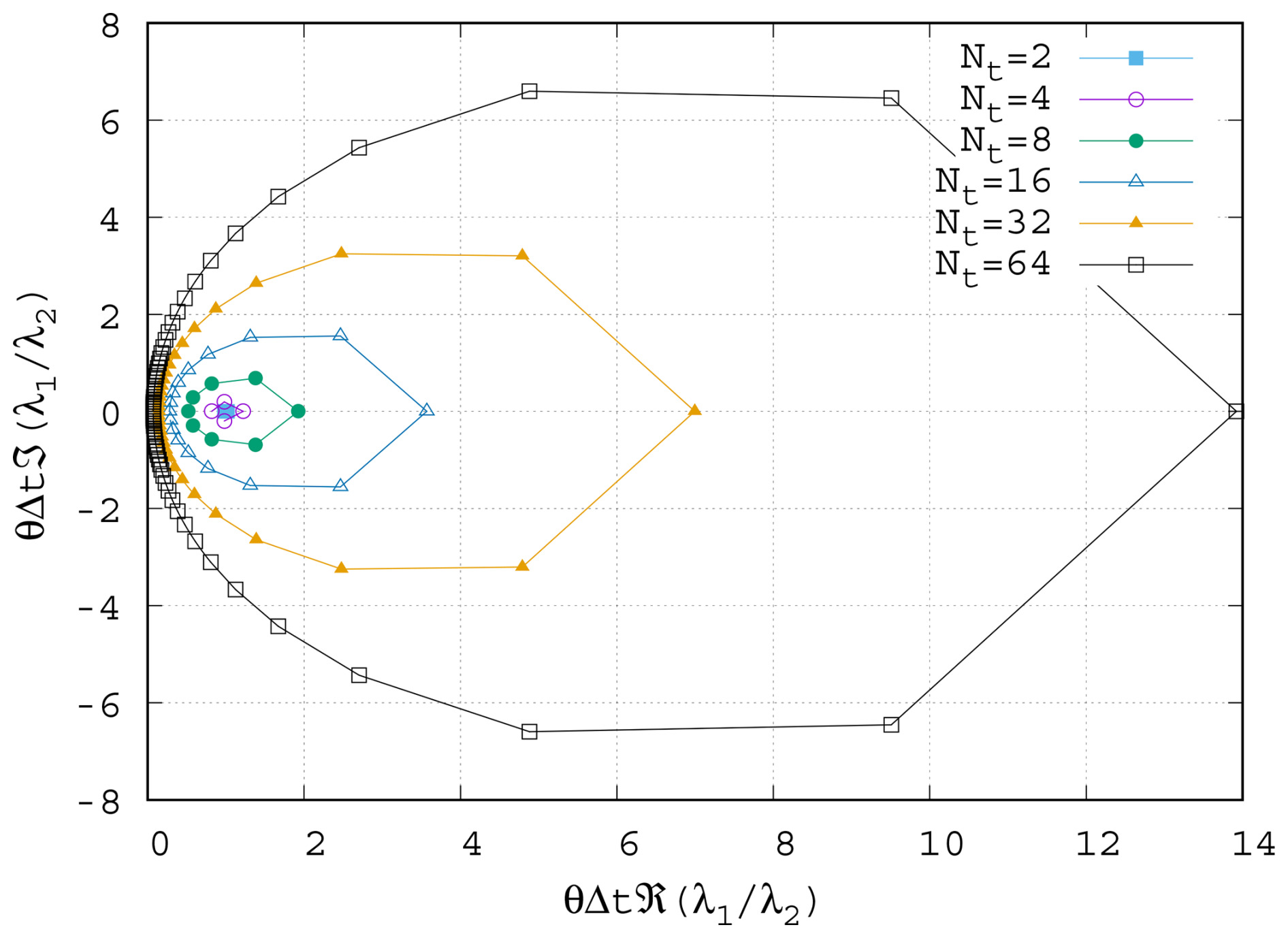
Figure 1 ${\mathit{\psi }}_j=({\mathit{\lambda }}_{\mathrm{1},j}/{\mathit{\lambda }}_{\mathrm{2},j})/(\mathrm{1}/(\mathrm{\Delta }t\mathit{\theta }\left)\right)$ in the complex plane for varying N_t with θ=0.5 and $\mathit{\alpha }={\mathrm{10}}^{-\mathrm{4}}$. As N_t increases, the ψ_j values for low frequencies cluster towards the imaginary axis.

Before moving on to consider nonlinear problems, we will briefly discuss the complex-valued block systems in Step 2 of the algorithm above. We compare these blocks to the implicit linear system $(M/\mathrm{\Delta }t+\mathit{\theta }K)$ in the serial-in-time method in Eq. (2). For consistent naming convention, we refer to the linear system from the serial-in-time method as the “real-valued block” contrasted with the “complex-valued blocks” in the circulant preconditioner. In each case we need to solve blocks of the form

$$\begin{array}{}\text{(15)}& \left({\displaystyle \frac{{\mathit{\beta }}_{\mathrm{1}}}{{\mathit{\beta }}_{\mathrm{2}}}}M+K\right)x={\displaystyle \frac{\mathrm{1}}{{\mathit{\beta }}_{\mathrm{2}}}}b,\end{array}$$

where (β₁,β₂) is $(\mathrm{1}/\mathrm{\Delta }t,\mathit{\theta })$ in the serial-in-time method and $({\mathit{\lambda }}_{\mathrm{1},j},{\mathit{\lambda }}_{\mathrm{2},j})$ in the parallel-in-time method, where λ_1,j and λ_2,j are the jth eigenvalue of C₁ and C₂ respectively. We have divided throughout by β₂ to make comparison easier. The ratio of the coefficient on the mass matrix M in the parallel-in-time method to the coefficient in the serial-in-time method is

$$\begin{array}{}\text{(16)}& {\mathit{\psi }}_j={\displaystyle \frac{{\mathit{\lambda }}_{\mathrm{1},j}/{\mathit{\lambda }}_{\mathrm{2},j}}{\mathrm{1}/\left(\mathrm{\Delta }t\mathit{\theta }\right)}}.\end{array}$$

Figure 1 shows ψ plotted in the complex plane for increasing N_t. When N_t is small, ψ_j is clustered around unity, and the blocks in the parallel-in-time method are almost identical to those in the serial-in-time method. However, as N_t increases, ψ_j spreads further from unity in all directions. The magnitude of ψ_j for high-frequency modes increases, with a real part ≥1, which is comparable to a small (albeit complex) time step and is usually a favourable regime for iterative solvers. On the other hand, the ψ_j for low-frequency modes cluster closer and closer to the imaginary axis as N_t increases. This resembles the case of a very large and mostly imaginary time step (and hence a large, imaginary, Courant number), which is challenging for many iterative methods.

2.2 Nonlinear problems

The method as presented so far is designed for linear problems with constant coefficients. However, many problems of interest are nonlinear in nature or have non-constant coefficients. In this section we will show the all-at-once system for nonlinear problems and show how the ParaDiag method can be applied to such problems. We consider PDEs of the form

$$\begin{array}{}\text{(17)}& M{\partial }_{t}u+f(u,t)=\mathrm{0},\end{array}$$

where the function$f(u,t):{\mathbb{R}}^{N_x}\times \mathbb{R}\to {\mathbb{R}}^{N_x}$ may be nonlinear. The discretisation of Eq. (17) with the implicit θ method is analogous to Eq. (2) with Kuⁿ replaced by f(uⁿ,tⁿ). The all-at-once system for the nonlinear PDE, analogous to Eq. (4), is

$$\begin{array}{}\text{(18)}& \left(B_{\mathrm{1}}\otimes M\right)\mathit{u}+\left(B_{\mathrm{2}}\otimes I_x\right)\mathbf{f}(\mathit{u}\mathbf{,}\mathit{t})=\stackrel{\mathrm{̃}}{\mathit{b}},\end{array}$$

where $\mathbf{f}(\mathit{u},\mathit{t}):{\mathbb{R}}^{N_t{N}_x}\times {\mathbb{R}}^{N_t}\to {\mathbb{R}}^{N_t{N}_x}$ is the concatenation of the function evaluations for the whole time series, which we show again for four time steps:

$$\begin{array}{}\text{(19)}& \mathbf{f}(\mathit{u},\mathit{t})=\left(\begin{array}{c}f(u^{\mathrm{1}},t^{\mathrm{1}})\\ f(u^{\mathrm{2}},t^{\mathrm{2}})\\ f(u^{\mathrm{3}},t^{\mathrm{3}})\\ f(u^{\mathrm{4}},t^{\mathrm{4}})\end{array}\right),\end{array}$$

where the vector of time values t is

$$\begin{array}{}\text{(20)}& \mathit{t}=\left(\begin{array}{c}{t}^{\mathrm{1}}\\ t^{\mathrm{2}}\\ t^{\mathrm{3}}\\ t^{\mathrm{4}}\end{array}\right).\end{array}$$

The right-hand side $\stackrel{\mathrm{̃}}{\mathit{b}}$ of Eq. (18) resembles Eq. (8) with Ku⁰ replaced by f(u⁰). This nonlinear system can be solved with a quasi-Newton method once a suitable Jacobian has been chosen. The exact Jacobian of Eq. (18) is

$$\begin{array}{}\text{(21)}& \mathbf{J}(\mathit{u},\mathit{t})=\left(B_{\mathrm{1}}\otimes M\right)+\left(B_{\mathrm{2}}\otimes I_x\right){\mathrm{\nabla }}_{\mathit{u}}\mathbf{f}(\mathit{u},\mathit{t}),\end{array}$$

where ${\mathrm{\nabla }}_{\mathit{u}}\mathit{f}(\mathit{u},\mathit{t})\in {\mathbb{R}}^{N_t{N}_x\times N_t{N}_x}$ is the derivative of f with respect to u and is a block-diagonal matrix with the nth diagonal block corresponding to the spatial Jacobian of f with respect to uⁿ, i.e. ${\mathrm{\nabla }}_{u}f(u^n,t^n)\in {\mathbb{R}}^{N_x\times N_x}$. Unlike K in the constant coefficient linear system in Eq. (4), the spatial Jacobian ∇_uf varies at each time step either through nonlinearity, time-dependent coefficients, or both. As such, Eq. (21) cannot be written solely as a sum of Kronecker products like the Jacobian in Eq. (4), and we cannot immediately apply the same α-circulant trick as before to construct a preconditioner. First, we must choose some constant-in-time value for the spatial Jacobian. Gander and Halpern (2017) proposed to average the spatial Jacobians over all time steps $\stackrel{\mathrm{‾}}{{\mathrm{\nabla }}_{u}f}={\sum }_{n=\mathrm{1}}^{N_t}{\mathrm{\nabla }}_{u}f(u^n,t^n)/N_t$. In our implementation, we use a constant-in-time reference state $\widehat{u}$ and reference time $\widehat{t}$ and evaluate the spatial Jacobian using these reference values (this choice is discussed further in Sect. 3.3). We also allow the preconditioner to be constructed from a different nonlinear function $\widehat{f}$; this allows for a variety of quasi-Newton methods. Using ${\mathrm{\nabla }}_u\widehat{f}(\widehat{u},\widehat{t})$, we can construct an α-circulant preconditioner according to

$$\begin{array}{}\text{(22)}& \mathbf{P}(\widehat{u},\widehat{t})=C_{\mathrm{1}}\otimes M+C_{\mathrm{2}}\otimes {\mathrm{\nabla }}_u\widehat{f}(\widehat{u},\widehat{t}).\end{array}$$

The preconditioner in Eq. (22) can be used with a quasi-Newton–Krylov method for Eq. (18). The preconditioner in Eq. (22) has two sources of error: the α-circulant block as in the linear case and now also the difference between ${\mathrm{\nabla }}_u\widehat{f}(\widehat{u},\widehat{t})$ and ∇_uf(uⁿ,tⁿ) at each step. For a fixed $\widehat{f}$, $\widehat{u}$, and $\widehat{t}$, we can define a function g which quantifies the “error” in the spatial Jacobian at a given t.

$$\begin{array}{}\text{(23)}& g(u;t)=f(u,t)-\left({\mathrm{\nabla }}_u\widehat{f}\left(\widehat{u},\widehat{t}\right)\right)u\end{array}$$

The Lipschitz constant of g with respect to u, over the time domain of interest, is the smallest κ such that

$$\begin{array}{}\text{(24)}& \Vert g(v;t)-g(w;t)\Vert \le \mathit{\kappa }\Vert v-w\Vert \forall t\in [\mathrm{0},T].\end{array}$$

By analogy to Picard iterations for the Dahlquist equation with an approximate circulant preconditioner, Čaklović (2023, Theorem 3.6 and Remark 3.8) estimates the convergence rate η of the quasi-Newton method as

$$\begin{array}{}\text{(25)}& \mathit{\eta }\sim {\displaystyle \frac{\mathit{\vartheta }\mathit{\kappa }{N}_t\mathrm{\Delta }t+\mathit{\alpha }}{\mathrm{1}-\mathit{\alpha }}},\end{array}$$

where N_tΔt=T is the duration of the time window, and ϑ is a constant that depends on the time integrator (Čaklović, 2023). This result can be understood as stating that the convergence rate deteriorates as the nonlinearity of the problem gets stronger (κ increases) or as the all-at-once system encompasses a longer time window (T=N_tΔt increases). The estimate implies that if α is small enough, then, for any moderate nonlinearity, the predominant error source will be the choice of reference state.

We now highlight the flexibility that expressing Eq. (18) as a preconditioned quasi-Newton–Krylov method provides. There are four main aspects, as follows.

1. At each Newton iteration, the Jacobian in Eq. (21) can be solved exactly (leading to a “true” Newton method) or inexactly (quasi-Newton). In the extreme case of the least exact Jacobian, the Jacobian is simply replaced by the preconditioner in Eq. (22), as in previous studies (Gander and Halpern, 2017; Gander and Wu, 2019; Čaklović, 2023; Wu and Zhou, 2021).

2. The nonlinear function $\widehat{f}$ used in the preconditioner in Eq. (22) does not need to be identical to the nonlinear function f in Eq. (18). The Jacobian in Eq. (21) has been written using f, but in general it could also be constructed from yet another function (not necessarily equal to either f or $\widehat{f}$). For example if Eq. (18) contains both linear and nonlinear terms, the Jacobian and/or preconditioner may be constructed solely from the linear terms, as in Čaklović (2023).

3. The Jacobian J(u,t) in Eq. (21) need not be linearised around the current Newton iterate u, but instead it could be linearised around some other time-varying state $\widehat{\mathit{u}}$, e.g. some reduced-order reconstruction of u.

4. Usually the reference state $\widehat{u}$ for the preconditioner $\mathbf{P}(\widehat{u},\widehat{t})$ in Eq. (22) is chosen to be the time-average state and is updated at every Newton iteration; however, any constant-in-time state may be used (e.g. the initial conditions). This may be favourable if $\widehat{u}$ does not change between Newton iterations, and a factorisation of ${\mathrm{\nabla }}_u\widehat{f}(\widehat{u},\widehat{t})$ may be reused across multiple iterations.

2.3 Performance model

In this section we present a simple performance model for ParaDiag. The purpose of the model is firstly to identify the factors determining the effectiveness of the method and secondly to help us later demonstrate that we have produced a reasonably performant implementation in asQ. The model extends those presented in Maday and Rønquist (2008) and Čaklović et al. (2021) by a more quantitative treatment of the block solve cost. In Maday and Rønquist (2008) it is assumed that the cost of the block solves in the all-at-once preconditioner is identical to the block solves in the serial-in-time method. In Čaklović et al. (2021) the costs are allowed to be different, but the difference is not quantified. Here we assume that an iterative Krylov method is used to solve both the real- and complex-valued blocks and that, because of the variations in ψ_j in Eq .(16), the number of iterations required is different for the blocks in the circulant preconditioner and in the serial-in-time method. In the numerical examples we will see that accounting for the difference in the number of block iterations is essential for accurately predicting performance. We assume perfect weak scaling in space for the block iterations: the time taken per Krylov iteration for the complex-valued blocks in Step 2 to apply the preconditioner is the same as the time taken per Krylov iteration for the real-valued blocks in the serial-in-time method so long as twice the number of processors is used for spatial parallelism.

We start with a simple performance model for the serial-in-time method for N_t time steps of the system in Eq. (17) with N_x degrees of freedom (DoFs) in space. Each time step is solved sequentially using Newton's method, requiring a certain number of (quasi-)Newton iterations per time step where, at each Newton iteration, the real-valued block $(M/\mathrm{\Delta }t+\mathit{\theta }{\mathrm{\nabla }}_{u}f)$ is solved (possibly inexactly) using a Krylov method. We assume that the block solves constitute the vast majority of the computational work in both the serial- and parallel-in-time methods and will revisit this assumption later. The cost of each time step is then proportional to the number of Krylov iterations k_s per solve of the real-valued block and to the number of times m_s the real-valued block must be solved per time step. For linear problems m_s=1 and for nonlinear problems, m_s is the number of Newton iterations. We assume that each Krylov iteration on the block requires work proportional to $N_x^q$, where the exponent q determines the scalability in space; for example a textbook multigrid method has q=1, and a sparse direct solve of a 2D finite element matrix has k_s=1 and $q=\mathrm{3}/\mathrm{2}$ (up to some upper limit on N_x). The cost of solving N_t time steps serial-in-time is therefore proportional to

$$\begin{array}{}\text{(26)}& W_{\mathrm{s}}\sim m_{\mathrm{s}}{k}_{\mathrm{s}}{N}_x^q{N}_t.\end{array}$$

The s subscript refers to “serial”(-in-time). If we parallelise only in space and assume weak scaling, then the number of processors is proportional to the number of spatial degrees of freedom, i.e. P_s∼N_x (this relation also holds once we have reached saturation when strong scaling). If the spatial parallelism weak scales perfectly with N_x, then the time taken to calculate the entire time series using the serial-in-time method is

$$\begin{array}{}\text{(27)}& T_{\mathrm{s}}\approx {\displaystyle \frac{W_{\mathrm{s}}}{P_{\mathrm{s}}}}\sim m_{\mathrm{s}}{k}_{\mathrm{s}}{N}_x^{q-\mathrm{1}}{N}_t,\end{array}$$

from which in can be seen that T_s is linear in N_t.

The nonlinear all-at-once system in Eq. (18) is solved using a (quasi-)Newton–Krylov method, shown in Algorithm 2. At each Newton iteration, this requires first evaluating the nonlinear residual of Eq. (18) (lines 3 and 8). Then, the update δu is calculated by solving (possibly inexactly) a linear system with the all-at-once Jacobian J in Eq. (21) using an iterative Krylov method, referred to as the outer Krylov method (line 5). Each outer Krylov iteration requires calculating both a matrix–vector multiplication for the action of J on a vector and the application of the circulant preconditioner P in Eq. (22). The preconditioner is applied using Algorithm 1, which in Step 2 requires solving (possibly inexactly) each complex-valued block using a separate Krylov method, referred to as the inner Krylov method.¹ The inner Krylov iterations may also be preconditioned, based on the structure of the blocks for the particular PDE being solved.

Algorithm 2 Newton–Krylov algorithm to solve the all-at-once system in Eq. (18) to a tolerance ntol. The Krylov method approximately solves Jδu=r, preconditioned with P, to a tolerance ktol. P is applied using Algorithm 1.

1:

Input: Initial solution guess u₀, Newton tolerance ntol, Krylov tolerance ktol

2:

k←0 {Newton iteration counter}

3:

r←nonlinear residual(u_k) {Residual evaluation Eq. (18)}

4:

while $\Vert \mathbf{r}\Vert <ntol$ {Newton iterations for Eq. (18)} do

5:

$\mathit{\delta }\mathbf{u}\leftarrow \text{Krylov}(\mathbf{r},\mathbf{J},\mathbf{P},ktol)$ {Newton update direction}

6:

${\mathbf{u}}_{k+\mathrm{1}}={\mathbf{u}}_k+\mathit{\delta }\mathbf{u}$

7:

$k\leftarrow k+\mathrm{1}$

8:

r←nonlinear residual(u_k)

9:

end while

10:

u←u_k

11:

return  u {All-at-once solution Eq. (7)}

Assuming that the block solves constitute the vast majority of the computational load, we estimate the total work required by starting from this inner level of the Newton–Krylov algorithm. If k_p inner Krylov iterations are required to solve each complex-valued block in Step 2 of Algorithm 1, and if we use the same solver as for the real-valued blocks so that the work per inner Krylov iteration is $N_x^q$, then the work for a single block solve is proportional to $k_{\mathrm{p}}{N}_x^q$. Each block is solved once per application of the circulant preconditioner, so the total work is the cost per block solve multiplied by the number of blocks N_t and by the total number of circulant preconditioner applications m_p. This m_p is the total over the entire Newton solve, i.e. the total number of outer Krylov iterations across all Newton iterations in Algorithm 2. (Note that for linear systems, where J reduces to A, m_p≠1 but is equal to the number of outer Krylov iterations to solve A). Finally, this gives the following estimate for the total computational work to solve Eq. (18):

$$\begin{array}{}\text{(28)}& W_{\mathrm{p}}\sim \mathrm{2}{m}_{\mathrm{p}}{k}_{\mathrm{p}}{N}_x^q{N}_t,\end{array}$$

where the p subscript refers to “parallel”(-in-time), and the factor of 2 accounts for the blocks being complex-valued.

We revisit the assumption that W_p is dominated by the complex-valued block solves. The main computational components of the ParaDiag method are the evaluation of the residual of Eq. (18), the action of the all-at-once Jacobian in Eq. (21), solving the complex-valued blocks in the circulant preconditioner, the collective communications for the space–time data transposes, and the (I)FFTs. In the numerical examples we will see that, in practice, the contributions to the runtime profile of the (I)FFTs and evaluating the residual are negligible, and the contribution of the Jacobian action is only a fraction of that of the block solves, so we do not include these operations in the performance model. This leaves just the computational work of the block solves, and the time taken for the space–time transpose communications in Steps 1 and 3.

The parallel-in-time method is parallelised across both time and space, giving

$$\begin{array}{}\text{(29)}& P_{\mathrm{p}}\sim \mathrm{2}{N}_x{N}_t.\end{array}$$

The factor of 2 ensures that the number of floating point numbers per processor in the complex-valued block solves is the same as in the real-valued block solves. The time taken to complete the calculation is then

$$\begin{array}{}\text{(30)}& T_{\mathrm{p}}\approx {\displaystyle \frac{W_{\mathrm{p}}}{P_{\mathrm{p}}}}+m_{\mathrm{p}}{T}_{\mathrm{c}}=m_{\mathrm{p}}\left(k_{\mathrm{p}}{N}_x^{q-\mathrm{1}}+T_{\mathrm{c}}\right),\end{array}$$

where T_c is the time taken for the collective communications in the space–time data transposes per preconditioner application. This leads to an estimate S of the speedup over the serial-in-time (but possibly parallel-in-space) method of

$$\begin{array}{}\text{(31)}& \begin{array}{rl}{\displaystyle \frac{T_{\mathrm{s}}}{T_{\mathrm{p}}}}\approx S& {\displaystyle }={\displaystyle \frac{m_{\mathrm{s}}{k}_{\mathrm{s}}{N}_x^{q-\mathrm{1}}{N}_t}{m_{\mathrm{p}}\left(k_{\mathrm{p}}{N}_x^{q-\mathrm{1}}+T_{\mathrm{c}}\right)}}\\ {\displaystyle }& {\displaystyle }=\left({\displaystyle \frac{N_t}{\mathit{\gamma }\mathit{\omega }}}\right){\displaystyle \frac{\mathrm{1}}{\mathrm{1}+T_{\mathrm{c}}/T_{\mathrm{b}}}},\end{array}\end{array}$$

where

$$\begin{array}{}\text{(32)}& \mathit{\gamma }={\displaystyle \frac{k_{\mathrm{p}}}{k_{\mathrm{s}}}},\mathit{\omega }={\displaystyle \frac{m_{\mathrm{p}}}{m_{\mathrm{s}}}},\text{ and }{T}_{\mathrm{b}}=k_{\mathrm{p}}{N}_x^{q-\mathrm{1}}.\end{array}$$

Here, γ quantifies how much more “difficult” the blocks in the circulant preconditioner are to solve than the blocks in the serial method, ω quantifies how much more “difficult” the all-at-once system is to solve than one time step of the serial method, and T_b is the time taken per block solve. If T_c≪T_b, then the speedup estimate simplifies to $N_t/\left(\mathit{\gamma }\mathit{\omega }\right)$ and depends solely on the “algorithmic scaling”, i.e. the dependence on N_t of the block and all-at-once system iteration counts. However, the speedup will suffer once T_c becomes non-negligible compared to T_b. Because both T_c and T_b are independent of m_p, we would expect this to happen only for larger N_t, independently of how effective the circulant preconditioner is.

From the speedup estimate in Eq. (31), we can estimate the parallel efficiency as

$$\begin{array}{}\text{(33)}& E={\displaystyle \frac{S}{P_{\mathrm{p}}/P_{\mathrm{s}}}}={\displaystyle \frac{S}{\mathrm{2}{N}_t}}=\left({\displaystyle \frac{\mathrm{1}}{\mathrm{2}\mathit{\gamma }\mathit{\omega }}}\right){\displaystyle \frac{\mathrm{1}}{\mathrm{1}+T_{\mathrm{c}}/T_{\mathrm{b}}}}.\end{array}$$

Note that using $P_{\mathrm{p}}/P_{\mathrm{s}}$ as the processor count means that Eq. (33) estimates the efficiency of the time-parallelism independently of the efficiency of the space parallelism, just as Eq. (31) estimates the speedup over the equivalent serial-in-time method independently of the space parallelism.

3 asQ library

In this section we introduce and describe asQ. First we state the aims of the library. Secondly, we take the reader through a simple example of solving the heat equation with asQ. Once the reader has a picture of the basic usage of asQ, we discuss how the library is structured to meet the stated aims. Next, we briefly describe the space–time Message Passing Interface (MPI) parallelism. Lastly, we describe the main classes in the library with reference to the mathematical objects from Sect. 2 that they represent.

asQ is open-source under the MIT licence and is available at https://github.com/firedrakeproject/asQ (last access: 14 July 2025). It can be installed by cloning or forking the repository and pip installing in a Firedrake virtual environment.² It is also installed in the Firedrake Docker container available on Docker Hub.

3.1 Library overview

A major difficulty in the development and adoption of parallel-in-time methods is their difficulty of implementation. Adapting an existing serial-in-time code to be parallel-in-time often requires major overhauls from the top level, and many parallel-in-time codes are written from the ground up as small codes or individual scripts for developing new methods. The simplest implementation is often to hard code a specific problem and solution method, which then necessitates significant additional effort to test new cases in the future. Once a promising method is found, it must be tested at scale on a parallel machine to confirm whether it actually achieves real speedups. However, efficiently parallelising a code can be time-consuming in itself and is a related but distinct skill set to developing a good numerical algorithm.

In light of these observations, we state the three aims of the asQ library for being a productive tool for developing ParaDiag methods.

• 1.

  It must be straightforward for a user to test out different problems – both equations sets and test cases.

• 2.

  It must be straightforward for a user to try different solution methods. We distinguish between two aspects:

  • a.

    the construction of the all-at-once systems, e.g. specifying the form of the all-at-once Jacobian or the state to linearise the circulant preconditioner around and

  • b.

    the linear/nonlinear solvers used, e.g. the Newton method used for the all-at-once system or the preconditioning used for the linear block systems.

• 3.

  The implementation must be efficient enough that a user can scale up to large-scale parallelism and get a realistic indication of the performance of the ParaDiag method.

Broadly, we attempt to fulfil these aims by building asQ on top of the Unified Form Language (UFL), Firedrake, and PETSc libraries and by following the design ethos of these libraries. The UFL (Alnæs et al., 2014) is a purely symbolic language for describing finite element forms, with no specification of how those forms are implemented or solved. UFL expressions can be symbolically differentiated, which allows for the automatic generation of Jacobians and many matrix-free methods. Firedrake is a Python library for the solution of finite element methods that takes UFL expressions and uses automatic code generation to compile high-performance C kernels for the forms. Firedrake integrates tightly with PETSc via petsc4py (Dalcin et al., 2011) for solving the resulting linear and nonlinear systems. PETSc provides a wide range of composable linear and nonlinear solvers that scale to massive parallelism (Lange et al., 2013; May et al., 2016), as well as mechanisms for creating new user-defined solver components, e.g. preconditioners. After the example script below we will discuss further how the three aims above are met.

We reinforce that asQ is not intended to be a generic ParaDiag library into which users can port their existing serial-in-time codes, as XBraid is for MGRIT or pySDC is for spectral deferred correction (SDC) and collocation methods. asQ requires a Firedrake installation and for the user to have some familiarity with basic Firedrake usage and to consider a modelling approach that is within the Firedrake paradigm (essentially a discretisation expressible in the domain-specific language UFL). In return for this restriction we gain all the previously mentioned benefits of Firedrake and PETSc for increasing developer productivity and computational performance. Restricting the scope to finite element methods means that a user does not need to implement spatial discretisations to experiment with temporal solution methods – this is in contrast to XBraid, pySDC, and pyParaDiag, which do not restrict the spatial discretisation at the cost of requiring user implementations. Additionally, we believe that for ParaDiag in particular it is important to have easy access to a wide range of linear solvers because the complex-valued coefficients on the block systems in Eq. (15) can impair the performance of iterative methods, so a range of strategies may have to be explored before finding a sufficiently efficient scheme. Contrast this with MGRIT or parareal, for example, where the inner solves are exactly the serial-in-time method, so existing solvers are often still optimal.

3.2 A heat equation example

The main components of asQ will be demonstrated through an example. We solve the heat equation over the domain Ω with boundary Γ:

$$\begin{array}{}\text{(34)}& {\displaystyle }{\partial }_{t}u-{\mathrm{\nabla }}^{\mathrm{2}}u=\mathrm{0}& {\displaystyle }\text{ in }\mathrm{\Omega },\text{(35)}& {\displaystyle }n\cdot \mathrm{\nabla }u=\mathrm{0}& {\displaystyle }\text{ on }{\mathrm{\Gamma }}_{\mathrm{N}},\text{(36)}& {\displaystyle }u=\mathrm{0}& {\displaystyle }\text{ on }{\mathrm{\Gamma }}_{\mathrm{D}},\end{array}$$

where n is the normal to the boundary, Γ_N is the section of the boundary with zero Neumann boundary conditions, Γ_D is the section of the boundary with zero Dirichlet boundary conditions, and ${\mathrm{\Gamma }}_{\mathrm{N}}\cup {\mathrm{\Gamma }}_{\mathrm{D}}=\mathrm{\Gamma }$. Equation (34) will be discretised with a standard continuous Galerkin method in space. If V is the space of piecewise linear functions over the mesh, and V₀ is the space of functions in V which are 0 on Γ_D, the solution u∈V₀ is the solution of the weak form:

$$\begin{array}{}\text{(37)}& \underset{\mathrm{\Omega }}{\int }\left(v{\partial }_{t}u+\mathrm{\nabla }u\cdot \mathrm{\nabla }v\right)\text{d}\mathit{x}=\mathrm{0}\forall v\in V_{\mathrm{0}}.\end{array}$$

The Neumann boundary conditions are enforced weakly by removing the corresponding surface integral, and the Dirichlet conditions are enforced strongly by restricting the solution to V₀.

We will set up and solve an all-at-once system for the backward Euler method for eight time steps distributed over four spatial communicators. The code for this example is shown in Listing 1 and is available in the heat.py script in Hope-Collins et al. (2024b).

The first part of the script will import Firedrake and asQ and set up the space–time parallel partition. asQ distributes the time series over multiple processors in time, and each time step may also be distributed in space. Firedrake's Ensemble class manages this distribution by setting up a tensor product P_x×P_t of MPI communicators for space and time parallelism (described in more detail later and illustrated in Fig. 2). The time parallelism is determined by the list time_partition on line 4. Here we request four processors in time, each holding two time steps for a total time series of eight time steps. We refer to all time steps on a single partition in time as a “slice” of the time series; here, we have four slices of two time steps each.

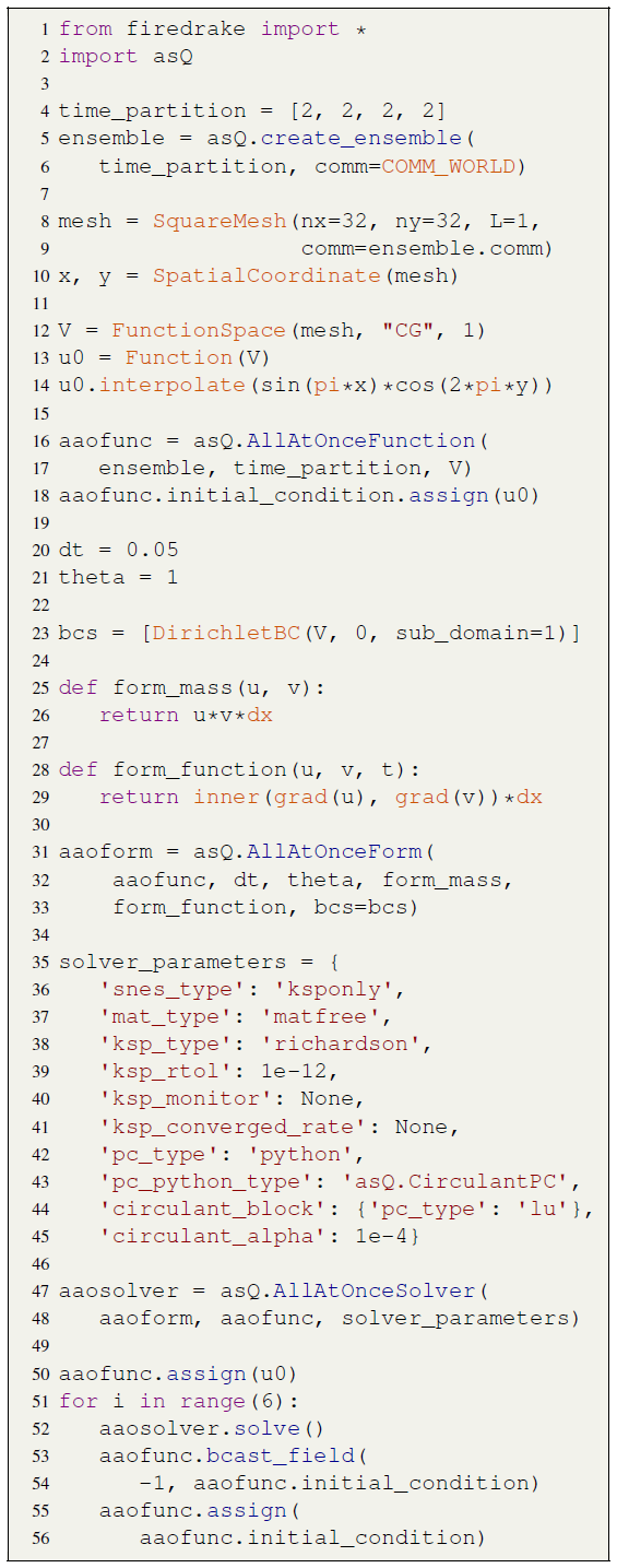
Listing 1 Code for solving the heat equation with ParaDiag (available in Hope-Collins et al., 2024b). asQ and Firedrake components are highlighted in blue and orange respectively.

We do not need to provide the spatial partition when we create the Ensemble on line 5 because the total MPI ranks will automatically be distributed evenly in time. For example if the script is run with four MPI ranks, then each spatial communicator will have a single rank, but if the script is run with eight MPI ranks, then each spatial communicator will have two MPI ranks.

On line 8 we define the mesh for a square domain $(x,y)\in \mathrm{\Omega }=(\mathrm{0},\mathrm{1})\times (\mathrm{0},\mathrm{1})$ defined on the local spatial communicator ensemble.comm. The linear continuous Galerkin ("CG") function space V for a single time step is represented by the Firedrake FunctionSpace on line 12 and is used to create a Firedrake Function holding the initial conditions u₀=sin(πx)cos(2πy).

Now we build the all-at-once system using asQ, starting with an AllAtOnceFunction on line 16. This class represents Eq. (7), a time series of finite element functions in V distributed in time over an Ensemble. In an AllAtOnceFunction each spatial communicator holds a slice of one or more time steps of the time series, in this example two time steps per communicator.

Next we need to define the all-at-once system itself. To represent the finite element form in Eq. (4) or Eq. (18) over the time series aaofunc, we use an AllAtOnceForm. Building this requires the time step Δt, the implicit parameter θ, the boundary conditions, and a way of describing the mass matrix M and the function f(u,t) (which for linear equations is just Ku). This is shown between lines 20 and 33. The time step Δt=0.05 gives a Courant number of around 13, and θ=1 gives the implicit Euler time-integration method. The Python functions form_mass and form_function each take in a function u and a test function v in V and return the UFL form for the mass matrix M and f(u,t) respectively. asQ uses these two Python functions to generate all of the necessary finite element forms for the all-at-once system in Eq. (18), the Jacobian in Eq. (21), and the circulant preconditioner in Eq. (22), while the user need only define them for the semi-discrete form of a single time step. The boundary conditions for a single time step are passed to the AllAtOnceForm in bcs and are applied to all time steps. For Eq. (36) we set Γ_D to be the left boundary x=0 by passing the subdomain=1 argument to the DirichletBC, and for Eq. (35) Firedrake defaults to zero Neumann boundary conditions on all other boundaries. Given V and a set of Dirichlet boundary conditions, Firedrake will automatically create the restricted space V₀. The initial conditions defined earlier conform to these boundary conditions.

We next need to specify how we solve for the solution of aaoform. In PETSc, linear and nonlinear solvers are specified using dictionaries of solver parameter options, here shown on lines 35 to 45. Nonlinear problems are solved using a SNES (Scalable Nonlinear Equations Solver), and linear problems are solved using a KSP (Krylov SPace method), which is preconditioned by a PC. Starting with the SNES, our problem is linear, so we use 'snes_type': 'ksponly' to perform one Newton iteration and then return the result. Assembling the entire space–time matrix would be very expensive and is unnecessary for ParaDiag, so asQ implements the Jacobian matrix-free, specified by the 'mat_type': 'matfree' option. We select the Richardson iterative method and require a drop in the residual of 12 orders of magnitude. The ksp_monitor and ksp_converged_rate options tell PETSc to print the residual at each Krylov iteration and the contraction rate upon convergence respectively. The Richardson iteration is preconditioned with the corresponding block circulant ParaDiag matrix, which is provided by asQ as a Python type preconditioner CirculantPC with the circulant parameter $\mathit{\alpha }={\mathrm{10}}^{-\mathrm{4}}$. Lastly, we need to specify how to solve the blocks in the preconditioner after the diagonalisation. The composability of PETSc solvers means that to specify the block solver we simply provide another dictionary of options with the 'circulant_block' key. The block solver here is just a direct LU factorisation but could be any other Firedrake or PETSc solver configuration.

The tight integration of Firedrake and asQ with PETSc means that a wide range of solution strategies are available through the dictionary of options. For example, we can change the Krylov method for the all-at-once system simply by changing the 'ksp_type' option. Rather than a direct method, an iterative method could be used for the block solves by changing the options in the circulant_block dictionary. Options can also be passed from the command line, in which case zero code changes are required to experiment with different solution methods.

The last all-at-once object we need to create is an AllAtOnceSolver on line 47, which solves aaoform for aaofunc using the specified solver parameters. If we want to solve for, say, a total of 48 time steps, then, for an all-at-once system of size N_t=8, we need to solve six windows of 8 time steps each, where the final time step of each window is used as the initial condition for the next window, shown on lines 51 to 56. After each window solve, we use the final time step as the initial condition for the next window. To achieve this, aaofunc.bcast_field(i, uout) on line 53 wraps MPI_Bcast to broadcast time step i across the temporal communicators so that all spatial communicators now hold a copy of time step i in uout (in this example, i is the Pythonic −1 for the last element, and uout is the initial_condition). After broadcasting the new initial conditions, every time step in aaofunc is then assigned the value of the new initial condition as the initial guess of the next solve. We have been able to set up and solve a problem parallel in time (and possibly parallel in space) in 56 lines of code.

We now return to the three requirements stated in the library overview and discuss how asQ attempts to meet each one.

• 1.

  Straightforward to test different problems. This requirement is met by only requiring the user to provide UFL expressions for the mass matrix M and the function f(u,t): a Firedrake FunctionSpace for a single time step and a Firedrake Function for the initial conditions. These are all components that a user would already have, or would need anyway, to implement the corresponding serial-in-time method. From these components asQ can generate the UFL for the different all-at-once system components, which it then hands to Firedrake to evaluate numerically. Changing to a different problem simply requires changing one or more of the UFL expressions, the function space, or the initial conditions.

• 2.

  Straightforward to test different solution methods.

  • a.

    Requirement 2a is met by allowing users to optionally pass additional UFL expressions (form_function) for constructing the different all-at-once system components (see the AllAtOnceSolver, CirculantPC, and AuxiliaryBlockPC descriptions below).

  • b.

    Requirement 2b is met through the use of PETSc's solver options interface. Changing between many different methods is as simple as changing some options strings. For more advanced users, novel methods can be written as bespoke petsc4py Python PCs. The use of UFL means that symbolic information is retained all the way down to the block systems, so solution methods that rely on certain structure can be applied without issue, for example Schur factorisations or additive Schwarz methods defined on topological entities.

• 3.

  Efficient parallel implementation. This requirement involves both spatial and temporal parallelism. The spatial parallelism is entirely provided by Firedrake and PETSc. The temporal parallelism is implemented using a mixture of PETSc objects defined over the global communicator, and mpi4py calls via the Firedrake Ensemble or via the mpi4py-fftw library (Dalcin and Fang, 2021). The temporal parallelism is discussed in more depth in Sect. 3.3 and is profiled in the examples in Sect. 4.

3.3 Space–time parallelism

As stated previously, time parallelism is only used once space parallelism is saturated due to the typically lower parallel efficiency. This means that any practical implementation of parallel-in-time methods must be space–time parallel. In terms of evaluating performance, full space–time parallelism is especially important for ParaDiag methods due to the need for all-to-all communication patterns, which can be significantly affected by network congestion.

The three steps in applying the block circulant preconditioner require two distinct data access patterns. The (I)FFTs in Steps 1 and 3 require values at a particular spatial degree of freedom (DoF) at all N_t time steps/frequencies, whereas the block solves in Step 2 require values for all spatial DoFs at a particular frequency. The data layout in asQ places a single slice of the time series on each spatial communicator. The slice length is assumed to be small and is usually just one, i.e. a single time step per spatial communicator, to maximise time parallelism during Step 2. This layout minimises the number of ranks per spatial communicator, hence reducing the overhead of spatial halo swaps during the block solve. However, parallel FFTs are not efficient with so few values per processor. Instead of using a parallel FFT, the space–time data are transposed so that each rank holds the entire time series for a smaller number of spatial DoFs. Each rank can then apply a serial FFT at each spatial DoF. After the transform the data are transposed back to their original layout. These transposes require all-to-all communication rounds, which are carried out over each partition of the mesh separately, so we have P_x∼𝒪(N_x) all-to-all communications involving P_t∼𝒪(N_t) processors each, instead of a single all-to-all communication involving all P_tP_x processors. asQ currently uses the mpi4py-fftw library for these communications, which implements the transposes using MPI_Alltoallw and MPI derived data types.

Collective communication patterns, particularly Alltoall and its variants, do not scale well for large core counts compared to the point-to-point communications typical required for spatial parallelism. There are two common implementations of Alltoall in MPI: pairwise and Bruck (Netterville et al., 2022). The pairwise algorithm minimises the total communication volume but has communication complexity 𝒪(P). The Bruck algorithm has communication complexity 𝒪(log P) at the expense of a higher total communication volume, so it is only more efficient than the pairwise algorithm for latency bound communications (i.e. small message sizes). MPI implementations usually select which algorithm to use at runtime based on a variety of factors, primarily the number of processors in the communicator and the message size. The typical message size for ParaDiag is above the usual thresholds for the Bruck algorithm to be used. Therefore, we expect the communication time T_c in our performance model above to scale with 𝒪(P_t) and become a limiting factor on the parallel scaling for large N_t. It is worth noting that, although to a first approximation T_c should depend on P_t but not P_x for constant DoFs/core, in practice network congestion may cause T_c to increase with P_x even if P_t is fixed.

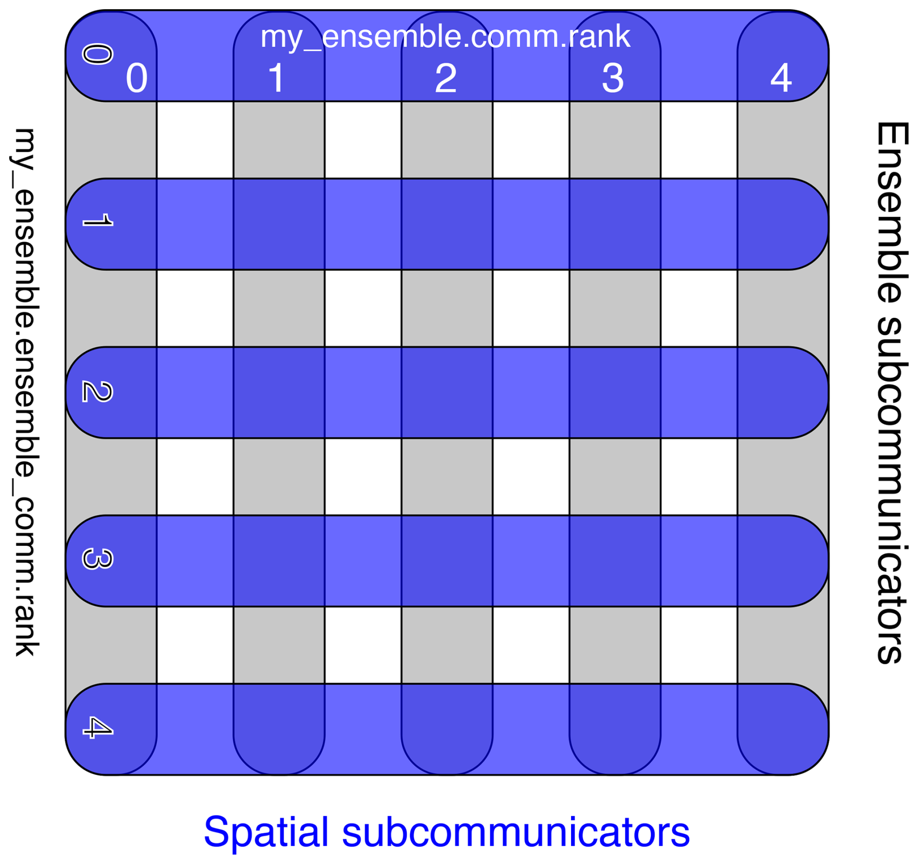
Figure 2 Space–time parallelism using Firedrake's Ensemble class. ensemble.comm.size is P_x=5, and ensemble.ensemble_comm.size is P_t=5. The dark-blue horizontal lines each represent a spatial communicator Ensemble.comm over which a mesh is partitioned. Every spatial communicator has the same number of ranks and the same mesh partitioning. The grey vertical lines represent communicators in time, Ensemble.ensemble_comm. These communicators are responsible for connecting the ranks on each spatial communicator with the same section of the mesh partition.

The space–time parallelism in asQ is implemented using Firedrake's Ensemble class, which splits a global communicator (usually COMM_WORLD) into a Cartesian product of spatial and temporal communicators. The resulting layout of communicators in the Ensemble is shown in Fig. 2. Firedrake objects for each time step are defined on each spatial communicator, and PETSc objects and asQ objects for the all-at-once system are defined over the global space–time communicator. The Ensemble provides wrappers around mpi4py calls for sending Firedrake Function objects between spatial communicators over the temporal communicators. The mpi4py-fftw library is used for space–time transposes separately across each temporal communicator. The spatial parallelism required is already fully abstracted away by Firedrake, so asQ need only implement the temporal parallelism on top of this. The Ensemble splits the global communicator such that each spatial communicator has a group of consecutive cores, which minimises the amount of off-node communication needed during the block solves. This is important if we assume that the space parallelism will already be at the strong scaling limit before time parallelism is used. We experimented briefly with grouping the ranks in each temporal communicator consecutively, but the performance was either unchanged or reduced in all cases that we tried compared to grouping the ranks in each spatial communicators.

As stated earlier, in asQ we construct the circulant preconditioner from the spatial Jacobian of a constant reference state (usually the time-averaged state), rather than the time average of the spatial Jacobians. The time average of the spatial Jacobian is optimal in the L2 norm, but using the reference state has two advantages. First, the communication volume of averaging the state is smaller than averaging the Jacobians. For scalar PDEs or low-order methods the difference is minor, but for systems of PDEs or high-order methods the difference can be substantial. Second, explicitly assembling the Jacobian prevents the use of matrix-free methods provided by Firedrake and PETSc for the block solves. Matrix-free methods have lower memory requirements than assembled methods, which is important for finite element methods because they are usually memory-bound. The matrix-free implementation in Firedrake (Kirby and Mitchell, 2018) also enables the use of block preconditioning techniques such as Schur factorisation by retaining symbolic information that is lost when assembling a matrix numerically. We also note that for quadratic nonlinearities (such as in the shallow water equations in primal form) the Jacobian of the average and the average of the Jacobian are identical. However, for cubic or higher nonlinearities (such as the compressible Euler equations in conservative form) the two forms are not identical.

3.4 asQ components

Now that we have seen an example of the basic usage of asQ, we give a more detailed description of each component of the library, with reference to which mathematical objects described in Sect. 2 they represent. First the components of the all-at-once system are described, then a variety of Python type PETSc preconditioners for both the all-at-once system and the blocks, and then the submodule responsible for the complex-valued block solves in the circulant preconditioner. There are a number of other components implemented in asQ, but these are not required for the numerical examples later, so they are omitted here (see Appendix C for a description of some of these components).

AllAtOnceFunction

The AllAtOnceFunction is a time series of finite element functions distributed over an Ensemble representing the vector u in Eq. (7) plus an initial condition. Each ensemble member holds a slice of the time series of one or more time steps, and time step i can be accessed on its local spatial communicator as a Firedrake Function using aaofunc[i]. Evaluation of the θ-method residual in Eq. (2) at a time step uⁿ⁺¹ requires the solution at the previous time step uⁿ, so the AllAtOnceFunction holds time halos on each spatial communicator for the last time step on the previous slice. Some other useful operations are also defined, such as calculating the time average, linear vector space operations (e.g. axpy), and broadcasting particular time steps to all slices (bcast_field). Internally, a PETSc Vec is created for the entire space–time solution to interface with PETSc solvers.

AllAtOnceCofunction

In addition to functions in the primal space V, it is also useful to have a representation of cofunctions in the dual function space V^*. asQ provides this dual object as an AllAtOnceCofunction, which represents a time series of the dual space V^*. Cofunctions are used when assembling residuals of Eq. (4) or Eq. (18) over the time series and providing the right-hand side (the constant part) of linear or nonlinear systems. Both AllAtOnceFunction and AllAtOnceCofunction have a riesz_representation method for converting between the two spaces.

AllAtOnceForm

The AllAtOnceForm holds the finite element form for the all-at-once system Eq. (18) and is primarily responsible for assembling the residual of this form to be used by PETSc. It holds the Δt, θ, form_mass, form_function, and boundary conditions which are used for constructing the Jacobian and preconditioners. The contribution of the initial conditions to the right-hand side $\stackrel{\mathrm{̃}}{\mathit{b}}$ is automatically included in the system. After updating the time halos in the AllAtOnceFunction, assembly of the residual can be calculated in parallel across all slices. The AllAtOnceForm will also accept an α parameter to introduce the circulant approximation at the PDE level, such as required for the waveform relaxation iterative method of Gander and Wu (2019), which uses the modified initial condition $u^k\left(\mathrm{0}\right)=u_{\mathrm{0}}+\mathit{\alpha }\left(u^k\right(T)-u^{k-\mathrm{1}}(T\left)\right)$.

AllAtOnceJacobian

The AllAtOnceJacobian represents the action of the Jacobian in Eq. (21) of an AllAtOnceForm on an all-at-once function. This class is rarely created explicitly by the user, but it is instead created automatically by the AllAtOnceSolver or LinearSolver classes described below and used to create a PETSc Mat (matrix) for the matrix–vector multiplications required for Krylov methods. As for assembly of the AllAtOnceForm, calculating the action of the AllAtOnceJacobian is parallel across all slices after the time halos are updated. The automatic differentiation provided by UFL and Firedrake means that the action of the Jacobian is computed matrix-free, removing any need to ever explicitly construct the entire space–time matrix. For a quasi-Newton method the Jacobian need not be linearised around the solution at the current iteration. The AllAtOnceJacobian has a single PETSc option for specifying alternate states to linearise around, including the time average, the initial conditions, or a completely user-defined state.

AllAtOnceSolver

The AllAtOnceSolver is responsible for setting up and managing the PETSc SNES for the all-at-once system defined by an AllAtOnceForm using a given dictionary of solver options. The nonlinear residual is evaluated using the AllAtOnceForm, and an AllAtOnceJacobian is automatically created. By default this Jacobian is constructed from the AllAtOnceForm being solved, but AllAtOnceSolver also accepts an optional argument for a different AllAtOnceForm to construct the Jacobian from, for example one where some of the terms have been dropped or simplified. Just like Firedrake solver objects, AllAtOnceSolver accepts an appctx dictionary containing any objects required by the solver which cannot go into a dictionary of options (i.e. not strings or numbers). For example for CirculantPC this could include an alternative form_function for $\widehat{f}$ or a Firedrake Function for $\widehat{u}$ in Eq. (22).

Callbacks can also be provided to the AllAtOnceSolver to be called before and after assembling the residual and the Jacobian, similar to the callbacks in Firedrake's NonlinearVariationalSolver. There are no restrictions on what these callbacks are allowed to do, but potential uses include updating solution-dependent parameters before each residual evaluation and manually setting the state around which to linearise the AllAtOnceJacobian.

Paradiag

In most cases, users will want to follow a very similar workflow to that in the example above: setting up a Firedrake mesh and function space, building the various components of the all-at-once system, and then solving one or more windows of the time series. To simplify this, asQ provides a convenience class Paradiag to handle this case. A Paradiag object is created with the following arguments:

paradiag = Paradiag(
    ensemble=ensemble,
    form_mass=form_mass,
    form_function=form_function,
    ics=u0, dt=dt, theta=theta,
    time_partition=time_partition,
    solver_parameters=solver_parameters),

creating all the necessary all-at-once objects from these arguments. The windowing loop in the last snippet of the example above is also automated and can be replaced by

paradiag.solve(nwindows=6).

The solution is then available in paradiag.aaofunc, and the other all-at-once objects are similarly available. Callbacks can be provided to be called before and after each window solve, e.g. for writing output or collecting diagnostics.

SerialMiniApp

The SerialMiniApp is a small convenience class for setting up a serial-in-time solver for the implicit θ method and takes most of the same arguments as the Paradiag class.

serial_solver = SerialMiniApp(
   dt, theta, u0,
   form_mass, form_function,
   solver_parameters)

The consistency in the interface means that, once the user is satisfied with the performance of the serial-in-time method, setting up the parallel-in-time method is straightforward, with the only new requirements being the solver options and the description of the time parallelism (ensemble and time partition). Importantly, this also makes ensuring fair performance comparisons easier. In Sect. 4, all serial-in-time results are obtained using the SerialMiniApp class.

CirculantPC

The block α-circulant matrix in Eq. (22) is implemented as a Python type petsc4py preconditioner, which allows it to be applied matrix-free. By default the preconditioner is constructed using the same Δt, θ, form_mass, and form_function as the AllAtOnceJacobian and linearising the blocks around the time average $\widehat{u}$. However, alternatives for all of these can be set via the PETSc options and the appctx. For example, an alternate $\widehat{f}$ can be passed in through the appctx, and $\widehat{u}$ could be chosen as the initial conditions via the PETSc options. Additional solver options can also be set for the blocks, as shown in the example above. The implementation of the complex-valued linear system used for the blocks can also be selected via the PETSc options: more detail on this below.

AuxiliaryRealBlockPC and AuxiliaryComplexBlockPC

These two classes are Python preconditioners for a single real- or complex-valued block respectively, constructed from an “auxiliary operator”, i.e. from a different finite element form than the one used to construct the block. These are implemented by subclassing Firedrake's AuxiliaryOperatorPC. Examples of when preconditioning the blocks with a different operator may be of interest include preconditioning the nonlinear shallow water equations with the linear shallow water equations or preconditioning a variable diffusion heat equation with the constant diffusion heat equation. This preconditioner can be supplied with any combination of alternative values for form_mass, form_function, boundary conditions, (Δt,θ) or (λ₁,λ₂) as appropriate, and $(\widehat{u},\widehat{t})$, as well as PETSc options for how to solve the matrix resulting from the auxiliary operator.

complex_proxy

When PETSc is compiled, a scalar type must be selected (e.g. double-precision float, single-precision complex), and then only this scalar type is available. asQ uses PETSc compiled with a real-valued scalar because complex scalars would double the required memory access when carrying out real-valued parts of the computation, and not all of Firedrake's preconditioning methods are available in complex mode yet (notably geometric multigrid). However, this means that the complex-valued linear systems in the blocks of the CirculantPC must be manually constructed. The complex_proxy module does this by writing the linear system λAx=b with complex number $\mathit{\lambda }={\mathit{\lambda }}_r+i{\mathit{\lambda }}_i$, complex vectors $x=x_r+i{x}_i$ and $b=b_r+i{b}_i$, and real matrix A as

$$\begin{array}{}\text{(38)}& \left(\begin{array}{cc}{\mathit{\lambda }}_{r}A& -{\mathit{\lambda }}_{i}A\\ {\mathit{\lambda }}_{i}A& {\mathit{\lambda }}_{r}A\end{array}\right)\left(\begin{array}{c}{x}_r\\ x_i\end{array}\right)=\left(\begin{array}{c}{b}_r\\ b_i\end{array}\right).\end{array}$$

Two versions of complex_proxy are available, both having the same API but different implementations. One implements the complex function space as a two-component Firedrake VectorFunctionSpace and one which implements the complex function space as a two-component Firedrake MixedFunctionSpace. The VectorFunctionSpace implementation is the default because for many block preconditioning methods it acts more like a true complex-valued implementation. The complex_proxy submodule API will not be detailed here, but example scripts are available in the asQ repository demonstrating its use for testing block preconditioning strategies without having to set up an entire all-at-once system.

4 Numerical examples

We now present a set of numerical examples of increasing complexity in order to demonstrate two points, firstly that asQ is a correct and efficient implementation of the ParaDiag method and secondly that the ParaDiag method is capable of delivering speedups on relevant linear and nonlinear test cases from the literature. The correctness of asQ will be demonstrated by verifying the convergence rate in Eq. (14) from Sect. 2.1, and the efficiency of the implementation will be demonstrated by comparing actual wall-clock speedups to the performance model of Sect. 2.3.

In the current article we are interested only in speedup over the equivalent serial-in-time method: can ParaDiag accelerate the calculation of the solution to the implicit-θ method? We are not considering here the question of whether ParaDiag can beat the best of some set of serial-in-time methods (e.g. on error vs. wall-clock time). This question is the topic of a later publication.

The situation we consider is that we want a solution over a time interval of length T, which, for reasonable values of Δt, requires a large number of time steps $N_T=T/\mathrm{\Delta }t$. However, ParaDiag may be more efficient for all-at-once systems with N_t<N_T, so we split the time series of N_T time steps into N_w windows of $N_t=N_T/N_{\mathrm{w}}$ time steps each. We then use ParaDiag to solve the all-at-once system for each window in turn, using the last time step of each window as the initial condition for the next window.

For linear constant-coefficient equations, for a given α the number of iterations required to solve each window is constant, so if both α α and N_t are fixed, then the time taken to solve each window is essentially constant. Likewise, in the serial-in-time method the time taken per time step is essentially constant. This means that we can solve a single window of a given α and N_t, or a single time step serial-in-time, and extrapolate the time taken to solve all N_T time steps. In practice, network congestion and other hardware factors may affect the time taken, so in the linear examples below we actually solve five windows for each α and N_t combination and average the time taken – although we note that there was very little variation. For the nonlinear equations, both the serial- and parallel-in-time methods may require a different number of iterations per time step or window as the nonlinearity in the local solution evolves. For the nonlinear examples we calculate all N_T time steps for both serial-in-time and parallel-in-time methods and use the total time taken.

In the performance model in Eq. (31) it is assumed that, once spatial parallelism is saturated, the number of cores is proportional to the number of time steps in the all-at-once system N_t. We have not found a situation in which there is a speedup advantage to having more time steps than cores by having multiple time steps per time slice. Therefore in all examples we keep the DoFs/core constant when varying N_t or N_x, which, when combined with the framing of scaling in terms of resolution and wall-clock time, leads to the following strong- and weak-scaling interpretations. For strong scaling in time, Δt and N_T are fixed, and we attempt to decrease the total wall-clock time by increasing N_t and decreasing N_w. Although the number of DoFs being computed at any one time is increasing, with DoFs/core fixed (as it would be for traditional weak scaling in space), we call this strong scaling because the resolution is fixed. For weak scaling in time, Δt is decreased and N_T is increased proportionally such that the final time T remains the same. We attempt to keep the wall-clock time fixed by keeping N_w fixed but increasing N_t so that we can use more cores. Usually – but not necessarily – Δx is decreased proportionally to Δt, in which case the number of cores used for spatial parallelism will also increase to keep the DoFs/core constant.

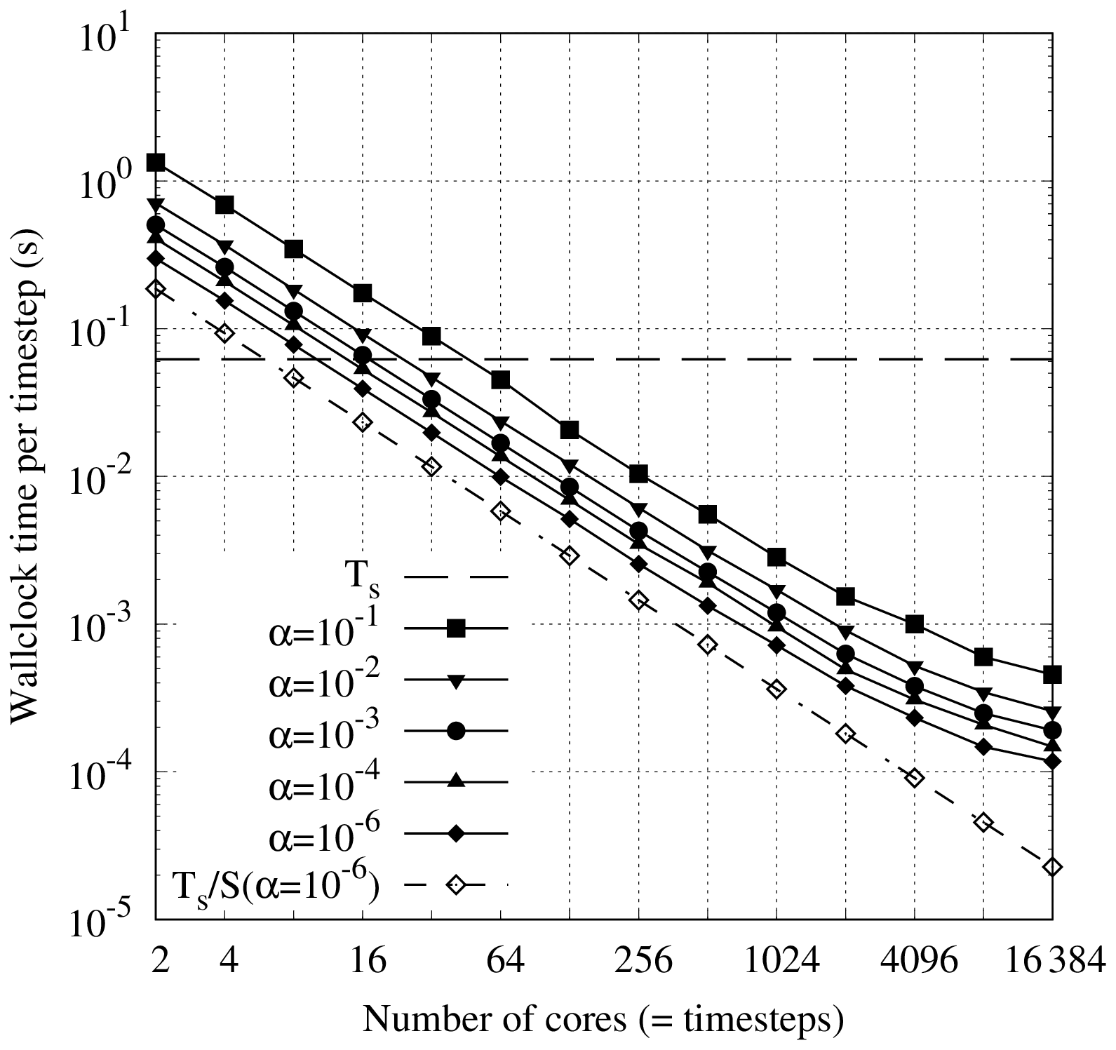
Figure 3 Strong scaling in time of the linear scalar advection equation test case with N_x=128² and σ=0.8 is demonstrated by measured wall-clock times per time step ($T_{\mathrm{p}}/N_t$) for varying N_t and α. The wall-clock time for the serial-in-time method is plotted as the horizontal line T_s. The prediction of the performance model $T_{\mathrm{s}}/S$ in Eq. (31) is shown for $\mathit{\alpha }={\mathrm{10}}^{-\mathrm{6}}$ using the measured T_s and $S=N_t/\left(\mathrm{2}(m_{\mathrm{p}}+\mathrm{1})\right)$ (assuming T_c=0). Maximum speedup of 528 achieved with $\mathit{\alpha }={\mathrm{10}}^{-\mathrm{6}}$ and N_t=16384.

All results presented here were obtained on the ARCHER2 HPE Cray supercomputer at the EPCC (Beckett et al., 2024) using a Singularity container with asQ, Firedrake, and PETSc installed. ARCHER2 consists of 5860 nodes, each with 2 AMD EPYC 7742 CPUs with 64 cores per CPU for a total of 128 cores per node. The nodes are connected with an HPE Slingshot network. The EPYC 7742 CPUs have a deep memory hierarchy, with the lowest level of shared memory being a 16 MB L3 cache shared between four cores. During preliminary testing we found that, due to the memory-bound nature of finite element computation, the best performance was obtained by underfilling each node by allocating fewer than four cores per L3 cache. For the examples using the shallow water equations and the compressible Euler equations, we use 2 cores per L3 cache, giving a maximum of 64 cores per node. For the advection equation example, using a single core per L3 cache gave the best scaling due to the small size of the spatial domain and the use of LU for the block solves, giving a maximum of 32 cores per node. For all cases we have only one time step per Ensemble member to maximise the available time parallelism. Unless otherwise stated, we use twice as many cores per time step in the parallel-in-time method as in the serial-in-time method to account for the complex-valued nature of the blocks in the circulant preconditioner.

The software used to generate the results in this section is available via Zenodo: Hope-Collins et al. (2024b) for the Python scripts; Hope-Collins et al. (2024a) for the Singularity image containing a build of PETSc, Firedrake, and asQ; Hope-Collins et al. (2025) for the asQ library version; and firedrake zenodo (2024) for the versioned Firedrake and PETSc libraries and their dependencies. The Python scripts may be run with the Singularity container without requiring a separate Firedrake installation. Details on the finite element forms used for each example can be found in Appendix B.

4.1 Advection equation

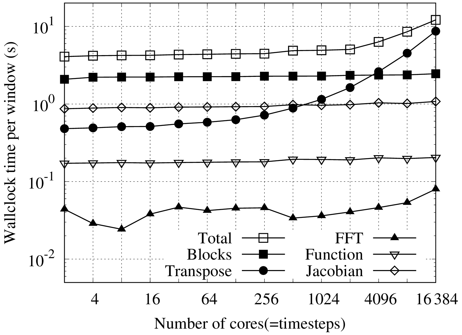
Figure 4 Weak scaling in time profile of the linear scalar advection equation test case with N_x=128², σ=0.8, $\mathit{\alpha }={\mathrm{10}}^{-\mathrm{4}}$, and varying window length N_t. Measured wall-clock times per window for each component of the algorithm: total, block solves, space–time transpose, (I)FFTs, all-at-once function evaluation, and all-at-once Jacobian action.

The first example we show is the linear scalar advection equation, the prototypical hyperbolic PDE

$$\begin{array}{}\text{(39)}& {\partial }_{t}q+\mathit{u}\cdot \mathrm{\nabla }q=\mathrm{0},\end{array}$$

where q is the advected quantity and u is the advecting velocity. This very simple equation demonstrates the fundamental wave propagation behaviour of hyperbolic problems and has proved challenging for many parallel-in-time schemes. This equation has a single characteristic wave travelling at speed $\left|\mathit{u}\right|$. We use this case to demonstrate the linear convergence rate Eq. (14) to be independent of N_t. Measured speedups will be shown versus the performance model predictions in Eq. (31) to verify the efficiency of the time-parallelism implementation in asQ. Speedup results will be presented as strong scaling in time, i.e. wall-clock time taken per time step calculated.

Table 1 Iteration counts m_p, contraction rates η, and measured speedup S for the preconditioned Richardson iterations with varying α and window lengths N_t. The expected contraction rate is ${\mathit{\eta }}_{\mathrm{e}}=\mathit{\alpha }/(\mathrm{1}-\mathit{\alpha })$.

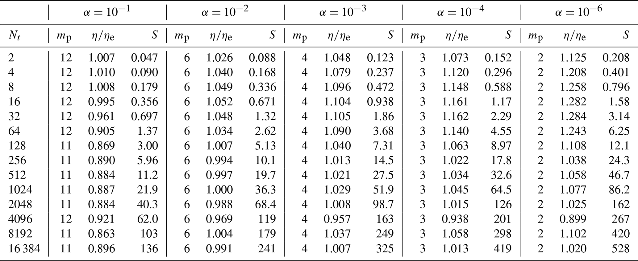
Equation (39) is discretised with a linear discontinuous Galerkin method in space with an upwind flux at the element interfaces and the trapezium rule in time. This discretisation is second order in the L₂ norm in both space and time and is unconditionally stable. The test case is a Gaussian bump advected in a periodic unit square, with a constant velocity u at an angle 30° to the horizontal mesh lines. A quadrilateral mesh with 128² elements is used resulting in ≈ 65 kDoFs per time step, and the Courant number is $\mathit{\sigma }=\left|\mathit{u}\right|\mathrm{\Delta }t/\mathrm{\Delta }x=\mathrm{0.8}$. Using N_T=16384, the window size is increased in powers of 2 from N_t=2 up to $N_t={\mathrm{2}}^{\mathrm{14}}=\mathrm{16}\mathrm{384}$.

The linear system for the block in the serial-in-time method is solved directly using LU factorisation with the MUMPS package (Amestoy et al., 2001, 2019). The factorisation is precalculated and reused across all time steps. The direct solver is also used for the blocks in the circulant preconditioner, meaning that γ=1 in the performance model in Eq. (32). Direct solvers do not scale well at the low DoF count of this case, so for the serial-in-time method we use P_s=1, and in the parallel-in-time method we also use a single core per block, i.e. P_t=N_t instead of P_t=2N_t. This means that the speedup predictions from the performance model must be halved, but it does mean that the parallel results demonstrate only the time parallelism in asQ, independently of Firedrake's existing spatial parallelism.

The all-at-once system is solved to a tolerance of 10⁻¹¹ using preconditioned Richardson iterations. The number of Richardson iterations per window m_p and the measured convergence rates are shown in Table 1 for varying α from 10⁻¹ to 10⁻⁶. The convergence rate for all cases is very close to the $\mathit{\alpha }/(\mathrm{1}-\mathit{\alpha })$ rate predicted by Eq. (14) and varies very little with N_t. For larger α the convergence rate is slightly lower than the theoretical prediction, while for very small α the convergence rate is slightly higher than the theoretical prediction, likely as a result of the increased roundoff error of the diagonalisation. Note that because the Richardson iteration requires one additional preconditioner application to calculate the initial preconditioned residual, the speedup prediction in Eq. (31) is $N_t/\left(\mathrm{2}(m_{\mathrm{p}}+\mathrm{1})\right)$ assuming T_c≪T_b.

The measured wall-clock times per time step $T_{\mathrm{p}}/N_t$ for each value of α are shown in Fig. 3 compared to the serial-in-time method T_s. The corresponding speedups are shown in Table 1. For smaller N_t the available parallelism is not enough to outweigh the overhead of the parallel method, with the crossover to speedup occurring at N_t≈64 for $\mathit{\alpha }={\mathrm{10}}^{-\mathrm{1}}$ down to N_t≈16 for $\mathit{\alpha }={\mathrm{10}}^{-\mathrm{6}}$. The scaling in time is almost perfect from N_t=2 to N_t=1024, achieving 45 %–55 % of the ideal speedup S in Eq. (31) across this range compared to the measured T_s. For larger window sizes the speedup increases further, but the scaling deteriorates, with maximum speedups at N_t=16 384 of 129 with $\mathit{\alpha }={\mathrm{10}}^{-\mathrm{1}}$ up to 517 with $\mathit{\alpha }={\mathrm{10}}^{-\mathrm{6}}$. As α decreases, the speedup increases almost exactly proportionally to the reduction in the iteration count. These speedup results are very competitive with previous state-of-the-art results for the constant coefficient scalar advection equation: 10–15 using ParaDiag with a collocation method (Čaklović et al., 2023) and up to 18 using MGRIT with optimised coarse-grid operators (De Sterck et al., 2021). De Sterck et al. (2023a, b) achieved speedups of up to 12 on variable coefficient advection using MGRIT with modified semi-Lagrangian coarse operators. Although the variable coefficient case follows very naturally for the semi-Lagrangian method, for ParaDiag this case is more difficult because it requires a constant coefficient state in the circulant preconditioner. In this article, problems with variable coefficients are demonstrated using the nonlinear examples below; variable coefficient linear equations are left for later work.

The ideal lower bound on the runtime $T_{\mathrm{s}}/S$ from Eq. (31) using the measured T_s is shown in Fig. 3 for $\mathit{\alpha }={\mathrm{10}}^{-\mathrm{6}}$, labelled $T_{\mathrm{s}}/S\left({\mathit{\alpha }}^{-\mathrm{6}}\right)$. The measured speedup closely follows the prediction until the very longest window lengths. To explore this scaling behaviour, the time taken by the most expensive sections of the computation are shown in Fig. 4. Only the profile for $\mathit{\alpha }={\mathrm{10}}^{-\mathrm{4}}$ is shown as this is the recommended value from Gander and Wu (2019), and the profiles for the other values of α are almost identical. For clarity, the timings are shown per window solve instead of per time step, i.e. multiplied by N_t compared to the times in Fig. 3. With perfect parallel scaling, each window solve would take a constant wall-clock time independent of N_t. Shown are the total time per window solve and the time taken for the block solves, the space–time transpose, the (I)FFTs, evaluation of the all-at-once function Eq. (18), and the action of the all-at-once Jacobian Eq. (21).

We first inspect the operations outside of the preconditioner. The Jacobian action and the function evaluation have the same execution pattern: a one-sided point-to-point communication round to update the time halos, followed by embarrassingly parallel-in-time computation of the result. The Jacobian action takes a longer time, but both scale very well with N_t due to the majority of the time being spent on parallel computation and the communication complexity being independent of N_t.

Next we inspect the operations in the preconditioner. The first point to notice is that, just as for the function and Jacobian action evaluations, the time spent in the block solves in Step 2 scales almost perfectly across the entire range of N_t, as expected due to this step being embarrassingly parallel in time. There is a very slight increase for the highest N_t due to a minor increase in the fill-in of the LU factorisation, but this effect is negligible.

The (I)FFTs are a minimal part of the profile, taking approximately 1 % of the total solution time for all window sizes. The time taken actually decreases as N_t increases up to N_t=512. Each core calculates $N_x/N_t$ transforms of length N_t. The total work required from each core is 𝒪(N_xlogN_t), but it seems that the implementation used (scipy.fft) is more efficient for fewer longer transforms, leading to the initial decrease with N_t, before the gradual increase after that.

Looking at the final component of the preconditioner, it is clear that the space–time transposes are the main culprit for the loss of scaling for large N_t. For N_t≤32 the entire problem fits on a single node, and the communication time is almost constant. For N_t≥64 internode communication is required, and the communication time increases steadily as expected for an Alltoall communication. At N_t=8192 the transpose communications require more time than any other part of the computation, and at N_t=16 384 they take almost 60 % of the total solution time. From Fig. 3 we can see that the scaling behaviour is almost identical for all values of α, which supports the assertion in Sect. 2.3 that $T_{\mathrm{c}}/T_{\mathrm{b}}$ in the performance model depends on N_t but not on the effectiveness of the circulant preconditioner.

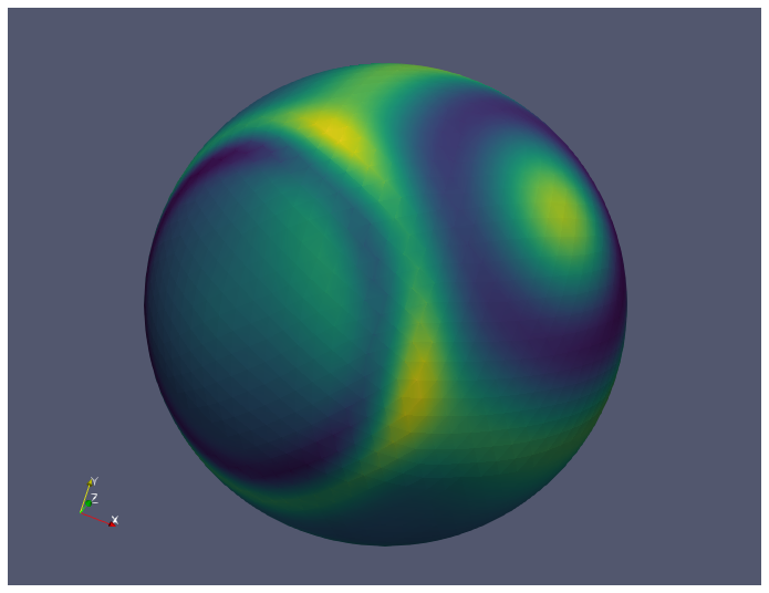
Figure 5 Colour plot of the free surface elevation h in the linear-rotating shallow water equation test case.

4.2 Linear shallow water equations

The next example is the linearised shallow water equations on the rotating sphere. The shallow water equations are obtained by assuming that the vertical (normal to the sphere) length scales of the flow are orders of magnitude smaller than the horizontal (tangential to the sphere) length scales and taking an average over the depth of the fluid. The equations can be further simplified by linearising around a state of rest and a mean depth, which results in the following:

$$\begin{array}{}\text{(40)}& \begin{array}{rl}{\displaystyle }{\partial }_t\mathit{u}+f{\mathit{u}}^{⟂}+g\mathrm{\nabla }h& {\displaystyle }=\mathrm{0},\\ {\displaystyle }{\partial }_{t}h+H\mathrm{\nabla }\cdot \mathit{u}& {\displaystyle }=\mathrm{0},\end{array}\end{array}$$

where u is the velocity perturbation tangent to the sphere around the state of rest, f is the Coriolis parameter due to the rotating reference frame, and ${\mathit{u}}^{⟂}=\mathit{u}\times \widehat{k}$ where $\widehat{k}$ is the unit normal vector to the sphere, g is gravity, and h is the perturbation around the mean depth H. This is an oscillatory PDE system with a hyperbolic part resembling a wave equation, plus the Coriolis term.

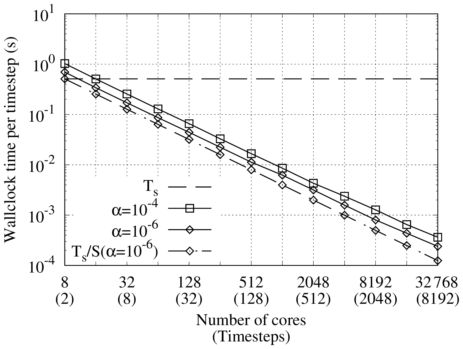
Figure 6 Strong scaling in time of the linear shallow water equations on the rotating sphere with 20 000 elements, dt=900 s, and varying window length N_t for $\mathit{\alpha }={\mathrm{10}}^{-\mathrm{4}}$ and $\mathit{\alpha }={\mathrm{10}}^{-\mathrm{6}}$. P_s=2 for the serial-in-time method and P_p=2N_tP_s for the parallel-in-time method. Measured wall-clock times per time step T_p, as well as the predictions of the performance model $T_{\mathrm{s}}/S$ in Eq. (31) for $\mathit{\alpha }={\mathrm{10}}^{-\mathrm{6}}$ using the measured T_s (assuming T_c=0). The wall-clock time for the serial-in-time method is plotted as the horizontal line. Maximum speedups of 1402 and 2126 with $\mathit{\alpha }={\mathrm{10}}^{-\mathrm{4}}$ and $\mathit{\alpha }={\mathrm{10}}^{-\mathrm{6}}$ respectively, both at P_p=32 768 and N_t=8192.

We use the test case of Schreiber and Loft (2019), which simulates propagation of gravity waves around the Earth's surface and was used to test REXI parallel-in-time algorithms. The initial conditions are zero velocity and three Gaussian perturbations to the depth. As time advances, each Gaussian relaxes into a wave travelling around the globe in all directions, shown in Fig. 5.

Schreiber and Loft (2019) show that the dispersion error of the trapezium rule integration method can lead to higher errors than the REXI schemes. However, here we are primarily concerned with ParaDiag's ability to speed up the calculation of the base integrator, rather than with the ultimate accuracy of the base integrator.

An icosahedral sphere mesh with five refinement levels is used, resulting in ≈20 000 simplex elements. The equations in Eq. (40) are discretised using a compatible finite element method (Cotter, 2023). We choose the quadratic Brezzi–Douglas–Marini elements V_u=BDM₂ for the discrete velocity space (Brezzi et al., 1985) and the linear discontinuous Lagrange elements V_h=DG₁ for the layer depth space. This results in ≈215 kDoFs for each time step of the serial-in-time method.

The blocks in both the serial-in-time and parallel-in-time methods are solved using hybridisation, which is a technique for exactly reducing the block matrix to a smaller finite-element space supported only on the facets between cells. The smaller system is similar to a pressure Helmholtz equation and is solved using LU decomposition with the (u,h) solution obtained exactly by back-substitution. For more detail on hybridisation and its implementation in Firedrake, see Gibson et al. (2020). Using this technique, the block “iteration” counts are k_s=1 and k_p=1, as in the advection example. Although the blocks considered here are tractable with direct methods, full atmospheric models are not, so hybridisation or similar techniques are often used, and for this reason they are interesting to consider for parallel-in-time applications.

The all-at-once system is solved using flexible GMRES (FGMRES; Saad, 1993) to a relative tolerance of 10⁻¹¹ for two α values $\mathit{\alpha }={\mathrm{10}}^{-\mathrm{4}}$ and $\mathit{\alpha }={\mathrm{10}}^{-\mathrm{6}}$, converging in m_p=3 and m_p=2 iterations respectively independently of N_t.³ We achieved greater speedup for $\mathit{\alpha }={\mathrm{10}}^{-\mathrm{6}}$ in the previous example, but we also show $\mathit{\alpha }={\mathrm{10}}^{-\mathrm{4}}$ here because it is closer both to the recommended values (Gander and Wu, 2019) and to those used for the nonlinear problems we consider next, where the predominant error stems from the reference value $\widehat{u}$ in the preconditioner, so decreasing α further does not lead to greater speedup. The serial-in-time problem is parallelised in space with P_s=2 cores, resulting in ≈108 kDoFs per core. In the parallel-in-time method, P_p=2P_sN_t cores are used to maintain the same number of floating points per core for the complex-valued block solves.

The strong scaling of wall-clock time taken per time step is shown in Fig. 6, using N_T=8192 and again increasing N_t in powers of 2, up to N_t=N_T with P_p=32 768. The performance model prediction for $\mathit{\alpha }={\mathrm{10}}^{-\mathrm{6}}$ is also shown. The crossover to the parallel method being faster occurs at N_t=4 for both cases, earlier than for the scalar advection example due to using 2P_s cores for each block solve. Again we see excellent scaling for both cases, achieving 63 %–74 % of the ideal speedup from N_t=2 to N_t=1024, where the actual speedups are 214 and 323 using 4096 cores. For N_t>1024 the scaling deteriorates slightly but still reaches maximum speedups over the serial-in-time method of 1402 and 2126 with N_t=8192 for a total of ≈1.75 billion DoFs using 32 768 cores (512 nodes), or 51 % of the ideal speedup for each value of α. This speedup is very competitive with previous results in the literature for time-parallel speedup of the linear shallow water equations (Schreiber et al., 2018).

ParaDiag can clearly scale excellently and achieve very competitive speedups for linear equations, even hyperbolic ones that have previously proved challenging for parallel-in-time methods. With reference to the performance model in Eq. (31), this scaling relies on three factors. Firstly, the number of all-at-once iterations m_p is fixed independently of N_t. This holds for constant coefficient equations such as we have considered so far because no averaging is necessary in the preconditioner, so the $\mathit{\alpha }/(\mathrm{1}-\mathit{\alpha })$ convergence rate in Eq. (14) is achieved independently of N_t. Secondly, the number of iterations for the complex-valued block solves k_p is fixed independently of N_t. So far we have achieved this either by directly solving the blocks or using hybridisation to reduce the block system down to a size where a direct solver can be applied. Lastly, the collective communications required for the space–time transpose must scale well. In the examples so far this has been the limiting factor on the scaling, although only once N_t is 𝒪(10⁴).

4.3 Nonlinear shallow water equations

The nonlinear shallow water equations on the rotating sphere retain the nonlinear advection terms, which are removed in the linear shallow water equations. Writing the velocity advection in vector invariant form, the nonlinear equations are

$$\begin{array}{}\text{(41)}& \begin{array}{rl}{\displaystyle }{\partial }_t\mathit{u}+(\mathrm{\nabla }\times \mathit{u}+f){\mathit{u}}^{⟂}+{\displaystyle \frac{\mathrm{1}}{\mathrm{2}}}\mathrm{\nabla }|\mathit{u}{|}^{\mathrm{2}}+g\mathrm{\nabla }h& {\displaystyle }=\mathrm{0},\\ {\displaystyle }{\partial }_{t}h+\mathrm{\nabla }\cdot \left(\mathit{u}h\right)& {\displaystyle }=\mathrm{0}.\end{array}\end{array}$$

The same compatible finite element spaces are used as for the linear shallow water equations, using the discretisation presented in Gibson et al. (2019).

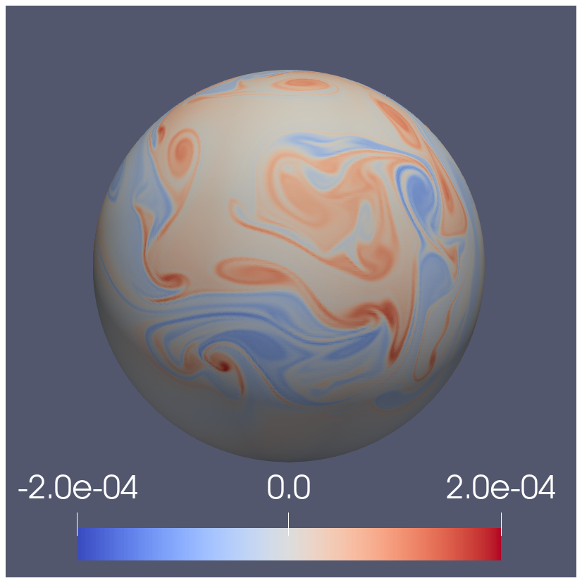
Figure 7 Colour plot of the potential vorticity in the rotating shallow water equation test case.

Table 2 Details on the four refinement levels of the icosahedral sphere mesh used for the unstable jet test case. DoFs include both the velocity and depth DoFs. Δx is the element edge length, and Δt is chosen for an advective Courant number of approximately σ≈0.4. P_s is the number of cores used in the serial-in-time method.

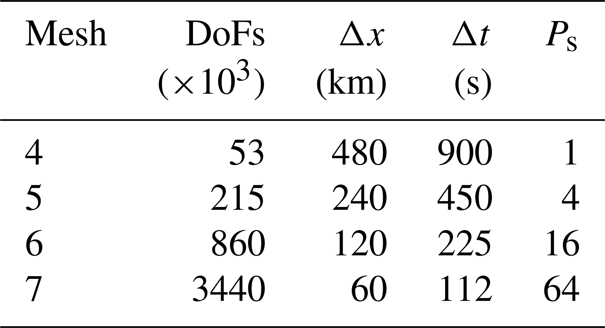
We use the classic test case from Galewsky et al. (2004) of an unstable jet in the Earth's Northern Hemisphere, which breaks down into a highly nonlinear vortical flow over a period of several days. The strong nonlinearities provide a test of the error introduced by the averaging procedure in the circulant preconditioner. The flow is evolved from the initial conditions to a final time of 10 d at a range of resolutions and window lengths N_t. The potential vorticity field at 10 d is shown in Fig. 7. All window lengths tested were much smaller than the total number of time steps required, so multiple windows are solved sequentially until the final time is reached, using the last time step of one window as the initial condition for the next window.

The trapezium rule is used in time, and the time step is scaled with the mesh resolution to keep the advective Courant number close to constant around σ≈0.4 across all tests. The blocks in both the serial-in-time and parallel-in-time methods are solved using the FGMRES Krylov method preconditioned with a geometric multigrid. The relaxation on each grid level is four GMRES iterations preconditioned with a vertex Vanka patch smoother. This is an additive Schwarz method where each subdomain is associated with a mesh vertex and contains all DoFs in the closure of the star of the vertex. The coarsest level is solved directly using MUMPS. For the serial-in-time case this method gives resolution-independent convergence rates for fixed Courant number. The patch smoothers are implemented in PETSc with PCPATCH and exposed in Firedrake through the firedrake.PatchPC interface (Farrell et al., 2021b).

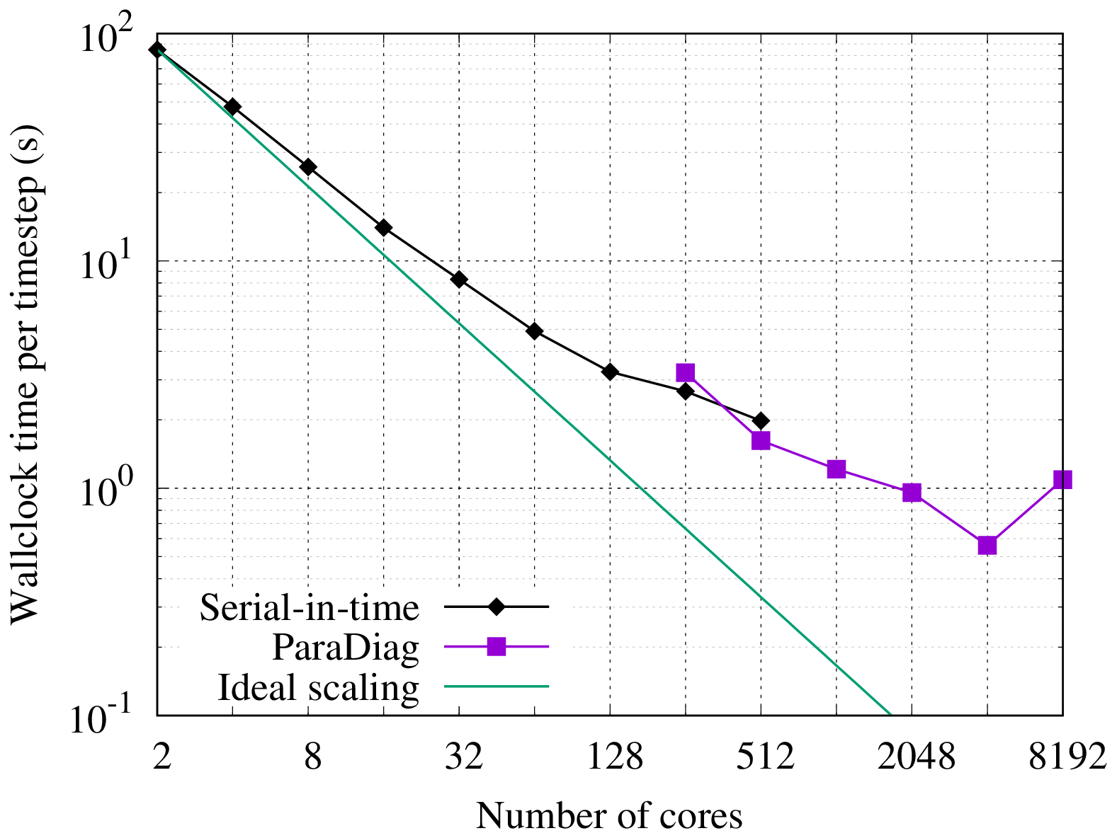
Figure 8 Strong scaling in space or time for the unstable jet shallow water case for the highest resolution, mesh 7 with 3.4 MDoFs per time step. Serial-in-time results show strong scaling in space from P_s=2 to P_s=512. ParaDiag results show strong scaling in time from N_t=2 to N_t=64 with P_p=2N_tP_s and P_s=64. The ideal scaling shows perfect parallel scaling from the serial-in-time result with P_s=2.

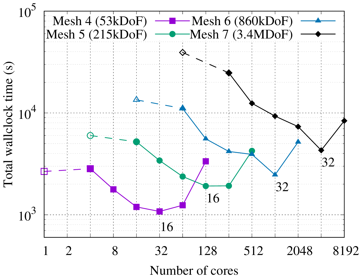
Figure 9 Strong scaling in time for the unstable jet shallow water test case at varying mesh resolutions. Measured wall-clock time to simulate 10 d. On each curve, the leftmost data point with an open symbol shows the serial-in-time (but possibly parallel-in-space) result, and the second data point onwards shows parallel-in-time results at increasing window lengths N_t from 2–64. The number of cores for the parallel-in-time results is P_p=2N_tP_s. Maximum speedups are 2.47, 3.14, 5.45, and 9.12 at refinement levels 4, 5, 6, and 7 respectively. Labels indicate N_t at the maximum speedup on each mesh.

Each time step in the serial-in-time method and each window in the parallel-in-time method is solved using an inexact Newton method with the tolerance for the linear solves at each Newton step determined using the first Eisenstat–Walker method (Eisenstat and Walker, 1996). In the serial-in-time method the convergence criterion is a nonlinear residual below an absolute tolerance of 10⁴, equivalent to around a 10⁻⁶ relative reduction in the residual.⁴ In the parallel-in-time method, a nonlinear residual below $\sqrt{N_t}{\mathrm{10}}^{\mathrm{4}}$ is required, i.e. an average residual of 10⁴ at each time step. In the linear examples we converged to very tight tolerances, which are useful to confirm the convergence of the method but are impractical because, in reality, discretisation errors will be orders of magnitude larger. In practice, the convergence tolerance need only be tight enough for the method to be stable and to reach the expected spatial and temporal convergence rates. The linear solve at each Newton step of the parallel-in-time method is solved using FGMRES using the circulant preconditioner and a value of $\mathit{\alpha }={\mathrm{10}}^{-\mathrm{4}}$, and the complex-valued blocks are solved to a relative tolerance of $\mathit{\tau }={\mathrm{10}}^{-\mathrm{3}}$. The circulant preconditioner will not achieve the expected convergence unless the complex-valued blocks are solved to a relative tolerance τ of at least as small as $\mathit{\alpha }/N_t$ (and often smaller) (Čaklović et al., 2023). For the linear examples we used a direct solver on the blocks, equivalent to a relative tolerance close to machine precision. For operational models direct solvers are unfeasible, both because of the large size of the system and because, for nonlinear systems, a refactorisation would be necessary at each Newton iteration. Here, we use an iterative solver for the blocks, so reducing α requires more expensive block solves. Empirically we have found that setting α and τ in the range 10⁻⁵–10⁻³ gives a good balance between inner/outer Krylov iterations, but exploring and analysing this choice further is left for later work.

Four different refinement levels of the icosahedral sphere mesh are used ranging from 50–3440 kDoFs. See Table 2 for details on each mesh. Before showing parallel-in-time results, we first present a spatial strong scaling study at the largest mesh resolution to quantify how close to saturation the spatial parallelism is. The wall-clock time taken to calculate each time step by the serial-in-time method with varying P_s is shown in Fig. 8, from P_s=2 using a single L3 cache with 1.72×10⁶ DoFs/core to P_s=512 using 8 nodes with 6.7×10³ DoFs/core. At P_s=512 the speedup over P_s=2 is 47.8, giving a parallel efficiency of 19 %, which is almost certainly below the acceptable level for the vast majority of applications. The highest core count that fits on one node is P_s=64 with 53×10³ DoFs/core, giving a speedup over P_s=2 of 17.3 with parallel efficiency of 54 %. At larger P_s the efficiency drops below 50 %. A parallel efficiency of 54 % is approaching saturation in space, without being unreasonably wasteful of resources. In the rest of this section a constant DoFs/core of 53×10³ is used. The corresponding P_s for each mesh is shown in Table 2, and in all parallel-in-time cases we use P_p=2N_tP_s.

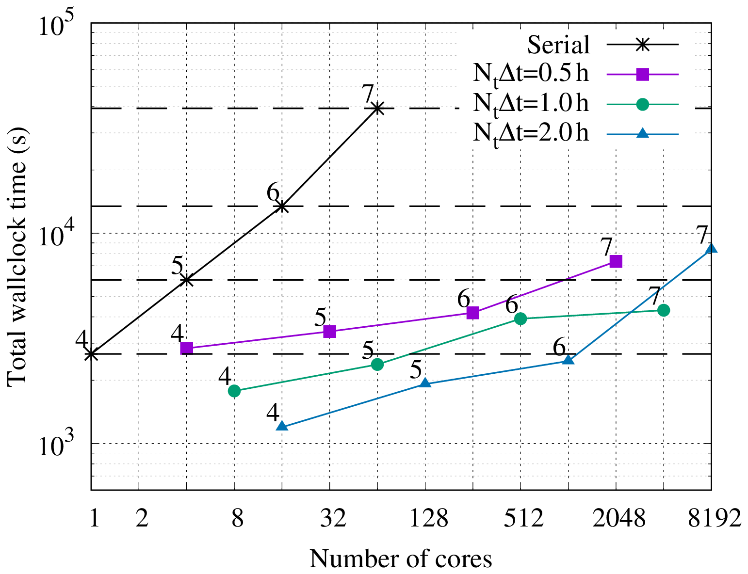
Figure 10 Weak scaling in time and space for the unstable jet shallow water test case. Measured wall-clock time to simulate 10 d at various resolutions. Lines are plotted for increasing resolutions at constant window length T=N_tΔt: for each mesh refinement Δt and Δx are halved and N_t doubled. Data points are labelled with the mesh resolution. $N_t=\mathrm{2},\mathrm{4},\mathrm{8}$ for $T=\mathrm{0.5},\mathrm{1},\mathrm{2}$ respectively on mesh 4. The number of cores for the parallel-in-time results is P_p=2N_tP_s.

For the parallel-in-time results we first show strong scaling of the wall-clock time for 10 simulation days at each mesh resolution for increasing window sizes in Fig. 9. As for the linear problems there is little or no speedup for very small N_t, followed by a close to linear increase in the speedup as N_t grows. However, around N_t=16–32 the speedup reaches maximums of between 2.47 and 9.12 for the lowest and highest resolution respectively over the equivalent serial-in-time method. Although these speedups are significantly less than those achieved for linear problems, they are competitive with current state of the art parallel-in-time methods for the shallow water equations, without any modification to the basic ParaDiag algorithm.

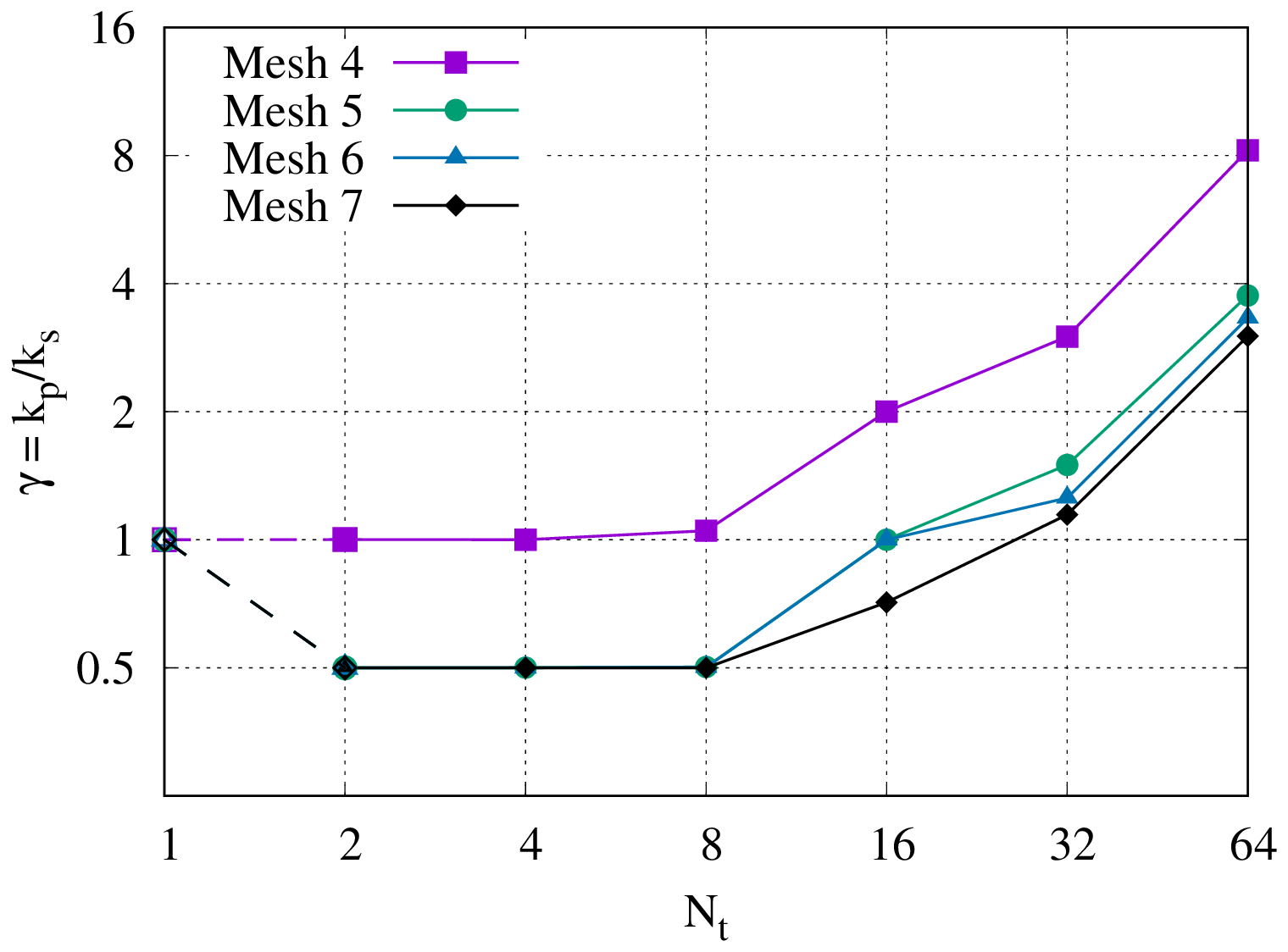
Figure 11 Scaling of the block iteration counts for the nonlinear shallow water equations $\mathit{\gamma }=k_{\mathrm{p}}/k_{\mathrm{s}}$, with maximum iteration counts for the complex-valued blocks in the circulant preconditioner k_p and block iteration counts for the real-valued blocks in the serial-in-time method k_s. The ratio γ is plotted versus the window length N_t for each mesh resolution. The data point at N_t=1 is ${\mathit{\gamma }}_{\mathrm{s}}=k_{\mathrm{s}}/k_{\mathrm{s}}=\mathrm{1}$.

In Fig. 8 we can compare the performance of continuing to strong scale in space past P_s=64 vs. switching to strong scaling in time. Although at N_t=2 with P_p=256 the parallel-in-time speedup is immediately higher than the serial-in-time method with P_s=64, the serial-in-time method with the same number of cores is still slightly faster. However, at N_t=4 with P_p=512, the parallel-in-time method just overtakes the serial-in-time method with the same number of cores, with both methods reaching speedups over P_s=2 of around ≈50. The fastest case, with N_t=32 and P_p=8192, reaches speedups of 9.12 over the serial-in-time method with P_s=64 and 152 over P_s=2. Although the crossover to time parallelism giving greater scaling than spatial parallelism here is fairly low at N_t=4, this may vary slightly depending on which P_s is used as the reference point to calculate P_p=2N_tP_s. Using a larger P_s would increase the overall speedup of the parallel-in-time method but of course with worse parallel efficiency.

For all mesh resolutions there is a sudden and drastic reduction in the parallel-in-time speedup in Fig. 9 at N_t=64. To understand this behaviour we return to the performance model in Sect. 2.3. For all four mesh resolutions, the serial-in-time method required two Newton steps (m_s=2), with one multigrid cycle per step for resolution 4 and two cycles per step for all other resolutions (i.e. k_s=1 or 2). The block iteration parameter $\mathit{\gamma }=k_{\mathrm{p}}/k_{\mathrm{s}}$ is shown in Fig. 11, and the number of linear all-at-once iterations required per window m_p is shown in Fig. 12. Both iteration counts increase with N_t, eventually resulting in the performance degradation seen in Fig. 9. We now examine each parameter in more detail.

In Fig. 11, the increase in the iterations is due to the clustering of the circulant eigenvalues close to the imaginary axis shown in Fig. 1. For small window lengths the blocks for meshes 5, 6, and 7 only require a single iteration to reach the required tolerance versus two for the serial-in-time block, which contributes significantly to the improved speedups for higher resolutions. This lower iteration count is achieved because, although the block coefficients are less favourable in the complex-valued case, we do not require a very tight tolerance. The major error in the preconditioner is the averaging error, discussed below, which means that as long as the error from the inexact block solves is below the averaging error, there is no further gain in the convergence of the all-at-once system from solving the blocks to a tighter tolerance.

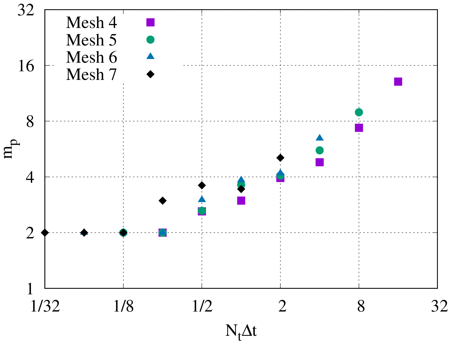
Figure 12 Scaling of the all-at-once iteration counts for the nonlinear shallow water equations. We show iteration counts m_p for all mesh resolutions and window sizes versus the window duration N_tΔt in hours, where Δt depends on the mesh resolution due to the constant Courant number.

In Fig. 12 the number of linear all-at-once iterations across all Newton steps per window m_p is plotted against the total window duration T=N_tΔt. We see that the data for the different resolutions collapse onto each other, and, after an initial plateau at m_p=2, the number of all-at-once iterations scales close to linearly with T. This is consistent with a convergence rate scaling of κN_tΔt for the averaged preconditioner (Čaklović, 2023), assuming that the Lipschitz constant κ is a function of the underlying continuous problem and so is essentially constant with resolution. This scaling is the primary reason why the maximum speedup increases with mesh resolution in Fig. 9: in order to balance spatial and temporal errors, Δt is decreased proportionally to Δx to maintain a constant Courant number, so for the same N_t the higher-resolution meshes have better convergence rates of the all-at-once system.⁵

Next we investigate the effectiveness of weak scaling in both time and space. Previously we were interested in decreasing the wall-clock time at a particular resolution. Now we are interested in solving to a fixed final time and increasing the spatial and temporal resolution simultaneously without increasing the wall-clock time. This represents the situation where we would like to provide a more accurate forecast of a particular length at a particular delivery frequency.

We investigate the weak scaling for the unstable jet case by reinterpreting the data in Fig. 9, selecting a particular window duration T=N_tΔt and keeping this fixed as the resolution is increased: each time the mesh is refined, Δx and Δt are halved and N_t is doubled. The results for window durations of 0.5, 1, and 2 h are shown in Fig. 10, alongside the wall-clock times for the serial-in-time method weak scaled only in space. As expected from the performance model in Eq. (27), the wall-clock time for the serial-in-time method increases linearly with resolution despite almost perfect weak scaling in space because the total number of time steps increases. On the other hand, the parallel-in-time method scales much more favourably, with the exception of the highest resolution (mesh 7) data point on the longest time window $T=N_t\mathrm{\Delta }t=\mathrm{2}$ h, which corresponds to the N_t=64, P_p=8192, and data point on the mesh 7 line in Fig. 9. Figure 10 shows that by exploiting time parallelism the resolution can be increased fourfold in both time and space without increasing the total time to solution. This can be seen from the mesh 6 solution with T=2 h requiring the same wall-clock time as the serial-in-time mesh 4 solution or the mesh 7 solution with T=1 h (and almost with T=0.5 h) requiring less wall-clock time than the serial-in-time mesh 5 solution. The all-at-once iteration scaling in Fig. 12 is a key component in achieving this weak scaling behaviour because it shows that the convergence of the all-at-once system with the time-averaged preconditioner is independent of both spatial and temporal resolution for fixed T.

4.4 Compressible Euler equations

The final example we present is the compressible Euler equations restricted to a 2D vertical slice of the atmosphere. This model is an important step in the hierarchy of atmospheric models because, unlike the shallow water equations which only support surface gravity waves, the vertical slice model supports internal gravity waves and acoustic waves (Melvin et al., 2010). The compressible Euler equations with prognostic variables of velocity u, density ρ, and potential temperature θ, with the equation of state for the Exner pressure Π are

$$\begin{array}{}\text{(42)}& \begin{array}{rl}{\displaystyle }{\partial }_t\mathit{u}+\mathit{u}\cdot \mathrm{\nabla }\mathit{u}+f{\mathit{u}}^{⟂}+c_{\mathrm{p}}\mathit{\theta }\mathrm{\nabla }\mathrm{\Pi }+g\widehat{k}& {\displaystyle }=\mathrm{0}\\ {\displaystyle }{\partial }_t\mathit{\theta }+\mathit{u}\cdot \mathrm{\nabla }\mathit{\theta }& {\displaystyle }=\mathrm{0}\\ {\displaystyle }{\partial }_t\mathit{\rho }+\mathrm{\nabla }\cdot \left(\mathit{u}\mathit{\rho }\right)& {\displaystyle }=\mathrm{0}\\ {\displaystyle }{\mathrm{\Pi }}^{(\mathrm{1}-\mathit{\kappa })/\mathit{\kappa }}& {\displaystyle }=R\mathit{\rho }\mathit{\theta }/p_{\mathrm{0}},\end{array}\end{array}$$

where c_p is the specific heat at constant pressure, R is the gas constant, $\mathit{\kappa }=R/c_{\mathrm{p}}$, p₀ is the reference temperature, and f and $\widehat{k}$ are again the Coriolis parameter and unit vector in the vertical direction respectively. We use the compatible finite element formulation proposed in Cotter and Shipton (2023) on a Cartesian mesh, where the finite element spaces are defined as tensor products of 1D elements in the horizontal (x) (x) and vertical (z) directions. This tensor product structure is enabled by Firedrake's ExtrudedMesh functionality, where a 1D horizontal base mesh along the ground is first defined and then extruded in the vertical direction (McRae et al., 2016; Bercea et al., 2016). More details on the properties of this discretisation can be found in Cotter and Shipton (2023). Results will be shown for a classic test case from Skamarock and Klemp (1994) of a gravity wave propagating through a uniform background velocity in a nonhydrostatic regime with f=0 and the flow restricted to in-plane motion only. This test case has been previously used to test the vertical slice discretisations in Cotter and Shipton (2023) and Melvin et al. (2010). The domain has a width and height of 300 km × 10 km and periodic boundary conditions in the horizontal direction. The flow is initialised with background temperature and density profiles ρ_ref and θ_ref in hydrostatic balance and a uniform horizontal velocity u_ref. In the centre of the domain, a small-amplitude temperature perturbation with a length scale of 5 km is added to the background state, which creates an internal gravity wave that propagates to the right and left. The temperature perturbation around the background state is shown in Fig. 13 after 3000 s.

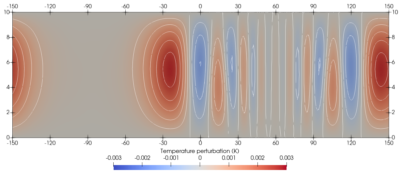
Figure 13 Colour plot of the temperature variation around the back ground state for the compressible Euler internal gravity wave example after 3000 s. Contours are drawn every $\mathrm{5}\times {\mathrm{10}}^{-\mathrm{4}}$ K, and axes labels are in kilometres. Vertical axis is scaled by ×10 for clarity.

The domain is discretised with a resolution of 1 km in both the vertical and horizontal directions, giving 49.2 kDoFs per time step, and the time step size is Δt=12 s, giving an advective Courant number of σ_u≈0.24. Both the serial-in-time and parallel-in-time methods are run for 1024 time steps, with window sizes of N_t=2–128 with the parallel-in-time method (this gives a simulation time longer than the standard end time of 3000 s but results in a minimum of eight windows with the parallel-in-time method). For the serial-in-time method, P_s=2, and for the parallel-in-time method P_p=2N_tP_s.

Cotter and Shipton (2023) used the trapezium rule for serial-in-time integration, with the real-valued block solved using an additive Schwarz method with columnar patches. The patches are constructed as the vertical extrusion of a star patch at each vertex of the base mesh, i.e. collecting all DoFs associated with a vertical column of facets and the interior DoFs of the neighbouring elements and solved using a direct solver. Cotter and Shipton (2023) found that this method has iteration counts that are independent of resolution for fixed Courant number but grow linearly with the Courant number at fixed resolution. When increasing resolution in practice, space and time would usually be refined simultaneously, so constant iteration counts for fixed Courant number is a favourable result. This preconditioner is implemented using Firedrake's ASMStarPC class, which in turns wraps PETSc's PCASM preconditioner and makes use of the fact that ExtrudedMesh retains the topological information of the base mesh to identify the columns.

The first set of results for this example uses the star patch preconditioner for both the real- and complex-valued blocks. The patch preconditioner is constructed from the constant-in-time reference state with non-zero velocity (${\mathbf{u}}_{\mathrm{ref}},{\mathit{\rho }}_{\mathrm{ref}},{\mathit{\theta }}_{\mathrm{ref}})$, which avoids rebuilding the patches through the simulation. Compared to constructing the patches from the current state at each time step, constructing the patches from this reference state gives almost identical iteration counts because the gravity wave variations around the background state are relatively small. For other vertical slice test cases the patches could be constructed around the current state. In the serial-in-time method each time step is solved using Newton-FGMRES with the first Eisenstat–Walker adaptive convergence criteria to an absolute tolerance of 10⁻⁴, giving a relative residual drop of approximately 10⁻⁶. With the patch preconditioner, each time step converged with an average of 27.5 linear iterations across two quasi-Newton iterations with Δt=12 s. The parallel-in-time method is solved using Newton-FGMRES iterations to an absolute tolerance of $\sqrt{N_t}{\mathrm{10}}^{-\mathrm{4}}$ so that the average residual of each time step matches the serial-in-time method. The circulant preconditioner uses $\mathit{\alpha }={\mathrm{10}}^{-\mathrm{5}}$, and each block in Step 2 is solved to a relative tolerance of $\mathit{\tau }={\mathrm{10}}^{-\mathrm{5}}$.

Table 3 Maximum wall-clock speedups achieved by the parallel-in-time method with three different block solution methods (star patch, or the composite preconditioner with either fixed τ or fixed k_p) over the serial-in-time method with two different block solution methods (star patch or the composite preconditioner). The serial-in-time method with the star patch was $\approx \mathrm{1.3}\times$ faster than with the composite preconditioner.

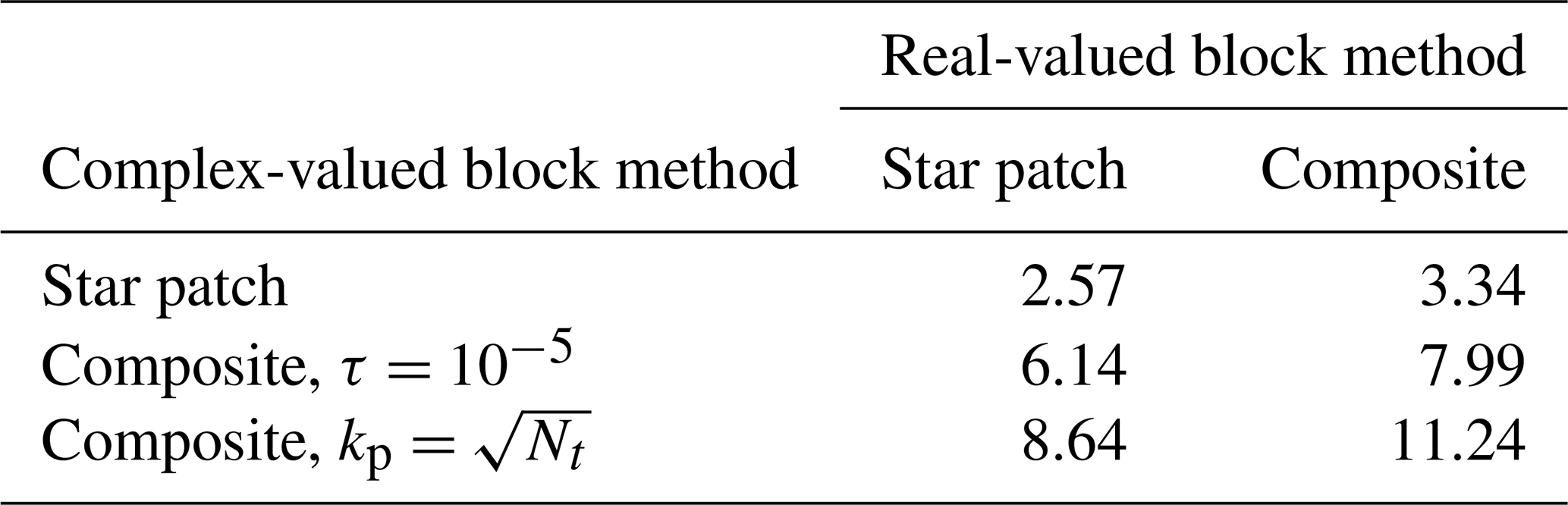
The wall-clock time achieved with this method is shown in Fig. 14 for window lengths N_t=2–32, compared to the serial-in-time method (the “Star” and “Serial (star)” curves respectively). The scaling is underwhelming compared to the previous examples, reaching a maximum speedup of 2.57 at N_t=8 (shown in the top left entry in Table 3). The all-at-once iterations m_p and block iterations k_p are shown in Figs. 16 and 15 respectively. m_p is quite well behaved, remaining at 3 for N_t≤16 before jumping to 6 at N_t=32. We would expect m_p to increase more slowly than the previous example because, although the Euler equations are nonlinear, the gravity wave variations around the background state are relatively small. On the other hand, k_p increases immediately compared to the serial-in-time iteration count k_s and grows quickly with N_t. For this test we had set the maximum number of block iterations to 200 (already an impractically large number). At N_t=32, 18 of the 32 blocks reached the maximum iterations, meaning that the expected tolerance τ was not reached, leading to a deterioration in the effectiveness of the circulant preconditioner and ultimately to the doubling in m_p from N_t=16 to N_t=32. We attribute the growth in k_p to the fact that the coefficients ψ_j in Eq. (16) for some blocks approach the imaginary axis as N_t increases and that the patch method gives iteration counts that grow linearly with the Courant number. Although the patch preconditioner is suitable for the serial-in-time method, clearly a different approach is necessary for an effective ParaDiag method.

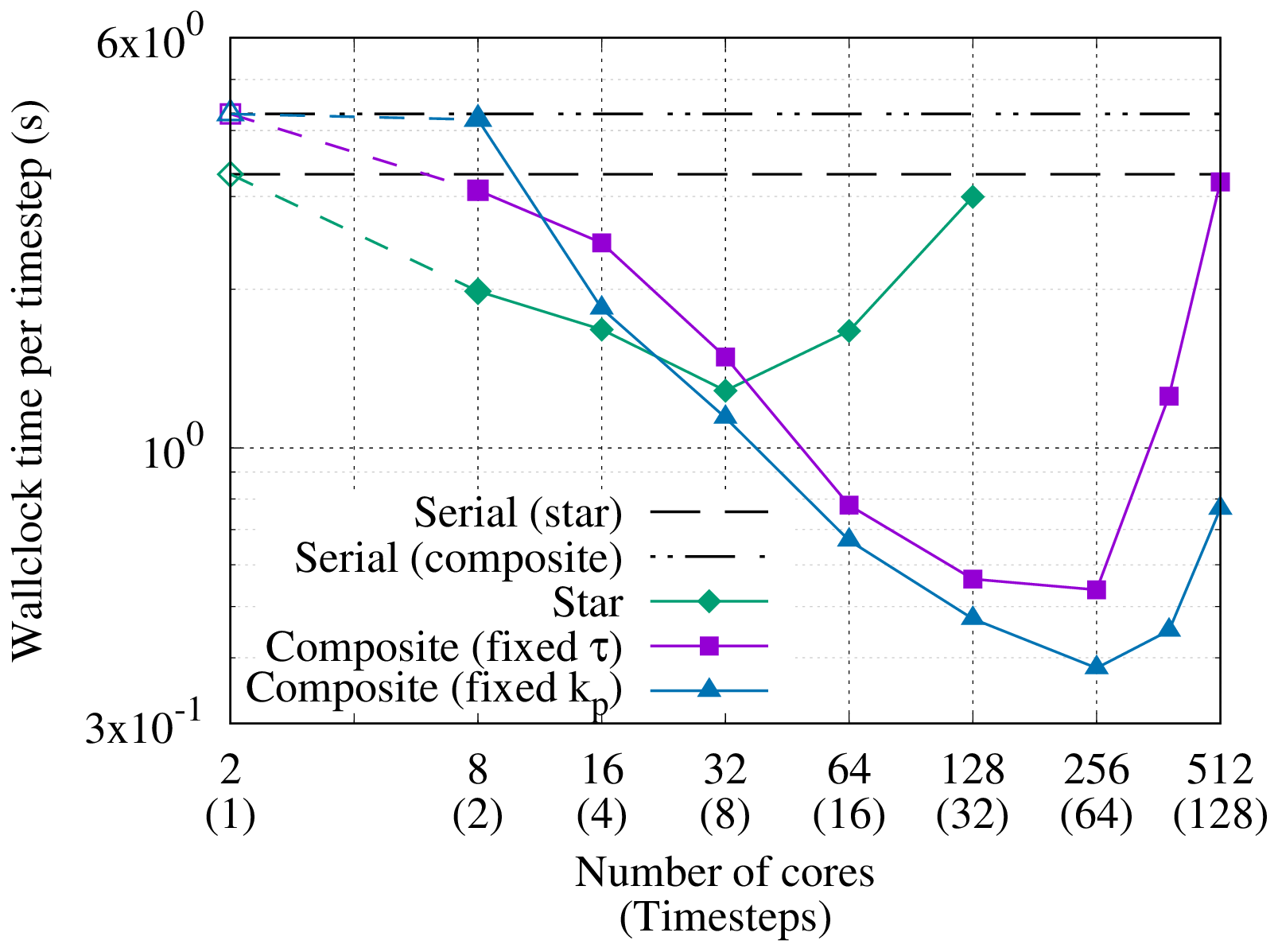
Figure 14 Strong scaling in time of the compressible Euler equations gravity wave test case for varying window length N_t. P_s=2 for the serial-in-time methods, and P_p=2N_tP_s for the parallel-in-time methods. Measured wall-clock times per time step T_p shown for three block solution methods: the star patch, the composite preconditioner with a fixed block tolerance $\mathit{\tau }={\mathrm{10}}^{-\mathrm{5}}$, and the composite preconditioner with a fixed number of block iterations $k_{\mathrm{p}}=\sqrt{N_t}$. The wall-clock times per time step T_s for the serial-in-time methods with the star patch or composite preconditioner are shown at N_t=1 in open symbols and plotted with horizontal lines. Maximum speedups for the parallel-in-time methods over each serial-in-time method are shown in Table 3.

The patch preconditioner iteration counts grow linearly with the Courant number because the domain of dependence of each application of the preconditioner remains constant, while the physical domain of dependence grows linearly with Δt. Therefore, we propose to compose the patch preconditioner multiplicatively with a second preconditioner. This second preconditioner is constructed from Eq. (42) linearised around a reference state at rest $(\mathbf{u},\mathit{\rho },\mathit{\theta })=(\mathbf{0},{\mathit{\rho }}_{\mathrm{ref}},{\mathit{\theta }}_{\mathrm{ref}})$. An LU factorisation of this matrix is calculated at the start of the simulation and reused throughout the time series.⁶ We expect that this composition may improve performance because the two preconditioners are complementary, in the sense that the linearisation around a state of rest targets the wave terms and provides global coupling but lacks the advection terms, whereas the patch smoother handles advection well locally but lacks globalisation. The full block solution strategy is then FGMRES, preconditioned with the composition of the following: two GMRES iterations preconditioned with the linearisation around a reference state at rest, followed by two GMRES iterations preconditioned with the column patch preconditioner (we experimented with combinations of one or two iterations for each inner GMRES method and found (2,2) to have the best performance).

This composition is implemented using PETSc's PCComposite preconditioner. The linearisation around the reference state of rest is implemented by passing the reference state in the appctx Python dictionary to the AuxiliaryRealBlockPC and AuxiliaryComplexBlockPC preconditioners in the serial-in-time and parallel-in-time methods respectively. Implementing this solution strategy required only two small modifications to the code compared to using just the patch smoother. The first was to update the 'circulant_block' PETSc options in the Python dictionary of options to use 'pc_type': 'composite' and to add the sub-options for each of the two preconditioners described above. The second was to create a new Firedrake Function to hold the reference state at rest and pass this into the appctx for the auxiliary preconditioners.

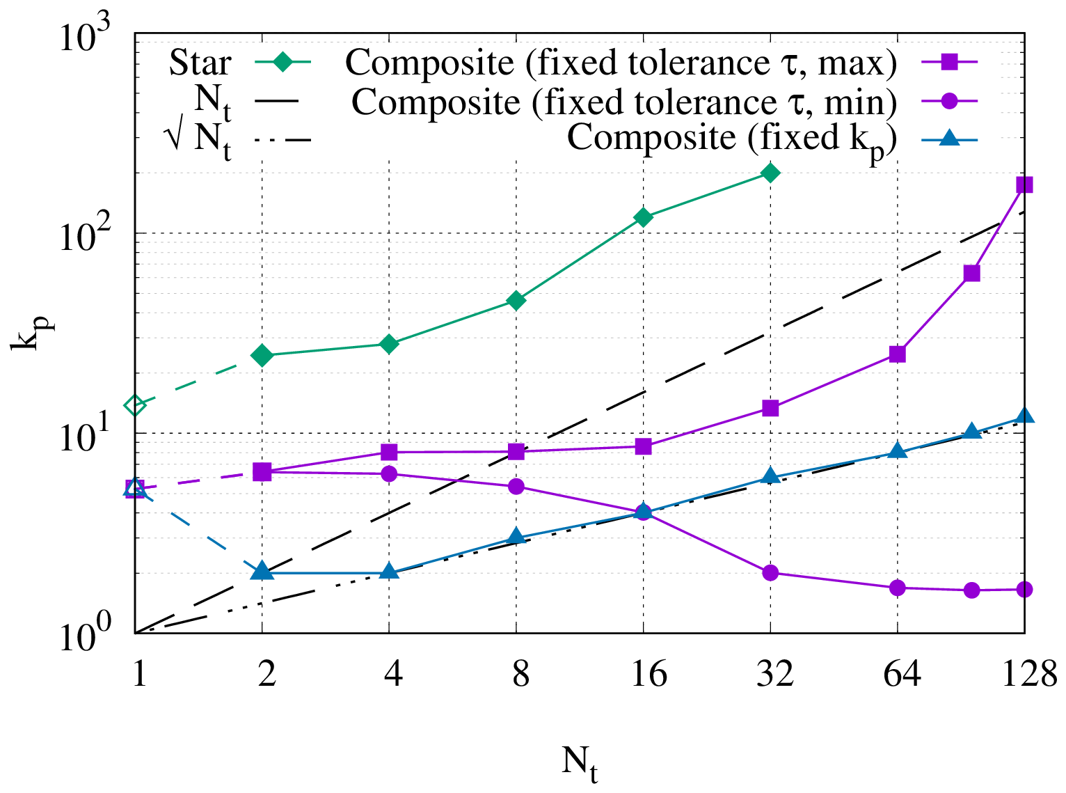
Figure 15 Scaling of the block iteration counts k_p for the compressible Euler equations gravity wave test case at varying window length N_t. Three different preconditioning methods shown: star patch, composite preconditioner with fixed $\mathit{\tau }={\mathrm{10}}^{-\mathrm{5}}$ (for which both maximum and minimum block iteration counts are shown), and composite preconditioner with k_p held fixed at $k_{\mathrm{p}}=\sqrt{N_t}$ (rounded up). The iteration counts for the serial-in-time methods k_s are shown as open symbols at N_t=1 (identical for all composite preconditioner methods).

The wall-clock times required per time step for the serial-in-time method and the parallel-in-time method with increasing window sizes N_t=2–128 using the composite block preconditioner are shown in Fig. 14 (the “Serial (composite)” and “Composite (fixed τ)” curves respectively). The serial-in-time method requires an average of 10.5 block iterations over two Newton iterations per time step, which is actually slightly slower than the patch preconditioner for this Courant number. The parallel-in-time method with the composite preconditioner is also slightly slower than with the patch preconditioner for N_t≤8 but continues to scale at larger window sizes. At N_t=32 the speedup over the serial-in-time method with the composite preconditioner is 7.99, and the speedup over the serial-in-time method with the patch preconditioner is 6.14 (second row of Table 3). The speedup is almost identical at N_t=64, before deteriorating at larger N_t. Nonetheless, this demonstrates that the composite preconditioner gives a more performant method, with a 2.39× improvement on the maximum speedup.

The average number of block inner Krylov iterations for the most difficult block k_p and that of all-at-once outer Krylov iterations m_p, shown in Figs. 15 and 16 respectively for the composite preconditioner (the “composite (fixed tolerance τ, (max))” curves), both increase with N_t but much more gradually than with the patch preconditioner. The block iterations k_p are almost constant until N_t=16 before increasing for larger window lengths. The all-at-once iterations m_p remain almost constant until a longer window length N_t≤64, but a linear increase is seen for N_t>64. This is not due to under-converged blocks in the circulant preconditioner as was the case with the patch preconditioner – no blocks reached 200 iterations – but simply due to the longer window lengths. These combined effects cause the loss of wall-clock scaling around N_t=32 N_t=32, seen in Fig. 14.

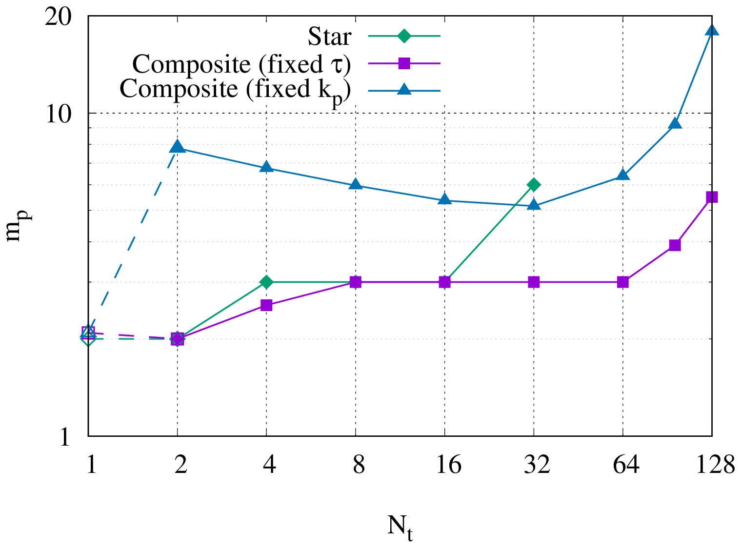
Figure 16 Scaling of the all-at-once outer Krylov iteration counts m_p for the compressible Euler equations gravity wave test case with varying window length N_t. Iteration counts shown when the block convergence tolerance is held fixed at $\mathit{\tau }={\mathrm{10}}^{-\mathrm{5}}$ or when the block iterations are held fixed at $k_{\mathrm{p}}=\sqrt{N_t}$. The iteration count for the serial-in-time method m_s is shown as open symbols at N_t=1.

The number of iterations required for $\mathit{\tau }={\mathrm{10}}^{-\mathrm{5}}$ for the easiest complex-valued block is also shown in Fig. 15 (the “composite (fixed tolerance τ, min)” curve) and actually decreases with N_t. This block always corresponds to the furthest right point of each line in Fig. 1, i.e. the block whose coefficients resemble a very small real-valued time step, which is known to be a favourable condition for iterative solvers. The trends of the maximum and minimum block iterations suggest a further modification to the solution strategy. Instead of fixing the required residual drop for the block solves, we could instead fix the number of iterations k_p to be constant for all blocks, somewhere between the maximum and minimum iterations required for a fixed residual drop. The hope is that “oversolving“ the easiest blocks will mitigate “undersolving” the most difficult blocks enough that the performance of the all-at-once circulant preconditioner does not deteriorate too significantly. As an example, we fix $k_{\mathrm{p}}=\sqrt{N_t}$ (rounding up when $\sqrt{N_t}$ is not an integer). This particular scaling is somewhat arbitrary, but importantly it scales sublinearly with N_t.

The “composite (fixed K_p)” plot in Fig. 16 shows that the number of all-at-once iterations required is increased by this strategy, by a factor of between 1.7–2.1 for N_t=8–64 but rising to a factor of 3.7 at N_t=128. In comparison k_p is reduced by a factor of 3.1 at N_t=64. In Fig. 14 we can see that fixing the block iterations in this way improves the speedup for all window lengths and extends the strong scaling from N_t=32 to N_t=64 compared to fixing the block tolerance. At N_t=64 a speedup of 11.24 over the serial-in-time method with the composite preconditioner is achieved, and a speedup up over the serial-in-time method with the patch preconditioner of 8.64, constituting an improvement of 1.41× over using a fixed block tolerance, and 3.37× greater speedup than the parallel-in-time method with the patch preconditioner (last row in Table 3). If a more sophisticated solver than LU were used for the linearisation around a state of rest (e.g. a Schur complement reduction), we would expect the speedup of the composite method to improve further. We clarify that we are not advocating for fixing k_p specifically to $\sqrt{N_t}$ as a general strategy, rather demonstrating that in some cases it is possible to improve overall performance by “trading” computational work between the inner block iterations and the outer all-at-once iterations. More work is needed in the future to investigate leveraging inexact block solves and differing convergence levels between the blocks to improve performance, guided by the estimates of Čaklović et al. (2023) in their Lemma 3 for the error produced by an inexact application of the circulant preconditioner due to finite machine precision and inexact block solves. They use this error estimate to derive a method for adapting α for fixed τ and discuss the trade-offs between block tolerance and the outer convergence. However, varying α has less impact for nonlinear problems where the dominant error is the time-averaged reference state and would require recalculating any factorisations in the block solution method at every outer Krylov iteration, so specifying τ may be a more effective strategy.

This example shows not only that ParaDiag can produce speedups over serial-in-time methods for the compressible Euler equations, but also that sophisticated solvers can be created and tested using only standard PETSc, Firedrake, and asQ components. As stated in Sect. 3 as part of the aims of asQ, this flexibility is essential for developing ParaDiag into a practical method for use in real applications.

5 Summary and outlook

5.1 Summary

We have introduced a new software library, asQ, for developing the ParaDiag-II family of parallel-in-time methods. ParaDiag-II provides a parallelisable method for solving multiple time steps of classical time steppers, with the implicit θ-method used in asQ. By building on the Firedrake finite element library, Unified Form Language (UFL), and PETSc (the Portable, Extensible Toolkit for Scientific Computation), the design of asQ is intended to improve the productivity of method developers by minimising the effort required to implement a new model or method, thereby maximising the time spent testing said models or methods.

asQ automates the construction of the all-at-once system and the associated Jacobian and preconditioners using Firedrake. Implementing this construction is often a very time-consuming step in the development cycle, which here is achieved solely from a user-provided high-level mathematical description of the finite element model using UFL. While the construction is automated, the user is given full control over the solution of the all-at-once system. This control is predominantly achieved with PETSc options, provided via Python dictionaries or command line arguments. The options interface enables a wide array of solution methods provided by PETSc, Firedrake, and asQ to be selected and switched between with zero, or minimal, changes to the code. asQ also supports the user providing additional states or finite element forms to construct more complex solution methods which cannot be specified solely through the dictionaries of options.

Space–time parallelism is implemented in MPI, and the vast majority of asQ's API is collective over both time and space, with the user only required to specify how many cores to use for parallelism in the time dimension. As such, users need very little expertise with parallel computing to be able to run in parallel and to profile the performance of their methods.

We have used asQ to demonstrate ParaDiag methods on a set of test cases relevant to atmospheric modelling. The demonstrations have shown, firstly, that asQ achieves the expected convergence rates for ParaDiag and that the parallel implementation scales to over 10 000 cores. Secondly, we have shown that ParaDiag is capable of achieving excellent speedup over the equivalent serial-in-time method for linear, constant coefficient equations. For nonlinear problems, some speedup can be achieved but at a much more modest level due to two factors.

1. The constant-in-time reference state approximation in the preconditioner leads to increasing errors as the window duration grows.

2. The complex coefficients of the block linear systems in the preconditioner become less favourable as the number of time steps in the window grows.

The success of ParaDiag methods for nonlinear and nonconstant-coefficient problems will be determined by how effectively these two issues can be overcome.

5.2 Outlook

There are a variety of interesting directions for future research, a few of which we describe here: firstly for further development of the asQ library and secondly for development of ParaDiag methods.

5.2.1 asQ library

Currently, asQ supports only the implicit θ-method time integrator, but implementing other time integrators would be a very useful extension. For example, implicit Runge–Kutta methods have recently been implemented with Firedrake in the Irksome library (Farrell et al., 2021a; Kirby and MacLachlan, 2024). Irksome generates the UFL and preconditioners for the coupled stage system, which could in turn be used to create the Runge–Kutta all-at-once system and corresponding circulant preconditioner in asQ.

Other diagonalisations could also be implemented, such as the direct diagonalisation of ParaDiag-I (Maday and Rønquist, 2008). The roundoff error for direct diagonalisation grows faster with N_t than in the α-circulant approach; however, direct diagonalisation may be more competitive for nonlinear problems where the averaging error currently limits ParaDiag to fairly small N_t.

There are also open questions on ideal implementation strategies. For example, some of the complex-valued blocks in the circulant preconditioner are much easier to solve than others. The parallel efficiency of this step could be improved by load balancing, i.e. solving multiple easier blocks on the same communicator.

5.2.2 ParaDiag methods

Future improvements of ParaDiag, especially for nonlinear problems, must tackle the two issues identified above: preconditioning the complex-valued blocks and overcoming the averaging error for long time windows. We are currently investigating developments in both directions using the nonlinear shallow water equations as a testbed.

Effective preconditioning for the complex-valued blocks will depend on the PDE being solved. For atmospheric models, the blocks include both wave propagation and advection terms. Given the difficulty in solving both high-wavenumber Helmholtz equations and high Courant number advection equations, preconditioners that either tackle both components explicitly or reduce the system to a size tractable by direct methods are likely necessary. This could entail composite preconditioners, similar to that used for the compressible Euler equations above or preconditioners based on Schur complement factorisations.

Diagonalisation in time requires the preconditioner to be a sum of Kronecker products, which in turn requires a constant-in-time spatial Jacobian. As such, overcoming the averaging error will require alternate solution strategies, for example splitting the time series into smaller chunks which can each be preconditioned with a circulant preconditioner, thereby decreasing the averaging error in each chunk. At the linear level, this could resemble a block Jacobi preconditioner for the all-at-once system (see the SliceJacobiPC in Appendix C). At the nonlinear level, one of the simplest options is to parallelise over the quasi-Newton iterations of several all-at-once systems, which is essentially a pipelined nonlinear Gauss–Seidel method, for which we have some promising preliminary results.

ParaDiag methods currently comprise a very active area in the parallel-in-time field, with many possible research directions. The library presented here provides a sandbox for implementing and testing these methods, enabling faster development of new approaches as well as scalable performance demonstrations.

Appendix A: Nomenclature

B1	Time-integrator Toeplitz matrix for M.
B2	Time-integrator Toeplitz matrix for K.
C1	Circulant Toeplitz matrix for M.
C2	Circulant Toeplitz matrix for K.
Dj	Eigenvalue matrix of Cj.
E	Parallel efficiency.
Ix	Identity matrix of size Nx.
K	Stiffness matrix.
M	Mass matrix.
S	Speedup $T_{\mathrm{s}}/T_{\mathrm{p}}$.
T	Final simulation time.
V	Weighted discrete Fourier matrix.
Nx	Number of spatial DoFs.
Nt	Number of time steps.
Ws	Work for the serial-in-time method.
Wp	Work for the parallel-in-time method.
Ts	Time taken for the serial-in-time method.
Tp	Time taken for the parallel-in-time method.
Tb	Time taken per block solve in preconditioner P.
Ps	Processors used for the serial-in-time method.
Pp	Processors used for the parallel-in-time method.
b	PDE forcing term.
$\stackrel{\mathrm{̃}}{b}$	Discretised forcing term.
cj	First column of Cj.
f	Nonlinear function of u.
g	Error function for the Jacobian averaging.
$\widehat{f}$	Reference function for 𝒫.
ks	Number of Krylov iterations per block solve for the serial-in-time method.
kp	Number of Krylov iterations per block solve for the parallel-in-time method.
ms	Number of Newton iterations per time step for the serial-in-time method.
mp	Number of preconditioner applications per window for the parallel-in-time method.
n	Time step index.
q	Spatial scaling exponent for block solution methods.
Δt	Time step size.
t	Time.
t0	Initial time.
$\widehat{t}$	Reference time for 𝒫.
u	Solution or velocity vector.
u0	Initial condition.
$\widehat{u}$	Reference solution for 𝒫.
Δx	Spatial grid size.
x	Spatial coordinate.
A	Linear all-at-once Jacobian.

J	Nonlinear all-at-once Jacobian.
P	Circulant all-at-once preconditioner.
u	All-at-once solution vector.
ℂ	Space of complex numbers.
𝔽	Discrete Fourier matrix.
ℝ	Space of real numbers.
$\stackrel{\mathrm{̃}}{\mathbf{b}}$	Discretised all-at-once forcing term.
u	All-at-once vector of solutions un.
f	All-at-once vector of f at each time step.
t	All-at-once vector of t at each time step.
Γ	Fourier matrix weighting.
∂Ω	Boundary of spatial domain.
Ω	Spatial domain.
α	Circulant parameter.
ϵ	Machine precision.
λj,k	Eigenvalue k of Cj.
η	All-at-once convergence rate.
ψj	Normalised ratio of λ1,j and λ2,j.
θ	Implicit time integration parameter.
κ	Lipschitz constant of the Jacobian averaging error.
ϑ	Constant in the nonlinear convergence rate η.
γ	Block “difficulty” factor $k_{\mathrm{p}}/k_{\mathrm{s}}$.
ω	All-at-once “difficulty” factor $m_{\mathrm{p}}/m_{s.}$

Appendix B: Finite element forms

In this Appendix the finite element weak forms used for each example in Sect. 4 are given. First, we define some common nomenclature. The spatial coordinate is $\mathit{x}\in \mathrm{\Omega }\subset {\mathbb{R}}^d$, where Ω is the domain of interest with boundary ∂Ω, and d is the spatial dimension. L²(Ω) is the space of scalar functions on Ω with finite L² norm, and $H_{\text{div}}\left(\mathrm{\Omega }\right)\subset {\left(L^{\mathrm{2}}\left(\mathrm{\Omega }\right)\right)}^d$ is the space of vector valued functions with divergence also in L²(Ω). The integration measures used are dx over element interiors, ds over element facets Γ in the interior of Ω, and dS over element facets on the boundary ∂Ω. $\left|\mathit{v}\right|$ is the (local) norm of v. If φ⁻ and φ⁺ are the values of φ on either side of a facet, then $\left[\right[\mathit{\phi }\left]\right]={\mathit{\phi }}^{+}-{\mathit{\phi }}^{-}$ is the jump over the facet, and $\mathit{\left\{}\mathit{\phi }\mathit{\right\}}=\left({\mathit{\phi }}^{-}+{\mathit{\phi }}^{+}\right)/\mathrm{2}$ is the average over the facet. $\stackrel{\mathrm{̃}}{\mathit{\phi }}$ is the value of φ on the upwind side of the facet according to a velocity u.

B1 Scalar advection

The scalar advection in Eq. (39) with advecting velocity u is solved by finding $q\in V\subset L^{\mathrm{2}}\left(\mathrm{\Omega }\right)$ such that

$$\begin{array}{}\text{(B1)}& \begin{array}{rl}& \underset{\mathrm{\Omega }}{\int }\left(q{\partial }_t\mathit{\varphi }-q\mathrm{\nabla }\cdot \left(\mathit{\varphi }\mathit{u}\right)\right)\text{d}\mathit{x}\\ & +\underset{\mathrm{\Gamma }}{\int }\stackrel{\mathrm{̃}}{q}\left[\right[\mathit{\varphi }\mathit{u}\cdot \mathit{n}\left]\right]\text{d}\mathit{s}=\mathrm{0}\forall \mathit{\varphi }\in V.\end{array}\end{array}$$

In Sect. 4.1 we choose V=DG₁, the space of piecewise linear polynomials.

B2 Linear shallow water

The linear shallow water equations on the rotating sphere in Eq. (40) are solved by finding $\left(\mathit{u},h\right)\in V_{\mathit{u}}\times V_{\mathrm{h}}\subset H_{\text{div}}\left(\mathrm{\Omega }\right)\times L^{\mathrm{2}}\left(\mathrm{\Omega }\right)$ such that

$$\begin{array}{}\text{(B2)}& {\displaystyle }& {\displaystyle }\underset{\mathrm{\Omega }}{\int }\left(\mathit{v}\cdot {\partial }_t\mathit{u}+\mathit{v}\cdot \left(f{\mathit{u}}^{⟂}\right)-gh\mathrm{\nabla }\cdot \mathit{v}\right)\text{d}\mathit{x}=\mathrm{0}\forall \mathit{v}\in V_u,\text{(B3)}& {\displaystyle }& {\displaystyle }\underset{\mathrm{\Omega }}{\int }\left(\mathit{\varphi }{\partial }_{t}h+H\mathit{\varphi }\mathrm{\nabla }\cdot \mathit{u}\right)\text{d}\mathit{x}=\mathrm{0}\forall \mathit{\varphi }\in V_{\mathrm{h}},\end{array}$$

where $f=\mathrm{2}\mathit{\omega }z/R$ is the Coriolis parameter, ω and R are the rotation rate and radius of the sphere respectively, z is the vertical coordinate from the centre of the sphere, g is gravity, H is the constant mean depth, and ${\mathit{u}}^{⟂}=\mathit{u}\times \widehat{\mathit{k}}$, where $\widehat{\mathit{k}}$ is the unit vector normal to the surface of the sphere. In Sect. 4.2 we choose $V_{\mathrm{h}}={\text{DG}}_{k-\mathrm{1}}$, and V_u=BDM_k is the Brezzi–Douglas–Marini elements (Brezzi et al., 1985), with k=2.

B3 Nonlinear shallow water

The nonlinear shallow water equations on the rotating sphere in Eq. (41) are solved by finding $\left(\mathit{u},h\right)\in V_{\mathit{u}}\times V_{\mathrm{h}}\subset H_{\text{div}}\left(\mathrm{\Omega }\right)\times L^{\mathrm{2}}\left(\mathrm{\Omega }\right)$ such that

$$\begin{array}{}\text{(B4)}& {\displaystyle }\begin{array}{rl}\underset{\mathrm{\Omega }}{\int }& \left((\mathit{v}\cdot {\partial }_t\mathit{u}+f\mathit{v}\cdot {\mathit{u}}^{⟂}-g(h+b)\mathrm{\nabla }\cdot \mathit{v}\right)\text{d}\mathit{x}\\ & -\underset{\mathrm{\Omega }}{\int }\left(\mathrm{\nabla }\times (\mathit{v}\times \mathit{u})\times \mathit{u}-{\displaystyle \frac{\mathrm{1}}{\mathrm{2}}}\left|\mathit{u}{|}^{\mathrm{2}}\right(\mathrm{\nabla }\cdot v)\right)\text{d}\mathit{x}\\ & -\underset{\partial \mathrm{\Omega }}{\int }\left(\mathit{n}\times (\mathit{u}\times \mathit{v})\cdot \stackrel{\mathrm{̃}}{\mathit{u}}\right)\text{d}\mathit{s}=\mathrm{0}\forall \mathit{v}\in V_u,\end{array}\text{(B5)}& {\displaystyle }\begin{array}{rl}& \underset{\mathrm{\Omega }}{\int }\left(\mathit{\varphi }{\partial }_{t}h-h\mathit{u}\cdot \mathrm{\nabla }\mathit{\varphi }\right)\text{d}\mathit{x}+\underset{\partial \mathrm{\Omega }}{\int }\left[\right[\mathit{\varphi }\left]\right]\stackrel{\mathrm{̃}}{h}\stackrel{\mathrm{̃}}{\mathit{u}}\cdot \mathit{n}\text{d}\mathit{s}=\mathrm{0}\\ & \forall \mathit{\varphi }\in V_{\mathrm{h}},\end{array}\end{array}$$

where f, g, and u^⟂ are the same as in Appendix B2, and b is the topography. In Sect. 4.3 we choose V_u,h identical to that in Sect. 4.2.

B4 Vertical slice compressible flow

The Euler equations restricted to a vertical slice in Eq. (42) are solved by finding $(\mathit{u},\mathit{\theta },\mathit{\rho })\in V_{\mathit{u}}\times V_{\mathit{\theta }}\times V_{\mathit{\rho }}$ such that

$$\begin{array}{}\text{(B6)}& {\displaystyle }\begin{array}{rl}\underset{\mathrm{\Omega }}{\int }& \left(\mathit{v}\cdot {\partial }_t\mathit{u}+f\mathit{v}\cdot {\mathit{u}}^{⟂}+\mathit{v}\cdot \widehat{\mathit{k}}g+\mathit{\mu }\mathit{v}\cdot \widehat{\mathit{k}}\mathit{u}\cdot \widehat{\mathit{k}}\right)\text{d}\mathit{x}\\ & +\underset{\mathrm{\Omega }}{\int }\left({\mathrm{\nabla }}_{\mathrm{h}}\times \left(\mathit{v}\times \mathit{u}\right)\times \mathit{u}-\mathrm{\nabla }\cdot \mathit{v}{\displaystyle \frac{\mathrm{1}}{\mathrm{2}}}|\mathit{u}{|}^{\mathrm{2}}\right)\text{d}\mathit{x}\\ & +\underset{\partial \mathrm{\Omega }}{\int }\left[\right[\mathit{n}\times \left(\mathit{u}\times \mathit{v}\right)\left]\right]\cdot \stackrel{\mathrm{̃}}{\mathit{u}}\text{d}\mathit{s}\\ & -\underset{\mathrm{\Omega }}{\int }{\mathrm{\nabla }}_{\mathrm{h}}\cdot \left(\mathit{v}\mathit{\theta }\right)c_{\mathrm{p}}\mathrm{\Pi }\text{d}\mathit{x}+\underset{{\mathrm{\Gamma }}_{\mathrm{v}}}{\int }\left[\right[\mathit{n}\cdot \mathit{v}\mathit{\theta }\left]\right]c_{\mathrm{p}}\mathit{\left\{}\mathrm{\Pi }\mathit{\right\}}\text{d}\mathit{S}=\mathrm{0}\\ & \forall \mathit{v}\in V_u,\end{array}\text{(B7)}& {\displaystyle }\begin{array}{rl}\underset{\mathrm{\Omega }}{\int }& \left(q{\partial }_t\mathit{\theta }-q\mathit{u}\cdot {\mathrm{\nabla }}_{\mathrm{h}}\mathit{\theta }\right)\text{d}\mathit{x}\\ & +\underset{{\mathrm{\Gamma }}_{\mathrm{v}}}{\int }\left[\right[q\mathit{u}\cdot \mathit{n}\left]\right]\stackrel{\mathrm{̃}}{\mathit{\theta }}\text{d}\mathit{S}-\underset{{\mathrm{\Gamma }}_{\mathrm{v}}}{\int }\left[\right[q\mathit{\theta }\mathit{u}\cdot \mathit{n}\left]\right]\text{d}\mathit{S}\\ & +\underset{\mathrm{\Gamma }}{\int }{C}_{\mathrm{0}}{h}^{\mathrm{2}}|\mathit{u}\cdot \mathit{n}|\left[\right[{\mathrm{\nabla }}_{\mathrm{h}}q\left]\right]\cdot \left[\right[{\mathrm{\nabla }}_{\mathrm{h}}\mathit{\theta }\left]\right]\text{d}\mathit{S}=\mathrm{0}\forall q\in V_{\mathit{\theta }},\end{array}\text{(B8)}& {\displaystyle }\begin{array}{rl}\underset{\mathrm{\Omega }}{\int }& \left(\mathit{\varphi }{\partial }_t\mathit{\rho }-\mathit{\rho }\mathit{u}\cdot {\mathrm{\nabla }}_{\mathrm{h}}\mathit{\varphi }\right)\text{d}\mathit{x}+\underset{\mathrm{\Gamma }}{\int }\left[\right[\mathit{\varphi }\mathit{u}\cdot \mathit{n}\left]\right]\stackrel{\mathrm{̃}}{\mathit{\rho }}\text{d}\mathit{S}=\mathrm{0}\\ & \forall \mathit{\varphi }\in V_{\mathit{\rho }}.\end{array}\end{array}$$

This discretisation is described in detail by Cotter and Shipton (2023). $\widehat{\mathit{k}}$ is the vertical unit vector, g is again the gravity, μ is a spatially varying viscosity parameter to damp reflections at the top of the domain, c_p is the constant pressure specific heat, C₀ is a stabilisation constant, h is a measure of facet edge length, ∇_h is the gradient evaluated locally in each cell, and Γ_v is the set of vertical facets. Each function space $V=V^{\mathrm{h}}\otimes V^{\mathrm{v}}$ is a tensor product of spaces defined in the horizontal V^h and vertical V^v directions. The density space is $V_{\mathit{\rho }}={\text{DG}}_{k-\mathrm{1}}^{\mathrm{h}}\otimes {\text{DG}}_{k-\mathrm{1}}^{\mathrm{v}}$, i.e. fully discontinuous. The temperature space is $V_{\mathit{\theta }}={\text{DG}}_{k-\mathrm{1}}^{\mathrm{h}}\otimes {\text{CG}}_k^{\mathrm{v}}$, i.e. discontinuous in the horizontal, continuous in the vertical. The velocity space is defined for the horizontal u and vertical w velocity components separately $V_{\mathit{u}}=V_u\oplus V_{\mathrm{w}}$, where V_w=V_θ, and $V_u={\text{CG}}_k^{\mathrm{h}}\otimes {\text{DG}}_{k-\mathrm{1}}^{\mathrm{v}}$, i.e. continuous in the horizontal and discontinuous in the vertical. In Sect. 4.4 we choose k=2.

Appendix C: Other asQ components

We give a brief description of some asQ components further to those described in Sect. 3.4. These components were not described in Sect. 3.4 because they are not required for the core ParaDiag method and were not used for the examples in Sect. 4. However, they are useful for developing further ParaDiag methods, so we include them here.

C1 LinearSolver

Given an AllAtOnceForm, the LinearSolver sets up a PETSc KSP for a linear system where the matrix is the AllAtOnceJacobian of the given form. The linear system can then be solved with a given AllAtOnceCofunction for the right-hand side. This is different from the AllAtOnceSolver in that it does not automatically include the initial conditions in Eq. (3) on the right-hand side, so the solution from a LinearSolver is not a time series (unless the AllAtOnceCofunction has been calculated from the initial conditions). The LinearSolver has two main uses: first, constructing preconditioners from the all-at-once Jacobian (e.g. the SliceJacobiPC described below) and, second, testing properties of linear solution strategies by setting specific right-hand sides (e.g. Fourier modes). If the AllAtOnceForm is nonlinear, then the AllAtOnceJacobian is the linearisation of the AllAtOnceForm around its AllAtOnceFunction.

C2 JacobiPC

The classical point Jacobi preconditioner approximates a matrix by a diagonal matrix. Block Jacobi preconditioners extend this idea by using a block-diagonal approximation, where each block is (an approximation of) the block of the original matrix that couples a set of m DoFs. For example, the elements of the block B corresponding to the DoFs $\mathit{\{}l,l+\mathrm{1},\mathrm{\dots },l+m-\mathrm{1}\mathit{\}}$ of a matrix A are $B_{i,j}=A_{l+i,l+j},i,j\in \mathit{\{}\mathrm{0},\mathrm{1},\mathrm{\dots },m-\mathrm{1}\mathit{\}}$.

The JacobiPC class is a block Jacobi preconditioner for the all-at-once Jacobian in Eq. (21), with N_t blocks each corresponding to the DoFs of a single time step; i.e. m=N_x and the jth block is $M/\mathrm{\Delta }t+\mathit{\theta }{\mathrm{\nabla }}_{u}f(u^j,t^j)$. Unlike the circulant preconditioner, each block can be linearised around a different state, so it can exactly match the diagonal blocks in the Jacobian. The construction of the blocks and the solver parameters used can be customised like those of the CirculantPC. However, because the all-at-once Jacobian is a block lower triangular matrix, a Krylov method with this preconditioner requires N_t iterations before achieving any substantial drop in the residual (Wathen, 2022).

C3 SliceJacobiPC

The SliceJacobiPC class is a second block Jacobi preconditioner for the all-at-once Jacobian in Eq. (21). However, here we refer to the blocks of the preconditioner as “slices” to avoid confusion with the use of “blocks” in the rest of the paper. The SliceJacobiPC has N_s slices, each constructed from k (consecutive) time steps, where kN_s=N_t; i.e. m=kN_x, and each block is the all-at-once Jacobian for k time steps. Each slice is then (approximately) inverted with a LinearSolver. Previously, PETSc's solver composition enabled taking solver options for the serial-in-time method and using them for the inner blocks of CirculantPC and JacobiPC. In the same way, the solver composition enables taking solver options for an AllAtOnceSolver and using them for each slice of a SliceJacobiPC. For example we could approximate each slice with a separate CirculantPC – each using the time-averaged state of their own slice rather than of the entire time series.