Chempath 1.0: an open-source pathway analysis program for photochemical models

We describe the development of Chempath, an open-source pathway analysis program for photochemical models. This algorithm can help understand the results of complex photochemical models by identifying the most important reaction chains (pathways) for the production and destruction of a species of interest in a reaction system. The algorithm can also quantify the contributions of the pathways to the production and destruction of a species. Chempath is an open-source Python re-implementation of the algorithm developed by Lehmann (2004). However, Chempath does not include the balance of concentration changes and reaction rates that Lehmann's algorithm uses to eliminate imbalances due to numerical errors. Instead, Chempath quantifies the contributions of these imbalances to the production and destruction of a species.

We demonstrate how to apply Chempath to both a simple box model and a one-dimensional photochemical model, using a reaction system for Earth's present-day atmosphere. Chempath can identify well-known chemical mechanisms for O₃ production and destruction in these models, suggesting that this algorithm can be applied to understand photochemical models of less-well-known atmospheres, like past and exoplanet atmospheres.

1 Introduction

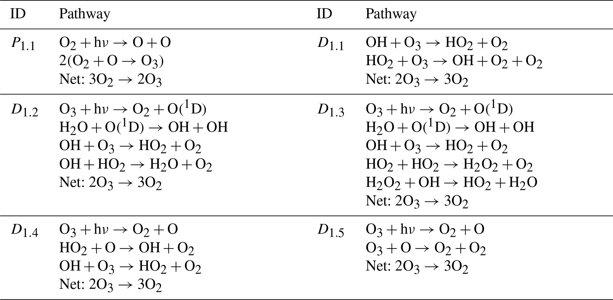
The construction of chemical pathways is essential to understand the results of photochemical models. These models typically represent hundreds of reactions producing and destroying chemical species within the atmosphere (see, for example, Hu et al., 2012; Tsai et al., 2017; Wogan et al., 2022). The interaction of these reactions makes it difficult to attribute the production or destruction of a species to a single reaction. Instead, to understand the mechanisms that affect the concentration of a species, it is necessary to construct pathways. A pathway is a sequence of reactions that interact with each other to produce, destroy, or recycle a species. For example, stratospheric ozone destruction is explained in terms of pathways that catalyze O₃ destruction (Lary, 1997). One of these pathways involves the reaction of O₃ with chlorine species (Molina and Rowland, 1974):

$$\begin{array}{}\text{(ClO pathway)}& \begin{array}{rl}& {\mathrm{O}}_{\mathrm{3}}+\mathrm{h}\mathit{\nu }\to {\mathrm{O}}_{\mathrm{2}}+\mathrm{O}\\ & \mathrm{Cl}+{\mathrm{O}}_{\mathrm{3}}\to \mathrm{ClO}+{\mathrm{O}}_{\mathrm{2}}\\ & \mathrm{ClO}+\mathrm{O}\to \mathrm{Cl}+\mathrm{O}\mathrm{2}\\ & \text{Net: }\mathrm{2}{\mathrm{O}}_{\mathrm{3}}\to \mathrm{3}{\mathrm{O}}_{\mathrm{2}}\end{array}\end{array}$$

This ozone-destroying pathway has three reactions, and its net effect is to convert two O₃ molecules into three O₂ molecules.

Several methods can help understand the results of photochemical models. For example, sensitivity analyses can constrain uncertainties in reaction rate constants and provide information on how variable the results of a model are when the reaction rates are perturbed (Turányi and Tomlin, 2014). Wiring diagrams can help understand the flow of molecules in a reaction system (Fishtik et al., 2006; Androulakis, 2006). However, these methods can not give quantitative information about the chains of reactions responsible for the production or destruction of a species in a chemical model. To understand these chemical mechanisms, it is necessary to construct pathways.

Chemical pathways are usually constructed manually and empirically, tracking and connecting reactions important for the production or destruction of a species of interest. However, the manual construction of pathways can not give a quantitative estimate of how important a pathway is for the production or destruction of a species relative to other pathways. Also, the manual construction of pathways has reproducibility limitations. Alternatively, pathways can be automatically constructed using algorithms (Milner, 1964; Schuster and Schuster, 1993; Clarke, 1988; Lehmann, 2002, 2004).

One of the most commonly used algorithms to construct pathways is the “Pathway analysis program” created by Lehmann (2004). This algorithm can automatically construct all the significant pathways in a reaction system and calculate the contribution of each pathway to the production and destruction of a species of interest. The “Pathway analysis program” has been used in several studies to gain a better understanding of atmospheric chemistry models (Grenfell et al., 2006; Verronen et al., 2011; Stock et al., 2012a, b; Verronen and Lehmann, 2013; Stock et al., 2017; Gebauer et al., 2017).

In this paper, we describe the development of Chempath, an open-source Python re-implementation of Lehmann's (2004) algorithm for analysis of photochemical models. We aim to contribute this open-source pathway analysis program to enhance the applicability of this algorithm to photochemical models and to enhance the replicability of chemical pathway construction. Our implementation is based on the description of the algorithm in Lehmann (2004). However, there is one difference between Chempath and the Lehmann (2004) algorithm. Our implementation does not include the balance of concentration changes and reaction rates that Lehmann's algorithm uses to eliminate imbalances due to numerical errors. Instead, Chempath requires input information about these imbalances to quantify the contributions of numerical errors to the production and destruction of a species.

We demonstrate how to apply this algorithm to a simple box model and to the one-dimensional photochemical model photochem (Wogan et al., 2023, https://github.com/Nicholaswogan/photochem, last access: 1 May 2025). Photochem is an updated version of Photochempy (Wogan, 2023a), a model that has been used for exoplanet and early-Earth photochemical studies (Wogan et al., 2022; Thompson et al., 2022; Garduno Ruiz et al., 2023, 2024). This model originates from Atmos, a photochemical model extensively used to investigate photochemistry in exoplanet and past atmospheres (see for example Kasting et al., 1979; Kasting and Donahue, 1980; Segura et al., 2005; Zahnle et al., 2006; Claire et al., 2014; Arney et al., 2016).

The structure of the paper is as follows. In Sect. 2, we review the Lehmann (2004) algorithm via a simple example. In Sect. 3, we describe how we implemented Chempath. In Sect. 4, we demonstrate how to apply Chempath to a simple box model and to the one-dimensional photochemical model photochem.

2 Algorithm review, a simple example

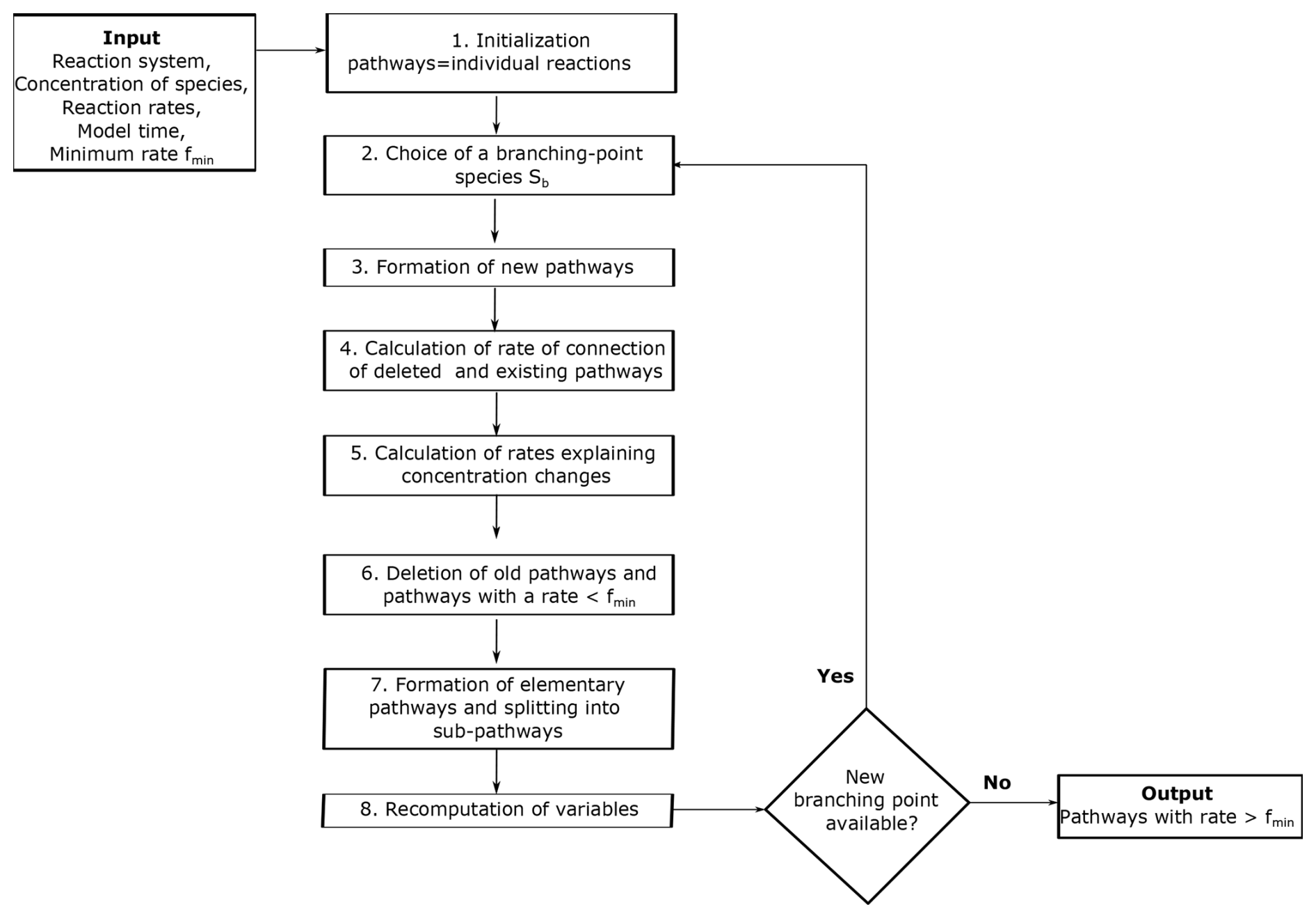
Here we provide a summary of the pathway analysis program presented in Lehmann (2004), using a simple example to explain each step of the algorithm (see the original paper for further details). The pathway analysis program forms pathways by the iterative connection of reactions through branching-point species (Fig. 1). A branching-point species is one that is used to connect reactions that produce the species to reactions that destroy it. For example, the reaction $\mathrm{Cl}+{\mathrm{O}}_{\mathrm{3}}\to \mathrm{ClO}+{\mathrm{O}}_{\mathrm{2}}$ can be connected to the reaction $\mathrm{ClO}+\mathrm{O}\to \mathrm{Cl}+{\mathrm{O}}_{\mathrm{2}}$ through the branching-point species ClO.

Figure 1 The Pathway Analysis Program algorithm. For a full description of the algorithm, see Lehmann (2004).

The example we use to demonstrate the algorithm consists of five reactions between six species involving hydrogen oxide radicals. The reactions are

$$\begin{array}{}\text{(R1)}& {\displaystyle }{\mathrm{H}}_{\mathrm{2}}{\mathrm{O}}_{\mathrm{2}}+\mathrm{OH}\to {\mathrm{HO}}_{\mathrm{2}}+{\mathrm{H}}_{\mathrm{2}}\mathrm{O},\text{with rate}=\mathrm{0.1}\mathrm{ppb}{\mathrm{h}}^{-\mathrm{1}}\text{(R2)}& {\displaystyle }\mathrm{OH}+\mathrm{OH}\to {\mathrm{H}}_{\mathrm{2}}{\mathrm{O}}_{\mathrm{2}},\text{with rate}=\mathrm{0.6}\mathrm{ppb}{\mathrm{h}}^{-\mathrm{1}}\text{(R3)}& {\displaystyle }{\mathrm{H}}_{\mathrm{2}}{\mathrm{O}}_{\mathrm{2}}+\mathrm{O}\to \mathrm{OH}+{\mathrm{HO}}_{\mathrm{2}},\text{with rate}=\mathrm{1}\mathrm{ppb}{\mathrm{h}}^{-\mathrm{1}}\text{(R4)}& {\displaystyle }{\mathrm{HO}}_{\mathrm{2}}+\mathrm{h}\mathit{\nu }\to \mathrm{OH}+\mathrm{O},\text{with rate}=\mathrm{0.5}\mathrm{ppb}{\mathrm{h}}^{-\mathrm{1}}\text{(R5)}& {\displaystyle }{\mathrm{HO}}_{\mathrm{2}}+\mathrm{O}\to \mathrm{OH}+{\mathrm{O}}_{\mathrm{2}},\text{with rate}=\mathrm{1}\mathrm{ppb}{\mathrm{h}}^{-\mathrm{1}},\end{array}$$

and the species are

$$\begin{array}{}\text{(S1)}& {\displaystyle }{\mathrm{H}}_{\mathrm{2}}{\mathrm{O}}_{\mathrm{2}},\text{with a mixing ratio of 2\hspace{0.17em}ppm}\text{(S2)}& {\displaystyle }\mathrm{OH},\text{with a mixing ratio of 3\hspace{0.17em}ppm}\text{(S3)}& {\displaystyle }{\mathrm{HO}}_{\mathrm{2}},\text{with a mixing ratio of 2\hspace{0.17em}ppm}\text{(S4)}& {\displaystyle }{\mathrm{H}}_{\mathrm{2}}\mathrm{O},\text{with a mixing ratio of 10\hspace{0.17em}ppm}\text{(S5)}& {\displaystyle }\mathrm{O},\text{with a mixing ratio of 1.5\hspace{0.17em}ppm}\text{(S6)}& {\displaystyle }{\mathrm{O}}_{\mathrm{2}},\text{with a mixing ratio of 100\hspace{0.17em}ppm}.\end{array}$$

We arbitrarily select these rates and mixing ratios for this example. Assuming that this reaction system is run for 1 h, the production and destruction by the reactions result in mixing ratio changes of −0.5, 1.2, −0.4, 0.1, −1.5, and 1 ppb for each species, respectively. In the next sections, we will identify the combination of reactions that is the most important to explain the OH mixing ratio change.

2.1 Assumptions and definitions

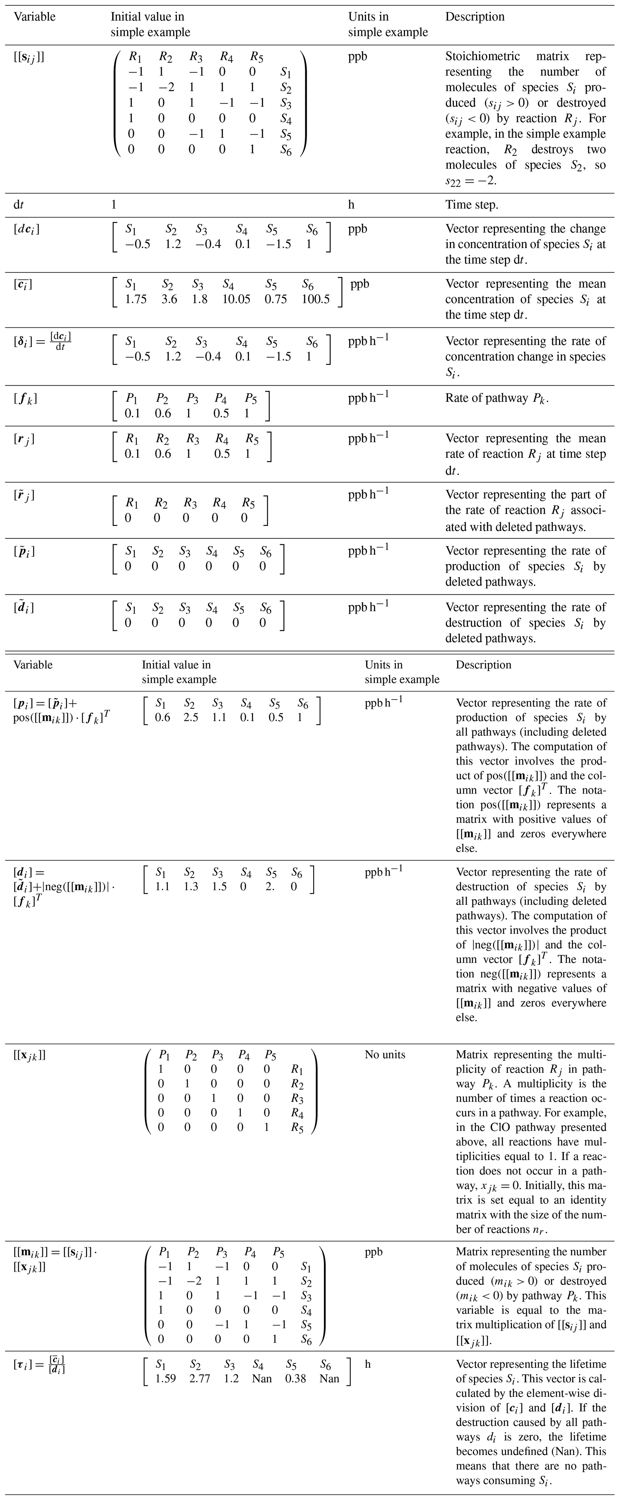
The algorithm uses the variables listed in Table 1 to construct pathways. We use two square brackets to denote variables that represent matrices (for example [[s_ij]]), and one to denote vectors (for example [c_i]). We denote the elements of a vector or matrix with sub-indexes. For example, c_i is the ith element of the vector [c_i], and s_ij is the element of [[s_ij]] located in the ith row and jth column. Similarly, [s_3j] denotes the third row of the matrix [[s_ij]]. We also use the notation pos([[x]]) to refer to a function that makes the negative values of a vector or matrix zero. Similarly, neg([[x]]) is a function that makes the positive values of a vector or matrix zero.

In large reaction systems, it might not be possible to construct all the pathways of the system because the number of pathways could be computationally unmanageable. The algorithm includes the option to delete unimportant pathways to avoid the construction of an unmanageable number of pathways and to reduce the computation time. However, the algorithm includes variables to keep track of the rates of these deleted pathways.

Table 1 Variables used in the pathway analysis algorithm and their initial values in the simple example used to explain the algorithm.

The algorithm assumes that the reactions are unidirectional and that the user splits the reversible reactions into their forward and backward components. It is also assumed that mass is conserved in the chemical model analyzed, and the reactions produce the exact number of molecules to explain the concentration changes:

$$\begin{array}{}\text{(1)}& \left[\mathrm{d}{\mathit{c}}_i\right]=\left[\right[{\mathbf{s}}_{ij}\left]\right]\cdot [{\mathit{r}}_j{]}^T\mathrm{d}t.\end{array}$$

This expression involves the product of [[s_ij]] and the column vector [r_j]^T. For example, in our simple example, we can verify that this condition is satisfied:

$$\begin{array}{}\text{(2)}& \begin{array}{rl}\left[\mathrm{d}{\mathit{c}}_i\right]& =\left(\begin{array}{ccccc}& & \left[\right[{\mathbf{s}}_{ij}\left]\right]& & \\ -\mathrm{1}& \mathrm{1}& -\mathrm{1}& \mathrm{0}& \mathrm{0}\\ -\mathrm{1}& -\mathrm{2}& \mathrm{1}& \mathrm{1}& \mathrm{1}\\ \mathrm{1}& \mathrm{0}& \mathrm{1}& -\mathrm{1}& -\mathrm{1}\\ \mathrm{1}& \mathrm{0}& \mathrm{0}& \mathrm{0}& \mathrm{0}\\ \mathrm{0}& \mathrm{0}& -\mathrm{1}& \mathrm{1}& -\mathrm{1}\\ \mathrm{0}& \mathrm{0}& \mathrm{0}& \mathrm{0}& \mathrm{1}\end{array}\right)\left(\begin{array}{c}[{\mathit{r}}_j{]}^T\\ \mathrm{0.1}\\ \mathrm{0.6}\\ \mathrm{1}\\ \mathrm{0.5}\\ \mathrm{1}\end{array}\right)\text{ppb}{\text{h}}^{-\mathrm{1}}\\ & \cdot \mathrm{1}\text{h}=\left[\begin{array}{cccccc}{S}_{\mathrm{1}}& S_{\mathrm{2}}& S_{\mathrm{3}}& S_{\mathrm{4}}& S_{\mathrm{5}}& S_{\mathrm{6}}\\ -\mathrm{0.5}& \mathrm{1.2}& -\mathrm{0.4}& \mathrm{0.1}& -\mathrm{1.5}& \mathrm{1}\end{array}\right]\text{ppb}.\end{array}\end{array}$$

2.2 Algorithm initialization

The algorithm requires four inputs from a chemical kinetics model: the species concentrations and the model time at two consecutive model times t and t+dt, the mean reaction rates at the time step dt, and the reaction system with n_r reactions between n_s species. We use the model times at which the solver obtains a solution for the system of equations. The user can also input a minimum rate of pathways f_min. With these inputs, the algorithm determines all pathways with a rate >f_min. In the simple example, we will use a minimum rate of pathways f_min=0.05 ppb h⁻¹.

The algorithm uses the input information to initialize the variables listed in Table 1. At first, each pathway is considered to have only one reaction, and the matrix [[x_jk]] is initialized as an identity matrix with the same size as the number of reactions. This means that initially pathway P₁ only contains reaction R₁, pathway P₂ only contains reaction R₂, etc. The rates of the pathways are initialized with the rates of the reactions: [f_j]=[r_j]. The variables $\left[{\stackrel{\mathrm{̃}}{\mathit{r}}}_j\right]$, $\left[{\stackrel{\mathrm{̃}}{\mathit{p}}}_i\right]$, and $\left[{\stackrel{\mathrm{̃}}{\mathit{d}}}_i\right]$ that store rates associated with deleted pathways are initialized as arrays of zeros.

2.3 Choice of branching-point species

Once the algorithm has been initialized, the next step is to choose a branching-point species S_b to start constructing pathways. Species with shorter lifetimes are selected as branching-point species first because a short lifetime is associated with fast consumption by reactions. The algorithm forms new pathways through the iterative connection of previously formed pathways through branching-point species until there are no more branching-point species left (Fig. 1). A species can be a branching-point species only once. To find pathways that destroy or produce a specific species of interest, the species itself is not used as a branching point. Otherwise, the pathways producing and consuming this species would be connected. Sometimes it is useful to treat some species as inert or long-lived and to not considering them branching-point species. For example, in the atmosphere, N₂ is long-lived and inert, so it could be not considered a branching point.

In the simple example where we are investigating the change in OH, we will treat H₂O and O₂ as a long-lived inert species, not considering them to be branching points. The species with the shortest lifetime is O (τ₅=0.38 h), so this species is the first branching point.

2.4 Formation of new pathways and rate calculations

The algorithm forms new pathways connecting all previously formed pathways that produce a branching-point species S_b to all pathways that destroy S_b. The connections are made ensuring that the new pathways do not produce or destroy the branching-point species S_b. If a pathway P_k produces m_bk molecules of the branching-point species S_b and a pathway P_l destroys m_bl molecules of S_b, the connection of these pathways forms a new pathway P_n with multiplicities:

$$\begin{array}{}\text{(3)}& \left[{\mathit{x}}_{jn}\right]=\left|m_{\mathrm{bl}}\right|\left[{\mathbf{x}}_{jk}\right]+m_{\mathrm{bk}}\left[{\mathit{x}}_{jl}\right],\end{array}$$

where k and l are the indexes of the pathways producing and destroying S_b, and b is the index of the species S_b. The rate f_n of the new pathway P_n is calculated by multiplying the rates of the producing (f_k) and destroying (f_l) pathways and dividing by the maximum of the rate of production and destruction of the branching-point species caused by all pathways:

$$\begin{array}{}\text{(4)}& f_{\mathrm{n}}={\displaystyle \frac{f_k{f}_l}{max(p_{\mathrm{b}},d_{\mathrm{b}})}},\end{array}$$

where k and l are the indexes of the pathways producing and destroying the branching-point species S_b, and b is the index of the branching-point species. This equation is derived by calculating the rate at which the molecules of S_b formed by P_k are destroyed by P_l (see Lehmann, 2004, for the derivation). One can think of Eq. (4) as distributing the rate of a pathway to new pathways using the probability that a molecule produced (or consumed) by one pathway is consumed (or produced) by another pathway. For example, if the change in concentration of the branching-point species is dc_b>0, then the chemical production is greater than the chemical destruction (p_b>d_b), and Eq. (4) takes the form $f_{\mathrm{n}}=\frac{{\mathit{f}}_k{f}_l}{p_{\mathrm{b}}}$. The ratio $\mathit{\pi }=\frac{{\mathit{f}}_k}{p_{\mathrm{b}}}$ can be interpreted as the probability that a molecule of the branching-point species is produced by the pathway P_k. Since the pathway P_l is going to be connected to all pathways P_k producing S_b, and the sum of the probabilities π over all pathways producing the branching-point species S_b is equal to 1, the rate f_l is going to be completely distributed to the new pathways.

The multiplicities [x_jn] of the new pathway are divided by their greatest common divisor g to keep them as simple as possible. The rate of the new pathway is multiplied by g to avoid altering the number of molecules that the new pathway produces or destroys. The new pathway and its rate are appended to [[x_jk]] and [f_k], respectively.

In the simple example, there are two pathways destroying the branching-point species O (P₃ and P₅) and one pathway producing it (P₄). The connection of these pathways will result in two new pathways. For example, the pathway P₃ destroys one O molecule ($m_{\mathrm{53}}=-\mathrm{1}$), and the pathway P₄ produces one O molecule (m₅₄=1), so the connection of these pathways results in a new pathway with multiplicities:

$$\begin{array}{}\text{(5)}& \begin{array}{rl}\left[{\mathit{x}}_{jn}\right]& =\left|m_{\mathrm{53}}\right|\left[{\mathit{x}}_{j\mathrm{4}}\right]+m_{\mathrm{54}}\left[{\mathit{x}}_{j\mathrm{3}}\right]=[\mathrm{0},\mathrm{0},\mathrm{0},\mathrm{1},\mathrm{0}]\\ & +[\mathrm{0},\mathrm{0},\mathrm{1},\mathrm{0},\mathrm{0}]=[\mathrm{0},\mathrm{0},\mathrm{1},\mathrm{1},\mathrm{0}].\end{array}\end{array}$$

The rate of this new pathway is

$$\begin{array}{}\text{(6)}& \begin{array}{rl}{f}_{\mathrm{n}}& ={\displaystyle \frac{f_{\mathrm{4}}{f}_{\mathrm{3}}}{max(p_{\mathrm{5}},d_{\mathrm{5}})}}={\displaystyle \frac{\mathrm{0.5}{\text{ppb\hspace{0.17em}h}}^{-\mathrm{1}}\cdot \mathrm{1}{\text{ppb\hspace{0.17em}h}}^{-\mathrm{1}}}{\mathrm{2}{\text{ppb\hspace{0.17em}h}}^{-\mathrm{1}}}}\\ & =\mathrm{0.25}{\text{ppb\hspace{0.17em}h}}^{-\mathrm{1}}.\end{array}\end{array}$$

After forming all new pathways at the branching-point species O, the multiplicities [[x_jk]] and the pathway rates [f_k] will have the following form:

$$\begin{array}{}\text{(7)}& \begin{array}{rl}& \left[\right[{\mathbf{x}}_{jk}\left]\right]=\left(\begin{array}{ccccccc}{P}_{\mathrm{1}}& P_{\mathrm{2}}& P_{\mathrm{3}}& P_{\mathrm{4}}& P_{\mathrm{5}}& P_{\mathrm{6}}& P_{\mathrm{7}}\\ \mathrm{1}& \mathrm{0}& \mathrm{0}& \mathrm{0}& \mathrm{0}& \mathrm{0}& \mathrm{0}& R_{\mathrm{1}}\\ \mathrm{0}& \mathrm{1}& \mathrm{0}& \mathrm{0}& \mathrm{0}& \mathrm{0}& \mathrm{0}& R_{\mathrm{2}}\\ \mathrm{0}& \mathrm{0}& \mathrm{1}& \mathrm{0}& \mathrm{0}& \mathrm{1}& \mathrm{0}& R_{\mathrm{3}}\\ \mathrm{0}& \mathrm{0}& \mathrm{0}& \mathrm{1}& \mathrm{0}& \mathrm{1}& \mathrm{1}& R_{\mathrm{4}}\\ \mathrm{0}& \mathrm{0}& \mathrm{0}& \mathrm{0}& \mathrm{1}& \mathrm{0}& \mathrm{1}& R_{\mathrm{5}}\end{array}\right)\\ & \left[{\mathit{f}}_k\right]=\left[\begin{array}{ccccccc}{P}_{\mathrm{1}}& P_{\mathrm{2}}& P_{\mathrm{3}}& P_{\mathrm{4}}& P_{\mathrm{5}}& P_{\mathrm{6}}& P_{\mathrm{7}}\\ \mathrm{0.1}& \mathrm{0.6}& \mathrm{1}& \mathrm{0.5}& \mathrm{1}& \mathrm{0.25}& \mathrm{0.25}\end{array}\right]{\text{ppb\hspace{0.17em}h}}^{-\mathrm{1}}.\end{array}\end{array}$$

We can think of a column in [[x_jk]] as a pathway. For example, the pathway that we formed before (P₆) is located in the sixth column of the matrix [[x_jk]] in Eq. (7) and contains one R₃ reaction and one R₄ reaction:

$$\begin{array}{}\text{(P6)}& \begin{array}{rl}& {\mathrm{H}}_{\mathrm{2}}{\mathrm{O}}_{\mathrm{2}}+\mathrm{O}\to \mathrm{OH}+{\mathrm{HO}}_{\mathrm{2}}\\ & \mathrm{HO}\mathrm{2}+\mathrm{h}\mathit{\nu }\to \mathrm{OH}+\mathrm{O}\\ & \text{Net: }{\mathrm{H}}_{\mathrm{2}}{\mathrm{O}}_{\mathrm{2}}\to \mathrm{2}\mathrm{OH}.\end{array}\end{array}$$

2.5 Calculation of the rate of connection of deleted and existing pathways

In this step, the algorithm calculates the rates of connection of deleted pathways to existing pathways. Pathways with a rate lower than f_min will be deleted in a subsequent step (see Sect. 2.7). In the first iteration of the algorithm, there are no deleted pathways, but in other iterations, some pathways can be deleted by this point. In that case, the deleted pathways would not be connected to existing pathways. However, the algorithm keeps track of the rates of production and destruction of the branching-point species S_b that would have been computed in these connections. The deleted pathways produce the branching-point species S_b at a rate ${\stackrel{\mathrm{̃}}{p}}_{\mathrm{b}}$, so according to Eq. (4), the rate of the connection of deleted pathways that produces S_b to an existing pathway P_e that destroys S_b is

$$\begin{array}{}\text{(8)}& {\stackrel{\mathrm{̃}}{f}}_{\mathrm{e}}={\displaystyle \frac{f_{\mathrm{e}}{\stackrel{\mathrm{̃}}{p}}_{\mathrm{b}}}{max(p_{\mathrm{b}},d_{\mathrm{b}})}},\end{array}$$

where e represents the index of the pathway that destroys the branching-point species S_b. Similarly, deleted pathways consuming S_b at a rate ${\stackrel{\mathrm{̃}}{d}}_{\mathrm{b}}$ would have been connected to an existing pathway P_e, producing S_b at a rate of

$$\begin{array}{}\text{(9)}& {\stackrel{\mathrm{̃}}{f}}_{\mathrm{e}}={\displaystyle \frac{f_{\mathrm{e}}{\stackrel{\mathrm{̃}}{d}}_{\mathrm{b}}}{max(p_{\mathrm{b}},d_{\mathrm{b}})}},\end{array}$$

where e represents the index of the pathway that produces S_b. This rate is added to the variables $\left[{\stackrel{\mathrm{̃}}{\mathit{r}}}_j\right]$, $\left[{\stackrel{\mathrm{̃}}{\mathit{p}}}_i\right]$, and $\left[{\stackrel{\mathrm{̃}}{\mathit{d}}}_i\right]$ that store rates associated with deleted pathways:

$$\begin{array}{}\text{(10)}& \begin{array}{rl}& \left[{\stackrel{\mathrm{̃}}{\mathit{r}}}_j\right]=\left[{\stackrel{\mathrm{̃}}{\mathit{r}}}_j\right]+\left[{\mathit{x}}_{je}\right]\cdot {\stackrel{\mathrm{̃}}{f}}_{\mathrm{e}}\\ & \left[{\stackrel{\mathrm{̃}}{\mathit{p}}}_i\right]=\left[{\stackrel{\mathrm{̃}}{\mathit{p}}}_i\right]+\text{pos}\left(\right[{\mathit{m}}_{ie}\left]\right)\cdot {\stackrel{\mathrm{̃}}{f}}_{\mathrm{e}}\\ & \left[{\stackrel{\mathrm{̃}}{\mathit{d}}}_i\right]=\left[{\stackrel{\mathrm{̃}}{\mathit{d}}}_i\right]+\left|\text{neg}\right(\left[{\mathit{m}}_{ie}\right]\left)\right|\cdot {\stackrel{\mathrm{̃}}{f}}_{\mathrm{e}},\end{array}\end{array}$$

where e= index of pathway producing or destroying the branching-point species S_b. These operations are repeated for all existing pathways producing and destroying the branching-point species. In the simple example, there are no deleted pathways yet, so ${\stackrel{\mathrm{̃}}{f}}_{\mathrm{e}}=\mathrm{0}$.

2.6 Calculation of rates explaining concentration changes

In this step, the algorithm redefines the rates of the pathways that contribute to the concentration change in the branching-point species S_b. If dc_b>0, the pathways that produce molecules of the branching-point species S_b contribute to its concentration change dc_b. Similarly, if dc_b<0, the pathways that destroy molecules of the branching-point species S_b contribute to its concentration change dc_b. The algorithm redefines the rate f_k of pathways contributing to the concentration change in the branching-point species, keeping the fraction $\widehat{f_k}$ of f_k that contributes to the concentration change dc_b. This fraction is calculated by multiplying the rate f_k by the absolute value of the rate of concentration change in the branching-point species δ_b and dividing by the maximum of the production and destruction of the branching-point species caused by all pathways:

$$\begin{array}{}\text{(11)}& {\widehat{f}}_k={\displaystyle \frac{f_k\left|{\mathit{\delta }}_{\mathrm{b}}\right|}{max(p_{\mathrm{b}},d_{\mathrm{b}})}},\end{array}$$

where k=the index of the pathway producing or destroying S_b, and b is the index of the branching-point species S_b. This rate is derived by calculating the probability that a molecule of S_b produced or destroyed by a pathway contributes to the concentration change in the branching-point species dc_b (see Lehmann, 2004, for the derivation). If dc_b=0, there is no redefinition of rates.

In the simple example, the branching-point species O has a concentration change d$c_{\mathrm{5}}=-\mathrm{1.5}\text{ppb}$. Since dc₅<0, we will redefine the rates of the pathways that destroy O because they contribute to the concentration change dc₅. For example, the pathway P₃ has a single reaction destroying O at a rate of 1 ppb h⁻¹. The part of this rate that contributes to the O concentration change is

$$\begin{array}{}\text{(12)}& \begin{array}{rl}\widehat{f_{\mathrm{3}}}& ={\displaystyle \frac{f_{\mathrm{3}}\left|{\mathit{\delta }}_{\mathrm{5}}\right|}{max(p_{\mathrm{5}},d_{\mathrm{5}})}}={\displaystyle \frac{\mathrm{1}{\text{ppb\hspace{0.17em}h}}^{-\mathrm{1}}\cdot \mathrm{1.5}{\text{ppb\hspace{0.17em}h}}^{-\mathrm{1}}}{\mathrm{2}{\text{ppb\hspace{0.17em}h}}^{-\mathrm{1}}}}\\ & =\mathrm{0.75}{\text{ppb\hspace{0.17em}h}}^{-\mathrm{1}}.\end{array}\end{array}$$

After all the rates of the pathways destroying S_b are redefined, [f_k] has the form

$$\begin{array}{}\text{(13)}& \left[{\mathit{f}}_k\right]=\left[\begin{array}{ccccccc}{P}_{\mathrm{1}}& P_{\mathrm{2}}& P_{\mathrm{3}}& P_{\mathrm{4}}& P_{\mathrm{5}}& P_{\mathrm{6}}& P_{\mathrm{7}}\\ \mathrm{0.1}& \mathrm{0.6}& \mathrm{0.75}& \mathrm{0.5}& \mathrm{0.75}& \mathrm{0.25}& \mathrm{0.25}\end{array}\right]{\text{ppb\hspace{0.17em}h}}^{-\mathrm{1}}.\end{array}$$

2.7 Deletion of old pathways and pathways with a rate <f_min

After a pathway producing the branching-point species S_b has been connected to all pathways destroying S_b, it is eliminated from the matrix [[x_jk]] if it does not contribute to the concentration change dc_b. If dc_b>0, the pathways that destroy the branching-point species are deleted. If dc_b<0, the pathways that produce the branching-point species are deleted, and if dc_b=0, the pathways that both produce and destroy the branching-point species are deleted.

In the simple example, dc₅<0, so pathways P₃ and P₅ that were used to form new pathways will not be deleted because they destroy molecules of the branching-point species O, contributing to its concentration change. However, the pathway P₄ does not contribute to dc₅, so it is deleted.

The algorithm also deletes pathways with a rate <f_min to avoid constructing an unmanageable number of pathways and to reduce the computing time. If a pathway has a rate f_q<f_min, it is deleted from the matrix [[x_jk]], and the variables $\left[{\stackrel{\mathrm{̃}}{\mathit{r}}}_j\right]$, $\left[{\stackrel{\mathrm{̃}}{\mathit{p}}}_i\right]$, and $\left[{\stackrel{\mathrm{̃}}{\mathit{d}}}_i\right]$ are updated according to

$$\begin{array}{}\text{(14)}& \begin{array}{rl}& \left[{\stackrel{\mathrm{̃}}{\mathit{r}}}_j\right]=\left[{\stackrel{\mathrm{̃}}{\mathit{r}}}_j\right]+\left[{\mathit{x}}_{jq}\right]\cdot f_q\\ & \left[{\stackrel{\mathrm{̃}}{\mathit{p}}}_i\right]=\left[{\stackrel{\mathrm{̃}}{\mathit{p}}}_i\right]+\text{pos}\left(\right[{\mathit{m}}_{iq}\left]\right)\cdot f_q\\ & \left[{\stackrel{\mathrm{̃}}{\mathit{d}}}_i\right]=\left[{\stackrel{\mathrm{̃}}{\mathit{d}}}_i\right]+\left|\text{neg}\right(\left[{\mathit{m}}_{iq}\right]\left)\right|\cdot f_q,\end{array}\end{array}$$

where $q=\text{index of the pathway with rate}<f_{\text{min}}$. These operations are repeated for all pathways with rate <f_min. The rates of these pathways are also deleted from [f_k].

In the simple example, none of the pathways have a rate <f_min, so there is no deletion of pathways in this first iteration. See Sect. 2.10 to see an example of how pathways with a rate <f_min are deleted. After this step, the multiplicities [[x_jk]] and the pathway rates [f_k] will have the following form:

$$\begin{array}{}\text{(15)}& \begin{array}{rl}& \left[\right[{\mathbf{x}}_{jk}\left]\right]=\left(\begin{array}{cccccc}{P}_{\mathrm{1}}& P_{\mathrm{2}}& P_{\mathrm{3}}& P_{\mathrm{4}}& P_{\mathrm{5}}& P_{\mathrm{6}}\\ \mathrm{1}& \mathrm{0}& \mathrm{0}& \mathrm{0}& \mathrm{0}& \mathrm{0}& R_{\mathrm{1}}\\ \mathrm{0}& \mathrm{1}& \mathrm{0}& \mathrm{0}& \mathrm{0}& \mathrm{0}& R_{\mathrm{2}}\\ \mathrm{0}& \mathrm{0}& \mathrm{1}& \mathrm{0}& \mathrm{1}& \mathrm{0}& R_{\mathrm{3}}\\ \mathrm{0}& \mathrm{0}& \mathrm{0}& \mathrm{0}& \mathrm{1}& \mathrm{1}& R_{\mathrm{4}}\\ \mathrm{0}& \mathrm{0}& \mathrm{0}& \mathrm{1}& \mathrm{0}& \mathrm{1}& R_{\mathrm{5}}\end{array}\right)\\ & \left[{\mathit{f}}_k\right]=\left[\begin{array}{cccccc}{P}_{\mathrm{1}}& P_{\mathrm{2}}& P_{\mathrm{3}}& P_{\mathrm{4}}& P_{\mathrm{5}}& P_{\mathrm{6}}\\ \mathrm{0.1}& \mathrm{0.6}& \mathrm{0.75}& \mathrm{0.75}& \mathrm{0.25}& \mathrm{0.25}\end{array}\right]{\text{ppb\hspace{0.17em}h}}^{-\mathrm{1}}.\end{array}\end{array}$$

Note that when pathways are deleted from the matrix [[x_jk]], there is a redefinition of pathways. For example, since pathway P₄ was deleted, now there is a new pathway P₄ that corresponds to the fourth column of [[x_jk]] in Eq. (15).

2.8 Formation of elementary pathways and splitting into sub-pathways

The steps above can produce pathways with a large and unnecessary number of reactions. The algorithm splits these complex pathways into shorter, simpler pathways. The first step in this process is to find the elementary sub-pathways of a complex pathway. A pathway P_s is a sub-pathway of a pathway P_c if all the reactions in P_s are in P_c. Elementary pathways do not have sub-pathways. The algorithm finds the elementary sub-pathways of a pathway P_c by forming new pathways with the reactions contained in P_c and keeping only the elementary pathways (see Lehmann, 2004, for a full description of this process). If a pathway P_c with multiplicities [x_jc] has n_e elementary sub-pathways with multiplicities $\left[\right[{\mathbf{x}}_{je}^{\prime }\left]\right]$, the algorithm splits [x_jc] into the sub-pathways $\left[\right[{\mathbf{x}}_{je}^{\prime }\left]\right]$, finding weights [w_e] that fulfill the following equation:

$$\begin{array}{}\text{(16)}& \begin{array}{rl}\left[{\mathit{x}}_{jc}\right]& =\left[\right[{\mathbf{x}}_{je}^{\prime }]{]}^T\cdot [{\mathit{w}}_e],\text{ where }c=\text{ index of}\\ & \text{the pathway to be split.}\end{array}\end{array}$$

Equation (16) involves the matrix multiplication of $\left[\right[{\mathbf{x}}_{je}^{\prime }]{]}^T$ and the row vector [w_e]. In other words, the sum of the multiplicities of the sub-pathways multiplied by the weights must be equal to the multiplicities of the split pathway. The rate f_c of the pathway P_c is distributed to the sub-pathways using the weights [w_e]:

$$\begin{array}{}\text{(17)}& \begin{array}{rl}\left[{\mathit{f}}_{\mathrm{e}}\right]& =f_c\left[{\mathit{w}}_e\right],\text{ where }e=\mathrm{1}\mathrm{\dots }{n}_e,\text{ and }c=\text{index of}\\ & \text{the pathway to be split.}\end{array}\end{array}$$

After finding the sub-pathways, the algorithm deletes [x_jc] from [[x_jk]] and adds the multiplicities of the new sub-pathways $\left[\right[{\mathbf{x}}_{je}^{\prime }\left]\right]$ to [[x_jk]]. Similarly, the rate f_c is deleted, and the rates [f_e] are appended to [f_k]. If a sub-pathway already exists in the matrix [[x_jk]], its rate is added to the already-existing pathway.

As noted by Lehmann (2004), Eq. (16) can have multiple solutions, leading to slightly different results according to the solution that one chooses. However, these differences tend to be small, and the overall result of the algorithm is similar even when Eq. (16) has multiple solutions (Lehmann, 2004). Our implementation includes two options to solve Eq. (16). The first option uses Scipy's “lsq_linear” function, minimizing the expression

$$\begin{array}{}\text{(18)}& \mathrm{0.5}\left|\right|A\cdot x-b|{|}^{\mathrm{2}}\text{with constraints}\mathrm{0}\le x<\mathrm{\infty },\end{array}$$

where $\left|\right|x\left|\right|$ is the norm of x, $A=\left[\right[{\mathbf{x}}_{je}^{\prime }]{]}^T$, x=[w_e], and b=[x_jc]. When there are multiple solutions to Eq. (16), we choose the first solution found by the “lsq_linear” algorithm that minimizes Eq. (18). The second option to solve Eq. (16) implements the method proposed in Sect. 5.5.2 of Lehmann (2004). This method chooses the solution that produces more probable pathways, in the sense that this solution produces simpler pathways with higher rates compared to other solutions. Both methods of solving Eq. (16) produce similar results.

In the first iteration of the algorithm in the simple example, there are no pathways to split. See Sect. 2.10 for an example of how to split pathways into sub-pathways.

2.9 Re-computation of variables

The variables [[m_ik]], [p_i], and [d_i] are recomputed using the definitions presented in Table 1 to match the information from the new pathways formed in the above steps. This re-computation is done after deleting pathways and after splitting pathways into sub-pathways.

In the simple example, this re-computation results in the following values for [[m_ik]], [p_i], and [d_i]:

$$\begin{array}{}\text{(19)}& {\displaystyle }\begin{array}{rl}\left[\right[{\mathbf{m}}_{ik}\left]\right]& =\left(\begin{array}{ccccc}& & \left[\right[{\mathbf{s}}_{ij}\left]\right]& & \\ -\mathrm{1}& \mathrm{1}& -\mathrm{1}& \mathrm{0}& \mathrm{0}\\ -\mathrm{1}& -\mathrm{2}& \mathrm{1}& \mathrm{1}& \mathrm{1}\\ \mathrm{1}& \mathrm{0}& \mathrm{1}& -\mathrm{1}& -\mathrm{1}\\ \mathrm{1}& \mathrm{0}& \mathrm{0}& \mathrm{0}& \mathrm{0}\\ \mathrm{0}& \mathrm{0}& -\mathrm{1}& \mathrm{1}& -\mathrm{1}\\ \mathrm{0}& \mathrm{0}& \mathrm{0}& \mathrm{0}& \mathrm{1}\end{array}\right)\\ & \left(\begin{array}{cccccc}& & & \left[\right[{\mathbf{x}}_{jk}\left]\right]& & \\ \mathrm{1}& \mathrm{0}& \mathrm{0}& \mathrm{0}& \mathrm{0}& \mathrm{0}\\ \mathrm{0}& \mathrm{1}& \mathrm{0}& \mathrm{0}& \mathrm{0}& \mathrm{0}\\ \mathrm{0}& \mathrm{0}& \mathrm{1}& \mathrm{0}& \mathrm{1}& \mathrm{0}\\ \mathrm{0}& \mathrm{0}& \mathrm{0}& \mathrm{0}& \mathrm{1}& \mathrm{1}\\ \mathrm{0}& \mathrm{0}& \mathrm{0}& \mathrm{1}& \mathrm{0}& \mathrm{1}\end{array}\right)\\ & =\left(\begin{array}{cccccc}{P}_{\mathrm{1}}& P_{\mathrm{2}}& P_{\mathrm{3}}& P_{\mathrm{4}}& P_{\mathrm{5}}& P_{\mathrm{6}}\\ -\mathrm{1}& \mathrm{1}& -\mathrm{1}& \mathrm{0}& -\mathrm{1}& \mathrm{0}& S_{\mathrm{1}}\\ -\mathrm{1}& -\mathrm{2}& \mathrm{1}& \mathrm{1}& \mathrm{2}& \mathrm{2}& S_{\mathrm{2}}\\ \mathrm{1}& \mathrm{0}& \mathrm{1}& -\mathrm{1}& \mathrm{0}& -\mathrm{2}& S_{\mathrm{3}}\\ \mathrm{1}& \mathrm{0}& \mathrm{0}& \mathrm{0}& \mathrm{0}& \mathrm{0}& S_{\mathrm{4}}\\ \mathrm{0}& \mathrm{0}& -\mathrm{1}& -\mathrm{1}& \mathrm{0}& \mathrm{0}& S_{\mathrm{5}}\\ \mathrm{0}& \mathrm{0}& \mathrm{0}& \mathrm{1}& \mathrm{0}& \mathrm{1}& S_{\mathrm{6}}\end{array}\right)\end{array}\text{(20)}& {\displaystyle }\begin{array}{rl}\left[{\mathit{p}}_i\right]& =\left[\begin{array}{ccccc}& & \left[{\stackrel{\mathrm{̃}}{\mathit{p}}}_i\right]& & \\ \mathrm{0}& \mathrm{0}& \mathrm{0}& \mathrm{0}& \mathrm{0}\end{array}\right]\\ & +\left(\begin{array}{cccccc}& & & \text{pos}\left(\right[\left[{\mathbf{m}}_{ik}\right]\left]\right)& & \\ \mathrm{0}& \mathrm{1}& \mathrm{0}& \mathrm{0}& \mathrm{0}& \mathrm{0}\\ \mathrm{0}& \mathrm{0}& \mathrm{1}& \mathrm{1}& \mathrm{2}& \mathrm{2}\\ \mathrm{1}& \mathrm{0}& \mathrm{1}& \mathrm{0}& \mathrm{0}& \mathrm{0}\\ \mathrm{1}& \mathrm{0}& \mathrm{0}& \mathrm{0}& \mathrm{0}& \mathrm{0}\\ \mathrm{0}& \mathrm{0}& \mathrm{0}& \mathrm{0}& \mathrm{0}& \mathrm{0}\\ \mathrm{0}& \mathrm{0}& \mathrm{0}& \mathrm{1}& \mathrm{0}& \mathrm{1}\end{array}\right)\left[\begin{array}{c}\left[{\mathit{f}}_k\right]\\ \mathrm{0.1}\\ \mathrm{0.6}\\ \mathrm{0.75}\\ \mathrm{0.75}\\ \mathrm{0.25}\\ \mathrm{0.25}\end{array}\right]\\ & =\left[\begin{array}{cccccc}{S}_{\mathrm{1}}& S_{\mathrm{2}}& S_{\mathrm{3}}& S_{\mathrm{4}}& S_{\mathrm{5}}& S_{\mathrm{6}}\\ \mathrm{0.6}& \mathrm{2.5}& \mathrm{0.85}& \mathrm{0.1}& \mathrm{0}& \mathrm{1}\end{array}\right]{\text{ppb\hspace{0.17em}h}}^{-\mathrm{1}}\end{array}\text{(21)}& {\displaystyle }\begin{array}{rl}\left[{\mathit{d}}_i\right]& =\left[\begin{array}{ccccc}& & \left[{\stackrel{\mathrm{̃}}{\mathit{d}}}_i\right]& & \\ \mathrm{0}& \mathrm{0}& \mathrm{0}& \mathrm{0}& \mathrm{0}\end{array}\right]\\ & +\left(\begin{array}{cccccc}& & & \left|\text{neg}\right(\left[\right[{\mathbf{m}}_{ik}\left]\right]\left)\right|& & \\ \mathrm{1}& \mathrm{0}& \mathrm{1}& \mathrm{0}& \mathrm{1}& \mathrm{0}\\ \mathrm{1}& \mathrm{2}& \mathrm{0}& \mathrm{0}& \mathrm{0}& \mathrm{0}\\ \mathrm{0}& \mathrm{0}& \mathrm{0}& \mathrm{1}& \mathrm{0}& \mathrm{2}\\ \mathrm{0}& \mathrm{0}& \mathrm{0}& \mathrm{0}& \mathrm{0}& \mathrm{0}\\ \mathrm{0}& \mathrm{0}& \mathrm{1}& \mathrm{1}& \mathrm{0}& \mathrm{0}\\ \mathrm{0}& \mathrm{0}& \mathrm{0}& \mathrm{0}& \mathrm{0}& \mathrm{0}\end{array}\right)\left[\begin{array}{c}\left[{\mathit{f}}_k\right]\\ \mathrm{0.1}\\ \mathrm{0.6}\\ \mathrm{0.75}\\ \mathrm{0.75}\\ \mathrm{0.25}\\ \mathrm{0.25}\end{array}\right]\\ & =\left[\begin{array}{cccccc}{S}_{\mathrm{1}}& S_{\mathrm{2}}& S_{\mathrm{3}}& S_{\mathrm{4}}& S_{\mathrm{5}}& S_{\mathrm{6}}\\ \mathrm{1.1}& \mathrm{1.3}& \mathrm{1.25}& \mathrm{0}& \mathrm{1.5}& \mathrm{0}\end{array}\right]{\text{ppb\hspace{0.17em}h}}^{-\mathrm{1}}.\end{array}\end{array}$$

2.10 Second iteration in the simple example

After the first iteration at the branching-point species O in the simple example, we ended up with six pathways (Eq. 15). The species with the shortest lifetime with respect to these new pathways and the next branching-point species is HO₂ (S₃). Looking at the third row of [[m_ik]] in Eq. (19) ([m_3k]), we can see that pathways P₄ and P₆ destroy HO₂ and pathways P₁ and P₃ produce HO₂. The connection of these pathways will lead to the formation of four new pathways (Sect. 2.4). For example, by connecting pathways P₆ and P₃, we obtain a new pathway P_n with the following multiplicities and rate:

$$\begin{array}{}\text{(22)}& \begin{array}{rl}\left[{\mathit{x}}_{jn}\right]& =\left|m_{\mathrm{36}}\right|\left[{\mathit{x}}_{j\mathrm{3}}\right]+m_{\mathrm{33}}\left[{\mathit{x}}_{j\mathrm{6}}\right]=\mathrm{2}\cdot [\mathrm{0},\mathrm{0},\mathrm{1},\mathrm{0},\mathrm{0}]\\ & +\mathrm{1}\cdot [\mathrm{0},\mathrm{0},\mathrm{0},\mathrm{1},\mathrm{1}]=[\mathrm{0},\mathrm{0},\mathrm{2},\mathrm{1},\mathrm{1}]\\ & f_{\mathrm{n}}={\displaystyle \frac{f_{\mathrm{3}}{f}_{\mathrm{6}}}{max(p_{\mathrm{3}},d_{\mathrm{3}})}}={\displaystyle \frac{\mathrm{0.75}{\text{ppb\hspace{0.17em}h}}^{-\mathrm{1}}\cdot \mathrm{0.25}{\text{ppb\hspace{0.17em}h}}^{-\mathrm{1}}}{\mathrm{1.25}{\text{ppb\hspace{0.17em}h}}^{-\mathrm{1}}}}\\ & =\mathrm{0.15}{\text{ppb\hspace{0.17em}h}}^{-\mathrm{1}}.\end{array}\end{array}$$

Similarly, the combination of pathways P₁ and P₆ will result in a pathway P_m with multiplicities $\left[{\mathit{x}}_{jm}\right]=[\mathrm{2},\mathrm{0},\mathrm{0},\mathrm{1},\mathrm{1}]$ and a rate f_m=0.02 ppb h⁻¹. This pathway produces and destroys the number of molecules $\left[m_{im}\right]=[-\mathrm{2},\mathrm{0},\mathrm{0},\mathrm{2},\mathrm{0},\mathrm{1}]$.

At this point, there is no production or destruction of HO₂ by deleted pathways, so the rates of connection of existing pathways to deleted pathways is ${\stackrel{\mathrm{̃}}{f}}_{\mathrm{e}}=\mathrm{0}$ (Sect. 2.5). Since the concentration change in the branching-point species HO₂ is d$c_{\mathrm{3}}=-\mathrm{0.4}\text{ ppb}<\mathrm{0}$, the rates of the pathways destroying HO₂ are redefined to keep the fraction that contributes to dc₃ (Sect. 2.6), and the pathways that produce HO₂ are deleted because they do not contribute to dc₃ (Sect. 2.7).

The rate of the pathway P_m is lower than f_min, so this pathway will be deleted, and the variables that store the rates of the deleted pathways are updated using Eq. (14) (Sect. 2.7):

$$\begin{array}{}\text{(23)}& \begin{array}{rl}& \left[{\stackrel{\mathrm{̃}}{\mathit{r}}}_j\right]=\left[{\stackrel{\mathrm{̃}}{\mathit{r}}}_j\right]+\left[{\mathit{x}}_{jm}\right]\cdot f_m=[\mathrm{0},\mathrm{0},\mathrm{0},\mathrm{0},\mathrm{0}]+[\mathrm{2},\mathrm{0},\mathrm{0},\mathrm{1},\mathrm{1}]\\ & \cdot \mathrm{0.02}{\text{ppb\hspace{0.17em}h}}^{-\mathrm{1}}=[\mathrm{0.04},\mathrm{0},\mathrm{0},\mathrm{0.02},\mathrm{0.02}]{\text{ppb\hspace{0.17em}h}}^{-\mathrm{1}}\\ & \left[{\stackrel{\mathrm{̃}}{\mathit{p}}}_i\right]=\left[{\stackrel{\mathrm{̃}}{\mathit{p}}}_i\right]+\text{pos}\left(\right[{\mathit{m}}_{im}\left]\right)\cdot f_m=[\mathrm{0},\mathrm{0},\mathrm{0},\mathrm{0},\mathrm{0},\mathrm{0}]\\ & +[\mathrm{0},\mathrm{0},\mathrm{0},\mathrm{2},\mathrm{0},\mathrm{1}]\cdot \mathrm{0.02}{\text{ppb\hspace{0.17em}h}}^{-\mathrm{1}}\\ & =[\mathrm{0},\mathrm{0},\mathrm{0},\mathrm{0.04},\mathrm{0},\mathrm{0.02}]{\text{ppb\hspace{0.17em}h}}^{-\mathrm{1}}\\ & \left[{\stackrel{\mathrm{̃}}{\mathit{d}}}_i\right]=\left[{\stackrel{\mathrm{̃}}{\mathit{d}}}_i\right]+\text{neg}\left(\right[{\mathit{m}}_{im}\left]\right)\cdot f_m=[\mathrm{0},\mathrm{0},\mathrm{0},\mathrm{0},\mathrm{0},\mathrm{0}]\\ & +[\mathrm{2},\mathrm{0},\mathrm{0},\mathrm{0},\mathrm{0},\mathrm{0}]\cdot \mathrm{0.02}{\text{ppb\hspace{0.17em}h}}^{-\mathrm{1}}\\ & =[\mathrm{0.04},\mathrm{0},\mathrm{0},\mathrm{0},\mathrm{0},\mathrm{0}]{\text{ppb\hspace{0.17em}h}}^{-\mathrm{1}}.\end{array}\end{array}$$

The next step is to split the pathways into sub-pathways (Sect. 2.8). The pathway P_n formed above (Eq. 22) contains two R₃ reactions, one R₄ reaction, and one R₅ reaction:

$$\begin{array}{}\text{(Pn)}& \begin{array}{rl}& \mathrm{2}({\mathrm{H}}_{\mathrm{2}}{\mathrm{O}}_{\mathrm{2}}+\mathrm{O}\to \mathrm{OH}+{\mathrm{HO}}_{\mathrm{2}})\\ & {\mathrm{HO}}_{\mathrm{2}}+\mathrm{h}\mathit{\nu }\to \mathrm{OH}+\mathrm{O}\\ & {\mathrm{HO}}_{\mathrm{2}}+\mathrm{O}\to \mathrm{OH}+{\mathrm{O}}_{\mathrm{2}}\\ & \text{Net: }\mathrm{2}{\mathrm{H}}_{\mathrm{2}}{\mathrm{O}}_{\mathrm{2}}+\mathrm{2}\mathrm{O}\to \mathrm{4}\mathrm{OH}+{\mathrm{O}}_{\mathrm{2}}.\end{array}\end{array}$$

This pathway can be split into two simpler pathways:

$$\begin{array}{}\text{(Pe1)}& {\displaystyle }\begin{array}{rl}& {\mathrm{H}}_{\mathrm{2}}{\mathrm{O}}_{\mathrm{2}}+\mathrm{O}\to \mathrm{OH}+{\mathrm{HO}}_{\mathrm{2}}\\ & {\mathrm{HO}}_{\mathrm{2}}+\mathrm{h}\mathit{\nu }\to \mathrm{OH}+\mathrm{O}\\ & \text{Net: }{\mathrm{H}}_{\mathrm{2}}{\mathrm{O}}_{\mathrm{2}}\to \mathrm{2}\mathrm{OH}\end{array}\text{(Pe2)}& {\displaystyle }\begin{array}{rl}& {\mathrm{H}}_{\mathrm{2}}{\mathrm{O}}_{\mathrm{2}}+\mathrm{O}\to \mathrm{OH}+{\mathrm{HO}}_{\mathrm{2}}\\ & {\mathrm{HO}}_{\mathrm{2}}+\mathrm{O}\to \mathrm{OH}+{\mathrm{O}}_{\mathrm{2}}\\ & \text{Net: }{\mathrm{H}}_{\mathrm{2}}{\mathrm{O}}_{\mathrm{2}}+\mathrm{2}\mathrm{O}\to \mathrm{2}\mathrm{OH}+{\mathrm{O}}_{\mathrm{2}}.\end{array}\end{array}$$

In this case, the solution to Eq. (16) is $\left[{\mathit{w}}_e\right]=[\mathrm{1},\mathrm{1}]$, and we can verify that Eq. (16) is satisfied:

$$\begin{array}{}\text{(24)}& \begin{array}{rl}& \left[\begin{array}{ccccc}& & \left[{\mathit{x}}_{jc}\right]& & \\ \mathrm{0}& \mathrm{0}& \mathrm{2}& \mathrm{1}& \mathrm{1}\end{array}\right]=\left(\begin{array}{ccccc}& & \left[\right[{\mathbf{x}}_{je}^{\prime }]{]}^T& & \\ \mathrm{0}& \mathrm{0}& \mathrm{1}& \mathrm{1}& \mathrm{0}\\ \mathrm{0}& \mathrm{0}& \mathrm{1}& \mathrm{0}& \mathrm{1}\end{array}\right)\\ & \left(\begin{array}{cc}\left[{\mathit{w}}_e\right]& \\ \mathrm{1}& \mathrm{1}\end{array}\right).\end{array}\end{array}$$

The sub-pathways have the same rate as the initial pathway because the weights w_e are equal to 1. The sub-pathways P_e1 and P_e2 were formed before, when the connection of pathways that produce HO₂ to pathways that destroy HO₂ was made, so their rate is going to be added to the rate of the already-existing pathways, and the initial pathway will be deleted from [[x_jk]].

At the end of this iteration, the variables [[x_jk]], [f_k], [[m_ik]], [p_i], [d_i], $\left[{\stackrel{\mathrm{̃}}{\mathit{r}}}_j\right]$, $\left[{\stackrel{\mathrm{̃}}{\mathit{p}}}_i\right]$, and $\left[{\stackrel{\mathrm{̃}}{\mathit{d}}}_i\right]$ will have the following form:

$$\begin{array}{}\text{(25)}& {\displaystyle }\left[\right[{\mathbf{x}}_{jk}\left]\right]=\left(\begin{array}{cccccc}{P}_{\mathrm{1}}& P_{\mathrm{2}}& P_{\mathrm{3}}& P_{\mathrm{4}}& P_{\mathrm{5}}& P_{\mathrm{6}}\\ \mathrm{0}& \mathrm{0}& \mathrm{0}& \mathrm{0}& \mathrm{1}& \mathrm{0}& R_{\mathrm{1}}\\ \mathrm{1}& \mathrm{0}& \mathrm{0}& \mathrm{0}& \mathrm{0}& \mathrm{0}& R_{\mathrm{2}}\\ \mathrm{0}& \mathrm{0}& \mathrm{1}& \mathrm{0}& \mathrm{0}& \mathrm{1}& R_{\mathrm{3}}\\ \mathrm{0}& \mathrm{0}& \mathrm{1}& \mathrm{1}& \mathrm{0}& \mathrm{0}& R_{\mathrm{4}}\\ \mathrm{0}& \mathrm{1}& \mathrm{0}& \mathrm{1}& \mathrm{1}& \mathrm{1}& R_{\mathrm{5}}\end{array}\right)\text{(26)}& {\displaystyle }\left[{\mathit{f}}_k\right]=\left[\begin{array}{cccccc}{P}_{\mathrm{1}}& P_{\mathrm{2}}& P_{\mathrm{3}}& P_{\mathrm{4}}& P_{\mathrm{5}}& P_{\mathrm{6}}\\ \mathrm{0.6}& \mathrm{0.24}& \mathrm{0.4}& \mathrm{0.08}& \mathrm{0.06}& \mathrm{0.6}\end{array}\right]{\text{ppb\hspace{0.17em}h}}^{-\mathrm{1}}\text{(27)}& {\displaystyle }\left[\right[{\mathbf{m}}_{ik}\left]\right]=\left(\begin{array}{cccccc}{P}_{\mathrm{1}}& P_{\mathrm{2}}& P_{\mathrm{3}}& P_{\mathrm{4}}& P_{\mathrm{5}}& P_{\mathrm{6}}\\ \mathrm{1}& \mathrm{0}& -\mathrm{1}& \mathrm{0}& -\mathrm{1}& -\mathrm{1}& S_{\mathrm{1}}\\ -\mathrm{2}& \mathrm{1}& \mathrm{2}& \mathrm{2}& \mathrm{0}& \mathrm{2}& S_{\mathrm{2}}\\ \mathrm{0}& -\mathrm{1}& \mathrm{0}& -\mathrm{2}& \mathrm{0}& \mathrm{0}& S_{\mathrm{3}}\\ \mathrm{0}& \mathrm{0}& \mathrm{0}& \mathrm{0}& \mathrm{1}& \mathrm{0}& S_{\mathrm{4}}\\ \mathrm{0}& -\mathrm{1}& \mathrm{0}& \mathrm{0}& -\mathrm{1}& -\mathrm{2}& S_{\mathrm{5}}\\ \mathrm{0}& \mathrm{1}& \mathrm{0}& \mathrm{1}& \mathrm{1}& \mathrm{1}& S_{\mathrm{6}}\end{array}\right)\text{(28)}& {\displaystyle }\left[{\mathit{p}}_i\right]=\left[\begin{array}{cccccc}{S}_{\mathrm{1}}& S_{\mathrm{2}}& S_{\mathrm{3}}& S_{\mathrm{4}}& S_{\mathrm{5}}& S_{\mathrm{6}}\\ \mathrm{0.6}& \mathrm{2.4}& \mathrm{0}& \mathrm{0.1}& \mathrm{0}& \mathrm{1}\end{array}\right]{\text{ppb\hspace{0.17em}h}}^{-\mathrm{1}}\text{(29)}& {\displaystyle }\left[{\mathit{d}}_i\right]=\left[\begin{array}{cccccc}{S}_{\mathrm{1}}& S_{\mathrm{2}}& S_{\mathrm{3}}& S_{\mathrm{4}}& S_{\mathrm{5}}& S_{\mathrm{6}}\\ \mathrm{1.1}& \mathrm{1.2}& \mathrm{0.4}& \mathrm{0}.& \mathrm{1.5}& \mathrm{0}\end{array}\right]{\text{ppb\hspace{0.17em}h}}^{-\mathrm{1}}\text{(30)}& {\displaystyle }\left[{\stackrel{\mathrm{̃}}{\mathit{p}}}_i\right]=\left[\begin{array}{cccccc}{S}_{\mathrm{1}}& S_{\mathrm{2}}& S_{\mathrm{3}}& S_{\mathrm{4}}& S_{\mathrm{5}}& S_{\mathrm{6}}\\ \mathrm{0}& \mathrm{0}& \mathrm{0}& \mathrm{0.04}& \mathrm{0}& \mathrm{0.02}\end{array}\right]{\text{ppb\hspace{0.17em}h}}^{-\mathrm{1}}\text{(31)}& {\displaystyle }\left[{\stackrel{\mathrm{̃}}{\mathit{d}}}_i\right]=\left[\begin{array}{cccccc}{S}_{\mathrm{1}}& S_{\mathrm{2}}& S_{\mathrm{3}}& S_{\mathrm{4}}& S_{\mathrm{5}}& S_{\mathrm{6}}\\ \mathrm{0.04}& \mathrm{0}& \mathrm{0}& \mathrm{0}& \mathrm{0}& \mathrm{0}\end{array}\right]{\text{ppb\hspace{0.17em}h}}^{-\mathrm{1}}\text{(32)}& {\displaystyle }\left[{\stackrel{\mathrm{̃}}{\mathit{r}}}_j\right]=\left[\begin{array}{ccccc}{R}_{\mathrm{1}}& R_{\mathrm{2}}& R_{\mathrm{3}}& R_{\mathrm{4}}& R_{\mathrm{5}}\\ \mathrm{0.04}& \mathrm{0}& \mathrm{0}& \mathrm{0.02}& \mathrm{0.02}\end{array}\right]{\text{ppb\hspace{0.17em}h}}^{-\mathrm{1}}.\end{array}$$

2.11 Final iteration in the simple example

The final branching-point species in the simple example is H₂O₂ (S₁). In this final iteration of the algorithm, there are six pathways in the matrix [[x_jk]] (Eq. 25). Looking at the first row of [[m_ik]], we can see that the pathways P₃, P₅, and P₆ consume H₂O₂ and the pathway P₁ produces H₂O₂. The connection of these pathways will lead to the formation of three new pathways.

At this point, the deleted pathways destroy 0.04 H₂O₂ ppb h⁻¹ (Eq. 32). This means that we will need to account for the connection of deleted pathways to existing pathways (Sect. 2.5). In this case, the pathway P₁ with rate f₁= 0.6 ppb h⁻¹ produces one molecule of H₂O₂. This pathway would have been connected to the deleted pathways at a rate of (Eq. 9)

$$\begin{array}{}\text{(33)}& \begin{array}{rl}\stackrel{\mathrm{̃}}{f_{\mathrm{1}}}& ={\displaystyle \frac{f_{\mathrm{1}}\stackrel{\mathrm{̃}}{d_{\mathrm{1}}}}{max(p_{\mathrm{1}},d_{\mathrm{1}})}}={\displaystyle \frac{\mathrm{0.6}{\text{ppb\hspace{0.17em}h}}^{-\mathrm{1}}\cdot \mathrm{0.04}{\text{ppb\hspace{0.17em}h}}^{-\mathrm{1}}}{\mathrm{1.1}{\text{ppb\hspace{0.17em}h}}^{-\mathrm{1}}}}\\ & \approx \mathrm{0.022}{\text{ppb\hspace{0.17em}h}}^{-\mathrm{1}}.\end{array}\end{array}$$

This rate is used to update the variables that store the deleted rates (Eq. 10):

$$\begin{array}{}\text{(34)}& \begin{array}{rl}& \left[{\stackrel{\mathrm{̃}}{\mathit{r}}}_j\right]=\left[{\stackrel{\mathrm{̃}}{\mathit{r}}}_j\right]+\left[{\mathit{x}}_{j\mathrm{1}}\right]\cdot \stackrel{\mathrm{̃}}{f_{\mathrm{1}}}=[\mathrm{0.04},\mathrm{0},\mathrm{0},\mathrm{0.02},\mathrm{0.02}]\\ & +[\mathrm{0},\mathrm{1},\mathrm{0},\mathrm{0},\mathrm{0}]\cdot \mathrm{0.022}{\text{ppb\hspace{0.17em}h}}^{-\mathrm{1}}\\ & =\left[\begin{array}{ccccc}{R}_{\mathrm{1}}& R_{\mathrm{2}}& R_{\mathrm{3}}& R_{\mathrm{4}}& R_{\mathrm{5}}\\ \mathrm{0.04}& \mathrm{0.022}& \mathrm{0}& \mathrm{0.02}& \mathrm{0.02}\end{array}\right]{\text{ppb\hspace{0.17em}h}}^{-\mathrm{1}}\\ & \left[{\stackrel{\mathrm{̃}}{\mathit{p}}}_i\right]=\left[{\stackrel{\mathrm{̃}}{\mathit{p}}}_i\right]+\text{pos}\left(\right[{\mathit{m}}_{i\mathrm{1}}\left]\right)\stackrel{\mathrm{̃}}{f_{\mathrm{1}}}=[\mathrm{0},\mathrm{0},\mathrm{0},\mathrm{0.04},\mathrm{0},\mathrm{0.02}]\\ & +[\mathrm{1},\mathrm{0},\mathrm{0},\mathrm{0},\mathrm{0},\mathrm{0}]\cdot \mathrm{0.022}{\text{ppb\hspace{0.17em}h}}^{-\mathrm{1}}\\ & =\left[\begin{array}{cccccc}{S}_{\mathrm{1}}& S_{\mathrm{2}}& S_{\mathrm{3}}& S_{\mathrm{4}}& S_{\mathrm{5}}& S_{\mathrm{6}}\\ \mathrm{0.022}& \mathrm{0}& \mathrm{0}& \mathrm{0.04}& \mathrm{0}& \mathrm{0.02}\end{array}\right]{\text{ppb\hspace{0.17em}h}}^{-\mathrm{1}}\\ & \left[{\stackrel{\mathrm{̃}}{\mathit{d}}}_i\right]=\left[{\stackrel{\mathrm{̃}}{\mathit{d}}}_i\right]+\left|\text{neg}\right(\left[{\mathit{m}}_{i\mathrm{1}}\right]\left)\right|\stackrel{\mathrm{̃}}{f_{\mathrm{1}}}=[\mathrm{0.04},\mathrm{0},\mathrm{0},\mathrm{0},\mathrm{0},\mathrm{0}]\\ & +[\mathrm{0},\mathrm{2},\mathrm{0},\mathrm{0},\mathrm{0},\mathrm{0}]\cdot \mathrm{0.022}{\text{ppb\hspace{0.17em}h}}^{-\mathrm{1}}\\ & =\left[\begin{array}{cccccc}{S}_{\mathrm{1}}& S_{\mathrm{2}}& S_{\mathrm{3}}& S_{\mathrm{4}}& S_{\mathrm{5}}& S_{\mathrm{6}}\\ \mathrm{0.04}& \mathrm{0.043}& \mathrm{0}& \mathrm{0}& \mathrm{0}& \mathrm{0}\end{array}\right]{\text{ppb\hspace{0.17em}h}}^{-\mathrm{1}}.\end{array}\end{array}$$

After accounting for the connection of deleted and existing pathways, the rates of the pathways P₃, P₅, and P₆ are redefined because they contribute to the H₂O₂ concentration change d$c_{\mathrm{5}}=-\mathrm{0.5}\text{ppb}$ (Sect. 2.6). The pathway P₁ is deleted because it does not contribute to the H₂O₂ concentration change; one pathway with rate <f_min is deleted (Sect. 2.7), and no pathways are split into sub-pathways (Sect. 2.8). At the end of this iteration, the variables [[x_jk]], [f_k], [[m_ik]], [p_i], [d_i], $\left[{\stackrel{\mathrm{̃}}{\mathit{p}}}_i\right]$, and $\left[{\stackrel{\mathrm{̃}}{\mathit{d}}}_i\right]$ will have the following form:

$$\begin{array}{}\text{(35)}& {\displaystyle }\left[\right[{\mathbf{x}}_{jk}\left]\right]=\left(\begin{array}{cccccc}{P}_{\mathrm{1}}& P_{\mathrm{2}}& P_{\mathrm{3}}& P_{\mathrm{4}}& P_{\mathrm{5}}& P_{\mathrm{6}}\\ \mathrm{0}& \mathrm{0}& \mathrm{0}& \mathrm{0}& \mathrm{0}& \mathrm{0}& R_{\mathrm{1}}\\ \mathrm{0}& \mathrm{0}& \mathrm{0}& \mathrm{0}& \mathrm{1}& \mathrm{1}& R_{\mathrm{2}}\\ \mathrm{0}& \mathrm{1}& \mathrm{0}& \mathrm{1}& \mathrm{1}& \mathrm{1}& R_{\mathrm{3}}\\ \mathrm{0}& \mathrm{1}& \mathrm{1}& \mathrm{0}& \mathrm{1}& \mathrm{0}& R_{\mathrm{4}}\\ \mathrm{1}& \mathrm{0}& \mathrm{1}& \mathrm{1}& \mathrm{0}& \mathrm{1}& R_{\mathrm{5}}\end{array}\right)\text{(36)}& {\displaystyle }\left[{\mathit{f}}_k\right]=\left[\begin{array}{cccccc}{P}_{\mathrm{1}}& P_{\mathrm{2}}& P_{\mathrm{3}}& P_{\mathrm{4}}& P_{\mathrm{5}}& P_{\mathrm{6}}\\ \mathrm{0.24}& \mathrm{0.182}& \mathrm{0.08}& \mathrm{0.273}& \mathrm{0.218}& \mathrm{0.327}\end{array}\right]{\text{ppb\hspace{0.17em}h}}^{-\mathrm{1}}\text{(37)}& {\displaystyle }\left[\right[{\mathbf{m}}_{ik}\left]\right]=\left(\begin{array}{cccccc}{P}_{\mathrm{1}}& P_{\mathrm{2}}& P_{\mathrm{3}}& P_{\mathrm{4}}& P_{\mathrm{5}}& P_{\mathrm{6}}\\ \mathrm{0}& -\mathrm{1}& \mathrm{0}& -\mathrm{1}& \mathrm{0}& \mathrm{0}& S_{\mathrm{1}}\\ \mathrm{1}& \mathrm{2}& \mathrm{2}& \mathrm{2}& \mathrm{0}& \mathrm{0}& S_{\mathrm{2}}\\ -\mathrm{1}& \mathrm{0}& -\mathrm{2}& \mathrm{0}& \mathrm{0}& \mathrm{0}& S_{\mathrm{3}}\\ \mathrm{0}& \mathrm{0}& \mathrm{0}& \mathrm{0}& \mathrm{0}& \mathrm{0}& S_{\mathrm{4}}\\ -\mathrm{1}& \mathrm{0}& \mathrm{0}& -\mathrm{2}& \mathrm{0}& -\mathrm{2}& S_{\mathrm{5}}\\ \mathrm{1}& \mathrm{0}& \mathrm{1}& \mathrm{1}& \mathrm{0}& \mathrm{1}& S_{\mathrm{6}}\end{array}\right)\text{(38)}& {\displaystyle }\left[{\mathit{p}}_i\right]=\left[\begin{array}{cccccc}{S}_{\mathrm{1}}& S_{\mathrm{2}}& S_{\mathrm{3}}& S_{\mathrm{4}}& S_{\mathrm{5}}& S_{\mathrm{6}}\\ \mathrm{0.022}& \mathrm{1.309}& \mathrm{0}& \mathrm{0.1}& \mathrm{0}& \mathrm{1.0}\end{array}\right]{\text{ppb\hspace{0.17em}h}}^{-\mathrm{1}}\text{(39)}& {\displaystyle }\left[{\mathit{d}}_i\right]=\left[\begin{array}{cccccc}{S}_{\mathrm{1}}& S_{\mathrm{2}}& S_{\mathrm{3}}& S_{\mathrm{4}}& S_{\mathrm{5}}& S_{\mathrm{6}}\\ \mathrm{0.522}& \mathrm{0.109}& \mathrm{0.4}& \mathrm{0}& \mathrm{1.5}& \mathrm{0.0}\end{array}\right]{\text{ppb\hspace{0.17em}h}}^{-\mathrm{1}}\text{(40)}& {\displaystyle }\left[{\stackrel{\mathrm{̃}}{\mathit{p}}}_i\right]=\left[\begin{array}{cccccc}{S}_{\mathrm{1}}& S_{\mathrm{2}}& S_{\mathrm{3}}& S_{\mathrm{4}}& S_{\mathrm{5}}& S_{\mathrm{6}}\\ \mathrm{0.022}& \mathrm{0}& \mathrm{0}& \mathrm{0.1}& \mathrm{0}& \mathrm{0.08}\end{array}\right]{\text{ppb\hspace{0.17em}h}}^{-\mathrm{1}}\text{(41)}& {\displaystyle }\left[{\stackrel{\mathrm{̃}}{\mathit{d}}}_i\right]=\left[\begin{array}{cccccc}{S}_{\mathrm{1}}& S_{\mathrm{2}}& S_{\mathrm{3}}& S_{\mathrm{4}}& S_{\mathrm{5}}& S_{\mathrm{6}}\\ \mathrm{0.067}& \mathrm{0.109}& \mathrm{0}& \mathrm{0}& \mathrm{0.06}& \mathrm{0.0}\end{array}\right]{\text{ppb\hspace{0.17em}h}}^{-\mathrm{1}}\text{(42)}& {\displaystyle }\left[{\stackrel{\mathrm{̃}}{\mathit{r}}}_j\right]=\left[\begin{array}{ccccc}{R}_{\mathrm{1}}& R_{\mathrm{2}}& R_{\mathrm{3}}& R_{\mathrm{4}}& R_{\mathrm{5}}\\ \mathrm{0.1}& \mathrm{0.055}& \mathrm{0}& \mathrm{0.02}& \mathrm{0.08}\end{array}\right]{\text{ppb\hspace{0.17em}h}}^{-\mathrm{1}}.\end{array}$$

2.12 Calculation of contributions

We calculate the contributions [C_k] of the pathways P_k to the production or destruction of a species S_i as the number of molecules of S_i produced or destroyed by P_k over the number of molecules of S_i produced or destroyed by all pathways:

$$\begin{array}{}\text{(43)}& \begin{array}{rl}& \left[C_k\right]={\displaystyle \frac{\left[{\mathbf{m}}_{ik}\right]\left[{\mathit{f}}_k\right]}{p_i}}\text{if}{P}_k\text{produces }{S}_i,\\ & \left[C_k\right]={\displaystyle \frac{\left[{\mathbf{m}}_{ik}\right]\left[{\mathit{f}}_k\right]}{d_i}}\text{if}{P}_k\text{destroys }{S}_i.\end{array}\end{array}$$

This expression involves the element-wise multiplication of two vectors. For example, for the species OH in our simple example,

$$\begin{array}{}\text{(44)}& \begin{array}{rl}& C_k={\displaystyle \frac{\left[{\mathit{m}}_{\mathrm{2}k}\right]\left[{\mathit{f}}_k\right]}{p_{\mathrm{2}}}}\\ & =\left[{\displaystyle \frac{\mathrm{1}\cdot \mathrm{0.24}}{\mathrm{1.309}}},{\displaystyle \frac{\mathrm{2}\cdot \mathrm{0.182}}{\mathrm{1.309}}},{\displaystyle \frac{\mathrm{2}\cdot \mathrm{0.08}}{\mathrm{1.309}}},{\displaystyle \frac{\mathrm{2}\cdot \mathrm{0.273}}{\mathrm{1.309}}},{\displaystyle \frac{\mathrm{0}\cdot \mathrm{0.218}}{\mathrm{1.309}}},{\displaystyle \frac{\mathrm{0}\cdot \mathrm{0.327}}{\mathrm{1.309}}}\right]{\displaystyle \frac{{\text{ppb\hspace{0.17em}h}}^{-\mathrm{1}}}{{\text{ppb\hspace{0.17em}h}}^{-\mathrm{1}}}}\\ & =\left[\begin{array}{cccccc}{P}_{\mathrm{1}}& P_{\mathrm{2}}& P_{\mathrm{3}}& P_{\mathrm{4}}& P_{\mathrm{5}}& P_{\mathrm{6}}\\ \mathrm{0.183}& \mathrm{0.278}& \mathrm{0.122}& \mathrm{0.417}& \mathrm{0}& \mathrm{0}\end{array}\right].\end{array}\end{array}$$

We use a similar expression to calculate the contribution of deleted pathways to the production or destruction of a species S_i:

$$\begin{array}{}\text{(45)}& \begin{array}{rl}& \stackrel{\mathrm{̃}}{C_p}={\displaystyle \frac{{\stackrel{\mathrm{̃}}{p}}_i}{p_i}}\text{for deleted pathways producing}{S}_i,\\ & \stackrel{\mathrm{̃}}{C_d}={\displaystyle \frac{{\stackrel{\mathrm{̃}}{d}}_i}{d_i}}\text{for deleted pathways destroying}{S}_i.\end{array}\end{array}$$

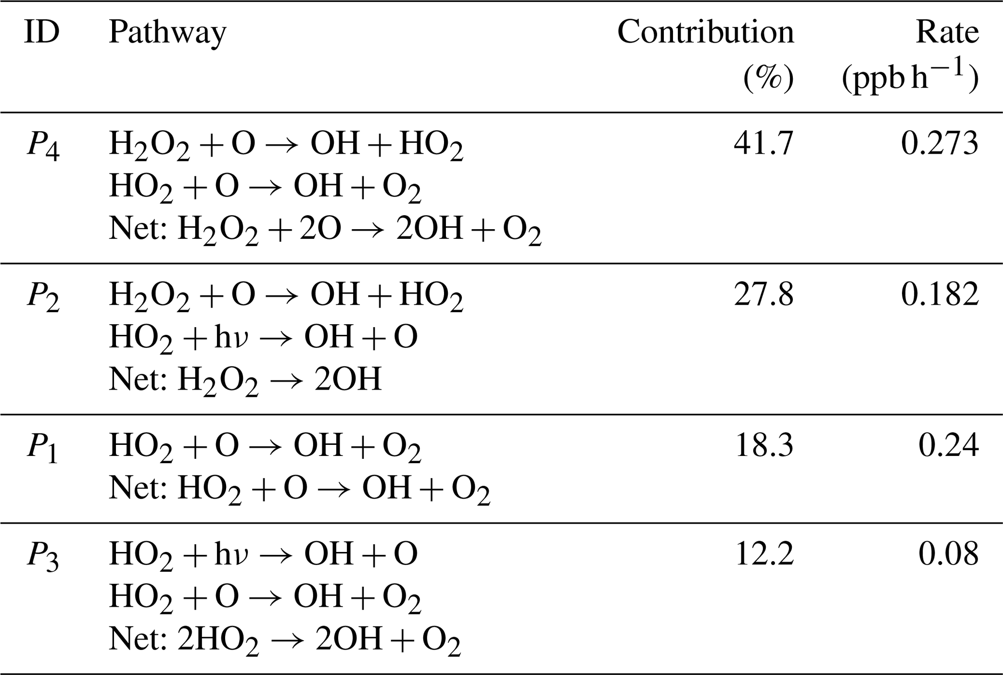
In this simple example, the pathway P₄ involving the interaction between reactions R₃ and R₅ is the most important chain of reactions for the production of OH, contributing 41.7 % of the OH production (Table 2). The interaction between reactions R₃ and R₄ (pathway P₂) is also important, contributing 27.8 % of the OH production. Deleted pathways do not contribute to the OH production, but they contribute 100 % of the OH destruction (${\stackrel{\mathrm{̃}}{C}}_d={\stackrel{\mathrm{̃}}{d}}_i/d_i=\mathrm{0.109}/\mathrm{0.109}=\mathrm{1}$). This means that if we were interested in understanding the chemical reaction chains that destroy OH in this example, we would need to repeat the analysis with a smaller f_min.

Table 2 Contribution of pathways to the production of OH in the simple example used to explain the algorithm.

In this simple example, it is easy to see that pathways P₄ and P₂ are important for OH production without using the algorithm, but when there are hundreds of reactions interacting, the pathway analysis program is a valuable tool to understand the chemical mechanisms that produce the concentration changes in a species in an atmospheric chemistry model. Also, even in this simple example, we can see how this algorithm provides valuable quantitative information about the contribution of each pathway to the production of a species.

3 Implementation

We implement the Lehmann (2004) algorithm in Python. We designed an object-oriented code script, defining a class to store the variables listed in Table 1 and separating the steps described in Sect. 2 into different class methods. We run these methods in a main method that performs the loop shown in Fig. 1. We represent the multiplicities [[x_jk]] of the pathways as a sparse matrix to optimize memory usage. Our implementation includes the option to find pathways using multiprocessing to speed up the computation time.

The code includes several functions that are useful for analyzing the pathways. After the main algorithm loop ends, the variables in Table 1 have all the information of the pathways that have been found. The code includes functions to save these variables to binary files and to read them for future analysis. The code also has functions to transform the representation of a pathway from an array of multiplicities to a string, to get the net reaction of a pathway, to create a latex table with the pathways that contribute to the production or destruction of a species of interest, and to assign a unique identifier to each pathway. This identifier is a string containing the multiplicities and the indexes of the reactions in a pathway. The same pathway can be formed multiple times during the algorithm, so we use this identifier to avoid repeating pathways. We also include a function to calculate the contribution of all pathways to the production or destruction of a species.

Our implementation includes the option to specify species that will be ignored as branching-point species. If we are interested in finding pathways at a specific timescale, it is convenient to not consider species with lifetimes longer than the timescale of interest as branching points. Our implementation also includes the option to ignore species as branching-point species by specifying a maximum lifetime of branching-point species.

3.1 Tests

The code includes run-time tests to ensure that the code works well. If the construction of pathways is correct, the rates of the reactions must be completely distributed to the pathways:

$$\begin{array}{}\text{(46)}& \left[{\mathit{r}}_j\right]=\left[{\stackrel{\mathrm{̃}}{\mathit{r}}}_j\right]+\left[\right[{\mathbf{x}}_{jk}\left]\right]\cdot [{\mathit{f}}_k{]}^T.\end{array}$$

This condition ensures that the number of molecules of a species produced or destroyed by the initial reactions is the same as the number of molecules produced or destroyed by the pathways. The code checks that Eq. (46) is fulfilled in each iteration of the algorithm and displays a warning if it is not satisfied.

The code also includes unit tests to ensure that the code works as expected in a simple scenario with four reactions representing Chapman's O₃ destruction mechanism (Chapman, 1930). This scenario was used by Lehmann (2004) to explain how the algorithm works. We include tests to ensure that our implementation finds the same pathways and rates as those found by Lehmann (2004) in this very simple example.

3.2 Tracking imbalances due to numerical errors

Before the construction of pathways, it is essential to ensure that the concentration changes in all species are balanced by the reaction's production and destruction (Eq. 1). The balance might not be fulfilled due to numerical errors. To quantify this problem, we assume that the difference between concentration changes and the total production of all reactions is due to the solver's numerical error, and we include error pseudo-reactions in the chemical system that produce or destroy a species at the rate required to fulfill the balance. We include the error pseudo-reactions in the construction of pathways. After the pathway construction finishes, we delete the pathways containing error pseudo-reactions, updating $\left[{\stackrel{\mathrm{̃}}{\mathit{r}}}_j\right]$, $[{\stackrel{\mathrm{̃}}{\mathit{p}}}_i$], and $[{\stackrel{\mathrm{̃}}{\mathit{d}}}_i$]. We also include variables similar to $[{\stackrel{\mathrm{̃}}{\mathit{r}}}_j$], $[{\stackrel{\mathrm{̃}}{\mathit{p}}}_i$], and $\left[{\stackrel{\mathrm{̃}}{\mathit{d}}}_i\right]$ to track the rates of the pathways containing error pseudo-reactions. This approach gives the user information on how important the numerical error is in explaining the concentration changes. Ideally, the pathways containing error pseudo-reactions will not contribute significantly to the concentration change that one is interested in understanding.

3.3 Using Chempath

Chempath is available at https://github.com/DanyIvan/chempath (last access: 11 July 2025). This code repository includes a tutorial on how to use Chempath, as well as some examples of how to apply Chempath to a box model and to a one-dimensional photochemical model (Sect. 4).

There are two important steps to use Chempath. First, the user needs to transform the output of a photochemical model into files readable by Chempath and balance the concentration changes if necessary (Sect. 3.2). The code repository includes some examples of how to create these input files. Second, the user needs to choose a minimum rate of pathways f_min. This can be done by trial and error or by setting it as a fraction of the rate of total production or destruction by the reactions of the species the user is interested in finding pathways for. However, this way of setting f_min might still require further trial and error to find an appropriate fraction of the total production or destruction by all reactions. Ideally, f_min will be small enough so that the deleted pathways do not contribute significantly to the production or destruction of a species of interest. However, if f_min is too small, the code might take a long time to run.

4 Application examples

Here we provide two examples of how to apply Chempath to a photochemical box model (Sect. 4.1) and to a one-dimensional photochemical model (Sect. 4.2)

4.1 Pathways in a photochemical box model

To give an example of the application of Chempath in a simple scenario, we developed a photochemical box model that solves the equation

$$\begin{array}{}\text{(47)}& {\displaystyle \frac{\mathrm{d}{\mathit{\rho }}_i}{\mathrm{d}t}}={\mathrm{\Pi }}_i-L_i,\end{array}$$

where ρ_i is the number density of a species i, Π_i is its chemical production, and L_i is its chemical destruction. We use a reaction system with 15 reactions between 8 species involving O₃ and hydrogen oxide species. All the reactions and reaction rate parameters that we use can be found at https://github.com/DanyIvan/chempath/tree/main/examples/box_model_pathways (last access: 11 July 2025). To keep the model as simple as possible, we assume that photochemical reactions have constant rate constants. We obtain these rate constants by running a more complex photochemical model that solves radiative transfer (Wogan, 2023a). We use similar rates to the ones obtained by this model at 20km in altitude. The purpose of this simple model is to provide an example of the use of the pathway analysis algorithm, not to be an accurate representation of stratospheric O₃ chemistry.

We run the box model for 80 d. All species in the model reach a steady state during this time, and there is an increase in the O₃ number density (Fig. 2a). The O₃ concentration change is the result of an imbalance between O₃ production and loss (Fig. 2d). This imbalance causes an increase in O₃ until a steady state is reached. We use Chempath to see what the most important pathways for the production and destruction of O₃ in this model run are.

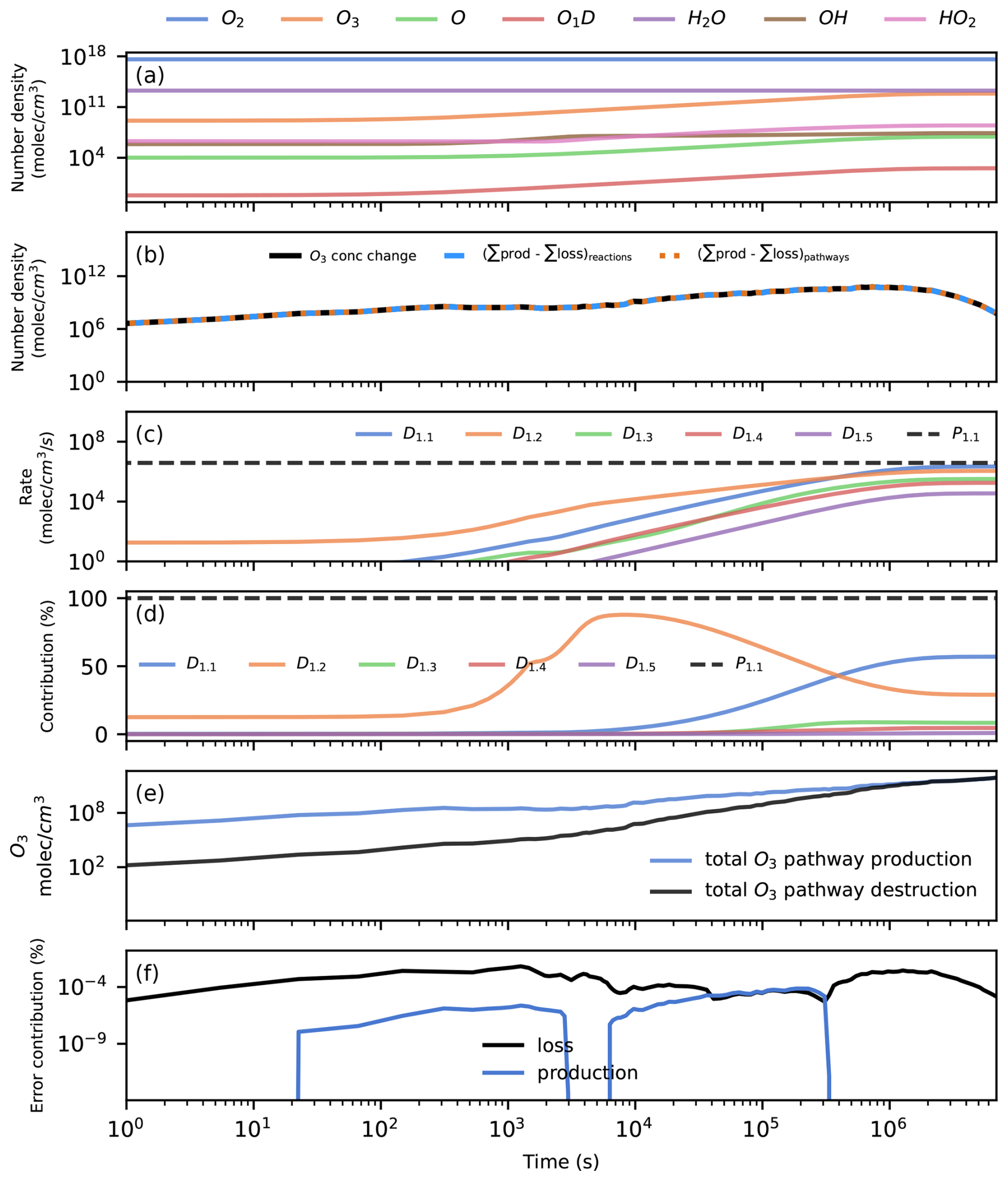
Figure 2 Application of Chempath to a simple photochemical box model. Panel (a) presents the evolution of the model over time. Panel (b) shows the O₃ concentration change over time (black line) and the total production minus the total loss from all reactions (blue dashed line) and from all pathways (orange dotted line). This panel shows that the reactions and pathways completely explain the O₃ concentration change, and Eqs. (1) and (46) are satisfied for O₃. Panels (c) and (d) show the rate and contribution of the five most important pathways for O₃ destruction (colored continuous lines) and the only pathway for O₃ production (black dotted line). These pathways can be seen in Table 3. Panel (e) shows the total O₃ production and destruction by all pathways. Panel (f) shows the contribution to O₃ production or loss from pathways containing error pseudo-reactions.

To balance the concentration changes, we include error pseudo-reactions in the reaction system that produce or destroy a species at the rate required to fulfill the balance. We calculate the rate of these error pseudo-reactions as the difference between the left- and right-hand sides of Eq. (47). After including the error pseudo-reactions, the concentration changes in all the species are explained exactly by the production and destruction caused by the reactions (Fig. 2b shows an example of this for the O₃ concentration change). The pathways containing error pseudo-reactions contribute less than 0.001 % to the O₃ concentration change across the model run (Fig. 2f).

We run Chempath to find pathways for all the model time intervals at which the solver obtained a solution for the system, setting f_min=0. The reaction rates are completely distributed to the pathways (Eq. 46 is fulfilled), so the concentration changes are explained exactly by the production and destruction caused by the pathways (Fig. 2b shows an example of this for the O₃ concentration change). There is only one O₃-producing pathway in this reaction system (pathway P₁ in Table 3 and Fig. 2c). The algorithm identified 49 O₃ destruction pathways (Fig. 2c and Table 3 present the five most important pathways). These pathways destroy O₃ through hydrogen oxide (HO_x) catalytic cycles.

Table 3 Pathways for O₃ production and destruction in the simple photochemical box model shown in Fig. 2d.

4.2 Pathways in a one-dimensional photochemical model

In this section, we show how to apply Chempath to the one-dimensional photochemical model photochem (Wogan et al., 2023, https://github.com/Nicholaswogan/photochem, last access: 11 July 2025). We run the photochem model with the “Modern Earth” reaction scheme that includes 1281 reactions between 113 species. We run the model to photochemical equilibrium using surface flux boundary conditions for O₂, CH₄, CO, and H₂. We choose fluxes of $\mathrm{3.3}\times {\mathrm{10}}^{\mathrm{11}},\mathrm{5}\times {\mathrm{10}}^{\mathrm{10}},\mathrm{1.2}\times {\mathrm{10}}^{\mathrm{8}}$, and 3×10⁹ molec. cm⁻² s⁻¹ for each of these species, respectively. The choice of these fluxes is arbitrary and was motivated by our desire to obtain similar conditions to the present atmosphere. For all other species, we use the default boundary conditions of the “Modern Earth” reaction scheme. After the model reaches equilibrium, we decrease the O₂ surface flux to 2.5×10¹¹ molec. cm⁻² s⁻¹ and run the model for 1.2 million years. The idea behind the reduction in the O₂ surface flux is to create a perturbation that causes concentration changes to explore with Chempath. The concentration of O₂ in the model is controlled mainly by the surface flux and by oxidation of reduced species like CH₄, CO, and H₂ on a timescale of millions of years (the estimated lifetime of O₂ in the modern atmosphere is ∼ 2 million years; Kasting, 2013). The photochem model uses a solver with an adaptive time step (the constrained variable order, variable-step ordinary differential equation solver (CVODE) backward differential formula (BDF) method created by Sundials Computing). In our simulation, the time step varies from 10⁻⁵ to 10¹² s.

The model output shows that O₂ and O₃ concentrations tend to decrease at all altitudes as a consequence of the decrease in the O₂ surface input flux (Fig. 3). We apply Chempath to the photochem model output to gain insight into the chemical reaction chains that produce and destroy O₃ in this model run.

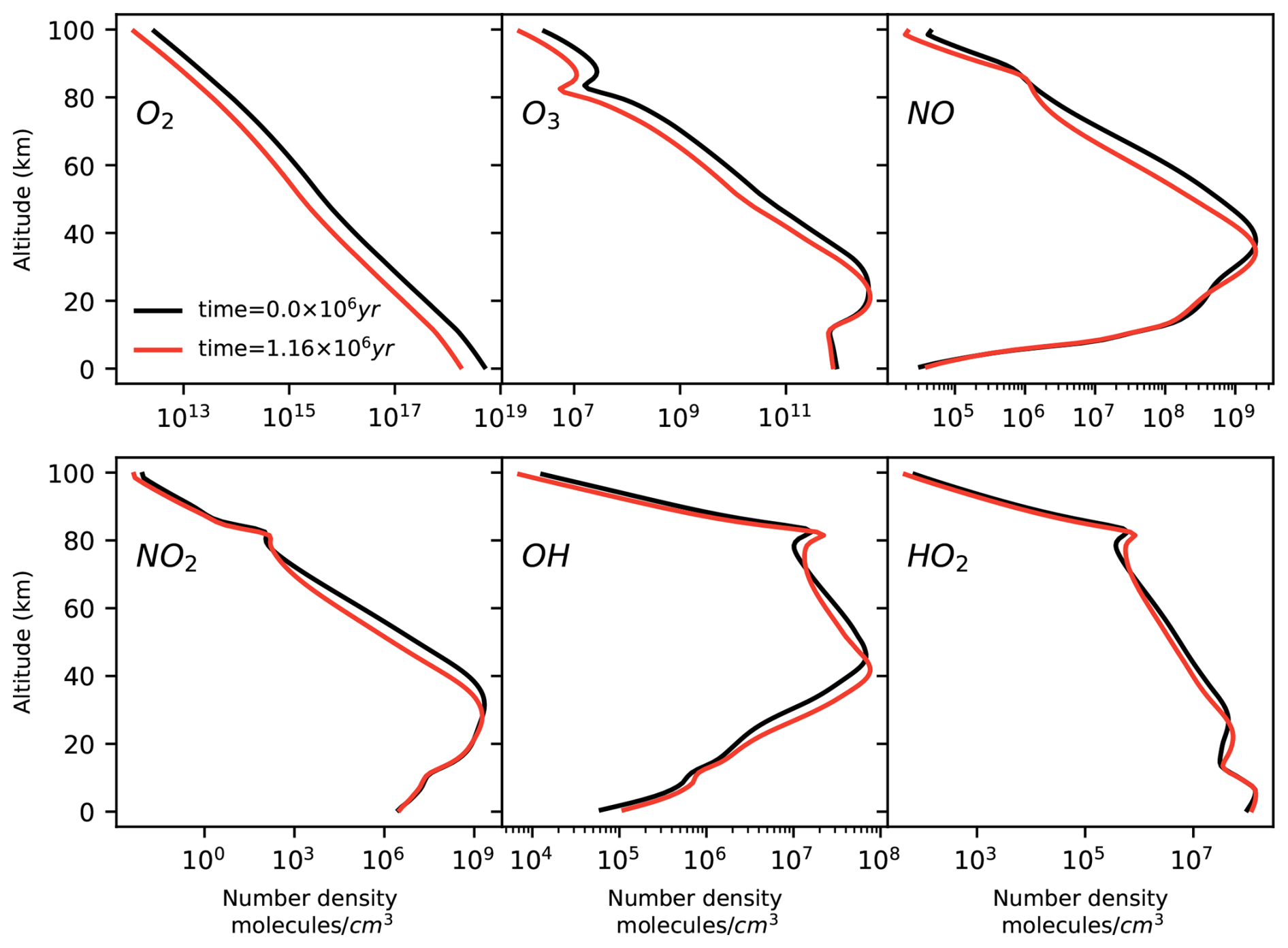
Figure 3 Number density profiles of O₂, O₃, NO, NO₂, OH, and HO₂ calculated by the photochem model at time =0.15 million years (black line) and at time =1.16 million years (red line). In this model run, we decrease the O₂ input surface flux. As a result, the O₂ and O₃ number densities tend to decrease at all altitudes. The concentrations of NO, NO₂, OH, and HO₂ decrease and increase at different altitudes.

4.3 Methods: how to find pathways in the photochem model

The application of Chempath to the photochem model output requires the inclusion of pseudo-reactions for processes that affect the concentration of species in a one-dimensional photochemical model. The photochem model calculates the concentration changes in long-lived species by solving the equation

$$\begin{array}{}\text{(48)}& {\displaystyle \frac{\partial {\mathit{\rho }}_i}{\partial t}}={\displaystyle \frac{\partial }{\partial z}}{\mathrm{\Phi }}_i+{\mathrm{\Pi }}_i-L_i-{\mathrm{\Omega }}_i+F_i,\end{array}$$

where ρ_i is the number density of species i, z is altitude, Π_i and L_i are the chemical production and destruction of species i, Φ_i is the vertical transport flux of species i, Ω_i is the destruction of species i from rainout, and F_i is a vertically distributed input flux (see Wogan et al., 2022, for more details).

We include pseudo-reactions for transport, rainout, and vertically distributed input fluxes in the reaction system at each altitude and model time in which we perform the pathway analysis:

$$\begin{array}{}\text{(49)}& \begin{array}{rl}& S_i\to S_{i{,}_{\text{trpt}}}\text{ if transport removes }{S}_i,\\ & S_{i{,}_{\text{trpt}}}\to S_i\text{ if transport supplies }{S}_i,\\ & S_i\to S_{i_{\text{ rainout}}},\\ & S_{i{,}_{\text{dist}}}\to S_i\text{ if there is a vertically distributed flux for }{S}_i.\end{array}\end{array}$$

We obtain the rate of these pseudo-reactions from the vertical transport fluxes, rainout rates, and vertically distributed fluxes calculated in the model.

To balance the concentration changes, we include error pseudo-reactions that produce or destroy a species at the rate required to achieve mass balance. We calculate the rate of these pseudo-reactions as the difference between the left- and right-hand sides of Eq. (48). The pathways containing error pseudo-reactions contribute less than 1 % of the O₃ concentration change at all times and altitudes in our analysis.

We run Chempath with the augmented reaction system at 32 time points distributed across the model run, ranging from 1 s to 1.2 million years. We find pathways at all model altitudes, except at the lower and upper boundaries. We prescribe a variable minimum pathway rate f_min that we calculate as the minimum of the chemical production from reactions (including transport pseudo-reactions) of O₂, O₃, CO, H₂, and CH₄ divided by 1000. We use these species to calculate f_min because we are interested in understanding their concentration changes. We do not consider these species to be branching points. We also ignore N₂, CO₂, and H₂O as branching-point species, treating them as long-lived inert species. Our f_min choice keeps the contribution of deleted pathways to O₃ production and destruction below 5 % at all altitudes and times in our analysis. The number of reactions with rate >f_min varies with altitude and ranges from 94 to 160.

4.4 Results: ozone destruction and production pathways in the photochem model

Chempath allows us to identify the most important pathways for O₃ production and destruction at a given altitude and time in our photochem model run (Fig. 4 and Table 4). These pathways are similar to those found in a previous study of chemical pathways affecting O₃ in the atmosphere (Grenfell et al., 2006).

In the troposphere (below 11 km in our model run), O₃ production in the photochem model is dominated by transport (pathway P_2.1) and CH₄ and CO oxidation (pathways P_2.2 and P_2.3) in the presence of nitrogen oxide radicals (NO_x). These oxidation pathways are similar to the “smog mechanism” that produces tropospheric O₃ through oxidation of hydrocarbons (Haagen-Smit, 1952; Volz-Thomas and Ridley, 1994). The tropospheric O₃ destruction is dominated by destruction by HO_x radicals (pathway D_2.1), O₃ photolysis and subsequent CH₄ oxidation (pathways D_2.2 and D_2.3), and transport (pathway D_2.4).

Table 4 Pathways producing and destroying O₃ at time=1.16 million years in the model run. The contribution profiles of these pathways are shown in Fig. 4. The contributions and rates in this table correspond to the height at which the pathways contribute the most to O₃ production and destruction. Our algorithm does not yet have the functionality to automatically order the reactions in a pathway to easily follow the flow of molecules. We ordered the reactions in all the pathways in this table by hand.

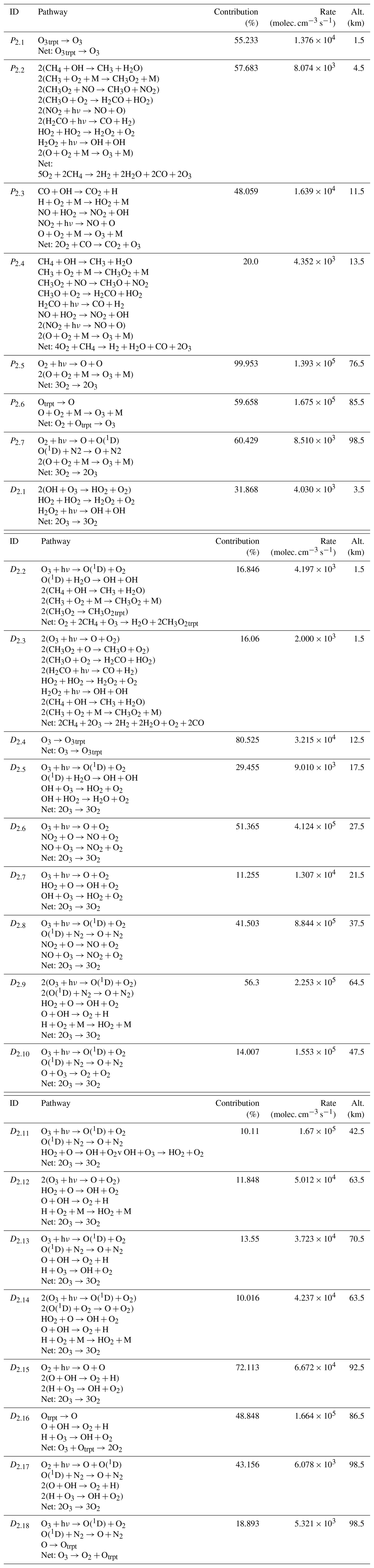
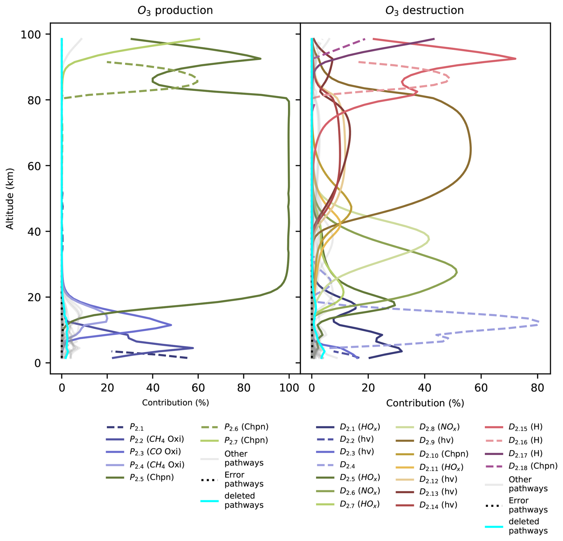
Figure 4 Contribution of pathways to O₃ production and destruction as a function of altitude at model time =1.16 million years. The main pathways are plotted in color, and the less important pathways are plotted in gray. Pathways that include transport pseudo-reactions are plotted as dashed lines. These pathways show discontinuities because transport can either supply or remove O₃ at different altitudes. The symbols in the legend group the pathways into six categories: oxidation (Oxi), Chapman-like (Chpn), photolysis (hν), hydrogen oxide (HO_x) and nitrogen oxide (NO_x) pathways, and destruction by the H atom (H). The pathways are listed in Table 4. The cyan line shows the contribution of deleted pathways, and the black dotted line shows the contribution of pathways containing error pseudo-reactions.

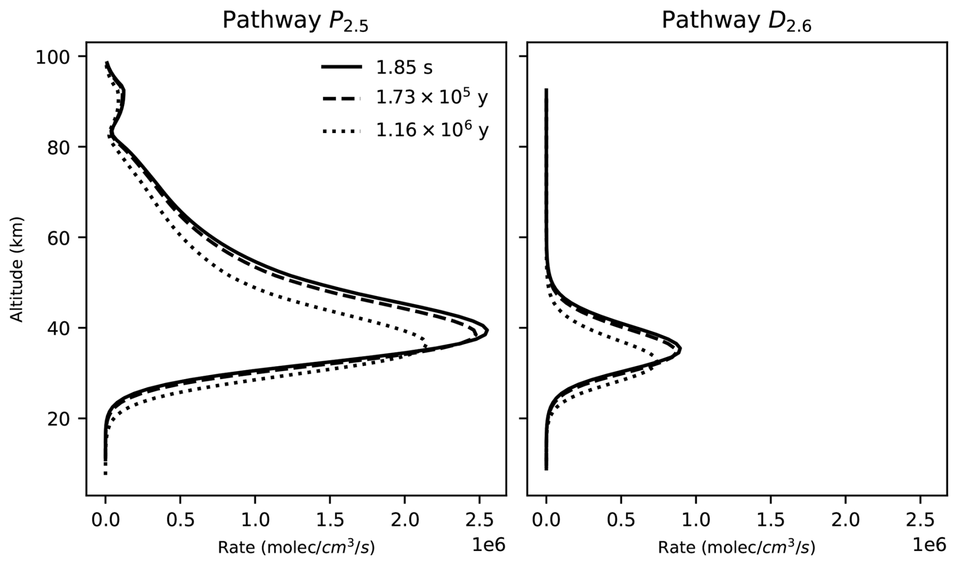
Figure 5 Rate profiles of the P_2.5 (right) and D_2.6 pathways at three different points in time across our photochem model run.

In the stratosphere (11–50 km), O₃ production mainly occurs via CO and CH₄ oxidation in the presence of NO_x radicals below 25 km (pathways P_2.3 and P_2.4) and via the Chapman production pathway P_2.5 above 25 km. The main stratospheric O₃ destruction mechanisms involve transport (pathway D_2.4), photolysis (pathway D_2.10), and destruction by HO_x radicals (pathways D_2.1, D_2.5, D_2.7, and D_2.11) and NO_x radicals (pathways D_2.6 and D_2.8). Catalytic cycles involving NO_x and HO_x radicals are important for stratospheric O₃ destruction (Lary, 1997; Jacob, 1999). Chempath can identify these well-known catalytic cycles in the photochem model.

Above 50 km in altitude, the main O₃ production mechanisms are Chapman-like production pathways (P_2.5 to P_2.7), and the main O₃ destruction mechanisms involve O₃ photolysis coupled to HO_x radical cycles, destruction by HO_x radicals, Chapman-like destruction pathways, and destruction by the H atom (D_2.9 to D_2.18).

The decrease in O₃ concentration in our model run is likely the result of a decrease in O₃ production and destruction caused by the decrease in the O₂ input flux. For example, the rate of the main stratospheric O₃-producing and O₃-destroying pathways (P_2.5 and D_2.6) decreases over time (Fig. 5). This is likely the result of the decrease in the O₂ concentration leading to a decrease in O₃ production through pathway P_2.5, causing a decrease in O₃ concentration and a subsequent decrease in the O₃ loss rate. However, the contribution profiles shown in Fig. 4 have a similar structure at all the time steps that we analyzed. Consequently, the pathways shown in Fig. 4 and listed in Table 4 are a good representation of the pathways that produce and destroy O₃ across all the times that we analyzed in our model run.

The presence of the supply by transport of the methylperoxy radical (CH₃O₂) in the pathway in D_2.2 is surprising because CH₃O₂ has a lifetime <1 min in the troposphere (Wolfe et al., 2014), and its concentration should be controlled by reactions and not by transport. This is the result of an incomplete representation of the chemistry of this species in the reaction system that we used. This reaction system is a legacy of models designed to study early-Earth and exoplanet anoxic atmospheres. Thus, the reaction system lacks some reactions for the oxidized modern-Earth atmosphere. This example illustrates how Chempath can be a great tool to understand and validate the results of photochemical models, allowing the modelers to detect potential problems with their reaction systems.

5 Conclusions

In this paper, we described the development of Chempath, an open-source pathway analysis program for photochemical models that can automatically construct the most relevant pathways of a reaction system and identify the most important pathways for the production and destruction of a species of interest. We showed how to use Chempath in a simple box model and in a one-dimensional photochemical model. Chempath identified well-known pathways for O₃ destruction and production in Earth's atmosphere, suggesting that this algorithm can be used to understand chemical mechanisms in photochemical models of less-well-known atmospheres, like those of exoplanets or past atmospheres.