SynRad v1.0: a radar forward operator to simulate synthetic weather radar observations from volcanic ash clouds

In this work, SynRad, a new radar forward operator for the Active Tracer High-Resolution Atmospheric Model (ATHAM) volcanic plume model is introduced. The operator is designed to generate synthetic radar signals from ground-based scanning weather radars for volcanic ash clouds simulated by ATHAM. A key novelty of SynRad is a ray-tracing module that traces radar beams from the antenna to the ash cloud and calculates path attenuation due to hydrometeors and ash. The operator is designed to be compatible with the one-moment microphysics scheme in ATHAM, but it can easily be extended to other one- or two-moment schemes in ATHAM or any weather prediction model. The operator can be used to test candidate locations at which to operationally deploy portable high-frequency or multi-frequency (from long to short wavelength) scanning radar(s). An optimal frequency or frequencies (for a multi-frequency radar) can be identified that balance the trade-off between a stronger return signal and the increased path attenuation that comes at these higher frequencies. A case study of the eruption of the Raikoke volcano in 2019 is used to evaluate the performance of SynRad. The measurement process of a C-band radar is simulated using SynRad, and the operator was able to generate realistic fields of the equivalent radar reflectivities, echo tops, and vertical maximum intensities. Even though higher-frequency microwave weather radars (K-band and higher) have been used to observe volcanic activity, they may not operate in scanning mode. Ideally, higher-frequency microwave radars will be designed and constructed specifically for monitoring volcanic eruptions. This is certainly possible in the coming years, making feasibility studies on the capability of higher-frequency radars timely.

1 Introduction

Active monitoring of volcanic eruptions and their subsequent ash cloud dispersal is an area of significant interest due to their human, social, and economical effects. These include direct impacts, such as the hazard to aviation via the tephra injected into the atmosphere, and primary and secondary impacts of the volcanic ash accumulating on the ground and causing damage to life and property in the surrounding areas (Jenkins et al., 2015). Real-time monitoring of the volcanic ash cloud distribution and dispersal has mainly been carried out using satellite measurements. New-generation geostationary satellites, such as Himawari-8 (Bessho et al., 2016), GOES-16, and GOES-17 (GOES-R, 2020), have a spatial resolution of about 500 m–2 km and a temporal resolution of the order of minutes. However, we do not yet have complete satellite coverage to actively monitor volcanic activity globally. Additionally, volcanic clouds are often obscured by meteorological clouds, making ground-based observations essential. Timely information and predictions of the ash cloud dispersal are vital, as most encounters with the ash cloud have historically happened within minutes to a few hours of eruptions.

Ground-based microwave scanning weather radars present a unique opportunity to monitor ash clouds with relatively higher spatial (less than a few hundred metres) and temporal (every few minutes) resolutions and for 24 h a day. These radars measure the back-scattered energy returned to the radar dish as a result of interactions between a train of short and high-powered pulses (or a continuous wave) of electromagnetic energy and the scatterers. The scatterers can be volcanic ash particles or liquid or icy meteorological particles, such as droplets, ice, or raindrops. These interactions depend on the size, shape, orientation, and distribution of the particles and the frequency and polarization of the electromagnetic radiation. The back-scattered signals measured at the radar receiving antenna are then typically converted to equivalent radar reflectivities (in decibels) – the most common and familiar quantity in meteorology (Smith, 1984).

Permanent monitoring of volcanic ash clouds using scanning weather radars operating at lower frequencies, i.e. S-, C- and X-bands, has become quite common, buoyed by the benefits of the continuous quantitative retrieval of two key source parameters that are fed into long-range ash dispersion models – the eruption plume height and the tephra eruption rate and mass. There are several ground-based scanning weather radar networks operational in Alaska, Iceland, and Italy (to name a few) that have been key in monitoring eruptions. Notable examples include the monitoring of the eruption of the Hekla volcano in 2000 (Lacasse et al., 2004) and the eruption of the Grímsvötn volcano in 2004 in Iceland (Marzano et al., 2010a) using C-band radars, monitoring of the Augustine volcanic eruption in Alaska, USA, in 2006 using S-band weather radar imagery (Marzano et al., 2010b), monitoring of the eruption of the Redoubt volcano in Alaska, USA, in 2009 (Schneider and Hoblitt, 2013) and the Eyjafjallajökull eruption in Iceland in 2010 using C-band weather radars (Marzano et al., 2011), monitoring of the Mount Etna eruption in Italy in 2011 using a mobile X-band dual-polarization radar (Marzano et al., 2013), and monitoring of the 2012 eruption of Mount Tongariro from Upper Te Maari Crater in the central North Island of Aotearoa / New Zealand using a dual-polarization radar (Crouch et al., 2014).

The ready availability of lower-frequency scanning weather radars make them convenient to monitor ash clouds (Marzano et al., 2013); however, particle size distributions and refractive indices of ash particles are quite different from those of cloud droplets, ice crystals, rain drops, graupel, or hail. The refractive index of ash is generally lower than that of water. Volcanic particles can have any size near the vent, but the ash particle sizes far away from the vent are smaller than raindrops. This means that frequencies higher than those used in weather radars have possible benefits with respect to the monitoring and measurement of volcanic ash concentrations. Additionally, successfully detecting a volcanic ash cloud using ground-based radar systems depends not only on the radar system characteristics but also on the radar range, i.e. the location at which the radar is operationally deployed with respect to the vent and the ash cloud (Marzano et al., 2013). These factors can be combined into a single parameter – the minimum detectable signal (MDS); if the return signal from a radar sample volume is higher than the MDS, the sample will be detected by the radar. Increasing the operational frequency or reducing the range can technically result in a stronger return signal from the scattering volume (Marzano et al., 2012). However, at higher frequencies (millimetre wavelengths), the two-way path attenuation plays a key role and determines the degree to which the transmitted signal can penetrate into the ash cloud. Therefore, it is important to identify plausible locations relative to the vent and the dispersing ash cloud at which to operationally deploy these millimetre-wave radars (which are often portable) that would possibly allow the radar to penetrate and scan the full extent of the ash cloud in 3D. This analysis can be done using “radar forward operators”, which are numerical operators that can generate synthetic radar signals from gridded data or 3D output from numerical simulations of volcanic eruptions.

Given certain meteorological conditions, radar forward operators have been used as a key tool to derive synthetic radar observations from numerical weather prediction (NWP) model prognostic variables. They also form a key part of inversion algorithms used to retrieve radar-observable variables or in data assimilation. These operators include numerical descriptions of the different physical aspects of radar measurements. Modelled clouds are converted to equivalent radar reflectivities in order to compare them with actual radar observations (from either ground-based radars or radars on satellites). Most operators developed so far have been polarimetric radar operators used for hydrometeor classification and improvement in weather radar data quality and rainfall measurements in addition to the validation (of microphysics modules) and assimilation of radar reflectivities into NWP models (Pfeifer et al., 2008; Cheong et al., 2008; Jung et al., 2008; Ryzhkov et al., 2011; Augros et al., 2016; Zeng et al., 2016; Hort and Scharff, 2016; Shrestha et al., 2022; Li et al., 2022; Wang et al., 2025). In this paper, we introduce SynRad, a new radar forward operator that has been exclusively designed to synthetically calculate the return signals from volcanic ash clouds and hydrometeors. Even though conventional forward operators calculate the attenuated or corrected reflectivity, they do not trace the radar beam and its extinction through the cloud under study. Some of the previously mentioned operators output the specific attenuation coefficient of each radar gate from which the path attenuation or extinction can be accumulated offline. A key aspect of SynRad is a ray-tracing module that calculates the extinction of the transmitted (and reflected) radar signal online due to interactions within the ash cloud. As previously discussed, the advent of portable millimetre-wavelength radar systems has made it important to include path attenuation in all relevant studies. A forward radar operator designed specifically for volcanic ash cloud tracking then plays a significant role in such cases, allowing for a purpose quite different from its weather counterparts by synthetically calculating the attenuated return signal at the radar.

Just as forward operators can help to improve numerical models, they also have the potential to complement the process of designing and operationally deploying portable or fixed radars. With millimetre-wave radars being considered specifically for monitoring volcanic ash clouds (Macfarlane et al., 2021), the development of such an operator and a methodology is timely to inform radar design and the overall suitability of such radars to detect volcanic ash clouds and characterize the sizes and concentrations of the volcanic ash (with multiple-frequency radars) immediately following an eruption. Key to this is identifying the optimal location and range from the volcanic vent at which it would best serve its purpose. For a known set of radar system characteristics, the synthetic radar observables can then help one decide upon optimum locations for radar deployment. They can also be used to evaluate the performance of existing fixed weather radars (with a certain MDS) for volcanic ash cloud monitoring. This will be the focus of this paper, as we introduce the workflow of SynRad and evaluate the performance of a C-band weather radar to detect the ash cloud from the 2018 eruption of the Raikoke volcano. This is also the first time the aforementioned eruption has been numerically modelled and the results presented.

In Sect. 2, the model data that serve as the input to SynRad are described. In Sect. 3, a detailed workflow of SynRad, including the theory and computational modular structure, is introduced. In Sect. 4, the main results and performance of SynRad in the C-band are evaluated using the operator on numerical simulation data of the 2019 eruption of the Raikoke volcano. Finally, in Sect. 5, the conclusions are presented along with future plans for SynRad.

2 Description of the data – input to SynRad

SynRad v1.0 generates synthetic radar signals from 3D output generated by the Active Tracer High-Resolution Atmospheric Model (ATHAM). ATHAM is a 3D, non-hydrostatic atmospheric model that has been specifically designed to simulate characteristics of volcanic eruption plumes (Oberhuber et al., 1998; Herzog et al., 2003; Herzog and Graf, 2010). ATHAM predicts the behaviour of a multicomponent system consisting of a gas–particle mixture with arbitrary tracer concentrations. Unique features of ATHAM are its dynamically and thermodynamically active tracers and its ability to represent strongly divergent flows with large vertical accelerations. The vent size, exit velocity, temperature, and composition of the mixture are prescribed as a function of time. A single-moment cloud microphysical module (Herzog et al., 1998) predicts the presence of condensed water, ice, and graupel and the effect of phase changes on the plume's heat budget, but it does not currently include interactions between hydrometeors and ash particles. Typical 3D output generated by ATHAM includes netCDF files for every minute for the wind velocities, pressure, mixture potential, and in situ temperatures and densities as well as the specific concentrations of the different ash categories, hydrometeor categories, water vapour, and gases (like SO₂).

3 SynRad methodology, workflow, and assumptions

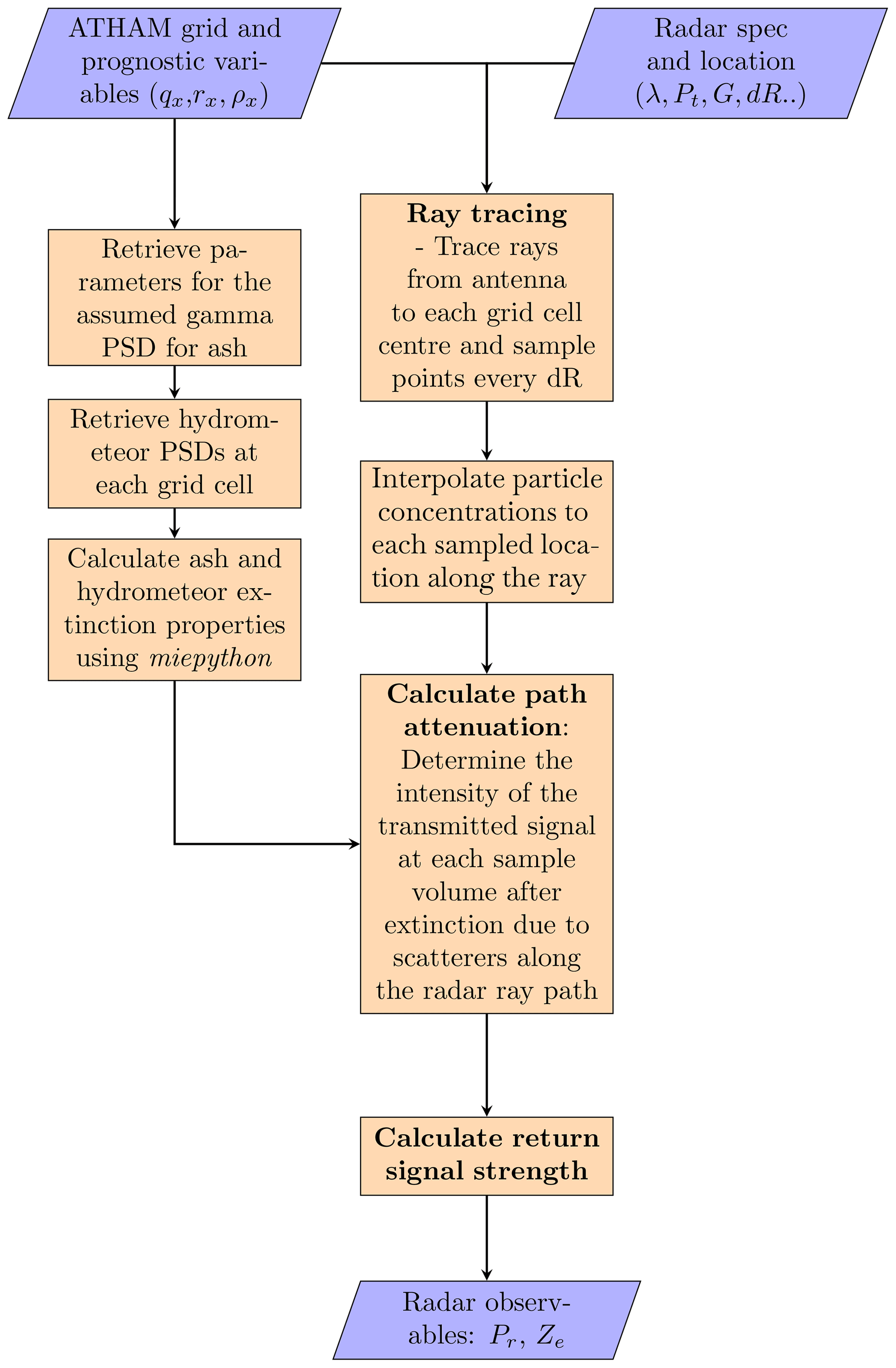
SynRad v1.0 generates synthetic radar signals by calculating the return power, path attenuation, and effective radar reflectivity (a common radar observable) from ATHAM 3D output and user-specified radar characteristics, i.e. the radar position, wavelength (or frequency), transmit power, the one-way 3 dB antenna beamwidth, and the range bin length (or resolution). For a pulsed radar, this is the pulse width, whereas for a frequency-modulated continuous-wave (FMCW) radar, this depends on the signal bandwidth. The standard workflow of SynRad is shown in Fig. 1 and detailed in the following sub-sections. For a given radar location, rays are traced from the antenna to each ATHAM grid cell centre (which acts as the radar sample volume or bin), and path attenuation is calculated at different points along this ray. In other words, a radar is placed in the numerical domain, whereas the beam paths are traced over the 3D output, cell by cell. Calculations are performed on each cell in the grid; i.e. no volume scan measurements are simulated. In this section, the methodology behind SynRad is introduced. This includes the theory behind the physical aspects of radar measurement and how this theory is implemented in SynRad via the different modules. However, we start with the assumptions made during synthetic-signal generation.

Figure 1 SynRad workflow.

3.1 Assumptions made in SynRad

In this sub-section, we list the assumptions made in the current version of SynRad. These assumptions are as follows:

1. All scattering particles (ash and hydrometeors) are homogeneous dielectric spheres that are assumed to occupy the entire resolution volume.

2. The atmosphere in which the synthetic radar beam is propagating in the model domain is assumed to be non-attenuating; i.e. we neglect attenuation due to atmospheric gases (oxygen, water vapour, and nitrogen) and only consider attenuation due to condensed water, ice crystals, and graupel, as these would dominate the attenuation field. Attenuation due to volcanic SO₂ is also neglected. The dominating attenuation in this case is due to the ash particles and hydrometeors; hence, the decision was made to neglect attenuation due to gases.

3. Beam bending due to atmospheric refraction along its trajectory is neglected.

4. The effects of multiple scattering within a resolution volume is ignored.

5. A single-polarization radar is considered where the incident and back-scattered waves are linearly polarized. A polarimetric radar sends out signals that are oriented vertically and horizontally; thus, by comparing the reflected signals from both orientations, different precipitation types can be identified. Here, we only consider horizontally polarized signals. Thus, the effect of polarization is not considered, but this is something that will be added in upcoming versions. This would also include considering non-sphericity and orientation preferences for the ash and hydrometeors.

3.2 Radar measurement theory

For a radar with transmitted power P_t (W), antenna gain G, one-way normalized radiation pattern $\left|f\right({\mathit{\theta }}_{\mathrm{1}},{\mathit{\varphi }}_{\mathrm{1}}){|}^{\mathrm{2}}$ (where (θ,ϕ) defines the half-power beam width (for one-way transmission)), and effective antenna aperture A_e, the power received by the antenna from all volume-distributed targets in a radar resolution volume dV that is spanned by a solid angle dΩ and range resolution dR is given by the following (Probert-Jones, 1962):

$$\begin{array}{}\text{(1)}& \text{d}{P}_{\mathrm{r}}={\displaystyle \frac{P_{\mathrm{t}}\mathrm{d}\mathrm{\Omega }}{\left(\mathrm{4}\mathit{\pi }\right)}}G\left|f\right(\mathit{\theta },\mathit{\varphi }){|}^{\mathrm{2}}\mathrm{d}R\cdot A_{\mathrm{e}}|f(\mathit{\theta },\mathit{\varphi }){|}^{\mathrm{2}}{\displaystyle \frac{\mathrm{1}}{\mathrm{4}\mathit{\pi }{R}^{\mathrm{2}}}}\cdot \mathit{\eta }\cdot \mathrm{d}\mathrm{\Omega },\end{array}$$

where η is the volumetric radar reflectivity (m⁻¹) and dΩ is subtended by an area da (m²) at a range R (m). We can relate A_e to the antenna gain by $A_{\mathrm{e}}=\frac{{\mathit{\lambda }}^{\mathrm{2}}}{\mathrm{4}\mathit{\pi }}G$, where λ is the radar wavelength (m). The total power received at the same instance of time is then obtained by integrating in range over the resolution δ and over the solid angle Ω subtended by that portion of the surface of the sphere (of radius R) giving the following:

$$\begin{array}{}\text{(2)}& P_{\mathrm{r}}=\underset{R}{\overset{R+\mathit{\delta }}{\int }}\underset{\mathrm{\Omega }}{\int }\mathrm{d}{P}_{\mathrm{r}}={\displaystyle \frac{P_{\mathrm{t}}{\mathit{\lambda }}^{\mathrm{2}}{G}^{\mathrm{2}}}{(\mathrm{4}\mathit{\pi }{)}^{\mathrm{3}}}}\underset{R}{\overset{R+\mathit{\delta }}{\int }}{\displaystyle \frac{\mathrm{d}R}{R^{\mathrm{2}}}}\cdot \underset{\mathrm{d}\mathrm{\Omega }}{\int }\left|f\right(\mathit{\theta },\mathit{\varphi }){|}^{\mathrm{4}}\cdot \mathit{\eta }.\end{array}$$

As R≫δ, the first integral gives

$$\begin{array}{}\text{(3)}& \underset{R}{\overset{R+\mathit{\delta }}{\int }}{\displaystyle \frac{\mathrm{d}R}{R^{\mathrm{2}}}}={\displaystyle \frac{\mathit{\delta }}{R^{\mathrm{2}}}},\end{array}$$

and the second integral can be evaluated to (Probert-Jones, 1962)

$$\begin{array}{}\text{(4)}& \underset{\mathrm{d}\mathrm{\Omega }}{\int }\left|f\right(\mathit{\theta },\mathit{\varphi }){|}^{\mathrm{4}}={\displaystyle \frac{\mathit{\pi }{\mathit{\varphi }}_{\mathrm{1}}{\mathit{\theta }}_{\mathrm{1}}}{\mathrm{8}\ln \mathrm{2}}}.\end{array}$$

For an FMCW radar, the range resolution $\mathit{\delta }=c/\mathrm{2}B$, where c is the speed of light and B is the chirp bandwidth. This finally yields

$$\begin{array}{}\text{(5)}& P_{\mathrm{r}}=P_{\mathrm{0}}{\displaystyle \frac{{\mathit{\lambda }}^{\mathrm{2}}{G}^{\mathrm{2}}}{(\mathrm{4}\mathit{\pi }{)}^{\mathrm{3}}}}{\displaystyle \frac{c}{\mathrm{2}B{R}^{\mathrm{2}}}}\cdot {\displaystyle \frac{\mathit{\pi }{\mathit{\varphi }}_{\mathrm{1}}{\mathit{\theta }}_{\mathrm{1}}}{\mathrm{8}\ln \mathrm{2}}}\cdot \mathit{\eta }.\end{array}$$

This is the form of the radar range equation that forms the basis of SynRad. Equation (5) is valid for a non-attenuating medium. For an attenuating medium, the radar equation is

$$\begin{array}{}\text{(6)}& P_{\mathrm{r}}=P_{\mathrm{0}}{\displaystyle \frac{{\mathit{\lambda }}^{\mathrm{2}}{G}^{\mathrm{2}}}{(\mathrm{4}\mathit{\pi }{)}^{\mathrm{3}}}}{\displaystyle \frac{c}{\mathrm{2}B{R}^{\mathrm{2}}}}\cdot {\displaystyle \frac{\mathit{\pi }{\mathit{\varphi }}_{\mathrm{1}}{\mathit{\theta }}_{\mathrm{1}}}{\mathrm{8}\ln \mathrm{2}}}\cdot \mathit{\eta }\cdot L^{\mathrm{2}},\end{array}$$

where L is the one-way path attenuation factor from the radar antenna to the considered range bin. The squaring (L² term) implies two-way path attenuation and quantifies the damping of the radar signal as it propagates through the atmosphere to the volcanic ash plume and back to the radar antenna. Equation (6) can be simplified to the working form used in SynRad:

$$\begin{array}{}\text{(7)}& P_{\mathrm{r}}=C_{\mathrm{r}}{\displaystyle \frac{Z}{R^{\mathrm{2}}}}{L}^{\mathrm{2}},\end{array}$$

where $C_{\mathrm{r}}=\frac{P_{\mathrm{0}}{G}^{\mathrm{2}}}{\mathrm{64}}\frac{{\mathit{\pi }}^{\mathrm{3}}}{{\mathit{\lambda }}^{\mathrm{2}}}\frac{c}{\mathrm{2}B}\frac{{\mathit{\varphi }}_{\mathrm{1}}{\mathit{\theta }}_{\mathrm{1}}}{\mathrm{8}\ln \mathrm{2}}\left|K^{\mathrm{2}}\right|$ is the radar constant that is specific to the radar system and Z is the radar reflectivity factor (m⁶ m⁻³) (Marzano and Ferrauto, 2003). The relation between η and Z is introduced in Sect. 3.3.2.

3.3 Synthetic radar signal simulation

The synthetic radar signal simulation model involves two modules: (1) the ray-tracing module, which simulates the propagation and extinction of the radar beam by hydrometeors and volcanic ash, and (2) the radar reflectivity module, which takes in the specific concentrations (and number concentrations for a two-moment microphysics scheme) of the scatterers and calculates the radar reflectivities.

3.3.1 Ray-tracing and path attenuation calculation

This module measures the extinction of the radar signal due to ash or hydrometeors along its path. The exponential decay of the amplitude of a radar signal P propagating a radial distance r in an attenuating medium can be calculated as follows:

$$\begin{array}{}\text{(8)}& P=P_{\mathrm{0}}{e}^{-\mathrm{2}{\int }_{\mathrm{0}}^r\mathit{\kappa }\left(r\right)\mathrm{d}r},\end{array}$$

where κ (m⁻¹) is the volumetric specific attenuation or extinction coefficient given by

$$\begin{array}{}\text{(9)}& \mathit{\kappa }=\underset{D_{\mathrm{1}}}{\overset{D_{\mathrm{2}}}{\int }}{\mathit{\sigma }}_e(D,f,\mathit{ϵ})N\left(D\right)\mathrm{d}D.\end{array}$$

Here, ${\mathit{\sigma }}_e={\mathit{\sigma }}_{\mathrm{s}}+{\mathit{\sigma }}_{\mathrm{a}}$ is the extinction cross-section (m²), and σ_s and σ_a are the respective scattering and absorption cross-sections (m²) for a particle of a given diameter D at a frequency f and permittivity ϵ. The exponential on the right-hand side of Eq. (8) is the two-way path attenuation factor L² (Marzano et al., 2003), i.e.

$$\begin{array}{}\text{(10)}& L^{\mathrm{2}}\left(r\right)=e^{-\mathrm{2}{\int }_{\mathrm{0}}^r\mathit{\kappa }\left(r\right)\mathrm{d}r}.\end{array}$$

With the radar location as the starting point, a ray is traced to the centre of each cell in the 3D grid of the host-model output. Each ray is then divided into n segments, and the values of the ash- and hydrometeor-specific concentrations are linearly interpolated to the end points of each segment. Starting with an initial transmitted power P₀ at the radar, the transmittance $P/P_{\mathrm{0}}$ is calculated at each segment centre using Eq. (8). The final value of P at the cell centre of the segment that acts as the end of the ray is calculated as a cumulative product of the transmittance at each ray segment. In this manner, rays are traced to every cell of the 3D grid with total scattering-specific concentrations above a threshold. Each cell corresponds to a radar resolution volume, which is associated with a particular value of P_r and Z according to Eq. (7). For a given set of radar system characteristics with a minimum detectable signal (MDS), we then discard all the rays where the return signal strength P_r is below the MDS. Every microwave radar system is assigned an MDS that assumes the noise figure of the radar receiver and is generally an available characteristic that assumes different values for a specific radar system. Alternately, the MDS can be calculated from Eq. (7) using a known minimum equivalent radar reflectivity Z_e (dBZ) for a specific radar system.

3.3.2 Radar reflectivity module

The radar reflectivity module takes in the host-model prognostic variables, such as specific concentration q (kg kg⁻¹) (for one-moment microphysics schemes) and total number concentration N_T (m⁻³) (for two-moment schemes), and returns the equivalent radar reflectivity Z_e (dBZ). Z_e is the radar-observed reflectivity and includes contributions from both ash (Z_e,ash) and hydrometeors, the latter of which include (for ATHAM) cloud droplets (Z_e,cld), pure rainwater (Z_e,rn), ice crystals (Z_e,ice), and graupel (Z_e,graup). A separate gamma function is used to describe the size distribution of ash and hydrometeors. Conventional single-polarization Doppler precipitation radars measure the horizontally polarized volumetric radar reflectivity (η in Eq. 6), which is the summation over all back-scattering cross-sections in a resolution volume at a particular bin range, as follows:

$$\begin{array}{}\text{(11)}& {\mathit{\eta }}_H=\underset{D_{\mathrm{1}}}{\overset{D_{\mathrm{2}}}{\int }}{\mathit{\sigma }}_{\mathrm{b}}(D,f,\mathit{ϵ})N(D,f,\mathit{ϵ})\text{d}D,\end{array}$$

where σ_b (m²) is the back-scattering cross-sectional area, N(D) is the number of scattering particles of diameter D per radar sample volume (m⁻⁴), and D₁ and D₂ are the respective minimum and maximum particle diameters in the sample volume (Sauvageot, 1992; Bringi and Chandrasekar, 2001). As we only consider single-polarization radars in this study, the subscript “H” will be dropped for the rest of the paper.

The module calculates the back-scattering cross-section and, thereafter, the radar reflectivity based on both the Rayleigh approximation and Mie theory. The Rayleigh scattering approximation is valid for a spherical particle with diameter D≪λ (or $\frac{\mathrm{2}\mathit{\pi }D}{\mathit{\lambda }}\ll \mathrm{1}$), in which case σ_b can be approximated as follows:

$$\begin{array}{}\text{(12)}& {\mathit{\sigma }}_{\mathrm{b}}\left(D\right)={\displaystyle \frac{{\mathit{\pi }}^{\mathrm{5}}|K{|}^{\mathrm{2}}}{{\mathit{\lambda }}^{\mathrm{4}}}}{D}^{\mathrm{6}},\end{array}$$

where $|K{|}^{\mathrm{2}}$ is the complex dielectric factor of the scatterer.

Combining Eqs. (11) and (12), under the Rayleigh approximation, gives

$$\begin{array}{}\text{(13)}& \mathit{\eta }={\displaystyle \frac{{\mathit{\pi }}^{\mathrm{5}}|K{|}^{\mathrm{2}}}{{\mathit{\lambda }}^{\mathrm{4}}}}\underset{D_{\mathrm{1}}}{\overset{D_{\mathrm{2}}}{\int }}{D}^{\mathrm{6}}N\left(D\right)\mathrm{d}D.\end{array}$$

The estimate of the radar reflectivity factor from the droplet size distributions can be expressed as the sixth moment of the drop size distribution (DSD):

$$\begin{array}{}\text{(14)}& Z=\underset{\mathrm{0}}{\overset{\mathrm{\infty }}{\int }}N\left(D\right)D^{\mathrm{6}}\mathrm{d}D,\end{array}$$

for which an analytical solution exists if we are assuming a gamma distribution for the scatterer sizes (details in Sect. 3.3.3). This gives the following (Sauvageot, 1992; Bringi and Chandrasekar, 2001):

$$\begin{array}{}\text{(15)}& \mathit{\eta }={\displaystyle \frac{{\mathit{\pi }}^{\mathrm{5}}|K{|}^{\mathrm{2}}}{{\mathit{\lambda }}^{\mathrm{4}}}}Z.\end{array}$$

As the Rayleigh approximation does not always hold and the scatterers could be categories other than liquid water (e.g. ice, ash, and graupel), the default is to calculate η using the Mie solutions and relate this to an “effective” or “equivalent” reflectivity factor Z_e which is defined as

$$\begin{array}{}\text{(16)}& Z_{\mathrm{e}}={\displaystyle \frac{{\mathit{\lambda }}^{\mathrm{4}}}{{\mathit{\pi }}^{\mathrm{5}}|K_{\mathrm{w}}{|}^{\mathrm{2}}}}\mathit{\eta }.\end{array}$$

Here, $|K_{\mathrm{w}}{|}^{\mathrm{2}}$ is the dielectric factor for water, which is to account for the fact that scatterers are expected to be spherical water droplets. Hence, for water droplets in the Rayleigh regime, Z_e=Z. The equivalent reflectivity factor Z_e is, therefore, the radar reflectivity of a target consisting of water drops (with D≪λ) which would produce the same reflectivity as that of a target with known properties (American Meteorological Society, 2012).

The Mie solutions for the back-scattering cross-section of N dielectric homogeneous spherical particles are given by the following (Mie, 1908):

$$\begin{array}{}\text{(17)}& {\mathit{\sigma }}_{\mathrm{b}}={\displaystyle \frac{{\mathit{\lambda }}^{\mathrm{2}}}{\mathrm{2}\mathit{\pi }}}\sum _{n=\mathrm{1}}^N(\mathrm{2}n+\mathrm{1})|a_n{|}^{\mathrm{2}}+|b_n{|}^{\mathrm{2}},\end{array}$$

where the Mie coefficients a_n and b_n are spherical Bessel functions depending on the refractive index m and a size parameter $x=\mathit{\pi }D/\mathit{\lambda }$. These solutions provide the more accurate description but can be computationally intensive. In this module, the “miepython” Python package is used to efficiently calculate the back-scattering cross-sections according to Mie theory and following the procedure described by Wiscombe (1979). The miepython package takes the size parameter x and the refractive index m of the scatterer as input. Therefore, while using the Mie formulas, Z_e is calculated using Eq. (16), with η calculated using Eq. (11) as a function of the frequency f and the refractive index m of the hydrometeor under consideration, and σ_b is calculated using miepython. Section 3.4 details the calculation of the complex permittivity and the refractive indices for the scatterers to be used in miepython.

It is worth mentioning that the equivalent reflectivity factor Z_e and the received power P_r are also expressed in logarithmic powers dBZ_e and dBm, respectively, as their values can vary over orders of magnitude. These are expressed as ${\text{dBZ}}_e={\text{log}}_{\mathrm{10}}(Z_{\mathrm{e}}/Z_{\mathrm{0}})$ and $\text{dBm}={\text{log}}_{\mathrm{10}}(P_{\mathrm{r}}/P_{\mathrm{r}\mathrm{0}})$, respectively, where Z₀=1 mm⁶ m⁻³ is a reference value calculated for a droplet/particle of size 1 mm and P_r0 is a reference power of  1m W. Another point to note is that, as Z_e is calculated in standard units of m⁶ m⁻³, Z₀ has to be converted to the same units by multiplying by a factor of 10⁻¹⁸.

3.3.3 Particle size distribution

In this sub-section, the different forms of the particle size distributions (PSDs) used to describe the particles existing per unit resolution volume and unit size are introduced. The code can work with both a monodisperse and a polydisperse distribution of particles. Furthermore, a gamma function is usually used to describe a polydisperse PSD of ash or hydrometeors. A general form of the gamma distribution function used to describe the polydisperse PSD of any particle category is given by the following:

$$\begin{array}{}\text{(18)}& N\left(D_x\right)=N_{\mathrm{T}x}{\displaystyle \frac{{\mathit{\alpha }}_x}{\mathrm{\Gamma }\left({\mathit{\nu }}_x\right)}}{\mathit{\lambda }}_x^{{\mathit{\alpha }}_x{\mathit{\nu }}_x}{D}_x^{{\mathit{\alpha }}_x{\mathit{\nu }}_x-\mathrm{1}}{e}^{-({\mathit{\lambda }}_x{D}_x{)}^{{\mathit{\alpha }}_x}},\end{array}$$

where N(D_x) is the total number concentration per unit volume of ash or hydrometeor of category x of diameter D_x (m⁻⁴), N_Tx is the total number concentration of the same category (m⁻³), λ_x is the slope parameter (m⁻¹), ν_x and α_x are the dispersion functions (dimensionless), and Γ is the gamma function. This generalized gamma function can be simplified further by setting α_x=1 to give the gamma function that is a three-parameter function involving N_0x, λ_x, and ν_x and is expressed as follows:

$$\begin{array}{}\text{(19)}& N\left(D_x\right)=N_{\mathrm{0}x}{D}_x^{{\mathit{\nu }}_x-\mathrm{1}}{e}^{-\left({\mathit{\lambda }}_x{D}_x\right)},\end{array}$$

where N_0x is the total number concentration parameter (${\mathrm{m}}^{-({\mathit{\nu }}_{\mathrm{x}}+\mathrm{3})}$ ) given by

$$\begin{array}{}\text{(20)}& N_{\mathrm{0}x}={\displaystyle \frac{N_{\mathrm{T}x}}{\mathrm{\Gamma }\left({\mathit{\nu }}_x\right)}}{\mathit{\lambda }}_x^{{\mathit{\nu }}_x}.\end{array}$$

For a value of ν=1, the gamma distribution reduces to the inverse-exponential or Marshall–Palmer distribution (Marshall and Palmer, 1948), in which case N_0x (with dimensions m⁻⁴) is commonly referred to as the intercept parameter. The different categories are x= {ash, cloud droplet, raindrop, ice crystal, graupel}. In addition to having different sizes and phase, raindrops and graupel are considered to be sedimenting, and graupel has a higher density than ice.

Most atmospheric models employ a moment-based microphysics scheme for the treatment of cloud microphysics. The main essence of these schemes involves assuming that the PSD can be pre-described using a functional form such as the gamma distribution function and that one or more of the moments of the PSD are simulated prognostically. An analytical solution for M_p, the pth moment of the size distribution, can be expressed as follows:

$$\begin{array}{}\text{(21)}& M_x\left(p\right)=\underset{\mathrm{0}}{\overset{\mathrm{\infty }}{\int }}{D}_x^{p}N\left(D_x\right)\mathrm{d}{D}_x={\displaystyle \frac{N_{\mathrm{T}x}}{{\mathit{\lambda }}_x^p}}{\displaystyle \frac{\mathrm{\Gamma }({\mathit{\nu }}_x+p)}{\mathrm{\Gamma }\left({\mathit{\nu }}_x\right)}}.\end{array}$$

One-moment schemes (such as that used in ATHAM to describe the microphysics) predict the specific concentration q_x (M(3)) of the different categories after specifying N_0x and ν_x. Then, with the definition of M_x given by Eq. (21), λ_x can be related to N_Tx and q_x. The mass m_x of a hydrometeor species is related to its diameter D_x through $m_x=c_{m_x}{D}_x^{p_{m_x}}$, where $c_{m_x}$ and $p_{m_x}$ are constants. For simplicity, we assume a spherical shape for all ash and hydrometeors in this work; this means that $c_{m_x}=\frac{\mathit{\pi }}{\mathrm{6}}{\mathit{\rho }}_x$, where ρ_x is the particle density and $p_{m_x}=\mathrm{3}$. The specific concentration q_x is given by

$$\begin{array}{}\text{(22)}& \begin{array}{rl}{q}_x& =\underset{\mathrm{0}}{\overset{\mathrm{\infty }}{\int }}{\displaystyle \frac{{\mathit{\rho }}_x}{\mathit{\rho }}}{\displaystyle \frac{\mathit{\pi }}{\mathrm{6}}}{D}_x^{\mathrm{3}}N\left(D_x\right)\mathrm{d}{D}_x,\\ & ={\displaystyle \frac{\mathit{\pi }}{\mathrm{6}}}{\displaystyle \frac{{\mathit{\rho }}_x}{\mathit{\rho }}}{\displaystyle \frac{N_{\mathrm{0}x}}{{\mathit{\lambda }}_x^{{\mathit{\nu }}_x+\mathrm{3}}}}\mathrm{\Gamma }({\mathit{\nu }}_x+\mathrm{3}).\end{array}\end{array}$$

The slope parameter λ_x can then be derived as follows:

$$\begin{array}{}\text{(23)}& {\mathit{\lambda }}_x={\left({\displaystyle \frac{\mathit{\pi }}{\mathrm{6}}}{\displaystyle \frac{{\mathit{\rho }}_x}{\mathit{\rho }}}{\displaystyle \frac{N_{\mathrm{0}x}}{q_x}}\mathrm{\Gamma }({\mathit{\nu }}_x+\mathrm{3})\right)}^{\mathrm{1}/({\mathit{\nu }}_x+\mathrm{3})}.\end{array}$$

The radar reflectivity module in SynRad starts with calculating N_0x or λ_x from q_x using Eq. (23). For the hydrometeors, a size distribution N_Dx to be used in Eq. (11) is then generated from Eq. (19) using known constant values of N_0x and ν_x. For the ash particles, N0_ash is calculated by rearranging Eq. (22) and using values of λ_ash and ν_ash retrieved from the initial size distribution and described in Sect. 4.1.1.

3.4 Calculation of complex permittivity

At microwave frequencies, the dielectric properties of air, water, and ice can be expressed using the complex permittivity $\mathit{ϵ}={\mathit{ϵ}}^{\prime }+i{\mathit{ϵ}}^{\prime \prime }$, where the first term is the real part of the permittivity and the imaginary part ϵ^′′ is the loss factor. The complex refractive index can also be represented in a similar form: $m=m^{\prime }+i{m}^{\prime \prime }$. The relation $m=\sqrt{\mathit{ϵ}}$ is used to relate the two quantities.

The dielectric constant of water is usually modelled using the Debye formula (Liebe et al., 1991), which is given by the following

$$\begin{array}{}\text{(24)}& {\displaystyle }{\mathit{ϵ}}_{\mathrm{w}}^{\prime }={\mathit{ϵ}}_{\mathrm{\infty }}+[{\mathit{ϵ}}_{\mathrm{s}}-{\mathit{ϵ}}_{\mathrm{\infty }}]/[\mathrm{1}+({\mathit{\lambda }}_{\mathrm{s}}/\mathit{\lambda }{)}^{\mathrm{2}}],\text{(25)}& {\displaystyle }{\mathit{ϵ}}_{\mathrm{w}}^{\prime \prime }=[{\mathit{ϵ}}_{\mathrm{s}}-{\mathit{ϵ}}_{\mathrm{\infty }}({\mathit{\lambda }}_{\mathrm{s}}/\mathit{\lambda }\left)\right]/[\mathrm{1}+({\mathit{\lambda }}_{\mathrm{s}}/\mathit{\lambda }{)}^{\mathrm{2}}],\end{array}$$

where ϵ_∞ is the high-frequency dielectric constant (f→∞), ϵ_s is the static constant, and λ_s is the relaxation wavelength (Ray, 1972).

The model proposed in Hufford (1991) is used to calculate the dielectric constant of ice:

$${\mathit{ϵ}}_{\mathrm{i}}^{\prime }=\mathrm{3.15},{\mathit{ϵ}}_{\mathrm{i}}^{\prime \prime }=\mathit{\alpha }\left(T\right)/f+\mathit{\beta }\left(T\right)f,$$

where T is the temperature (in °C). The coefficients α (GHz⁻¹) and β (GHz⁻¹) are given by the following:

$$\begin{array}{c}{\displaystyle }\mathit{\alpha }=(\mathrm{50.4}+\mathrm{62}\mathit{\theta })\times {\mathrm{10}}^{-\mathrm{4}}{e}^{-\mathrm{22.1}\mathit{\theta }};\\ {\displaystyle }\begin{array}{rl}& \mathit{\beta }=\left({\displaystyle \frac{\mathrm{0.502}-\mathrm{0.131}\mathit{\theta }}{\mathrm{1}+\mathit{\theta }}}\right)\times {\mathrm{10}}^{-\mathrm{4}}+\mathrm{0.542}\\ & \times {\mathrm{10}}^{-\mathrm{6}}{\left({\displaystyle \frac{\mathrm{1}+\mathit{\theta }}{\mathit{\theta }+\mathrm{0.0073}}}\right)}^{\mathrm{2}},\text{with}\end{array}\\ {\displaystyle }\mathit{\theta }={\displaystyle \frac{\mathrm{300}}{\mathrm{273.15}+T}}-\mathrm{1}.\end{array}$$

The complex dielectric constant of graupel is calculated by considering graupel as a mixture of ice and air (Ryzhkov et al., 2011). The final form of the equation can be represented in the Debye form as follows:

$$\begin{array}{}\text{(26)}& {\displaystyle \frac{{\mathit{ϵ}}_{\mathrm{g}}-\mathrm{1}}{{\mathit{ϵ}}_{\mathrm{g}}+\mathrm{2}}}={\displaystyle \frac{{\mathit{\rho }}_{\mathrm{g}}}{{\mathit{\rho }}_{\mathrm{i}}}}{\displaystyle \frac{{\mathit{ϵ}}_{\mathrm{i}}-\mathrm{1}}{{\mathit{ϵ}}_{\mathrm{i}}+\mathrm{2}}},\end{array}$$

where ρ_g=700 and ρ_i=917 are the densities of graupel and ice, respectively.

The complex refractive index of ash is taken as $m_{\mathrm{ash}}=\mathrm{2.5}-\mathrm{0.03}j$ (Marzano et al., 2006).

4 Application

4.1 Case study - the 2019 Raikoke eruption

The eruption of the Raikoke volcano on 21 June 2019 is selected to demonstrate the working of SynRad v1.0. Raikoke is located at 48.2° N, 153.3°E and is on an uninhabited, small (4.6 km²) volcanic island situated near the middle of the Kuril Islands archipelago in the Sea of Okhotsk in the northwest Pacific Ocean. No monitoring stations with microwave weather radars tracked the eruption, and existing studies have all employed satellite data. The eruption lasted 3.5 h, and the ash cloud rose to a height of 13 km a.s.l. Due to the lack of field studies, the ash size distribution from the 2011 Grímsvötn eruption is adopted to numerically model the Raikoke eruption using ATHAM. The initial sizes and specific concentrations of the initial ash distribution are given in Table 2. For the purpose of evaluating SynRad, we place a C-band weather radar approximately 17 km south of the vent in the numerical domain. The radar has the same characteristics as the EEC MM-250C Doppler meteorological radar used in Schneider and Hoblitt (2013) to monitor the Redoubt eruption in Alaska. The characteristics required as input to SynRad are given in Table 1. The MDS is calculated for this radar system using a minimum detectable dBZ of 0 dBZ.

Table 1 Specifications of the weather radar for which synthetic signals are generated using SynRad.

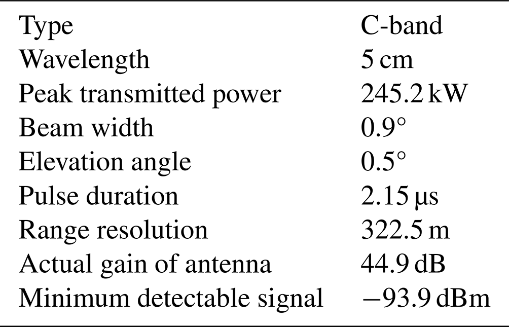
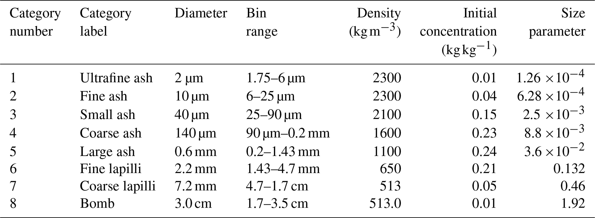
Table 2 Properties of the initial grain size distribution for the Raikoke eruption modelled using ATHAM. The size parameter $x=\mathit{\pi }D/\mathit{\lambda }$.

4.1.1 Retrieving the parameters of the ash size distribution

Assuming a gamma distribution, the initial ash sizes are binned into eight different ash categories with different radii and densities, as given in Table 2. It should be noted that specific concentrations are cited in units of kilograms per kilogram (kg kg⁻¹) in Table 2, as this is the standard unit for the specific concentration prognostic variable in ATHAM (mass per unit kilogram of total mixture). For the rest of the paper, the concentrations are cited in grams per cubic metre (g m⁻³) or kilograms per cubic metre (kg m⁻³) by multiplying the specific concentrations by the density of the mixture (gas + hydrometeors). As no known measurements exist for the Raikoke eruption, we consider data from the 2011 Grímsvötn eruption, which had similar characteristics. These data were accessed from the Independent Volcanic Eruption Source Parameter Archive (IVESPA, version 1.0; https://ivespa.co.uk, last access: 10 July 2025, Aubry et al., 2021). The parameters of the gamma PSD are then obtained by fitting the gamma PSD function given by Eq. (19) to the values in Table 2. Rather than fitting to the number concentration of the ash particles, the function is fit to the volume density, i.e. the volume of ash particles present per size bin. This is done by considering the diameters of the eight different ash categories to be the middle diameter in each size bin. Using the initial specific concentrations given in Table 2, the volume densities are calculated, and a function of the form given by Eq. (19) is fit to these data using the “scipy.optimize. curve_fit” function in Python. The three parameters of the gamma function retrieved from this calculation are as follows: ν=1.74, N₀=0.116 ${\mathrm{m}}^{-(\mathit{\nu }+\mathrm{3})}$, and $\mathit{\lambda }=\mathrm{458.07}{\mathrm{m}}^{-\mathrm{1}}$. The fitted function is shown in Fig. 3 (black line) along with the initial piecewise constant values (red dots) of the volume density of the size distribution. A fitted function such as this can result in an overestimation of the volume density of the larger particles, and this usually results in an overall higher volumetric radar reflectivity, as η depends on the sixth power of particle diameter (Eq. 13). To analyse the sensitivity of the radar reflectivities to the tail of the distribution, we assumed the size distribution of each individual ash category to be described by an individual gamma function over the size ranges specified in column 4 of Table 2. The total PSD is then represented by the superposition of the PSD of the eight categories. Figure 4 shows this comparison, where a higher Z_e is seen when representing the size distribution with a single gamma function. The white spaces in Fig. 4a and b appear because only grid cells an individual ash category greater than a threshold is selected, whereas the threshold is applied on the total ash concentration in Fig. 4b. Although there is an obviously higher Z_e value with this method, this significantly reduces computation time (as the alternate method has to do the same calculation eight times), and we opt to represent the ash size distribution using a single gamma function as shown in Fig. 3.

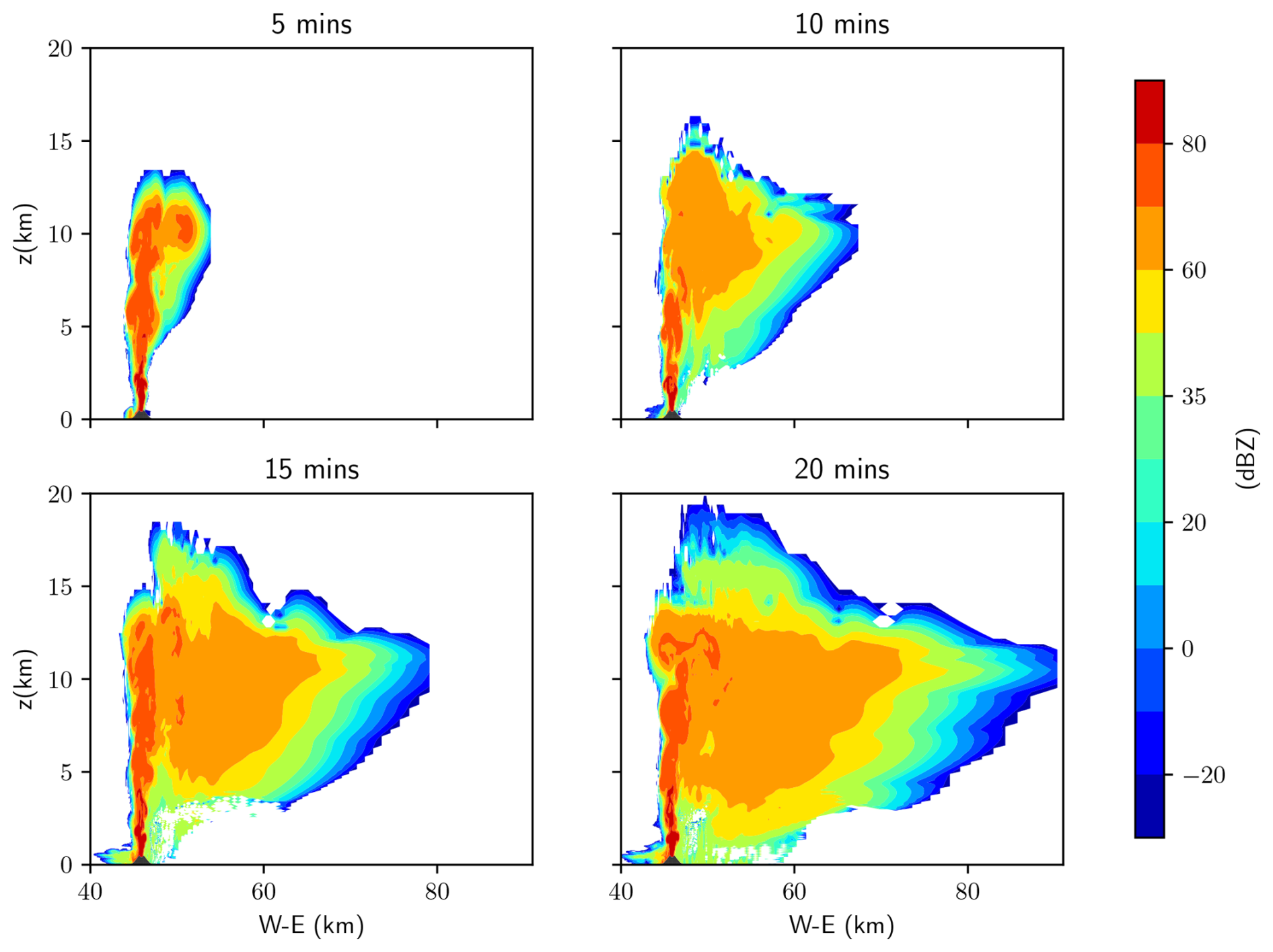
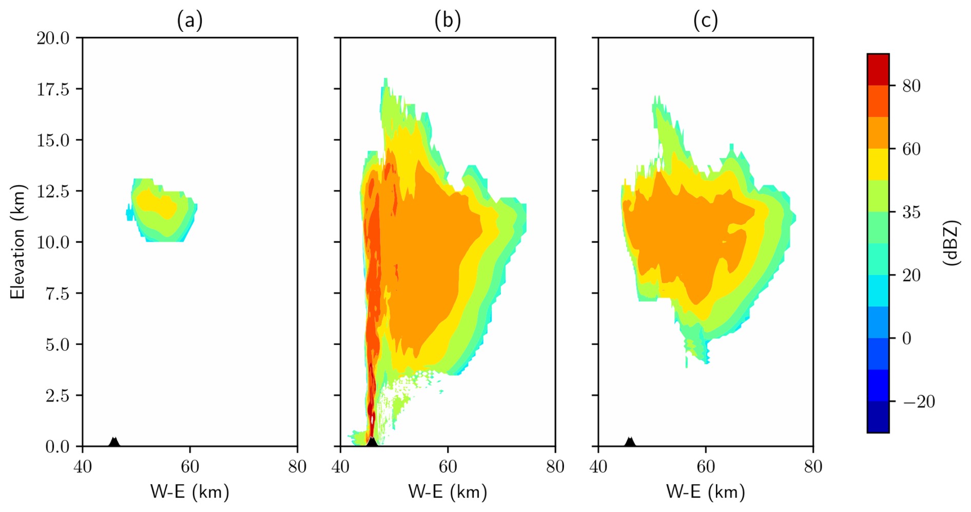
Figure 2 Equivalent radar reflectivities (Z_e) calculated using the Mie theory of the total scattering cloud (ash + hydrometeors) every 5 min following the eruption. The figure shows Z_e at a vertical cross-section across the vent.

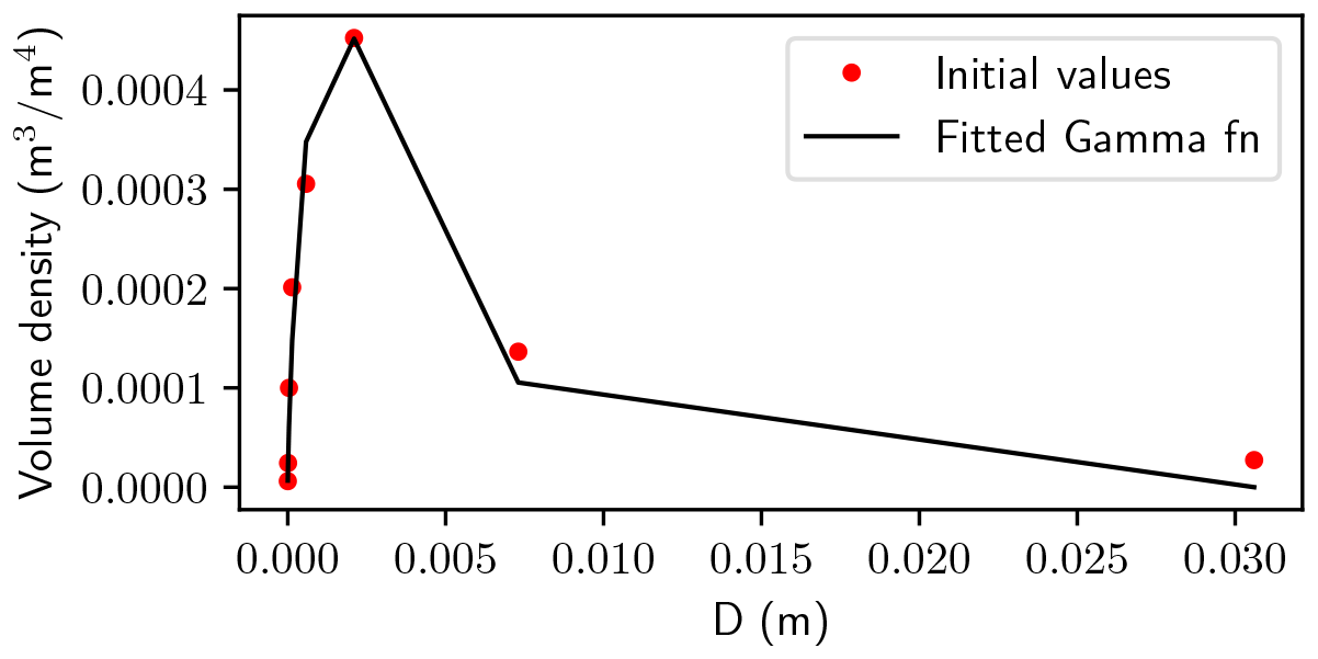
Figure 3 Initial volume density (the volume of ash particles for each size bin) for ash (red dots). The black line shows the fit to the volume density.

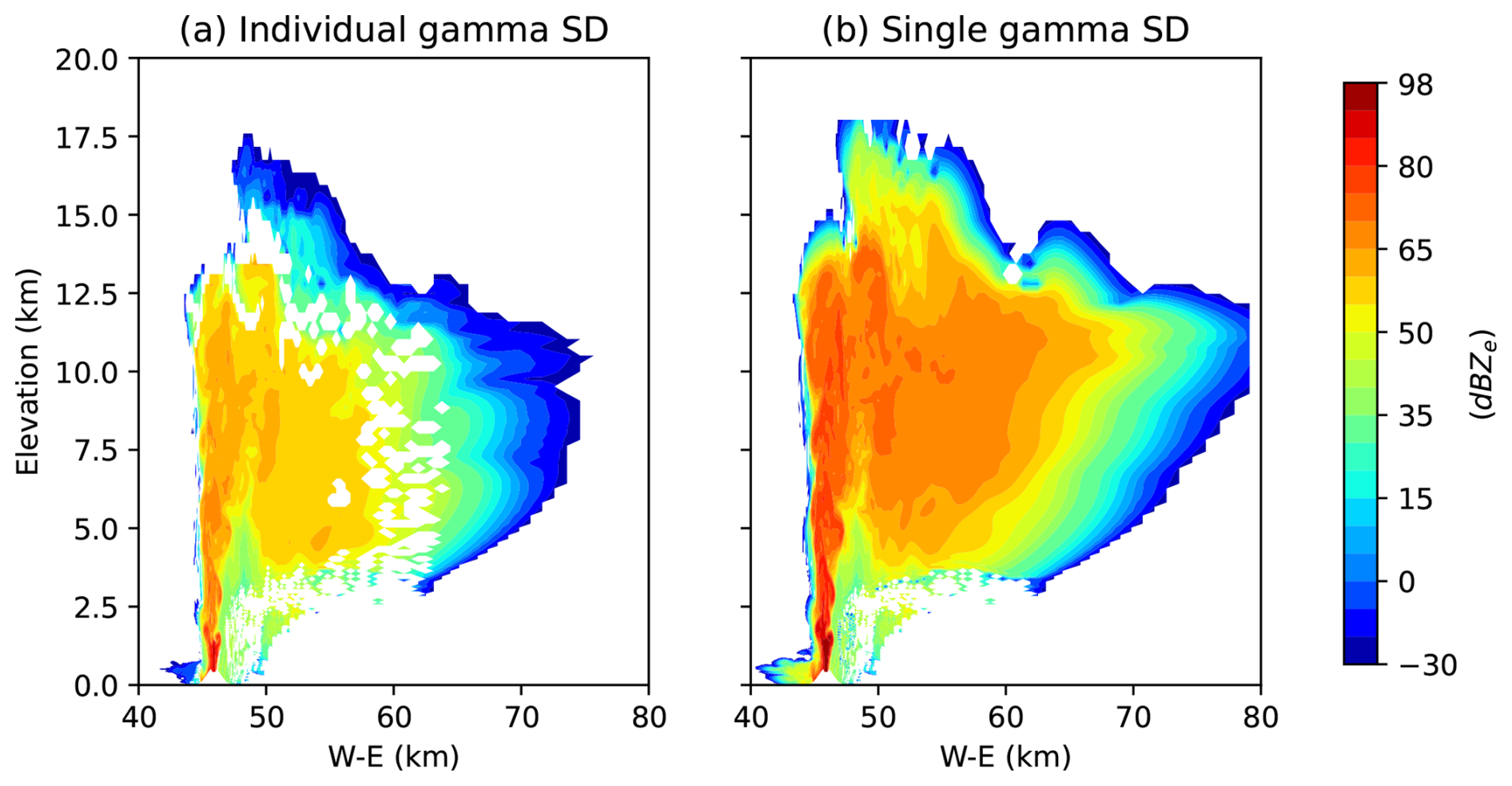
Figure 4 Equivalent radar reflectivities at a west–east cross-section at the vent at t=15 min post-eruption. The two plots show Z_e with (a) the superposition of separate gamma distributions for each ash category and (b) one single gamma function to represent the entire size distribution of ash.

The radar reflectivity module is used to calculate Z_e at different times following the eruption and is shown as a cross-section across the vent in Fig. 2. The plume reaches a maximum height of almost 20 km within 15 min. We choose the results at t=15 min to showcase the ability of SynRad to capture the characteristics of the volcanic plume in the following section.

4.2 Results

Three key outputs from the radar reflectivity module are the equivalent radar reflectivity (Z_e) values; the vertical maximum intensity (VMI) or the composite reflectivity, which is calculated as the maximum Z_e (dBZ) in each vertical column; and the radar echo top, which is the maximum cloud-top height in each vertical column. These fields are chosen because they are the commonly seen operational radar images. For SynRad calculations, we only consider grid points with total specific concentrations (of ash and hydrometeors) greater than 10⁻⁸ kg kg⁻¹. This is to reduce the computational time, as signals from range cells with concentrations below this threshold are guaranteed to be below the MDS and, hence, not detected by the radar. Once the return signal P_r is calculated for each of these grid points, a threshold (equal to the MDS for a corresponding radar) is applied on the P_r field to remove all return signals less than the MDS. Then, the maximum value of Z_e and the cloud top in each of these vertical columns gives the SynRad-obtained VMI and the echo top, respectively.

In this section, these fields from SynRad will be compared with the ATHAM output. For this, ATHAM output is first converted to comparable fields. Figure 5 shows the maximum plume heights (panel a) and VMIs (panel c) calculated from ATHAM output at t=15 min. To calculate the maximum plume heights, a threshold of 2 × 10⁻⁴ g m⁻³ is applied to the total concentration (ash + hydrometeors) fields in ATHAM, and the highest point in each vertical column with concentrations above this threshold is identified. This threshold is chosen because it is the concentration limit at which “enhanced procedures” are to be implemented by airlines due to the danger that ash poses to the aircraft jet engines (Kelleher, 2010). To calculate the ATHAM VMIs, the specific concentrations are converted to equivalent radar reflectivity (Z_e) values using Eq. (16). The VMI is then the maximum of these dBZ_e values in each vertical column. The ATHAM VMIs are calculated at each grid point and, hence, do not include any effects of attenuation. In essence, the difference between the ATHAM and SynRad values for both VMI and echo tops will be due to the attenuation experienced by the radar signal in SynRad.

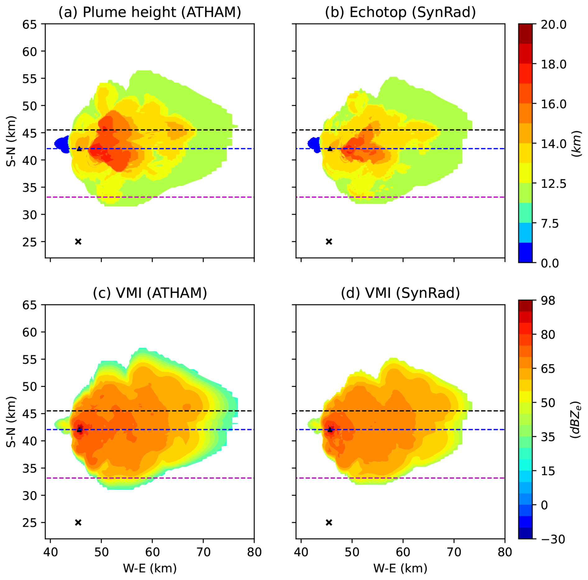
Figure 5 Comparison of ATHAM and SynRad results. The fields under comparison are the (a) ATHAM plume-top height calculated from simulated tracer concentrations, (b) SynRad echo top, (c) ATHAM maximum radar reflectivity values in a vertical column, and (d) SynRad VMI at t=15 min. The vent location is represented by the triangle, while the cross denotes the position of the radar. The ATHAM plume heights are calculated as the highest point in a vertical column with a total concentration greater than or equal to 2 × 10⁻⁴ g m⁻³, whereas SynRad echo tops are the highest point in a vertical column from which a return signal is detected. The dashed lines represent the three different west–east cross-sections, the results of which will be shown in following figures. These are locations before the vent (dashed pink line), at the vent (dashed blue line), and behind the vent (dashed black line).

At t=15 min, SynRad captures most of the ash cloud (as shown in Fig. 5). Following the meteorological conditions of the day, the ash cloud is dispersed to the east and spreads to the north, with cloud heights varying from a maximum of approximately 20 km closer to the vent to approximately 10 km in the distal ash cloud at x=80 and y= 30 km. The cloud echo tops or the radar-indicated cloud top near the vent detected by the C-band radar as calculated by SynRad (Fig. 5b) is less than the maximum plume heights of the ATHAM cloud (Fig. 5a). Using the ash concentrations (in kg m⁻³) of the individual categories, we calculated the maximum plume heights of each ash category (results are shown in Fig. 6). This analysis revealed that the first four ash categories (D= 2–140 µm; Fig. 6a–d) dominate the maximum plume height field in Fig. 5a. The maximum plume heights for the four larger-ash categories (Fig. 6e–h) are well below those of the finer-ash clouds. The C-band radar cannot detect the fine-ash cloud (the first four categories in this case), especially close to the vent (orange and red cloud), or the distal cloud (light-green cloud). This could be because of the attenuation due to the presence of larger ash (near the vent) in the signal path or the lower concentrations leading to a weaker return signal (in the distal cloud) from the four smaller-ash categories. This will be explored in detail later in the section.

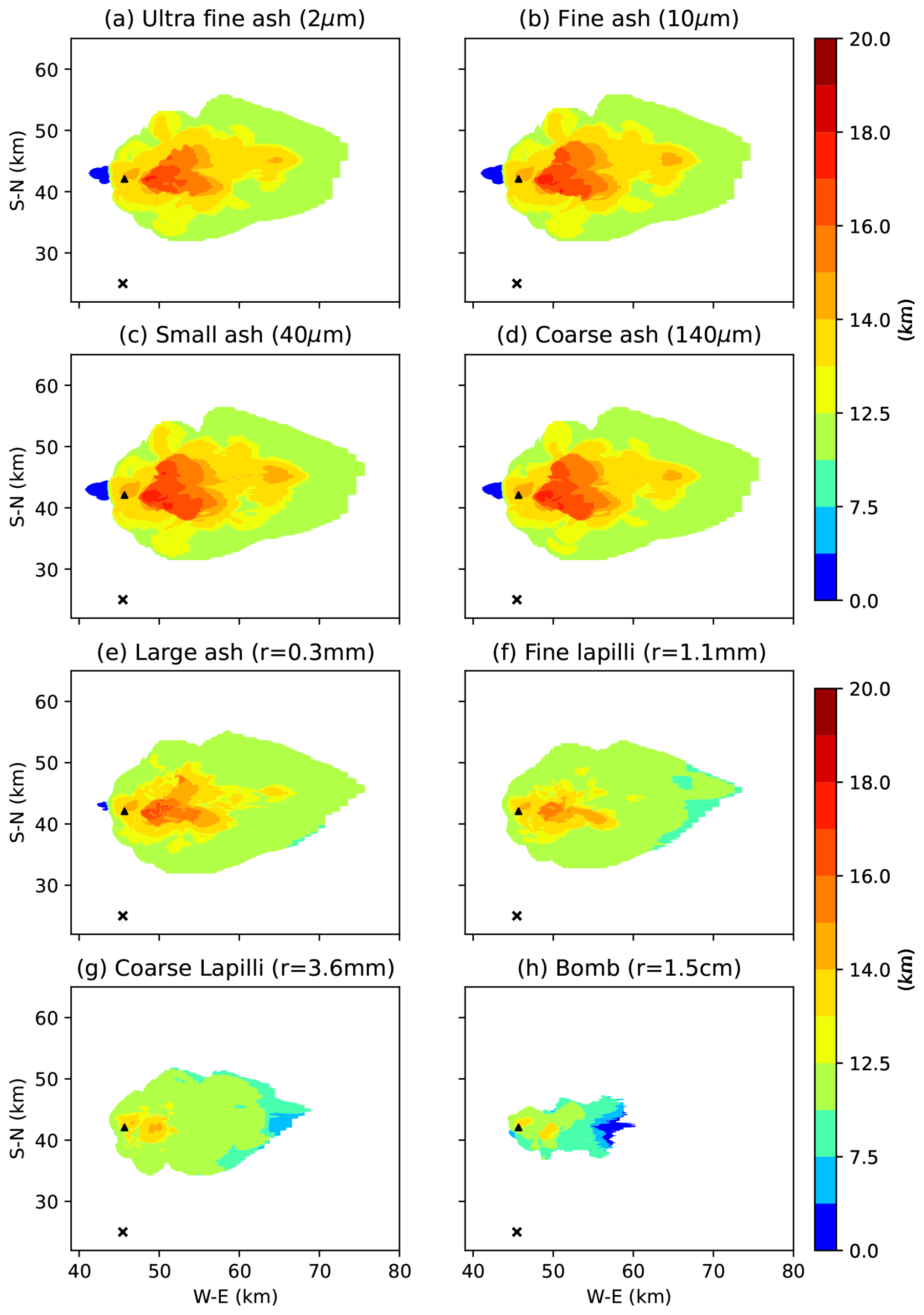
Figure 6 Plume heights calculated from ATHAM data at t=15 min for individual ash categories by applying a threshold of 2 × 10⁻⁴ g m⁻³ on individual ash concentrations.

The VMIs are a measure of the reflectivities of the larger and highly scattering particles, and there is a very good agreement between Fig. 5c and d, especially closer to the vent (and even in the distal cloud). The VMIs shown in Fig. 5c are completely dominated by the ash particles, as the maximum reflectivities of the hydrometeors are always less than those of the larger ash particles. Even within ash, certain categories are preferentially detected by the radar. The reflectivity contribution from total ash concentrations in one cell is calculated by assuming that the size distributions follow one single gamma distribution (as detailed in Sect. 4.1.1). An analysis to calculate the individual ash category contributions to the VMI field was performed by numerically splitting the ash size distribution into eight different size ranges (with each size in Table 2 assumed to be the centre of the bin). This revealed that the first four ash categories (D= 2–140 µm) have maximum reflectivities well below −30 dBZ and, hence, do not have a significant contribution to the total ash volumetric reflectivity. As discussed earlier, this means that these categories are not detected by the radar. On the other hand, the relatively large wavelength of the C-band radar also means that it is likely to preferentially detect the high-reflectivity tephra (i.e. the larger-ash categories) and hydrometeors, and this ultimately decides the VMI values. Comparing Fig. 5c to the VMIs of the larger-ash categories (Fig. 7), it is likely that the radar preferentially detects the coarse lapilli. In the Rayleigh regime, there is an almost linear increase in the particle radar cross-sections with diameter, and this increase then plateaus once the Mie regime is reached. For a particular ash category to lie in the Rayleigh or Mie regime, the size parameter $x=\mathrm{2}\mathit{\pi }r/\mathit{\lambda }$ should be much less than 1. The values of this parameter, given in Table 2, reveal that the last ash category (bombs) falls in the Mie regime. This explains why the coarse lapilli have a stronger return signal than the bombs, which are larger in size. At the distal cloud, the C-band radar fails to detect the ash particles (shades of light green in Fig. 5d), which dominate the maximum reflectivities at these distances (as is also apparent in the echo tops) in Fig. 5. At these distances, the four larger-ash categories are usually present in smaller concentrations, with the VMIs dominated by the finer-ash cloud (which is undetected), leading to the difference between the two figures at these low reflectivities. Moreover, the radar fails to capture the high-reflectivity region east of the vent (50–60 km along the x axis) in Fig. 5c. As will be shown in Fig. 8, the radar signal is attenuated, resulting in a weaker signal in this region.

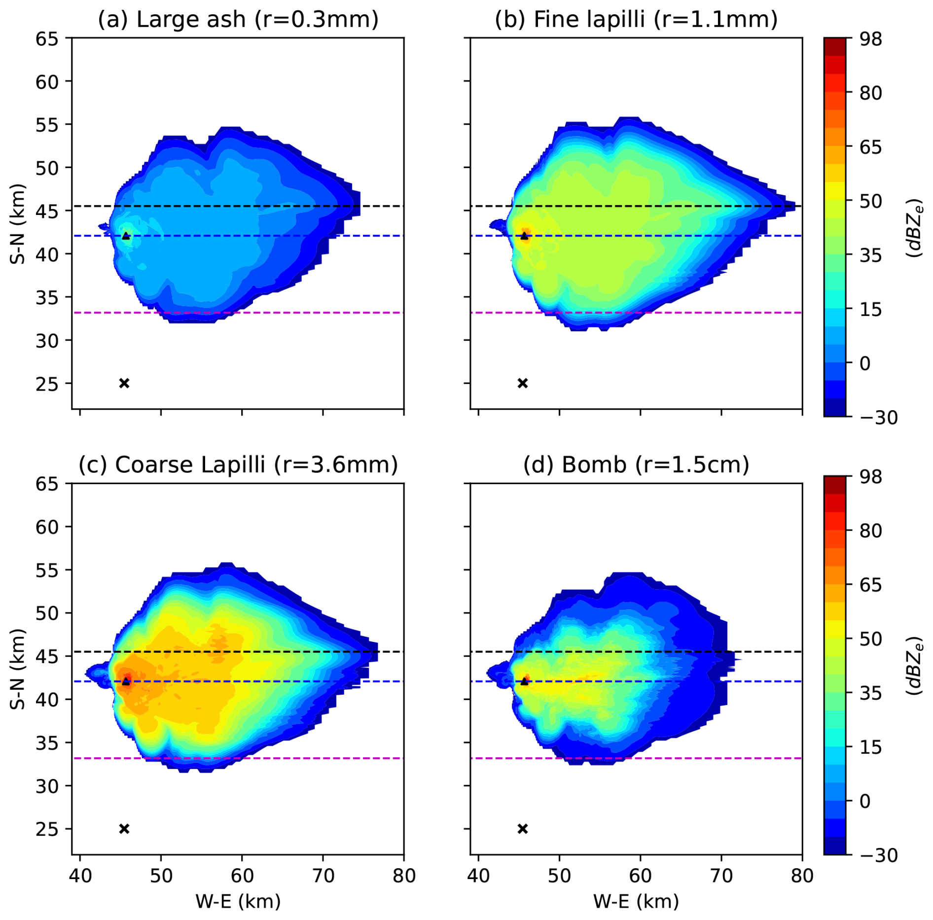
Figure 7 VMI fields calculated from ATHAM data at t=15 min for (the four largest) individual ash categories. The VMIs for the four smaller categories (not shown) are well below the −30 dBZ threshold imposed in this study. The dashed lines are the same as in Fig. 5.

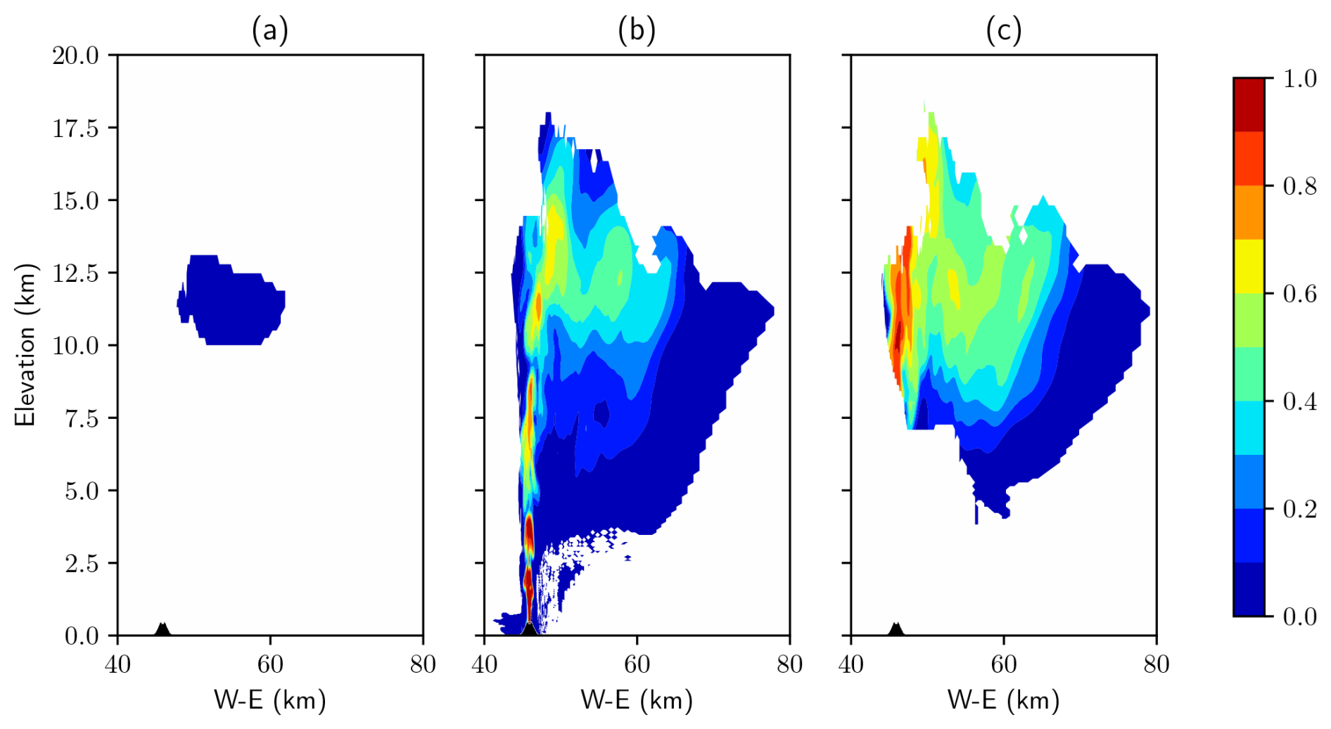
Figure 8 Signal attenuation (unitless) calculated by the ray-tracing module of SynRad at three different west–east cross-sections in the numerical domain at t=15 min: (a) before the vent (dashed pink line in Fig. 5), (b) at the vent (dashed blue line in Fig. 5), and (c) behind the vent (dashed black line in Fig. 5).

The path attenuation (from the radar location to the vent) experienced by the C-band radar due to the ash and hydrometeors is investigated next in Fig. 8 at three cross-sections (represented in Fig. 5 as dashed lines). Figure 8a, b, and c are cross-sections corresponding to the pink, blue, and black dashed lines in Fig. 5, respectively. These cross-sections are selected to study the effect of attenuation at different locations relative to the vent and radar location. The first line (pink) corresponds to a location 9 km in front of the vent, where we expect only finer ash and, hence, lower attenuation; the second line (blue) is at the vent, where we expect larger tephra; and the third line (black) is a location 3.4 km behind the vent, where the rays will have had to pass through a significant amount of attenuating ash cloud. The colour bars range from 0 to 1, indicating a non-attenuated and fully attenuated signal, respectively. Figure 8a shows no to minimal path attenuation. At this cross-section, even though the radar rays are travelling through all of the ash categories, the reflectivities of the four bigger-ash categories are well below zero, which results in no or negligible attenuation in the C-band. At a cross-section across the vent (Fig. 8b), heavy attenuation is seen vertically above and close to the vent. This is the attenuation experienced by the radar ray when it travels through the small region around the vent with very large and coarse tephra. The category-wise split of the VMIs reveals that the region of high reflectivity most responsible for the attenuation is actually the coarse lapilli (category 7), as they are present in a higher concentration than the larger bombs (category 8). This is the dark-red patch around the vent in Fig. 5c with reflectivities above 80 dBZ. This patch of tephra with high reflectivities is also responsible for the high extinction of the signal (slender red column) in Fig. 8c. The cross-section in between these two locations reveals a similar pattern (not shown), with the slender red region stretching from the vent to altitudes up to 15 km (as in Fig. 8c). The broader attenuation experienced by the signal up to 65 km east in Fig. 8b and c is from when the beam passes through the high-reflectivity region (> 60 dBZ shown in orange/dark yellow).

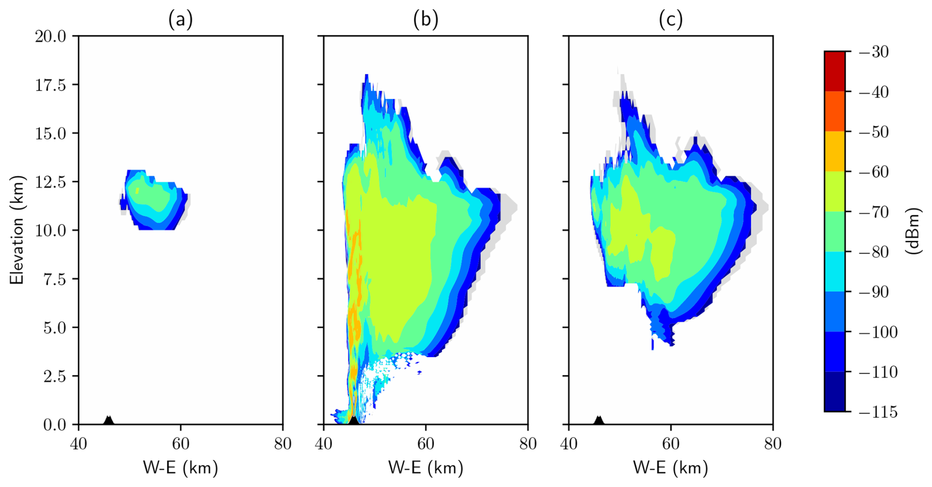
The return power P_r (dBm) from each radar gate is presented in Fig. 9. The grey halo around the ash clouds represent the actual cloud from ATHAM data. These are all points with total specific concentrations greater than 10⁻⁵ g kg⁻¹, i.e. all points that we are calculating return signals from, as mentioned at the start of the section. Most of the ash cloud in Fig. 9a is made up of high-reflectivity tephra and hydrometeors, as is evident in Fig. 10a, where the minimum reflectivity in the cloud is around 20 dBZ. This, combined with the negligible path attenuation experienced by the beam up to this cross-section and the relative closeness of the radar to the target volume, results in a return signal that is above the MDS of the C-band radar. Figure 9b, however, reveals a counter-intuitive picture. As the signal undergoes a degree of path attenuation, as revealed by Fig. 8b, we expect a weak signal from the slender column experiencing the heavy attenuation and the return power to reflect the attenuation cross-section. However, we see a stronger signal than expected in the slender column. This is due to a combination of two facts: (1) even though the signal is heavily attenuated, it is not fully extinguished (hence, the value of attenuation does not drop to zero); (2) the slender column possibly has the largest tephra (in addition to particles of all sizes) and the high-reflectivity tephra, resulting in a high return signal even when multiplied by the attenuation value (as in Eq. 7). This results in the return power signal cross-sections closely mirroring the cross-sections of the equivalent radar reflectivities Z_e (Fig. 10) rather than the cross-sections for the attenuation. We believe that, for an eruption that results in tephra of smaller size categories or for a radar of higher frequencies (where the signal is completely attenuated to zero), the return power signal cross-sections will closely mirror the attenuation cross-sections. This theme is also followed in Fig. 9c, with the cross-section further behind the vent revealing a return signal that is in contradiction to the attenuation cross-section. However, another interesting feature in this figure is the more obvious appearance of the grey halo, suggesting that this frequency band does not capture the outer bands of the ash cloud. Comparison with the attenuation figure suggests that this is not due to the signal being attenuated but rather due to the range and the fact that we tend to have lower concentrations of fine (smaller in size) ash at these distances, leading to the return signal at the radar from these distances being lower than the MDS.

Figure 9 The return signal power (P_r, in dBm) calculated by SynRad at three different west–east cross-sections: (a) before the vent (dashed pink line in Fig. 5), (b) at the vent (dashed blue line in Fig. 5), and (c) behind the vent (dashed black line in Fig. 5).

Figure 10 Equivalent radar reflectivities (dBZ) calculated by SynRad at three different west–east cross-sections: (a) before the vent (dashed red line in Fig. 5), (b) at the vent (dashed blue line in Fig. 5), and (c) behind the vent (dashed black line in Fig. 5).

5 Summary

A recently developed radar forward operator, SynRad, which simulates the measurement process of a scanning weather radar and generates synthetic radar signals from 3D output from volcanic plume models is presented. It simulates key scanning weather radar observables like equivalent radar reflectivity, path attenuation, return signals, vertical maximum intensities, and echo tops. The operator is specially designed to simulate the measurement processes behind the detection of volcanic clouds using scanning weather radars, for which attenuation due to volcanic ash is key to deciding how deep into the ash cloud the signal can penetrate. Also considered is the scattering or attenuation due to hydrometeors, such as cloud droplets, raindrops, ice crystals, and graupel. SynRad produces return signals from each grid point in the 3D output that it is working on. A key feature of this operator is the ray-tracing module that tracks radar beams from the antenna to the cloud (and back) and calculates the attenuation along its path. The high computational cost of the ray-tracing module leads us to opt for certain simplifications, such as assuming that the radar beam propagates as a single ray to each grid cell (rather than assuming the actual volume of the beam). We also ignore attenuation due to any gases in the atmosphere or within the ash cloud, the Doppler observations, and beam bending, and we assume the radar to be a single-polarization radar.

The 2019 eruption of the Raikoke volcano is used as the case study to showcase the capabilities of SynRad. The measurement process of a C-band scanning weather radar is simulated, and the equivalent reflectivities, VMIs, and echo tops are calculated. The operator was able to generate realistic fields of the equivalent radar reflectivities, and the echo tops and VMIs from SynRad show good agreement with those generated from ATHAM.

SynRad can be used to identify the best possible locations for operationally deploying radar to monitor the ash cloud following an eruption. Locations can be identified that allow maximum penetration into and, hence, detection of the ash cloud. Another key prospective application is that SynRad can possibly be used to identify the optimal frequency or frequencies (for a multi-frequency radar) that balance the trade-off between a higher return signal and the higher path attenuation that comes at these higher frequencies. This will be the focus of a follow-up paper. In addition, the synthetic radar signals can be used to develop and test radar retrieval algorithms for the retrieval of ash properties, including their mass and size. SynRad can also be used in the context of verifying the cloud microphysics implemented in any plume model. This can be done by comparing the radar observables calculated from the prognostic cloud model variables and directly comparing radar observables with weather radar observables. The operator can also be used to assimilate radar data into prediction models. An estimate of the eruption source parameters (such as ash concentrations and size) can be arrived at by combining a prior forecast state with the observations/radar observables from the operator, which can then be used as an initial state of the volcanic ash transport and dispersion models.