Enhancing winter climate simulations of the Great Lakes: insights from a new coupled lake–ice–atmosphere (CLIAv1) system on the importance of integrating 3D hydrodynamics with a regional climate model

The Laurentian Great Lakes significantly influence the climate of the Midwest and Northeast United States due to their vast thermal inertia, moisture source potential, and complex heat and moisture flux dynamics. This study presents a newly developed coupled lake–ice–atmosphere (CLIAv1) modeling system for the Great Lakes by coupling the National Aeronautics and Space Administration (NASA) Unified Weather Research and Forecasting (NU-WRF) regional climate model (RCM) with the three-dimensional (3D) Finite Volume Community Ocean Model (FVCOM) and investigates the impact of coupled dynamics on simulations of the Great Lakes' winter climate. By integrating 3D lake hydrodynamics, CLIAv1 demonstrates superior performance in reproducing observed lake surface temperatures (LSTs), ice cover distribution, and the vertical thermal structure of the Great Lakes compared to the NU-WRF model coupled with the default 1D Lake Ice Snow and Sediment Simulator (LISSS). CLIAv1 also enhances the simulation of over-lake atmospheric conditions, including air temperature, wind speed, and sensible and latent heat fluxes, underscoring the importance of resolving complex lake dynamics for reliable regional Earth system projections. More importantly, the key contribution of this study is the identification of critical physical processes that influence lake thermal structure and ice cover – processes that are missed by 1D lake models but effectively resolved by 3D lake models. Through process-oriented numerical experiments, we identify key 3D hydrodynamic processes – ice transport, heat advection, and shear production in turbulence – that explain the superiority of 3D lake models to 1D lake models, particularly in cold season performance and lake–atmosphere interactions. Critically, all three of these processes are dynamically linked to water currents – spatially and temporally evolving flow fields that are structurally absent in 1D models. This study aims to advance our understanding of the physical mechanisms that underlie the fundamental differences between 3D and 1D lake models in simulating key hydrodynamic processes during the winter season, and it offers generalized insights that are not constrained by specific model configurations.

1 Introduction

The Laurentian Great Lakes, with a surface area of 246 000 km², represent Earth's largest surface freshwater resources, containing 21 % of the world's surface freshwater and 84 % of North America's surface freshwater (EPA, 2014; Notaro et al., 2015; Xue et al., 2022). Over 55 million people live within the Great Lakes megaregion (Todorovich, 2009; Sharma et al., 2018). The lakes support the United States and Canadian economies by impacting drinking water supply and through shipping, fishing, power production, transportation, manufacturing, wastewater treatment, agriculture, and recreation (Vaccaro and Read, 2011). The Great Lakes' support of these vital industries sustains approximately 1.3 million jobs and USD 82 billion in annual wages (Rau et al., 2020). As an invaluable resource for wildlife and society, the ecologically diverse Great Lakes Basin is home to over 3500 animal and plant species, including over 170 fish species (Crossman and Cudmore, 1998; EPA, 2014). The basin's wetlands serve as spawning and nesting habitats, reduce erosion, and protect water quality (Notaro et al., 2015).

The Great Lakes are critically important in terms of their impacts on the climate of the Midwest and Northeast United States and southern Ontario, Canada. The regional climate is highly sensitive to the Great Lakes due to their vast thermal inertia, potential source of moisture to the overlying atmosphere, and contrasts in heat, moisture, roughness, and albedo compared to the surrounding land (Changnon and Jones, 1972; Scott and Huff, 1996; Chuang and Sousounis, 2003; Notaro et al., 2013a; Bryan et al., 2015; Briley et al., 2021; Wang et al., 2022; Hutson et al., 2024). From late fall through winter, when cold, dry continental air masses from Canada pass over the relatively mild Great Lakes, the air masses are destabilized and moistened, leading to enhanced cloud cover and precipitation downwind of the lakes (Niziol et al., 1995; Ballentine et al., 1998; Kristovich and Laird, 1998; Notaro et al., 2013b; Shi and Xue, 2019). During the broader unstable lake season, which lasts from September to March and is characterized by amplified lake-effect cloud cover and precipitation due to lake surface temperatures typically exceeding overlying air temperatures, lake-effect snowfall typically peaks during December–January, and lake ice cover is most extensive during February–March (Assel, 1990; Niziol et al., 1995; Kristovich and Laird, 1998; Notaro et al., 2013b). The establishment of extensive lake ice cover, usually by midwinter to late winter, dampens over-lake turbulent fluxes of heat and moisture, subsequently reducing the resulting lake-effect precipitation (Brown and Duguay, 2010; Notaro et al., 2021). Specifically, increasing lake ice cover leads to a linear reduction in latent heat fluxes and nonlinear reduction in sensible heat fluxes (Gerbush et al., 2008). When relatively cool (warm) air masses pass over the Great Lakes during winter (summer), the relatively warm (cool) lake surface reduces (enhances) atmospheric stability and increases (decreases) deep convection, cloud cover, and precipitation (Scott and Huff, 1996; Holman et al., 2012; Bennington et al., 2014). The lakes' relatively low roughness compared to the surrounding land leads to strengthened over-lake wind speeds and potential shoreline convergence in support of enhanced lake-effect precipitation. Due to the lakes' large thermal inertia and the resulting seasonal evolution in lake–air temperature contrast, the Great Lakes typically strengthen wintertime cyclones and summertime anticyclones and weaken summertime cyclones and wintertime anticyclones (Notaro et al., 2013a). The basin is a preferred zone of wintertime cyclogenesis due to the relative warmth of the lake surfaces and consequential enhancement of low-level convergence (Petterssen and Calabrese, 1959; Colucci, 1976; Eichenlaub, 1978).

Given the aforementioned substantial influence of the Great Lakes on regional climate, their representation and evaluation in both global and regional climate models have been the focus of several studies in the past decade. There is a wide spectrum of climate models regarding the treatment of large lakes. Due to their coarse spatial resolution, most global climate models (GCMs), including those from various phases of the Coupled Model Intercomparison Project (CMIP), either omit the Great Lakes entirely or offer a crude representation using wet soil, wetlands, ocean grid cells, or one-dimensional (1D) lake models (Briley et al., 2021; Minallah and Steiner, 2021).

Among regional climate models (RCMs) without lake models, many apply a rudimentary approach to estimating lake surface temperatures (LSTs) by extrapolating the closest ocean grid cell's sea surface temperatures (SSTs), likely from Hudson Bay or the North Atlantic Ocean, from the initial and lateral boundary condition datasets to the lake grid cell, potentially inducing vast biases and intra-lake discontinuities in LSTs and ice cover (Gao et al., 2012; Mallard et al., 2015; Bryan et al., 2015; Spero et al., 2016; Hanrahan et al., 2021). This approach is the default treatment of LSTs in the Weather Research and Forecasting (WRF) model (Hanrahan et al., 2021; Wang et al., 2022). Alternatively, the WRF Preprocessing System can designate time-averaged 2 m air temperatures to the underlying lake surfaces to provide estimated lower-boundary conditions of LSTs based on the user-specified time window for temporal averaging and time lag for addressing thermal inertia (Mallard et al., 2015; Hanrahan et al., 2021; Wang et al., 2022). However, this approach still produces unrealistic LSTs and ice cover as the lakes cannot achieve equilibrium with the overlying atmosphere due to the lack of interactive lake–atmosphere feedbacks (Bullock et al., 2014; Spero et al., 2016).

For those GCMs and RCMs that aim to incorporate coupled lake–atmosphere interactions, most apply 1D lake models (Perroud et al., 2009; Martynov et al., 2010; Stepanenko et al., 2010; Subin et al., 2012). These include two-layer bulk models founded in similarity theory such as the Freshwater Lake (FLake) model (Mironov et al., 2010), thermal diffusion models which parameterize eddy diffusivity such as the Minnesota Lake Water Quality Management Model (MINLAKE, Riley and Stefan, 1988) and the Hostetler model (Hostetler and Bartlein, 1990), Lagrangian turbulence models such as the Dynamics Reservoir Simulation Model (DYRSM, Yeates and Imberger, 2003), and k−ϵ turbulence closure models with horizontally averaged velocity such as LAKE (Stepanenko and Lykossov, 2005; Stepanenko et al., 2011) and Simstrat (Goudsmit et al., 2002). Each of these different categories of 1D lake models has its own advantages and disadvantages (Perroud et al., 2009; Martynov et al., 2010; Stepanenko et al., 2010; Subin et al., 2012). As demonstrated in these studies, the deficiencies include struggles with simulating seasonal stratification in FLake, insufficient mixing for deep lakes in the Hostetler model, and excessive mixing for shallow lakes in the computationally expensive turbulence models.

Multiple modeling studies have assessed the performance of coupling RCMs to 1D lake models in the Great Lakes region. While this coupling permits the representation of key lake–atmosphere interactions and the heterogeneous spatiotemporal patterns of LSTs and lake ice cover, 1D lake models typically perform poorly at reproducing the lake thermal structure and seasonal ice evolution of large, deep lakes, such as Lake Superior, due to the overly simplified hydrodynamic processes. Common biases in 1D lake models include anomalously early timing of both spring–summer stratification and fall turnover, with positive biases in summer LST and negative biases in winter LST (Bennington et al., 2014; Mallard et al., 2014). The International Centre for Theoretical Physics (ICTP) Regional Climate Model version 4 (RegCM4), coupled to the 1D Hostetler lake model, yields a prolonged lake ice season with excessive ice cover due to the neglect of horizontal heat advection within the lakes (Notaro et al., 2013b). The coupling of a thermal diffusion lake model, the Lake, Ice, Snow and Sediment Simulator (LISSS, Subin et al., 2012), to the WRF model (available starting with version 3.6 of WRF) results in an early warm-up and overly rapid cool-down in the seasonal evolution of LSTs for deep lakes, along with an early onset of lake ice cover in support of its excessive abundance (Xiao et al., 2016). Mallard et al. (2014) found that WRF, coupled to FLake, produced the best performance for Lake Erie (the smallest and shallowest Great Lake) and the worst performance for Lake Superior (the largest and deepest Great Lake) of the Great Lakes in terms of simulated LST and ice cover biases. Often, modelers aim to reduce biases in the simulated vertical temperature profile of deep lakes in 1D models by artificially enhancing the vertical eddy diffusivity to crudely compensate for the absence of a dynamic circulation and vertical mixing processes (Subin et al., 2012; Bennington et al., 2014; Lofgren, 2014; Gu et al., 2015; Mallard et al., 2015), although such a non-physics-based approach may only yield limited benefits to minimizing these biases (Xiao et al., 2016). The lack of fully resolved lake hydrodynamics in models (Xue et al., 2017; Sharma et al., 2018), including lake circulation (Song et al., 2004), upwelling and downwelling, thermal bar formation (Martynov et al., 2010, 2012), explicit horizontal mixing, and ice motion, along with overly simplified stratification processes (Bennington et al., 2014) and unrealistic treatment of eddy diffusivity (Stepanenko et al., 2010; Gu et al., 2015; Mallard et al., 2015), has been the main obstacle to further improving climate simulations for the Great Lakes Basin.

In recent years, a limited number of studies on the Great Lakes and other large inland seas have sought to enhance the representation of 3D lake hydrodynamical processes and reduce the substantial biases in LST and ice cover associated with 1D lake models by coupling RCMs with 3D hydrodynamic models (Turuncoglu et al., 2013; Xue et al., 2017, 2022; Sun et al., 2020; Kayastha et al., 2023). These studies have responded to the urgent call for continued progress in coupling high-resolution RCMs with 3D lake models that address the complex processes and features of large, deep lakes, as highlighted in previous research (Martynov et al., 2010; Bennington et al., 2014; Briley and Jorns, 2021; Leon et al., 2005, 2007; Bryan et al., 2015; Notaro et al., 2021). Xue et al. (2017) developed a two-way-coupled 3D lake–ice–climate modeling system, known as the Great Lakes-Atmosphere Regional Model (GLARM), by coupling RegCM4 with a 3D unstructured-grid hydrodynamic model, the Finite Volume Community Ocean Model (FVCOM, Chen et al., 2012). The resulting coupled 3D modeling system exhibited notable skill in reproducing the mean, variability, and trends in regional climate across the Great Lakes Basin and the physical characteristics of the Great Lakes, including their thermal structure and ice cover, significantly improving upon previous RCM experiments coupled with 1D lake models. The updated version, GLARM-V2, has been utilized to generate future climatic and limnological projections for the Great Lakes region (Xue et al., 2022). Similarly, Sun et al. (2020) developed a lake–atmosphere–hydrology modeling system by coupling the Climate-WRF (CWRF) model with the 3D FVCOM and compared its performance against that of CWRF coupled with the 1D LISSS. They found that the former configuration outperformed the latter in simulating LST, ice cover, and the vertical thermal structure in the Great Lakes. Kayastha et al. (2023) developed and validated the WRF-FVCOM Two-way Coupling (WF2C) model, showing that WF2C improved upon past 1D lake-model-based studies by significantly reducing the simulated summer LST bias and revealing how coupled lake–atmosphere dynamics can influence summer LST by modifying surface heat fluxes through impacts on meteorological state variables. These studies underscore the advantages of coupling an RCM with a 3D lake hydrodynamic model to accurately depict lake physical processes and lake–atmosphere feedbacks in the Great Lakes Basin. However, there is a notable absence of research dedicated to identifying the fundamental processes resolved in 3D lake models that contribute to these improvements, which is important for optimizing effort allocation in future model development and improving our predictive understanding of the system. This knowledge gap is particularly significant for the Great Lakes during the winter seasons.

This paper attempts to address this knowledge gap by developing a new coupled lake–ice–atmosphere (CLIA version 1 or CLIAv1) modeling system for the Great Lakes by coupling the National Aeronautics and Space Administration (NASA) Unified Weather Research and Forecasting (NU-WRF) RCM with the 3D FVCOM. Note that CLIAv1 is hereinafter referred to as NU-WRF/FVCOM for the sake of particular attention given to comparing NU-WRF's performance during the cold season when coupled two-way with the 3D FVCOM (NU-WRF/FVCOM) versus the 1D LISSS (NU-WRF/LISSS). After a thorough validation of the coupled model, we conduct a series of process-oriented numerical experiments to identify the most important hydrodynamic processes that contribute to the superiority of the 3D lake model to the 1D lake model in enhancing lake–atmosphere coupling for the Great Lakes.

2 Models and coupling approach

2.1 Atmospheric model

NU-WRF is an observation-driven integrated regional modeling system developed at NASA's Goddard Space Flight Center (GSFC) that resolves chemistry, aerosol, cloud, precipitation, and land processes at satellite-resolvable scales (roughly 1–25 km) to improve the continuity between microscale, mesoscale, and synoptic processes. Developed as a superset of the community WRF, NU-WRF unifies the NCAR Advanced Research version of the WRF model (WRF-ARW) with the GSFC Land Information System (LIS, Kumar et al., 2006; Peters-Lidard et al., 2007, 2015), the Goddard Chemistry Aerosol Radiation and Transport (GOCART) model (Chin et al., 2000), the Goddard radiation and microphysics schemes (Shi et al., 2014), and the Goddard Satellite Data Simulator Unit (G-SDU, Matsui et al., 2013, 2014). NU-WRF simulations here utilize the Noah Land Surface Model, which simulates soil moisture and temperature, skin temperature, snowpack depth, and the energy flux and water flux terms of the surface energy balance and surface water balance (Mitchell, 2005). Currently, by default, the two-way lake–atmosphere interactions in NU-WRF are represented using the embedded 1D LISSS (Subin et al., 2012) from the Community Land Model version 4.5 (Oleson et al., 2013), with modifications by Gu et al. (2015).

Notaro et al. (2021) conducted 20 simulations to identify the regionally optimal NU-WRF configuration and schemes for the cold season period of November 2014–March 2015 in the Great Lakes region. The best model configuration was referred to as the “Morrison combination” and is used in this study. The Morrison combination includes Morrison microphysics (Morrison et al., 2009), Rapid Radiative Transfer Model (RRTM, Mlawer et al., 1997) longwave radiation physics, Community Atmosphere Model (CAM, Collins et al., 2004) shortwave radiation physics, Mellor–Yamada–Nakanishi–Niino Level-2.5 (MYNN2.5, Nakanishi and Niino, 2006, 2009) planetary boundary layer physics, and Mellor–Yamada–Nakanishi–Niino (MYNN, Nakanish, 2001) surface layer schemes. The improved simulations of air temperature and surface insolation using the Morrison combination benefit primarily from the Community Atmosphere Model's shortwave radiation scheme (Notaro et al., 2021). The Morrison combination is essentially the WRF configuration determined by Mooney et al. (2013) to produce the best-simulated wintertime temperature simulation over Europe; they found that winter air temperatures are highly sensitive to the choice of radiation physics.

The NU-WRF one-way-nested configuration consists of an outer domain with 15 km grid spacing for the majority of North America and an inner domain with 3 km grid spacing for the Great Lakes region (Fig. 1), with the atmospheric vertical resolution assigned to 61 levels. The initial and lateral boundary conditions are provided by the Global Data Assimilation System 0 h analysis. The cumulus parameterization option used for the outer domain is the Kain–Fritsch scheme (Kain and Fritsch, 1990; Kain, 2004) with resolved, un-parameterized convection in the inner domain.

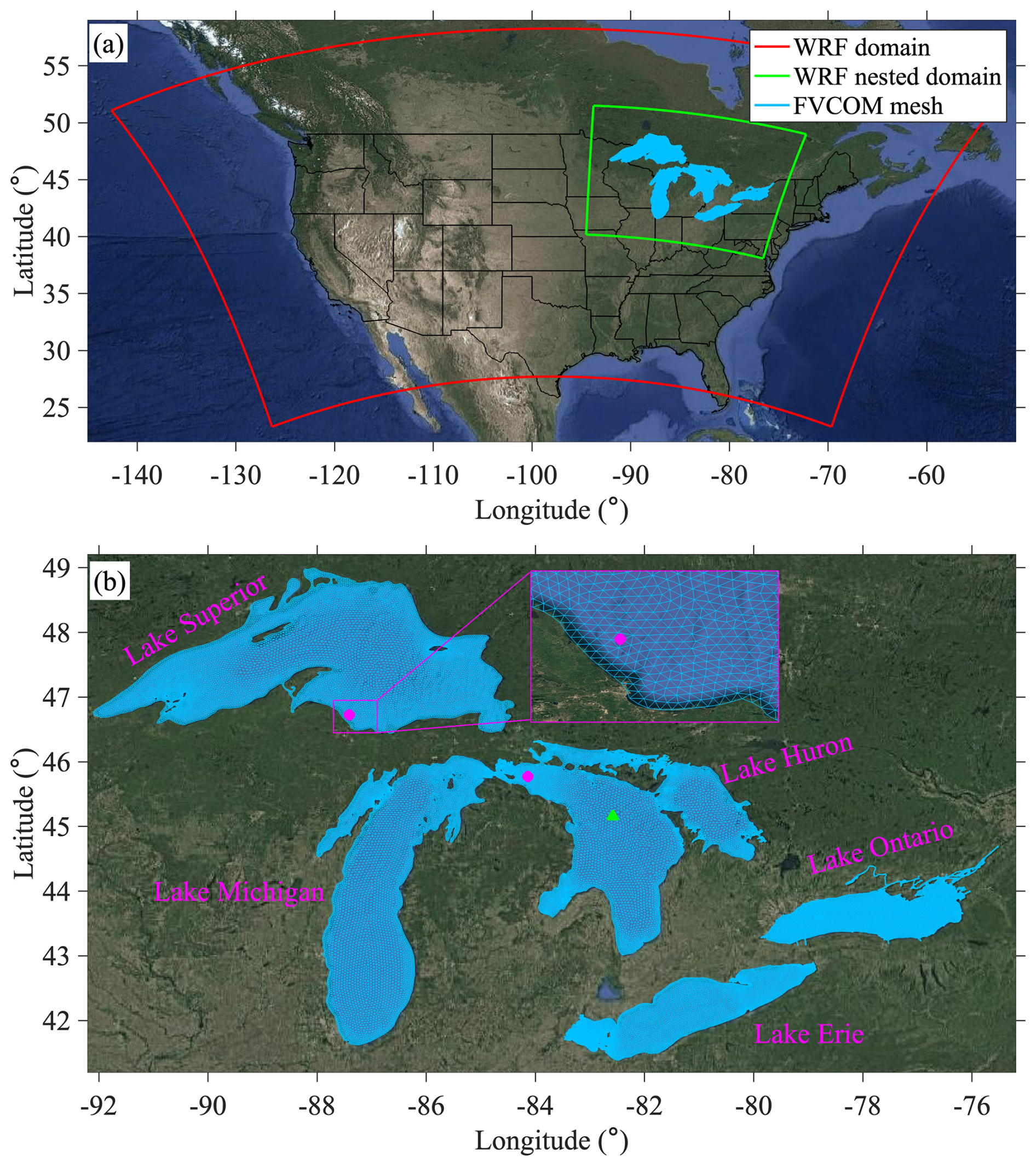
Figure 1 NU-WRF nested domains (a) and the unstructured mesh used in FVCOM to represent the Great Lakes in FVCOM (b). The two dots denote the locations of Granite Island (87.4° W, 46.7° N) on Lake Superior and Spectacle Reef (84.1° W, 45.7° N) on Lake Huron. The triangle marker denotes the location (82.58° W, 45.16° N) of the thermistor observation in the deep, central Lake Huron, where the water depth is 220 m.

2.2 The 3D hydrodynamic model

FVCOM is a free-surface, primitive-equation, and 3D hydrodynamic model that solves the momentum (3D currents), continuity (surface water elevation), temperature, salinity, and density equations and is closed physically and mathematically using turbulence closure submodels (Chen et al., 2012). The full formulation of the primitive equations used in FVCOM is provided in Chen et al. (2012; Eqs. 2.1–2.10). Numerically, FVCOM employs the finite-volume method over an unstructured triangular grid and vertical sigma layers, optimizing flexibility and accuracy for complex terrains. The grid resolution adjusts from 1–2 km near coasts to resolve coastal geometry complexity to 2–4 km offshore to improve computational efficiency (Fig. 1), with the model comprising 35 000 grid cells and 40 sigma layers. Vertical mixing processes are modeled using the Mellor–Yamada Level-2.5 (MY25) turbulence closure model (Mellor and Yamada, 1982), while horizontal diffusivity is derived from velocity shear and grid resolution through the Smagorinsky (1963) formulation.

2.2.1 Advective heat transport

When applied as a 3D lake model, FVCOM also resolves the advective transport of heat associated with the simulated circulation. The advective transport and turbulent mixing of temperature in the 3D lake model are governed by the following equation:

$$\begin{array}{}\text{(1)}& {\displaystyle \frac{\partial T}{\partial t}}+u{\displaystyle \frac{\partial T}{\partial x}}+v{\displaystyle \frac{\partial T}{\partial y}}+w{\displaystyle \frac{\partial T}{\partial z}}={\displaystyle \frac{\partial }{\partial z}}\left(K_h{\displaystyle \frac{\partial T}{\partial z}}\right)+F_T.\end{array}$$

This is the surface heat flux boundary condition:

$$\begin{array}{}\text{(2)}& {\displaystyle \frac{\partial T}{\partial t}}={\displaystyle \frac{\mathrm{1}}{\mathit{\rho }{c}_p{K}_h}}\left[\mathrm{LW}\right(xyt)-\mathrm{LH}\left(x,y,t\right)-\mathrm{SH}(xyt\left)\right],\end{array}$$

where T is the water temperature and u, v, and w are the x, y, and z components of the water velocity. K_h is the vertical thermal diffusivity coefficient and F_T is the horizontal diffusion term. ρ is the water density, c_p is the specific heat capacity of water, and $\mathrm{LW}\left(x,y,t\right)$, $\mathrm{LH}\left(x,y,t\right)$, and $\mathrm{SH}\left(x,y,t\right)$ are the net longwave radiation, upward latent heat flux, and sensible heat flux varying in space and time, respectively.

2.2.2 Vertical mixing

The intensity of vertical mixing in FVCOM is represented by vertical eddy diffusivity, which is determined by turbulent kinetic energy (q²). In the 3D hydrodynamic model, a 3D turbulence closure model is often employed, in which a prognostic equation predicts the change rate of q² based on its advection, its turbulence production including both shear-induced production (P_s) and buoyancy-induced production (P_b), its dissipation rate (ϵ), and its diffusion. This equation is complemented by either a separate prognostic equation for the dissipation rate (k−ϵ; Launder and Spalding, 1974) or a diagnostic equation for the turbulent mixing length (Mellor and Yamada, 1982). In this study, FVCOM utilizes the Mellor–Yamada Level-2.5 turbulence closure scheme (Meller and Yamada, 1982). The equation governing the evolution of turbulent kinetic energy (q²) in FVCOM is governed by the following equation:

$$\begin{array}{}\text{(3)}& \begin{array}{rl}& {\displaystyle \frac{\partial q^{\mathrm{2}}}{\partial t}}+u{\displaystyle \frac{\partial q^{\mathrm{2}}}{\partial x}}+v{\displaystyle \frac{\partial q^{\mathrm{2}}}{\partial y}}+w{\displaystyle \frac{\partial q^{\mathrm{2}}}{\partial z}}=\\ & P_{\mathrm{s}}+P_{\mathrm{b}}-\mathit{ϵ}+{\displaystyle \frac{\partial }{\partial z}}\left(K_q{\displaystyle \frac{\partial q^{\mathrm{2}}}{\partial z}}\right)+F_q,\end{array}\end{array}$$

where $q^{\mathrm{2}}=(\langle u^{\prime \mathrm{2}}\rangle +\langle v^{\prime \mathrm{2}}\rangle +\langle w^{\prime \mathrm{2}}\rangle )/\mathrm{2}$, with u^′, v^′, and w^′ representing the fluctuating components of velocity in the x, y, and z directions, respectively. 〈 〉 denotes the averaging over time or space to obtain the mean. Shear production is often approximated as $P_{\mathrm{s}}=K_m\left(\right(\frac{\partial u}{\partial z}{)}^{\mathrm{2}}+\left(\frac{\partial v}{\partial z}{)}^{\mathrm{2}}\right)$, where K_m is the vertical eddy viscosity coefficient. Buoyancy production is computed as $P_{\mathrm{b}}=-\frac{g}{{\mathit{\rho }}_{\mathrm{0}}}{K}_h\frac{\partial \mathit{\rho }}{\partial z}$, where g is the acceleration due to gravity. ρ₀ is the reference density of the fluid (e.g., ocean water or air). K_h is the thermal diffusivity, and $\frac{\partial \mathit{\rho }}{\partial z}$ is the vertical gradient of density indicating stratification. The turbulent kinetic energy dissipation rate is represented as $\mathit{ϵ}=q^{\mathrm{3}}/Bl$, where l is the turbulence length scale and B is an empirical constant. $K_{m,h,q}=ql{S}_{m,h,q}$, where $S_{m,h,q}$ are stability functions for $K_{m,h,q}$. K_q is the vertical diffusivity coefficient for turbulent kinetic energy, and F_q is the horizontal diffusion of the turbulent kinetic energy.

2.2.3 Lake ice

FVCOM also includes an unstructured-grid, finite-volume version (Gao et al., 2011) of the Los Alamos Community Ice Code (CICE), which describes the ice thickness distribution in time and space and resolves several components for atmosphere–ice–water interactions. CICE includes a thermodynamic model to compute local growth rates of snow and ice due to vertical conductive, radiative, and turbulent fluxes, aligning with features typically included in 1D lake models (Bitz and Lipscomb, 1999). It also features an ice dynamics model that predicts the ice pack's velocity field due to wind and ice–water stress, Coriolis effects, sea surface slope, and internal stress, based on its material strength and estimated with elastic–viscous–plastic rheology (Hunke and Dukowicz, 1997). The transport model of CICE calculates the advective process of the areal concentration, ice volumes, and other state variables. The ridging parameterization in CICE addresses mechanical redistribution, which transfers ice between thickness categories (Hunke et al., 2010).

2.3 The 1D lake model

In contrast, the 1D lake model LISSS, embedded within NU-WRF, solves the 1D thermal diffusion equation – representing lake thermal dynamics only. The model divides the vertical lake column into multiple distinct layers, including (1) 0–5 snow layers, activated when the snow depth exceeds a predefined threshold; (2) a combined set of 10 snow layers representing the lake water and ice, collectively referred to as the “lake body”; and (3) 10 bottom snow layers composed of sediment, soil, and bedrock, collectively termed “sediment” layers. This structured layering enables the model to simulate thermal diffusion processes within each component and to predict temperature distributions and temporal variations throughout the water column (Subin et al., 2012). The 1D thermal diffusion equation is solved for the full lake column, including snow, ice, water, sediment, and bedrock:

$$\begin{array}{}\text{(4)}& c_w{\displaystyle \frac{\partial T}{\partial t}}={\displaystyle \frac{\partial }{\partial z}}\left(k{\displaystyle \frac{\partial T}{\partial z}}\right)-{\displaystyle \frac{\partial \mathit{\varphi }}{\partial z}},\end{array}$$

where c_w is the specific heat at depth z, T is the temperature, t is time, k is the thermal conductivity, and ϕ is the radiation flux reaching depth z. The thermal conductivity k assumes the combined effect of wind-driven eddy diffusivity, molecular diffusivity, and enhanced diffusivity. Wind-driven eddy diffusivity is calculated at each depth based on a combination of 2 m wind speed, the Brunt–Väisälä frequency derived from the lake's density gradient, and an Ekman decay scale that varies with latitude (Hostetler and Bartlein, 1990). The enhanced diffusion coefficient k_ed in lake water is introduced to partially account for turbulence sources beyond wind-driven eddies – particularly in frozen lakes or at depths below the reach of wind-induced mixing – and it is parameterized as

$$\begin{array}{}\text{(5)}& k_{\mathrm{ed}}=\mathrm{1.04}\times {\mathrm{10}}^{-\mathrm{8}}(N^{\mathrm{2}}{)}^{-\mathrm{0.43}},\end{array}$$

where N (s⁻¹) is the Brunt–Väisälä frequency. N² is limited to a minimum value of $\mathrm{7.5}\times {\mathrm{10}}^{-\mathrm{5}}$ s⁻² (Fang and Stefan, 1996), which leads to a maximum D_ed of about 6 times that of the molecular thermal diffusivity of water. However, previous studies suggest that the eddy diffusivity k_ed could be underestimated by factors of 10–1000 in deep lakes (Martynov et al., 2010; Subin et al., 2012).

2.4 Difference in two-way coupling of NU-WRF/FVCOM and NU-WRF/LISSS

The development of interactively coupled model systems (see the review by Giorgi and Gutowski, 2015) emerged quickly in the late 2000s, driven by rapid technological advancement and the increase in computational capability. Model end-to-end coupling is essential for multiphysics simulations representing various components of the Earth system. Over the past 2 decades, several coupling technologies for Earth system models have been developed. Examples include the Earth System Modeling Framework (ESMF), the Model Coupling Toolkit (MCT), and the OASIS-MCT coupler, which is the latest version of the OASIS3 coupler interfaced with the Model Coupling Toolkit (MCT), which offers a fully parallel implementation of coupling field regridding and exchange (Valcke, 2013; Craig et al., 2017). Although coupling implementations can follow different approaches, their applications in geophysical simulations typically carry out several key functions, including interpolating and transferring the coupling fields between different model grids, managing data transfer between constitutive models at a desired coupling frequency, and coordinating the execution of the constituent models in a parallel computational environment (Valcke, 2013). In general, coupling data must be interpolated and transferred between the constituent models under several constraints, such as conservation of physical properties, numerical stability, consistency with physical processes, and computational efficiency.

FVCOM is a complex, fully prognostic 3D hydrodynamic model. It operates on its own unstructured mesh, which is independent of the NU-WRF atmospheric grid and is well-suited to resolving complex lake geometry, shorelines, and bathymetry. Therefore, coupling between NU-WRF and FVCOM must be achieved through an external coupler, which facilitates end-to-end, two-way exchange of information at any desired interval. NU-WRF and FVCOM are run simultaneously, exchanging information bidirectionally at 1 h intervals through the OASIS3-MCT coupler. FVCOM dynamically calculates the LST and ice cover, providing these as over-lake surface boundary conditions for NU-WRF. Meanwhile, NU-WRF calculates and supplies the atmospheric forcings required by FVCOM, including surface air temperature, surface air pressure, relative and specific humidity, total cloud cover, surface winds, and downward shortwave and longwave radiation. No tuning was applied to FVCOM in the coupled configuration to improve consistency with observations, as the default FVCOM configuration was applied.

In contrast, 1D lake models, including LISSS, are simplified column-based lake models directly embedded within NU-WRF without using a coupler. Each NU-WRF atmospheric grid cell over a lake surface contains one corresponding vertical water column 1D model, which simulates thermal processes in the vertical direction. Collectively, these columns provide a pseudo-3D representation of the lake but do not simulate horizontal processes such as advection, circulation, or lateral ice transport. As a result, LISSS must use the same horizontal resolution as the NU-WRF grid.

3 Data and numerical experiment design

3.1 Data for model validation

The average daily LST, obtained from composite images taken by the Advanced Very High Resolution Radiometer, is sourced from version 2 of the Great Lakes Surface Environmental Analysis (GLSEA) LST dataset developed by the National Oceanic and Atmospheric Administration (NOAA) Great Lakes Environmental Research Laboratory (GLERL). A comprehensive evaluation carried out by Schwab et al. (1999) shows that LST measurements from GLSEA and the buoy-based LSTs had an average discrepancy of less than 0.5 °C across all of the buoys, with a root-mean-square difference (RMSD) between 1.10 and 1.76 °C. The Great Lakes Ice Cover Dataset, compiled by GLERL, has also been added to the GLSEA product. The dataset incorporates daily average ice cover data across the lakes, which draws from ice products produced by the United States National Ice Center and the Canadian Ice Service and is detailed in studies by Assel (2005), Wang et al. (2012), and Yang et al. (2020).

In situ lake thermistor measurements for vertical lake thermal structures were obtained from Spectacle Reef on Lake Huron (Fig. 1). Measurements for over-lake atmospheric variables, including air temperature, wind velocity, downward shortwave radiation, and sensible and latent heat fluxes, were obtained from Granite Island on Lake Superior and Spectacle Reef on Lake Huron through the Great Lakes Evaporation Network (GLEN) (Blanken et al., 2011; Spence et al., 2011; Lenters et al., 2013; Spence et al., 2013). These level-1 eddy covariance data received minimal adjustments, notably the elimination of heat spikes and a basic visual quality assessment. This dataset was compared with an independent dataset of Great Lakes turbulent fluxes developed by Moukomla and Blanken (2017), revealing “good statistical agreement” between them, with RMSD values ranging from 4.5 to 7 W m⁻² for latent and sensible heat fluxes (Moukomla and Blanken, 2017).

3.2 Design of the numerical experiments

We designed numerical experiments in two categories. In category 1, we evaluate the cold season performance of the NU-WRF/FVCOM two-way coupling (case C1-1) against the NU-WRF/LISSS 1D lake model (case C1-2). To ensure the objectivity of the comparison, both C1-1 and C1-2 utilize an identical NU-WRF configuration (except for differences in lake treatment) as described in Sect. 2.1, following the optimal NU-WRF/LISSS configuration for the study region as determined by Notaro et al. (2021). The comparison of C1-1 and C1-2 aims to examine the overall impact of using a 3D or 1D lake model configuration on simulation of lake hydrodynamic conditions and the subsequent impact on the atmospheric state through lake–ice–atmosphere interactions from November 2014 to March 2015. The initial lake conditions of November 2014 were obtained from multiple years of FVCOM standalone simulations driven by Climate Forecast System Reanalysis (CFSR) forcing (Xue et al., 2015). Note that the foundational experiment (C1) aims to verify the skill of NU-WRF/FVCOM in reproducing the observed LST and ice cover. The C1 experiment serves not to rehash the well-known limitations of 1D models but to establish confidence in the coupled NU-WRF/FVCOM framework and justify its application for process-level investigation in the next stage (C-2 experiments).

In category 2, a set of process-oriented numerical experiments is designed to identify the impact of various 3D hydrodynamical processes critical to the Great Lakes. This represents the core contribution of our study and distinguishes it from previous work, including our own earlier efforts using coupled RCM–3D lake models. We systematically identify key hydrodynamic processes that are absent in 1D lake models but resolved in 3D models, which accounts for the improved cold season performance in simulating LST and ice cover.

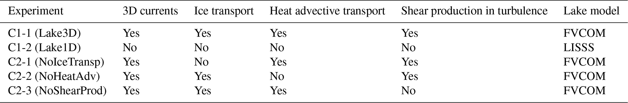
Case C2-1 (NoIceTransp) is designed to examine the impact of ice transport associated with currents (Sect. 5.1). In this scenario, FVCOM is configured identically to C1-1, except that ice dynamics, ice velocity fields, and ice pack transport are disabled in FVCOM. Instead, only ice thermal dynamics are simulated to account for the spatiotemporal evolution of ice thickness distribution through thermodynamic growth and melting processes (Bitz and Lipscomb, 1999). Consequently, the ice model is simplified to function as an energy-conserving thermodynamic model, akin to that used in the 1D lake model.

Case C2-2 (NoHeatAdv) analyzes the impact of 3D heat transport associated with lake circulation. FVCOM is configured identically to C1-1, except that the advective heat transport associated with current movement is disallowed in C2-2. This is realized by turning off the advection terms in the temperature equation in FVCOM, which is essentially an advection–diffusion equation that governs the distribution and evolution of temperature (Sect. 5.2). Therefore, the temperature calculation is simplified to imitate the 1D vertical diffusion equation used in the 1D lake model.

Case C2-3 (NoShearProd) aims to assess the influence of 3D currents on the calculation of turbulent mixing, a crucial factor in controlling the heat redistribution and thermal structure in the lakes. In this case, we exclude the turbulence shear production term that depends on currents in the turbulent kinetic equation (Sect. 5.3). In summary, the three cases in category 2 collectively reveal the significant impacts of currents on elements that are not accounted for in the LISSS 1D lake model, i.e., on ice transport, heat transport, and turbulent mixing intensity, respectively. These experiments are summarized in Table 1.

Table 1 A summary of the numerical model experiments. The “3D currents” column shows whether the experiment resolves the 3D currents of the Great Lakes. The “Ice transport” column shows whether the experiment resolves the ice transport associated with currents in the Great Lakes. The “Heat advective transport” column shows whether the experiment resolves the 3D heat transport associated with Great Lakes circulation. The “Shear production in turbulence” column shows whether the experiment uses the turbulence shear production term that depends on currents in the turbulent kinetic equation. The “Lake model” column shows the lake model used in the experiment.

4 Results

4.1 Evaluation of the NU-WRF/FVCOM performance

4.1.1 Lake temperature and ice cover

The NU-WRF/FVCOM (case C1-1) captures the seasonal evolution of LSTs well across all of the Great Lakes, with lake-mean LST root-mean-square errors (RMSEs) below 0.4 °C (Fig. 2a1–a5). In November, the lakes undergo rapid cooling, but the rate of the temperature decline varies by lake, primarily due to differences in depth and latitude. These factors contribute to pronounced spatial heterogeneity in LSTs across the lakes (Fig. 3a1–c1). While the model successfully reproduces the overall seasonal evolution, it misses some episodic fluctuations. For example, observational data from GLSEA show short-term spikes in both temperature and ice cover – such as the notable low-temperature and ice cover spikes in Lake Ontario during February – that are not fully captured in the simulation. The modeled LST and ice cover time series tend to appear smoother than those of the observations (Fig. 2a4 and b4). The GLSEA data and the 3D lake model align closely in terms of the spatial LST patterns, with warmer waters of 10–12 °C in the central and eastern basins of Lake Erie and Lake Ontario and 8–10 °C in the southern basins of Lake Michigan and Lake Huron, while much cooler temperatures are found across Lake Superior, ranging between 4 and 6 °C (Fig. 3). The most notable underestimation of LST by the 3D lake simulation occurs in the southern basin of Lake Huron, while the model captures the LSTs in the northern basin of Lake Huron. Also, the spatial pattern in the GLSEA observational data appears more heterogeneous on a finer scale compared to the 3D lake simulation. Transitioning to January 2015 (Fig. 3a2–c2) at the onset of the ice season, NU-WRF/FVCOM reflects the seasonal cooling of the lakes well, showing a significant reduction in LSTs while also delineating the detailed temperature differences between the colder nearshore and relatively warmer offshore waters well, in good agreement with the observational data. On the other hand, NU-WRF/LISSS (case C1-2) fails to capture the spatial heterogeneity in LSTs but also generates a systematic cold bias of 2–3 °C during January across nearly all of the lakes (Fig. 3c1–c2; Fig. S1 in the Supplement). Such a cold bias was persistent in the NU-WRF/LISSS (Lake1D) simulation throughout the cold season, as detailed in Notaro et al. (2021; Figs. 12 and 13).

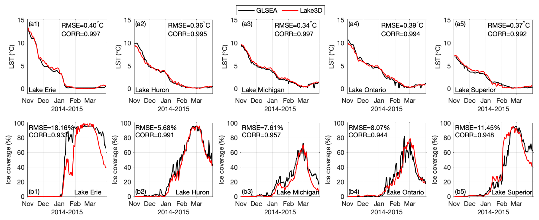
Figure 2 Time series of the daily lake-averaged LST (°C, a1–a5) and percent ice cover (b1–b5) for the five lakes from the GLSEA data (black lines) and NU-WRF/FVCOM 3D lake model simulations (red lines) during the simulation period of November 2014–March 2015. Both the temporal correlation and RMSE are reported in each panel.

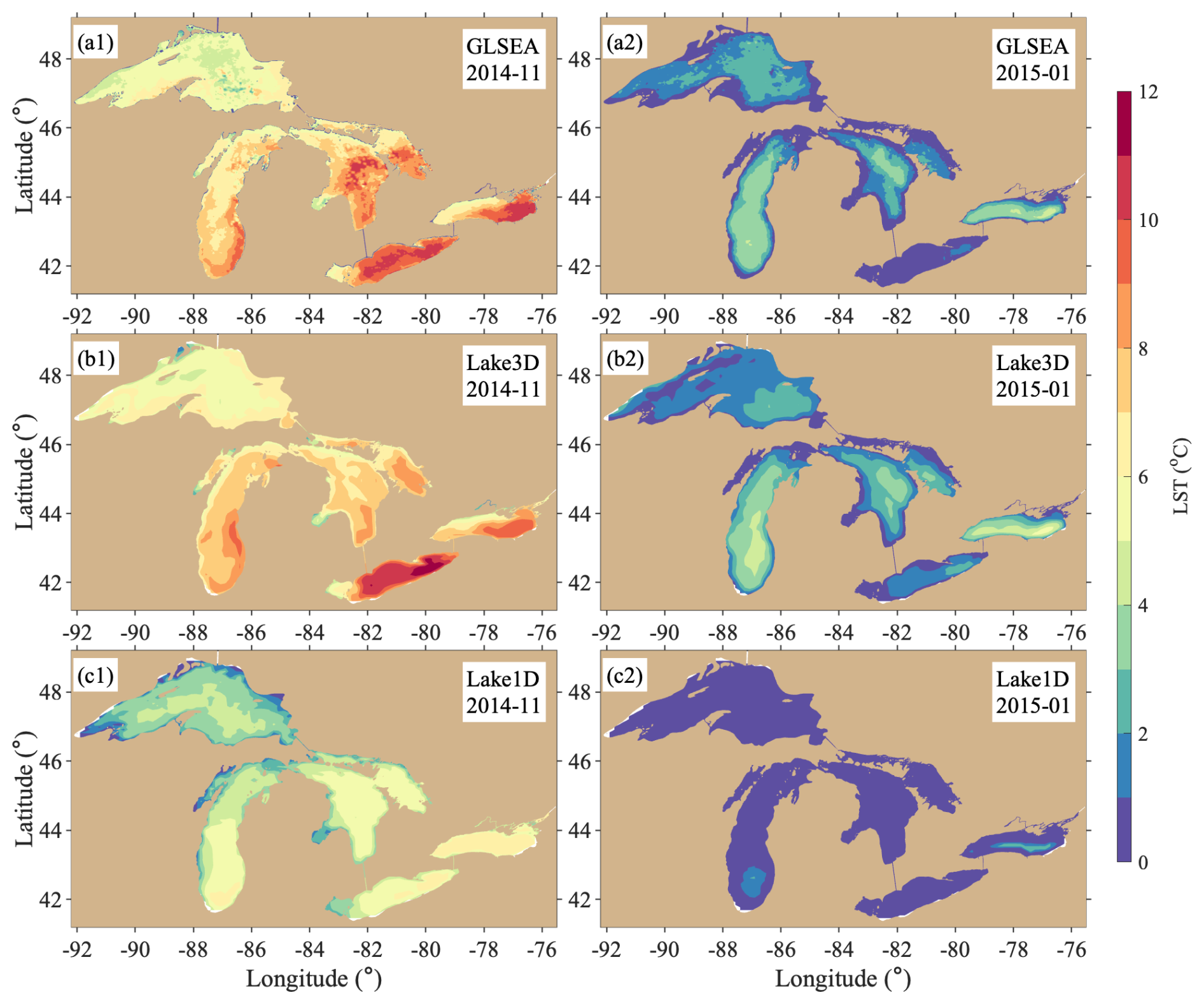
Figure 3 Spatial patterns of monthly mean LSTs (°C) from the GLSEA data (a1, a2), NU-WRF/FVCOM 3D lake model simulations (b1, b2), and NU-WRF/LISSS 1D lake model simulations (c1, c2) for November 2014 (left panels; a1–c1) and January 2015 (right panels; a2–c2).

NU-WRF/FVCOM (Lake3D) also demonstrates its skill in capturing the evolution of the vertical thermal structure within the lake, which is particularly challenging in large and deep lakes (Bennington et al., 2014; Xue et al., 2017). As exemplified in Fig. 4, the in situ thermistor measurement at the deep and central Lake Huron is located in a deep region with a water depth of 220 m. The 3D model reproduces the conclusion of the summer stratification process until the end of November. The following turnover, a seasonal process where the surface water cools, becomes denser, and sinks – mixing with the warmer water from below – are also represented in the 3D lake model between December and January. Subsequently, the winter inverse stratification, where colder water (<4 °C) lies above warmer water due to the fact that the freshwater's density peaks at 4 °C, is captured by the 3D model as it develops from February onward, although the model shows a stronger winter inverse stratification and earlier onset than observed. In contrast, NU-WRF/LISSS falls short of these detailed observations. Not only does it mispredict the occurrence of turnover and winter stratification much earlier than observed, it also substantially underestimates the extent of mixing between the surface and deeper waters. This underestimation results in a flawed representation of excessive surface cooling and a substantial overestimation of the warming of the deep waters.

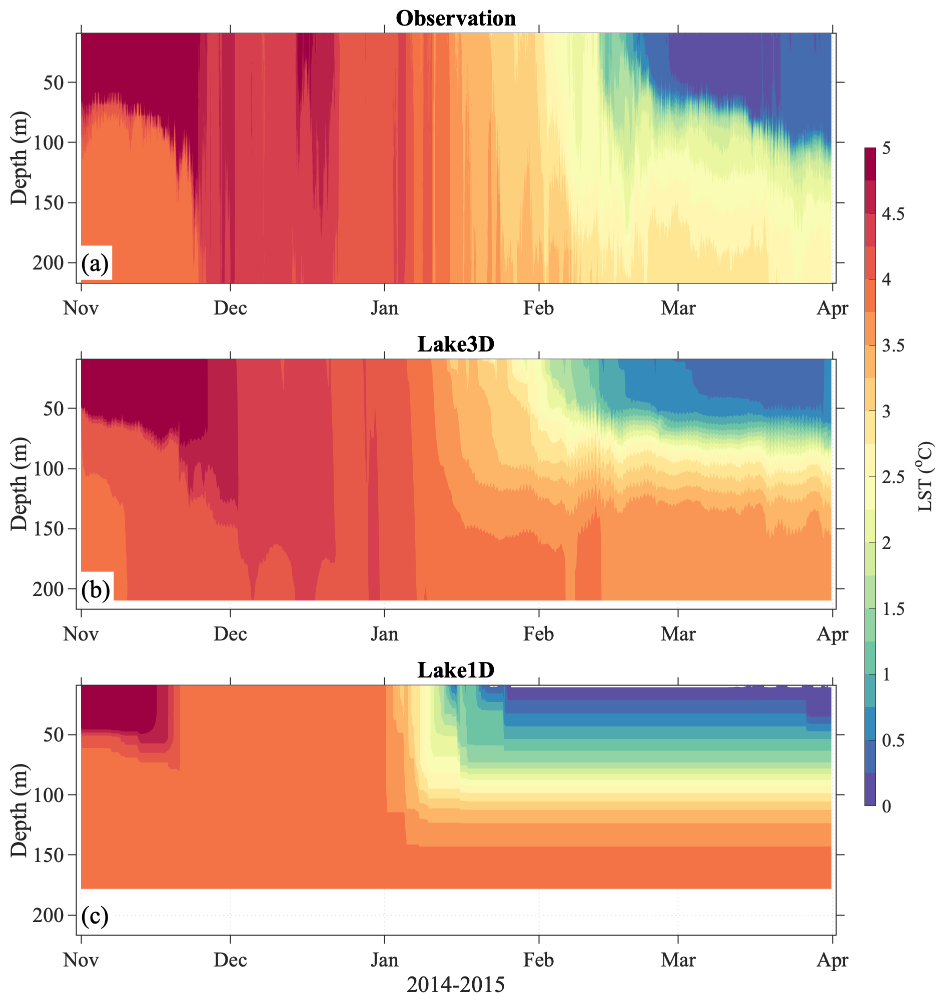
Figure 4 Seasonal evolution of daily vertical temperature (°C) profiles from the thermistor observations (a), the NU-WRF/FVCOM 3D lake model (b), and the NU-WRF/LISSS 1D lake model (c) at the central Lake Huron during November 2014–March 2015. The observation location is shown in Fig. 1.

Correspondingly, NU-WRF/FVCOM resolves the spatiotemporal evolution of lake ice cover very well across all of the lakes, with RMSE values of percent ice cover of less than 8 % for Lake Huron, Lake Michigan, and Lake Ontario and 11 % and 18 % for Lake Superior and Lake Erie (Fig. 2a2–e2). The 3D lake model and GLSEA data exhibit similar seasonal trends in both timing and magnitude, with ice cover typically starting to rapidly increase in January, peaking in February and early March, and declining thereafter. Lake Erie shows the earliest and sharpest increase in ice cover, peaking near 100 % in early February and throughout mid-March, which is indicative of its shallower depth and weaker thermal inertia. Lake Huron and Lake Superior show a persistent increase in ice cover through February, with the peak coverage of >90 % occurring at the beginning of March. Lake Michigan and Lake Ontario exhibit more gradual increases and lower peaks in ice cover. The model appears to capture the general seasonal trends of the GLSEA data with high fidelity, although some discrepancies are evident, particularly over Lake Erie and Lake Superior (Fig. 2b1–b5).

NU-WRF/FVCOM performs reasonably well in mirroring the general spatial patterns of lake ice cover (Figs. 5a1–a3 and b1–b3). For January, the GLSEA data show a pronounced ice formation in the nearshore regions across the lakes, with the greatest ice concentration visible along the coastlines and with very limited ice cover in offshore waters. The model captures this nearshore ice development quite well, although it suggests less ice cover in the offshore areas, particularly over Lake Erie. In February, the extent of the ice cover varies dramatically across the lakes, including nearly full ice cover on Lake Erie and significant ice-free areas on Lake Ontario, as well as Lake Michigan and Lake Huron, which have distinctly less ice cover in their southern and central basins, respectively. The model captures this variability very well while slightly overestimating the ice cover in the central regions of Lake Superior. For March, the model successfully replicates the patterns of significant declines in ice cover in the western sections of the lakes, with much higher ice coverage in the eastern sections of the lakes.

On the other hand, NU-WRF/LISSS (Lake1D) generates excessive ice cover during January (Fig. 5c1), when both observations and NU-WRF/FVCOM suggested that the majority of the lakes were ice-free (Fig. 5a1, b1). In February, the excessive ice cover simulated by the NU-WRF/LISSS model persists, with near-complete ice coverage over all of the lakes, and the model fails to depict the large spatial variability across the lakes (Fig. 5c2). Such a persistent overestimation of ice cover throughout the cold season by NU-WRF/LISSS was reported in Notaro et al. (2021; Fig. 13) and our Supplement (Fig. S1).

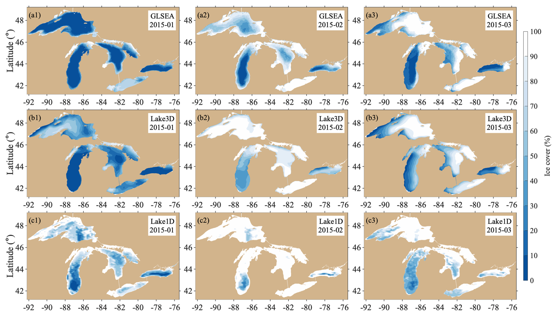
Figure 5 Spatial patterns of mean percent lake ice cover from GLSEA data (top panels; a1–a3), NU-WRF/FVCOM 3D lake model simulations (middle panels; b1–b3), and NU-WRF/LISSS 1D lake model simulations (bottom panels; c1–c3) for January, February, and March 2015.

4.1.2 Over-lake latent and sensible heat fluxes

The improved LST and ice simulation by the 3D lake model translates into an improvement in the simulated over-lake latent and sensible heat fluxes, particularly for the ice cover season (Fig. 6). The observations for upward latent and sensible heat fluxes from two eddy covariance flux towers at Granite Island on Lake Superior and Spectacle Reef on Lake Huron are compared with the simulated fluxes from NU-WRF/FVCOM (Lake3D) and NU-WRF/LISSS (Lake1D). Lake Superior and Lake Huron were selected for demonstration because studies have shown that the deeper, larger Great Lakes present more complex hydrodynamic challenges that 1D models consistently fail to represent accurately, often resulting in substantial errors. NU-WRF/LISSS reasonably simulates the magnitude and variability of the heat fluxes from November to mid-December, similar to the observations and NU-WRF/FVCOM, although with larger biases. However, it grossly underestimates the fluxes during the ice cover season (January–March) by simulating a nearly constant near-zero flux. This is mainly due to the excessive ice cover simulated by the 1D lake model, which creates a physical barrier for air–lake energy fluxes. Since the 3D lake model more accurately simulates the LST and ice cover, it successfully captures the magnitude and variability of the heat fluxes, even during the ice cover season, with RMSEs that are 50 % lower than those from the 1D lake model (Fig. 6).

Latent heat in Spectacle Reef is the only exception, where NU-WRF/FVCOM struggles to capture the magnitude of the upward latent heat flux due to the overestimated ice cover at the site (Fig. S2). Ice cover plays a critical role in modulating latent heat exchange: in the bulk aerodynamic formulation, latent heat flux is scaled by the open-water fraction, as ice acts as a physical barrier to evaporation and moisture transfer. A higher modeled ice fraction reduces the effective evaporation area, resulting in suppressed moisture exchange and, consequently, underestimation of latent heat flux. As shown in Fig. S2, the model substantially overestimates ice cover at this site in January and maintains a high ice concentration through February. This persistent overestimation directly reduces the open-water fraction, contributing to low latent heat. Interestingly, the observed latent heat flux remains elevated in February despite the observed ice cover approaching 90 %. This apparent discrepancy suggests potential uncertainty in either the observed ice cover, the latent heat flux measurements, or both, and it warrants further investigation.

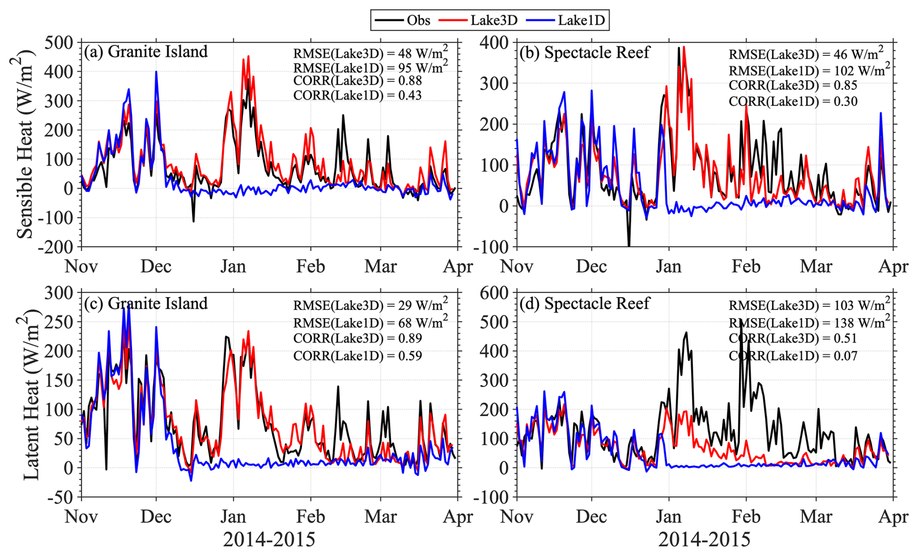
Figure 6 Time series of daily sensible (upper panels; a, b) and latent (lower panels; c, b) heat fluxes (W m⁻²) from GLEN observations (black lines), NU-WRF/FVCOM 3D lake model simulations (red lines), and NU-WRF/LISSS 1D lake model simulations (blue lines) at Granite Island on Lake Superior (a, c) and Spectacle Reef on Lake Huron (b, d). The RMSE and temporal correlations between the simulations and GLEN observations are provided in each panel.

4.1.3 Over-lake air temperature and wind

Along with the improved simulation of the Great Lakes' physical characteristics and surface heat fluxes, NU-WRF/FVCOM improves the simulated over-lake atmospheric state across the Great Lakes, including air temperature and wind speed. The cold air temperature biases produced over the lakes by NU-WRF/LISSS are significantly reduced (Fig. 7), with better-simulated, more intense upward heat fluxes in January. This improvement in the simulated air temperature at the two sites, Granite Island and Spectacle Reef, is evident. Similar to the fluxes, NU-WRF/LISSS-modeled air temperature diverges from the observations in January and February, with a noticeable cold bias. This cold bias is the result of significant suppression of the upward heat fluxes during these months in the 1D lake model due to excessive simulated ice cover. NU-WRF/FVCOM, on the other hand, produces a much warmer and more accurate over-lake air temperature for January and February due to its reasonable representation of upward heat fluxes. The simulated wind speed over the lakes is also improved, especially in January–February (Fig. 7). This advancement is attributed to the refined simulation of surface roughness (i.e., ice versus water), the water–air temperature gradient, and the associated instability over the lakes due to decreased ice cover. Large wind spikes (16 m s⁻¹) in January–February are better captured by NU-WRF/FVCOM. In addition, the two models' biases relative to observations are directly compared in Fig. S3.

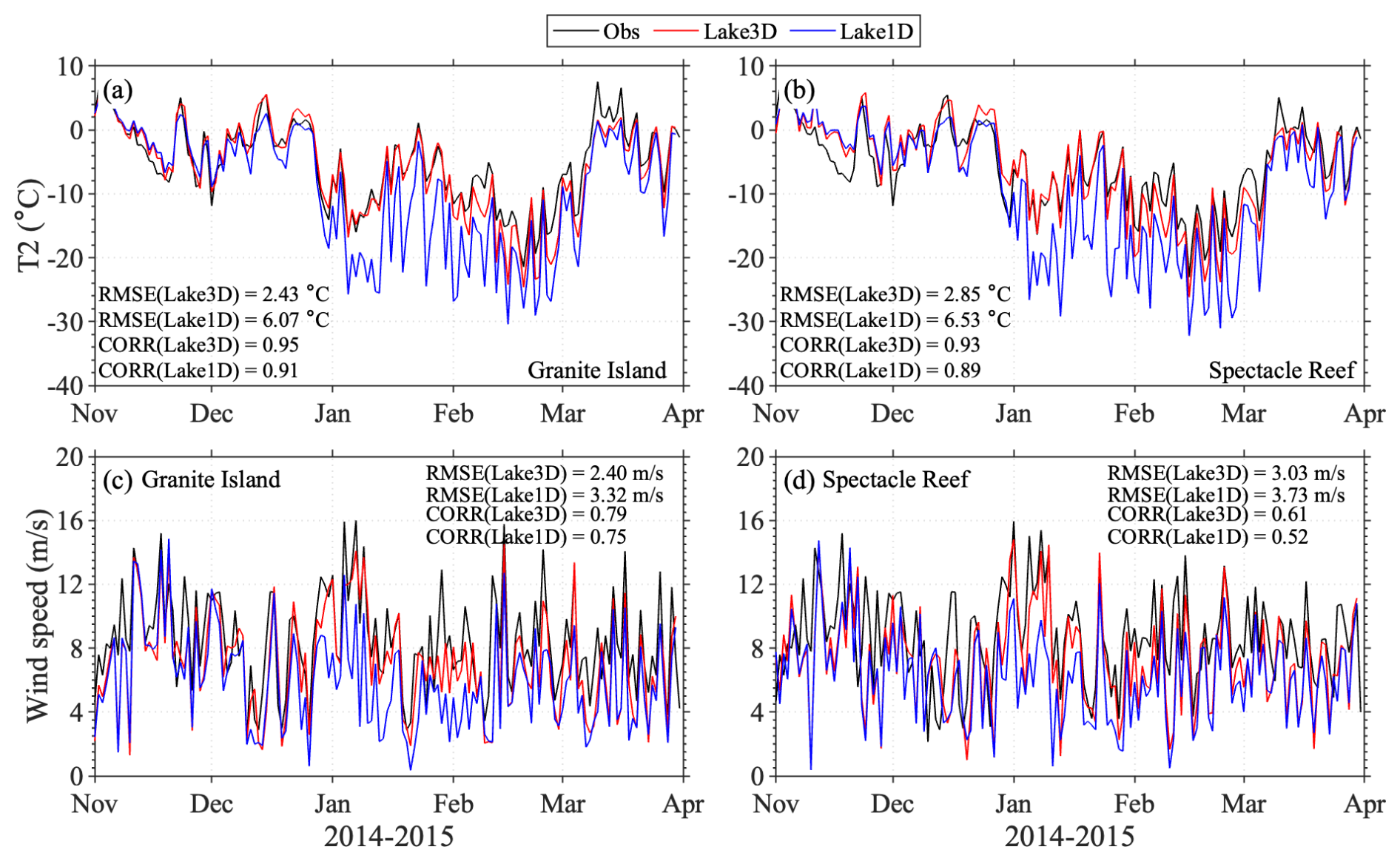
Figure 7 Time series of daily air temperature (°C, upper panels; a, b) at 2 m height (T2) and wind speed (m s⁻¹, lower panels; c, d) from GLEN observations (black lines), NU-WRF/FVCOM 3D lake model simulations (red lines), and NU-WRF/LISSS 1D lake model simulations (blue lines) at Granite Island on Lake Superior and Spectacle Reef on Lake Huron during November 2014–March 2015. The RMSE and temporal correlations between the simulations and GLEN observations are provided in each panel.

4.2 Diagnosing key hydrodynamic processes missing in 1D lake models

The Great Lakes modeling community has agreed on the pressing need to integrate 3D lake models instead of conventional 1D lake models in Great Lakes regional climate studies (Delaney and Milner, 2019). However, no studies have yet detailed the key 3D hydrodynamic processes that explain the superiority of 3D lake models to 1D lake models, especially regarding cold season performance. The primary goal of this study is to identify the key processes influencing lake thermal structure and ice cover that are missed by 1D lake models but captured effectively by 3D lake models, through a series of process-oriented experiments presented below. Note that, in the discussion of the C2 experiments below, the analyses are focused on the major 3D lake processes that influence the simulated limnological patterns of lake temperature and ice cover, not the overlying atmospheric conditions, which are beyond the scope of this study.

4.2.1 Impact of ice movement

Case C2-1 (NoIceTransp) is designed to examine the impact of ice transport on LSTs and the overlying atmospheric conditions compared to the standard case C1-1 (Lake3D). In case C2-1, ice dynamics, velocity fields, and ice pack transport are disabled in FVCOM. Instead, only ice thermal dynamics are simulated, as in the 1D lake model. Figure 8 compares cases C1-1 (Lake3D) and C2-1 (NoIceTransp), illustrating their performance in simulating the observed spatial pattern of ice coverage in March 2015 that is characterized by open water on the western side of the Great Lakes and predominant ice cover on the eastern side (Fig. 8a). Utilizing a 3D lake model that only accounts for ice thermal dynamics results in an overestimation of ice cover, with near-complete lake-wide ice cover in Lake Superior, Lake Huron, and Lake Erie (Fig. 8b). However, integrating ice dynamics, including transport influenced by wind and water–ice stress, results in excellent agreement with observations, highlighting the critical role of ice transport in ice modeling (Fig. 8c). This pattern aligns with the modeled ice velocities, which attribute the eastward ice cover distribution to dominant eastward ice transport (Fig. 8d). Under cold winter conditions characterized by strong westerly winds, ice is driven eastward, maintaining open water in the lake's western part. This facilitates ongoing atmospheric interactions, allowing for heat release. Neglecting these dynamics leads to unrealistic ice accumulation by diminishing the influence of wind on surface water movement and mixing. This overaccumulation of ice cover hampers the efficiency of vertical turbulent mixing, which is essential for maintaining a warmer surface layer, thereby exacerbating ice formation and accumulation. The incorporation of ice dynamics into 3D lake models is thus essential for simulating ice distribution, emphasizing the necessity of resolving ice transport to accurately replicate observed patterns.

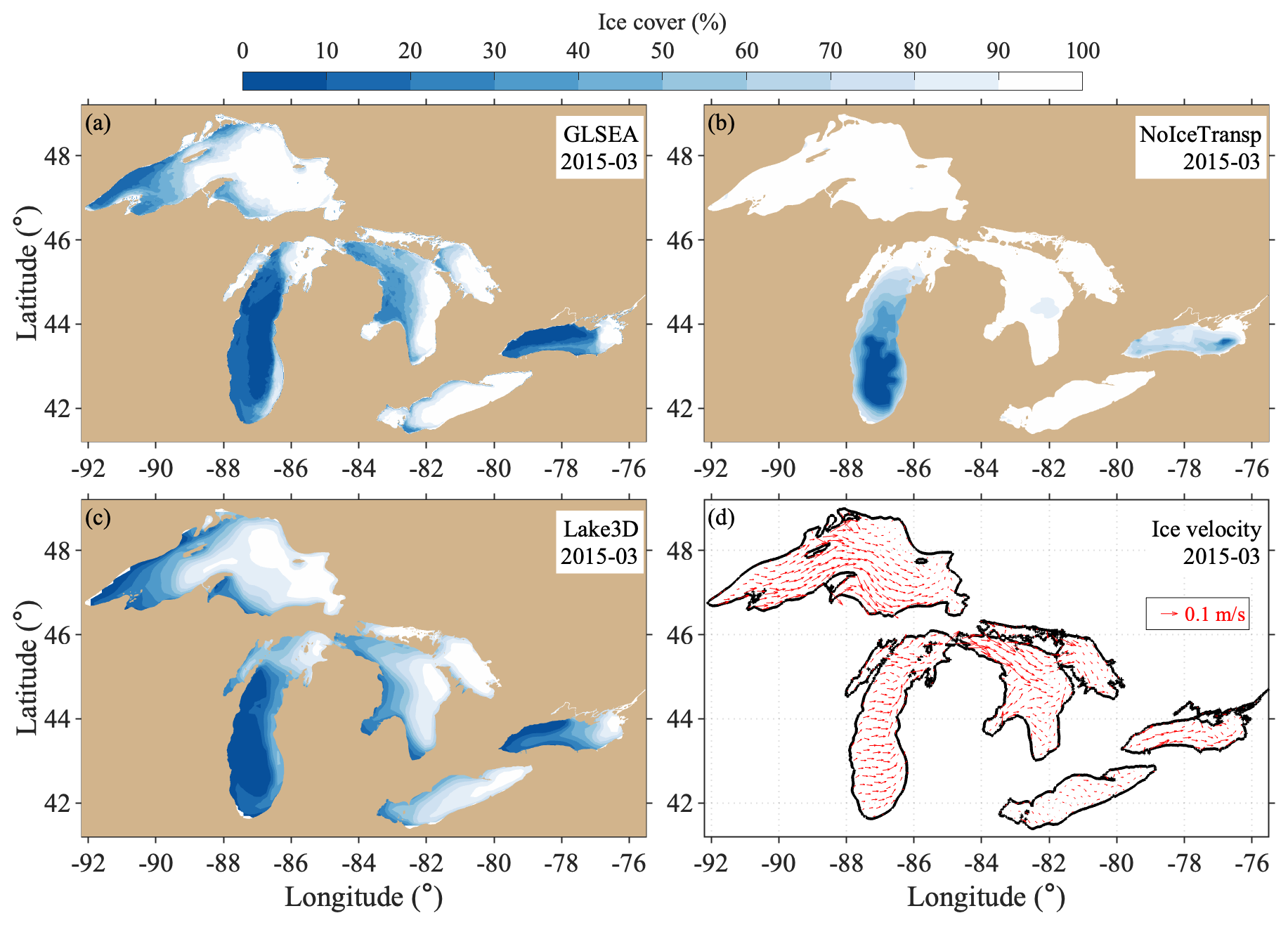
Figure 8 Spatial patterns of mean percent lake ice cover from GLSEA data (a), case 2-1 (NoIceTransp) simulations (b), and case 1-1 (Lake3D) standard simulations (c), along with simulated mean ice velocities (m s⁻¹) during (d) March 2015.

4.2.2 Impact of advective heat transport

The next set of simulations focuses on the impact of within-lake heat transport. As discussed previously, the 3D lake model resolves the advective transport of heat associated with the simulated circulation. Case C2-2 (NoHeatAdv) analyzes the impact of 3D heat transport. In this case, the 3D temperature advection terms ($u\frac{\partial T}{\partial x}v\frac{\partial T}{\partial y}w\frac{\partial T}{\partial z})$ from Eq. (1) are turned off.

Comparing the standard simulation C1-1 (Lake3D) to case C2-2 (NoHeatAdv), Fig. 9 demonstrates that, in the absence of advective heat transport by lake currents, the surface temperatures can remain consistent with the basic patterns observed in the standard 3D lake simulation throughout the entire simulation period. The differences in the time series of lake-wide average LSTs for the five lakes are small, with a maximum difference of 0.4 °C between the two cases. The spatial patterns of LST biases, when compared with GLSEA, are generally more noticeable, with the most significant positive biases (∼ 2 °C) concentrated around the coastal waters of the Great Lakes and eastern Lake Erie from January to March 2015 and larger negative biases (∼ 3 °C) in the central basin of Lake Huron in November 2014 in the NoHeatAdv case.

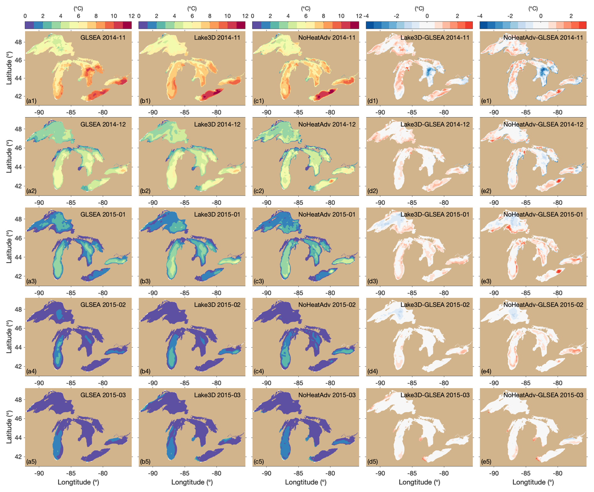
Figure 9 Spatial patterns of mean LSTs (°C) from GLSEA data (a1–a5), case C1-1 (Lake3D) standard simulations (b1–b5), and case C2-2 (NoHeatAdv) simulations (c1–c5) from November 2014 to March 2015. Their monthly biases relative to GLSEA data are presented in panels (d1)–(d5) and (e1)–(e5), respectively.

However, disabling heat advection significantly affects the lake's thermal structure, as shown for the in situ thermistor measurement at the deep, central Lake Huron, which is located in a deep region with a water depth greater than 200 m. Case C2-2 (NoHeatAdv) generally reproduced the thermal patterns from case C1-1 (Lake3D) in terms of both the timing and intensity of summer stratification, fall turnover, and winter inverse stratification (Fig. 10a, c). While the comparison shows that the overall thermal structures are similar in both simulations, there is a noticeable difference within the subsurface layer, specifically between depths of 50 and 80 m (Fig. 10d), suggesting that heat advection might have a more significant impact on temperature distribution in the subsurface layer of the water column in this case. Without accounting for heat advective transport, there appear to be artifacts of stepwise vertical thermal gradients in case C2-2 (Fig. 10c). For readers interested in side-by-side comparisons of thermal structure differences across different model cases (e.g., Lake3D, Lake1D, Lake3D without ice transport, and Lake3D without shear-induced mixing), the results are compiled in Fig. S4.

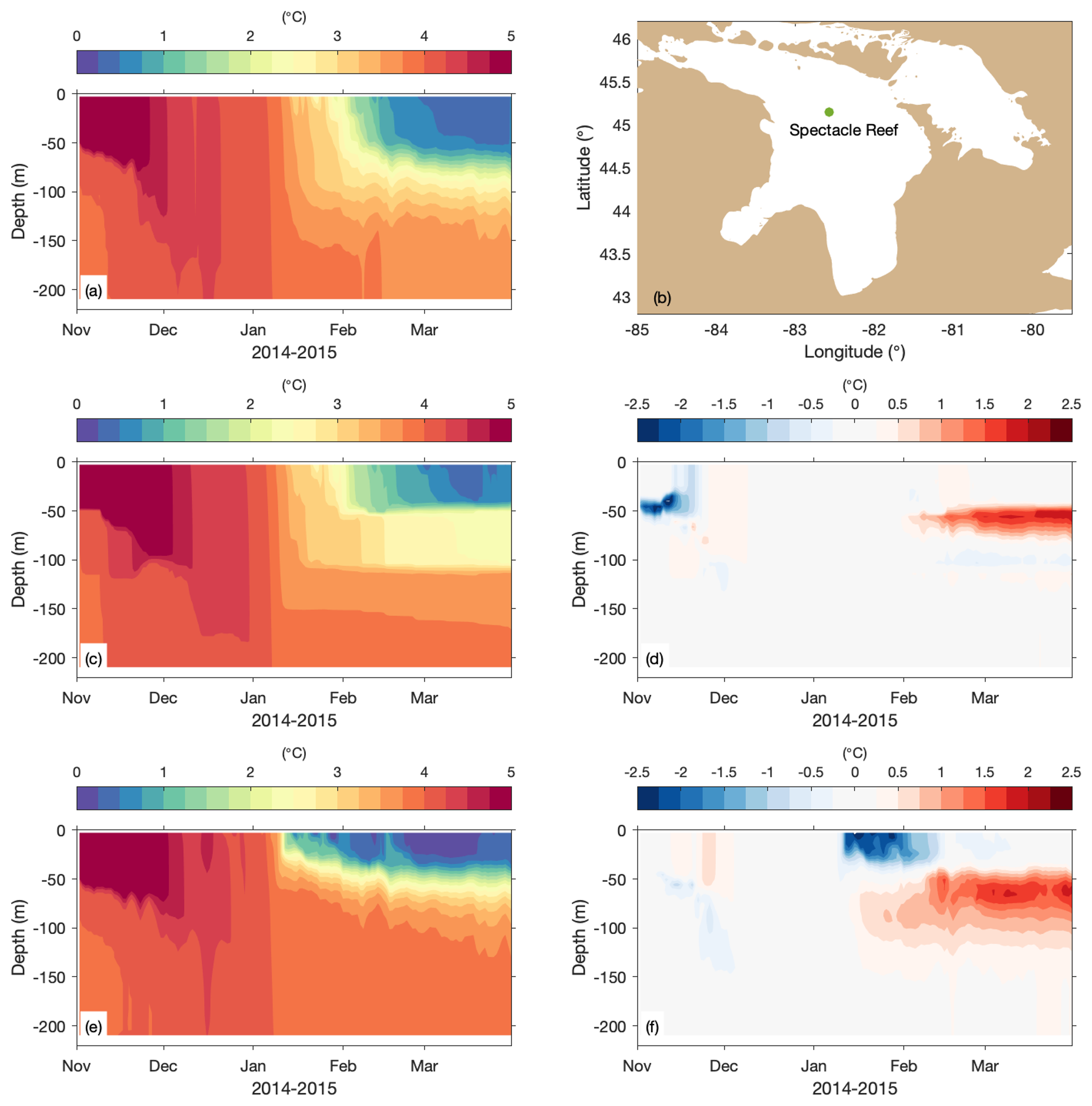
Figure 10 Mean vertical temperature (°C) profiles at central Lake Huron from (a) the case C1-1 (Lake3D) standard run and (b) the thermistor observation site. (c) Case C2-2 (NoHeatAdv) and (d) its difference relative to case C1-1. (e) Case C2-3 (NoShearProd) and (f) its difference relative to case C1-1. Note that the results shown in panels (e) and (f) are discussed in the following section on the impact of vertical mixing.

To gain a deeper understanding of the results, we analyzed the heat balance to identify the contributions of different physical processes. This analysis involved examining each term in the temperature-governing equation (Eq. 1) that is directly computed in FVCOM over the simulation period. The temperature change is driven by 3D advective heat transport, horizontal heat diffusion, and vertical diffusion due to turbulent mixing.

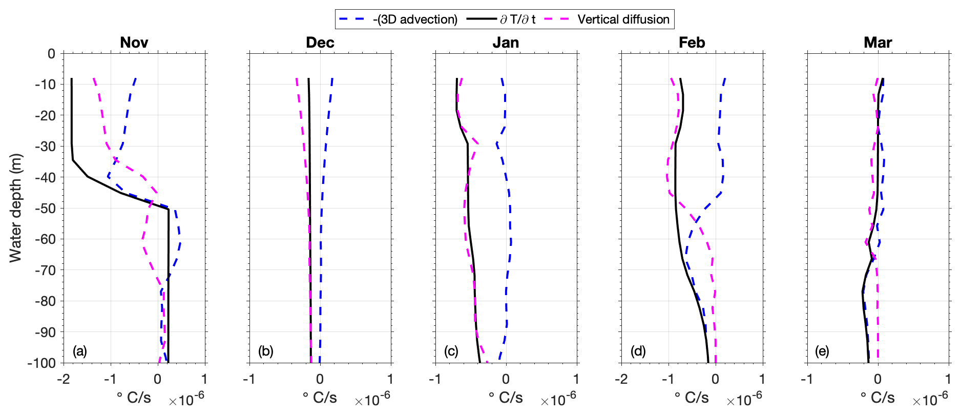
Figure 11 Monthly averaged vertical profiles of key terms in the temperature equation in the C1-1 (Lake3D) simulation at the deep-water thermistor site (220 m) in central Lake Huron (the site location is in Fig. 1) from November 2014 through March 2015. The black line represents the temperature change rate ($\partial T/\partial t$), while the dashed blue and magenta lines represent the contributions from 3D advection and vertical diffusion, respectively. Horizontal diffusion is omitted here due to its negligible contribution throughout the winter season.

Figure 11 illustrates the monthly averaged vertical profiles of key terms in the temperature equation from the Lake3D (C1-1) simulation at the deep-water thermistor site in central Lake Huron. The figure is used to identify the dominant physical processes driving temperature change at various depths during the cold season. Figure 11 shows that vertical turbulent mixing – represented by the vertical diffusion term – is a major contributor throughout the season, particularly in December and January. During these 2 months, it dominates temperature change throughout the upper 100 m due to strong mixing (as also indicated in Fig. 10a). However, 3D advection also plays a critical role, particularly near the surface (upper 40 m) in November and at intermediate depths (60–80 m) in February and March, where the temperature change rate ($\partial T/\partial t$) closely aligns with the advection term (Fig. 11a, d, e). The growing importance of advection in these months is reinforced by Fig. 10c, which shows that disabling the advection term results in the largest temperature biases at the subsurface (40 m) in November and at 60–80 m in February and March. In contrast, minimal impact is shown in December and January, when temperature changes are primarily governed by vertical mixing. Together, these results underscore the need to resolve both vertical turbulent mixing and 3D advective processes to simulate winter thermal dynamics in large, deep lakes.

4.2.3 Impact of vertical mixing

The analysis above (Fig. 11) highlights the dominant factor, vertical turbulent mixing, in determining seasonal lake temperature change. Note that we have already discussed the importance of ice transport associated with currents as well as the impact of advective heat transport. To understand the mechanism responsible for the differing performance between the 1D and 3D lake models in simulating vertical mixing, now, we examine how vertical turbulent mixing is calculated in these two types of models.

Figure 12 reveals that, in the Great Lakes, shear production – induced by the vertical gradient of horizontal velocity in the water column – is the primary driver of subsurface turbulent mixing, i.e., the dominant source term balancing the dissipation rate (sink term), while the other terms – buoyancy production and 3D advection of turbulent kinetic energy (TKE) – play a secondary role, being at least 1 order of magnitude smaller than shear production in the first 60 m of depth. This underscores the importance of including the current simulation when estimating the vertical turbulent mixing, which is crucial for simulating heat exchange in the water column and ultimately determining the lake's thermal structure and ice formation.

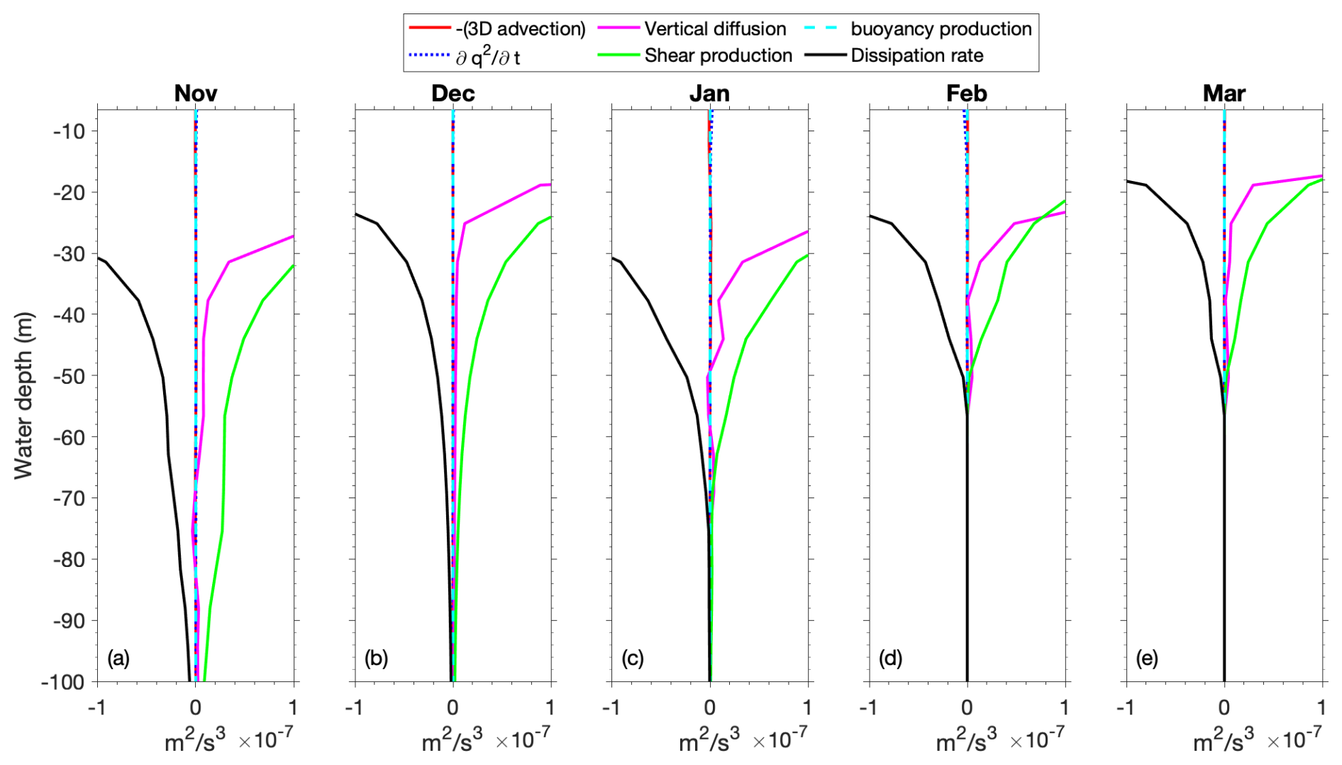
Figure 12 Monthly averaged vertical profile of each term of the turbulence kinetic equation in the C1-1 (Lake3D) simulation at the deep-water thermistor site (220 m) in central Lake Huron (the site location is in Fig. 1) from November 2014 through March 2015. The profiles include shear production (green), buoyancy production (dashed cyan), vertical diffusion of TKE (magenta), dissipation rate (black), 3D advection of TKE (dashed red), and the TKE change rate term $\partial q^{\mathrm{2}}/\partial t$ (dotted blue). Shear production is the dominant source term balancing the dissipation rate (sink), while the other terms – buoyancy production and 3D advection – are comparatively smaller in magnitude. The dominance of shear-driven mixing emphasizes the importance of resolving realistic current structures.

Correspondingly, Fig. 10a, e, f compare the vertical temperature profiles between the standard simulation C1-1 (Lake3D) and case C2-3 (NoShearProd). The NoShearProd case shows stronger stratification, particularly from January to March. The absence of shear production leads to significantly reduced turbulent mixing and limited heat exchange between surface and deeper waters, which results in a colder surface layer (0–40 m) and warmer deep waters (50–120 m) compared to the standard run (Fig. 10f). Consequently, the colder surface water temperature favors ice formation, leading to overestimated ice cover in the NoShearProd case compared to the standard simulation and observations, particularly in January and February (Fig. 13). For readers interested in side-by-side comparisons of ice cover across different model cases (e.g., NU-WRF/FVCOM, NU-WRF/LISSS, Lake3D without ice transport, and Lake3D without shear-induced mixing), the results are compiled in Fig. S5.

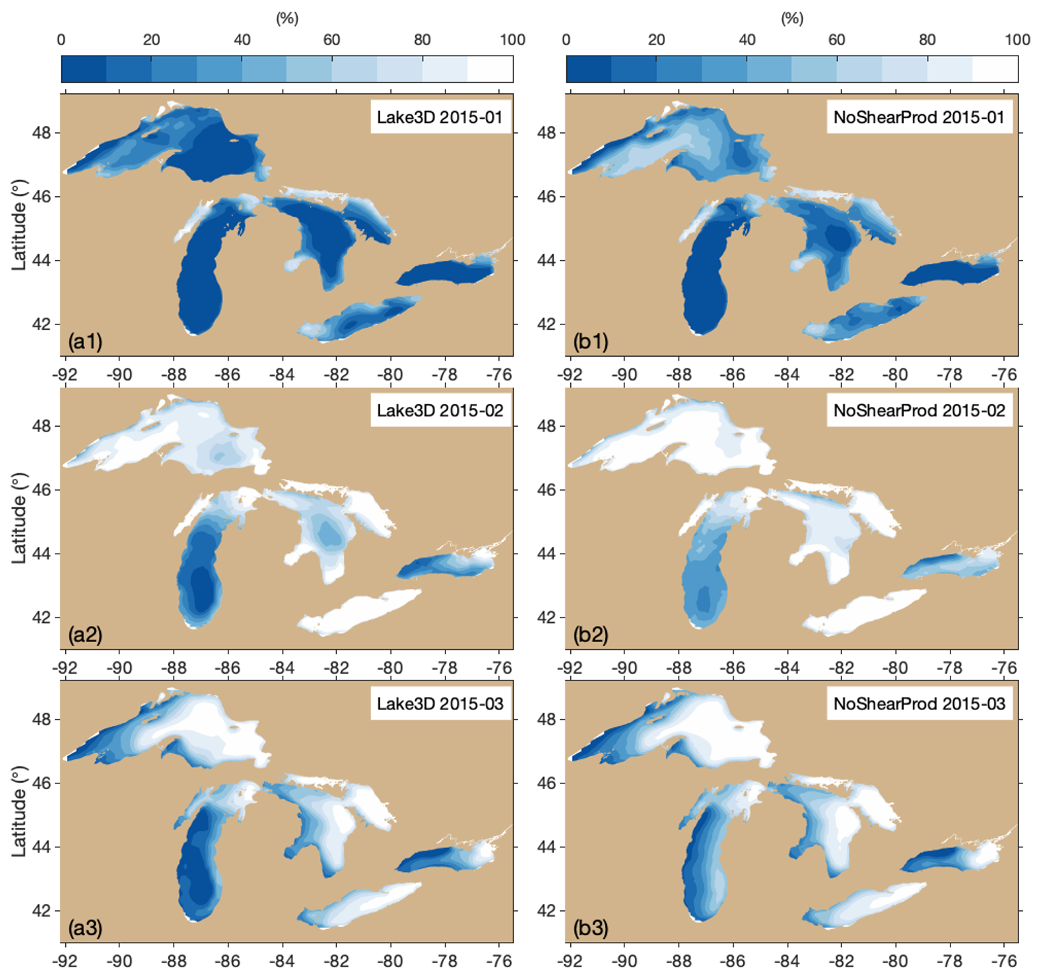
Figure 13 Spatial patterns of mean percentage lake ice cover from case C1-1 (Lake3D; a1–a3) and case C2-3 (NoShearProd; b1–b3) for January, February, and March 2015.

5 Discussion

We systematically identify three key hydrodynamic processes that are absent in 1D lake models but resolved in 3D models, which accounts for the improved cold season performance in simulating LST and ice cover: (1) lateral ice transport, (2) advective heat transport, and (3) shear-induced turbulence. Critically, all three of these processes are dynamically linked to water currents – spatially and temporally evolving flow fields that are fundamentally unresolved or crudely simplified in 1D lake models. This represents the key scientific insight of our study: these dominant hydrodynamic processes responsible for realistic wintertime lake thermal structure and ice cover are current-driven and are thus structurally absent in 1D models. This finding constitutes the key contribution of our work and, we believe, offers an important step forward in understanding why 3D models perform better – not merely that they do.

While 1D column lake models have been widely used in the simulations of inland lakes worldwide, small inland lakes and the Great Lakes exhibit fundamental differences in their physical characteristics, such as size and depth, which in turn influence their mixing behaviors, thermal structures, and circulation patterns. Inland lakes, which are generally much smaller (with a typical average area of 1–10 km) and much shallower (with a typical average depth of ∼ 10 m), respond more rapidly to atmospheric conditions. This leads to a fairly uniform horizontal pattern and a simpler mixing process in response to surface wind due to their shallow depth and small thermal inertia. Therefore, 1D column lake models serve as appropriate and efficient tools for simulating inland lake processes, particularly when the lake depth is shallower than 20 m. In contrast, the vast size (e.g., Lake Superior alone covers about 82 100 km²) and significant depth (e.g., the average depth of Lake Superior is 147 m, with a maximum depth of 400 m) of the Great Lakes result in complex hydrodynamic and thermal dynamics. This complexity causes the Great Lakes to exhibit many sea-like characteristics that require 3D hydrodynamic modeling to resolve.

LISSS, as is true of other 1D lake models, was originally designed for small and shallow inland lakes and was not designed to resolve water currents (Subin et al., 2012; Notaro et al., 2021). Some other 1D lake models (Stepanenko and Lykossov, 2005; Stepanenko et al., 2011) employ a crude representation of average flow fields. Therefore, 1D lake models rely on empirical or semi-empirical relationships to estimate how wind stress affects the lake's turbulence and mixing without explicitly resolving 3D velocity fields. These thermal diffusion-based models often employ a latitude-dependent Ekman decay, accompanied by an empirical modification factor, to estimate a lumped eddy diffusivity coefficient as an approximation for surface-wind-induced mixing (Subin et al., 2012; Xiao et al., 2016). Thus, the lack of accurate simulation of turbulent mixing processes makes the 1D model of limited use in simulating the Great Lakes' thermal structure.

We emphasize that this study is not driven by an effort to improve 1D lake models or to refine 3D lake models further. Rather, our focus is on understanding the fundamental hydrodynamic processes absent in 1D models and how they are resolved in 3D frameworks. That said, we acknowledge that both 1D and 3D lake modeling approaches offer opportunities for improvement. For instance, 3D lake models in the Great Lakes region still face challenges in accurately reproducing thermal structure, such as underestimating stratification strength or mixed-layer depth (Ye et al., 2020). Conversely, previous studies have shown that 1D lake models can be tuned to better match observations (e.g., via lumped eddy diffusivity; Xiao et al., 2016; Bennington et al., 2014). However, such tuning improves historical performance without addressing the lack of mechanistic representation of key physical processes.

This limitation becomes particularly critical when models are used for future climate projections under nonstationary conditions. Empirical or simplified physical relationships calibrated to present-day conditions may not hold under altered forcing scenarios, introducing significant uncertainty. While tuning may be effective when extensive validation data are available, its reliability diminishes when applied to future climate conditions. Therefore, we advocate for the full integration of physically based 3D hydrodynamic lake models in a two-way-coupled framework for climate projection applications. This approach ensures that projections are grounded in physical processes, thereby improving robustness and reducing the risk associated with empirical parameterizations.

Within this context, the core contribution of this research lies in advancing our understanding of central questions in Great Lakes regional climate modeling: what are the key hydrodynamic processes missing from 1D lake models – processes that are critical for simulating lake thermal structure and ice cover during the cold season – and how are these processes resolved in 3D lake models? Our findings provide generalized insights that are not dependent on specific model configurations, tuning strategies, or the reproduction of individual observed events, making them broadly applicable across different modeling systems and lake conditions.

6 Summary and conclusion

In summary, the two-way-coupled NU-WRF/FVCOM (CLIAv1) has been developed for the next generation of a regional climate model for the Great Lakes Basin for accurate representations of lake–ice–atmosphere interactions. NU-WRF/FVCOM significantly improved on the performance of NU-WRF coupled with an optimized 1D lake model and more accurately reproduced the physical characteristics of the Great Lakes (e.g., LST, ice cover, and thermal structure). This led to further improvements in simulated over-lake atmospheric conditions (e.g., air temperature, wind, and latent and sensible heat) through two-way lake–atmosphere interactions.

This study has highlighted key hydrodynamic processes that differentiate the large, deep Great Lakes from small, shallow inland lakes and how these processes impact lake simulations. Specifically, we identified that ice dynamics, particularly ice transport, are vital in the Great Lakes, influencing ice cover formation and heat exchange between the lakes and the atmosphere. Secondly, we show that advective heat transport, which facilitates both lateral and vertical redistribution, enables a more realistic simulation of the complex spatial temperature patterns, particularly the predominance of advective heat transport in the subsurface layers. Thirdly, we identified the critical role of resolving shear production in turbulent mixing in the Great Lakes, which is the most influential factor that determines heat transfer and, subsequently, lake thermal structure. Ice transport, heat transfer, and shear production in turbulence mixing are fundamentally linked to the 3D lake currents, which are missing or crudely represented in 1D lake models. Our findings underscore that circulation currents are pivotal in the winter limnology of the Great Lakes. Given the ongoing impact of climate change on these aquatic systems (Zhong et al., 2016; Woolway et al., 2021; Cannon et al., 2024), incorporating 3D lake dynamics becomes crucial for projecting future thermal structures and ecosystem effects.