Optimized step size control within the Rosenbrock solvers for stiff chemical ordinary differential equation systems in KPP version 2.2.3_rs4

Numerical integration of multiphase chemical kinetics in atmospheric models is challenging. The underlying system of ordinary differential equations (ODEs) is stiff and thus difficult to solve. Rosenbrock solvers are a popular choice for such tasks. These solvers provide the desired stability and accuracy of results at an affordable yet large computational cost. The latter is crucially dependent on the efficiency of the step size control. Our analysis indicates that the local error, which is the key factor for the step size selection, is often overestimated, leading to very small substeps. In this study, we optimized the first-order step size controller most commonly employed in Rosenbrock solvers. Furthermore, we compared its efficiency to a second-order step size controller. We assessed the performance of the controllers in both a box and a global model for very stiff ODEs. Significant reductions in the computation time were accomplished with only marginal deviations in the results compared to the standard first-order controller. This was achieved not only for gas-phase chemistry but also for the more complex aqueous-phase chemistry in cloud droplets and deliquescent aerosols. Depending on the selected chemical mechanism, significant improvements were already achieved by simply adjusting heuristic parameters of the default controller. However, especially for the global model, the best results were achieved with the second-order controller, which reduced the number of function evaluations by 43 %, 27 % and 13 % for gas-phase, cloud and aerosol chemistry, respectively. The overall computational time was reduced by over 11 % while requiring only minimal adjustments to the original code. Analysis of a 1-year integration period showed that with the second-order controller, the deviations from the reference simulation stay below 1 % for the main tropospheric oxidants. The results presented here show the possibility of more efficient atmospheric chemistry simulations without compromising accuracy.

1 Introduction

Atmospheric chemistry modeling plays an essential part in understanding and predicting air composition and its interactions within the Earth's system. The chemical kinetics used in these models can be very complex (e.g., Rosanka et al., 2021a; Pozzer et al., 2022) and rely on the numerical solution of stiff systems of ordinary differential equations (ODEs), normally responsible for the largest part of the computing time (Christou et al., 2016). The systems of ODEs can be written as

$$\begin{array}{}\text{(1)}& {\mathit{y}}^{\prime }=P(t,\mathit{y})-L(t,\mathit{y}),\end{array}$$

where y is the array of concentrations (in cm⁻³); y^′ is the derivative of y with respect to time t; and P(t,y) and L(t,y) are the production and loss terms of the species, respectively. For stiff ODEs, implicit solvers with adaptive time stepping are preferably used (Sandu et al., 1997b). Stiffness refers to a situation in which an explicit ODE solver needs a time step that is “too small”, resulting in too many discretization steps to approximate the solution at the desired precision. However, a more objective definition of stiffness exists, and a criterion for identifying a problem as stiff has been defined by Spijker (1996):

$$\begin{array}{}\text{(2)}& \max Re\left({\mathit{\lambda }}_j\right)<\mathrm{0},{\displaystyle \frac{\max \left|Re\right({\mathit{\lambda }}_j\left)\right|}{\min \left|Re\right({\mathit{\lambda }}_j\left)\right|}}\mathit{>>}\mathrm{1},\end{array}$$

where Re(λ_j) values are the real parts of the eigenvalues of the Jacobian matrix, J(t,y), associated with the ODE system from Eq. (1). Atmospheric chemical kinetic models satisfy this criterion because the mechanisms always contain very fast and very slow reactions that occur on drastically different timescales (Sandu et al., 1997b). In a typical operator splitting framework, chemical kinetics has to be solved every few minutes after many non-chemical processes, e.g., emissions, which perturb the chemical composition. Thus, numerical integrators are not efficient because at every starting point, for a model time step of 10–20 min, they require very short initial substeps (10⁻⁵ s or shorter). In chemical kinetic terms, this is generally related to the perturbation of the chemical environment (long-lived species) that determines the concentrations of short-lived species. In mathematical terms, stiffness is related to the large negative values of λ_j that are associated with the diagonal elements of the Jacobian matrix (J_jj(t,y)). The latter are usually related to the loss term L_j(t,y) and thus to the lifetime of the species j (Turanyi et al., 1993). However, this is not the case for multiphase chemical mechanisms, for which large negative values of λ_j cannot always be associated with a single short-lived species but rather with fast acid-base equilibria or phase-transfer reactions (Sandu et al., 1997b). The ODE systems describing chemical kinetics in deliquescent aerosols with low liquid water content (LWC) and extremely fast outgassing of dissolved species are particularly stiff. This has strongly limited the ability to perform multiphase chemistry simulations with explicit kinetics (Kerkweg et al., 2007). Only recently has it become possible to perform numerical integration of chemical kinetics in deliquescent aerosols throughout the troposphere in a global model for LWC as low as 10⁻¹⁴ m³(aq) m⁻³(air) (Rosanka et al., 2024). However, such simulations pose a large burden on the computational resources needed and limit the understanding of the role of multiphase chemistry in atmospheric composition. Thus, there is a need for more efficient ODE integrators. Many numerical integrators are available and have been used for atmospheric applications (Zhang et al., 2011). At the maximal error that is usually accepted (1 %), Rosenbrock methods have proven to be the most efficient among the implicit solvers that offer the required stability for stiff problems (Sandu et al., 1997a). Linearly implicit Rosenbrock methods are a popular choice for solving such stiff ODE systems because of their suiting stability while not relying on costly solutions of nonlinear equations (Zhang et al., 2011). However, the precision and efficiency of these discretization methods depend on the control strategy used to adaptively adjust the integration step size. Ways of making these integrators more efficient have involved, for instance, manual or semi-automatic reduction of the ODE system size (Sander et al., 2019; Wiser et al., 2023; Lin et al., 2023). What is less explored are the improvements in efficiency by using a more sophisticated step size control. The adaptive time step controller that is usually employed in many applications, including chemical solvers, controls the locally produced error r_i to be within a tolerable threshold ε. The asymptotic behavior of the numerical solver is used to adaptively approximate the largest possible step size that is within the tolerance. The resulting step size controller

$$\begin{array}{}\text{(3)}& h_{i+\mathrm{1}}=h_i\sqrt[k]{{\displaystyle \frac{\mathit{\epsilon }}{r_i}}}\end{array}$$

was introduced by Hairer et al. (1993), where h_i is the time step size for the ith step and k is usually the order of convergence of the solver plus 1 ($k=p+\mathrm{1}$). Here, ε is a predefined relative error tolerance, and r_i is the local error produced by the solver's solution y_i compared to the real solution y at the corresponding point in time t_i. Chemical solvers usually make use of low values of p (Shampine and Witt, 1995; Sandu et al., 1997b). Additionally, Rosenbrock solvers, as part of the Runge–Kutta solver family, offer an efficient approximation of the local error with the help of a second embedded solver, which yields a second solution $\widehat{y}$ of lower order $\widehat{p}$ with nearly no extra effort (Hairer et al., 1993). This approximation is denoted as ${\mathit{l}}_i={\mathit{y}}_i-{\widehat{\mathit{y}}}_i$ from now on and is a substitute for the exact local error r_i. In practice, this controller is extended with some heuristic measures to ensure stability. Equation (4) shows the heuristic extensions and represents the controller we investigate in this work:

$$\begin{array}{}\text{(4)}& h_{i+\mathrm{1}}=h_i\cdot \min \left(q_{\max },\max \left(q_{\min },\mathit{\delta }\sqrt[\widehat{p}+\mathrm{1}]{{\displaystyle \frac{\mathrm{1}}{\left|\right|l_i\left|\right|}}}\right)\right).\end{array}$$

The new step size is multiplied by a safety factor δ, and the step size growth is limited with an upper and a lower value, called q_min and q_max, respectively. This practice was also proposed by Hairer et al. (1993) and also deemed appropriate for Rosenbrock solvers in Hairer and Wanner (1996). Nevertheless, a small difference to the implementation we use is that ε in the numerator is replaced by 1 because the tolerance is incorporated into the local error norm $\left|\right|{\mathit{l}}_i\left|\right|$. Equation (5) shows the implemented error norm $\left|\right|{\mathit{l}}_i\left|\right|$, which is similar to the scaled Euclidean norm from Hairer et al. (1993). There y_i,j is the jth component of the solver solution for the ith time step, and ${\widehat{\mathit{y}}}_{i,j}$ is the corresponding solution of the embedded, lower-order integrator. The scaling factor of the difference contains the absolute and relative tolerances, ε_abs and ε_rel, which have to be specified by the user. This normalizes the error, which means that steps are accepted if the error norm is equal to or less than 1. In the context of atmospheric chemistry, rather large tolerances as high as ${\mathit{\epsilon }}_{\mathrm{rel}}={\mathrm{10}}^{-\mathrm{2}}$ and ${\mathit{\epsilon }}_{\mathrm{abs}}=\mathrm{100}{\mathrm{cm}}^{-\mathrm{3}}$ are used (Zhang et al., 2011) because other uncertainties in Earth system models are considered to be larger.

$$\begin{array}{}\text{(5)}& \left|\right|{\mathit{l}}_i\left|\right|=\sqrt{{\displaystyle \frac{\mathrm{1}}{n}}\sum _{j=\mathrm{1}}^n{\left({\displaystyle \frac{{\mathit{y}}_{i,j}-{\widehat{\mathit{y}}}_{i,j}}{{\mathit{\epsilon }}_{\mathrm{abs}}+{\mathit{\epsilon }}_{\mathrm{rel}}\cdot max\left(\right|{\mathit{y}}_{i-\mathrm{1},j}|,|{\mathit{y}}_{i,j}\left|\right)}}\right)}^{\mathrm{2}}}\end{array}$$

However, Söderlind (2003) developed a suite of time step controllers based on control theory aspects. This idea is practicable because the aspired relative tolerance given by the user can be interpreted as a target value and the local error in each step as the actual value that the controller needs to adjust by reacting to the behavior of the ODE system. Many of these controllers are of a higher order of adaptivity than the first-order controller presented in Eq. (4). One of the second-order controllers is the H211b:

$$\begin{array}{}\text{(6)}& h_{i+\mathrm{1}}=h_i{\left({\displaystyle \frac{\mathit{\epsilon }}{\left|\right|{\mathit{l}}_i\left|\right|}}\right)}^{\mathrm{1}/(b\cdot k)}{\left({\displaystyle \frac{\mathit{\epsilon }}{\left|\right|{\mathit{l}}_{i-\mathrm{1}}\left|\right|}}\right)}^{\mathrm{1}/(b\cdot k)}{\left({\displaystyle \frac{h_i}{h_{i-\mathrm{1}}}}\right)}^{-\mathrm{1}/b},\end{array}$$

with b and k being free parameters of the controller. The parameter k is the root exponent that is already known from the currently used controller, where it was set to $\widehat{p}+\mathrm{1}$. This means that one could set $k=\widehat{p}+\mathrm{1}$. However, Söderlind (2003) suggests that this selection is in no way predetermined. To be more precise, the value should not be lower than $\frac{\widehat{p}+\mathrm{1}}{\mathrm{2}}$ and not too large; $\widehat{p}+\mathrm{1}$ is just a value that always produces a converging step size control (Deuflhard and Bornemann, 2008). The second parameter should be b>1 for stability, with increasing values creating a smoother and more robust step size sequence.

In this article, we improve the step size control implemented in the Rosenbrock solvers available with the Kinetic Pre-Processor (KPP) version 2.2.3 (Sandu et al., 1997a; Sandu and Sander, 2006). The KPP software is mainly used to solve the very stiff sets of ODEs resulting from the kinetics of atmospheric chemical mechanisms of varying complexity in the gas phase (e.g., Pozzer et al., 2022), in cloud droplets (e.g., Rosanka et al., 2021a) and deliquescent aerosols (Rosanka et al., 2024). In brief, KPP translates input files containing chemical reactions and rate constants into source code files containing the resulting ODE system, as well as an integrator chosen by the user. KPP is frequently applied in atmospheric models across multiple scales, ranging from simple box models (e.g., Chemistry As A Boxmodel Application (CAABA) by Sander et al., 2019) to complex regional and global atmospheric chemistry models (e.g., ECHAM/MESSy Atmospheric Chemistry (EMAC) by Jöckel et al., 2010). We first evaluate the step size control within the CAABA box model. Based on the results, we present adjustments to the first-order controller and compare its performance to the second-order step size controller H211b presented by Söderlind (2003). To evaluate our adjustments under varying atmospheric conditions, we also performed global simulations with EMAC.

2 Methodology

2.1 Chemical kinetic model

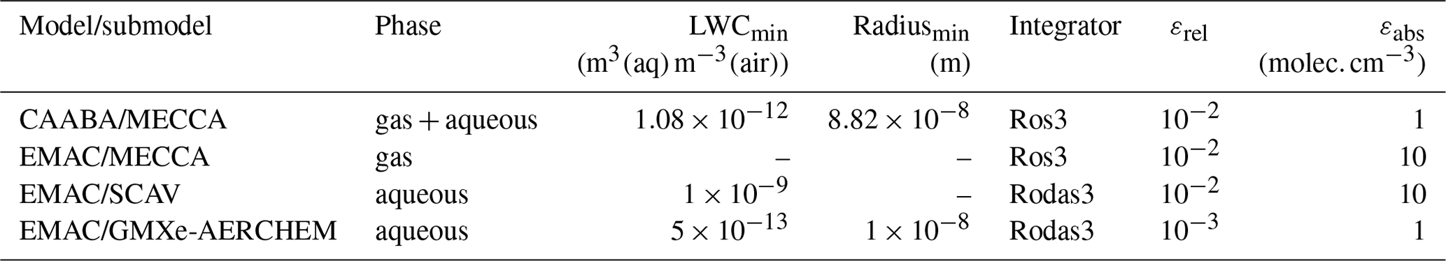
Multiphase chemistry is represented by the kinetic model in the Module Efficiently Calculating the Chemistry of the Atmosphere (MECCA) (Sander et al., 2019). The rate of phase-transfer reactions is governed by the liquid water content (LWC), water solubility and the mass-transfer coefficient according to Kerkweg et al. (2007) following the formulation by Sander (1999). The inorganic gas-phase chemistry mainly follows the recommendations by JPL (Burkholder and et al., 2019) and IUPAC (Wallington et al., 2018). The organic gas-phase chemistry in MECCA is represented by the Mainz Organic Mechanism (MOM), which includes organics up to C₁₀ molecules for isoprene (Taraborrelli et al., 2012; Nölscher et al., 2014; Novelli et al., 2020), monoterpenes (Hens et al., 2014; Mallik et al., 2018) and aromatics (Cabrera-Perez et al., 2016; Taraborrelli et al., 2021). In total, MOM represents 735 chemical species and 2196 reactions. The inorganic aqueous-phase chemistry is represented by a comprehensive set of reactions for species containing oxygen, nitrogen, sulfur and halogens (Kerkweg et al., 2008). The aqueous-phase chemistry of organics up to C₄ molecules is represented by the Jülich Aqueous-phase Mechanism of Organic Chemistry (JAMOC; Rosanka et al., 2021b). JAMOC represents 792 chemical species and 1148 reactions (Rosanka et al., 2021b).

2.2 Box model

We used the community box model Chemistry As A Boxmodel Application (CAABA) in this study (Sander et al., 2019). It represents chemical and physical (emission, dry deposition, entrainment, photolysis) processes in the atmosphere in a simplified manner. CAABA is coupled to the submodel MECCA, which contains a comprehensive set of multiphase chemical reactions. Based on these, KPP creates one large system of ODEs for the gas phase and two condensed phases, representing populations of deliquescent aerosols (LWC = $\mathrm{1.08}\times {\mathrm{10}}^{-\mathrm{12}}$ m³(aq) m⁻³(air), $r=\mathrm{8.82}{\mathrm{10}}^{-\mathrm{8}}$m) and cloud droplets (LWC = $\mathrm{3.04}\times {\mathrm{10}}^{-\mathrm{11}}$ m³(aq) m⁻³(air), $r=\mathrm{1.67}{\mathrm{10}}^{-\mathrm{6}}$ m). The Rosenbrock integrator used is Ros3 with relative and absolute tolerances of ${\mathit{\epsilon }}_{\mathrm{rel}}={\mathrm{10}}^{-\mathrm{2}}$ and ${\mathit{\epsilon }}_{\mathrm{abs}}=\mathrm{1}{\mathrm{cm}}^{-\mathrm{3}}$, respectively. We have defined three scenarios which emphasize different parts of the chemical mechanism by changing initial concentrations and emissions:

1. The marine boundary layer (marine). Gas-phase chemistry interacts with aqueous-phase chemistry in marine aerosol particles. The initial concentrations and emissions are based on Vogt et al. (1996) with modifications available in CAABA for the MBL case.

2. A coastal megacity (megacity). Anthropogenic emissions of hydrocarbons interact with halogen- and sulfur-containing compounds from the sea. The initial concentrations and emissions are taken from Crippa et al. (2018) and Huang et al. (2015).

3. A pristine tropical rain forest (forest). Biogenic isoprene and terpenes are emitted into the air and then oxidized in a complex degradation scheme. The initial concentrations are taken from Table 2 in Taraborrelli et al. (2009).

Table 1 Overview of the (sub)models used and the corresponding specifications of the chemistry and integrator for the performed simulations.

2.3 Global model

The ECHAM/MESSy Atmospheric Chemistry (EMAC) model is a numerical chemistry and climate simulation system that includes submodels describing tropospheric and middle-atmospheric processes and their interaction with oceans, land and human influences (Jöckel et al., 2010). It uses the second version of the Modular Earth Submodel System (MESSy2) to link multi-institutional computer codes. The core atmospheric model is the fifth-generation European Centre Hamburg general circulation model (ECHAM5; Roeckner et al., 2006). The physics subroutines of the original ECHAM code have been modularized and reimplemented as MESSy submodels and have continuously been further developed. Only the spectral transform core, the flux-form semi-Lagrangian large-scale advection scheme and the nudging routines for Newtonian relaxation remain from ECHAM. For the present study we applied EMAC (MESSy version 2.55.2) in the T42L31 resolution, i.e., with a spherical truncation of T42 (corresponding to a quadratic Gaussian grid of approx. 2.8 by 2.8° in latitude and longitude) and with 31 vertical hybrid pressure levels up to 10 hPa. The global model is run in a quasi-chemical transport mode (QCTM) without feedbacks between chemistry and physics (Deckert et al., 2011). This ensures that the meteorology of the model and its influence on tracer concentration remain identical in all the simulations performed. Therefore, any difference in tracer abundance is purely attributable to the different integration of the chemical ODE.

Like CAABA, EMAC uses MECCA to represent chemical kinetics. The same parameter space of the box model can be explored for testing in the global model. Unlike the box model and early EMAC simulations (Kerkweg et al., 2007), EMAC now relies on so-called operator splitting to represent chemistry in the gas phase and in deliquescent aerosols separately, in series (Rosanka et al., 2024, their Fig. 1a). In the simulations performed in this study, we use MECCA to represent gas-phase chemistry, including some heterogeneous reactions, whereas aqueous-phase chemistry in convective and large-scale clouds and rain is represented using the SCAvenging (SCAV) submodel (Tost et al., 2006). Aerosol processes are represented using MESSy's Global Modal-aerosol eXtension (GMXe; Pringle et al., 2010) submodel. Here, aqueous-phase chemistry in accumulation and coarse deliquescent aerosols is represented by the sub-submodel AERosol CHEMistry (AERCHEM; Rosanka et al., 2024), which is part of the GMXe submodel. AERCHEM is executed only when the liquid water content of the aerosols is larger than $\mathrm{5}\times {\mathrm{10}}^{-\mathrm{13}}$ m³(aq) m⁻³(air). From the available KPP Rosenbrock methods, we chose Ros3 for MECCA (gas phase) and Rodas3 for SCAV and GMXe-AERCHEM (aqueous phase) due to favorable performance and stability (Rosanka et al., 2024). For the tolerances, MECCA and SCAV both use ${\mathit{\epsilon }}_{\mathrm{rel}}={\mathrm{10}}^{-\mathrm{2}}$ and ${\mathit{\epsilon }}_{\mathrm{abs}}=\mathrm{10}{\mathrm{cm}}^{-\mathrm{3}}$. Due to higher stiffness and lower stability when solving aqueous-phase chemistry in deliquescent aerosols, AERCHEM uses a relative tolerance of ${\mathit{\epsilon }}_{\mathrm{rel}}={\mathrm{10}}^{-\mathrm{3}}$ and an absolute tolerance of ${\mathit{\epsilon }}_{\mathrm{abs}}=\mathrm{1}{\mathrm{cm}}^{-\mathrm{3}}$.

For all EMAC simulations performed in this study, biogenic emissions are represented by the Model of Emissions of Gases and Aerosols from Nature (MEGAN; Guenther et al., 2012). Biomass-burning-related emissions are calculated by MESSy's BIOBURN submodel, which combines biomass burning emission factors with dry-matter combustion rates obtained from the Global Fire Assimilation System (GFAS) based on Moderate Resolution Imaging Spectroradiometer (MODIS) satellite instruments (Kaiser et al., 2012). Sea-spray aerosol emissions are calculated online following the methodology by Kerkweg et al. (2006). We represent mineral dust as bulk inert dust; i.e., no crustal elements are emitted, with online emissions calculated following Astitha et al. (2012). All anthropogenic emissions follow the Emissions Database for Global Atmospheric Research (EDGAR v4.3.2; Crippa et al., 2018).

2.4 Simulations performed

Global model simulations are much more complex than box model ones, and more efficient simulations would save costly computation time on high-performance computing (HPC) systems, which offers the opportunity for longer simulation periods or more complex chemistry mechanisms. However, we started with CAABA box model simulations because their reduced complexity allows for an easier analysis of the step size selection and local error behavior of the step size controllers.

The box model simulations covered a simulation period of 12 h, and output was written at every model time step of 10 min. We also added output of the local error, step size and number of function evaluations for every integrator time step. All simulations were done for all three presented scenarios. Besides reference simulations with the default values of the first-order controller, we made simulations for every single parameter change, like an increased safety factor. To evaluate changes in precision, we also made another reference simulation with a fully implicit fifth-order Radau integrator and a relative tolerance of ${\mathit{\epsilon }}_{\mathrm{rel}}={\mathrm{10}}^{-\mathrm{7}}$ and absolute tolerance of ${\mathit{\epsilon }}_{\mathrm{abs}}=\mathrm{1}{\mathrm{cm}}^{-\mathrm{3}}$.

Given that global model simulations require much more computational effort, we reduced the number of values tested for each parameter, and the simulation period for the first set of simulations only covers the first day of the year 2009. MECCA, SCAV and AERCHEM produce a single ODE system each. Therefore, in each 1 d simulation we changed one parameter of one submodel. Output was produced after each model time step of 15 min. After exploring the influence of the different parameters, we also made 1-year simulations for the year 2009 with the best-performing parameters of the first-order controller and the second-order controller. For runtime and error comparisons, a reference 1-year simulation which contains the current default settings was made as well. To have an acceptable amount of I/O, we only wrote output every 23rd hour. With this selection we have output for every day of the year, and after 24 d there is output for each hour (0 to 23). The global simulations were done on the JUWELS cluster supercomputer from the research center in Jülich. We used eight nodes with 48 cores each.

3 Step size control in the box model

3.1 First-order controller

In this section, the efficiency of the standard first-order step size controller from Eq. (4) is assessed on the basis of the CAABA simulations for the three presented scenarios. Hereby, we focus on two key aspects: (1) the step size and (2) the local error. The specific KPP implementation of the controller and the error norm used are also described in Sandu et al. (1997a). Further, we provide the pseudocode of the implementation in Appendix A.

3.1.1 Evaluation

The local error estimation is quite crucial for an efficient solution because it is the main factor influencing the next step size. If the estimated value is too large, this could lead to an inefficient step size sequence with unnecessarily small step sizes. For this reason, we compared a more accurate approximation of the local error to the one calculated by the integrator. To obtain this precise estimation, we proceeded as follows:

1. step size h is calculated as usual;

2. the area $[t,t+h]$ is divided into five equally distant areas;

3. each of the five areas is viewed as its own local integration problem, starting at $t+\frac{j}{\mathrm{5}}h$ and ending at $t+\frac{j+\mathrm{1}}{\mathrm{5}}h$, $j\in \mathit{\{}\mathrm{0},\mathrm{1},\mathrm{2},\mathrm{3},\mathrm{4}\mathit{\}}$;

4. the local problems are solved one after another with the same solver and parameters used for the actual ODE;

5. the result of the fifth local problem is a precise approximation of the solution at position t+h;

6. instead of the embedded solution $\widehat{\mathit{y}}$, we can now use this solution to calculate a more precise local error norm $\left|\right|\mathit{l}\left|\right|$.

The division into five equally distant areas produces a solution with a precision of ${\mathit{\epsilon }}_{\mathrm{rel}}^{\mathrm{5}}$, which is sufficient for our investigations. This procedure obviously required much more computation time and is not practical in real applications but provides a very precise local error. For simplification, we refer to this estimation in the following as the real local error.

Exemplified by the marine scenario, Fig. 1 shows that the general course of the estimated local error is fairly good and closely follows the one of the real local error. However, it can be seen that the solver nearly always overestimates the local error for accepted steps. Furthermore, the error frequently becomes very small, sometimes going below 10⁻⁶, even though the border for acceptance is 1. Both of these findings show potential to increase the efficiency of the controller while staying within the desired tolerances. The overestimation leads to smaller step sizes than necessary for the majority of the steps, leading to many avoidable computations. This is because, by the definition of the controller in Eq. (4), $\left|\right|{\mathit{l}}_a\left|\right|>\left|\right|{\mathit{l}}_b\left|\right|$ implies h_a<h_b. In addition, in some cases the overestimation led to step rejections even though the real error would have been accepted; however, this happened in less than 5 % of the visualized 250 steps. Moreover, the regularly occurring local error dips indicate that there were areas where the selected step size was much smaller than necessary. Focusing on the local error dips, Fig. 2 illustrates that the decreases in the local error occurred in areas where the step size drastically increased after the step size dropped to a very small value. This indicates that the step size could grow faster in these areas than it does currently.

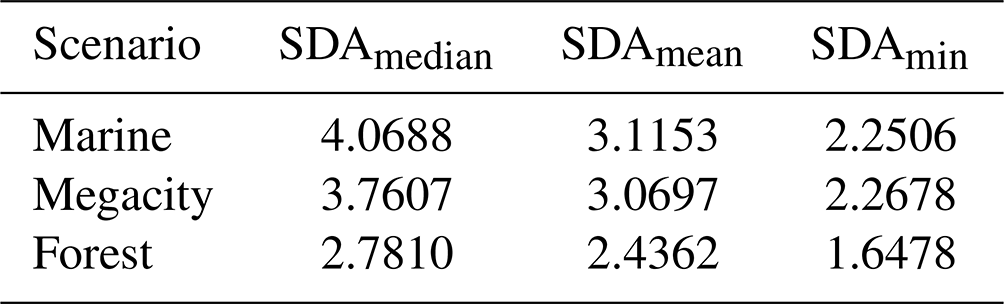
Generally, our findings indicate that a more aggressive strategy with higher step size selection could work to reduce the required computations while still being within the accepted error margin. To be able to verify this, we compared the simulations with changed parameters to the simulation with the Radau integrator. With these reference results, the number of significant digit places was calculated (see Appendix B). Evaluations of the precision of the standard first-order controller showed that the component-wise median number of significant digits for the marine scenario was as high as 4, instead of the aspired 2 (see Table B1). The average was also noticeably above the target of 1 %.

3.1.2 Optimization

The investigations from the previous section demonstrated that there is considerable potential to improve the step size selection to speed up the integration process without losing the aspired precision. This led to the idea of adjusting the step size controller to be more generous with the step size in some areas, considering the overestimation of the local error and its regular decreases to small orders of magnitude. The easiest way to adjust the behavior of the standard controller was with the heuristic parameters listed in Table 2. Most of the default values have already been suggested by Hairer et al. (1993) as universally valid options because they are more conservative and focus on stability. Our goal was to find values that suit the ODE systems of the tested mechanisms, yielding a lower numerical workload. Therefore, a range of appropriate values was tested for each parameter independently. As a measure of the computational effort of the integrator, the number of function evaluations was taken because it is independent of hardware and computations outside the ODE system, in contrast to other measures, e.g., the simulation runtime. Optimally, the number of computations should decrease without the single-digit accuracy (SDA) dropping below 2. SDA represents the number of significant digits.

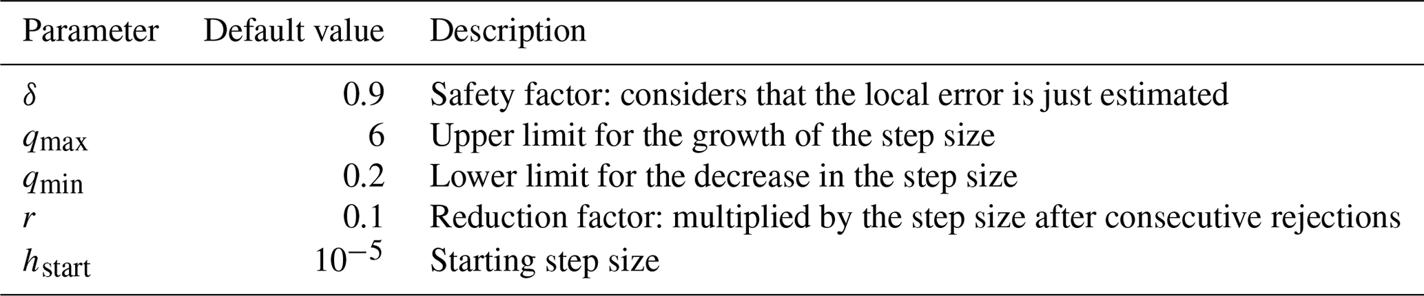
Table 2 Default heuristic parameters of the standard first-order controller as from KPP2 (Sandu and Sander, 2006).

The historically developed heuristic assumption of decreasing the step size with a safety factor (δ<1) for precautionary reasons is in contrast to the results of our local error analysis. Based on our analysis in Sect. 3.1.1, we now know the actual ratio between the estimated and the real local error. This made it possible to obtain a well-founded estimation of the safety factor. Equation (7) shows how we estimated the values used for this work.

$$\begin{array}{}\text{(7)}& \mathit{\delta }\sqrt[p+\mathrm{1}]{{\displaystyle \frac{\mathrm{1}}{\left|\right|\mathit{l}\left|\right|}}}\stackrel{!}{=}\sqrt[p+\mathrm{1}]{{\displaystyle \frac{\mathrm{1}}{\frac{\mathrm{1}}{V}\left|\right|\mathit{l}\left|\right|}}}\end{array}$$

The leftmost side of the equation shows the relevant part of the controller in Eq. (4). If we assume that the estimated local error is larger than the real local error by a factor of V, we can incorporate this factor into the controller equation by using $\frac{\mathrm{1}}{V}\left|\right|\mathit{l}\left|\right|$ as the denominator. By factoring V out of the root in Eq. (7), we get $\sqrt[p+\mathrm{1}]{V}$ as an estimation for a new safety factor.

$$\begin{array}{}\text{(8)}& \mathit{\delta }=\sqrt[p+\mathrm{1}]{V}\end{array}$$

This results in a safety factor of δ≈1.4, slightly varying for each CAABA scenario. Simulations with various values for $\mathit{\delta }\in [\mathrm{0.9},\mathrm{1.7}]$ showed that values near the calculated optimum led to a quite significant reduction in function evaluations without a meaningful decrease in precision, as shown in Fig. 3 for the megacity and marine scenarios. The figures display work–precision diagrams similarly to Sandu et al. (1997b). Instead of the CPU time, the number of function evaluations is plotted against the SDA of the least precise component with the largest relative error. Details on how SDA is calculated can be found in Appendix B. Overall, values in the range of $\mathit{\delta }\in [\mathrm{1.3},\mathrm{1.5}]$ seemed to be the most promising because they provide a significant reduction in function evaluations of up to 31 % while ensuring a smoother step size sequence than higher values. The most notable finding was that the first increases had a big impact on the reduction in work, but as the safety factor grew larger, its influence diminished.

The analysis of the local error led to the assumption that the step size may grow faster in certain situations to address the significant drops in the local error. Therefore, increasing the upper growth limit factor q_max appeared to be a fitting measure to reduce the numerical burden. Figure 4 seems to support this theory. It shows the calculated growth factor and the upper limit q_max that clips exceeding values. The results were taken from the marine scenario simulation. There seems to be a correlation between areas where the calculated growth factor exceeded q_max and areas where the local error became very small (compare Fig. 1). Model runs with q_max values between 6 and 30 were made, but the results showed that nearly no reduction in the number of function evaluations was achieved – the best was a reduction of 3 %, but in most cases it was much less. This was most likely the case because this increase only saved a few evaluations per peak. Considering that there were only four peaks within the first 250 steps, the benefit was small. The nearly constant overestimation of the local error seems to impact the efficiency of the solver more than the significant drops within the local error. The parameter q_max is not able to compensate for the nearly constant overestimation of the local error because it only influences a small part of the step sizes. Thus, parameters that have an impact on the majority of steps, like the safety factor, can achieve better improvements and indirectly reduce the decreases in the local error.

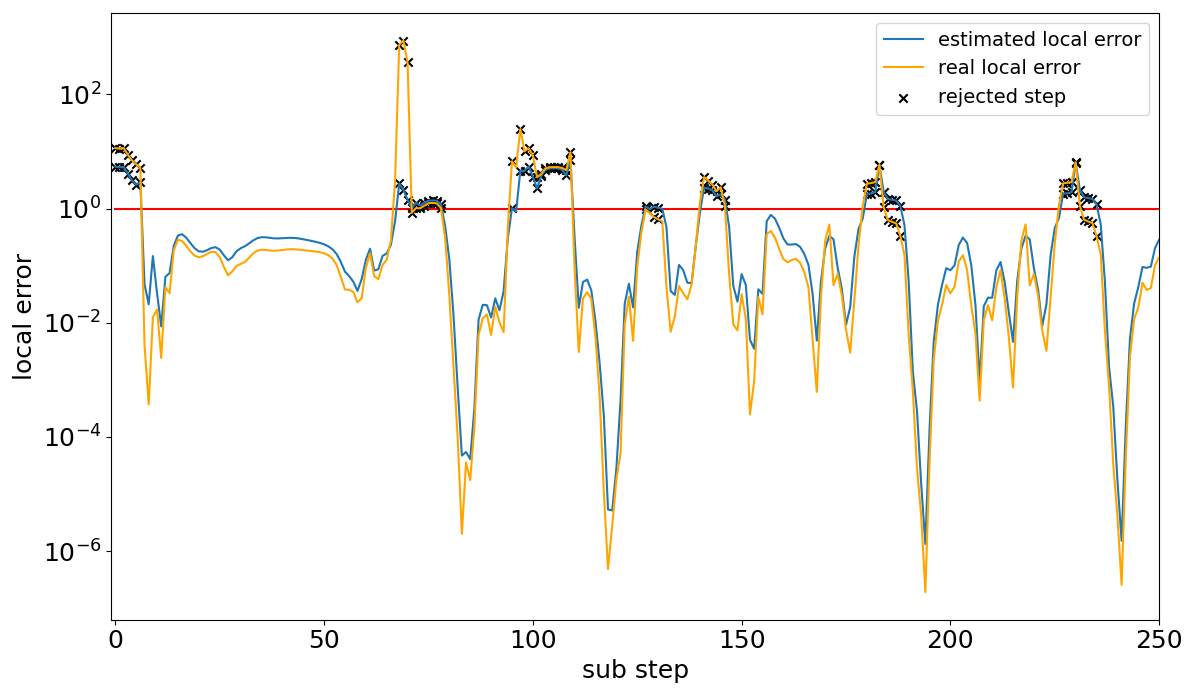
Figure 1 Comparison between the estimated local error of the embedded Rosenbrock solver (blue) and the more precise approximation of local error (orange) for the marine scenario. The figure shows a nearly constant overestimation of the local error for accepted steps. Moreover, regular sharp drops in the local error occur. Both findings mark potential for efficiency improvements. The red line marks the acceptance threshold of each sub-time step.

Changes in the lower growth limit factor q_min showed nearly no influence on the performance, mainly because the reduction factor r is the key parameter for step size reduction. Compared to the known default step size control proposed by Hairer et al. (1993), the reduction factor r is an addition in KPP. It helps decrease the step size faster in the very stiff scenarios we are working with. When the step size is rejected more than twice in a row, then the next rejected step size is multiplied by this factor; by default it is r=0.1. By looking at Fig. 2, one could assume that a smaller reduction factor may help to decrease the step size faster in the areas where it drops off drastically. Tests showed that this is true, but the difference is only marginal. Nevertheless, we found that in combination with a larger safety factor δ, the reduction factor may even be increased. In the marine scenario, this led to an additional 10 % reduction in function evaluations. However, in the megacity and forest scenarios, this also had no meaningful impact. The tests showed that there were no consistent performance changes in one direction for increases or decreases in the reduction factor, but overall, values in the range $r\in [\mathrm{0.05},\mathrm{0.2}]$ performed well.

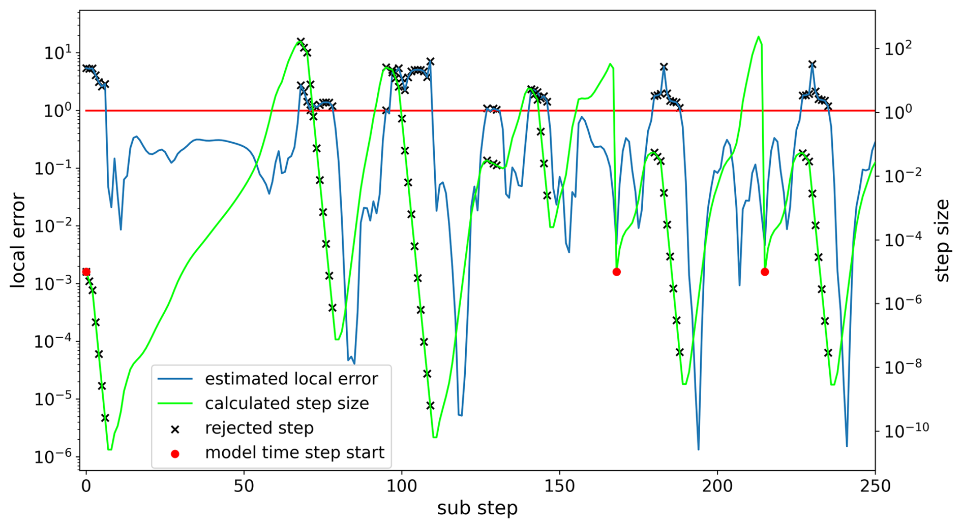
Figure 2 The estimated local error (blue) and the selected step size (green) for each substep of the marine scenario simulation. The strong local error dips occur when the step size increases after a strong decrease. This indicates that faster step size growth may be suitable. The red dots mark the beginning of a model time step. The first model step requires significantly more substeps than the other model steps.

Lastly, we did some rudimentary tests with the starting step size h_start. It is used at the beginning of each model step, so it can have a meaningful impact on the efficiency of the integration even though it is not part of the step size controller itself. Figure 2 shows that in the first model time step, the current value of 10⁻⁵ was too high because the controller started with multiple rejections. However, for the following model steps, the step size always grew at the beginning; thus higher values also seemed to be reasonable. Because of that, we tested lower and higher values, namely ${\mathrm{10}}^{-\mathrm{9}},{\mathrm{10}}^{-\mathrm{8}},{\mathrm{10}}^{-\mathrm{7}},{\mathrm{10}}^{-\mathrm{6}},{\mathrm{10}}^{-\mathrm{4}}$ and 10⁻³. Larger values resulted in unstable model runs, leading to crashes. On the other hand, smaller values yielded a slight increase in the number of function evaluations. Therefore, in short, changing this parameter did not help to increase the efficiency in our cases. Overall, the default value of 10⁻⁵ showed the best results, although better results may be achieved with an automatic starting step size selection (Watts, 1983).

3.2 Second-order controller

The adjustment of multiple heuristic parameters of the standard step size controller by Hairer et al. (1993) gave promising results. However, this makes adjusting the controller's behavior rather inconvenient and too specific for the ODE system at hand. In search of a more general and flexible step size control, we implemented the H211b controller by Söderlind (2003) from Eq. (6) and tested it with the same CAABA scenarios. The pseudocode of the implementation is shown in Appendix A.

We varied k over the range of [1.5,3], which equals the lower bound of $\frac{\widehat{p}+\mathrm{1}}{\mathrm{2}}$ and the default root exponent of $\widehat{p}+\mathrm{1}$. Since higher values of parameter b create a smoother and more robust step size sequence, which somewhat stands in contrast to a more efficient step size sequence, we decided to use the lowest possible value b=1 for our tests. Simulations with higher values for b always resulted in more function evaluations. Even though Söderlind (2003) recommended b>1, we did not encounter any issues with b=1. However, this should be kept in mind if stability issues arise in other cases.

Figure 5 shows that with decreasing values of k, the number of function evaluations dropped quite significantly in the megacity and marine scenarios. These reductions were about the same as with the increased safety factor in the default step size controller (cf. Fig. 3). Furthermore, the forest scenario also showed a meaningful reduction in the number of function evaluations, even though it is not as strong as in the two scenarios displayed. The marine scenario showed that setting k to the lowest possible value (1.5) might not be optimal because the error grew stronger compared to the computational saving. For the forest scenario, this value even increased the costs slightly. This leads to the conclusion that slightly higher values, around $k\approx \frac{\mathrm{2}}{\mathrm{3}}\left(\widehat{p}+\mathrm{1}\right)$, seem more appropriate as a rule of thumb.

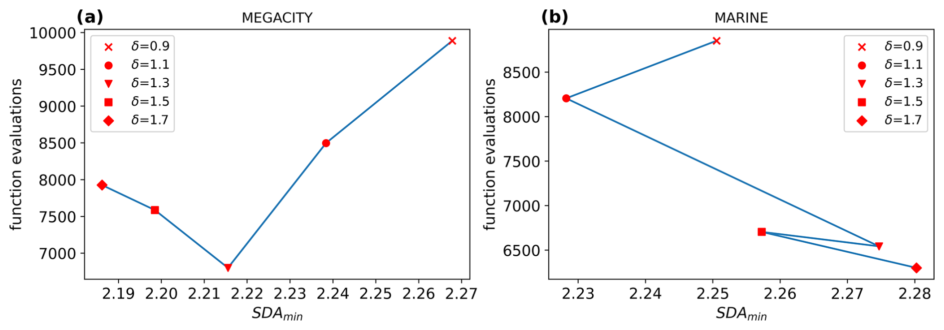
Figure 3 Work–precision diagrams for (a) the megacity scenario and (b) the marine scenario. Generally, a larger safety factor δ produces fewer function calls. For the megacity scenario, the SDA decreases slightly with each reduction in k. For the marine scenario, only δ=1.1 results in a decreased SDA. The computational amount could be decreased by up to 31 % for the megacity scenario and 26 % for the marine scenario, with δ=1.3.

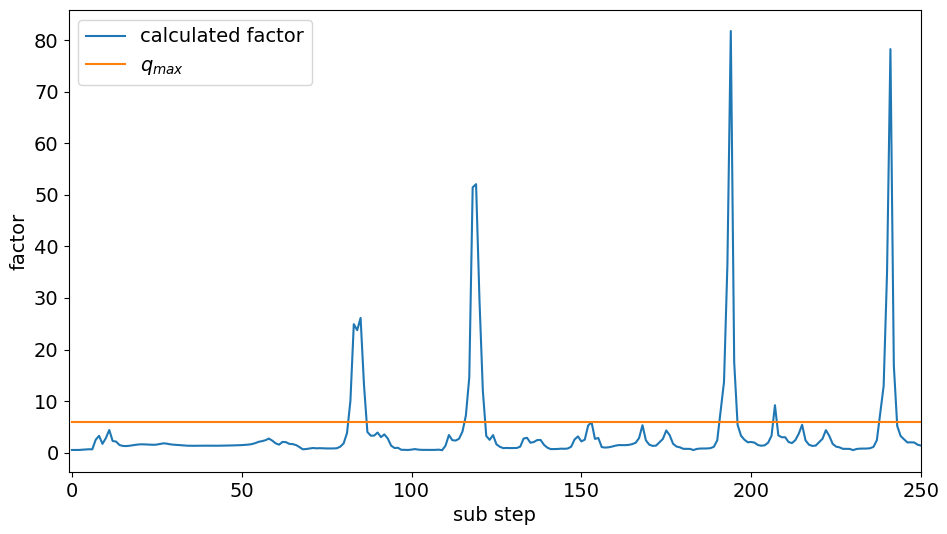
Figure 4 Visualization of the calculated growth factor (blue) that is limited by q_max (orange). The limit is only exceeded for a few substeps, but when it is, the value becomes much higher, up to 80. Exceeding the limit strongly correlates with the strong drops in the local error.

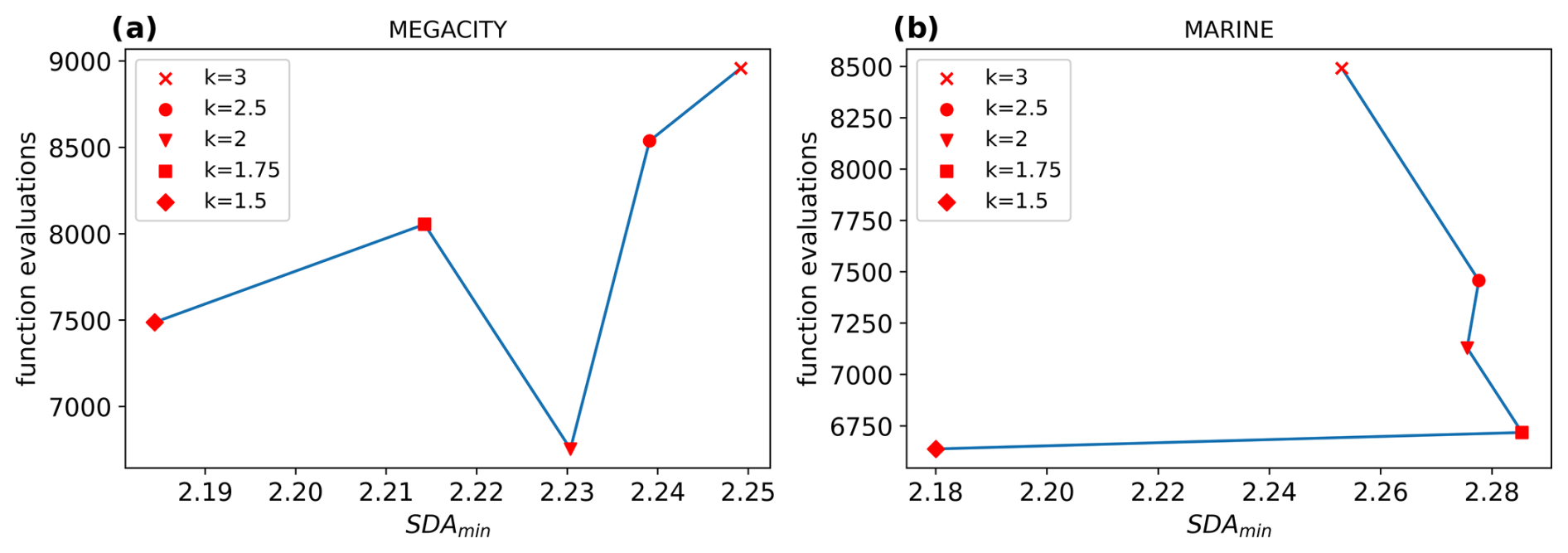
Figure 5 Work–precision diagrams for (a) the megacity scenario and (b) the marine scenario. Generally, lower values for k produce fewer function calls. For the megacity scenario, the SDA decreases slightly with each reduction in k. For the marine scenario, only k=1.5 results in a decreased SDA. The computational amount could be decreased by up to 31.7 % for the megacity scenario and 24.1 % for the marine scenario, with k=2 and k=1.75, respectively.

4 Step size control in the global model

We applied the findings of the CAABA simulations to the EMAC model and investigated if they yielded similar reductions in the number of required function evaluations. Here, we present the results of the 1 d global simulations with the setup described in Sect. 2.4. The controller parameters were changed for each submodel independently, and each simulation included only one parameter change.

4.1 First-order controller

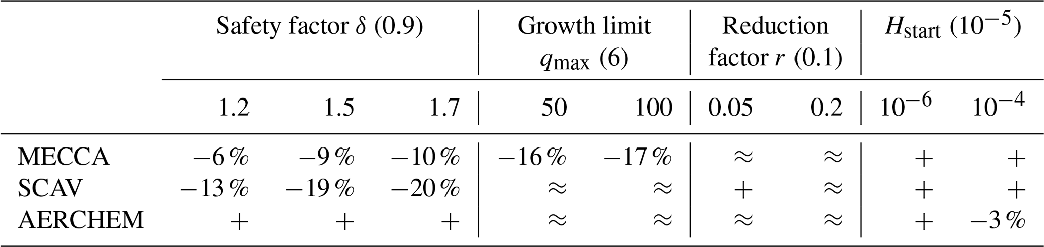
Starting with simulation parameters for MECCA, it could be observed that changes in the reduction factor and the starting step size did not result in fewer function evaluations. Modifications to all other parameters provided improvements. The changes in the safety factor resulted in up to 10 % fewer function evaluations, which is less than in the box model. Interestingly, the upper growth boundary q_max showed even more improvement with a reduction of about 17 %. In the box model, this parameter had nearly no impact. Overall, the efficiency gains were smaller than in the box model but still have a high potential to reduce the computational burden of long global simulations. Looking into the simulations with changed parameters for SCAV, the results did not differ too much from the MECCA results. Again, the reduction factor and the starting step size yielded no improvements, but here q_max also showed no decrease. The different safety factors resulted in reductions between 13 % and 20 %, which is slightly better than in MECCA. Lastly, we changed the parameters for AERCHEM. The results for the default controller showed nearly no improvements; the only change that resulted in a small decrease in the function evaluations of 3 % was the starting step size of 10⁻⁴. In contrast to the box model results, changing the safety factor increased the number of function evaluations. For the largest value, the increase was quite significant. The reasons for this might be the lower tolerance used by AERCHEM (10⁻³ instead of 10⁻²) and stronger chemical perturbations compared to the box model. A more detailed overview of the tests with the first-order controller can be seen in Table 3. Table C1 in Appendix C shows the workload for each ODE system.

Table 3 Overview of EMAC results for different first-order controller parameter values derived from the investigations of the box model. Concrete percentages are only displayed for meaningful reductions in the number of function evaluations. The percentage numbers refer to the reduction within the corresponding ODE system, not to the total accumulated number of function evaluations. The + symbol indicates an increase, and ≈ represents nearly no changes. Good improvements were achieved by increasing q_max and δ for MECCA and δ for SCAV but not for AERCHEM. The values in the brackets represent the default value of the parameter.

4.2 Second-order controller

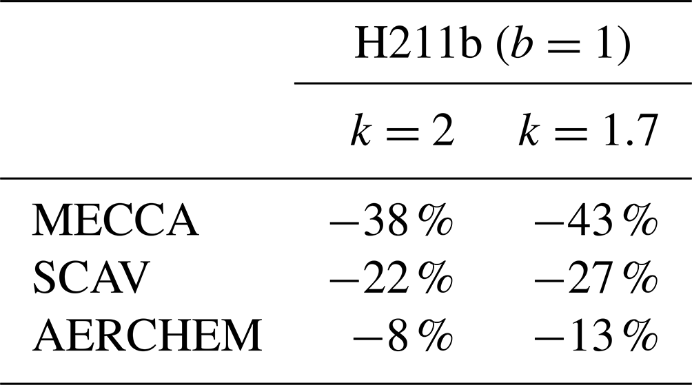
We performed the same 1 d simulations with the second-order controller. We tested k=2 and k=1.7 because these values cover the range where the best reductions in the box model investigations were found. A detailed overview of the impacts is presented in Table 4. For MECCA, up to 43 % fewer function evaluations were achieved, which was much better than the reduction in the default controller. For SCAV, the reduction with the second-order controller was also higher than with the first-order controller, with a 27 % reduction. Finally, for AERCHEM, it can be seen that with the H211b controller a reduction of 13 % was possible, with b=1 and k=1.7. In contrast to the first-order controller, the second-order controller showed significant improvements in this case. The comparison between the columns of Table 4 generally shows that a smaller value of k also performed better throughout for the global model simulations.

Table 4 Overview of EMAC results with the H211b controller, similar to Table 3. Overall, the H211b controller performed much better than the current controller and had the only meaningful improvement for AERCHEM.

In conclusion, we were also able to reduce the number of required function evaluations in EMAC simulations with the help of the CAABA investigations. However, in the global model simulations, the H211b controller was superior to the default controller, whereas for the box model, the performance gains were similar.

5 Long-term global simulations

Typically, global atmospheric simulations cover a period much larger than a single day. Therefore, there is a need to assess the accuracy of the results for much longer integration times. We hence made three 1-year simulations, as described in Sect. 2.4. We first highlight how much runtime can be saved with better parameters for the first-order controller and the second-order controller compared to the currently used setup over the longer simulation period. Secondly, we show that this was achieved with a minimal loss in the quality of the integration results.

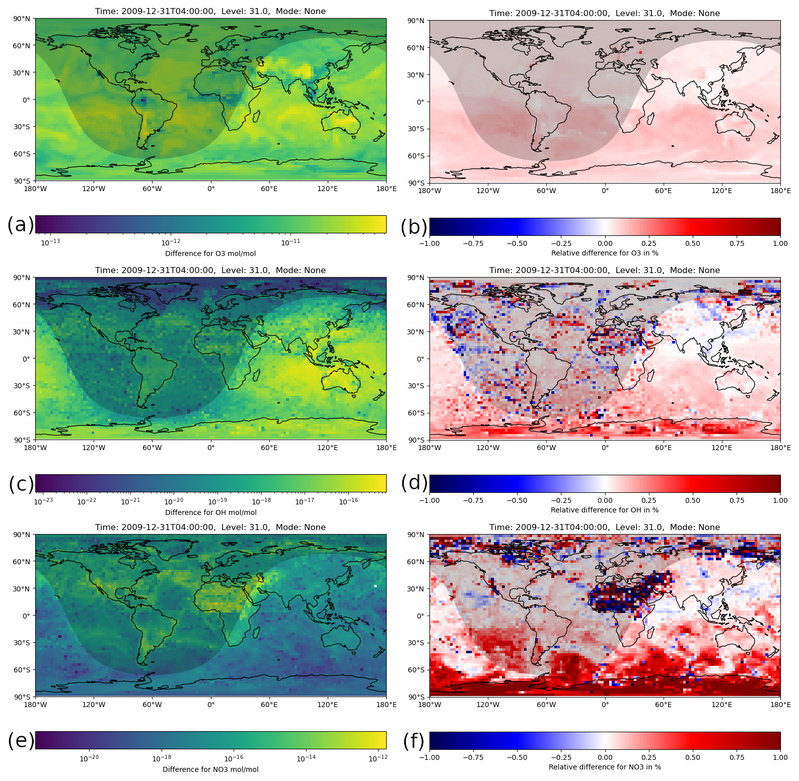
Figure 6 Instantaneous mixing ratio differences between the H211b and the reference 1-year simulations for the last simulation day (31 December 2009, 04:00:00 UTC). The shaded area represents nighttime. (a) Absolute difference for O₃. (b) Relative difference for O₃. All values are far below 1 %, which is below the relative tolerance used. (c) Absolute difference for OH. (d) Relative difference for OH. Nearly all values are below 1 %. A few boxes slightly exceed this value, but only in nighttime areas with small absolute values. (e) Absolute difference for NO₃. (f) Relative difference for NO₃. Again, most values are below 1 %, but some larger areas exceed this value. There, a few boxes go up to 20 %.

5.1 Runtime comparison

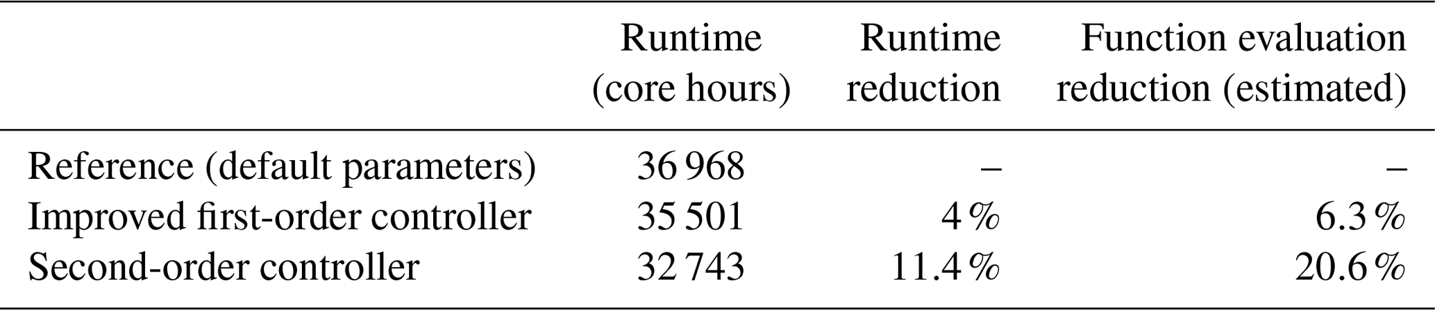
Table 5 gives an overview of the required computation time for each simulation and the reduction that was achieved with the new changes. The results show that with the simple parameter changes in the current step size controller, a runtime reduction of roughly 1500 core hours was achieved compared to the reference, which equals a reduction of 4 %. The reference simulations used the default parameters presented in Sect. 3.1.2 for each submodel, while in the improved first-order controller, q_max=100 was used for MECCA, δ=1.5 for SCAV and $h_{\mathrm{start}}={\mathrm{10}}^{-\mathrm{4}}$ for AERCHEM. With the newly tested H211b controller, the reduction was about 3 times as high. The corresponding simulation required over 4000 core hours less than for the reference one, which is about 11.4 %. In addition to the runtime, the last table column also shows the estimated overall reduction for the number of function evaluations, which was up to 20.6 % with the second-order controller. Given that output was only written every 23rd hour, this reduction can only be estimated. Furthermore, it should be noted that the percentage runtime reduction will always be below the function call reduction because the model calculates many processes that are not influenced by our changes, like I/O or atmospheric physics.

Table 5 Comparison of runtimes for 1-year EMAC simulations with the reference and two optimized controllers. The reference is the first-order controller with default parameters. The improved first-order controller has the following modified parameters: q_max=100 was used for MECCA, δ=1.5 for SCAV and $h_{\mathrm{start}}={\mathrm{10}}^{-\mathrm{4}}$ for AERCHEM. The second-order controller was used with b=1 and k=1.7 for MECCA, SCAV and AERCHEM.

5.2 Error analysis

It is important to note that we do not have a meaningful reduction in the accuracy of the calculated chemical abundances. In this respect, we want to stress that not a single change was made that would influence the precision control behavior of the integrator. The controller changes only influenced the calculation of the step size candidate to use for the next step. The estimation of the local error and the verification that the step calculated last fits the desired tolerance were not changed in any way. Nonetheless, given the complexity of the chemical ODE systems and all the uncertainties in such models, we carried out a few investigations with respect to the quality of the results.

Given the superiority of the H211b controller, the following results only refer to a comparison between the 1-year simulation with this new controller and the reference simulation. Note that this comparison does not reflect a precision comparison as for CAABA, where we used a Radau integrator with a much stricter tolerance as reference. A global simulation with the Radau integrator would simply not be feasible with our setup for this time span.

Figure 6 shows the absolute and relative difference for the main atmospheric oxidants, O₃, OH and NO₃, in the gas phase. All plots show ground level, instantaneous values from the last model time step. For ozone, it can be seen that the relative difference was well below 1 % across the whole globe and thus smaller than the relative tolerance used.

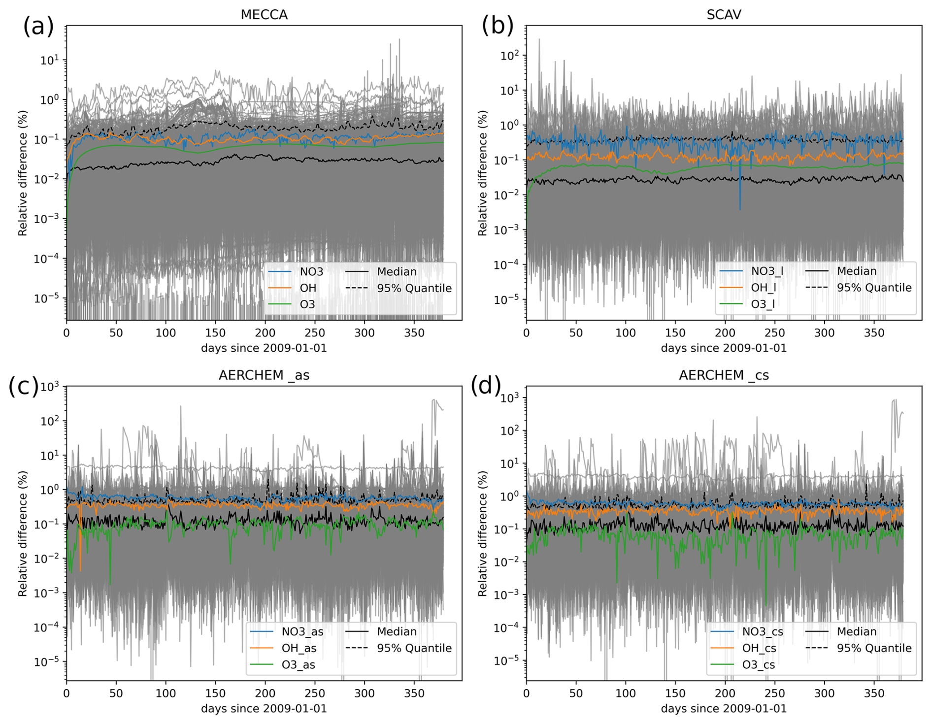
Figure 7 Time series of the relative differences for the tropospheric globally averaged concentrations for all species between the reference and the H211b global 1-year simulations.

For OH, the relative difference was overall still below 1 %, but some areas had higher values than others. For example, above northern Africa the differences were all comparatively high, and a handful of boxes even slightly exceeded 1 %. However, this is in no way significant because they mainly occurred in nighttime areas where OH was very close to zero. Because of this, the absolute difference was also very small, which makes the relative error very sensitive to small changes.

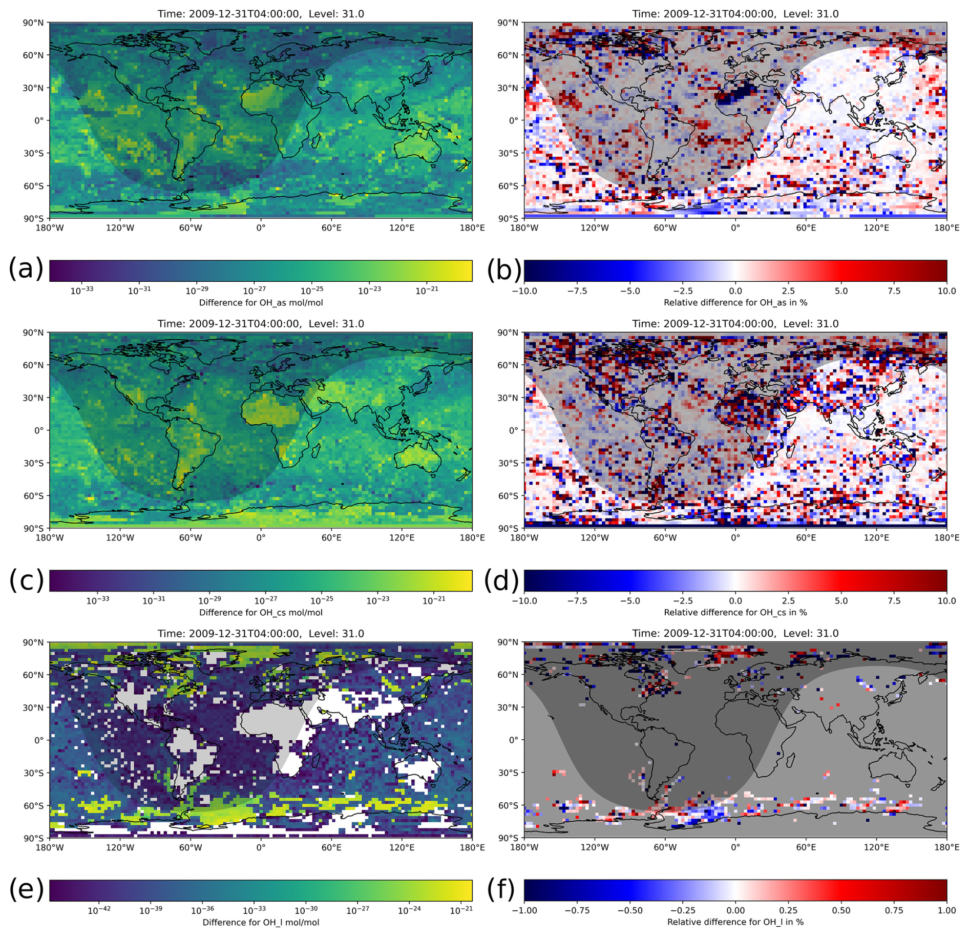
Figure 8 Instantaneous mixing ratio differences between the H211b and the reference 1-year simulations for the last simulation day (31 December 2009, 04:00:00 UTC). The shaded area represents nighttime. Absolute differences (a, c, f) and relative differences (b, d, e) for OH in the accumulation-aerosol mode, the coarse-aerosol mode and cloud droplets, respectively. Higher mixing ratios have a relative difference below 1 %. For very small mixing ratios, the high relative difference is a result of single-precision limitations.

For NO₃, the relative error was below 1 % in most areas. However, there were a few regions where it exceeded 1 %, notably northern Africa. Most of these values were only slightly higher, but a handful of outliers were above 10 % or even 20 %. For earlier time steps, similar relative differences were produced in this area, especially during nighttime. This indicates that the observed difference was not caused by error propagation.

Following this, Fig. 7 shows the time series of the relative differences in the mean concentrations within the tropospheric levels. O₃, OH and NO₃ are highlighted, while all other species are shown in gray. In addition, the black lines mark the median and the 95% quantile levels. It can be seen that for the vast majority of species, the differences were always below the desired 1 % tolerance, especially for the gas-phase species in MECCA. Species from SCAV and AERCHEM produced slightly higher differences, but only a few outliers were above 1 %. Furthermore, the differences did not grow over time. This also supports the suggestion that the quality of the results did not decrease. Larger deviations for NO₃ are not surprising, given that NO₃ chemistry is coupled directly to extremely fast phase-transfer and dissociation reactions of N₂O₅ in cloud droplets and aerosols.

Because the mechanism used simulates more than just gas-phase chemistry, we also looked into the cloud and aerosol-phase mixing ratios, focusing on OH. Figure 8 shows absolute and relative differences for the cloud phase (OH_l) and aerosol phase in the accumulation-soluble mode (OH_as) and coarse-soluble mode (OH_cs). The mixing ratios in these phases were generally much lower and were distributed on a wider range of values than in the gas phase. This made the error investigation and interpretation of the results more complex.

For the cloud-phase chemistry in particular, the relative difference seemed to be extremely high for the majority of the grid boxes. The reason for this is the very small mixing ratios and the correspondingly very small absolute differences, down to 10⁻⁴⁴. For single precision, values below 10⁻³⁸ are represented as subnormal numbers, which have a significantly reduced precision (IEEE, 2019). Furthermore, the data also contained missing values for areas without clouds. We therefore greyed out areas without clouds and with concentrations below 10⁻³² in Fig. 8f. In areas with relevant mixing ratios, colored in yellow and green, the relative difference was below 1 %.

The aerosol chemistry showed overall higher relative differences compared to the gas phase, which is why we changed the displayed range to 10 %. A few boxes also exceed this value; however the vast majority is still below 10 %, and over 75 % of the boxes are even below 1 % relative error. For completeness, we added the relative differences for ${\mathrm{NO}}_{\mathrm{3}}^{-}$ and Cl⁻ (Fig. S1 in the Supplement) and for ${\mathrm{SO}}_{\mathrm{4}}^{\mathrm{2}-}$ and ${\mathrm{NH}}_{\mathrm{4}}^{+}$ (Fig. S2) in their respective aqueous and aerosol phases in the Supplement.

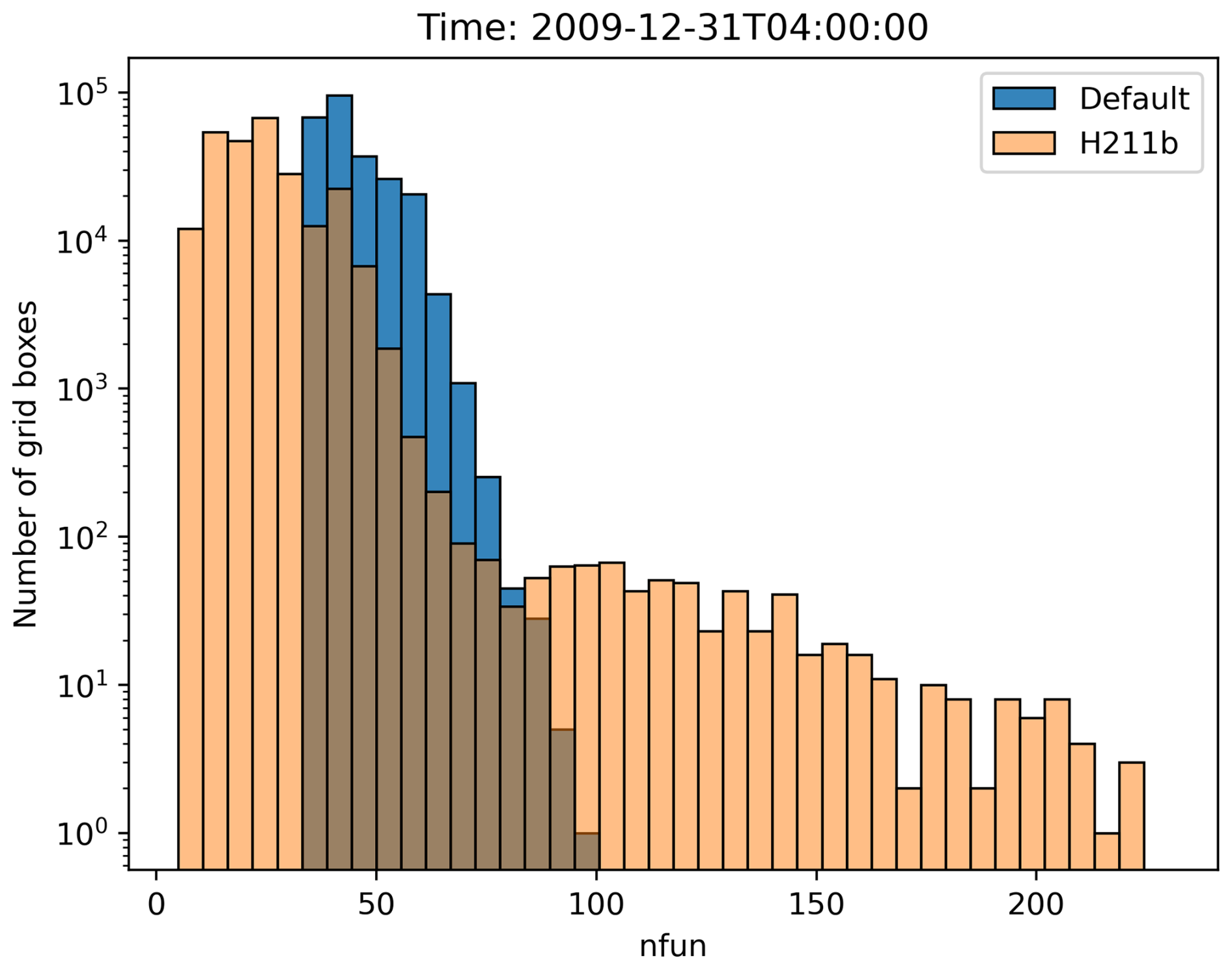
Figure 9 The histogram shows the number of grid boxes (y axis, logarithmic scale) that require a certain number of function evaluations (x axis). The blue bars represent the reference 1-year simulation with the default parameters, and the orange bars represent the 1-year simulation with the H211b controller.

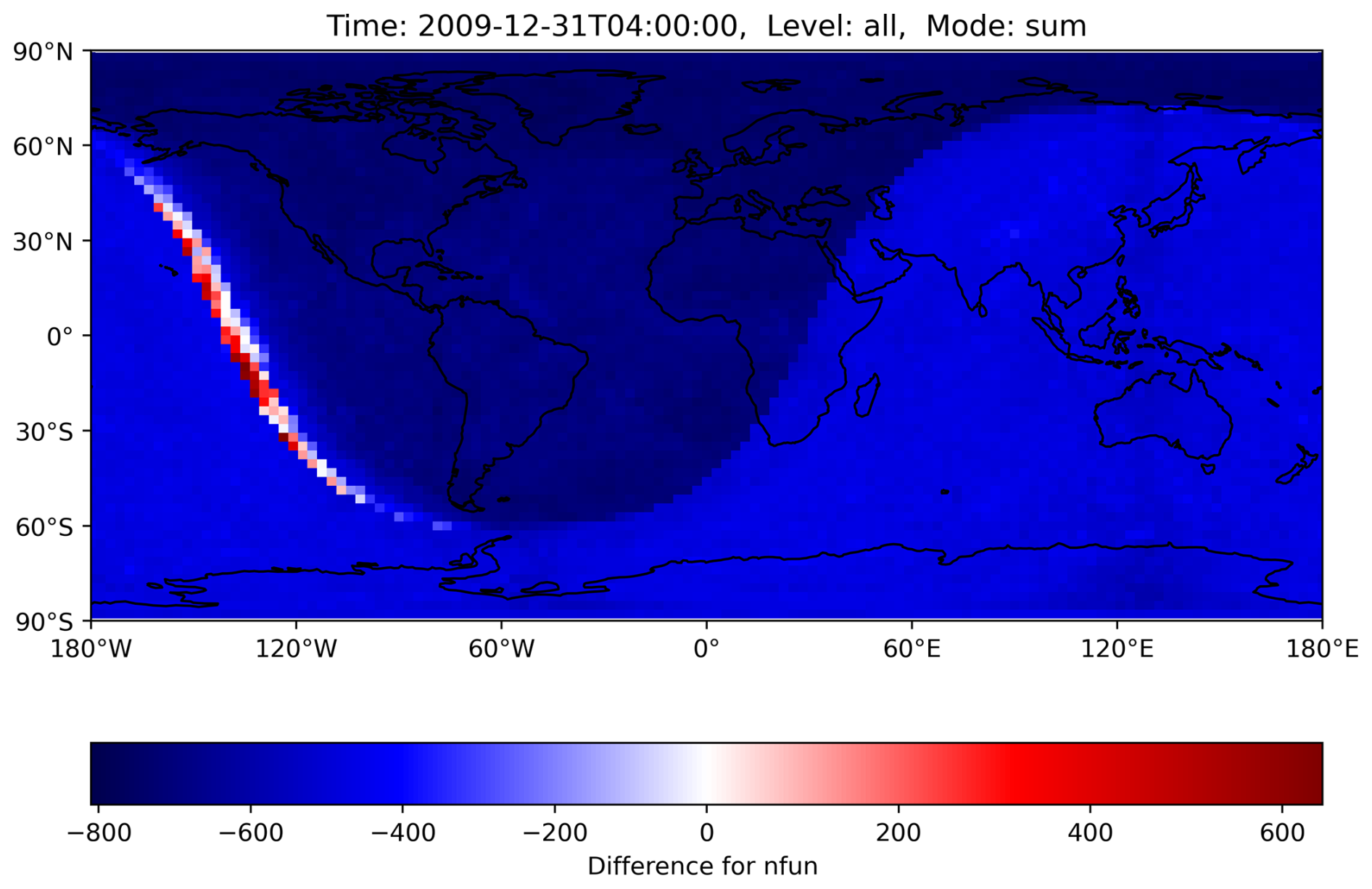
Figure 10 The number of function evaluations for the MECCA ODE system is summed up across all levels for the reference and the H211b simulation, with the difference calculated afterward. The dominating negative values show a decrease with the new controller. The few red boxes mark an increase in this area. Load imbalance could increase in the worst case if many red boxes are calculated by the same CPU core. However, in practice, there is no meaningful impact. GPU usage should further decrease this issue. The shaded area represents nighttime.

6 Load imbalance

One aspect that differs from the CAABA simulations was that EMAC simulations heavily utilize parallelization by distributing grid cells onto multiple CPUs and their cores. For the box model, we had no parallelization. This made the number of function evaluations a perfect metric that solely represents the workload of the chemical ODE system. In the case of the global model, the parallelization could cause the additional issue of unequal distribution of workload (load imbalance). In MESSy, the parallel decomposition depends on the dynamical core that is used (ECHAM5 in the EMAC configuration). The model grid is split horizontally by selecting the number of processes in lat–long rectangular sets of grid points. Two diametrically opposed sets are assigned to one processor. This is done to counteract the load imbalance associated with radiation transfer and photochemistry (Christou et al., 2016).

With the new changes, we observed that while most areas require fewer function evaluations, there are very few boxes where the number of function evaluations increased, as can be seen in Fig. 9. In the worst case, this could lead to an overall increase in load imbalance and thus computation time if a single CPU core gets all boxes where the number increases, as all other cores would need to wait, without any overall benefit. Nevertheless, as seen in the runtime reductions from Sect. 5, this problem did not occur in our simulations, or at least not to a meaningful extent. However, it could occur for a different setup and should be kept in mind. As shown in Fig. 10, an increase in the number of function evaluations (the corresponding variable is called nfun) only happened in areas where day–night transitions occurred. The grid decomposition algorithm does distribute these grid boxes with high workload evenly across the cores. The unintended worsening of the load imbalance is likely associated with the rapid change in chemical regime from OH- to NO₃-dominated chemistry. NO₃ chemistry is closely coupled to N₂O₅, which is very reactive in both the gas and the aqueous phase, leading to enhanced ODE stiffness. This issue is already known. At dusk and dawn the strong perturbation to the chemical regime via changing photolysis rates enhances the ODE stiffness, and the chemical solver therefore needs the largest number of substeps for the integration (Christou et al., 2016).

Nevertheless, porting the chemical solver to GPUs makes the load imbalance a minor issue because of the much higher degree of parallelization. The integration of the chemical ODE system can be ported to GPUs with a Fortran-to-CUDA parser (Alvanos and Christoudias, 2017; Christoudias et al., 2021).

7 Conclusions

This work highlighted that the commonly used default step size controller for Rosenbrock solvers poses many inefficiencies in the context of atmospheric chemical ODE systems. For box model simulations with CAABA, we found a near-constant overestimation of the local error, as well as regular decreases to very small values. Both indicated the possibility for improvement by using a more efficient step size selection. Based on this, we also showed that we were able to decrease the workload of the ODE solver by simply changing the heuristic parameters of the controller. Furthermore, for the global model EMAC, even better results were achieved with the new H211b controller, where the computation time of a simulation with multiphase chemistry was reduced by 11.4 %. Lastly, we also ensured that the results of the solver continue to be trustworthy in terms of accuracy.

Given the good performance, we recommend this controller as the new default choice. Generally, it could be worthwhile to test higher-order step size controllers, such as that of Söderlind (2003), for further speedups of atmospheric chemistry simulations. Additional efficiency gains might be achieved by applying the quasi-steady-state approximation (Turanyi et al., 1993, QSSA;) for stiffness reduction. This option is available in our modified Rosenbrock integrator as well and allows for a dynamical choice of the initial step size. However, this option is recommended only for gas-phase chemistry calculations, and its impact on accuracy and efficiency still needs to be assessed.

Appendix A: Controller implementations

Algorithm A1 Pseudocode of the default first-order controller implementation.

Algorithm A2 Pseudocode of the H211b controller implementation.

We present the pseudocode of our implementations of the standard first-order controller and the second-order H211b controller. Our default controller implementation only differs with respect to two minor aspects compared to the one in Hairer et al. (1993). Given that the error tolerances are part of the local error estimation (see Eq. 5), the value of ε in the numerator has to be set to 1. Furthermore, we highlighted the use of a reduction factor that is applied when a step size is rejected twice or more in a row. For the H211b controller, we also make use of the reduction factor. Besides initializing two new variables, we only need to change the line of code that calculates the growth factor. The factor calculation is nearly identical to Eq. (6), with only two minor modifications. Instead of storing the last step size, the quotient $\frac{h_i}{h_{i-\mathrm{1}}}$, which equals the last growth factor, is stored in a new variable. In the numerator, ε is again set to 1 for the same reason as above.

Appendix B: Single-digit accuracy (SDA)

Table B1 Median, mean and lowest single-digit accuracy for each box model scenario.

As a measure of accuracy, we used single-digit accuracy (SDA), similar to Sandu et al. (1997b). It expresses the number of significant digits and can be calculated in the following way:

$$\begin{array}{}\text{(B1)}& \mathrm{SDA}=-{\log }_{\mathrm{10}}\left(\mathrm{relativeError}\right).\end{array}$$

To calculate the relative error of the CAABA results, we took the reference values from a fully implicit Radau-5 integrator with a relative tolerance of 10⁻⁷. We calculated the SDA of the mean, median and largest relative error over a selection of 86 components. The aspired mean should be a value of approximately 2, but the mean and median accuracies were much better, as shown in Table B1. In the work–precision diagrams, we used SDA_min, which reflects the least precise component with the largest relative error. Only the forest scenario had an SDA_min below 2; all other values were noticeably above this value.

Appendix C: Workload of each ODE system in EMAC

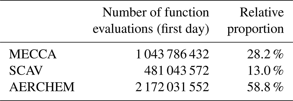
Table C1 shows the number of function evaluations needed for each system for the first simulation day of the global reference run. AERCHEM requires the most function evaluations, totaling about 2.17 billion, followed by MECCA with just over 1 billion. Finally, SCAV requires the least number of function evaluations, totaling 481 million.

Table C1 Comparison between the amount of work required in the three ODE systems in our global model setup.