Modelling emission and transport of key components of primary marine organic aerosol using the global aerosol–climate model ECHAM6.3–HAM2.3

Primary marine organic aerosol (PMOA) contributes significantly to the aerosol loading over remote oceanic regions, where sea spray dominates aerosol production in the lower troposphere, and plays an important role in aerosol–cloud–climate interactions. The sea–atmosphere transfer of organic components depends on their abundance at the ocean surface and their physicochemical characteristics. We introduce a novel approach for representing the ocean concentration of the most abundant organic groups in seawater that are relevant for aerosols. By apportioning the phytoplankton-exuded dissolved organic carbon, modelled in the biogeochemistry model FESOM2.1–REcoM3, three biomolecule groups are computed (dissolved carboxylic acidic containing polysaccharides (PCHO), dissolved combined amino acids (DCAA), and polar lipids (PL)). The transfer of these marine groups to the atmosphere is represented by the OCEANFILMS (Organic Compounds from Ecosystems to Aerosols: Natural Films and Interfaces via Langmuir Molecular Surfactants) parameterization which is implemented in the aerosol–climate model ECHAM6.3–HAM2.3 to represent the emission and transport processes in the atmosphere. The concentration of biomolecules in the ocean serves as the bottom boundary condition for the PMOA simulation within the aerosol model. Among the simulated organic groups in seawater, modelled PCHO is the most prevalent, followed by DCAA and PL. Conversely, PL contributes the most to the organic matter in aerosols, given the high air–seawater affinity of lipids compared to the other groups. Biomolecules exhibit minor variations in equatorial waters, whereas strong seasonal patterns are observed towards the polar regions. The global aerosol model simulations indicate that PMOA emission fluxes are primarily influenced by marine biological activity and surface wind conditions. Based on the most comprehensive evaluation to date, the computed levels of biomolecules in the ocean and species-resolved PMOA concentrations are compared with ground-based measurements across the globe. The comparison shows a reasonably good agreement, given the uncertainties in model assumptions and measurements. Model biases in the representation of the marine organic aerosol groups are caused by uncertainties in the aerosol-process representation and the simulated sea salt concentrations. A comparison with a set of long-range in situ aircraft measurements indicates that by including PMOA in the model, the representation of organic aerosols in the southern oceans is significantly improved.

1 Introduction

Oceans are a major source of natural aerosols (O'Dowd et al., 1997; Simó, 2004; Lewis and Schwartz, 2004; Galí et al., 2018; Rinaldi et al., 2020). Wind-generated sea spray aerosol (SSA) particles predominate in the marine boundary layer (Blanchard and Woodcock, 1980; O'Dowd et al., 1997; Lewis and Schwartz, 2004). They therefore significantly influence the climate system through aerosol–radiation and aerosol–cloud interactions in remote marine and coastal regions (Pandis et al., 1994; Murphy et al., 1998; Carslaw et al., 2013; Vergara-Temprado et al., 2017).

Multiple experimental studies simulating air bubble bursting have demonstrated that marine organic constituents are co-emitted with sea salt in sea spray (Keene et al., 2007; Facchini et al., 2008; Schmitt-Kopplin et al., 2012). This so-called primary marine organic aerosol (PMOA) emitted directly this way dominates the sub-micron range of the sea spray particle size distribution (Facchini et al., 2008; Gantt et al., 2011; Gantt and Meskhidze, 2013). Nonetheless, organics also contribute to the chemical composition of the coarse mode of sea salt aerosol particles (Hawkins and Russell, 2010; Russell et al., 2010; Leck et al., 2013; Zeppenfeld et al., 2021).

Many organic compounds detected in ambient marine samples are found to be highly enriched in the surface microlayer (SML) with respect to bulk water (Engel et al., 2017; Pinxteren et al., 2017; Triesch et al., 2021a, b; Zeppenfeld et al., 2023). The SML is the uppermost layer of the ocean, which often contains high concentrations of organic compounds that cover the surface of rising bubbles before bursting (Stefan and Szeri, 1999; Sellegri et al., 2006; Bigg and Leck, 2008). The characterized fraction of organic matter in the ocean is dominated by lipid-like, polysaccharidic and proteinaceous compounds (Wakeham et al., 1997; Repeta, 2015) that have also been detected inside aerosol particles (Frossard et al., 2014; van Pinxteren et al., 2023). The formation of PMOA is determined by the physicochemical properties of marine organic compounds, with the transfer from bulk water to SML to the atmosphere occurring in a chemo-selective manner (Facchini et al., 2008; Schmitt-Kopplin et al., 2012; Burrows et al., 2014). Highly surface-active molecules are preferably transferred compared to non-surface-active constituents. Thus, a differential enrichment is found in the aerosols compared to their analogues in seawater (Rastelli et al., 2017; van Pinxteren et al., 2023).

For a long time, there has been a high level of interest in the modelling of the emission, transport and physicochemical properties of PMOA in the context of aerosol–climate studies (O'Dowd et al., 2008; Vignati et al., 2010; Long et al., 2011; Albert et al., 2012; Gantt et al., 2012a; Vergara-Temprado et al., 2017). Various parametrizations, based on chlorophyll-a (chl-a) ocean concentration as a proxy for marine biological activity, have been used to account for wind-driven emissions of PMOA (O'Dowd et al., 2008; Gantt et al., 2011; Long et al., 2011; Rinaldi et al., 2013). Nevertheless, chl-a does not correlate with the organic fractions in aerosol particles in some regions (Prather et al., 2013; Collins et al., 2016), especially in oligotrophic waters. Hence, a more physically based framework to parameterize the coverage of surfactants on the bubble film and the relative enrichment in the aerosols was introduced by Burrows et al. (2014). The scheme requires input data that account for the presence of the most abundant macromolecules in the ocean. To this end, an ocean biogeochemistry model is needed to compute these quantities (Burrows et al., 2014; Ogunro et al., 2015).

Both methods of estimating PMOA mass fractions have been included and validated in global models (Meskhidze et al., 2011; Gantt et al., 2012b; Gantt and Meskhidze, 2013; Huang et al., 2018; Han et al., 2019). Recently, Zhao et al. (2021) found that the scheme by Burrows et al. (2014) yields an improvement in the representation of PMOA compared to a chl-a-based approach. Some modelling studies have additionally implemented the ability of PMOA to serve as ice nucleating particles (INPs) based on empirical formulations (Wilson et al., 2015; DeMott et al., 2016; McCluskey et al., 2018b). Special attention has been given to the significance of PMOA in the climate system as relevant INPs and, to a lesser extent, as cloud condensation nuclei (CCN), especially over remote marine environments (Gantt et al., 2012b; Burrows et al., 2013; Yun and Penner, 2013; Huang et al., 2018; Vergara-Temprado et al., 2018; Zhao et al., 2021; Burrows et al., 2022). The characteristics of the chemical compounds are also assumed to be important for their ice formation potential. There is evidence of high ice activity for marine polysaccharidic and proteinaceous compounds compared to other measured organic groups (McCluskey et al., 2018a; Alpert et al., 2022). Thus, representing PMOA as an independent component is crucial to establishing a solid foundation for future research on the climate impact of these biological compounds, particularly their effects on mixed-phase clouds.

To further investigate the occurrence of different PMOA species in various climate regions, we implement the sophisticated PMOA emission scheme by Burrows et al. (2014) in the global aerosol–climate model ECHAM6.3–HAM2.3 (Tegen et al., 2019). With regard to the marine boundary conditions, an approach for calculating the most important organic compounds in the ocean is introduced. In this approach, the contribution to the dissolved organic carbon (DOC) from the phytoplankton exudation is considered in contrast to carbon release via cell lysis by Burrows et al. (2014). The approach is based on simulation results from the detailed marine biogeochemical model FESOM2.1–REcoM3 (Gürses et al., 2023). This open-source marine biogeochemistry model allows for regional grid refinement, which improves the spatial and temporal representation of ocean biogeochemical processes, such as the evolution of phytoplankton blooms. This provides the basis for future high-resolution and species-resolved PMOA modelling studies to improve the model representation and understanding of marine aerosols and their interactions with different cloud types.

In this work, the so-extended aerosol–climate model is thoroughly evaluated against observations worldwide, and the results are analysed globally in terms of temporal and spatial patterns. Through a component-specific description for ground-based observations, a comprehensive assessment of the total PMOA can be achieved.

The paper is organized as follows. Section 2 introduces the approach considered to compute the organic aerosol mass fraction and the concentration of the biomolecules in the ocean. Section 3 presents a description of the aerosol–climate model, the aerosol model setup, and experiments. Section 4 describes the observational data used for the evaluation. Sections 5 and 6 discuss the model results and the comparison with measurements focusing on marine biomolecules at the sea surface and the associated aerosol emissions and transport, respectively. Finally, Sect. 7 summarizes and draws the conclusions of this work.

2 Modelling marine organic aerosol emissions and marine biomolecules

This section outlines the method used to determine the organic aerosol mass fraction and quantify biomolecule concentrations in the ocean, which is used in the aerosol–climate model simulations to account for species-resolved PMOA. To represent the mass fraction in marine nascent aerosol, we base our calculations on OCEANFILMS (Organic Compounds from Ecosystems to Aerosols: Natural Films and Interfaces via Langmuir Molecular Surfactants; Burrows et al., 2014). For the present study, we included minor adaptations to the scheme. A detailed description of the assumptions made here together with the calculation of the marine biomolecule groups in the ocean is given in the following sections. Figure 1 shows a condensed illustration of the model components of this study for all compartments and encapsulates what is presented in Sects. 2–4. In addition, the computed and analysed parameters in the results sections are also included in Fig. 1.

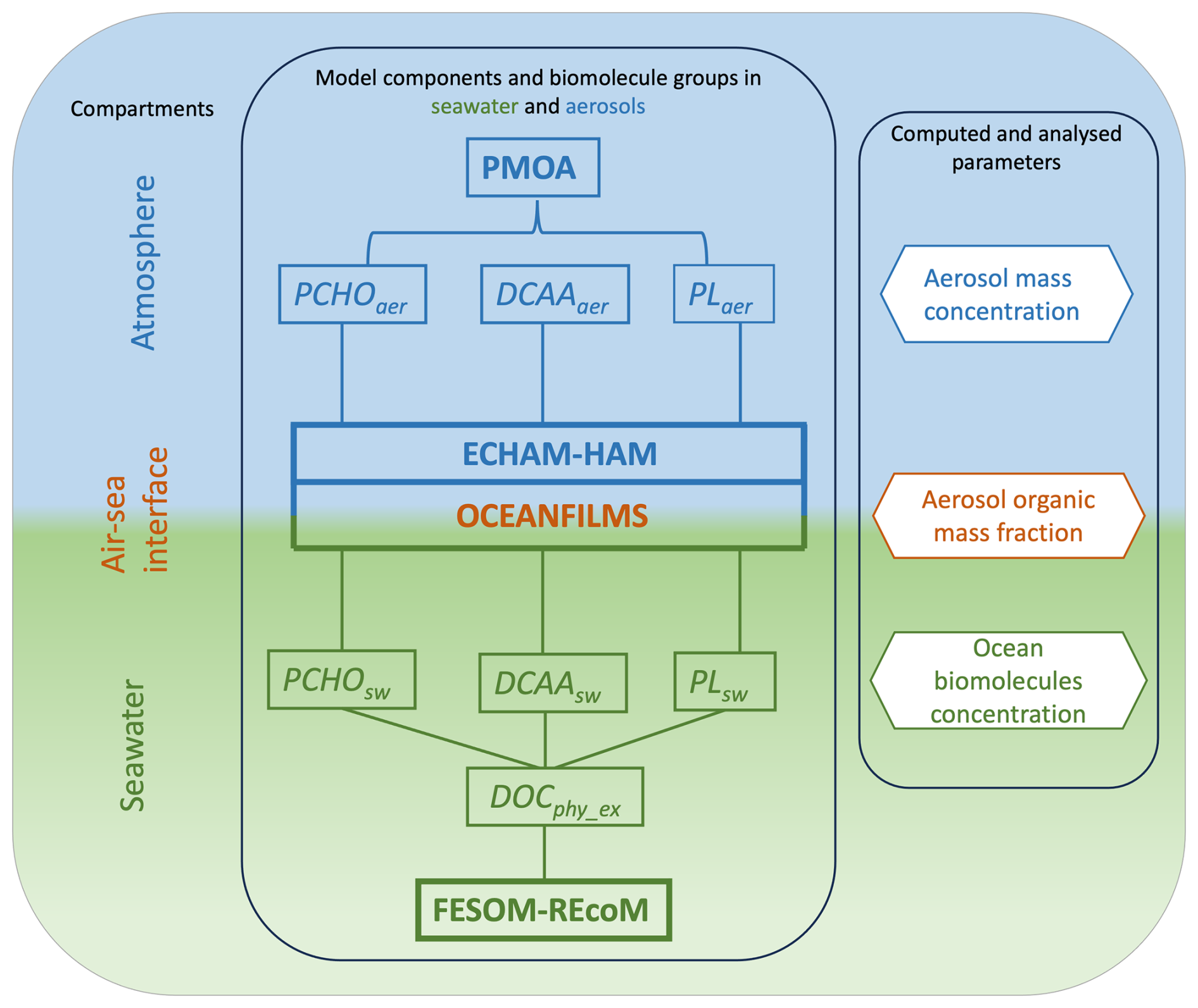
Figure 1 Schematic of the main modelling components considered in this study for simulating the biomolecules in seawater and their transfer to the atmosphere. Note that FESOM2.1–REcoM3 model data are used in offline mode and the modelled biomolecule groups serve as bottom boundary conditions of the integrated component OCEANFILMS + ECHAM6.3–HAM2.3. See Table 2 for the compound abbreviations.

2.1 PMOA emission parameterization

OCEANFILMS is a modelling framework that represents the sub-micron organic mass fraction in sea spray aerosol (air–sea interface compartment of Fig. 1). It is based on the Langmuir isotherm to represent the adsorption at bubble surfaces of the marine organic matter, which is apportioned into several classes. They include lipid-, polysaccharide-, protein-, humics-, and processed-like mixtures. The last two, humics- and processed-like mixtures, describe the recalcitrant DOC at the ocean surface, which is the DOC fraction that accumulates due to its resistance to rapid bacterial degradation (Hansell et al., 2012). These classes possess differing physicochemical characteristics: molar weight (MW_i), surface area (A_i), carbon concentration in seawater (C_i), and Langmuir adsorption (α_i). C_i and α_i regulate the bubble fractional surface coverage (θ_i). Note that i stands for the different classes. In combination with the bubble coating parameter (n=2, equivalent coverage of the interior and exterior of the bubble), the mass on the bubble surfaces (M_i) for each class can be computed as

$$\begin{array}{}\text{(1)}& M_i=n{\mathit{\theta }}_i{\displaystyle \frac{{\mathrm{MW}}_i}{A_i}}.\end{array}$$

Since PMOA and sea salt (SS) are emitted together, they make up the total mass of sea spray aerosol (SSA) (M_SSA). The organic mass fraction (OMF_i) is then calculated based on the mass per bubble surface area of the individual macromolecule group (M_i) and of sea salt (M_SS):

$$\begin{array}{}\text{(2)}& {\displaystyle }{M}_{\mathrm{SSA}}=M_i+M_{\mathrm{SS}},\text{(3)}& {\displaystyle }{\mathrm{OMF}}_i={\displaystyle \frac{M_i}{M_i+M_{\mathrm{SS}}}},\end{array}$$

where M_SS is assumed to be constant with a value of $\mathrm{3.59}\times {\mathrm{10}}^{-\mathrm{3}}$ g m⁻².

The organic carbon aerosol enrichment is a result of the differing properties of the macromolecules in seawater that regulate their transfer to the atmosphere (Burrows et al., 2014). Despite lipids having the lowest concentration in the ocean, their surface affinity and competitive adsorption favour their presence at the air–water interface (Frka et al., 2012) leading to higher aerosol enrichment compared to other macromolecules. Polysaccharide and protein surface affinity, on the other hand, is lower, limiting their transfer to the aerosols, with enrichment factors 2 orders of magnitude smaller than that for lipids (van Pinxteren et al., 2023). Lastly, humic- and processed-like mixtures have very low surface affinity, and, compared to the other classes, their contribution to the marine organic aerosol mass fraction may be negligible (Burrows et al., 2014). Hence, neglecting the recalcitrant portion of DOC will not impact the OMF estimations and is therefore not considered in this study.

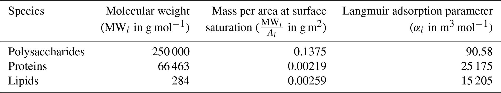
In the current study we account for the presence of three main biomolecule groups that represent a portion of the lipid-, protein-, and polysaccharide-like classes. We focus on the contribution of extracellular DOC from phytoplankton, apportioning the organic matter into the most abundant biomolecule groups in seawater based on a closure approach that will be introduced in Sect. 2.3 (seawater compartment in Fig. 1). In this respect, our approach differs from Burrows et al. (2014), who considered the DOC primarily generated via cell lysis to compute the ocean concentration of the aforementioned groups. All parameters used for the computation of the main biomolecule groups in this work, however, are identical to those used in Burrows et al. (2014). They describe operational laboratory compounds selected to represent the ocean macromolecules and are shown in Table 1. These parameters could be refined in future studies to better characterize the biomolecule groups presented in this study.

In the following sections, we introduce the different components and considerations to compute each marine biomolecule group's ocean concentration. Firstly, we describe the ocean biogeochemistry model selected, which represents the DOC in the ocean. Later, we explain our closure approach to compute the marine organic groups based on the model tracers.

Table 1 Physicochemical parameters of the three ocean macromolecules considered in OCEANFILMS from Burrows et al. (2014).

2.2 Marine biogeochemistry model

The upper-ocean biochemistry was simulated by the Regulated Ecosystem Model (REcoM3) coupled to the general circulation and sea ice Finite-Element/volumE Sea ice–Ocean Model (FESOM2.1). FESOM2.1 is an unstructured-mesh ocean circulation model with high spatial resolution in dynamically active regions while including the remainder of the global ocean at a coarse resolution (Wang et al., 2014; Danilov et al., 2017; Koldunov et al., 2019). REcoM3 describes the ocean biogeochemistry in terms of the physical and biological carbon cycle with two phytoplankton and two zooplankton functional types, nutrients, dissolved as well as particulate organic matter, and detritus. The phytoplankton metabolic processes are regulated via non-linear limiter functions based on the variable, intracellular nitrogen-to-carbon ratio (N : C ratio) following Geider et al. (1998) and modified for REcoM3 in Schourup-Kristensen et al. (2014). These functions regulate the nitrogen uptake and carbon exudation according to the N : C ratio (see Sect. A3.6 in Gürses et al., 2023, and Sect. A6.1 in Schourup-Kristensen et al., 2014).

Phytoplankton carbon is considered to partly exude organic carbon as dissolved carboxylic-acid-containing polysaccharides (PCHO) alongside other dissolved organic carbon molecules (Engel et al., 2020; Arnosti et al., 2021). PCHO and their aggregation product transparent exopolymer particles (TEPs) were included in REcoM version 1 by Schartau et al. (2007) and re-introduced for REcoM version 3 in the simulation used here, based on a mesocosm experiment by Engel et al. (2004), where the aggregation parameter choice itself is constrained by a mesocosm experiment of diatoms (Engel et al., 2002). A parameter optimization was successfully conducted by Schartau et al. (2007) and validated with a second mesocosm experiment of coccolithophores (Engel et al., 2004). Additionally, the parameter values fit with observational studies (Table 1 in Engel et al., 2004). This configuration is being assessed for the Arctic Ocean in a concurrent investigation. A detailed description and assessment of the REcoM version 3 performance on the global scale is available in Gürses et al. (2023).

The FESOM2.1–REcoM3 simulation was conducted for the period 1958–2019 on the so-called fARC mesh (https://gitlab.awi.de/fesom/farc, last access: 5 August 2024) with 4.5 km resolution in the Arctic Ocean, north of 60° N (Wekerle et al., 2017; Wang et al., 2018; Schourup-Kristensen et al., 2018). The global mesh resolution gradually decreases from the poles towards the Equator, the subtropical waters having the coarsest resolution of about 120 km (Schourup-Kristensen et al., 2018). Over the Equator and Southern Ocean, the resolution is relatively higher, between 30–40 km.

The simulation was forced with the atmospheric reanalysis data sets of JRA55-do v.1.4.0 (Tsujino et al., 2018) and initialized from temperature and salinity fields of the Polar Science Centre Hydrographic Climatology (Steele et al., 2001), as well as from initial fields of dissolved inorganic nitrogen and dissolved silicic acid concentration from the World Ocean Atlas climatology (Garcia et al., 2019a, b) and dissolved inorganic carbon as well as total alkalinity from the Global Ocean Data Analysis Project (GLODAP) version 2 (Lauvset et al., 2016). Monthly output was retrieved for the period of 1990–2019, the preceding years being considered as spin-up for the biological processes.

To obtain surface fields, we initially interpolated FESOM2.1–REcoM3 results from the original unstructured mesh to a regular grid of approximately 30 km (0.25°) horizontal resolution and calculated a volume-weighted mean for each grid cell over the upper 30 m of the water column. Finally, the biogeochemical model output and derived biomolecules in the ocean were interpolated to the ECHAM6.3–HAM2.3 grid and used as the bottom boundary condition of the aerosol model.

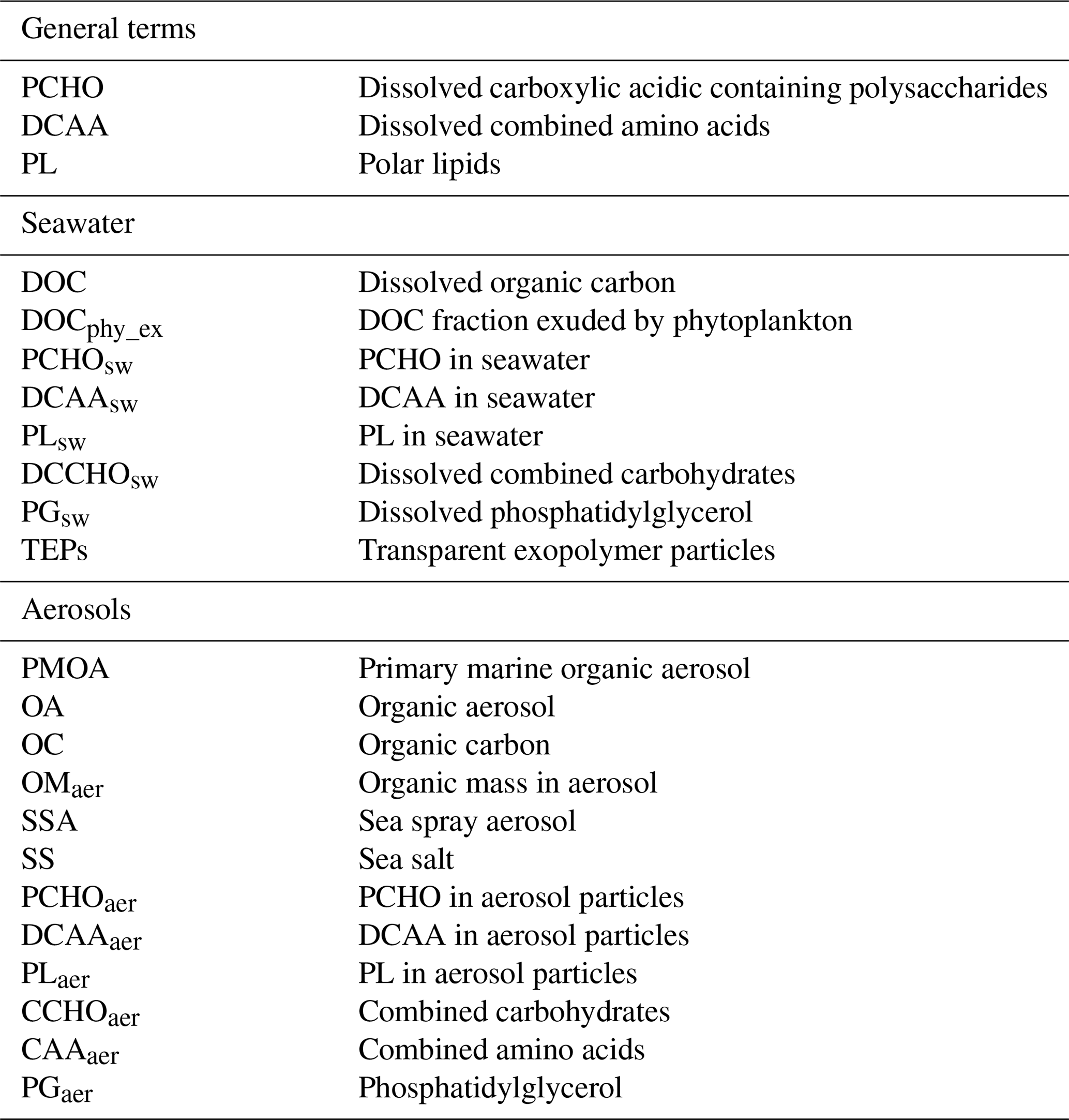
Table 2 List of abbreviations of the most relevant aerosol and seawater compounds considered in the present study.

2.3 Organic biomolecules in seawater

The main sources of dissolved organic matter in seawater are phytoplankton exudates, carbon release via cell lysis, zooplankton grazing on phytoplankton, and zooplankton excretion (Carlson, 2002). Additionally, DOC also significantly forms from particulate organic carbon biological degradation (Repeta, 2015). From these sources, phytoplankton carbon exudation is considered a significant part of phytoplankton primary production (Myklestad, 2000). The most abundant components measured in extracellular carbon released by phytoplankton are carbohydrates (mono-, oligo-, and polysaccharides), proteinogenic compounds (amino acids, proteins, and peptides), lipids (fatty acids and polar lipids such as phosphoglycerides and glycosylglycerides), and to a lesser degree organic acids (Lancelot, 1984; Yongmanitchai and Ward, 1993; Harwood and Guschina, 2009). Among these, polysaccharides, free and combined amino acids, and polar lipids represent the main biomolecule groups in the phytoplankton extracellular products (Parrish and Wangersky, 1987; Parrish et al., 1993, 1994; Obernosterer and Herndl, 1995; Engel et al., 2004; Arnosti et al., 2021).

These biomolecules can be measured both in seawater and in the aerosol phase (Kuznetsova et al., 2004; Zeppenfeld et al., 2020; Triesch et al., 2021b; van Pinxteren et al., 2023). In the present study we assume the aforementioned groups to be characterized by the biomolecules that form the majority of the phytoplankton extracellular carbon: dissolved carboxylic acidic containing polysaccharides (PCHO_sw), dissolved combined amino acids (DCAA_sw), and phospholipids and glycolipids as polar lipids (PL_sw) in seawater. The DOC fraction exuded by phytoplankton (DOC_{phy_ex}) is resolved in the FESOM2.1–REcoM3 model (Gürses et al., 2023), and we use it to derive the biomolecule groups. Based on these premises, we compute the ocean surface concentration of the biomolecules by apportioning the DOC_{phy_ex} into the contribution from each group:

$$\begin{array}{}\text{(4)}& {\mathrm{DOC}}_{\mathrm{phy}\mathrm{\_}\mathrm{ex}}={\mathrm{C}}_{{\mathrm{PCHO}}_{\mathrm{sw}}}+{\mathrm{C}}_{{\mathrm{PL}}_{\mathrm{sw}}}+{\mathrm{C}}_{{\mathrm{DCAA}}_{\mathrm{sw}}}+\mathrm{Res}.\end{array}$$

$C_{{\mathrm{PCHO}}_{\mathrm{sw}}}$, $C_{{\mathrm{PL}}_{\mathrm{sw}}}$, and $C_{{\mathrm{DCAA}}_{\mathrm{sw}}}$ refer to the surface ocean concentration of each group (seawater compartment in Fig. 1), while Res is the residual that will be attributed to compounds not included in the three main classes, with contributions ranging between 9 % and 38 % of DOC_{phy_ex} (Hellebust, 1965; Al-Hasan and Coughlan, 1976).

In the FESOM2.1–REcoM3 model, the DOC phytoplankton excretion rate (DOC_{phy_ex_rate}) describes the phytoplankton release per unit of time and is considered a source term in the semi-labile DOC (see Eqs. A42 and A55 in Gürses et al., 2023):

$$\begin{array}{}\text{(5)}& {\mathrm{DOC}}_{\mathrm{phy}\mathrm{\_}\mathrm{ex}\mathrm{\_}\mathrm{rate}}=({\mathit{ϵ}}_{\mathrm{phy}}^C{\mathrm{f}}_{\lim ,\mathrm{phy}}{\mathrm{PhyC}}_{\mathrm{phy}}+{\mathit{ϵ}}_{\mathrm{dia}}^C{\mathrm{f}}_{\lim ,\mathrm{dia}}{\mathrm{PhyC}}_{\mathrm{dia}}).\end{array}$$

PhyC refers to the phytoplankton carbon concentration, and the sub-indices “phy” and “dia” refer to small and diatom phytoplankton groups, respectively. ϵ is the excretion constant of organic carbon (d⁻¹), and f is a limiter function that downregulates the phytoplankton excretion when the nitrogen quota (qN : C) becomes too high.

To represent acidic dissolved polysaccharides in seawater (PCHO_sw) and TEPs, which are gel-like particles formed from PCHO_sw, Schartau et al. (2007) developed a formulation based on the extracellular production of organic carbon from phytoplankton and aggregation processes (see previous section). Simulated PCHO_sw accounts for approximately 63 % of exuded organic carbon by small phytoplankton and diatoms, representing the majority of the modelled DOC. According to laboratory studies, dissolved polysaccharides account for the highest fraction of exuded carbon by phytoplankton, and their contribution to the exuded carbon ranges from 47 % to 90 % (Myklestad, 1995; Biersmith and Benner, 1998; Hama and Yanagi, 2001). It is therefore assumed that

$$\begin{array}{}\text{(6)}& {\mathrm{C}}_{{\mathrm{PCHO}}_{\mathrm{sw}}}={\mathrm{PCHO}}_{\mathrm{sw}}{|}_{\text{FESOM–REcoM}}.\end{array}$$

Overall, lipid material in phytoplankton-exuded DOC ranges from 2.8 % to 10.3 % (Hellebust, 1965; Billmire and Aaronson, 1976). Considering that on average δ=5 % of the DOC_{phy_ex_rate} will be attributed to the extracellular PL_sw production rate ($S_{{\mathrm{PL}}_{\mathrm{sw}}}$), the ocean surface concentration can be approximated as $S_{{\mathrm{PL}}_{\mathrm{sw}}}$ multiplied by the lifetime (τ) of lipids in seawater after release:

$$\begin{array}{}\text{(7)}& {\mathrm{C}}_{{\mathrm{PL}}_{\mathrm{sw}}}=\mathit{\tau }{\mathrm{S}}_{{\mathrm{PL}}_{\mathrm{sw}}},\end{array}$$

with

$$\begin{array}{}\text{(8)}& {\mathrm{S}}_{{\mathrm{PL}}_{\mathrm{sw}}}=\mathit{\delta }{\mathrm{DOC}}_{\mathrm{phy}\mathrm{\_}\mathrm{ex}\mathrm{\_}\mathrm{rate}}.\end{array}$$

Lipids are short-lived compounds, whose turnover time is just a few days (Hopkinson et al., 2002; Karl and Björkman, 2015). Sensitivity studies, performed with typical turnover times of PL_sw between 4 and 10 d (Karl and Björkman, 2015), led to the best agreement with observation for turnover rates of 8 d.

$C_{{\mathrm{DCAA}}_{\mathrm{sw}}}$, on the other hand, was determined differently. Based on various concentration values measured in ambient seawater from different sites (see also the measurement description below), we calculated the ratio of observed dissolved combined carbohydrates (DCCHO_sw) and DCAA_sw (from 31 seawater samples). A median value of ratio = 0.3 ± 0.08 was obtained and is used here to compute DCAA_sw in the ocean based on PCHO_sw modelled concentration. Nevertheless, employing this method results in the estimated DCAA_sw encompassing both extracellular and intracellular carbon derived from phytoplankton. Consequently, the modelled concentrations reflect the aggregate of these two DCAA_sw formation mechanisms, as it is not feasible to differentiate the relative contribution of extracellular carbon released by phytoplankton based on observational data. Hence, in our approach, DCAA_sw will be the sole group for which the sources may include contributions beyond extracellular release by phytoplankton (C${}_{{\mathrm{DCAA}}_{\mathrm{sw}}}^{\prime }$).

$$\begin{array}{}\text{(9)}& {\mathrm{C}}_{{\mathrm{DCAA}}_{\mathrm{sw}}}^{\prime }=\mathrm{ratio}\cdot {\mathrm{C}}_{{\mathrm{PCHO}}_{\mathrm{sw}}}\end{array}$$

Considering that carbohydrates constitute a significant portion of semi-labile DOC, with turnover times ranging from months to years, the computed DCAA_sw will also contribute to this fraction. Therefore, the labile or refractory component of DCAA_sw is not included in the current study.

Values found in the literature indicate that extracellular amino acids represent 1.5 % to 7 % of exuded DOC (Myklestad et al., 1972; Mague et al., 1980; Granum et al., 2002). Presuming that extracellular DCAA_sw represents nearly 5 %, together with PCHO_sw and PL_sw, the biomolecules constitute approximately 73 % of exuded organic carbon by phytoplankton groups in FESOM2.1–REcoM3, where dissolved acidic polysaccharides account for the highest fraction. The residual 27 % may include other lipid-, polysaccharide-, and protein-like compounds, as well as organic acids or other unknown components.

2.4 Approximations of phytoplankton extracellular carbon release

The abundance of the biomolecule exuded by phytoplankton exhibits a significant temporal and spatial variability, primarily influenced by phytoplankton growth phase and nutrient availability (Myklestad, 2000). Other studies have demonstrated that the carbon exudation also differs among species (Hellebust, 1965; Wolter, 1982; Wetz and Wheeler, 2007). Furthermore, intense light conditions induce abrupt modifications in the extracellular release, with the proportion of carbon incorporated into cells remaining approximately constant in comparison to that exuded by phytoplankton, as documented by Mague et al. (1980).

During phytoplankton growth, extracellular carbon release is influenced by nutrient conditions. The exudation tends to be slightly higher for the rapidly growing than for the stationary phase (Myklestad et al., 1989). The exuded products differ for every case and phytoplankton species. For instance, higher levels of extracellular polysaccharides and free amino acid release were observed during phosphorus-limited conditions compared to balanced nutrient conditions (Obernosterer and Herndl, 1995). In contrast, whereas proteinogenic compounds and free amino acids decrease under nitrogen depletion (Granum et al., 2002), extracellular polysaccharides are significantly favoured (Myklestad, 1995).

Biogeochemical models often parameterize the phytoplankton carbon exudation by setting a constant phytoplankton biomass loss per day (Thornton, 2014). This fraction is set to 10 % for both phytoplankton groups in FESOM2.1–REcoM3 (Gürses et al., 2023). Moreover, the exuded carbon is regulated by a limiting factor as a measure of nutrient availability, which depends entirely on the carbon and nitrogen quota, and, lastly, it is independent of light conditions (see Eq. 5).

Furthermore, since simplifications are required for the global biogeochemistry model, diatoms and small phytoplankton do not distinguish the species within those groups. Therefore, the distinct characteristics of each phytoplankton culture, which exhibits an unequal distribution in seawater and extracellular carbon release levels (Granum et al., 2002), cannot be captured. Therefore, the values utilized in the present study to estimate the contribution of each biomolecule to the extracellular DOC released by phytoplankton in the ocean were either averaged across multiple laboratory studies or approximated, thus limiting them to known measured quantities in the literature (Hellebust, 1965; Billmire and Aaronson, 1976; Mague et al., 1980; Myklestad, 1995; Biersmith and Benner, 1998; Hama and Yanagi, 2001; Granum et al., 2002).

3 Global aerosol–climate simulations

3.1 The ECHAM6.3–HAM2.3 model

Aerosol–climate models represent aerosol emission, transport, wet and dry deposition, and direct and indirect radiative effects in the earth system. In this study, we used the model ECHAM6.3–HAM2.3 (Tegen et al., 2019), which combines the atmospheric general circulation model ECHAM6.3 (Stevens et al., 2013) with a spectral transform dynamical core (Lin and Rood, 1996) and the Hamburg Aerosol Module (HAM2.3) (Stier et al., 2005).

The aerosol microphysics module, HAM, is based on the M7 aerosol model (Vignati et al., 2004; Stier et al., 2005). The aerosol species considered in the model are sulfate (SO₄), organic carbon (OC), black carbon (BC), mineral dust (DU), and sea salt (SS). For OC, BC, and SO₄, emissions are initially prescribed from anthropogenic sources and biomass burning emission inventories and from volcanic eruptions. Wind-driven DU and SS emission fluxes from desert and the ocean, respectively, are calculated online in the model. Additionally, dimethyl sulfide (DMS) is emitted from the marine biosphere.

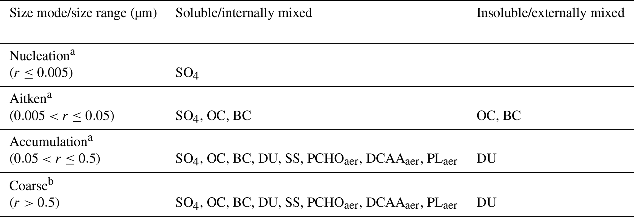
Aerosol species are divided into two groups of soluble and insoluble aerosol particles for a total of seven log-normal classes according to a predefined four-group aerosol size spectrum (Table 3). The aerosol mass and number concentration is predicted for each mode. The log-normal distribution depends on the aerosol number, median radius, and standard deviation. Modes exist as soluble or insoluble. All species in a soluble mode are considered to be internally mixed, meaning that every particle is actually a mixture of all the species within the mode.

The PMOA compounds are treated as separate tracers and included in the model as three new individual species (atmosphere compartment in Fig. 1) to the soluble accumulation and coarse modes (see Table 3). These organic groups do not contribute to but share the microphysical and optical particle properties of the OC tracer. Since the model does not represent sea spray emission for the Aiken mode, PMOA is initially emitted solely into the accumulation mode. Then, the particles grow by coagulation or condensation, increasing the mean geometric radii and eventually transitioning to a larger mode.

Table 3 Aerosol modes and compounds in HAM. r denotes the radius of the respective particle size range and σ the standard deviation.

^a σ=1.59. ^b σ=2.0.

HAM includes aerosol transformation processes such as the nucleation of sulfuric acid and water droplets, coagulation and condensation of sulfuric acid, and water uptake. In addition, deposition, aerosol interactions with clouds, and radiation are also accounted for. The updated version of HAM2.3 encompasses several improvements to the aerosol processes and emission (Tegen et al., 2019) as well as to aerosol–cloud interactions (Lohmann and Neubauer, 2018).

The two-moment cloud microphysics scheme in ECHAM6.3–HAM2.3 follows Lohmann et al. (2007) and Lohmann and Hoose (2009). It allows for in-cloud and below-cloud scavenging aerosol processes for liquid, ice, and mixed-phase clouds. The cloud droplet activation is based on the Köhler theory by Abdul‐Razzak and Ghan (2000). ECHAM6.3 has implemented a rapid radiative transfer model (PSrad/RRTMG) to represent the radiative interaction with aerosols and clouds (Pincus and Stevens, 2013).

3.2 Emissions of sea spray aerosol

Marine aerosols emission flux is calculated based on Eq. (2). where PMOA and SS make the total sea spray mass. Thus, the emitted PMOA mass flux of each biomolecule group (i) can be computed as

$$\begin{array}{}\text{(10)}& {\mathrm{PMOA}}_{\mathrm{mass}\mathrm{flux}}\left(i\right)={\displaystyle \frac{{\mathrm{SS}}_{\mathrm{mass}\mathrm{flux}}\cdot {\mathrm{OMF}}_i}{\mathrm{1}-{\mathrm{OMF}}_i}},\end{array}$$

where OMF refers to the organic mass fraction parameterized based on OCEANFILMS (Burrows et al., 2014), as previously described. SS_mass flux is the mass flux of sea salt emitted in ECHAM6.3–HAM2.3. The model includes a range of widely used sea salt emission schemes, including, among others, Guelle et al. (2001), Gong (2003), and Long et al. (2011). The default configuration is considered for the current study and follows Long et al. (2011) with sea surface temperature correction according to Sofiev et al. (2011). This combination showed the best agreement with observed surface sea salt aerosol concentration and particle size distribution across multiple marine sites in the model evaluation study by Tegen et al. (2019).

Following Burrows et al. (2022), we assume that PMOA is internally mixed and the number and fluxes added onto sea salt. The authors performed sensitivity studies with various combinations of the mixing state of PMOA with sea salt in the Energy Exascale Earth System Model (E3SM). Their findings indicate that the chosen configuration provided a better seasonal representation of organic mass and aerosol concentration compared to observations.

3.3 Experimental setup

The aerosol–climate model simulations are performed at T63 (approx. 1.875° × 1.875°) horizontal resolution with a total of 47 vertical levels, which resolves the atmosphere from the surface up to 0.01 hPa. The model is run in nudged mode with the re-analysis data from the European Centre for Medium-Range Weather Forecasts (ECMWF) known as ERA-Interim. Sea ice concentration (SIC, as the percentage of area covered by ice) and sea surface temperature (SST) monthly mean values from the Atmospheric Model Intercomparison Project (AMIP) (Taylor et al., 2000) are used as boundary conditions for the model experiments. The simulations cover a period of 10 years (2009–2019) in which aerosol measurements were available. A spin-up time of 4 months and an output frequency of 12 h were considered.

Two experiments, without and with simulated PMOA as a tracer in the model, were performed, hereafter referred to as SPMOAoff and SPMOAon, respectively. The SPMOAoff simulation only accounts for the fraction of sea salt in sea spray aerosol, whereas the SPMOAon utilizes the biomolecule ocean surface concentration as bottom boundary conditions to compute the marine organic aerosol fraction in addition to the sea salt. For consistency with the biogeochemistry-model-predicted sea ice, an adjustment of SIC and SST within the sea salt emission scheme is considered, intending to avoid ambiguities. To ensure comparability with previously published results of the aerosol–climate model (Tegen et al., 2019) and avoid re-tuning, the AMIP data are retained for the simulations. A mask is applied to determine when FESOM2.1–REcoM3 model SIC and SST values replace or modify AMIP data. Whenever ice-free (SIC < 10 %) conditions for the marine biogeochemistry model are satisfied, the AMIP SIC values are updated during runtime to 0 % and SST is replaced by that from FESOM2.1–REcoM3. Note that the mask only applies when the sea salt emission scheme is called, thus not affecting the rest of the globe.

4 Observations for model evaluation

In this section, we will discuss the measurement data selected for the model evaluation. We present the seawater sample data of measured marine compounds that are being compared with the concentration of marine biomolecules in the ocean. Likewise, we validate the offline-computed organic mass fraction and simulated aerosol concentration of each group with analogous compounds from observations. This species-wise evaluation will assess how well the models can represent the different biomolecules in seawater and the atmosphere. Nonetheless, the data are primarily accessible for specific locations and do not provide an overview of marine organics' abundance in remote oceanic areas. Thus, as the final dataset for model evaluation, in situ airborne organic aerosol concentration measurements with extensive coverage of most oceanic regions are used to provide a more thorough evaluation of PMOA.

4.1 Seawater samples and in situ ground-based measurements

Modelled estimates of ocean surface concentration of biomolecule and aerosol OMF and concentration (Fig. 1) are compared to bulk seawater samples and aerosol observations from various stations worldwide (Fig. 2). Table 5 summarizes the most relevant information of these marine and aerosol measurements. The comprehensive collection of observational data in this study was compiled considering similar sampling techniques and laboratory instruments to detect and measure the concentration of the organic compounds. Details on the compounds selected for the model evaluation are introduced in this section. Additionally, a brief description of the interpolation of model results for the comparison is presented.

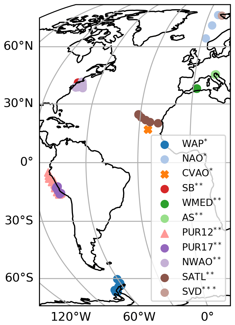
Figure 2 Station locations for seawater samples and marine aerosol measurements. The circles, triangles, and cross markers indicate the stations for which one, two, and three compounds were measured, respectively. The asterisks indicate the type of data available at each location: ^* – seawater and aerosol; ${}^{**}$ – only seawater; ${}^{***}$ – only aerosol. See Table 4 for the location abbreviations. The most relevant information regarding the data can be found in Table 5.

Seawater samples were collected between 10 cm and 3.5 m depth, often with a plastic or glass bottle to collect the water at a specific depth. For simplicity, only measurements from the open ocean without sea ice were included. Whereas the model mostly represents the biomolecule production from phytoplankton, the in situ measurements do not allow us to trace back the production mechanism of these groups. Hence, modelled quantities may represent a portion of the measured biomolecules. Although the measurements are not strictly comparable to the model results, they are good indicators to validate the modelled quantities.

We therefore selected analogous components for the model evaluation. Seawater measurements of dissolved combined carbohydrates (DCCHO_sw), dissolved combined amino acids (DCAA_sw), and dissolved phosphatidylglycerol (PG_sw) were chosen for comparison with modelled PCHO_sw, DCAA_sw, and PL_sw, respectively. DCAA_sw is considered to be approximately equal to the measured hydrolysable dissolved combined amino acids (DHAA). On the other hand, the selection of PG_sw, was based on the fact that phytoplankton extracellular lipids are essentially formed by phosphoglycerides and glycosylglycerides (Yongmanitchai and Ward, 1993; Guschina and Harwood, 2009). Moreover, the presence of this compound in seawater is often correlated to phytoplankton (Triesch et al., 2021b).

Additionally, aerosol data were carefully cleaned, including only those for which a correlation with marine biological activity has been reported. Aerosol samples were collected in filters exposed at heights between 4 and 50 m a.m.s.l. For the aerosols, we selected the same tracers that are linked to the marine amounts. Observations of combined carbohydrates (CCHO_aer), amino acids (CAA_aer), and PG_aer are available for comparison to the simulated aerosol concentration and organic fraction of PCHO_aer, DCAA_aer, and PL_aer, respectively (Table 5).

OMF for each group is available from OCEANFILMS. On the other hand, for the measurements, we derived OMF based on the observed marine aerosols and sea salt mass, which was estimated as a constant rate ($\mathrm{1}/\mathrm{0.3061}$) of sodium (Na⁺) concentration (Seinfeld and Pandis, 2006). Lastly, OM_aer is derived from the measured OC, considering a ratio of OM : OC = 2 of remote region aerosols following Turpin and Lim (2001). Nonetheless, this ratio may vary as aerosol particles age in the atmosphere and depending on the content of water-soluble organic material (Sciare et al., 2005; Facchini et al., 2008).

For the model evaluation, simulated results are interpolated to the observation sites using a cubic-triangular-based interpolator, a suitable method to detect and account for gradients in the data. Note that we use monthly ocean values, which do not capture the spatial and temporal variability in marine biogeochemistry within a month (e.g. CVAO seawater samples in Triesch et al., 2021b). This can affect cases where the quantity of samples is limited and restricted to a single location, such as CVAO, where the interpolated ocean concentrations remain nearly identical. Nevertheless, a comprehensive examination of the daily modelled PCHO_sw against observations (not shown) for the summer of 2017 revealed an overall lower agreement with water samples than when utilizing monthly mean values.

For the aerosol comparison, we interpolated the near-surface model vertical level aerosol concentration to the coordinates of the stations. Most stations are land-based, except for NAO and WAP, in which aerosols were sampled on board of a ship. For these cases, we interpolated the simulated values for the ship trajectories and averaged over a starting and ending point in accordance with observations. For Svalbard, filters were exposed for at least 6 d. Hence, interpolated model values were averaged over these period for the comparison with observations.

Table 4 List of abbreviations and coordinates of the locations of the measurement campaigns and observational stations used for the model evaluation.

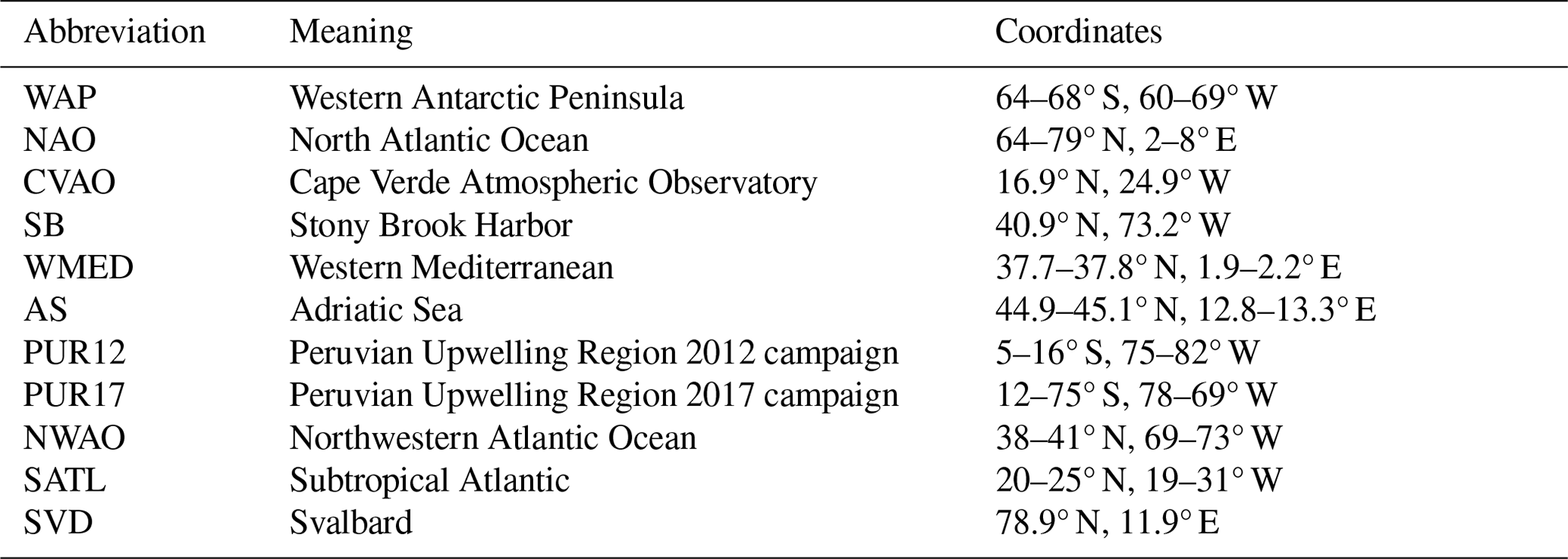
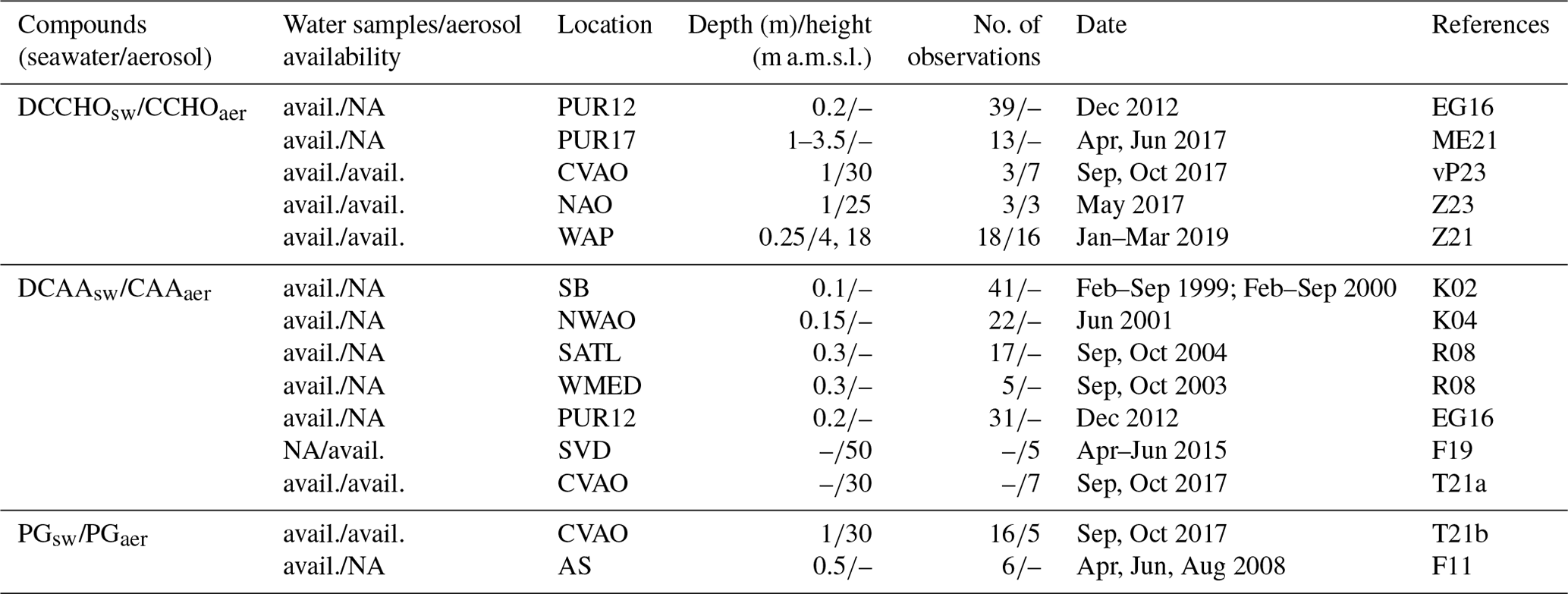
Table 5 Bulk water samples and aerosol measurements selected for the comparison with modelled biomolecule and aerosol tracers. Seawater sampling techniques employed during each campaign of each molecule group are the same. The measurement techniques are high-performance anion exchange chromatography coupled with pulsed amperometric detection (HPAEC-PAD) for quantifying DCCHO_sw, high-performance liquid chromatography (HPLC) for DCAA_sw, and thin-layer chromatography with the flame ionization detection (TLC/FID) for PG_sw. See Tables 2 and 4 for the compound and location abbreviations, respectively. References abbreviations: EG16 – Engel and Galgani (2016); vP23 – van Pinxteren et al. (2023); Z23 – Zeppenfeld et al. (2023); Z21 – Zeppenfeld et al. (2021); ME21 – Maßmig and Engel (2021); K02 – Kuznetsova and Lee (2002); K04 – Kuznetsova et al. (2004); R08 – Reinthaler et al. (2008); F19 – Feltracco et al. (2019); T21a – Triesch et al. (2021a); T21b – Triesch et al. (2021b); F11 – Frka et al. (2011). NA represents not available.

4.2 Aircraft observations of organic aerosols

To provide an overview of the model's capability to represent PMOA in remote oceanic regions where ground-based measurements are not available, we compare the simulated PMOA concentrations with aircraft observations over the ocean regions that are least affected by organic carbon from non-marine sources. Mass concentrations of organic aerosols (OAs) from the Atmospheric Tomography (ATom, https://espoarchive.nasa.gov/archive/browse/atom, last access: 1 August 2024) campaigns of the US National Aeronautics and Space Administration (NASA) are used for the comparison to the aerosol model results. Information regarding the different instruments on board the aircraft, measuring aerosol quantities, can be found at the official website. The aircraft flew mostly over open-ocean areas and within the Arctic region. The data are available at a temporal resolution of approximately 15 min.

Some studies analysing ATom data indicate that PMOA could significantly contribute in remote oceanic regions to the OA (Pai et al., 2020). Following Pai et al. (2020), we selected the near-surface levels from ATom data (heights under 1 km) limiting the comparison to the marine boundary layer, in which marine local sources should predominate. In an attempt to exclude organic aerosol from anthropogenic and biomass burning sources that mostly influence the Northern Hemisphere, we imposed a threshold to OA values and excluded those over 0.2 µg m⁻³ (measured at standard temperature and pressure conditions: 273 K, 1 atm) as in the regime's classification by Pai et al. (2020). Figure 3a shows the data grouped by months after applying the aforementioned conditions. Any data collected inland, where primary marine aerosols have no impact, were excluded, reducing the dataset to the open-ocean or near-coastal regions. The majority of the data was measured in October 2017, followed by February of the same year and May 2018 (with a sample size of 64, 40, and 30 observations, respectively). The remaining cases comprise fewer than 12 observations. Since some of the flight trajectories overlap, the Fig. 3a does not visually represent the actual number of samples for some cases.

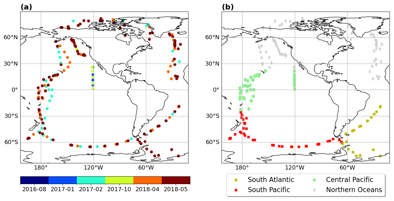
Figure 3 (a) Airborne organic aerosol particles grouped by days for diameters smaller than 1 µm, altitudes below 1 km, and concentrations smaller than 0.2 µg s m⁻³. (b) Colour-coded regions selected for the model evaluation. The northern ocean region potentially most influenced by long-range-transported aerosols is represented here for reference (in light gray) but excluded from the model evaluation analysis.

To distinguish pristine regions that are most likely dominated by PMOA from those that are more anthropogenically influenced or more polluted, we only selected the flight legs for the model evaluation as shown in Fig. 3b. Northern Hemisphere aerosols, which are predominantly dominated by anthropogenic sources, biomass burning, and natural fires and would therefore mask the weaker signal of the PMOA, are thus excluded from the comparison (light gray locations in Fig. 3b).

For the evaluation of model results, the hybrid model vertical levels were transformed into pressure levels and linearly interpolated to the flight horizontal coordinates and altitude where the aerosols were sampled. Since the model output is only 12-hourly, we spatially interpolated the flight points, which laid within this 12 h range. This means that all flight coordinates between 00:00 (12:00) UTC and 12:00 UTC (00:00 UTC of next day) of a certain day are interpolated to the model output corresponding to the same day at 12:00 UTC (00:00 UTC of next day). Then, we derived daily averages of observational and modelled values and calculated the correlation coefficient and model bias for the whole dataset, accordingly. Additionally, model results were converted to standard conditions of temperature and pressure to meet the conditions, at which the ATom aircraft samples were measured.

5 Results and discussion

5.1 Geographical distribution of modelled biomolecules

Based on the FESOM2.1–REcoM3 model data and the calculations in Sect. 2.3, the three key marine biomolecules at the sea surface have an average spatial distribution as shown in Fig. 4a–c. In addition, Fig. 4d–f present the aerosol organic mass fraction (OMF) calculated with the OCEANFILMS scheme as considered in this study in an offline mode with the simulated ocean surface concentration as input data.

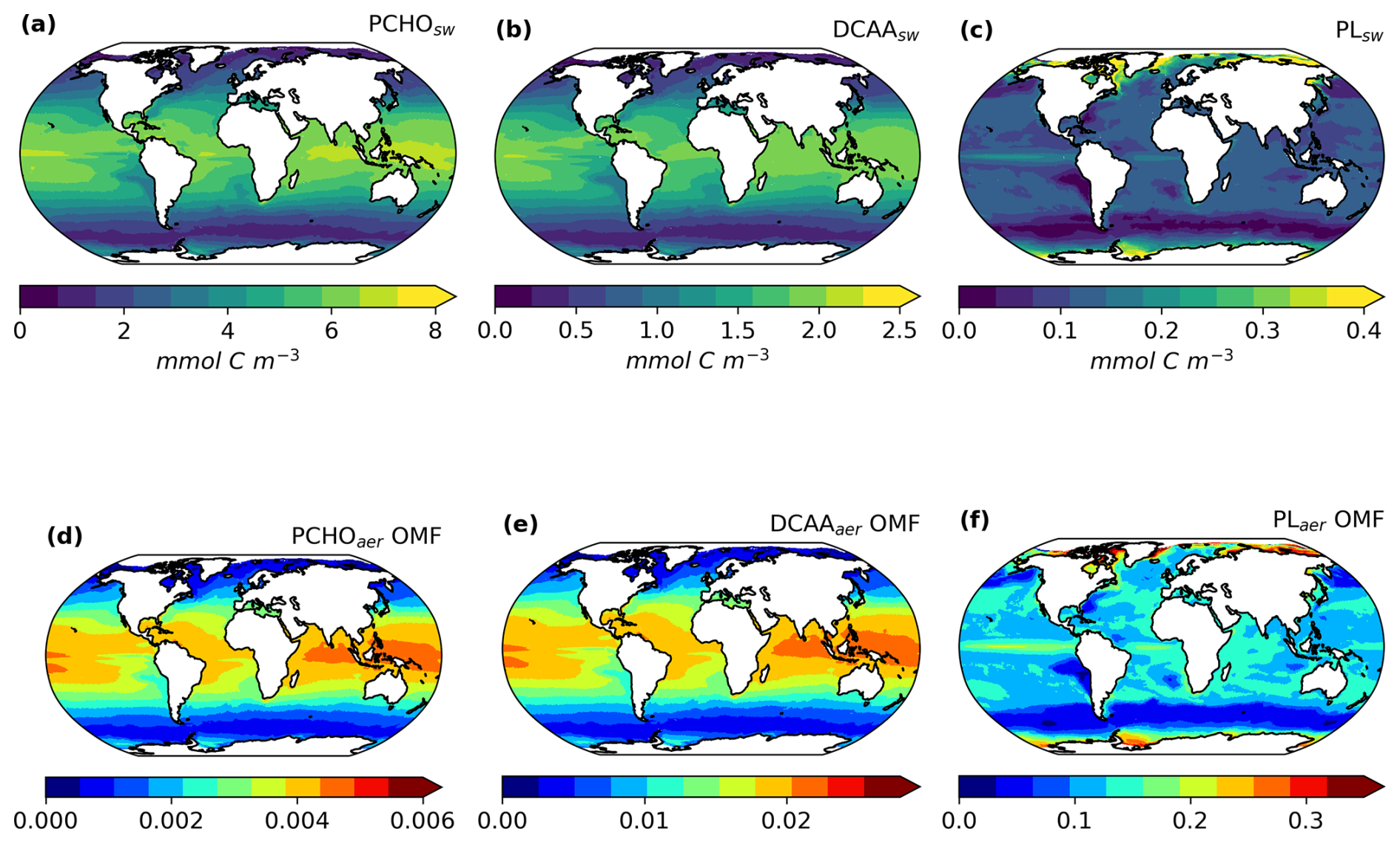
Figure 4 Maps of global-averaged (a–c) ocean carbon concentration of PCHO_sw, DCAA_sw, and PL_sw and (d–f) offline-computed OMF of PCHO_aer, DCAA_aer, and PL_aer as a multiannual mean for the period 1990–2019 for sea-ice-free conditions (SIC < 10 %).

5.1.1 Sea surface concentration of biomolecules

The global distribution of marine biomolecules exhibits distinct patterns for the semi-labile groups PCHO_sw and DCAA_sw, in contrast to the labile PL_sw group, due to their resistance to rapid microbial utilization. PCHO_sw, as the main extracellular product of phytoplankton, has a maximum concentration of up to 8.4 mmol C m⁻³. DCAA_sw and PL_sw have values as high as 2.5 and 1.28 mmol C m⁻³, respectively (see Fig. 4a, b).

PCHO_sw and DCAA_sw show persistently high concentrations over tropical waters (Fig. 4a, b). This is linked to the strong stratification that prevents deep vertical mixing and remineralization. In addition, we also associate these patterns with the carbon-overflow hypothesis (Engel et al., 2004, 2020), in which the carbon exudation increases under nutrient-limiting conditions. In FESOM2.1–REcoM3, nitrogen is indeed the most limiting factor of small phytoplankton in the vast areas of tropical and subtropical waters (Schourup-Kristensen et al., 2014; Gürses et al., 2023). For polar regions, on the other hand, the model results have the lowest values during polar night. In the bloom period during northern hemispheric spring, the PCHO_sw and DCAA_sw concentrations in the Arctic rise to values slightly higher than 8 and 2.5 mmol C m⁻³, respectively (see Fig. B1d–e). For the Southern Ocean, however, the maximum tends to be lower, at 5.3 mmol C m⁻³ for PCHO_sw and 1.6 mmol C m⁻³ for DCAA_sw (see Fig. B1a, b). The distinction can be attributed, among other factors, to the presence of significant river mouths in the Arctic, which serve as a significant source of nutrients for the polar waters that are not present in the Southern Ocean.

The greatest contributions of PL_sw (Fig. 4c) are found in the equatorial upwelling region and polar waters (see Fig. B1). Lower values predominate in the subtropical gyres where carbon exudation is solely dominated by the small phytoplankton group. In contrast to the other biomolecules, the values are lowest in the tropics, while higher contributions are found in the Arctic and Antarctic waters during the bloom period (Fig. B1c, j). Lastly, the low quantities simulated in the subtropical Pacific off the west coast of South America are common for all biomolecules. For this area, the dissolved inorganic nitrogen in the FESOM2.1–REcoM3 model has been excessively high compared to observations (Gürses et al., 2023). Additionally, the high nitrogen concentration also observed in the Southern Ocean could explain the low phytoplankton carbon exudation in this region. For this case, the intracellular nitrogen quota of small phytoplankton is high. As a consequence, the limiting function in Eq. (5) downregulates the carbon excretion. Therefore, the modelled carbon phytoplankton exudation is minimal given the elevated availability of nitrogen in these areas.

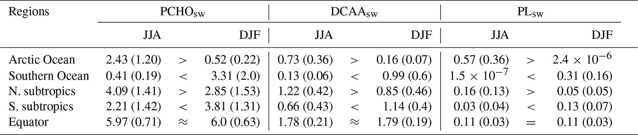
In addition to the spatial patterns, the seasonality of biomolecules in the ocean was also analysed by region (Table 6). All quantities are highest during hemispheric summer for the poles and subtropics (Fig. B1). For June–July–August, the total concentration of all biomolecules is on average 3.72 ± 1.74 and 0.55 ± 0.23 mmol C m⁻³ for the Arctic and Southern Ocean, respectively. During December–January–February the concentration increases in the southern region (4.61 ± 2.7 mmol C m⁻³) and declines in the Arctic seas 0.68 ± 0.29 mmol C m⁻³). Whereas the concentrations of PCHO_sw and DCAA_sw drop by about 80 % during the polar night, PL_sw falls to almost zero (Table 6). The amplitude between seasons is nearly twice smaller for the subtropics compared to the poles. Nevertheless, total quantities are larger for subtropical waters with values of 5.48 ± 1.81 mmol C m⁻³ (3.75 ± 2.02 mmol C m⁻³) and 5.07 ± 1.73 mmol C m⁻³ (2.9 ± 1.9 mmol C m⁻³) during summer (winter) for the northern and southern high latitudes, respectively. In contrast, seasonal patterns diminish towards the Equator (7.9 mmol C m⁻³), where they are absent due to the intense solar radiation being a limiting factor rather than nutrient depletion (Fig. B1). To our knowledge, there have been scarcely any studies on the surface concentration of marine organic compounds relevant for aerosols and none on the modelling of the carbon groups presented here. Two examples that closely resemble this work are the studies conducted by Ogunro et al. (2015) and Burrows et al. (2014). Among other groups and bio-indicators of ocean marine biological activity, Ogunro et al. (2015) presented the abundance of polysaccharide-, protein-, and lipid-like mixtures. Burrows et al. (2014) based their OCEANFILMS calculations on the macromolecule quantities, similarly derived from the same biogeochemistry model as in Ogunro et al. (2015). These two research studies assumed that the primary source of total DOC was cell lysis, and based on this assumption, they calculated the concentration of the macromolecular groups at the sea surface. Their computed quantities encompass a broader group than those examined in our study. Polysaccharides were assumed to be equal to the semi-labile dissolved organic carbon pool from a biogeochemical model (Ogunro et al., 2015; Burrows et al., 2014), which is equivalent to the DOC_{phy_ex} from FESOM2.1–REcoM3 in our study. With this assumption, other potential sources of polysaccharides are included, leading to higher values than in this work (up to 10-fold) and slightly different geographical distribution. Nonetheless, similar to our results, the abundance of proteins and polysaccharides is more pronounced in lower-productivity waters compared to high-productivity regions (Burrows et al., 2014). As in our case, Burrows et al. (2014) assumed that the protein-like group is composed of a fraction of polysaccharides. Consequently, proteins have the same global distribution and seasonal characteristics as polysaccharides. Finally, the lipid-like mixture in Ogunro et al. (2015) also represents a larger group. In addition, the calculations to estimate this macromolecule include the zooplankton levels and the rate of phytoplankton disruption by zooplankton grazing. As a consequence, higher values for the concentration at the sea surface are found for this group (about 5-fold) compared to PL_sw in the present study. Nonetheless, the ocean distribution of PL_sw agrees reasonably well with that presented by Burrows et al. (2014). Regardless of the considerations assumed to compute the biomolecules in the ocean, our approach adequately depicts the abundance of the biomolecules in the ocean that are relevant for the aerosols. The seasonal patterns modelled here also agree with those in Burrows et al. (2014), and the polysaccharide group is most frequently represented, followed by amino acids and lipids.

Table 6 Carbon concentration of marine biomolecules for December–January–February (DJF) and June–July–August (JJA) as a multiannual monthly mean for the period 1990–2019 averaged over the polar regions (Arctic Ocean 60–90° N, Southern Ocean 60–90° S), northern and southern subtropics (23–60° N and 23–60° S), and Equator (23° N–23° S). Values are in millimoles carbon per cubic metre (mmol C m⁻³). In parentheses, the multi-seasonal and regional standard deviation.

5.2 Aerosol organic mass fraction

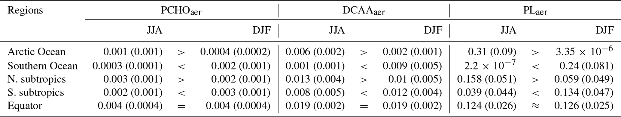
The organic mass fraction in aerosols depends on the distribution of marine biomolecule concentration in the ocean (Fig. 4d–f). In contrast to the abundance of organic groups in seawater, the OMF of polar lipids is significantly higher than that of the other groups during the hemispheric summer (see Fig. B2). Contributions can be as high as 0.44. In contrast, for PCHO_aer and DCAA_aer, OMF values are low, reaching a maximum of 0.004 and 0.02, respectively (Fig. 4d–f). The disproportional enrichment observed in the aerosol phase is explained by the aforementioned characteristics of the surface affinity of the main biomolecule groups in seawater (Sect. 2.1). Lipids are highly active surfactants whose surface affinity favours their transfer to the aerosol phase. Consequently, the OMF of PL_aer is 2 to 3 orders of magnitude greater than that of PCHO_aer and DCAA_aer (Fig. 4d, e), and these high values persist globally.

Among the biomolecules, PL_aer OMF is the group showing the most pronounced seasonal patterns with values generally decreasing towards the Equator during the hemispheric summer (Table 7 and Fig. B2c, f, j, m). PCHO_aer and DCAA_aer OMF values, on the other hand, remain uniform across seasons for subtropical and equatorial areas (see Fig. B2). For the polar regions, the abundance of all organic groups in aerosols has a clear seasonality, with strong changes for the PL_aer group (see Fig. B2d–j). These seasonal characteristics are caused by an increase in marine primary production as light limitation decreases at the end of the winter. With melting sea ice, light is available in ice-free areas or passes through the thin ice triggering the photosynthesis of phytoplankton. Once nutrients present in seawater are consumed and the polar night sets in, the biological productivity and atmospheric contribution of marine organics are significantly diminished, especially for PL_aer.

As expected, the responses of the various groups mirror those in Burrows et al. (2014). Nevertheless, based on the fundamental distinctions among the organic classes analysed, between the two studies, our OMF values are comparatively smaller yet still comparable to their findings.

Table 7 OMF of biomolecule groups in aerosols for the same regions and seasons in Table 6.

5.3 Evaluation of modelled biomolecules at the ocean surface

A comparison of simulated biomolecule concentrations with their measured counterparts in seawater is presented in this section. Each group is analysed against its analogous group from observations (see Sect. 4.1), supported by a discussion of the factors associated with model uncertainties. Figure 5 shows the ocean concentration of modelled and observed quantities for the locations in Fig. 2 for which ocean measurements were available (Table 5). Note that modelled PCHO_sw and semi-labile DCAA_sw represent a fraction of measured DCCHO_sw and DCAA_sw, whereas observed PG_sw forms part of the PL_sw group.

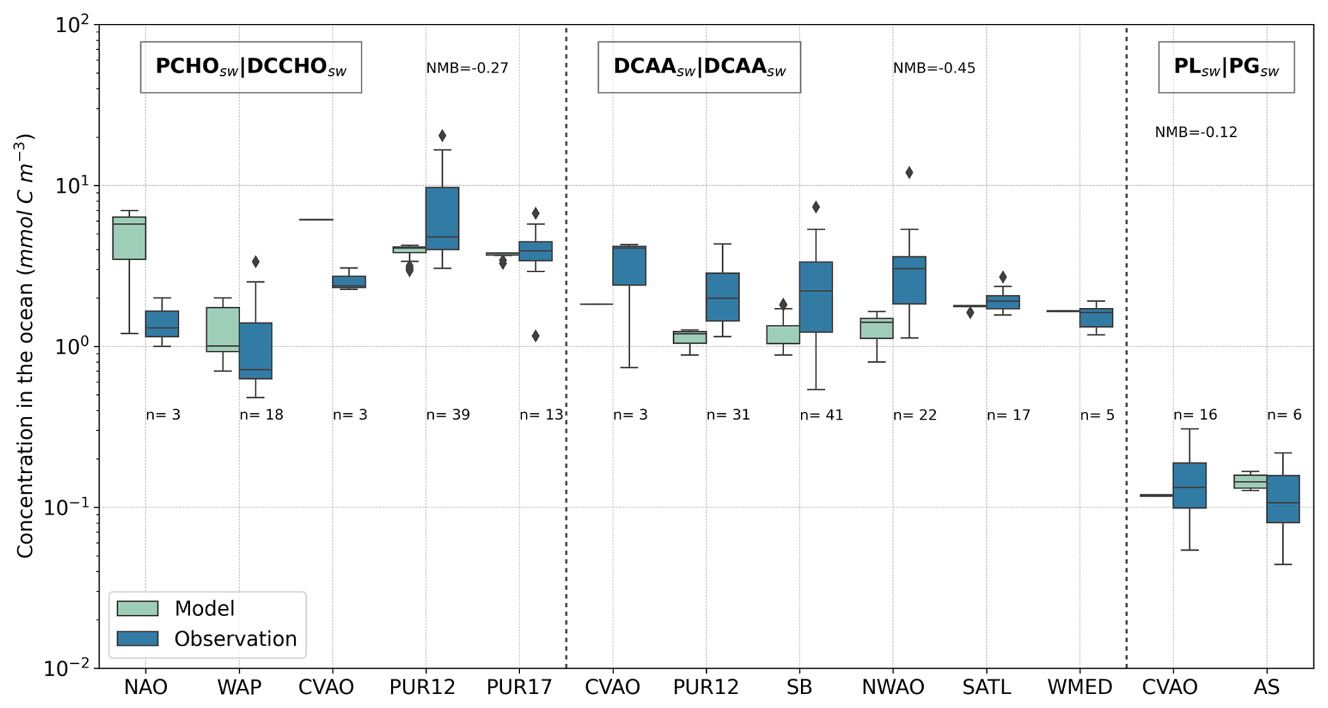
Figure 5 Box plot of carbon concentration in seawater of modelled PCHO_sw, DCAA_sw, and PL_sw and measured DCCHO_sw, DCAA_sw, and PG_sw for the locations in Fig. 2 (see also Tables 2 and 4 for the compounds and location abbreviations, respectively). Blue boxes represent the bulk water samples (Table 5), and coral boxes are the modelled biomolecule concentration interpolated to the coordinates where the water samples were collected. Normalized mean bias (NMB) is included for each group; number of observations (n) is included for all sites. The formula to calculate NMB may be found in Table A1.

5.3.1 Carbohydrates

The model (coral boxes in Fig. 5) can capture most of the regional variations seen in observations (blue boxes in Fig. 5). Quantities tend to be higher for the North Atlantic Ocean (NAO) compared to the Western Antarctica Peninsula (WAP). The lowest PCHO_sw concentration occurs at the southern station. This may be attributable to nutrient iron limitation in the Antarctic region (Gürses et al., 2023). Interestingly, the variability for WAP is better represented, although at a higher value than observations. Greater quantities are found at PUR12 and PUR17, where nutrients are transported from the seabed to the surface. Here, the modelled PCHO_sw concentration is in good agreement with observed DCCHO_sw, with a modelled median of 4.1 ± 0.39 and 3.8 ± 0.16 mmol C m⁻³ for PUR12 and PUR17, respectively. The lowest normalized mean bias (NMB) is detected for PUR17 (−0.08), whereas values are slightly overestimated for WAP (NMB =0.14) and underestimated for PUR12 (NMB $=-\mathrm{0.43}$).

The significant variability observed in PUR12 is not adequately captured by the model. The sampling depth may provide an explanation for this. The quantities would likely be greater for PUR12 if the water samples had been collected at 20 cm depth, in contrast to 1–3 m for PUR17. Maßmig and Engel (2021) found that concentrations of DCCHO and DCAA decrease with depth in this region. Note that FESOM2.1–REcoM3 vertical resolution is coarser and cannot resolve the processes within the SML solely including an average of the upper 5 m depth. Additionally, the model data used are a volume-weighted mean over the upper 30 m, and it is unlikely that subsurface water biomolecule abundances are accurately represented. Nonetheless, our results indicate that the modelled surface carbon concentrations of the biomolecules are in reasonably good agreement with the observations.

On the other hand, the modelled concentrations are about 4 times higher than the measurements for NAO (5.75 ± 2.48 mmol C m⁻³) and 2.5 times higher for CVAO (6.12 ± 0.01 mmol C m⁻³). NMB values for these locations are 2.24 and 1.38 for the northern and tropical sites, respectively. For these sites, the sampling size is relatively small (n=3) and the observations may not fully represent DCCHO_sw in the region. Nevertheless, the overestimation by the model could be explained by the carbon-overflow hypothesis (Engel et al., 2004, 2020), which states that carbon exudation is increased under nitrogen-limiting conditions. Moreover, bacteria are abundant in oligotrophic provinces like at CVAO and likely consume DOC, a process that is not explicitly represented in FESOM2.1–REcoM3 (Gürses et al., 2023).

In addition to the factors mentioned, we also link the overestimation in polar regions to the fixed fraction of exuded DOC that is generalized to all phytoplankton growth phases. Phytoplankton acidic polysaccharide excretion tends to be stronger during the post-bloom period compared to the phytoplankton growth phase. The amount of PCHO_sw exuded could be half of that currently used in the model representative of the post-bloom phase (Schartau et al., 2007).

5.3.2 Amino acids

For DCAA, the computed quantities are within the same range for all stations. Western Mediterranean (WMED) and subtropical Atlantic (SATL) are properly represented with median values close to observations (1.66 ± 0.01 and 1.78 ± 0.05 mmol C m⁻³, respectively) and a low model bias (NMB = 0.07 and −0.09, respectively). The oligotrophic sites show significantly less variability during the sampling period (September to October). However, they also have fewer data samples compared to other stations. Pertaining to the other locations, the estimated concentrations are confined to the lower quartile of the observations. The measured levels for PUR12, Stony Brook (SB), and the northwest Atlantic Ocean site (NWAO) are closely aligned. Among them, Stony Brook has the widest range in the sampled DCAA_sw. The higher variability is attributed to a substantial number of year-round measurements conducted at this location. For these subtropical sites, the variability is also apparent in the modelled DCAA_sw; however, it is not properly captured. The normalized model bias ranges between −0.6 and −0.49 for these stations, indicating an underestimation of the observed values. Nonetheless, apparent regional patterns are also found in the simulated biomolecules. For example, as for the observations, CVAO has the largest values and median concentrations of modelled DCAA_sw. Similarly, for NWAO (1.4 ± 0.28 mmol C m⁻³) DCAA_sw tends to be higher than for PUR12 (1.2 ± 0.12 mmol C m⁻³) and SB (1.04 ± 0.29 mmol C m⁻³).

The differences between the modelled and measured values are determined primarily by the approach used to calculate DCAA_sw. This biomolecule group was derived from the PCHO_sw concentration. Hence, detailed processes relevant for the production of amino acids in seawater are not represented here. Furthermore, as for carbohydrates, the concentrations of DCAA_sw tend to be greater near the surface (Maßmig and Engel, 2021). Therefore, the underestimations found for most cases could also be determined by the subsurface sampling depth, which was a maximum of 30 cm. Despite this, the modelled quantities agree reasonably well with the observed DCAA_sw.

5.3.3 Polar lipids

The observed PG_sw concentrations for the Adriatic Sea (AS) are slightly lower than for CVAO. In contrast, our results show higher concentrations for AS (0.14 ± 0.02 mmol C m⁻³) than for CVAO (0.12 mmol C m⁻³). Note that PG_sw may not fully represent all polar lipids in seawater. Nevertheless, the model values are in good agreement with the observed PG_sw, with the lowest model biases (NMB $=-\mathrm{0.12}$) compared to the other groups.

The observations indicate that the presence of the PG_sw group exhibits a strong correlation with the presence of phytoplankton (Triesch et al., 2021b). Therefore, the model estimates are closely aligned with the observed fraction of lipids produced by phytoplankton excretion. Nevertheless, the model cannot reproduce the variability for the tropical station. The monthly median values for this case remain within the same range (0.11 ± 0.03 mmol C m⁻³ in September and 0.15 ± 0.1 mmol C m⁻³ in October); however, there are notable inter-month changes that cannot be captured by the monthly means of the model.

Despite the fact that each biomolecule is analysed against broader measured groups in the ocean, this comparison serves as an indication of how effectively the modelled biomolecules are represented in terms of magnitude and geographic distribution.

In summary, model uncertainties depend on the considerations used to compute biomolecules, in which we neglected processes involved in their production or consumption. Additionally, the temporal and spatial resolution of the model is a source of uncertainty. Firstly, the monthly model values cannot represent changes within the same month (e.g. PUR12 and CVAO). Therefore, in certain instances, minor variations within a month may not be discernible, resulting in relatively homogeneous values and minimal standard deviations for the modelled quantities, such as CVAO, SATL, and WMED. Secondly, a common feature for tropics and subtropics is the coarser resolution of the non-uniform FESOM2.1–REcoM3 model mesh (Schourup-Kristensen et al., 2018) which could, to some extent, decrease the model accuracy for those regions. Lastly, the averaged values over the first 30 m of the model output agree better with observed biomolecule groups when the sampling depth was 1 m or deeper. Furthermore, for some stations (e.g. CVAO) the number of water samples was small, often within the same month, and may not be statistically representative of the existent variable conditions of the biomolecules for the region.

Regardless of the model biases, the calculated quantities lay within the same order of magnitude compared to observations for all cases. The different abundances of biomolecule groups in the ocean are well captured. The lipid group is the least abundant, with a concentration at least 1 order of magnitude lower than that of carbohydrates and amino acids.

6 Global atmospheric simulations of PMOA

We have already discussed in detail the geographical distribution and seasonality of marine biomolecules. Their concentrations at the sea surface serve as boundary conditions for the aerosol model. The results of the global aerosol simulations are presented in the following sections. We included an analysis of global mean burden and emission mass flux in the context of previous PMOA modelling studies. Furthermore, a comprehensive model evaluation against aerosol measurements is presented.

6.1 Emission and transport characteristics

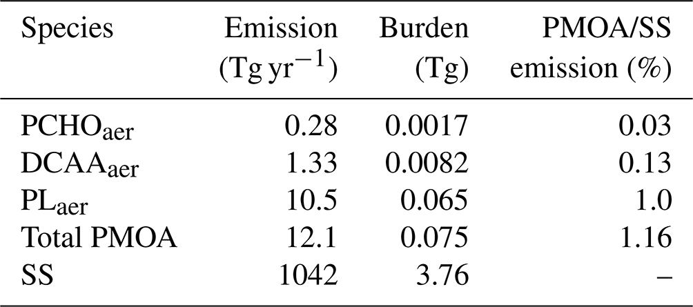
The global mean emission and burden values of marine aerosol are summarized in Table 8 for all organic species and sea salt. In addition, PMOA quantities are given as totals of the marine organic aerosol groups. Global emissions and burden are mainly governed by PL_aer, representing about 1 % of the sea salt emission by mass. This group accounts for 86.7 % of PMOA, whereas PCHO_aer and DCAA_aer make up 2.3 % and 11 %, respectively. Since hygroscopicity parameters are assumed to be identical and all groups are emitted into the same aerosol mode of the HAM model, their contribution to the total burden remains relatively unchanged compared to the emissions.

The global emission values modelled in this study total 12.1 Tg yr⁻¹, which is within the range of previous studies that vary between 9 and 27 Tg yr⁻¹ (Meskhidze et al., 2011; Huang et al., 2018; Zhao et al., 2021). Similarly, a total mean burden of 0.075 Tg agrees with other studies, ranging from 0.048 to 0.097 Tg (Huang et al., 2018; Zhao et al., 2021; Burrows et al., 2022). Given the similarities in terms of model configuration, our values are closer to the results by Huang et al. (2018) despite the chl-a approach used in their study to compute PMOA. This indicates that the driving aerosol–climate model has a greater influence on the final computed PMOA emissions than the specific representation of marine organics. There is also likely attributable to the sea salt emission scheme employed within the model. Therefore, the ratio of PMOA to SS emission mass fluxes varies across studies, and in our case, it is larger (1.16 %, Table 8) than the ratios presented by Zhao et al. (2021) (0.67 %) and Meskhidze et al. (2011) (0.7 %).

The PMOA representation depends directly on wind speed (Gantt et al., 2011) or on a sea salt emission source function (Meskhidze et al., 2011; Zhao et al., 2021). Sea salt emissions are typically parameterized in relation to the 10 m wind speed power law and/or as a function of the sea surface temperature (Gong, 2003; Mårtensson et al., 2003; Long et al., 2011).

For a more in-depth understanding of the driving processes that control the emission, dispersion, and removal of marine organic aerosol, we examine the connection among multiple model variables. In our study, the PMOA surface emission fluxes (Fig. 6a) are mainly driven by surface wind. Their geographic distribution is strongly linked to that of sea salt. Nonetheless, in regions where sea salt emissions are relatively low (e.g. high latitudes over 60° of each hemisphere during summer), the distribution of marine organic aerosol is primarily dominated by the elevated biological activity during the bloom period. The strongest emission fluxes occur in the Indian Ocean followed by the North Pacific Ocean with maximum values of 7.82 and 4.88 ng m⁻² s⁻¹, respectively. The total mean emission flux for North Pacific waters tends to be 35 % larger than that for the North Atlantic. For the Southern Ocean, the total emission flux is low (0.14 Tg yr⁻¹), and values in neighbouring waters (South Atlantic, Indian, and Pacific oceans) are 7- to 23-fold higher.

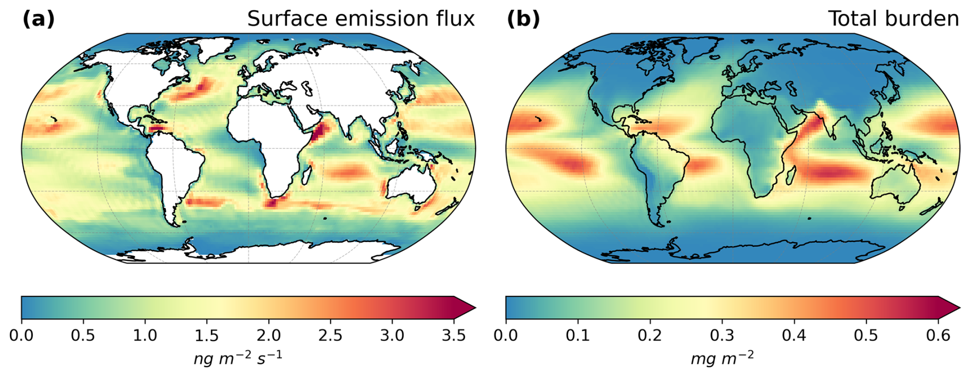
Figure 6 Maps of PMOA means of (a) global surface emission mass flux and (b) total burden for the simulated ECHAM6.3–HAM2.3 period 2009–2019.

Once emitted, aerosols are advected and driven by the general atmospheric circulation. If they are not scavenged by wet deposition mechanisms, they will remain longer in the atmosphere. These processes regulate the total aerosol burden, which also peaks in regions with lower surface emissions (e.g. equatorial Pacific). In regions with high biological productivity, such as the North Atlantic and North Pacific oceans, the main removal mechanism of PMOA is wet deposition, likely due to large-scale precipitation. In both hemispheres, the transport accumulates the aerosol towards the Equator. In addition, the marine aerosols are advected inland, with a significant incidence in coastal regions and over continental regions (e.g. widespread contributions in South America and Australia). Quantities could be as high as 0.3 mg m⁻² and even stronger in the northwest of India and the Horn of Africa.

The burden exhibits a similar behaviour to the emission flux, regarding the occurrence in the oceans. Quantities for the Pacific Ocean (0.017 to 0.019 Tg) remain larger than for the Atlantic Ocean (under 0.0072 Tg). Unlike the Atlantic, the difference in the burden between North Pacific and South Pacific increases and is reversed when compared to the emissions. Such differences, in which the highest emissions do not coincide with greater burdens, are caused by the transformation and transport processes that the aerosols undergo in the model. In the Southern Ocean, for instance, the total burden is at 0.0003 Tg about 50-fold lower than in the Indian Ocean. Lastly, the emissions and burden in the Arctic are among the lowest by approximately 2 and 3 orders of magnitude in comparison to the North Atlantic waters.

Table 8 Global mean emission flux and burden of marine species and sea salt. Note that emissions of PMOA are confined to the accumulation mode, whereas SS emissions occur in both the accumulation and coarse modes.

6.2 Species-wise evaluation

In this section, we present the results of a comprehensive analysis of species-resolved offline-computed OMF and ECHAM6.3–HAM2.3 aerosol concentrations against observations. The modelled aerosol organic mass fraction is the result of applying OCEANFILMS with the ocean biomolecule quantities as input data. As a reminder, the OMF depicts the transition from marine organic material to the aerosol phase for each group, and it is entirely free of meteorological influences. In contrast, aerosol concentration is strongly affected by wind stress, which triggers sea salt emission in the aerosol model. Hence, we have included the model evaluation against sea salt aerosol concentration for the stations where observations of marine organics are available (Fig. 7). Sodium amounts from observations were used to calculate sea salt concentrations, as explained in Sect. 4.1.

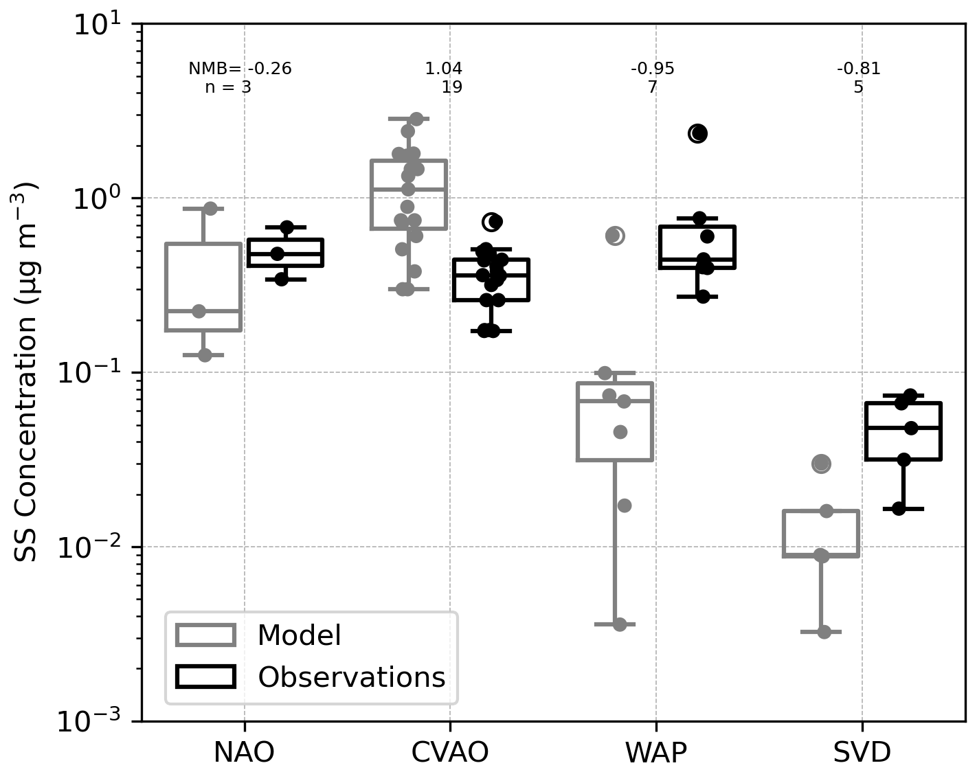
Figure 7 Box plot of observed versus ECHAM6.3–HAM2.3-simulated sub-micron sea salt concentration for the stations in Fig. 2 (see also Tables 2 and 4 for the location abbreviations and Table 5 for detailed information regarding the measurement data). Normalized mean bias (NMB) and sample size of observations are given for each station.

For comparison with measurements of marine organic aerosols, we account on the sub-micron aerosol concentration and estimated OMF from observations. For evaluating the model aerosol quantities PCHO_aer, DCAA_aer, and PL_aer, measured CCHO_aer, CAA_aer, and PG_aer were selected accordingly. In addition, measured organic mass (OM) concentrations are compared with the modelled total PMOA. Simulated and observed quantities for various stations were compiled into a multi-panel box plot in Fig. 8. A detailed description of the observational data and the discussion of our model results for each group is provided further below.

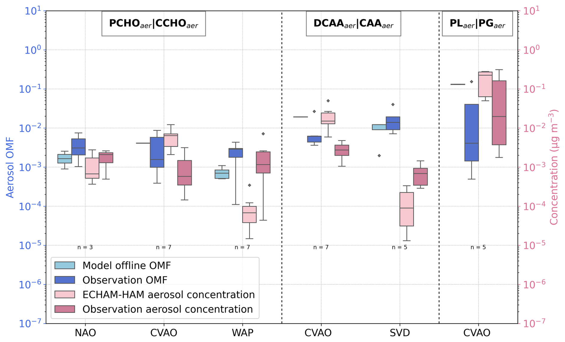
Figure 8 Box plot of the species-resolved, offline-computed OMF and ECHAM6.3–HAM2.3-simulated concentrations in contrast to the measured values. Sub-micron aerosols PCHO_aer, DCAA_aer, and PL_aer are compared to CCHO_aer, CAA_aer, and PG_aer, respectively, for the stations in Fig. 2 (see also Tables 2 and 4 for the compounds and location abbreviations, and Table 5 for detailed information regarding the measurement data). Dashed lines separate each group, and the name tags indicate the modelled marine aerosols separated by a straight bar from the measured aerosol components selected for the evaluation. Coral and light pink colours mark modelled values, whereas blue and dark pink indicate observations of OMF and aerosol concentration (in µg m⁻³), respectively. The sample size of observations (n) is included for all sites.

6.2.1 Sea salt

Owing to the linear relation between marine organic and sea salt aerosol emission mass flux (Eq. 10), the sea salt representation is essential to better understand the origin of model deviations in the analysis of the organic groups. Figure 7 illustrates the interpolated sub-micron SS concentration (gray boxes) in contrast to observations (black boxes). Observed quantities range between 0.06 and 1 µg m⁻³. Modelled results, extend beyond this range, spanning 10⁻³ to 2 µg m⁻³. Simulated values tend to underestimate the SS concentration for both northern and southern stations, whereas for the tropical location in Cape Verde (CVAO), simulations are larger than the observed amounts. The strongest negative normalized mean bias (NMB) occurs for the Western Antarctica Peninsula (WAP) followed by Svalbard (SVD) station with an underestimation of the median SS concentration of about 1 order of magnitude.

For the North Atlantic Ocean (NAO), observed sea salt (SS) concentrations lie within the modelled range and exhibit the lowest NMB. Because SS emissions depend on open-ocean conditions, for the polar stations (WAP, SVD, and NAO to some extent), the representation of sea ice cover, which is challenging in climate models, will strongly affect the SS emission compared to other ice-free oceanic regions. Additionally, the underestimation at WAP is supported by similar findings in the Southern Ocean by Regayre et al. (2020), who showed that only by tripling the simulated SS concentrations, obtained with the Gong (2003) source function, could the model align with observations. On the other hand, at CVAO, observed SS concentrations fall below the model’s first quartile. The elevated sea salt concentrations are likely driven by an excessively high mass emission flux, and ultimately, they may also be associated with inefficient wet deposition, a factor that could be especially significant in tropical regions.

A limitation that applies to the evaluation analysis of all aerosol species is that, as in other global aerosol–climate models, the turbulent transport and boundary layer height are parameterized. Therefore, variable wind conditions over height and time that influence the aerosol detection (measurement heights of less than 60 m) cannot be explicitly resolved by our model.

Large uncertainties persist in modelling sea spray aerosols within climate models (Grythe et al., 2014; Lapere et al., 2023), and regional models have shown varying performance of sea salt source functions among different stations (Barthel et al., 2019). Nevertheless, for the group of stations considered in this study, as well as for other locations worldwide (Tegen et al., 2019), the standard SS emission configuration in ECHAM6.3–HAM2.3 provides the most reasonable representation among the available schemes. Although the resulting biases in SS concentrations affect the predicted PMOA values, the evaluation of marine organics discussed in the following sections remains meaningful and valid despite the discrepancies in SS observations.

6.2.2 Carbohydrates

The organic mass fraction of PCHO_aer in nascent aerosols obtained from the offline calculation (coral boxes in Fig. 8) is comparatively higher at the tropical station (CVAO) with respect to NAO and WAP. In contrast, measured combined carbohydrates (CCHO_aer) (blue boxes in Fig. 8) are within the same range for all stations. For CVAO, the OMF median value is greater than the observed CCHO_aer. Conversely, an underestimation is seen for NAO. The discrepancies are significant for WAP with a negative mean model bias of −0.002, whereas for NAO and CVAO, OMF is within the same order of magnitude of observations.

Similarly, the simulated concentrations (light pink in Fig. 8) are lower than the observations (dark pink boxes in Fig. 8) for high-latitude sites. As a result, the aerosol concentrations are also underestimated for NAO and WAP, while higher values than the observations were modelled for CVAO. It is likely that the slight overestimation for CVAO is due to the relatively higher concentration of this biomolecule in seawater. Interestingly, there is no similar response for NAO or WAP for which the ocean biomolecules were over-represented by the model or in good agreement with the water samples. Possible causes for this contradicting pattern can be explained as follows.

Firstly, for NAO and WAP, aerosols were sampled while the ship was in motion. Therefore, aerosol samples were influenced by a much higher number of ocean areas than could be covered by surface seawater sampling. Secondly, relevant processes that favour the transfer of carbohydrates to the air are not included in the OCEANFILMS version used in this study. The under-representation of the organic fraction and concentration of carbohydrates in marine aerosols by the model seems to be a limitation of the monolayer Langmuir model, which neglects molecule interactions (Burrows et al., 2014). In addition to the aerosol measurements included in the present work, other studies employing different detection techniques have quantified even higher organic enrichment in aerosols attributed to carbohydrates (Russell et al., 2010; Frossard et al., 2014). Co-adsorption mechanisms facilitate the transfer to the aerosol phase of less surface-active compounds, such as polysaccharides or proteins, which are less enriched at the sea surface microlayer (SML). This occurs when such groups attach to the surfactants already coating the air bubble due to ionic interactions (Burrows et al., 2016; Hasenecz et al., 2019; Link et al., 2019).

Furthermore, given our model assumption, PCHO_aer is a fraction of CCHO_aer. Therefore, modelled dissolved acidic polysaccharides may not represent the total measured combined carbohydrates group but rather a fraction. Ultimately, given that aerosols are not collected under controlled conditions, concentrations may be affected by newly released polysaccharides by bacteria in the atmosphere (Zeppenfeld et al., 2021, 2023). Hence, CCHO_aer concentrations may also originate from secondary sources other than the primary oceanic sea spray emissions.

In addition to the aforementioned factors, the negative normalized mean biases found in the organic aerosol concentration for WAP (−0.95) and NAO (−0.26) can be associated with an underestimation of the simulated sea salt concentrations (Fig. 7). Sensitivity experiments with the ECHAM6.3–HAM2.3 model performed by Huang et al. (2018) demonstrated that when PMOA is emitted together with sea salt as sea spray, PMOA emissions are particularly sensitive to the sea salt source function selected.

6.2.3 Amino acids

The organic mass fractions of combined amino acids (CAA_aer) from measurements (Fig. 8 second panel) remain higher than that for CCHO_aer, a pattern that is also reflected in the offline calculated OMF. In contrast to observations, the median value of simulated OMF of DCAA_aer is slightly smaller for Svalbard (SVD) in comparison to CVAO. These OMF values tend to overestimate observations significantly for the tropical station, with a normalized mean bias of 1.19. However, for the northern site, model results are at the lower end of observations with small differences (NMB $=-\mathrm{0.46}$).

On the other hand, despite the OMF data from measurements in SVD remaining larger than that in CVAO, the opposite occurs for the aerosol concentration. The dissimilarities are explained by the higher mean sodium concentration in CVAO (Fig. 7), which compensates for the high occurrence of CAA_aer. The model nicely captures such regional characteristics for these stations. The concentration simulated at CVAO has a positive bias of 0.02 µg m⁻³ that is amplified as sea salt is overestimated in our model for this site (Fig. 7 with a bias of 0.7 µg m⁻³ for the SS sampled during the CAA_aer observations).

For the measurement campaign on Svalbard, the model bias is negative ($-\mathrm{6}\times {\mathrm{10}}^{-\mathrm{4}}$ µg m⁻³) and the median concentration is about 10-fold smaller than the observations. This may be related to the low sea salt content (SVD in Fig. 7), which we consider a determinant for the low DCAA_aer aerosol concentrations in the model.

6.2.4 Polar lipids

The scarce measurements of lipid aerosol within the simulated period limit our comparison to only the location of CVAO (Fig. 8 third panel). For this site, the measured concentrations and OMF exhibit significant disparities for PG_aer when compared to PCHO_aer and DCAA_aer. However, the model is capable of accurately representing the higher concentration of lipids in aerosols. Simulated OMF of PL_aer accounts for up to 84 % of total OMF for CVAO, whereas that of DCAA_aer and PCHO_aer is less than the 13 % and 3 %, respectively. As for van Pinxteren et al. (2023), we found that the lipids group has the highest contributions to the total marine organic aerosols.

Observations of PG_aer are widely spread, with a large interquartile range. The OMF values from measurements range between $\mathrm{4.9}\times {\mathrm{10}}^{-\mathrm{4}}$ and $\mathrm{1.5}\times {\mathrm{10}}^{-\mathrm{1}}$, whereas the aerosol concentration goes from $\mathrm{1.8}\times {\mathrm{10}}^{-\mathrm{3}}$ to $\mathrm{3.1}\times {\mathrm{10}}^{-\mathrm{1}}$ µg m⁻³. In contrast, simulated values do not present such variability. Modelled OMF lays at the upper end of values calculated from measurements ($\mathrm{1.3}\times {\mathrm{10}}^{-\mathrm{1}}$) with a mean bias of 0.09. Similarly, the aerosol concentration is also overestimated (MB =0.08 µg m⁻³).

The PL_aer group may encompass other subgroups rather than PG_aer. This could partially explain the overestimation of aerosol quantities by a factor of 3. However, these discrepancies, as previously mentioned, are strongly influenced by the misrepresentation of sea salt at this tropical station. Furthermore, in addition to the sea–air transfer via bubble bursting, there are other processes that influence the lipid concentration in aerosols. For instance, the presence of bacteria in marine aerosol particles could lead to atmospheric lipid production and degradation (Triesch et al., 2021b).

6.2.5 Total organic matter

Finally, to understand the contribution of marine aerosols (PMOA) to total organic matter given the background OC concentration, we examine the modelled organic concentration against observed OM_aer in sub-micron aerosol (Fig. 9). As previously introduced, OC originates from anthropogenic sources or biomass burning in the model. In contrast, simulated PMOA is the unique marine source to the aerosol organic matter.

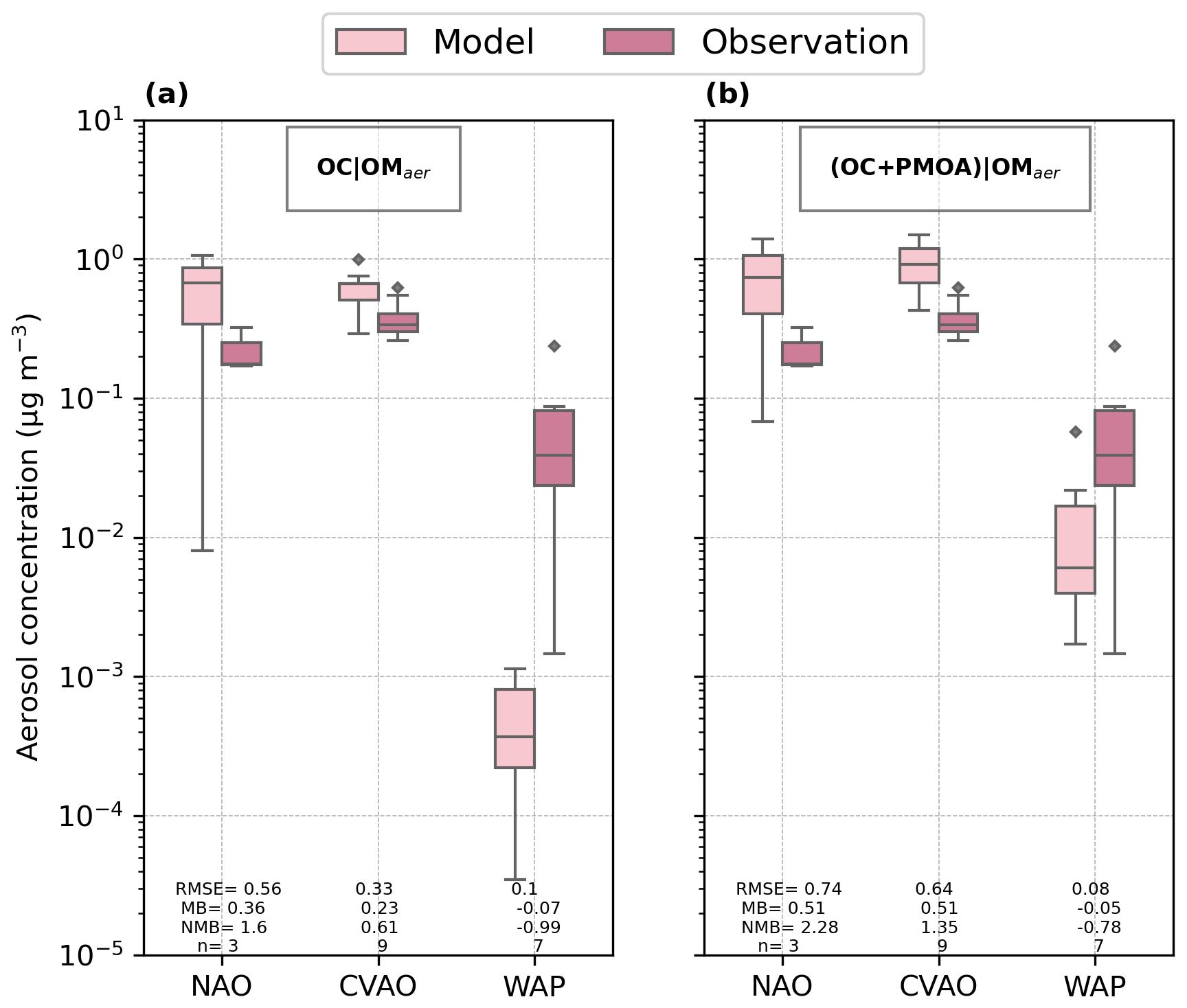
Figure 9 Box plot of the ECHAM6.3–HAM2.3-simulated sub-micron aerosol OC and (PMOA+OC) in contrast to measured OM_aer for the stations in Fig. 2 (see also Tables 2 and 4 for the compounds and location abbreviations, and Table 5 for detailed information regarding the measurement data). The modelled aerosol quantity is separated by a straight bar from the measured aerosol components selected for the evaluation. Root mean square error (RMSE) and the mean bias (MB) (in units of µg m⁻³), the normalized mean bias (NMB), and sample size (n) are given for each station (see Table A1 for formulas to calculate the statistical indexes).

The observed aerosol concentrations are highest for CVAO and NAO (dark pink boxes in Fig. 9). For the Antarctica station (WAP), quantities are approximately 1 order of magnitude smaller compared to the other sites. Simulated OC (Fig. 9a) tends to slightly overestimate the observed organic matter concentration for NAO and CVAO, being more pronounced for the northernmost location. At the tropical site, modelled values are within the same range as observations, whereas for NAO, values concentrate at the upper end of measured quantities. Lastly, WAP is the only area in which organic matter is poorly represented when the local marine aerosols are not considered.

Note that the assumptions introduced here to calculate the OM_aer are based on measured OC, which can be variable, and are thus a source of error. What is more important here, however, is the fact that the sites in the northern and subtropical Atlantic are strongly affected by anthropogenic and biomass burning sources, which actually dominate and can lead to high levels of organic carbon. In accordance with the results of the detailed evaluation by Tegen et al. (2019), the non-marine contributions in both regions can vary considerably in ECHAM6.3–HAM2.3. Based on this, we consider the overestimations of OC at NAO and CVAO to be likely related to uncertainties in biomass burning aerosol emissions, whose representation remains challenging for aerosol–climate models.

As a result of accounting for PMOA as an additional source of organic aerosols (Fig. 9b) the total simulated concentration increases at NAO and CVAO leading to a rise in model biases and errors. Conversely, a notable improvement is observed in the more pristine region in the Southern Ocean (WAP) where the absolute mean bias and normalized mean bias decreased by approximately 21 % to 29 % when considering PMOA. Overall, across the three stations, the correlation between modelled and observed organic matter remains moderate, with little change upon incorporating PMOA (decreasing slightly from 0.61 for OC to 0.57 for OC + PMOA). Nevertheless, this analysis highlights the quantifiable relevance of PMOA and its significant contribution to organic aerosol mass in remote oceanic regions.

Despite the overall uncertainties and model biases in representing the organic fraction and aerosol concentrations for point locations, the modelled values range in the same order of magnitude as the observations for most stations. Furthermore, our model can still capture the differential aerosol enrichment of the biomolecule groups also visible in measurements, in which PL_aer predominates in the aerosols with contributions of up to 2 orders of magnitude greater than PCHO_aer and DCAA_aer.

6.3 Comparison of PMOA with in situ aircraft measurements

In order to show the capability of the model to represent PMOA in remote oceanic regions, where ground-based measurements are barely feasible or species-resolved quantities are unavailable, we compare the simulated PMOA concentrations with organic aerosol mass from ATom aircraft observations. The comparison in Fig. 10 clearly shows how the model performance improves when PMOA is considered in contrast to the configuration without. For the SPMOAoff case, the concentration of the OC tracer is compared, while for the SPMOAon simulation it is the total OC and PMOA. Note that modelled OC only comprises emissions from anthropogenic sources and biomass burning.

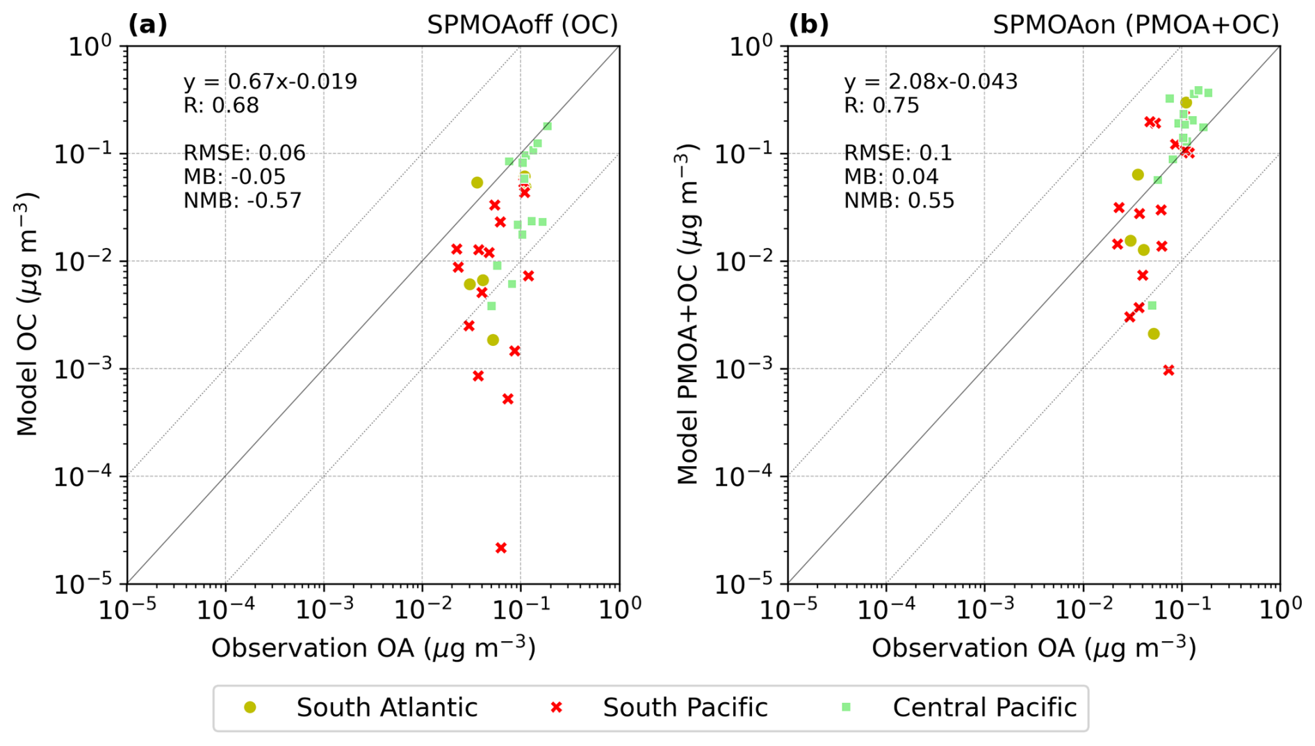
Figure 10 Scatter plot of the comparison of aerosol concentration daily averages of ECHAM6.3–HAM2.3-simulated PMOA and organic aerosol aircraft observations (ATom data) for the (a) SPMOAoff and (b) SPMOAon experiments. The data were grouped per region as in Fig. 3. Observed and measured quantities represent the concentration at standard temperature and pressure conditions (273 K, 1 atm). Root mean square error (RMSE) and the mean bias (MB) (in units of µg m⁻³), the normalized mean bias (NMB), the correlation coefficient (R), and sample size are given for each station. The formulas to calculate the statistical indexes may be found in Table A1.

Overall, the correlation with observations is high for both experiments. However, a notable underestimation is observed for the SPMOAoff case, specially for the South Pacific. Model values increase toward a better agreement when PMOA is added and the correlation coefficient rises from 0.67 to 0.74 with a significant improvement for several sites. The independent model biases per region indicate that the model biases are considerably reduced for the South Pacific and Atlantic oceans. Interestingly, adding PMOA leads to an overestimation of the modelled organic aerosols in the central Pacific. This is surprising, since the aerosol load in this region is expected to be governed by local sources. Possibly, the uncertainties in OC emission sources could explain this, as long-range-transported aerosols from the Asian and Australian continents might be the origin of the initially elevated OC aerosol concentrations in this region.

These results are in accordance with a previous study by Pai et al. (2020), who found a strong influence of primary marine organic aerosols of the remote marine boundary layer. Their model simulations, however, tend to overestimate the observed values, with larger biases than in this study. This might be the result of the differences in the marine aerosol emission parameterization (using Gantt et al., 2015), and further atmospheric transformation processes are taken into account.

Note that measured organic aerosols (OAs) from ATom aircraft data encompass multiple aerosol sources and types. The OA includes primary and secondary organic aerosol particles (Hodzic et al., 2020) which could not be disentangled from the original dataset. In our model simulations, only primary aerosols are considered, so the secondary aerosol formation resulting from chemical transformation of the respective precursor species is missing in the comparison on the modelling side. Nonetheless, our findings suggest that by adding PMOA to primary non-marine OC, the model estimates are already significantly improved for southern oceanic regions.

Lastly, the model coarse temporal and spatial resolution is a major source of uncertainties for this comparison. The large daily standard deviation in measured OA indicates the strong variability in the data, which, given our model limitation, cannot be captured. Nonetheless, our results show that by including PMOA, our model represents better the organic aerosol in the lower atmosphere of remote southern oceanic regions. Moreover, seasonal variability, which was not considered here, seems to be a critical factor when validating aerosol model results with ATom data (Gao et al., 2022).

7 Summary and conclusions

In this study, primary marine organic aerosols are included in the global aerosol–climate model ECHAM6.3–HAM2.3 to investigate their emission characteristics and distribution. The representation of organic mass fraction is based on the marine emission scheme OCEANFILMS by Burrows et al. (2014). We account for the contribution of three main marine biomolecule groups in the ocean relevant for the aerosol phase (dissolved acidic polysaccharides (PCHO_sw), dissolved combined amino acids (DCAA_sw), and polar lipids (PL_sw)). Marine quantities are based on phytoplankton-exuded carbon calculated by the ocean biogeochemistry model FESOM2.1–REcoM3 and serve as bottom boundary condition to the atmospheric model.

The simulated PCHO_sw is the most abundant group in seawater, followed by DCAA_sw and PL_sw, both of which exhibit lower contributions to the extracellular dissolved organic carbon. The abundance and amounts of molecules are well represented in the simulations compared to worldwide in situ seawater measurements.

The individual marine groups show a diverse global distribution. PL_sw ocean concentrations are generally higher in biologically active regions, whereas PCHO_sw and DCAA_sw groups predominate in subtropical and tropical waters. The distribution of the organic mass fraction of aerosols closely resembles that of the concentrations of biomolecules in oceans. Nevertheless, a differential enrichment in the aerosols was detected. Given the high air–water surface affinity of lipids, this group dominates the organic mass in aerosols, while PCHO_aer and DCAA_aer tend to be significantly lower in magnitude.

The seasonal patterns of the marine biomolecule and organic aerosol mass fraction were additionally examined. For polar regions, seasonality is remarkable in contrast to mid- and equatorial latitudes. The greatest contribution of the three organic groups occurs during summer in each hemisphere, and the values remain invariant for the Equator. In a follow-up study, we will comprehensively examine the distinctive characteristics of the Arctic and the evolution of marine biomolecules and PMOA over the past decades, owing to the distinct significance of this region and its prominent alterations in response to changing climate conditions.

The global aerosol model simulations indicate that PMOA emission fluxes are sensitive to multiple factors. Among them, the marine biological activity and surface wind conditions are mainly controlling the occurrence of PMOA. Due to elevated wind speeds, the emission fluxes in the North Atlantic, North Pacific, and Indian waters tend to be stronger. The model estimate of the aggregated PMOA emission globally is 12.1 Tg yr⁻¹, corresponding to an atmospheric burden of 0.075 Tg.

Furthermore, the modelled mass concentrations of the primary marine organic aerosol were thoroughly evaluated using observations. A comparative analysis of PMOA against organic aerosols from NASA's ATom aircraft campaigns indicated that the model has better correlation for remote Southern Hemisphere oceans when PMOA is included. The species-resolved aerosol evaluation showed that the model could capture the differential organic enrichment in aerosols. Nevertheless, further improvements are needed for the aerosol–climate model. For instance, the underestimation of sea salt emissions affected a more correct representation of the PMOA concentrations. Here, more detailed emission functions of sea salt or sensitivity studies with multiple source functions could lead to better estimates in the future (e.g. Grythe et al., 2014; Albert et al., 2016). Although the uncertainties are large across models and source functions, some improvements in certain regions may be achieved. Moreover, adjusting OCEANFILMS parameters to better characterize the physicochemical properties of the biomolecules studied here could lead to a more accurate representation of the organic fraction in aerosols.

The different emission and transport patterns found in this modelling study suggest that the distinct components of PMOA may exert a differentiated influence on cloud and precipitation formation. Our research provides a model setup that considers diverse marine organic aerosol groups. This model setup will be further developed to incorporate the significance of individual groups or aggregated PMOA in aerosol–cloud interaction processes in future studies. The capability of regional grid refinements for the biogeochemical model provides a vast scope for the approach presented here to compute biomolecules as boundary conditions for a high-resolution aerosol–cloud model simulation. This could be particularly interesting for Arctic studies, as it enables the incorporation of spatial fine structures, such as phytoplankton blooms along marginal ice zones, and evaluate the effect of mixed-phase clouds in the Arctic climate.

Appendix A: Statistical index formulas

Table A1 Formulas of statistic indexes. M_i and O_i refer to the model results and observational data i for each station or region. N is the data sample size.

Appendix B: Maps of monthly biomolecule quantities

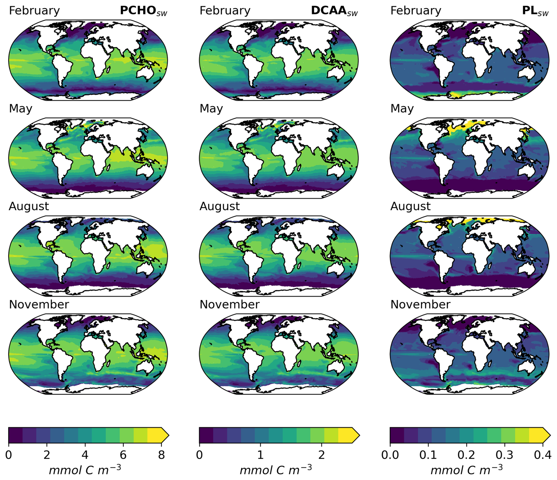
Figure B1 Maps of monthly-averaged ocean carbon concentration of PCHO_sw (first column), DCAA_sw (second column), and PL_sw (third column) for February, May, August, and November as a multiannual mean for the period 1990–2019 for sea-ice-free conditions (SIC < 10 %).

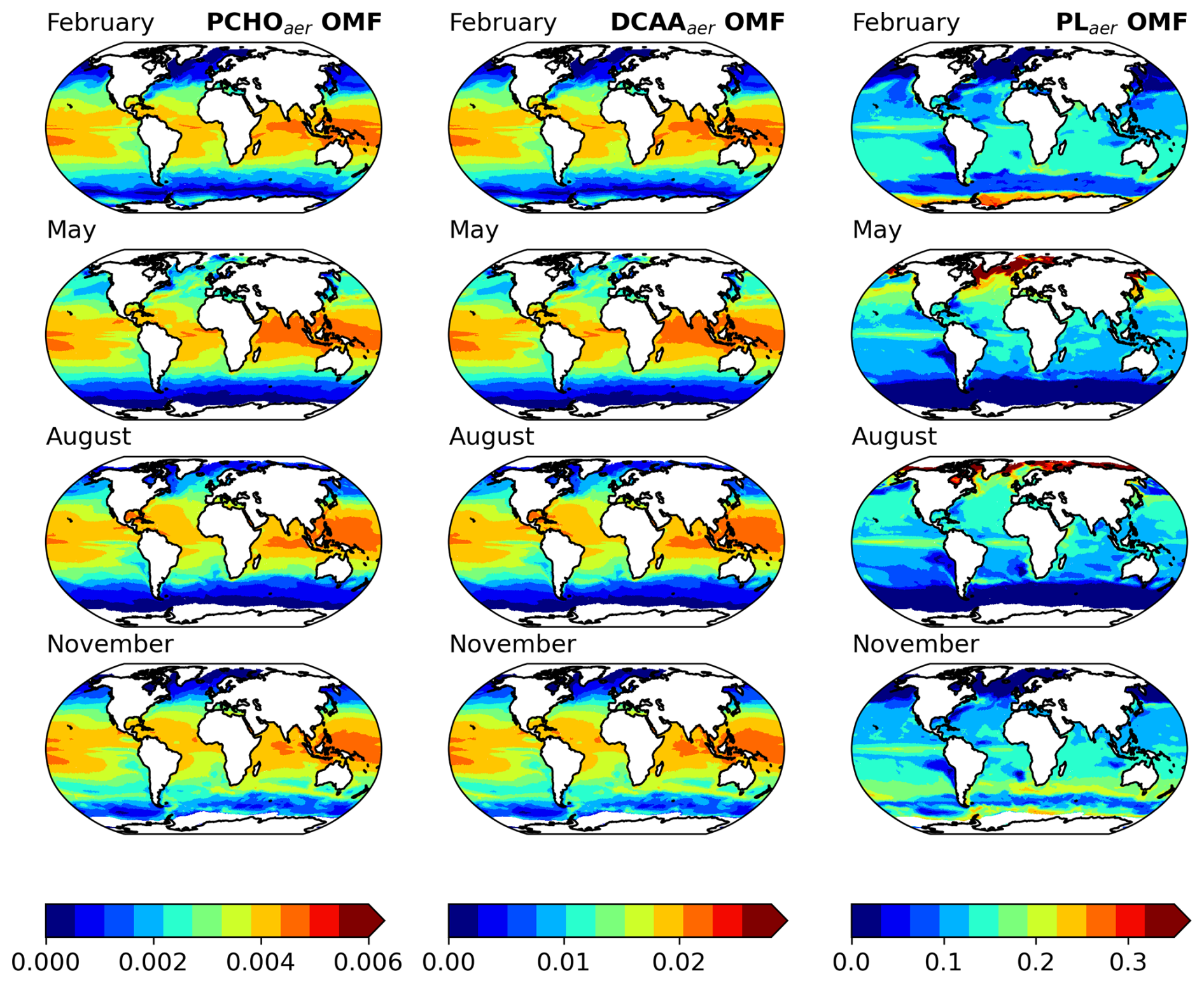
Figure B2 Maps of monthly-averaged, offline-computed OMF of PCHO_aer (first column), DCAA_aer (second column), and PL_aer (third column) for February, May, August, and November as a multiannual mean for the period 1990–2019 for sea-ice-free conditions (SIC < 10 %).