Estimation of above- and below-ground ecosystem parameters for DVM-DOS-TEM v0.7.0 using MADS v1.7.3

The permafrost region contains a significant portion of the world's soil organic carbon, and its thawing, driven by accelerated Arctic warming, could lead to substantial release of greenhouse gases, potentially disrupting the global climate system. Accurate predictions of carbon cycling in permafrost ecosystems hinge on the robust calibration of model parameters. However, manually calibrating numerous parameters in complex process-based models is labor-intensive and is complicated further by equifinality – the presence of multiple parameter sets that can equally fit the observed data. Incorrect calibration can lead to unrealistic ecological predictions. In this study, we employed the Model Analysis and Decision Support (MADS) software package to automate and enhance the accuracy of parameter calibration for carbon dynamics within the coupled Dynamic Vegetation Model, Dynamic Organic Soil Model, and Terrestrial Ecosystem Model (DVM-DOS-TEM), a process-based ecosystem model designed for high-latitude regions. The calibration process involved adjusting rate-limiting parameters to accurately replicate observed carbon and nitrogen fluxes and stocks in both soil and vegetation. Gross primary productivity, net primary productivity, vegetation carbon, vegetation nitrogen, and soil carbon and nitrogen pools served as synthetic observations for a black spruce boreal forest ecosystem. To validate the efficiency of this new calibration method, we utilized model-generated synthetic and actual observations. When matching model outputs to observed data, we encountered difficulties in maintaining mineral soil carbon stocks. Additionally, due to strong interdependencies between parameters and target values, the model consistently overestimated carbon and nitrogen allocation to the stems of evergreen trees. This study demonstrates the calibration workflow, offers an in-depth analysis of the relationships between parameters and observations (synthetic and actual), and evaluates the accuracy of the calibrated parameter values.

1 Introduction

The permafrost region contains 1440–1600 pg of organic carbon in its soils, representing nearly half of the world's soil organic carbon pool (Hugelius et al., 2014; Schuur et al., 2022). Accelerated warming in the Arctic leads to permafrost thaw, resulting in the decomposition and potential release of a substantial portion of this stored carbon as greenhouse gases, significantly impacting the global climate system (Natali et al., 2021; Schuur et al., 2022; Treharne et al., 2022). The permafrost carbon–climate feedback remains one of the largest sources of model uncertainty for future climate predictions, as critical ecological and biogeochemical processes are poorly represented and constrained in ecosystem models, if included at all (McGuire et al., 2016, 2018; Schädel et al., 2024). A significant portion of this uncertainty stems from parameter uncertainty, particularly in rate-limiting factors that control biogeochemical cycles, which are challenging to measure directly and can vary considerably across spatial and temporal scales (Koven et al., 2015; Mishra et al., 2021). These uncertainties propagate through model simulations, contributing to a wide range of projected permafrost carbon emissions (Lawrence et al., 2015; McGuire et al., 2018).

When compared to structural uncertainty (which arises from incomplete or simplified representations of ecological processes) and input data uncertainty (resulting from limited or biased forcing datasets), parameter uncertainty is particularly pervasive and difficult to constrain (Euskirchen et al., 2022; Fisher and Koven, 2020; Luo et al., 2016). While structural uncertainties limit a model's ability to fully capture real-world processes, parameter uncertainties directly alter numerical outputs, often amplifying variations in projections (Fisher and Koven, 2020; Turetsky et al., 2020). Models are particularly sensitive to parameter uncertainties given the complexity and variability of the processes they simulate, including soil thermal dynamics, vegetation feedbacks, and hydrological interactions (Andresen et al., 2020; Harp et al., 2016; Koven et al., 2015). While structural improvements to model frameworks are ongoing, addressing parameter uncertainty through robust calibration methods remains an essential and complementary step in enhancing the accuracy and reliability of model outputs (Fisher and Koven, 2020; Luo et al., 2016). Addressing these uncertainties through the development of effective calibration techniques is essential for refining predictions of permafrost dynamics and better constraining future permafrost carbon–climate feedbacks (McGuire et al., 2018; Mishra et al., 2021).

Calibration involves estimating and adjusting model parameters to enhance the agreement between model outputs and observed data, with the model serving as a mathematical representation of ecological and physical processes (Rykiel, 1996). These parameters are often rate or transport constants that are onerous or impractical to estimate empirically, though model outputs can be highly sensitive to them. Since many model representations are grounded in physics, generalized physical laws are often used to describe ecological and cryo-hydrological processes. Typically, model outputs are validated against data from laboratory experiments, idealized mathematical models, or site-specific observations, also referred to as target data. During this validation, model parameters are adjusted so that model outputs match the target data. The validated model is then applied to broader geographic locations and/or different time periods, assuming that the validation data represent the environment or ecosystem for which the parameters were calibrated.

Parameter calibration for complex process-based models is often constrained by the significant labor required and the limited availability of sites with the necessary observations, especially in permafrost regions (Birch et al., 2021; Virkkala et al., 2019). Despite these challenges, process-based models remain essential because they encapsulate our current understanding of ecosystem functions and structures, serving as powerful tools for extrapolation. The assumption of representativeness is intrinsic to these models, as they are designed to simulate processes that reflect our best understanding of ecosystem dynamics, allowing for their application beyond the individual sites where they were initially parameterized. The approach of extrapolating model parameterization for ecosystems of the same type across wider regions is standard and widely used within ecosystem modeling communities (Matthes et al., 2025; McGuire et al., 2018). Additionally, the role of ecosystem diversity in the spatiotemporal patterns of ecosystem carbon dynamics in the permafrost region has been characterized by numerous empirical studies (Euskirchen et al., 2014; Melvin et al., 2015) and evaluated by modeling investigations (Lara et al., 2016). Therefore, a critical step in improving model accuracy involves calibrating the model against a suite of data for a representative diversity of ecosystem types in the Arctic where observations are available. To prepare an ecosystem model for this extensive calibration task, it is essential to develop robust calibration tools and methods that can automate the process of efficiently optimizing model parameters.

Another well-known and significant issue in optimizing model parameters through calibration, also referred to as parameter estimation or optimization, is the existence of equifinality (Jafarov et al., 2020; Nicolsky et al., 2007; Tran et al., 2017). Parameterization equifinality occurs when different sets of parameter values result in the same or similar model predictions, given that the model, forcing data, and observations used in calibration are the same (Beven and Freer, 2001). Model equifinality can subsequently lead to different outcomes in model projections. With the aim of addressing the issue of equifinality, we run the model using randomly varied parameter values within the given range. If the majority of calibration tests with different initial guesses yield a good fit with observations and result in optimal parameter sets that are similar or closely aligned, this increases confidence that the recovered parameter set is indeed optimal. This approach mitigates the risk of converging on a local minimum and ensures a more robust and reliable parameter estimation process (Hansen, 1998).

Various methods have been employed to improve the calibration of model parameters across multiple scientific disciplines, utilizing sophisticated techniques and integrating diverse data sources such as remote sensing and field measurements while accounting for model and data uncertainty (Dietze et al., 2018; Efstratiadis and Koutsoyiannis, 2010; Luo et al., 2016). Optimization-based inverse methods have been used successfully to calibrate parameters in physical models, including snow properties and subsurface thermo-hydrological properties (Jafarov et al., 2014, 2020) as well as soil properties for permafrost modeling (Nicolsky et al., 2007, 2009). However, inverse modeling can become computationally intractable when applied to complex process-based models (Linde et al., 2015).

Markov chain Monte Carlo (MCMC) and data assimilation (DA) techniques have been employed to optimize model parameters by synchronizing model outputs with observed data, thereby enhancing model prediction accuracy (Brunetti et al., 2023; Fer et al., 2018; Xu et al., 2017). These methods often leverage Bayesian inference to address structural uncertainties within models. Nonetheless, the computational demand required to conduct MCMC simulations can outweigh the gains in model accuracy, particularly when dealing with complex process-based models with slow turnover rates that necessitate long simulations to reach equilibrium.

In recent years, DA techniques have been applied to optimize both model state variables (Fox et al., 2018; Ling et al., 2019) and parameters (Bloom et al., 2016; Peylin et al., 2016; Scholze et al., 2016; Schürmann et al., 2016). However, DA also encounters challenges related to unbalanced outputs and the need for extended simulations to achieve equilibrium. Persistent issues include the incorrect characterization of the error covariance matrix, which can lead to inaccurate posterior parameter values due to unaccounted-for model structural errors and observation biases (MacBean et al., 2016; Wutzler and Carvalhais, 2014).

Various surrogate-based optimization approaches have been proposed to alleviate the computational burden associated with parameter calibration (Koziel et al., 2011; Queipo et al., 2005). Surrogate models, also known as reduced-order models, simplify certain physical processes to approximate the underlying dynamics of the real model while being computationally less demanding (Forrester et al., 2006). By simplifying specific aspects of the model, surrogate models retain essential characteristics of the original system, allowing for faster and more efficient calibration without significantly compromising accuracy (Razavi et al., 2012; Regis and Shoemaker, 2007). However, simplifying complex models presents significant challenges. It is often unclear which assumptions can be made safely and which should be avoided, potentially leading to a loss of model accuracy. Surrogate models must carefully balance the tradeoff between simplification and the retention of critical model characteristics to ensure reliable performance. This complexity necessitates rigorous validation to confirm that the surrogate model provides an adequate approximation of the real system without introducing significant errors.

In recent years, machine-learning-based emulators, often referred to as “models of models”, have emerged as a promising approach to reduce the computational burden associated with parameter calibration in complex ecosystem models (Castelletti et al., 2012; Fer et al., 2018; Reichstein et al., 2019). These emulators aim to approximate the outputs of physical and process-based models by learning the relationships between model inputs and outputs through multidimensional matrices, significantly enhancing computational efficiency. Unlike traditional surrogate models, which simplify the physical processes within a model, emulators strive to mimic the full complexity of the original model while requiring less computational power. For instance, Dagon et al. (2020) utilized artificial neural networks to emulate the Community Land Model version 5 outputs, focusing on biophysical parameter estimation and global calibration. By integrating machine learning techniques, they were able to explore parameter spaces more efficiently and achieve better alignment with observed data. This method demonstrates the potential of machine learning emulators to improve the accuracy and efficiency of parameter calibration in ecosystem models, particularly when faced with the challenge of high computational demands.

To facilitate the automation of the calibration process while minimizing computational demands and avoiding the oversimplification of ecological processes and feedbacks, we employed a nonlinear least-squares approach for our calibration. We utilized the Model Analysis and Decision Support (MADS) software package (Barajas-Solano et al., 2015; O'Malley and Vesselinov, 2015) for parameter calibration of a terrestrial ecosystem's permafrost-enabled model. MADS has been actively developed since 2010, and its transition to the Julia programming language has provided automatic differentiation capabilities suitable for calibration problems, improving computational efficiency (Vesselinov, 2022).

In this study, we developed an automated parameter calibration method for a process-based terrestrial ecosystem model developed for high-latitude regions and characterized by a high level of complexity. To demonstrate its efficacy, we utilized synthetic data and evaluated the capacity of the calibration method to recover the data after perturbing initial guesses (a given set of parameters) using random sampling. The model was run using known parameter values, and the resulting outputs were treated as observations. The primary objective was to illustrate that the parameter calibration method could recover the synthetic parameter set successfully. The secondary objective was to optimize and reduce the labor and time associated with manual parameter calibration. We developed and tested our calibration method using the coupled Dynamic Vegetation Model, Dynamic Organic Soil Model, and Terrestrial Ecosystem Model (DVM-DOS-TEM) and tested our approach using synthetic and site observations at a black spruce forest site, which is a dominant community type in the interior of Alaska. The final objective was to evaluate the calibration method using the dataset presented in Melvin et al. (2015).

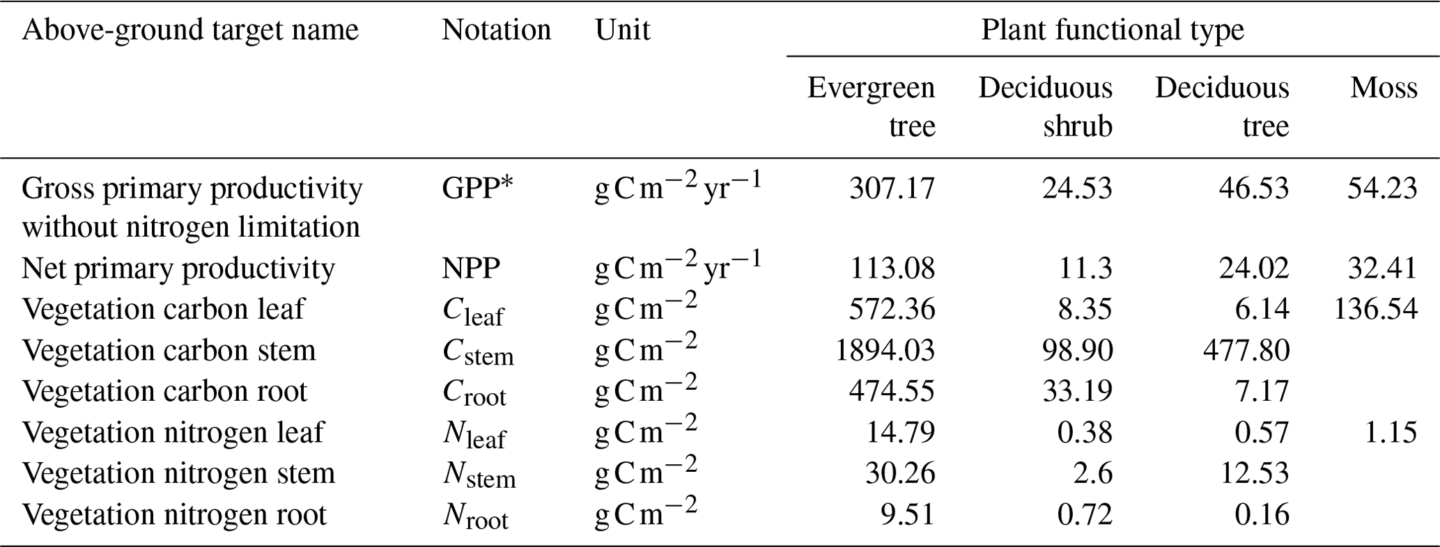
Table 1 Synthetic vegetation target values for the black spruce forest site used in the parameter calibration process.

2 Methods

2.1 Black spruce forest site

Approximately 39 % of the interior of Alaska is covered by evergreen forest stands dominated by white or black spruce, and 24 % is covered by deciduous forest stands dominated by Alaska paper birch or trembling aspen (Calef et al., 2005; Jean et al., 2020). In our study, we developed a model calibration for a black spruce (Picea mariana) forest community type, using observations collected at a site located within the Tanana Valley State Forest just outside Fairbanks, Alaska (64°53^′ N, 148°23^′ W). Carbon (C) and nitrogen (N) cycling and environmental monitoring in this forest stand were originally observed by Melvin et al. (2015). The stand resulted from a self-replacement succession trajectory following the 1958 Murphy Dome fire, which covered 8930 ha.

2.2 DVM-DOS-TEM description

The DVM-DOS-TEM is a process-based biosphere model designed to simulate biophysical and biogeochemical processes between the soil, vegetation, and atmosphere. The DVM-DOS-TEM has been applied extensively in Arctic and boreal ecosystems in permafrost and non-permafrost regions (Briones et al., 2024; Euskirchen et al., 2022; Genet et al., 2013, 2018; Jafarov et al., 2013; Yi et al., 2009, 2010). This model focuses on representing C and N cycles in high-latitude ecosystems and how they are affected at seasonal (i.e., monthly) to centennial scales by climate, disturbances (Genet et al., 2013, 2018; Kelly et al., 2013), biophysical processes such as soil thermal and hydrological dynamics (McGuire et al., 2018; Yi et al., 2009; Zhuang et al., 2002), snow cover (Euskirchen et al., 2006), and plant canopy development (Euskirchen et al., 2014). Modeled vegetation is structured into three tiers: (1) the community type (CMT) represents the land cover class and characterizes vegetation composition and soil structure at the grid-cell level (spatial unit, e.g., black spruce forest, tussock tundra, or bog), (2) plant functional types (groups of species sharing similar functional traits) characterize the vegetation composition of every CMT (e.g., a black spruce forest community would be composed of evergreen trees, deciduous shrubs, and sphagnum and feather moss plant functional types), and (3) plant structural compartments (leaves, stems, and roots). The soil column is split into multiple horizons (fibric, humic, mineral, and rock/parent material). Every horizon is split into multiple layers for which C, N, temperature, and water content are simulated individually. The biophysical processes represented in the DVM-DOS-TEM include radiation and water fluxes between the atmosphere, vegetation, snow cover, and soil column. Soil moisture and temperature are updated at a pseudo-daily time step (from linear interpolation of monthly climate forcings). A two-directional Stefan algorithm is used to predict the positions of freezing–thawing fronts in the soil. The Richards equation is used to calculate soil moisture changes in the unfrozen layers of soil. Both the thermal and hydraulic properties of soil layers are affected by their water content (Yi et al., 2009, 2010; Zhuang et al., 2002). The ecological processes represented in the DVM-DOS-TEM include C and N dynamics for every plant functional type (PFT) of the vegetation community and every layer of the soil column. C and N dynamics are driven by the climate, atmospheric CO₂ content, soil and canopy environment, and wildfire occurrence and severity. C and N cycles are coupled in the soil and the vegetation processes. The growth primary productivity (GPP) of each PFT is limited by the N availability. When resources in N are limited, GPP is downregulated for all PFTs based on a comparison of N demand (N required to build new tissues) and N supply in the ecosystem (Euskirchen et al., 2009). C and N from the litterfall are divided into above-ground and below-ground classes. Above-ground litterfall is only assigned to the top layer of the soil column, while below-ground litterfall (root mortality) is assigned to different layers of the three soil horizons based on the fractional distribution of fine roots with depth.

2.3 Synthetic data

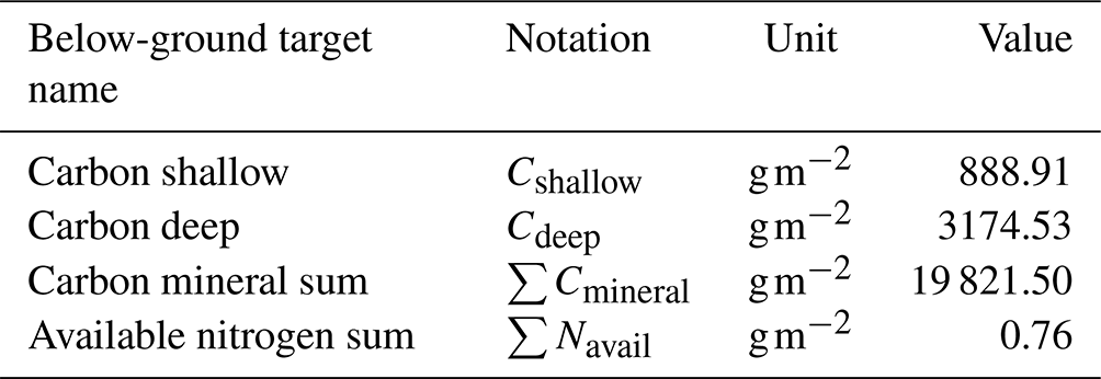
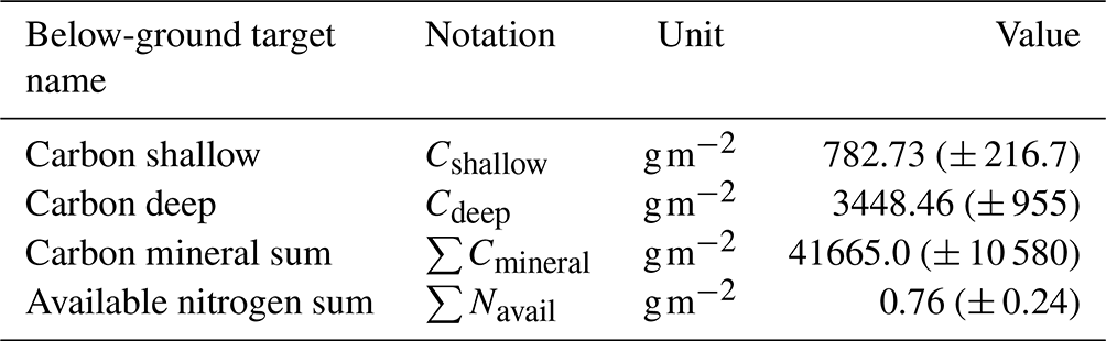
We used GPP without N limitation (GPP^∗), net primary productivity (NPP), vegetation C stocks, and vegetation N stocks by compartment (i.e., roots, stems, and leaves) as the synthetic observations shown in Table 1. Synthetic observations are model-generated data that simulate actual measurements using known parameter values, referred to as synthetic target values. To generate these target values, we used existing parameters and the setup described in Sect. 2.3. The target values shown in Table 1 represent the state of the ecosystem where vegetation and below-ground C stocks are in a steady state. Table 2 includes the below-ground target values. The model was previously calibrated manually using observations from the site. The actual observations were collected and prepared from the measured data at the site and from the existing literature and published datasets. Data preprocessing was required before the time series data could be analyzed. Preprocessing was performed to identify and resolve missing data, inconsistencies, and potential outliers. In addition, site observations were aggregated to a monthly resolution to match the temporal resolution of the model outputs, and unit transformations were applied when needed to standardize the units of each variable. Target values for the site were compiled from various data literature sources containing information on C and N stocks, plant biomass, soil horizon depths, and productivity. However, following the initial calibration, the model outputs were similar but did not exactly match the target observations. As stated above, we choose synthetic targets because we know a set of parameters used to produce them and can compare how closely we can recover known parameter values. Therefore, we used the actual model output as our synthetic target values.

Table 2 Synthetic below-ground target values for the black spruce forest site used in the parameter calibration process.

2.4 Input data used for equilibrium runs

The driving inputs for the DVM-DOS-TEM comprise spatial distributions of CMTs, landforms, and mineral soil texture. These initialization data were forced to field observations at the study site (Melvin et al., 2015). The spatiotemporal dynamics of the model are driven by an annual time series of atmospheric CO₂ concentration (not spatially explicit), an annual time series of spatially explicit distributions of fire scars and dates, and a spatially explicit monthly time series of climate, including mean air temperature, total precipitation, net incoming shortwave radiation, and vapor pressure (Genet et al., 2018). For the present study, we use historical climate data from 1901 to 2015, sourced from the Climatic Research Unit time series version 4.0 (CRU TS4.0; Harris et al., 2014) and downscaled at a 1 km resolution using the delta method (Pastick et al., 2017). For the equilibrium run, the model was driven using the averaged climate forcings from the 1901–1930 period for the study site location, repeated continuously for a sufficient period so that equilibrium of vegetation and below-ground C and N fluxes and stocks was achieved. The resulting modeled ecosystem state for each site is then used to initialize historical simulations. However, the calibration process described here only utilized outputs from the equilibrium.

2.5 MADS parameter calibration

We employed the MADS software package for parameter calibration of the DVM-DOS-TEM, aiming to minimize the discrepancy between synthetic target and modeled data at the selected site (Barajas-Solano et al., 2015; O'Malley and Vesselinov, 2015). Since its inception in 2010, MADS has undergone active development, including a transition to the Julia programming language, which supports automatic differentiation suitable for calibration problems (Vesselinov, 2022).

The MADS package utilizes the Levenberg–Marquardt (LM) algorithm (Levenberg, 1944; Marquardt, 1963; Pujol, 2007) to minimize the difference (the sum of squared residuals) between observations and modeled predictions. In Fig. S1 in the Supplement, we provide more details on the LM algorithm. The LM optimization method was designed to solve nonlinear least-squares optimization or minimization problems, which are common in the field of history matching, model inversion, curve fitting, and parameter estimation. It combines two approaches: the first-order steepest-descent gradient method and the second-order Gauss–Newton method. This steepest-descent gradient method updates parameter values in the direction opposite to the gradient, so it is generally efficient at finding local minima. The Gauss–Newton method assumes that, in a region close to the solution, the solved objective function behaves quadratically.

The algorithm begins by selecting an initial estimate for the parameters that need to be optimized (Fig. S1). This initial guess is important as it sets the starting point for the optimization process. In our experiment, the initial guess is randomly generated from within the provided range near “true” parameter values. Alternatively, users can provide the initial guess. However, exploring a set of random initial guesses provides an efficient approach to exploring the parameter space and discrimination between local and global minima. In the LM method, we set the damping parameter (the Marquardt lambda) to 0.01. This parameter helps to adjust the steps taken during the optimization process, maintaining a balance between the two optimization strategies (the first- and second-order techniques discussed above).

The main advantages of the LM method are its robustness and minimal computational demands. It effectively handles ill-conditioned problems where other optimization methods might fail (Lin et al., 2016; Pujol, 2007). Additionally, for problems well-suited to the Gauss–Newton method, the LM method often converges faster than the gradient descent, making it an efficient choice for many nonlinear least-squares problems.

Figure 1 Schematics of the DVM-DOS-TEM parameters and targets in the calibration process.

The disadvantage of the LM method is its sensitivity to the initial parameter guesses, potentially affecting its efficiency and convergence (Transtrum and Sethna, 2012). In these cases, MADS provides alternative efficient approaches to address these computational challenges, such as (1) initialization of the calibration with random initial guesses, (2) multiple restarts of the LM algorithms throughout the minimization process, and (3) exploration of a series of alternative values for various parameters controlling LM performance (Lin et al., 2016). In addition, the compute speed deteriorates with the higher number of parameters used in the calibration. It requires the computation of the Jacobian matrix and its pseudo-inverse, which can be computationally expensive for large-scale problems.

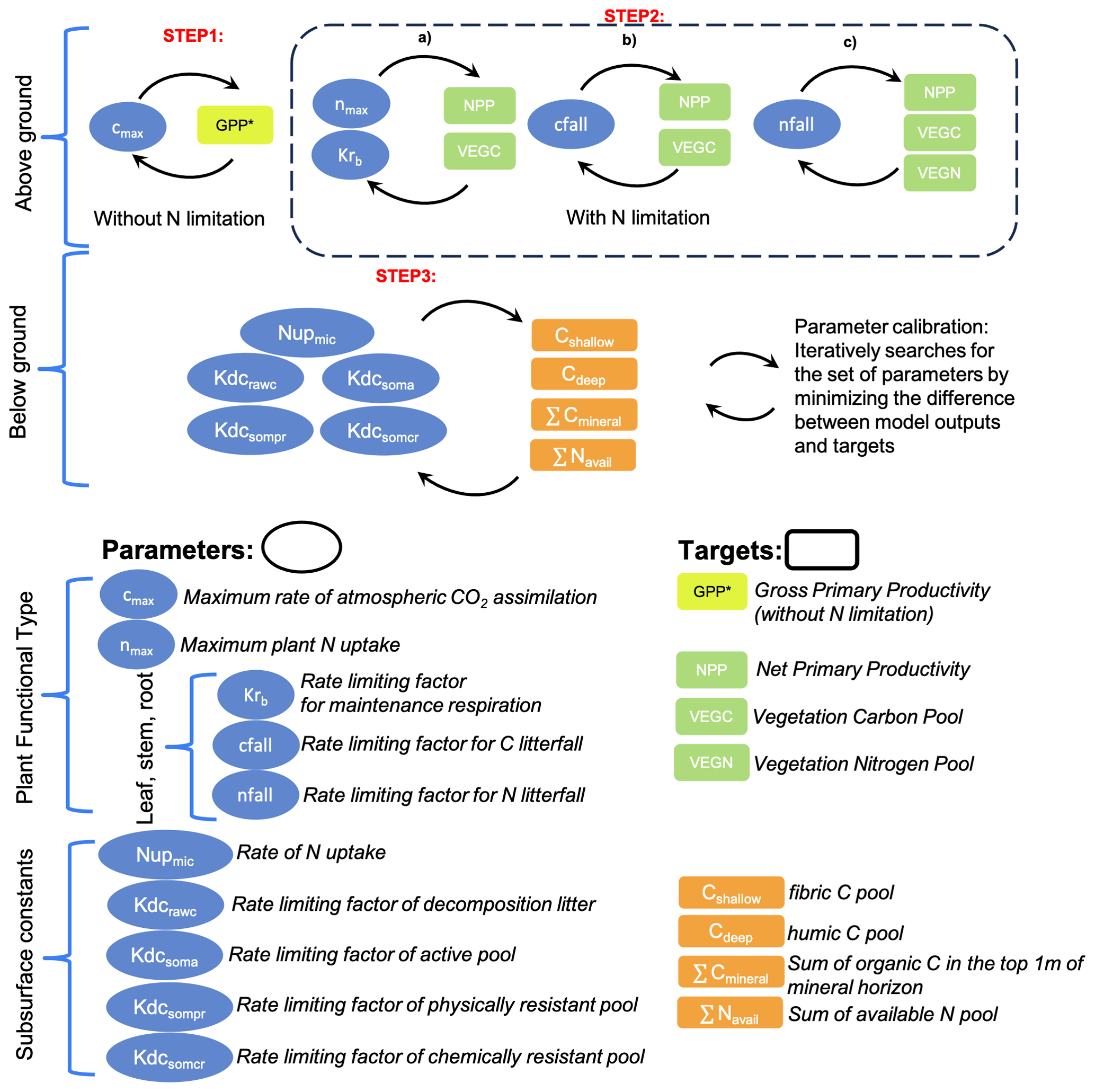
2.6 Calibration process, parameters, and targets

The calibration process in the DVM-DOS-TEM is currently focused on the C and N annual cycles. Thus, calibrated parameters are associated with and adjusted to the major C and N fluxes and stocks in the vegetation and soil. The calibration process follows a hierarchical approach (Fig. 1) in which parameters to be calibrated are organized into hierarchical levels associated with (1) model complexity and feedback and (2) turnover of the processes the parameters are associated with. Therefore, parameters related to vegetation dynamics are calibrated first, followed by the slowest soil-related parameters.

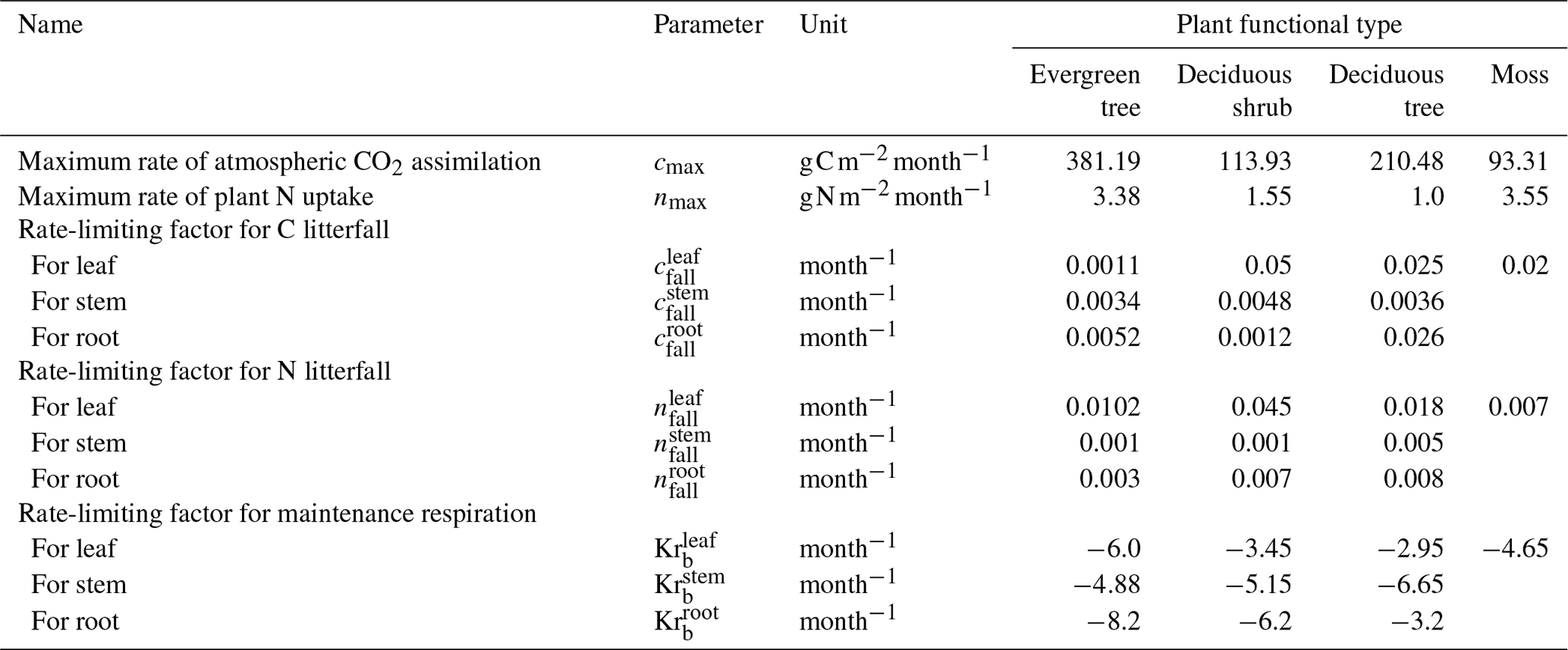
Table 3 Synthetic parameter values for the black spruce forest site used in the parameter calibration process.

The first step of the calibration relates to the simplest and fastest first-order process in the DVM-DOS-TEM and consists of adjusting the rate-limiting parameter of maximum C assimilation of the vegetation (c_max) driving vegetation GPP. In the baseline climate, the main limiting parameter of vegetation productivity in the Arctic is N availability (Chapin and Kedrowski, 1983). Therefore, c_max is calibrated to reproduce estimates of GPP from fertilization experiments where N limitation is ignored (GPP^∗). When fertilization experiments are not available for the community or region of interest, GPP^∗ is estimated by applying a multiplicative factor to the observed GPP under natural conditions. This multiplicative factor is estimated from published fertilization experiments in similar communities and is computed as the ratio between GPP estimated in fertilized plots and GPP estimated in control plots. Based on the literature, this fertilization factor can vary from 1.25 to 1.5 (Ruess et al., 1996; Shaver and Chapin, 1995).

The second step of the calibration process consists of turning on the representation of N limitation on vegetation productivity in the model (Euskirchen et al., 2009) and calibrating the rest of the vegetation-related parameters. In the current workflow, it consists of three substeps. These substeps could follow a different order based on the preference of the user and the specifics of a given site. These are rate-limiting parameters for maintenance respiration (Kr_b), maximum plant N uptake (n_max), and C and N litterfall (c_fall and n_fall, respectively). These parameters are adjusted until DVM-DOS-TEM outputs match observations of GPP and NPP, plant N uptake (Nup), and vegetation C and N pools, respectively. Target values of these variables are listed in Table 1. It is important to note that the parameters Kr_b, c_fall, and n_fall as well as the variables for vegetation C and N are specified per PFT and compartment (leaf, stem, and root).

In the third step, the rate-limiting parameters of soil heterotrophic respiration (kdc) and the rate of microbial N uptake ($n_{\text{micb}}^{\text{up}}$) are calibrated as soil processes and take longer to run in comparison to the first two steps. These parameters are adjusted until the DVM-DOS-TEM outputs match observations of the soil organic C and available N stocks. The target values of these variables are listed in Table 2. In the final step, vegetation-related parameters are checked for a final adjustment after soil calibration, as soil processes can feed back to vegetation dynamics.

2.7 Calibration setup and evaluation metrics

Table 3 shows the parameter values used to calculate synthetic target values. We established four cases by perturbing the parameters by 10 %, 20 %, 50 %, and 90 % from their original values. For each case, the MADS calibration function randomly sampled 10 sets of parameters within the specified ranges. These 10 sets of randomly perturbed parameters were then optimized using the MADS algorithm. For each set of calibrated parameters and targets, we computed the root mean square error (RMSE) and relative error (RE) metrics. RMSE is employed to measure the magnitudes of varying quantities, while RE gauges the absolute difference relative to the actual values. Given that some parameters are small (less than 10⁻³), the relative error provides more informative insights. The following equations were used to compute these metrics:

$$\begin{array}{}\text{(1)}& {\displaystyle }& {\displaystyle }\text{RMSE}=\sqrt{(\stackrel{\mathrm{‾}}{x}-x{)}^{\mathrm{2}}},\text{(2)}& {\displaystyle }& {\displaystyle }\text{RE}=\left|{\displaystyle \frac{\stackrel{\mathrm{‾}}{x}-x}{x}}\right|\cdot \mathrm{100}\mathit{\%},\end{array}$$

where $\stackrel{\mathrm{‾}}{x}$ is the mean of the best 5 out of 10 computed target–parameter matches and x is a synthetic target value.

To ensure the selection of the best-fitting parameters, we sorted the error values from lowest to highest. Then, we selected the top five parameter sets, calculated their mean values, and compared these averaged parameters with the synthetic target values and known parameters.

Table 4 Synthetic below-ground target values for the black spruce forest site used in the parameter calibration process.

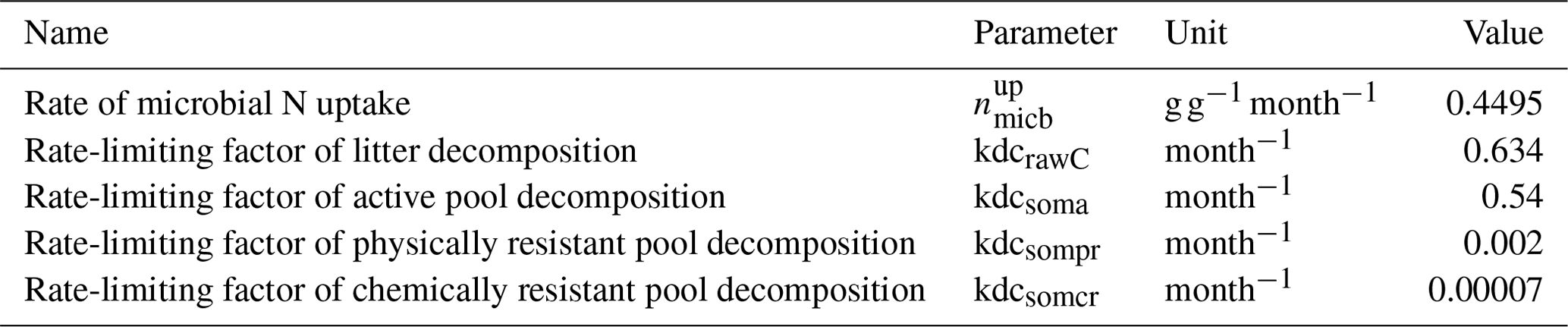
Table 5 Observed vegetation target values at the black spruce forest site used in the parameter calibration process. Standard deviations are indicated in parentheses and are estimated from field measurements (n=15, Melvin et al., 2015).

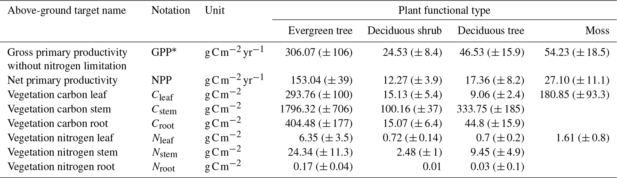
Table 6 Observed below-ground target values at the black spruce forest site used in the parameter calibration process. Standard deviations are indicated in parentheses and are estimated from field measurements (n=15, Melvin et al., 2015).

2.8 Application of the calibration method to observed target values

After validating our calibration method with synthetic data, we applied it to the black spruce site. The observational dataset was compiled using a combination of in situ measurements and values from the existing literature (Tables 5 and 6). Unlike synthetic targets, observed values inherently carry uncertainty, which must be accounted for in the calibration process. The uncertainty range in the observed targets varied from 27 % to 40 % (the maximum coefficient of variation was estimated from observations reported in Melvin et al., 2015), influencing the final calibrated parameter estimates. After calibrating parameters using observed means as targets, we sampled 1000 parameter sets around the calibrated parameter set with a ± 5 % variation for all parameters excluding c_max. This approach was implemented to increase the probability of achieving an optimal match with observations, thereby allowing for a higher set of optimal parameter estimates. Additionally, this process enabled us to evaluate the impact of calibrated soil parameters on vegetation-related target values, which were calibrated over shorter time intervals.

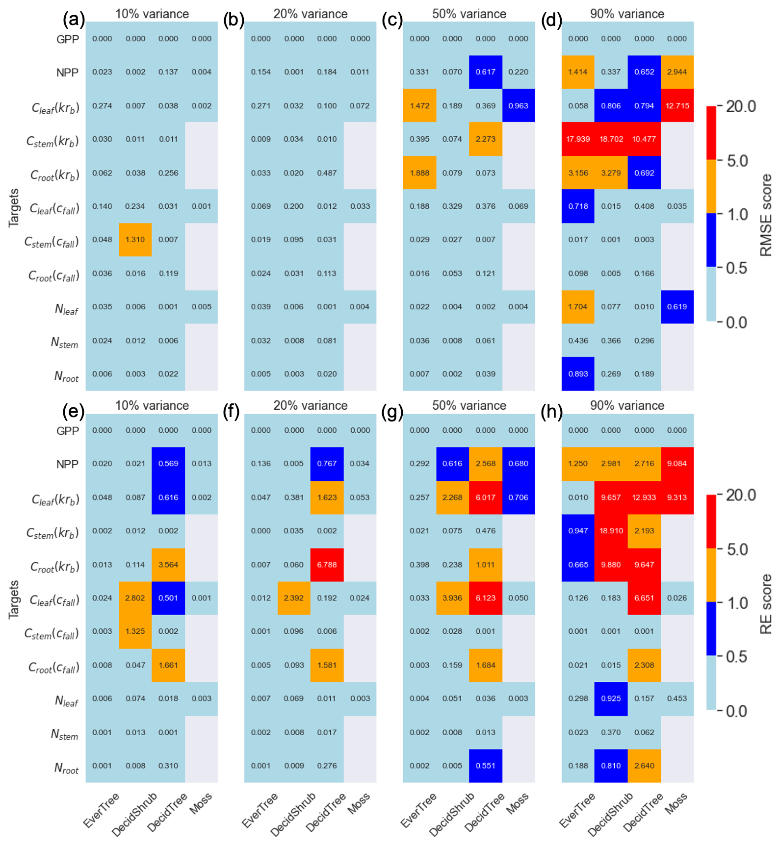
Figure 2 Panels (a–c) and (d) are the root mean square error (RMSE) metric, and panels (e–g) and (h) are the relative error (RE) metrics for the 10 %, 20 %, and 90 % variances in the parameter range. Targets are shown on the y axis, and plant functional types are shown on the x axis. The color bar represents the RMSE and RE scores.

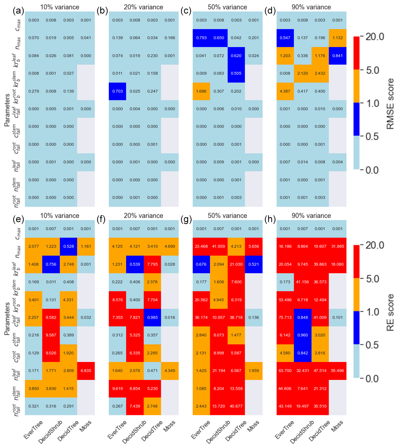
Figure 3 Panels (a–c) and (d) are the RMSE metric, and panels (e–g) and (h) are the RE metrics for the 10 %, 20 %, 50 %, and 90 % variances in the parameter range. The DVM-DOS-TEM parameters are shown on the y axis, and the plant functional types are shown on the x axis. The color bar represents the RMSE and RE scores.

3 Results

3.1 Vegetation targets

Depending on the range of parameter variance, our analysis revealed varying levels of accuracy between known synthetic parameters and those determined using the MADS search approach. In general, the variance between calibrated and synthetic values grew higher with a higher degree of parameter perturbation. The averaged RMSE values for all four PFTs showed similar increases (Fig. 2), with an exception for C_stem(c_fall) deciduous shrubs, which made the RMSE score for the 10 % variance higher than the 20 % variance (Fig. 2a and b). That is why we introduced the RE metric, which shows that the departure between synthetic and calibrated parameters increases with increasing perturbation and is smallest for the 10 % variance (Fig. 3a). Additional analyses for exploring the detailed relationship between the parameter variance and RMSE for specific cases are presented in the Supplement (Figs. S2–S5).

3.2 Vegetation parameters

The RMSE for the parameters was highest for ${\text{Kr}}_{\mathrm{b}}^{\text{root}}$ in the evergreen tree PFT (Fig. 3). Overall, the Kr_b and n_max parameters exhibited the worst recovery compared to other parameters based on the RMSE metric. Conversely, REs were highest for c_fall deciduous shrubs and less so for Kr_b parameters. The RE indicated that smaller parameter values, such as n_fall, deviated more significantly from their synthetic values. Interestingly, the RE score showed the same error range for the 10 % and 20 % variance ranges, whereas the RMSE showed that 10 % variance has the smallest error.

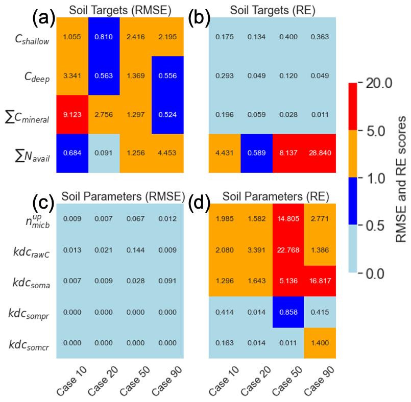
Figure 4 Comparison between calibrated and synthetic subsurface target value (a) RMSE and (b) RE scores. Comparison between calibrated and synthetic subsurface parameter value (c) RMSE and (d) RE scores for all range variances. The color bar represents the RMSE and RE scores.

3.3 Soil parameters

In general, the RMSE values for the subsurface target parameters were relatively small but increased with a higher variance range (Fig. 4). Notably, C_deep and ∑C_mineral exhibited high RMSE values of 3.34 and 9.12, respectively, for the 10 % variance range (Fig. 4a). Despite this, the soil parameters for 10 % variance showed the best match, with RMSE values of less than 0.01. The RE for the targets revealed increasing deviations from the synthetic parameter values for ∑N_avail. The RE for the parameters indicated that $n_{\text{micb}}^{\text{up}}$, kdc_rawC, and kdc_soma had higher deviations from their respective synthetic values for the 50 % and 90 % variance ranges.

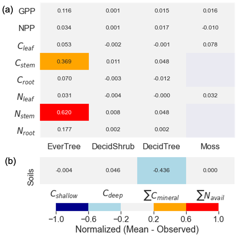
Figure 5 The comparison between the observed and calibrated target values. The target values are shown on the y axis, and the plant functional types (a) and soil targets (b) are shown on the x axis. The color bar represents the difference between the normalized modeled and observed target values.

3.4 Comparison with observations

Figure 5 shows a comparison between observed and modeled target values after calibration. Both observed and modeled values were normalized by dividing by the highest value within their respective groups (e.g., GPP or NPP). The highest difference (exceeding 20 % uncertainty) was observed for evergreen trees (black spruce). Notably, we encountered challenges in accurately matching the values of the C_stem target and the values of N_stem (Fig. 5a). Additionally, while the calibration method struggled to align the carbon in the soil mineral pool, it captured other soil target values (Fig. 5a). Overall, the results demonstrate that the calibration approach is effective and reliable for optimizing DVM-DOS-TEM parameters.

4 Discussion

Our findings highlight the challenges associated with calibrating carbon and nitrogen dynamics in high-latitude permafrost ecosystems and, particularly, accurately estimating carbon pools with slow turnover of deep-mineral soil carbon and allocation of carbon and nitrogen resources within vegetation compartments in order to match observations closely. The strong interdependencies between parameters and state variable target values underscore the complexities of process-based modeling, reinforcing the need for automated calibration approaches like MADS to improve predictive accuracy.

4.1 Importance of the initial parameter guess

The initial parameter values, or initial guess, had minimal impact on the synthetic experiment, as the perturbed parameters were sufficiently close to the true values. However, for non-synthetic calibrations, the initial state is crucial, as starting with parameter values far from the true state can lead to non-convergence and significantly increase computation time (Nocedal and Wright, 2006). To address this, we developed parameter sensitivity methods to improve initial estimates (Briones et al., 2024). This approach utilized ensemble model simulations executed in parallel, systematically exploring parameter ranges through Latin hypercube sampling or uniform random sampling. By employing parallel processing before integrating parameters into the MADS calibration framework, we effectively refined initial estimates, minimized deviations from target values, and improved the overall calibration efficiency.

4.2 Analysis of the recovery metrics

The mean parameter values calculated from the five best-matched MADS value predictions align closely with the synthetic parameter values, demonstrating the method's efficacy. The calculated REs for the parameters indicate that the relative distance between the calibrated and synthetic values increases with a higher parameter variance range, except for REs for soil targets (Fig. 4b, 20 % case). For the soil targets, the RMSE for ∑N_avail for the 10 % variance range was higher than that of the 20 % variance range. The higher RMSE for the 10 % variance range than for the 20 % variance range for vegetation-related targets and soil targets could be due to the limited number of cases (n=10) in each variance range. It is highly probable that increasing the total number of searches (higher than 10) would yield a more consistent pattern of decreasing accuracy with increasing variance.

4.3 Parameter–target relationship and small parameter values

The method demonstrated robust recovery of c_max values, indicating that it performs best when there is a linear relationship between parameters and target values (Eq. S1). For parameters that do not exhibit a linear relationship with their target values (e.g., Kr_b, Eq. S4), the calibrated parameters showed wider variance. Additionally, small parameter values, such as n_fall, corresponded to a small range of sampled values, leading to insensitivity between n_fall and vegetation N. To address this, we applied a logarithmic transformation to these and some other small values for soil C rates.

4.4 The impact of n_max on N uptake and NPP

Sensitivity between model parameters and targets is crucial for effective parameter calibration. We observed that the sensitivity between n_max and NPP was not strong (Eqs. S2 and S5), which led us to combine its calibration with the Kr_b parameter. Based on Eq. (S2), n_max directly influences N_uptake. An increase in n_max enhances N_uptake, thereby increasing the total N supply. Since NPP is proportional to N_supply and inversely proportional to N_required, a higher N supply can lead to a higher NPP, provided that other factors remain constant. Therefore, despite the initial observation of weak sensitivity, n_max could have a considerable impact on NPP due to its role in N_uptake and the overall N_supply. However, our target values for plant N uptake are poorly constrained due to a lack of sufficient observations. This underestimation of plant N uptake could account for the observed lack of sensitivity of NPP to n_max. This issue requires further investigation and currently underscores the importance of accurately calibrating n_max to ensure better simulation of ecosystem productivity.

4.5 The calibration workflow

Our findings indicate that calibrating one or two parameter sets at a time, while keeping other parameters constant, is more effective than calibrating all parameters simultaneously. In the current workflow, we combined n_max and Kr_b (Fig. 1, Step a), which was based on the low sensitivity of n_max to NPP. Combining multiple variables in one calibration step increases the computation time and could result in low match accuracy. On the other hand, sequential parameter calibration carries the risk of losing accuracy for parameters calibrated in previous steps. To mitigate this risk, we include targets from previous calibration steps in the current calibration step. For example, when optimizing for n_fall, we include targets for NPP, vegetation C, and vegetation N.

Sequentially calibrating individual parameter sets is advantageous not only computationally, but also in preventing the occurrence of underdetermined problems, which arise when the number of parameters exceeds the number of targets. Undetermined problems exhibit a lower rate of convergence due to the correlation between parameters and the sensitivity of multiple parameters to one or a few similar target values. The study by Jafarov et al. (2020) showed that overdetermined problems with a higher and diverse number of target values are more effective in recovering accurate parameter values.

4.6 Sensitivity of the Kr_b parameter to NPP and vegetation C

The Kr_b parameter exhibited higher sensitivity to both NPP and vegetation C compared to other parameters. Despite the overall good model fitness, the deviation from the synthetic values for Kr_b was higher. This was primarily due to the ${\text{Kr}}_{\mathrm{b}}^{\text{root}}$ parameter for evergreen trees (Fig. S3C) persistently showing a higher discrepancy. Its sensitivity can be explained by examining its role in the equations governing maintenance respiration (R_m, Eq. S3). The relationship between biomass and maintenance respiration is nonlinear; R_m increases as biomass increases, where Kr_b controls the intercept of this relationship (Tian et al., 1999). Since NPP is computed as a result of GPP and autotrophic respiration, including R_m, any alteration in Kr_b impacts NPP directly (Eq. S9). This sensitivity underscores the importance of accurately calibrating Kr_b to ensure the correct simulation of ecosystem productivity and C dynamics in the DVM-DOS-TEM.

4.7 Vegetation and below-ground C stock equilibrium time

Due to faster turnover, vegetation C and N stocks and fluxes equilibrate faster than soil C and N stocks and fluxes. Thus, we used a two-phase equilibration approach: 200 years for the vegetation and 2000 years for the soil. However, the C stocks achieved after 200 years of equilibration for vegetation might shift when the model is run for an additional 1800 years to equilibrate soil. To mitigate this issue, we developed equilibrium checks to ensure that the vegetation stocks remain stable and close to their equilibrium values throughout the extended simulation period required for soil stock equilibration. These checks help identify significant departures from the initial equilibrium values of vegetation C and N while allowing the model to run for a longer duration to achieve below-ground equilibrium. This approach ensures the accuracy and stability of both vegetation and below-ground C and N stocks in long-term model simulations.

Reversing the calibration sequence and starting from soil parameters is not only impractical in the context of our model but is also computationally inefficient. Vegetation-related parameters are calibrated first because vegetation carbon pools reach equilibrium significantly faster than soil carbon pools, whereas soil pools require longer timescales to stabilize. Beginning with soil parameters would thus introduce unnecessary complexity and substantially increase the total computational cost of the calibration process. In addition, while the choice of calibration sequence may lead to slight variations in the final parameter estimates, our results demonstrate that the proposed “hierarchical approach” (breaking the parameter sets into smaller subsets) effectively recovers parameter values, even when this is for the 90 % parameter range variance. As we showed in this study, well-calibrated parameters exhibit a narrow range of uncertainty, reinforcing the robustness of the method.

4.8 Observed target values

The results of parameter calibration using site-specific observations indicate challenges in accurately matching C_stem and N_stem target values for the evergreen plant functional type. This discrepancy could be related to the allocation scheme of the model, attributing NPP resources to the various compartments of the plant (Fox et al., 2018). Additionally, the model struggled to maintain the assigned carbon value for ∑C_mineral. The difficulty in calibrating C_stem(E) and C_root(E) for evergreen trees can be partially attributed to strong parameter interdependencies (see Figs. S7–S10). For instance, ${\text{Kr}}_{\mathrm{b}}^{\text{leaf(E)}}$ exhibits simultaneous correlations with both C_stem(E) and C_root(E) (Fig. S7), while $c_{\text{fall}}^{\text{stem(E)}}$ shows an inverse correlation with N leaves, stems, and roots (Fig. S8). These multi-target dependencies introduce additional complexity, making it challenging to achieve a precise match for individual target values.

Similarly, the ∑C_mineral target value is strongly influenced by kdc_soma and kdc_sompr, both of which exert substantial control over C_deep and ∑N_avail target values. These interactions underscore the systemic constraints imposed by parameter interdependencies. Furthermore, this discrepancy could be related to the functions controlling vertical transfers of carbon between horizons and the vertical distribution of carbon quality (Harden et al., 2012). The model consistently showed that longer equilibration times lead to a reduction in the mineral soil carbon pool. This was also observed by Schaefer and Jafarov (2016) in a different process-based ecosystem model, where they addressed the issue by incorporating substrate availability constraints to prevent long-term carbon loss. Given the complexity of these interdependencies, further investigation is needed, though this goes beyond the scope of this study.

The calibration of rate-limiting soil parameters that influence C and N stocks and turnover directly impacts vegetation productivity by modulating nitrogen availability. Figure S10 shows a significant correlation between microbial nitrogen uptake and the C_leaf(DS) of deciduous shrub, highlighting the interaction between soil processes and vegetation-related parameters. While long-term soil parameter calibration inherently feeds back into vegetation dynamics, the most substantial changes in vegetation-related parameters typically occur during short-term model runs, resulting in minimal net changes over extended simulations.

4.9 Limitations

There are cases where the model fails to accurately match target values due to poor data quality or its inability to fully represent certain ecological processes (Dietze et al., 2018; Luo et al., 2016). Large discrepancies between observed and modeled targets can hinder the convergence of the LM method, requiring more iterations and leading to suboptimal agreement with observations. As mentioned previously, starting with well-constrained initial parameter estimates can mitigate this issue, which can be achieved by performing sensitivity analyses to identify the most influential parameters and refine their ranges prior to calibration (Efstratiadis and Koutsoyiannis, 2010).

Additionally, calibrating soil-related parameters is computationally demanding, often resulting in a substantial slowdown of the overall calibration workflow. Machine learning (ML) models offer a promising solution by acting as surrogate models to approximate the equilibrium state, thereby reducing the computational burden (Fer et al., 2018; Reichstein et al., 2019). However, implementing such approaches necessitates large training datasets, often requiring thousands of model simulations to achieve reliable predictions. Future research should explore the integration of ML-based calibration techniques into the workflow, which could significantly enhance computational efficiency and further improve model accuracy (Castelletti et al., 2012; Dagon et al., 2020).

5 Conclusion

In this study, we showed that the developed MADS parameter calibration method for the DVM-DOS-TEM can effectively recover the synthetic parameter set, optimizing labor and time and enhancing the reproducibility of the calibration process. By implementing a structured workflow that calibrates one or two parameters at a time and includes equilibrium checks, the method ensured accurate parameter estimation even for a high-variance parameter range. The primary advantage of the semi-automated MADS calibration approach is its significant enhancement of repeatability and clear quantification of calibration performance. In contrast, manual calibration processes are often difficult to reproduce, as it is impractical if not impossible to record users' continuous adjustments to parameter values until improved results are achieved. Additionally, appreciation of model improvement by a user is often subjective, as running a statistical evaluation of each parameter adjustment would be too time-consuming. In the approach demonstrated in this study, we introduced a calibration metric that provides a quantifiable measure of the overall quality of the calibration. This metric enhances reproducibility by allowing future users working at the same site to follow the established workflow and reliably reproduce the calibrated parameter and target values. The RMSE quantifies the average differences between calibrated and observed (synthetic) values, while the RE metric indicates deviations from the synthetic values.

In all of the calibration experiments, we utilized only 10 randomly perturbed initial parameter sets within a specified variance range. Our results indicated that perturbation ranges of 10 %–20 % were equally effective in achieving optimal target–parameter calibration. However, increasing the number of random perturbations could potentially shift the statistics, favoring a 10 % variance range.

While the choice of the initial guess is crucial, its impact was mitigated in our study due to the design involving variance around synthetic parameter values. The developed method significantly reduces the labor and time required for calibrating DVM-DOS-TEM parameters. However, it does not entirely replace the need for human intervention. Users still need to understand the specifics of the model and the relationship between parameters and targets, and they need to conduct postprocessing assessments of the fit. In future work, we will apply this method to data processed at multiple study sites to validate the calibration approach further and refine it.

The application of the calibration method to site-specific observations revealed challenges in accurately matching C_stem, N_stem, and ∑C_mineral values, primarily due to parameter interdependencies and data uncertainties. Discrepancies between observed and modeled target values exceeded the known measurement uncertainty, suggesting that structural uncertainty within the model may contribute to these deviations. This indicates a potential need for a more detailed representation of ecological processes to improve model accuracy. However, these challenges may be site-specific and may not necessarily apply to other ecosystem types. Despite these limitations, the study demonstrates the effectiveness and reliability of the calibration approach while identifying key areas for future model refinement.