The sensitivity of aerosol data assimilation to vertical profiles: case study of dust storm assimilation with LOTOS-EUROS v2.2

Modelling and observational techniques are pivotal in aerosol research, yet each approach exhibits inherent limitations. Aerosol observation is constrained by its limited spatial and temporal coverage compared to that of models. On the other hand, models tend to possess higher uncertainties and biases compared to observations. Aerosol data assimilation has gained popularity as it combines the advantages of both methods. Despite numerous studies in this domain, few have addressed the challenges faced in assimilating aerosol data with significant differences in magnitude and degree of freedom between the model state and observations, especially in the vertical direction. These challenges can lead to the preservation – or even the exacerbation – of structural inaccuracies within the assimilation process. This study investigates the sensitivity of dust aerosol data assimilation to the vertical structure of the aerosol profile. We assimilate a variety of dust observations, encompassing ground-based particulate matter (PM₁₀) measurements, and satellite-derived dust optical depth (DOD) data, using the ensemble Kalman filter (EnKF). The assimilation process is elucidated, detailing the assimilation of raw ground-based and satellite-based observations for an optimized three-dimensional (3D) posterior state. To demonstrate the impact of accurate vs. erroneous prior aerosol vertical profiles on the assimilation result, we select three cases of super dust storms for analysis. Our findings reveal that the assimilation of ground observations would optimize the dust field at the ground in general. However, the vertical structure presents a more complex challenge. When the prior profile accurately reflects the true vertical structure, the assimilation process can successfully preserve this structure. Conversely, if the prior profile introduces an incorrect structure, the assimilation can significantly deteriorate the integrity of the aerosol profile. This is also found in the assimilation of DOD, which exhibits a comparable pattern in its sensitivity to the initial aerosol profile's accuracy.

1 Introduction

In recent decades, atmospheric aerosol has garnered extensive attention due to its impact on the environment (Buseck and Pósfai, 1999; Zhao et al., 2020) and human health (Zhu et al., 2021). Numerous research studies have been conducted on the characterization (Mhawish et al., 2021), source apportionment (Wu et al., 2018), and model simulation (Lee et al., 2011) of aerosols. One crucial tool for understanding aerosol processes and forecasting is the chemical transport model (CTM), which can generate continuous three-dimensional (3D) aerosol fields on a large scale. However, despite significant efforts to develop and improve CTM parameter schemes, studies have pointed out that significant uncertainties still exist in CTM simulations (Vignati et al., 2010; Stier et al., 2013). These uncertainties primarily arise from emission sources (e.g. intensity, location), meteorological inputs (e.g. wind mixing, precipitation), and incomplete parameter schemes (e.g. chemical reactions) (Benedetti et al., 2018). At the same time, aerosol measurements have advanced, owing to the development of sensors and increased investment. These include chemical kinetics studies in laboratories (Kolb and Worsnop, 2012), a network of loosely distributed ground monitoring stations (Gueymard and Yang, 2020), and regularly scanning satellites providing global coverage (Sogacheva et al., 2020). Although these measurements offer higher accuracy, challenges persist. So far, obtaining continuous 3D aerosol measurements on a large scale remains impractical and costly. Measurements are limited to surface-level concentrations of total particle matter, column-integrated aerosol optical depths (AODs), and vertical profiles of total aerosol extinction. These measurements have fewer degrees of freedom compared to the complexity of reality (Pappalardo et al., 2014; Qin et al., 2021).

Data assimilation incorporates models and measurements to generate a posterior that holds the strengths of both (Bannister, 2017). Various data assimilation techniques have been developed for different applications, including hydrology (Reichle et al., 2002), geology (Peng and Liu, 2022), and atmospheric science (Hamill, 2006). These methods are typically based on either variational or ensemble approaches (Whitaker et al., 2009; Law and Stuart, 2012). The variational method is particularly useful for emission inversion (Bergamaschi et al., 2022; Jin et al., 2023a). Ensemble-based filters have also demonstrated superior performance in sequential forecasting without the adjoint or tangent linear model required by the variational method. By assimilating real-time observations, these filters generate optimized initial fields that enhance forecast accuracy (Houtekamer et al., 2005). Since the introduction of the classic ensemble Kalman filter (EnKF) (Evensen, 1994), a considerable amount of research has focused on its application and improvement. Several variations of the EnKF, such as EnSRF (Whitaker and Hamill, 2002) and LETKF (Hunt et al., 2007), have been proposed to address computational complexity, accuracy, and robustness issues. Although these advancements have been validated, challenges related to the model's background error covariance and observational data quality control can still impact the assimilation results significantly.

In data assimilation methodology, an observation operator is required for deriving the innovation vector that quantifies the difference between the observation field and the simulation field (Ma et al., 2020). These two usually have different degrees of freedom. With that, the optimized state could then be calculated considering the integration of background and observational penalties. From the perspective of aerosol data assimilation, the main objective is to reproduce optimal aerosol states (Liu et al., 2011), considering their spatial, vertical, aerosol species, and size distribution characteristics, while currently available observations commonly measure their mixed state. For example, AOD is the column-integrated optical extinction of all aerosols, and high uncertainties exist in the optical properties of aerosol (Tsikerdekis et al., 2021). Ground PM₁₀ concentration measurement is the additive sum of all particles with a diameter less than 10 µm. The ground PM₁₀ measurements are not directly comparable to the aerosol state. For ground measurements, monitoring stations are sparsely distributed, making high data vacancy in AOD products inevitable as a result of retrieval failures. The number of observations is therefore commonly much lower than the model state, or the degree of freedom is limited compared to that of the model state. Mathematically, the assimilation result strongly depends on the background error covariance for transferring the increments from the low-degree observational space to the full model space. Given a partially erroneous prior, the assumptions about the prior states can be reserved – or even exacerbated – with the lack of observations. Only a few studies have focused on some of these aspects. We recently found that the incorrect assumption of aerosol size distribution from prior models gives rise to a worse posterior (Jin et al., 2023b). In addition, the position error in the dust plume simulation can lead to the failure of assimilating valid observations (Jin et al., 2021). With regard to the vertical structure, most studies have focused on proposing relevant assimilation methods to assimilate observations, such as the Cloud-Aerosol Lidar with Orthogonal Polarization (CALIPSO) (Sekiyama et al., 2010; Cheng et al., 2019; Ye et al., 2021) and light detection and ranging (lidar) (Wang et al., 2022). The sensitivities of assumptions in the prior simulations need to be explored.

For example, in dust aerosol data assimilation, the most representative observation sources are direct observations, like PM₁₀ and PM_2.5 concentrations, and indirect observations, like dust optical depth (DOD) and extinction coefficient (Jin et al., 2022). Since they are all a combination of different particles, it is necessary to perform bias correction before assimilation (Jin et al., 2019; Ma et al., 2020). Afterwards, through assimilation analysis, few observations can optimize the whole model state space, while in reality, ground stations produce scattered concentrations on the ground, and satellites and lidars receive column-integrated information about the aerosol or a single profile once a day (Sekiyama et al., 2010; Hofer et al., 2017; Cheng et al., 2019; Escribano et al., 2022). None of them can provide continuous vertical information about the aerosol with large spatial coverage. When there is incorrect information about the dust aerosol structure in the model prior, due to the considerably greater degree of freedom of the model state, data assimilation algorithms may fail to correct it or, even worse, further degrade the vertical dust aerosol loading.

There is limited research addressing the impact of flawed aerosol prior assumptions on the degradation of the assimilated posterior, particularly concerning vertical structures. Gwyther et al. (2023) delved into the implications of 4DVar data assimilation for mesoscale eddy representation in the vertical dimension, highlighting that inadequate prior knowledge of these structures significantly hinders improvement in the assimilated simulations. This issue extends to aerosol data assimilation, where erroneous assumptions regarding aerosol vertical distribution cause assimilation methods to maintain or exacerbate inaccuracies. This study focuses on several major dust storm events that occurred in the spring of 2021, utilizing them as case studies. We conduct separate data assimilation experiments involving ground-level PM₁₀ measurements and satellite-based AOD data to demonstrate explicitly how misleading vertical prior information can distort the posterior results. The LOTOS-EUROS model facilitates the reproduction of dust dynamics and generates the initial dust load priors. For assimilation, we employ an EnKF algorithm, incorporating bias-corrected PM₁₀ data from ground stations and DOD retrievals from the Himawari-8 satellite. For validation, we employ aerosol profile observations from CALIPSO and lidar systems. By presenting both favourable and detrimental scenarios, this work underscores the high sensitivity of data assimilation processes to the accuracy of assumed vertical structures, thereby emphasizing the criticality of precise vertical profiling in aerosol studies.

The remainder is organized as follows. Section 2 describes the model used for the dust aerosol simulation and the dust observations used in this study. Section 3 introduces the assimilation algorithm applied to assimilate the observations and the experiment settings. Section 4 discusses the assimilation results and validates the results with the CALIPSO and lidar observations. Finally, Sect. 5 summarizes the study.

2 Dust aerosol simulation and observations

This section introduces the model used for simulating dust aerosol and describes the observation methods applied for monitoring dust, including a ground monitoring station, Himawari-8, CALIPSO, and lidar. Among these, ground PM₁₀ from ground monitoring stations and DOD from Himawari-8 are used for assimilation. Extinction profiles from CALIPSO and lidar are used to validate the posterior profile.

2.1 Dust simulation

2.2 LOTOS-EUROS

LOTOS-EUROS v2.2 is used to simulate the dust aerosol. The LOTOS-EUROS model is a 3D chemistry transport model used for air quality forecasting (Manders et al., 2017). It has also been applied in source apportionment and emission inversion worldwide. In this study, the modelling domain spans 15 to 50° N and 70 to 140° E with a spatial resolution of 0.25°×0.25°. Vertically, it comprises 21 layers with a top level at 10 km, which is adequate for recognizing the vertical structure. An ECMWF operational forecast of 3 h is used to drive the model. The boundary conditions are set to zero assuming that all the dust aerosols are emitted during the simulation window. Dust aerosol processes, including emission, advection, diffusion, deposition, and sedimentation, are considered in the model.

All simulations commence 1 d prior to the initial assimilation time point, during which no dust emission occurs. The dust emission process is modelled using the Zender03 emission parameterization scheme (Zender et al., 2003). In general, we assign the dust simulation uncertainty to the dust emission. Ensemble emission fields $[{\mathit{f}}_{\mathrm{1}},\mathrm{\dots },{\mathit{f}}_N]$ are generated randomly following the emission uncertainty choice f_priori and background error covariance matrices B in Jin et al. (2022). They are used to forward the LOTOS-EUROS model ℳ for the ensemble dust simulations $[{\mathit{x}}_{\mathrm{1}},\mathrm{\dots },{\mathit{x}}_N]$ as

$$\begin{array}{}\text{(1)}& {\displaystyle }{\displaystyle }[{\mathit{x}}_{\mathrm{1}},\mathrm{\cdots },{\mathit{x}}_{\mathit{N}}]=\left[\mathcal{M}\right({\mathit{f}}_{\mathrm{1}}),\mathrm{\cdots },\mathcal{M}({\mathit{f}}_N\left)\right].\end{array}$$

Here, N refers to the total ensemble number.

2.3 Dust observations for assimilation

2.3.1 Ground PM₁₀

There are over 1600 ground air quality monitoring stations located throughout China. Their spatial distribution can be seen in Fig. 1 (blue scatters). They provide hourly air pollutant concentrations, including PM_2.5, PM₁₀, O₃, NO₂, SO₂, and CO. PM₁₀ can appropriately represent the dust load as it falls under the size definition of fine and coarse dust (Adebiyi et al., 2023). Its uncertainty is also relatively lower than that of some remote sensing instruments. However, PM₁₀ is a combination of various species. Assimilating such observations with inaccurate or incorrect representativeness can diverge the model. It is then necessary to perform bias correction (BC) to remove the non-dust parts before they are assimilated. Details concerning the method can be found in Jin et al. (2022). The bias-corrected observations can be used to correct the model simulation by data assimilation.

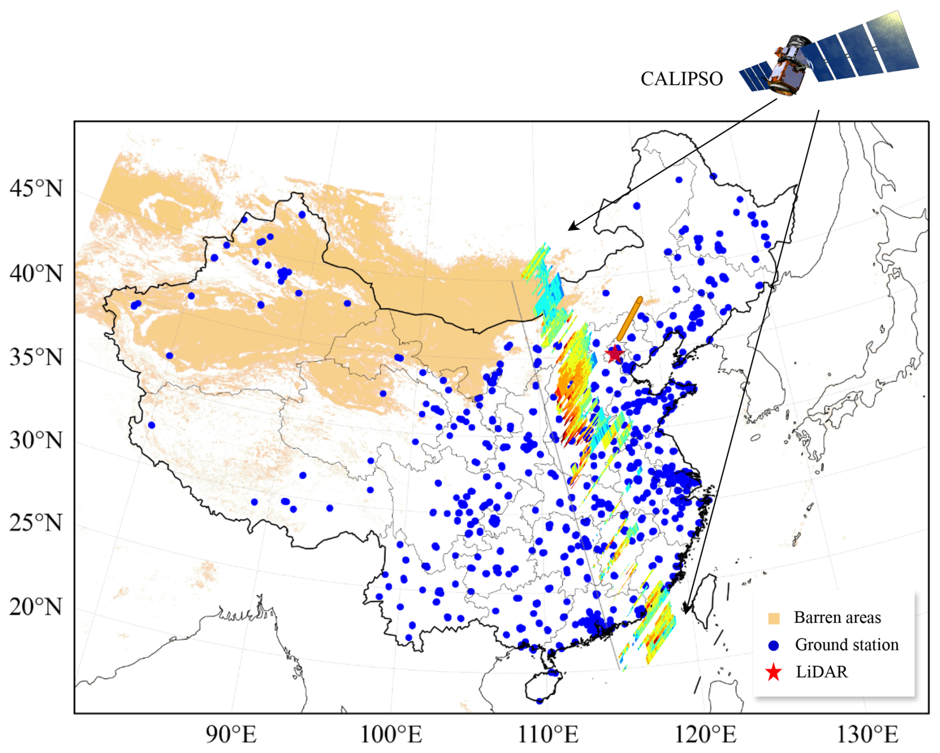
Figure 1 Spatial distribution of ground monitoring stations (blue scatters), location of the lidar (red star) with upward-scanning ray (orange cylinder), and aerosol extinction profile sample scanned by the CALIPSO satellite (trajectory is plotted as the grey line on the ground).

2.3.2 Himawari-8 AOD and calculation of DOD

The Himawari-8 geostationary satellite, operated by the Japan Meteorological Agency (JMA), provides aerosol optical information covering East Asia and the western Pacific region at a time resolution of 10 min (Yumimoto et al., 2016). This allows us to monitor the source and movement of dust at high spatial–temporal resolution. Its products, the Ångström exponent ($\stackrel{\mathrm{˚}}{A}$) and aerosol optical thickness (AOT) at 550 nm, are selected to measure the dust optical depth (DOD). These data are merged to model grid (0.25°×0.25°) and hourly resolution.

To remove the fine-mode non-dust AOD in total AOD, an empirical function concerning $\stackrel{\mathrm{˚}}{A}$ is used to calculate the submicron fraction (SMF) (Anderson et al., 2005; Di Tomaso et al., 2022). The dust optical depth (DOD) can then be obtained by the SMF.

$$\begin{array}{}\text{(2)}& {\displaystyle }& {\displaystyle }\text{SMF}=-\mathrm{0.0512}\times {\stackrel{\mathrm{˚}}{A}}^{\mathrm{2}}+\mathrm{0.5089}\times \stackrel{\mathrm{˚}}{A}+\mathrm{0.02}\text{(3)}& {\displaystyle }& {\displaystyle }\text{DOD}=\text{AOD}\times (\mathrm{1}-\text{SMF})\end{array}$$

Furthermore, the threshold of $\stackrel{\mathrm{˚}}{A}\le \mathrm{1}$ is set to exclude the fine-mode dominant observations.

2.4 Dust observations for validation

The aerosol extinction coefficient from CALIPSO and lidar is used to validate the vertical structure of dust aerosol.

2.4.1 CALIPSO

The Cloud-Aerosol Lidar with Orthogonal Polarization (CALIOP), on board the CALIPSO satellite, provides data on the vertical structures and types of aerosols on a global scale (Winker et al., 2010). It has a spatial resolution of 333 m and a vertical resolution of 30 m. A normal extinction profile sample can be seen above the dashed black line in Fig. 1a. It has been widely used in investigating aerosol distribution and evolution (Xu et al., 2020; Zhang et al., 2020; Han et al., 2022; Chen et al., 2023) and data assimilation (Sekiyama et al., 2010; Cheng et al., 2019; Escribano et al., 2022). Here, its product, extinction coefficient at 532 nm, is taken as the aerosol profile validation set to identify the vertical distribution of the dust load.

2.4.2 Polarization lidar

Polarization lidar deployed on the ground can provide continuous measurements on the vertical details of the atmospheric environment with high resolution (Hofer et al., 2017). Recently, Wang et al. (2021) collected dust extinction coefficient data through a dual-wavelength aerosol lidar built in the tower of the Institute of Atmospheric Physics (39°58^′35^′′ N, 116°22^′41^′′ E; red star in Fig. 1a). The device provided dust information with a high vertical resolution of 30 m and temporal resolution of 15 min. The vertical profile development of the several super dust storms that occurred in the spring of 2021 was thoroughly captured by the instrument, thus making it a crucial source of measurement for learning about the vertical structure and its development during dust storms. In this study, these data are employed to compare the vertical structures from the model simulation and assimilation analysis.

3 Assimilation methodology and experiments

This section first illustrates the methodology of the classic EnKF used in Sect. 3.1. The sensitivity of the aerosol posterior to the vertical structure is then emphasized when assimilating the ground PM₁₀ concentrations in Sect. 3.2 and the DOD in Sect. 3.3. Case experiments evaluating this sensitivity are described in Sect. 3.4.

3.1 EnKF

The data assimilation algorithm used in this study is the stochastic EnKF formulated by Burgers et al. (1998). It is implemented in our self-developed PyFilter toolbox (Pang, 2024). Its capability to improve dust forecasting has been proven in our recent research (Pang et al., 2023). We did not adopt any other variant of EnKF because the problem we address is contingent but universal in aerosol data assimilation applications.

EnKF is a Monte Carlo approach based on Kalman filter theory. EnKF maintains a set of model states to approximate the probability distribution of the model state or parameter. It includes the forecast step and the analysis step. In the forecast step, each posterior ensemble member ${\mathit{x}}_{t-\mathrm{1}}^{a,i}$ at the previous time t−1 is integrated forward according to the model dynamics ℳ to generate a prior forecast ${\mathit{x}}_t^{f,i}$ at the next moment t. Here, i refers to the ensemble member.

$$\begin{array}{}\text{(4)}& {\displaystyle }{\displaystyle }{\mathit{x}}_t^{f,i}=\mathcal{M}\left({\mathit{x}}_{t-\mathrm{1}}^{a,i}\right)\end{array}$$

In the analysis step, the states of each member are adjusted based on observational data to approach the true state. This adjustment process is implemented based on the error from the model prior and observation. In EnKF, the model prior error covariance matrix P^f is calculated through the ensemble approximation method following

$$\begin{array}{}\text{(5)}& {\displaystyle }{\displaystyle }{\mathbf{P}}^f={\displaystyle \frac{\mathrm{1}}{N-\mathrm{1}}}({\mathit{x}}_i^f-{\stackrel{\mathrm{‾}}{\mathit{x}}}^f)({\mathit{x}}_i^f-{\stackrel{\mathrm{‾}}{\mathit{x}}}^f{)}^{\mathrm{T}},\end{array}$$

where N is the number of ensembles, ${\mathit{x}}_i^f$ is the ith individual of the ensemble prior states, and ${\stackrel{\mathrm{‾}}{\mathit{x}}}^f$ is the average of the ensemble members.

Then, a weight matrix K, also referred to as the Kalman gain, can be obtained by

$$\begin{array}{}\text{(6)}& {\displaystyle }{\displaystyle }\mathbf{K}={\mathbf{P}}^f{\mathcal{H}}^{\mathrm{T}}(\mathcal{H}{\mathbf{P}}^f{\mathcal{H}}^{\mathrm{T}}+\mathbf{R}{)}^{-\mathrm{1}}.\end{array}$$

The a posteriori ensemble individual ${\mathit{x}}_i^a$ is calculated by

$$\begin{array}{}\text{(7)}& {\displaystyle }{\displaystyle }{\mathit{x}}_i^a={\mathit{x}}_i^f+\mathbf{K}(\mathit{y}+{\mathit{ϵ}}_i-\mathcal{H}{\mathit{x}}_i^f),\end{array}$$

where ϵ_i is the extra perturbation, and its variance is set according to the diagonal of the observation error covariance R. It serves to maintain the ensemble spread (van Leeuwen, 2020).

Meanwhile, the a posteriori x^a can be updated via

$$\begin{array}{}\text{(8)}& {\displaystyle }{\displaystyle }{\mathit{x}}^a={\stackrel{\mathrm{‾}}{\mathit{x}}}^f+\mathbf{K}(\mathit{y}-\mathcal{H}{\stackrel{\mathrm{‾}}{\mathit{x}}}^f).\end{array}$$

From the equations above, we can tell that the a posteriori is dependent on both the prior and the observations. Within different spaces, these are aligned by the observation operator 𝓗.

Figure 2 concisely illustrates the process of EnKF applied in this paper. In the upper row of panel (a.1), we have ensemble AOD priors (hollow grey diamond) and AOD observations (solid blue diamond), and below there are idealized aerosol vertical profiles, including a true profile (red line), ensemble prior profiles (dashed grey line), and an observation at ground level (blue star). It is noticeable that there are great differences between priors and observations both on the ground and in AOD under two conditions. The figures in panel (a) are in a positive condition. Both the AOD and the 3D mass priors underestimate the loading, while the structure is consistent with the true profile. Through assimilating ground-based or AOD observations, both the ground and the vertical dust loading are adjusted to be more consistent with the observations.

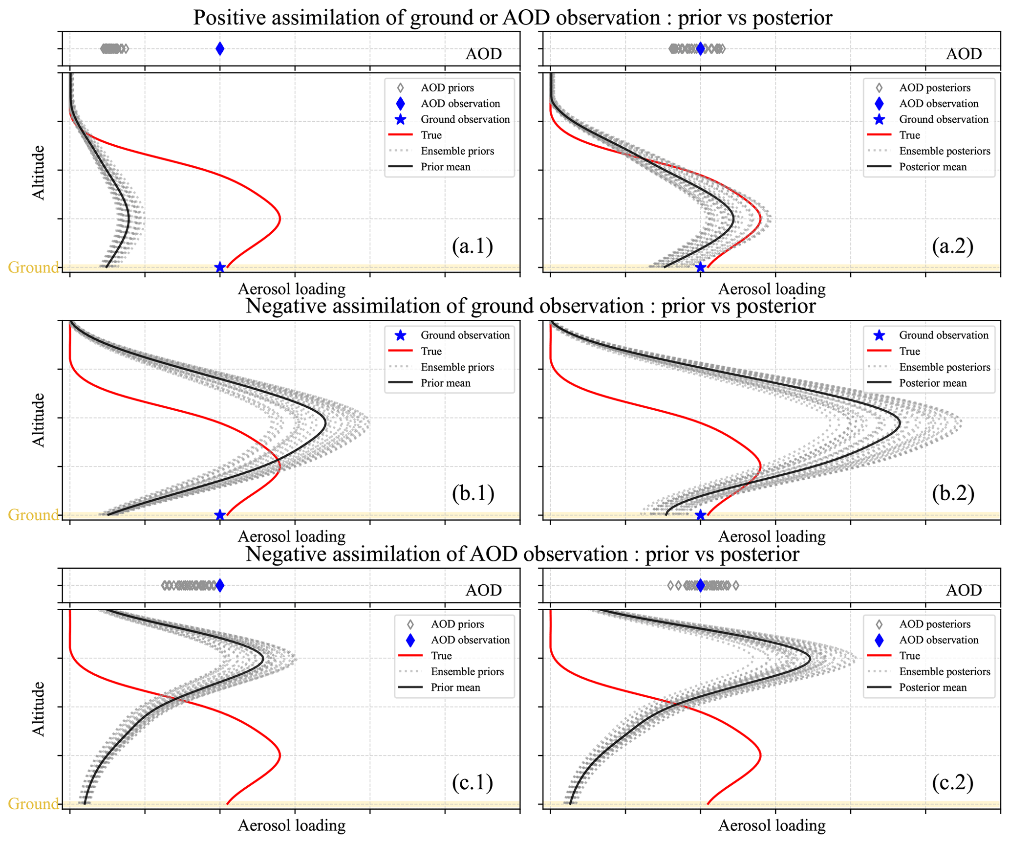
Figure 2 Schematic diagram of the sensitivity of data assimilation to aerosol vertical structure. Assimilation of ground and AOD observations under a positive condition, with AOD priors (hollow grey diamond) and AOD observations (solid blue diamond) in the upper box and true profiles (red line), ensemble priors (dashed grey line), prior means (black line), and ground observations (blue star) in the lower box (a.1). The figures on the right show the posteriors (a.2). The figures in the second row show the prior (b.1) and posterior (b.2) of the ground assimilation under a negative condition. The figures in the third row show the prior (c.1) and posterior (c.2) of the AOD assimilation under a negative condition.

3.2 Ground PM₁₀ assimilation

In this section, the impact of ground measurement data assimilation on the aerosol vertical structure is explained. In practice, each of the PM₁₀ observations could be assimilated to optimize the 3D states that are correlated. The increments are transferred from the observation space to the model space via the Kalman gain K shown previously. To easily evaluate the posterior, we solely perform the assimilation analysis at the pixels where PM₁₀ measurements are available. Thus, here we confine the states only in the vertical direction in one pixel to better identify the sensitivity, and we assume the prior states x^f with total k levels to be

$$\begin{array}{}\text{(9)}& {\displaystyle }{\displaystyle }{\mathit{x}}^f={\left[x_{\mathrm{1}}^f,\mathrm{\cdots }\mathrm{\cdots },x_k^f\right]}^{\mathrm{T}}.\end{array}$$

In this case, the error covariance matrix P^f is constructed by the variance of ensemble states and covariance in the vertical direction, and the observation operator 𝓗 only converts the single observation on the ground level:

$$\begin{array}{}\text{(10)}& {\displaystyle }& {\displaystyle }{\mathbf{P}}^f=\left[\begin{array}{cccc}{C}_{\mathrm{11}}& C_{\mathrm{12}}& \mathrm{\cdots }& C_{\mathrm{1}k}\\ C_{\mathrm{21}}& C_{\mathrm{22}}& \mathrm{\cdots }& C_{\mathrm{2}k}\\ \mathrm{⋮}& \mathrm{⋮}& \mathrm{\ddots }& \mathrm{⋮}\\ C_{k\mathrm{1}}& C_{k\mathrm{2}}& \mathrm{\cdots }& C_{kk}\end{array}\right],\text{(11)}& {\displaystyle }& {\displaystyle }\mathcal{H}=\left[\mathrm{1}\mathrm{0}\mathrm{\cdots }\mathrm{0}\right].\end{array}$$

The calculation of K follows Eq. (6) and substitutes Eq. (10) and Eq. (11) into it:

$$\begin{array}{ll}{\displaystyle }\mathbf{K}& {\displaystyle }={\mathbf{P}}^f{\mathcal{H}}^{\mathrm{T}}{\left(\mathcal{H}{\mathbf{P}}^f{\mathcal{H}}^{\mathrm{T}}+\mathbf{R}\right)}^{-\mathrm{1}}\\ \text{(12)}& {\displaystyle }& {\displaystyle }=[C_{\mathrm{11}},\mathrm{\cdots }\mathrm{\cdots },C_{k\mathrm{1}}{]}^{\mathrm{T}}(C_{\mathrm{11}}+{\mathit{\sigma }}_y^{\mathrm{2}}{)}^{-\mathrm{1}},\end{array}$$

where ${\mathit{\sigma }}_y^{\mathrm{2}}$ is the error in the ground observation.

We substitute K into the following update function:

$$\begin{array}{ll}{\displaystyle }& {\displaystyle }[x_{\mathrm{1}}^a,\mathrm{\cdots }\mathrm{\cdots },x_k^a{]}^{\mathrm{T}}={\left[x_{\mathrm{1}}^f,\mathrm{\cdots }\mathrm{\cdots },x_k^f\right]}^{\mathrm{T}}\\ \text{(13)}& {\displaystyle }& {\displaystyle }+[C_{\mathrm{11}},\mathrm{\cdots }\mathrm{\cdots },C_{k\mathrm{1}}{]}^{\mathrm{T}}(C_{\mathrm{11}}+{\mathit{\sigma }}_y^{\mathrm{2}}{)}^{-\mathrm{1}}(y-x_{\mathrm{1}}^f).\end{array}$$

Here, we have the posterior state $x_i^a$ on each level.

On the ground level, the posterior state is obtained as

$$\begin{array}{}\text{(14)}& {\displaystyle }{\displaystyle }{\mathit{x}}_{\mathrm{1}}^a={\displaystyle \frac{{\mathit{\sigma }}_y^{\mathrm{2}}}{C_{\mathrm{11}}+{\mathit{\sigma }}_y^{\mathrm{2}}}}{\mathit{x}}_{\mathrm{1}}^f+{\displaystyle \frac{C_{\mathrm{11}}}{C_{\mathrm{11}}+{\mathit{\sigma }}_y^{\mathrm{2}}}}y.\end{array}$$

If the observation error is much smaller than the prior error (${\mathit{\sigma }}_y^{\mathrm{2}}\ll C_{\mathrm{11}}$), we can have

$$\begin{array}{}\text{(15)}& {\displaystyle }{\displaystyle }{x}_{\mathrm{0}}^a\approx y,\end{array}$$

which means that the posterior on the ground level is close to that of the ground observation. The ground data assimilation has successfully tuned the ground prior state.

On the other hand, for the state on the ith level, the posterior $x_i^a$ is calculated by

$$\begin{array}{}\text{(16)}& {\displaystyle }{\displaystyle }{x}_i^a=x_i^f+{\displaystyle \frac{C_{k\mathrm{1}}}{C_{\mathrm{11}}+{\mathit{\sigma }}_y^{\mathrm{2}}}}(y-x_{\mathrm{1}}^f).\end{array}$$

To better identify the correctness of the vertical structure, we define a vertical ratio v_k here:

$$\begin{array}{}\text{(17)}& {\displaystyle }{\displaystyle }{v}_k={\displaystyle \frac{x_i}{x_{\mathrm{1}}}},\end{array}$$

which is the ratio of the state on the ith level to the ground level.

We divide $x_i^f$ on both sides of Eq. (16):

$$\begin{array}{}\text{(18)}& {\displaystyle }{\displaystyle }{v}_i^a=v_i^f+{\displaystyle \frac{C_{k\mathrm{1}}}{C_{\mathrm{11}}+{\mathit{\sigma }}_y^{\mathrm{2}}}}{\displaystyle \frac{y-x_{\mathrm{1}}^f}{x_{\mathrm{1}}^f}}.\end{array}$$

When we have a strong vertical correlation and small observation error, we have $\frac{C_{k\mathrm{1}}}{C_{\mathrm{11}}+{\mathit{\sigma }}_y^{\mathrm{2}}}\approx \mathrm{1}$. If the prior vertical structure is far from the true structure, $v_i^f\ll v_i^{\text{true}}$ or $v_i^f\gg v_i^{\text{true}}$. Then, the vertical structure of the posterior is strongly dependent on $\frac{y-x_{\mathrm{1}}^f}{x_{\mathrm{1}}^f}$. If $x_{\mathrm{1}}^f$ and y deviate far from each other, the increment can be large, thus further enhancing the incorrect prior structure $v_i^f$.

Figure 2b illustrates this kind of pattern. In panel (b.1), the priors greatly underestimate the aerosol concentration on the ground level. Meanwhile, over the upper space, the priors overestimate the intensity and altitude of the dust loading to some extent. After assimilating the ground observations, as shown in panel (b.2), the posterior aerosol loading (dashed grey line) is tuned to a large extent and is much closer to the observation on the ground layer, while for the vertical distribution, a greater overestimation than that of the prior can be seen. The original incorrect profile is significantly amplified.

3.3 AOD assimilation

Assimilation of AOD-related observations is carried out by connecting the 3D aerosol priors x^f and AOD priors τ^f. It is assumed that the vertical structure of the aerosol field remains the same as the AOD lacks vertical information. Then, a 3D mass concentration field can be calculated by finding the optimal AOD field.

To begin with, the value of the AOD is related to the aerosol mass concentration, aerosol type, and humidity. Here, it is assumed to be linearly related to only the aerosol mass concentration field x^f. The column-integrated AOD is calculated by summing the aerosol mass concentration ${\mathit{x}}_i^f$ on each level:

$$\begin{array}{}\text{(19)}& {\displaystyle }{\displaystyle }{\mathit{\tau }}^f=\sum _{i=\mathrm{1}}^k\mathcal{M}{\mathit{x}}_i^f,\end{array}$$

where ℳ is the linear model operator that calculates the AOD from the mass concentration.

The calculation of the posterior AOD, τ^a, follows Eq. (8):

$$\begin{array}{}\text{(20)}& {\displaystyle }{\displaystyle }{\mathit{\tau }}^a={\stackrel{\mathrm{‾}}{\mathit{\tau }}}^f+\mathbf{K}(\mathit{y}-\mathcal{H}{\stackrel{\mathrm{‾}}{\mathit{\tau }}}^f).\end{array}$$

Next, we substitute Eq. (19) into Eq. (20). We can then bridge the mass concentration field and AOD field:

$$\begin{array}{}\text{(21)}& {\displaystyle }{\displaystyle }\mathcal{M}\sum _{i=\mathrm{1}}^k{\mathit{x}}_i^a=\mathcal{M}\sum _{i=\mathrm{1}}^k{\stackrel{\mathrm{‾}}{\mathit{x}}}_i^f+\mathbf{K}(\mathit{y}-\mathcal{H}{\stackrel{\mathrm{‾}}{\mathit{\tau }}}^f).\end{array}$$

Similarly for AOD, we confine the states in the vertical direction within one pixel. We have one prior AOD, τ^f, and aerosol mass prior, $x_i^f$, on a total of k levels. We first define a vertical factor, u_i, which is the ratio of the mass at the ith level to the mass at all levels:

$$\begin{array}{}\text{(22)}& {\displaystyle }{\displaystyle }{u}_i={\displaystyle \frac{x_i}{\sum _{i=\mathrm{1}}^k{x}_i}}.\end{array}$$

Next, we substitute it into Eq. (21):

$$\begin{array}{}\text{(23)}& {\displaystyle }{\displaystyle }\mathcal{M}{\displaystyle \frac{x_i^a}{u_i}}=\mathcal{M}{\displaystyle \frac{x_i^f}{u_i}}+\mathbf{K}(y-\mathcal{H}{\mathit{\tau }}^f).\end{array}$$

Since we have only one observation and one AOD simulation, the observation operator 𝓗, error variance matrix P^f, and Kalman gain K are

$$\begin{array}{}\text{(24)}& {\displaystyle }{\displaystyle }\mathcal{H}=\left[\mathrm{1}\right],{\mathbf{P}}^f=\left[{\mathit{\sigma }}_{\mathit{\tau }}^{\mathrm{2}}\right],\mathbf{K}=\left[{\displaystyle \frac{{\mathit{\sigma }}_{\mathit{\tau }}^{\mathrm{2}}}{{\mathit{\sigma }}_{\mathit{\tau }}^{\mathrm{2}}+{\mathit{\sigma }}_y^{\mathrm{2}}}}\right].\end{array}$$

We substitute them into Eq. (23), which gives us the mass posterior $x_i^a$ on each layer:

$$\begin{array}{}\text{(25)}& {\displaystyle }& {\displaystyle }\mathcal{M}{\displaystyle \frac{x_i^a}{u_i^f}}=\mathcal{M}{\displaystyle \frac{x_i^f}{u_i^f}}+{\displaystyle \frac{{\mathit{\sigma }}_{\mathit{\tau }}^{\mathrm{2}}}{{\mathit{\sigma }}_{\mathit{\tau }}^{\mathrm{2}}+{\mathit{\sigma }}_y^{\mathrm{2}}}}(y-{\mathit{\tau }}^f),\text{(26)}& {\displaystyle }& {\displaystyle }{x}_i^a=x_i^a+u_i^f{\displaystyle \frac{{\mathit{\sigma }}_{\mathit{\tau }}^{\mathrm{2}}}{{\mathit{\sigma }}_{\mathit{\tau }}^{\mathrm{2}}+{\mathit{\sigma }}_y^{\mathrm{2}}}}{\displaystyle \frac{y-{\mathit{\tau }}^f}{\mathcal{M}}}.\end{array}$$

This equation demonstrates that the analysis increment $\frac{{\mathit{\sigma }}_{\mathit{\tau }}^{\mathrm{2}}}{{\mathit{\sigma }}_{\mathit{\tau }}^{\mathrm{2}}+{\mathit{\sigma }}_y^{\mathrm{2}}}\frac{y-{\mathit{\tau }}^f}{\mathcal{M}}$ from AOD assimilation is allocated to each level of mass by the vertical factor u_i. When we have an incorrect structure, we note that $u_i\gg u_i^{\text{true}}$ or $u_i\ll u_i^{\text{true}}$. The analysis increment can be reallocated to the wrong level, thus amplifying the incorrect structure.

Figure 2c demonstrates the negative pattern of assimilating AOD. In the upper row of panel (c.1), we have the ensemble AOD priors (hollow grey diamond) and the AOD observation (solid blue diamond) that are combined to optimize the 3D dust mass field (dashed grey line). Similar to panel (b), assume we have an incorrect prior dust mass structure. By assimilating AOD observations, the AOD posteriors can be tuned to better fit the AOD observation, as shown in the upper row in panel (c.2), while for the structure of mass field, this incorrect structure is generally amplified since the prior DOD simulation implies that the model underestimates the total dust column compared to the observation. Another pattern, in which the prior mass is incorrectly situated at the ground level, is also illustrated in Fig. S1 in the Supplement. It is notable that the sensitivity of AOD assimilation to the vertical structure is not as significant as that of the ground assimilation since the AOD contains information on the total columns.

3.4 Case settings

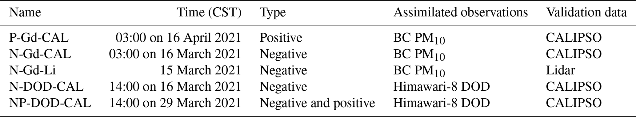
To demonstrate the sensitivity of aerosol data assimilation to vertical structure, five assimilation analysis cases were selected, namely P-Gd-CAL, N-Gd-CAL, N-Gd-Li, N-DOD-CAL, and NP-DOD-CAL. These cases were selected from the ensemble model run starting from 00:00 CST on 14 March to 00:00 CST on 17 March and 00:00 CST on 14 April to 00:00 CST on 17 April 2021. (Hereafter, all times are in CST.) Dust classification is carried out using the CALIPSO depolarization ratio data to ensure that dust is the dominant particle during these time ranges. The procedures and results can be found in the Supplement. The background run consists of 32 ensembles, and each of them are driven by perturbed emission inventories. Details concerning the generation of the ensembles can be found in Jin et al. (2022).

Figure 1 lists information about the experiment cases. P-Gd-CAL is a positive case, which shows how the data assimilation corrects the surface concentrations and maintains the correct aerosol structure. N-Gd-CAL and N-Gd-Li are negative cases, which show how the assimilation deteriorates the profile when assimilating ground observations only. The time of the former two cases is fixed, and their profiles follow the trajectory of CALIPSO. Hence, by comparison, we can observe the impact of assimilation on the vertical structure. The last case focuses on a fixed site. A continuous timeline is used, and assimilation analysis is performed on each time point. The profiles are compared with high-resolution lidar observations. N-DOD-CAL and NP-DOD-CAL are negative cases that focus on assimilating DOD observations. Himawari-8 DOD observations are assimilated. Both of them are validated by CALIPSO.

In addition, to test the impact of vertical localization on the assimilation performance, experiments applying EnKF with vertical localization are also carried out. They are performed on the priors of cases P-Gd-CAL and P-Gd-CAL. These results can be found in the Supplement.

Table 1 Experiment configurations.

4 Results and discussions

This section delves into the sensitivities of data assimilation from ground and DOD observations, with a particular emphasis on the impact of prior vertical profiles. Regarding the ground observation assimilation, the discussion is enriched by presenting a positive case, alongside two illustrative negative examples. The validity of these scenarios is further reinforced by CALIPSO satellite observations and lidar measurements. This serves to underscore the substantial influence that ground assimilation can exert on the posterior. Then, the examination of DOD assimilation uncovers its intricacies by showcasing two instances, highlighting favourable and unfavourable outcomes. These illustrations collectively emphasize the impact DOD assimilation has on the posterior, thereby underscoring the importance of understanding the vertical profile's role in the assimilation process for both ground and DOD observations.

4.1 Cases on ground assimilation

4.1.1 Positive case

P-Gd-CAL is intended to demonstrate how the assimilation works properly. Figure 3a.1 shows the time series of ground PM₁₀ and BC PM₁₀ from several ground stations that are close to the CALIPSO trajectory (<0.25°). The assimilation time point, 03:00 on 16 April 2021, is selected in this case (highlighted in green). Although it is during the later stage of the dust storm, the concentrations were as high as approximately 400 µg m⁻³. Through comparison between raw and bias-corrected PM₁₀ (solid and dashed lines), it is clear that the scanned region was still dominated by coarse-dust aerosol. Figure 3c.1 and d.1 are snapshots of the average of ensemble priors and posteriors. We can see that the priors underestimated the dust load to the south of the domain and overestimated it to the east. After assimilation analysis, the dust load was adjusted to better fit the observations. The ground observations were consistent with the posterior. RMSE was reduced from 254.83 to 118.03 µg m⁻³.

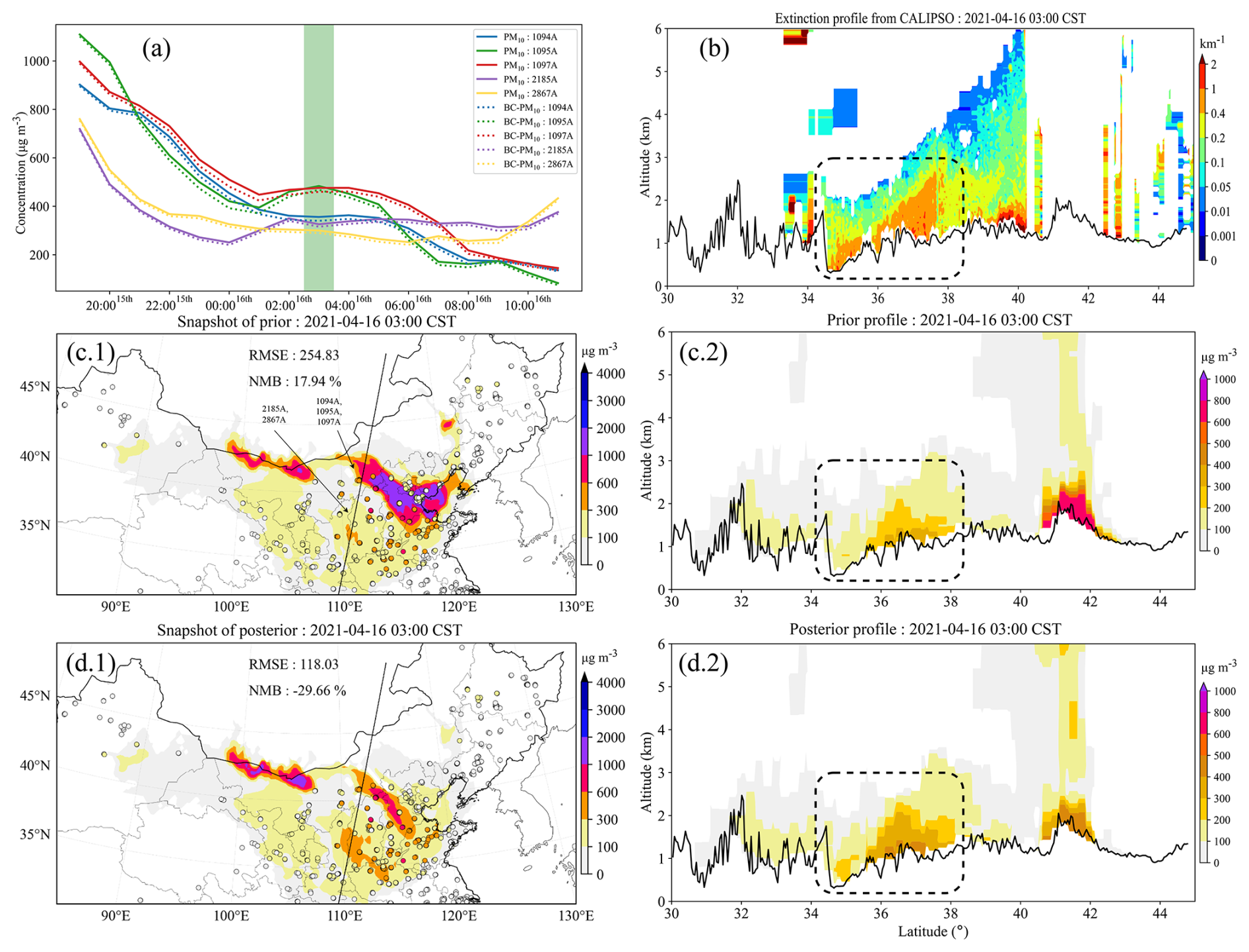
Figure 3 Time series of PM₁₀ and BC PM₁₀ concentrations from several ground stations that are close to the CALIPSO trajectory (a). Spatial distribution of ground dust concentrations from the average of the ensemble priors and the posteriors with scatters of ground BC PM₁₀ observations (c.1 and posterior d.1). The black line inside is where CALIPSO scanned through. The figures in the right column are the extinction profile from CALIPSO (b) and the dust concentration profile following the CALIPSO scanning trajectory from the prior (c.2) and the posterior (d.2). The colour bars in (c.2) and (d.3) are rescaled to show more detail. The black line at the bottom is the terrain altitude. The case time is at 03:00 CST on 16 April 2021.

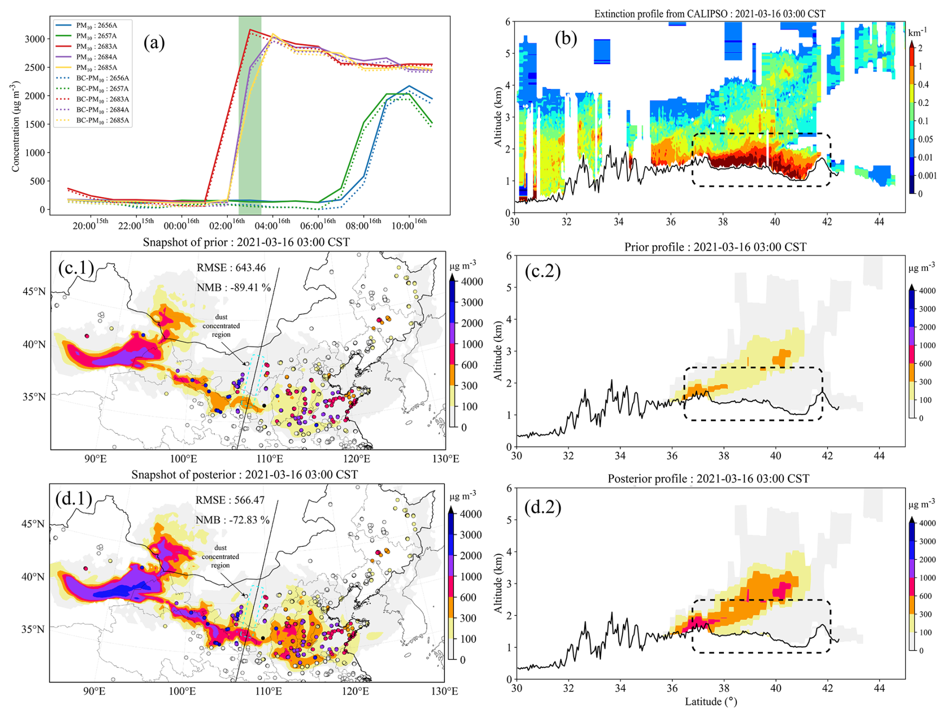
Figure 4 Time series of PM₁₀ and BC PM₁₀ concentrations from several ground stations that are close to the CALIPSO trajectory (a). Spatial distribution of ground dust concentrations from the average of the ensemble priors and the posteriors with scatters of ground BC PM₁₀ observations (c.1 and posterior d.1). The black line inside is where the CALIPSO scanned through. The figures in the right column are the extinction profile from CALIPSO (b) and the dust concentration profile following the CALIPSO scanning trajectory from the prior (c.2) and the posterior (d.2). The black line at the bottom is the terrain altitude. The case time is at 03:00 CST on 16 March 2021.

Take a closer look at the vertical structure. Figure 3b illustrates the extinction coefficient profile from CALIPSO. From the profile we can tell that the dust was concentrated on the ground over a latitude of 34–38° (circled by the dashed line). Vertically, it extended upwards, accompanied with terrain from 1 km at 34.5° to 2.5 km at 37.5°. Figure 3c.1 shows the prior dust profile following the same trajectory of CALIPSO. The colour bar here is rescaled to show more detail. At around 41–42°, a heavy dust load was simulated (600–800 µg m⁻³), while CALIPSO did not capture the data there. Hence, it cannot be validated, and we focus on the dust at 34–38°. At 34–38°, the prior model had successfully reproduced the dust structure indicated by CALIPSO. The concentrations were about 100–300 µg m⁻³, which are underestimated, as shown in Fig. 3d.2. After assimilation, the ground concentrations increased to 400–500 µg m⁻³, as shown in (c.1) and (d.1). The vertical structure was also reserved, which is identical to the structure shown by CALIPSO.

4.1.2 Negative case validated by CALIPSO

N-Gd-CAL is the negative case that illustrates how data assimilation degrades the aerosol vertical structure. Figure 4a.1 shows the time series of ground PM₁₀ and BC PM₁₀ from several ground stations that are close to the CALIPSO trajectory. As shown in panel (a), the ground dust aerosol loading from ground stations in N-Gd-CAL increased rapidly starting 2 h before assimilation occurred. This means that the region in the lower rectangle in (c.1) was a dust-concentrated region.

Evidence from CALIPSO also indicated that there was heavy dust loading. As shown in Fig. 4b, the extinction coefficient profile from 37 to 42° (circled by the dashed black rectangle) exhibits extremely high values (maximum exceeded 2 km⁻¹). It spread upwards for 1 km at an altitude of 1 km. This region is highlighted by the dashed light blue rectangle in (c.1) and (d.1). As inferred from the farther ground stations (concentrations over 1000 µg m⁻³), this region was dominated by dust aerosols and is situated at ground level.

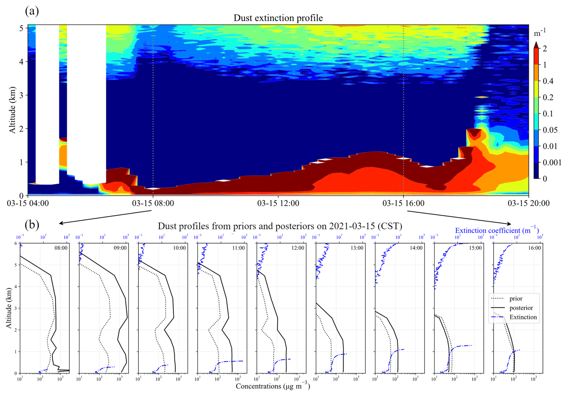
Figure 5 Time series of dust extinction coefficient profile obtained from lidar (a). The assimilation analysis is performed hourly from 08:00 to 16:00. The figure below shows the hourly dust profile line from priors (dashed line) and posteriors (solid line) (b). The extinction coefficient is also plotted (dash-dotted blue line). The profile data are extracted from the closest grid point to the lidar location. The x axis is logarithmically rescaled. Note that instead of using the posterior in the previous time step to propagate the model, analysis here is separately conducted on the static background.

The dust profile in (c.2) indicates that the ensemble priors agreed that the aerosols were mainly concentrated upwards. The plume floated up to 4 km with latitude. Only a few dust aerosols over 36–37° on the ground (300–600 µg m⁻³) show consistency with the observations (shown in c.1 and c.2). A great discrepancy exists between the prior and independent observations at 37–42°. After assimilating BC PM₁₀ concentrations, the overall loading is increased. The great underestimation in the east is improved. However, the dust-concentrated region circled in (d.1) is only improved to a small extent. This is due to a lack of observations nearby and the much lower uncertainties exhibited by ensemble priors. In terms of the vertical structure, a disturbing profile is obtained. As shown in Fig. 4d.2, ground concentrations at 36–37° are aligned to over 600 µg m⁻³. This is consistent with surrounding stations. However, for the reason mentioned earlier, dust loads over 37–42° are barely corrected. Yet, these trivial increments significantly enhance the erroneous vertical structure. At ground level, the dust concentrations rise from less than 100 µg m⁻³ to nearly 300 µg m⁻³ at 37–39°. The vertical loading is almost 3 times greater than the loading from the prior profile. Moreover, the extremely low region at 39–42° represents a more intense amplification effect than that. Since the low values are more sensitive to variations, increments on these values can easily give rise to an increase in the vertical loading. In this case, this phenomenon can be seen clearly through the comparison between priors, posteriors, and measurements for validation.

4.1.3 Negative case validated by lidar

N-Gd-Li is another negative case. In this case, we do not focus on a single time point. A series of assimilation analyses is conducted to investigate the effect. As shown by Fig. 5a, a high-resolution profile of a dust extinction coefficient from lidar is given to demonstrate the changing structure of dust loading on a fixed location. Entering at about 05:00 and then landing at 07:00, this dust storm lasted for about 20 h in the area where the lidar was located. A time range from 08:00 to 16:00 is selected as it comprises most of the dust period. During the whole period, the measured dust loading increased from 0.4 to 1.4 km. Afterwards, the intensity decreased gradually.

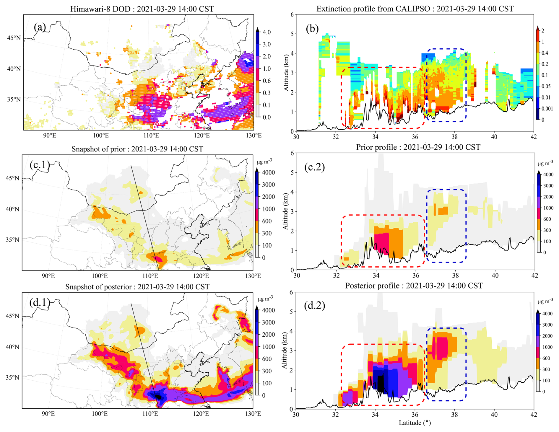
Figure 6 Time series of PM₁₀ and BC PM₁₀ concentrations from several ground stations that are close to the CALIPSO trajectory (a). Spatial distribution of ground dust concentrations from the average of the ensemble priors and posteriors with scatters of ground BC PM₁₀ observations (c.1 and posterior d.1). The black line inside is where CALIPSO scanned through. The figures in the right column are the extinction profile from CALIPSO (b) and dust concentration profile following the CALIPSO scanning trajectory from the prior (c.2) and the posterior (d.2). The black line at the bottom is the terrain altitude. The case time is at 14:00 CST on 29 March 2021.

Figure 5b illustrates the hourly prior and posterior dust profiles during the selected period. The profiles of the extinction coefficient are also plotted with the dash-dotted blue line. The x axis, which represents concentrations, is logarithmically rescaled here. In terms of prior profiles, dust loading extended up to 5 km at 08:00 and declined to 3 km at 16:00. This structure is inconsistent with the lidar profile, in which only little dust was observed. The dust storm has been overestimated to a large extent in height. The ground aerosol concentrations are lower than 200 µg m⁻³ throughout eight time points, which is much lower than those of the observations (over 1000 µg m⁻³). After assimilation, this underestimation is mitigated. The ground dust concentrations are amplified several times to better fit the observations. Meanwhile, the erroneous vertical structure is also intensified in the first six moments, as can clearly be seen in the comparison between the concentration and extinction coefficient. At 09:00 in particular, the dust loading above 2 km is amplified to over 1000 µg m⁻³, which will provide completely incorrect information about the dust storm structure and impact future forecasting.

4.2 Cases on DOD assimilation

In this section, the sensitivity of assimilating DOD to the aerosol vertical profile is presented, starting with the NP-DOD-CAL case. Figure 6a shows the spatial distribution of DOD observed by Himawari-8 at 14:00 on 29 March 2021. The dust plume approached the east of China and reached out to the East China Sea. The prior model reproduces the distribution, while the overall concentration is underestimated (less than 300 µg m⁻³), as shown in panel (c.1). By assimilating the Himawari-8 DOD, the overall dust concentration field is increased to over 1000 µg m⁻³. The posterior dust plume is consistent with the DOD observations.

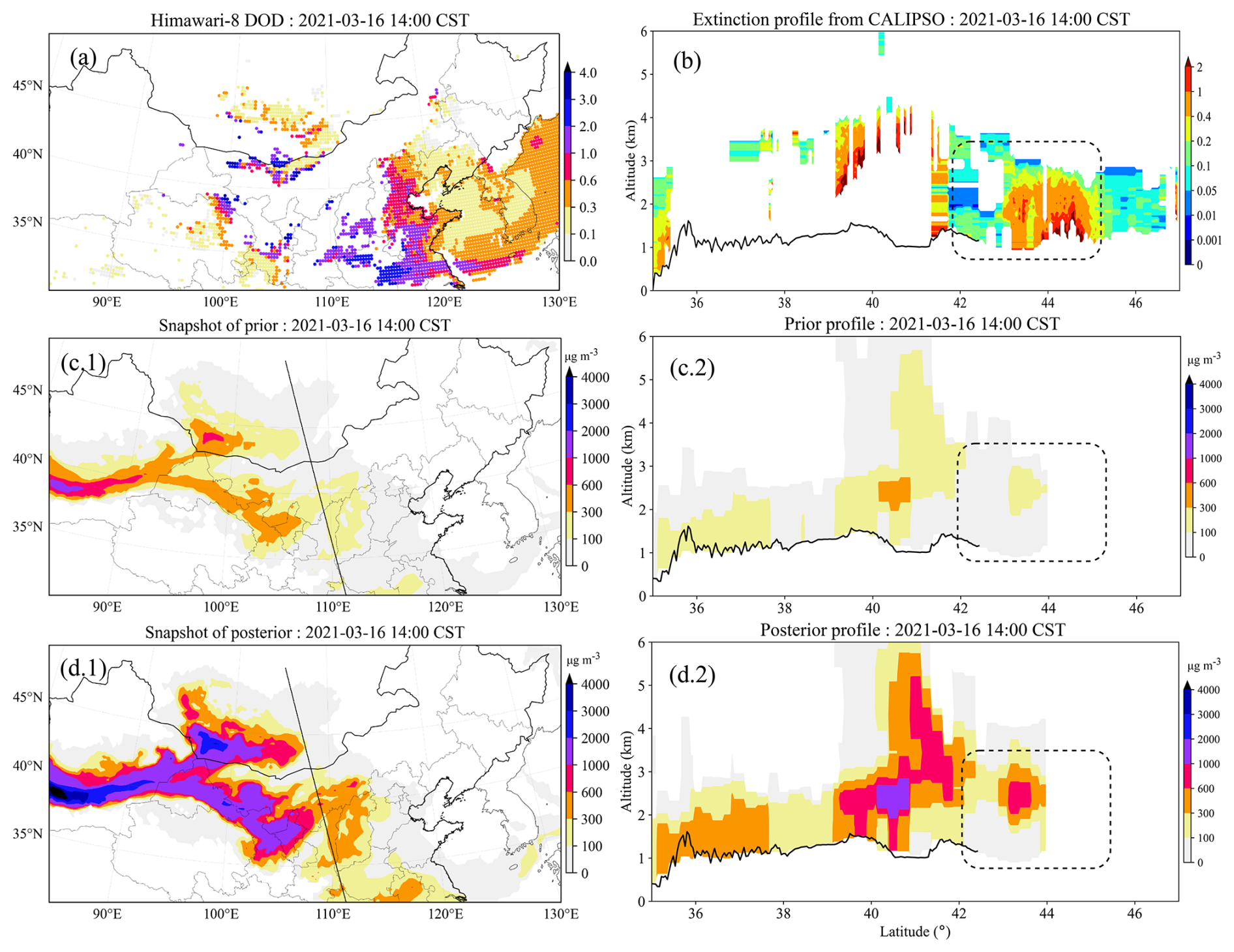
Figure 7 Snapshot of Himawari-8 DOD at the assimilation instance (a). Spatial distribution of ground dust concentrations from the average of the ensemble priors (c.1 and posterior d.1). The black line inside is where CALIPSO scanned through. The figures in the right column are the extinction profile from CALIPSO (b) and the dust concentration profile following the CALIPSO scanning trajectory from the prior (c.2) and the posterior (d.2). The black line at the bottom is the terrain altitude. The case time is at 14:00 CST on 16 March 2021.

As shown by the extinction profile in panel (b), the dust was concentrated around 32–38° and extended upwards to an altitude of 3 km. In terms of the prior, this structure is partly correct. The dust in the red box is located on the lower layer and aligns with the extinction profile, while the dust in the blue box has a higher position. By assimilating DOD, the total column dust field is optimized, and the vertical structure is restored following the prior dust field. As a result, the underestimation is alleviated, and the overall concentrations are increased. The correct dust structure in the red box is maintained, and the intensity is enhanced. However, the incorrect dust structure in the blue box is also amplified, causing an obvious inaccurate dust loading, which should be located on the lower level.

N-DOD-CAL is another case that illustrates the negative aspects of assimilating DOD. Figure 7 comprises the same assimilation experiment results as in NP-DOD-CAL, except at 14:00 on 16 March 2021. The DOD observations report high values densely distributed in the east and sparsely distributed in the north. The prior model simulates the dust plume that is concentrated in the north-west. To the east, only rare dust is observed. It is caused by the inability of the model to reproduce the long-term transport of dust. If we focus on where CALIPSO scanned through, an increase in dust can be seen.

In terms of CALIPSO, it is certain that the dust is concentrated on the lower level at 43–45°. There is also a dust plume at 39–42°, although it cannot be verified because of the missing observation data. Similarly, the prior dust profiles show an incorrect dust structure, as circled by the black box in panel (c.2). After assimilation, this error is amplified from around 100 µg m⁻³ to over 600 µg m⁻³.

5 Conclusions

Data assimilation has been widely used in constructing reanalysis datasets and improving the predictability of atmospheric models. The performance of assimilation algorithms relies not only on the methodologies themselves but also on the observations. Nowadays, the complexity and dimensions of atmospheric models have been growing rapidly. For atmospheric aerosol models, high spatial and temporal resolutions are becoming feasible. In terms of observations, they are either outnumbered in space or discontinuous in time compared to models. Particularly in the vertical direction, the available aerosol measurements are still limited both in space and in time. Through assimilating ground or satellite measurements, the aerosol field can be improved, while in 3D space, it can also amplify the erroneous estimation of the aerosol structure.

In this paper, we explore the sensitivity of aerosol data assimilation to the vertical profile by carrying out five assimilation experiments. Dust aerosol, which is simulated by LOTOS-EUROS, is selected as the optimization target. The EnKF data assimilation methodology is adopted. Bias-corrected ground PM₁₀ concentrations obtained from ground monitoring stations and DOD from Himawari-8 are assimilated. An extinction coefficient profile from CALIPSO and polarization lidar are used to validate the aerosol vertical structure. P-Gd-CAL intends to show how ground data assimilation tunes the vertical structure positively. After assimilation, the ground dust field is optimized to better fit the observations, and the vertical structure is enhanced, which is also consistent with the CALIPSO measurements. In contrast, N-Gd-CAL exhibits a drastic negative effect. In this case, even small increments on the ground can greatly enhance the incorrect aerosol structure. N-Gd-Li is another negative case that displays hourly prior and posterior profiles. The continuous dust extinction profile from lidar is utilized to validate the structure. In most of the moments, the assimilation improves the ground aerosol field while significantly degrading the vertical dust loading. N-DOD-CAL and NP-DOD-CAL intend to show how DOD assimilation deteriorates the vertical structure. Different from the ground assimilation, the posterior vertical structure is here reallocated by the vertical ratio. When the vertical ratio is incorrect, assimilating DOD can also pass down this error.

In conclusion, integrating ground- and satellite-derived aerosol observations into models enhances both the analysis and the forecasting accuracy of the model's state. However, challenges persist in reconciling these observations with the model's high-dimensional state. Specifically, the model's initial, potentially flawed vertical aerosol structure could impair assimilation efforts. The underlying reason is that data assimilation relies on the background error covariance to propagate the innovations between states and observations across the entire domain. If the vertical structure is inaccurate, this error may not only persist but could also be amplified during the assimilation process. Analytical examples from both ground-based and satellite-based assimilation confirm this effect. This paper has only scratched the surface by presenting a handful of negative instances, yet it is evident that this issue is pervasive in aerosol data assimilation. The path forward entails establishing a complementary network of vertical observations and implementing advanced assimilation methodologies that are sensitive to vertical structures, thereby offering a promising avenue to surmount these challenges.

Appendix A: Conversion of AOD between different wavelengths

One common method for converting AOD between different wavelengths involves the Ångström exponent ($\stackrel{\mathrm{˚}}{A}$) (Jin et al., 2023b). This exponent describes the relationship between AOD and wavelength, defined as the ratio of the logarithm of the AOD ratio at two different wavelengths to the logarithm of the ratio of those wavelengths:

$$\begin{array}{}\text{(A1)}& {\displaystyle }{\displaystyle }\stackrel{\mathrm{˚}}{A}=-{\displaystyle \frac{\log ({\mathit{\tau }}_{{\mathit{\lambda }}_{\mathrm{1}}}/{\mathit{\tau }}_{{\mathit{\lambda }}_{\mathrm{2}}})}{\log ({\mathit{\lambda }}_{\mathrm{1}}/{\mathit{\lambda }}_{\mathrm{2}})}},\end{array}$$

where $\stackrel{\mathrm{˚}}{A}$ is the Ångström exponent. ${\mathit{\tau }}_{{\mathit{\lambda }}_{\mathrm{1}}}$ and ${\mathit{\tau }}_{{\mathit{\lambda }}_{\mathrm{2}}}$ are the AOD values at wavelengths λ₁ and λ₂, respectively.

Given the AOD at a specific wavelength and the Ångström exponent, the AOD at another wavelength can be estimated using the following formula:

$$\begin{array}{}\text{(A2)}& {\displaystyle }{\displaystyle }{\mathit{\tau }}_{\mathit{\lambda }}={\mathit{\tau }}_{{\mathit{\lambda }}_{\mathrm{0}}}{\left({\displaystyle \frac{\mathit{\lambda }}{{\mathit{\lambda }}_{\mathrm{0}}}}\right)}^{-\stackrel{\mathrm{˚}}{A}}.\end{array}$$

Here, λ₀ represents the reference wavelength where the AOD is known, and λ is the target wavelength. The wavelengths 550 and 532 nm are very close in the visible spectrum, with a difference of only 18 nm. Dust optical properties, such as extinction coefficient, do not vary significantly over such a small wavelength range. This allows for a reasonable approximation when comparing data at these two wavelengths.

Appendix B: DOD operator

Mie theory is applied to convert the aerosol mass concentration into AOD. It is calculated through the scatter and absorption coefficients of spherical particles with a given radius and refractive index (Gupta et al., 2018) and is defined as

$$\begin{array}{}\text{(B1)}& {\displaystyle }{\displaystyle }\mathit{\tau }=\sum _{k=\mathrm{1}}^n{\mathit{ϵ}}_{\mathrm{d}}^k{z}^k,\end{array}$$

where τ is the simulated AOD. ${\mathit{ϵ}}_{\mathrm{d}}^k$ and z^k are the dust extinction coefficient and layer thickness at the kth layer. ${\mathit{ϵ}}_{\mathrm{d}}^k$ is calculated by the product of extinction efficiency Q_ext, the total cross section per unit mass S (m² g⁻¹), and the aerosol mass concentration C (g m⁻³):

$$\begin{array}{}\text{(B2)}& {\displaystyle }{\displaystyle }{\mathit{ϵ}}_{\mathrm{d}}^k=Q_{\text{ext}}SC,\end{array}$$

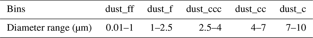
where Q_ext is the sum of the scattering and absorption efficiency. It is decided by the ratio of the aerosol radius, the incident wavelength, and the chemical composition (van de Hulst, 1958). S depends on the particle size and aerosol mass density. The dust bins and diameter ranges are shown in Table B1. Detailed descriptions concerning the calculation of Q_ext and S can be found in Sect. 2 in Jin et al. (2023b).

Table B1 Dust size bins and diameter ranges.