Wastewater matters: incorporating wastewater treatment and reuse into a process-based hydrological model (CWatM v1.08)

Wastewater treatment and reuse are becoming increasingly critical for enhancing water use efficiency and ensuring reliable water availability. Wastewater also significantly influences hydrological dynamics within urban watersheds. Although hydrological modeling has advanced to incorporate human–water interactions, large-scale and multi-resolution models often lack the comprehensive integration of wastewater treatment and reuse processes. This paper presents the new wastewater treatment and reuse module as part of the hydrological Community Water Model (CWatM) and demonstrates its capabilities and advantages in an urban watershed with intermittent flows. Incorporating wastewater into the model improves model performance by better representing low and peak flows during the respective dry and wet seasons. It allows for the representation of sectoral wastewater reuse, the exploration of different measures to increase wastewater reuse, and the examination of the effects of wastewater reuse on the water stress level. Modeling wastewater treatment and reuse is particularly relevant in regions with semi-arid or arid climates, rapid urbanization, or active policies promoting water reuse. The wastewater treatment and reuse module could be upscaled by minimizing the data requirements via simplified workflows. Combined with the availability of recent datasets on wastewater treatment plants and processes, a global application of the module is feasible. As current developments focus on water quantity, the water quality dimension of wastewater treatment remains a limitation. This opens prospects for incorporating water quality into the model and developing global input data for wastewater treatment and reuse.

1 Introduction

Over the last few decades, hydrological modeling has developed to account for the human–water interface (Wada et al., 2017). Recent developments in this field have focused on developing higher-resolution global hydrological models (GHMs) by increasing models' spatial resolution, adjusting their datasets, and including a variety of water management options (Abeshu et al., 2023; Hoch et al., 2023; Burek et al., 2020; Hanasaki et al., 2022).

Increasing human interventions in the water cycle and higher-spatial-resolution modeling have emphasized the need to include water management as an integral part of hydrological models (Hanasaki et al., 2022). Some large-scale hydrological models (LHMs) already account for water management aspects, like water withdrawal and consumption, irrigation management, reservoir operations, water transfers, and desalination (Wada et al., 2017).

Wastewater treatment and reuse are other management options that are increasingly important in many regions. Currently, treated wastewater is estimated to be 188 km³ yr⁻¹ globally, which is around 52 % of the effluents generated. Further, approximately 22 % (of treated wastewater) is estimated to be reused (Jones et al., 2021). Thebo et al. (2017) found that around 35.9×10⁶ ha of irrigated cropland is supported by rivers dominated by wastewater from upstream urban areas, and Van Vliet et al. (2021) indicated that expansion of treated wastewater use from 1.6×10⁹ to 4.0×10⁹ m³ per month could strongly reduce water scarcity levels worldwide.

Specifically, wastewater reuse is a valuable water source for industrial and irrigation applications in water-stressed regions. For example, Israel reuses around 88 % of its treated wastewater, mainly for use in the agricultural sector, where it satisfies about 45 % of the agricultural water withdrawals (Fridman et al., 2021). Treated wastewater is also used for irrigation in southern European, Mediterranean, and North African countries (Angelakis et al., 1999; Bixio et al., 2006). While accepting exacerbated stress on freshwater resources, the European Parliament is working to improve the quality of wastewater treatment in the European Union, aiming to increase wastewater reuse (European Parliament, 2024). It follows that prospects of increased utilization of this resource are plausible.

Wastewater collection, treatment, and reuse are relevant processes for the hydrological modeling of urban catchments and complex water resource systems, and these processes are included in different small-scale models (Salvadore et al., 2015). Large-scale hydrological models often neglect wastewater treatment and reuse. However, to some extent, few models include wastewater treatment effects on water quality. The Soil and Water Assessment Tool (SWAT) includes septic tanks as an on-site treatment option. It simulates the percolation of wastewater into soils, the interaction between pollutants and the soil media, and bacteria buildup and nutrient uptake (Neitsch et al., 2011).

Another example is DynQual, a global water quality model coupled with the PCR-GLOBWB2 hydrological model (Jones et al., 2023). The model includes wastewater treatment processes in water quality simulations while also simplifying wastewater treatment and reuse management. Namely, in DynQual, wastewater is generated, collected, treated, and discharged locally (in a single grid cell).

While these are significant developments, they only partially capture the complex dynamics between human activities and hydrological processes occurring in urbanized catchments or otherwise complex water resource systems.

This paper introduces a recently developed, customizable wastewater treatment and reuse module as part of the Community Water Model (CWatM), allowing various modes of simulating wastewater treatment and reuse processes.

CWatM is a versatile, fully distributed, modular, and open-source hydrological model that simulates natural and anthropogenically affected hydrological processes at a daily time step and multiple spatial resolutions ranging from 0.5° to 30 arcsec (Burek et al., 2020). CWatM has extensive and publicly available documentation of the source code, the model structure, and model training and tutorials (https://cwatm.iiasa.ac.at/, last access: last access: 11 July 2024). The development of the wastewater treatment and reuse fits with the modularity and flexibility of CWatM by providing various modus operandi to enable the simulation of wastewater treatment and reuse on global (0.5°), regional (5 arcmin), and local (up to 30 arcsec) scales. This paper aims to introduce this module using a high-resolution (around 1 km²) case study of an urbanized river basin in a relatively dry climate (the Ayalon Basin in Israel).

The rest of the article is organized as follows: Sect. 2 describes the model development; Sect. 3 covers the case study, input data, and scenarios; and Sect. 4 presents the results, followed by discussion and conclusions in Sects. 5 and 6, respectively.

2 Module development and description

2.1 The Community Water Model (CWatM)

CWatM is a large-scale, distributed hydrological model suitable for implementation at global and regional scales (Burek et al., 2020). It is implemented in the Python programming language and is a fully open-source model (https://cwatm.iiasa.ac.at, last access: 11 July 2024). CWatM simulates the main hydrological processes and covers some aspects of the human–water interface. This paper presents the recently developed wastewater treatment module to enhance CWatM's capacity to address human water management. The model is applied to the relatively water-scarce Ayalon Basin in Israel. It uses a spatial resolution of 30 arcsec (∼1 km² grid) in a geographic coordinate system (WGS84). Groundwater is simulated by the coupled CWatM–MODFLOW6 model (Guillaumot et al., 2022) at a spatial resolution of 500 m using the UTM36N coordinate system.

2.2 Developing the wastewater treatment and reuse module (WTRM)

The wastewater treatment and reuse module (WTRM) enhances the capacity of CWatM to simulate the human–water interface at high spatial resolution. It introduces wastewater collection, treatment, disposal, and reuse to CWatM. Large-scale modeling shall utilize the basic setup of the WTRM, for which sufficient data are available globally. Case studies with higher data availability may benefit from optional advanced functions. The following section distinguishes between basic and advanced (optional) model processes. Figure 1a demonstrates the WTRM workflow, split into the following three sub-processes: (1) pre-treatment, (2) treatment, and (3) post-treatment. It also differentiates between the CWatM existing (gray boxes) and newly added (green boxes) features.

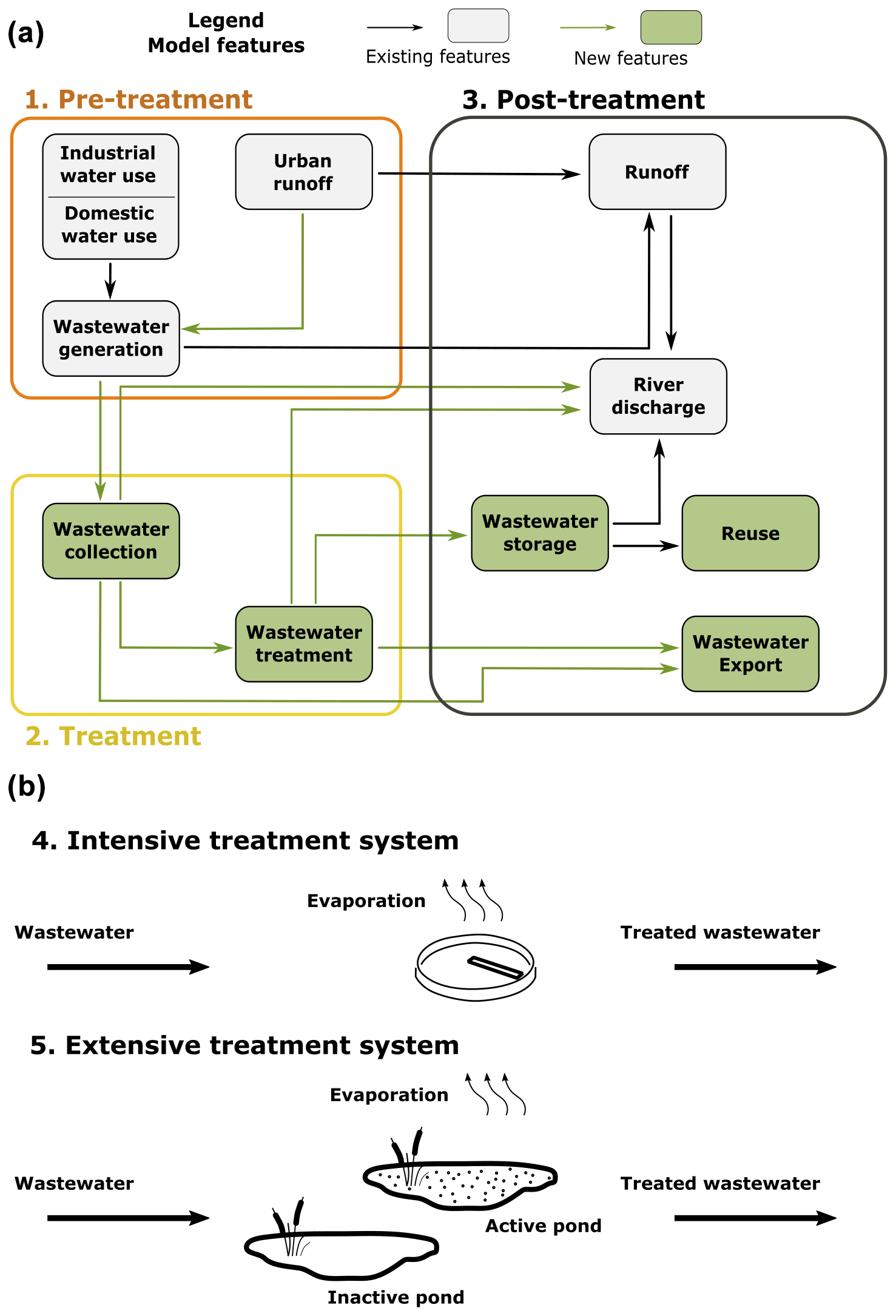
Figure 1 (a) The new features in WTRM (green boxes and arrows) and their interactions with the existing features of CWatM (gray boxes and arrows). (b) Water balance for the intensive and extensive wastewater treatment systems.

2.2.1 Pre-treatment: wastewater generation and collection

Wastewater generation in CWatM is represented by non-irrigation return flows, which are a function of water availability and sectoral allocation scheme, and the ratio between the consumptive and total water withdrawal. The wastewater module estimates domestic and industrial wastewater generation (Eff^Dom and Eff^Ind, respectively) by multiplying the non-irrigation return flows by the relative sectoral water demand. The next step is to collect and supply wastewater to wastewater treatment plants (WWTPs) (see Eq. 1).

Equation (1): calculating WWTP influents in WTRM.

WWTP influents in WTRM are calculated as follows:

$$\begin{array}{}\text{(1)}& \begin{array}{rl}{\text{Inflow}}_{j,t}& =\sum _{l\in j}({\text{Eff}}_{l,t}^{\text{Dom}}\times D_j^{\text{Dom}}+{\text{Eff}}_{l,t}^{\text{Ind}}\times D_j^{\text{Ind}})\times {\text{Cs}}_l\\ & +{\text{Rf}}_l\times \mathit{\alpha },\end{array}\end{array}$$

where j and t represent a simulated WWTP and the time step, respectively, and l indicates a grid cell. Table 4 describes all of the WTRM variables, data sources, and default values. WWTP service areas (or collection areas) are model input defining the linkages between the location of wastewater generation (individual grid cells, denoted by l) and wastewater treatment plants (denoted by j) – namely, that the wastewater from all grid cells in a collection area is treated at the associated WWTP (see Fig. S10). Wastewater collection is also a function of the sewer connection rate (Cs_l), where a value of 1 indicates that all wastewater is collected and sent to a WWTP. Moreover, it can include urban runoff (Rf_l) due to leakage or integration of the urban stormwater and wastewater systems. The α coefficient defines the system integration level and ranges from 0 (no integration) to 1 (complete system integration). The total wastewater collected in all grid cells l associated with a WWTP j is registered as the treatment plant's inflow.

Modeling sector-specific wastewater treatment at a WWTP (e.g., treatment of only industrial wastewater) is an advanced model functionality and currently does not fit a global application. It uses a Boolean variable (e.g., D^Dom), which equals 1 if the treatment plant receives a specific wastewater stream (e.g., domestic). A default value of 1 for both sectors is set in place in the case of missing data.

2.2.2 Treatment: influent, evaporation, and effluent

Simulated WWTPs must have the following basic features: location, start year of operation, daily treatment capacity, treatment period (days), and outflow location.

Currently, the module supports two optional wastewater treatment technologies associated with the treatment period. The two options are intensive and extensive treatment plants, as described in points 4 and 5 in Fig. 1b, respectively. Intensive treatment refers to conventional wastewater treatment technology and is characterized by a low residence time and low area requirements. It treats water to secondary or tertiary levels over less than 24 h (Pescod, 1992). CWatM uses a daily time step, so the intensive treatment plant's treatment period is set to 1 d. Any WWTP with a longer treatment period (i.e., ≥2 d) would be classified as extensive. Extensive treatment refers to natural biological systems that consist of a short primary treatment in a relatively deep anaerobic pond which is followed by a longer residence time (20–40 d) in a shallow facultative pond for secondary treatment (Pescod, 1992).

An advanced model feature enables the exceedance of the WWTP daily capacity by temporarily reducing the hydrological retention time (HRT). This feature is enabled by setting a treatment-plant-specific minimally allowed HRT, providing WWTPs some buffer to handle days with extreme inflows, e.g., due to rain events. Another advanced option is to simulate WWTP closure or upgrades by providing an end year of operation for a WWTP instance.

The main flows within the treatment section are influent, evaporation, and effluent, as described below.

Influent inflows

According to the basic model setup, excess wastewater beyond the plant's daily treatment capacity is discharged to a predefined outflow location (see Table 4). However, the model holds advanced modeling capabilities, enabling WWTPs to accept larger inflows to handle temporal fluctuations (e.g., due to significant rain events). Inflows higher than the designed capacity shorten the hydrological retention time (HRT or residence time), resulting in less effective wastewater treatment. The designed retention time is calculated as ${\text{HRT}}_j^{\text{Design}}={\text{Volume}}_j/{\text{Inflow}}_j^{\text{Design}}$, where Volume_j is the volume of WWTP j and ${\text{Inflow}}_j^{\text{Design}}$ is the daily treatment capacity of WWTP j (Pescod, 1992). The daily treatment capacity and time (or designed HRT) are model inputs (see Table 4). The minimally allowed HRT (days) parameter allows treatment plants to maintain higher inflows than their designed capacities. It expresses the lowest operational hydraulic retention time that a treatment plant can withstand before it refuses inflows. Following the calculation of the hydraulic retention time, the maximum daily capacity can be calculated as follows: ${\text{Inflow}}_{\text{max}}=\text{Volume}/{\text{HRT}}_{\text{min}}$, where Volume is fixed. For example, a minimally allowed HRT of 0.8 d implies an increase of 25 % in the operational daily capacity for a designed treatment time of 1 d.

Evaporation

Water surface evaporation is calculated by multiplying the potential open-water evaporation rate by the treatment pools' estimated surface area, and the pools' live storage volume limits it. Calculating the surface area of the treatment pools is different for intensive and extensive systems. The surface area of an intensive WWTP is defined as the ratio between the plant volume and the pool depth. For that purpose, a simplified representation of a WWTP treatment pool is adopted based on a clarifier design (used during both primary and secondary treatment; Pescod, 1992), and the pool depth is estimated to be 6 m (WEF, 2005; see Fig. B1).

Extensive systems are modeled as natural biological treatment ponds, alternately filling up and treating water. These processes consist of a relatively short anaerobic treatment in deeper ponds that is followed by a long-term (20–40 d) residence in facultative shallow ponds (see Fig. 1b; also refer to Pescod, 1992). Unlike intensive systems, treatment ponds in extensive systems may remain empty for long periods. As evaporation is simulated at the pond level, it considers only ponds with positive water storage.

Equation (2): calculation of the surface area of extensive treatment systems.

The surface area of extensive treatment systems is calculated as follows:

$$\begin{array}{}\text{(2)}& {\text{As}}_j={\displaystyle \frac{\mathrm{1}}{{\text{Depth}}_j}}\times \left({\text{VolCap}}_j\times {\displaystyle \frac{{\text{TreatTime}}_j}{{\text{TreatPool}}_j-\mathrm{1}}}\right).\end{array}$$

The surface area of each treatment pool is calculated by dividing the pool's volume by its depth (see Eq. 2; Depth is currently set to 1.5 m, as the depth of a facultative pond; Pescod, 1992). Each pool's volume is derived by multiplying the daily capacity (VolCap) by the pool's filling time. The latter is a function of the designed treatment time (TreatTime) and a predefined number of treatment pools (TreatPool; currently set to two; Pescod, 1992). Although evaporative losses are generally small (see Fig. 4), we allow modelers to change these default technical values to their estimates (see Appendix B).

Effluents

Treated wastewater (effluent) is discharged into a natural waterbody or sent to reservoirs for reuse. The timing of effluent release differs between intensive and extensive systems. Figure 1b shows the main differences between these two types of systems. In intensive systems, influents remain in the treatment plant throughout the predefined treatment time. For example, for a treatment time of one time step, the effluent volume at time t equals the influent volume minus the evaporation of time t – 1.

Extensive systems differentiate between two types of treatment ponds. At each time, one treatment pond receives all inflows; the other pond is either full or empty. Ponds that do not receive inflows and are not empty are considered “active”, i.e., wastewater treatment occurs. Effluents are released from active ponds under either of the following conditions: (a) a predefined treatment time has passed since the active pond stopped receiving inflows or (b) all pools are at full capacity and more influents should be added into the system. In the latter case, the effluents always originated from the active pond that had gone through the longest treatment time, although they may not be fully treated.

2.2.3 Post-treatment

The basic module has two post-treatment options: river discharge and reuse. Direct reuse (e.g., for irrigation, industrial, and potable applications) is possible using the CWatM reservoirs and water demand routines. This option requires data on the linkages between WWTPs and reservoirs, representing existing or planned water conveyance systems. The routine iterates over the list of WWTP-reservoir links and attempts to send treated wastewater to associated reservoirs. In the case of multiple recipient reservoirs, the water is split in proportion to the reservoirs' remaining storage (calculated as ${\text{remainingStorage}}_{i,t}={\text{totalVolume}}_i-{\text{liveStorage}}_{i,t}$). Excess water is discharged to predefined overflow locations if all related reservoirs are full. Discharge into streams/rivers is the default behavior if no reservoir is associated by a treatment plant. Finally, untreated wastewater is discharged if a plant's inflows exceed the plant's peak capacity (see the minimally allowed HRT in Sect. 2.2.2).

Treated wastewater can be managed in a separate reuse system by establishing a set of artificial, off-stream (type-4) storage reservoirs. A type-4 reservoir is not connected to the river network and, thus, has no channel-related inflows or outflows. Instead, water inputs include water/wastewater pumping, whereas water outputs are evaporation and pumping. The model combines the two approaches mentioned above, as each WWTP can be linked to one or more reservoirs or can discharge its water directly into a river channel. Indirect reuse can be simulated by releasing the water into a channel; upstream to a lift area, where river water is abstracted and used; or into a reservoir linked to the river network, where effluents are mixed with fresh water.

The module is designed to allow interbasin transfers of wastewater or treated wastewater, although this advanced option is not required in the case of a global model. Interbasin transfer of treated wastewater aims to account for cases in which the reuse areas extend beyond the borders of the simulated river basin. In that case, WWTP-specific export-share parameters indicate the daily fixed percentage of treated wastewater transferred for reuse in other basins. Similarly, the interbasin transfer of untreated wastewater represents cases in which treated wastewater collected in one basin is treated in another. This occurs automatically if a defined service area is not associated with any WWTP within the simulated basin.

3 Case study application

Israel is located on the eastern coast of the Mediterranean between the latitudes of 29 and 34° N and along the 35° E longitude. Its central coastal and northern regions are governed by a Mediterranean climate (hot and dry summer), its eastern areas are arid due to the rain shadow from its central mountain range, and the southern regions experience a semi- to hyperarid climate due to their vicinity to the world's desert belt.

During the 1960s, Israel initiated a country-wide water conveyance system (the “National Water Carrier”) to transfer water southwards from the northern Sea of Galilee, allowing rural development and large-scale irrigation in the semiarid Negev region (Tal, 2006). Presently, Israel's water system is intensively managed and relies primarily on seawater desalination, treated wastewater reuse, and groundwater abstraction. Although it is a nationally managed system, significant regional differences exist in sectoral water provision (Fridman et al., 2021).

The Ayalon Basin is located in Israel and the West Bank and stretches 815 km² between the western slopes of the Judaean Mountains and the Mediterranean coastal zone. A few kilometers inland, the Ayalon River spills into the Yarkon (see Fig. 2). Ayalon is an urbanized river basin partially overlaying the Tel Aviv metropolitan area downstream and the city of Modi'in-Maccabim-Re'ut in its middle segment. Downstream urban areas result in considerable water demand, vast runoff from sealed areas, and a high rate of wastewater generation. Upstream, the landscape of the Ayalon Basin is predominantly a rural mosaic of open areas and small settlements. Patches of irrigated agriculture and forests are primarily found in the southeastern parts of the basin.

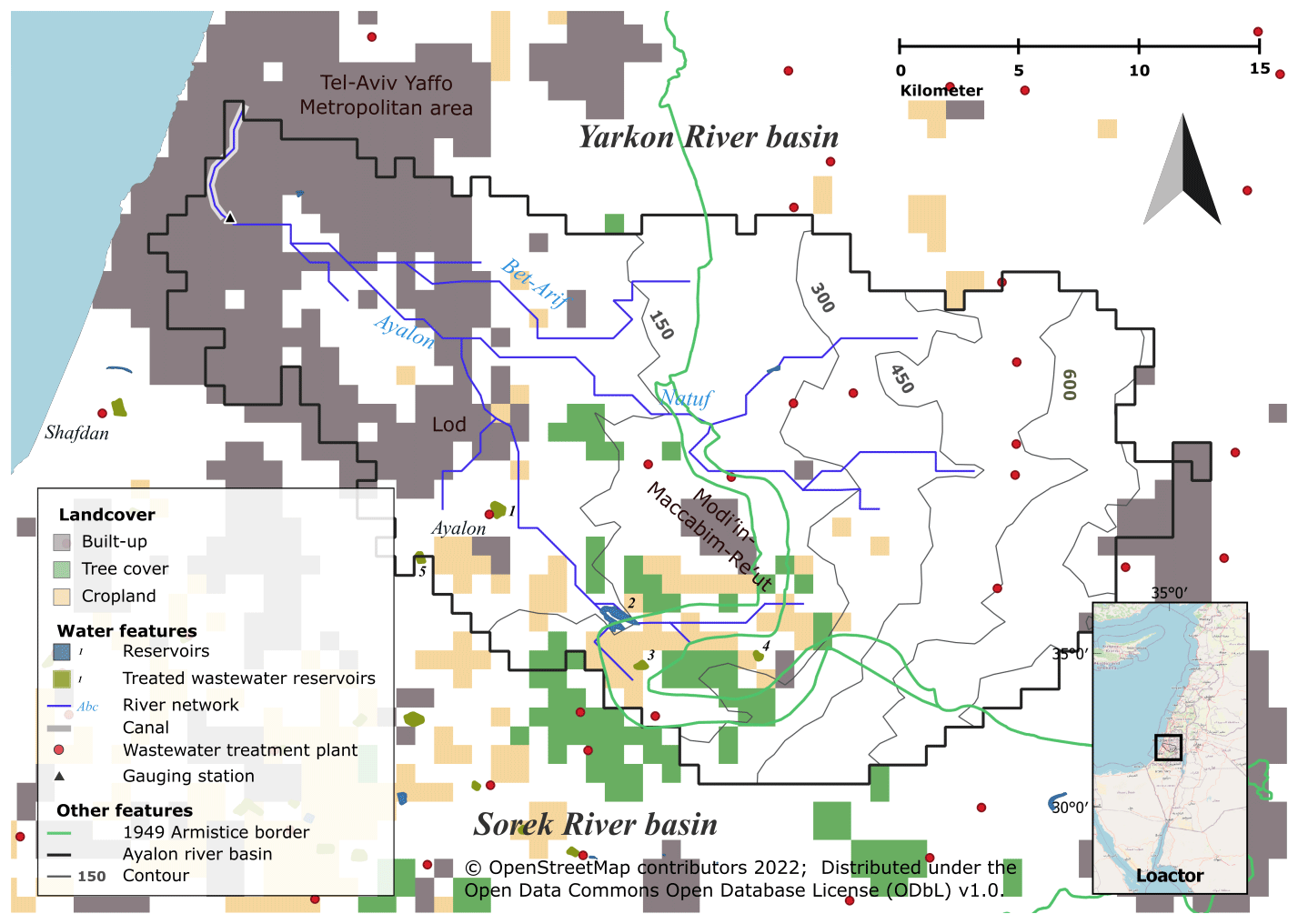
Figure 2 The Ayalon Basin case study: land cover and significant water features. Partially uses data from © OpenStreetMap contributors 2022. Distributed under the Open Data Commons Open Database License (ODbL) v1.0. The marked reservoirs are as follows: (1) Ayalon, (2) Mishmar Ayalon, (3) Ta'oz, (4) Mesilat Zion, and (5) Matsli'ah. Publisher's remark: please note that the above figure contains disputed territories.

Ayalon is a seasonal river originating in the southeastern part of the basin. An artificial “horseshoe-shaped” reservoir (“Mishmar Ayalon”) regulates its flows and maintains relatively fast groundwater recharge. Five main tributaries drain the remaining basin and feed the Ayalon River downstream. An artificial, cemented canal collects the river water before crossing densely populated urban areas downstream.

3.1 Data sources

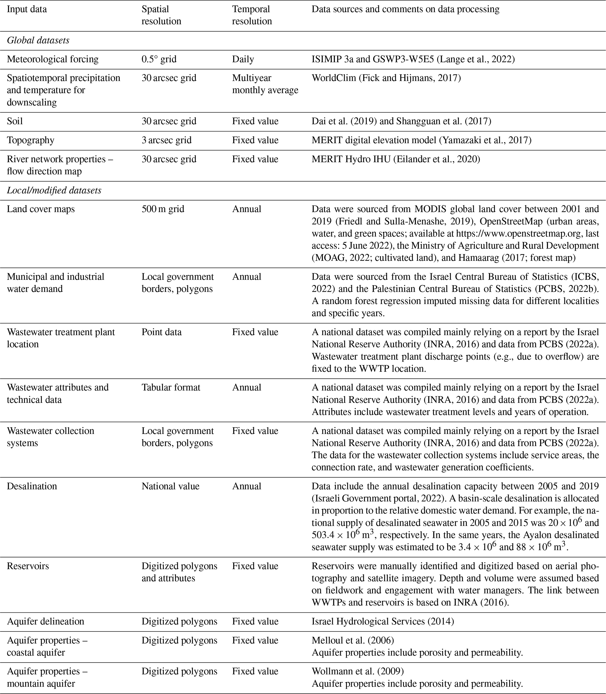
CWatM provides global datasets at a 0.5° and 5 arcmin resolution, as described in Burek et al. (2020). This high-resolution analysis better combines global and local data sources to represent the case study hydrologic processes and human–hydrologic interactions (Hanasaki et al., 2022). Table 1 provides an overview of both the global (e.g., meteorological forcings, soil characteristics, topography, and the river network) and the local (e.g., wastewater treatment and reuse, reservoir networks, aquifer properties, land cover maps, seawater desalination, and water demand) datasets. A complete documentation of the dataset associated with this publication is available at https://doi.org/10.5281/zenodo.12752966 (Fridman et al., 2025).

Table 1 Model inputs from global and local datasets. Unless explicitly indicated, all datasets were resampled to 30 arcsec or converted to a raster format.

3.1.1 Groundwater basins and aquifers

This case study uses the coupled CWatM–MODFLOW6 model to account for the interface between surface and groundwater hydrology and groundwater dynamics (Guillaumot et al., 2022). The Ayalon Basin lies above two principal groundwater aquifers. The Western Mountain Aquifer is part of the larger Yarkon-Taninim Aquifer system and has two partially separated sub-aquifers reaching a thickness of 600 m. It comprises carbonate sedimentary rocks and has a relatively high but non-homogenous hydraulic conductivity (Wollmann et al., 2009). The slopes of the western Judaean Mountains function as recharge zones, and the top layers in the western foothills are made of chalk and marl and act as an aquitard, confining the Western Mountain Aquifer (see Fig. A1). To the west, the relatively shallow coastal aquifer (thickness up to 200 m) mixes a sandstone aquifer with a clay lens, resulting in varying hydraulic conductivity (Melloul et al., 2006). Data on groundwater abstraction volumes, locations, and the water table changes were unavailable.

3.1.2 Reservoirs

We manually identified and digitized reservoirs in the Ayalon Basin using multiple data sources, including georeferenced aerial photography, visual inspection of satellite imagery, fieldwork, and interviews with local water management experts. The biggest reservoir in the Ayalon Basin is Mishmar Ayalon (7.5×10⁶ m³; Fig. 2), a seasonal water storage fed by the upstream section of the Ayalon River that regulates downstream flows. The Natuf reservoir is located at a former quarry site northeast of the basin (4.3×10⁶ m³) and contributes to groundwater recharge. Four smaller reservoirs constitute the wastewater irrigation infrastructure and have a total designed storage of 634 200 m³. This reuse system extends beyond the basin's borders, and we account for this by exporting a fraction of the treated wastewater.

3.1.3 Wastewater in the Ayalon Basin

Two primary WWTPs collect the wastewater generated in the main cities, and small-scale treatment plants collect that generated by the rural sector. The Shafdan WWTP treats all wastewater generated in the Tel Aviv metropolitan area in the adjacent Sorek River basin, which is outside the scope of this analysis. Later, this water is exported to northwestern Negev for irrigation purposes (Fridman et al., 2021). The Ayalon WWTP is the most significant facility in the basin, with a daily capacity of 81 000 m³. It collects treated wastewater from the cities of Lod and Modi'in-Maccabim-Re'ut (see Fig. 2) as well as their surrounding areas. An extensive treatment plant has existed since 1995, but development and population growth have exceeded its capacity, increasing sewer discharge frequency into the stream. An intensive activated sludge treatment plant with a daily capacity of 54 000 m³ started operating in 2003. However, on some occasions, daily inflow exceeded daily capacity by over 1.5 times (see Table S4). Almost 10 small-scale wastewater treatment plants in the Ayalon Basin are treating sewage at a settlement scale with a total daily capacity of 12 298 m³.

3.2 Setting calibration scenarios and model parameters

In this analysis, we simulate the Ayalon Basin hydrology and wastewater treatment and reuse under three scenarios, aiming to explore the effects of the wastewater treatment module's different modes of operation on model calibration and basin-scale water resource management. In the first scenario (S0), we disable the wastewater treatment and reuse module. The second (S1) and third (S2) include wastewater treatment and reuse without and with urban runoff collection, respectively. The share of urban runoff flowing into the sewers is set as a calibration parameter in S2. In this case study, we defined sectoral water allocations to limit wastewater reuse to irrigation, with limited use for livestock purposes. Additional calibration parameters are associated with the evapotranspiration rates of irrigated cropland and grassland, soil depth adjustment, the within-grid-cell soil moisture spatial distribution, the soil hydraulic conductivity and water content at saturation, Manning's roughness coefficient, the riverbed exchange rate, the urban evaporation coefficient, and the urban infiltration coefficient. The emphasis on the urban landscape is due to the relatively high share of built-up areas in the Ayalon Basin (see Fig. 2).

We set three more wastewater reuse scenarios apart from the calibration scenarios by expanding the irrigated agriculture area (by 2.5 %) and increasing storage volume (by 5 %) for two reservoirs for which command areas are defined: Ayalon and Matsli'ah. One scenario includes expansion and increased storage, and each of the other scenarios includes expansion or increased storage.

4 Results

4.1 Model validation

We have calibrated the Ayalon case study against the daily average discharge at the Ayalon-Ezra gauging station (32.04° N, 34.794° E; Fig. 2) over the period from 1 August 2001 to 30 July 2006, whereas validation was carried out over the period from 1 August 2007 to 31 December 2019. We further compared the simulated evapotranspiration with multiple satellite-derived products (Fig. S7; Mu et al., 2014; Reichle et al., 2022; Rodell et al., 2004) and the simulated monthly influent flows into the Ayalon WWTP with observed data between 2016 and 2019 (Fig. 5; Ayalon Cities Association, 2020, 2021, 2022, 2023). We measure model performance using the Kling–Gupta efficiency (KGE) and Nash–Sutcliffe efficiency (NSE) coefficients (Moriasi et al., 2015).

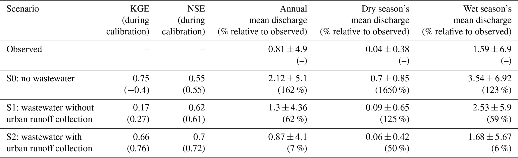
The S2 (wastewater and urban runoff collection) scenario generated the best-performing model (KGE=0.76 and NSE=0.72 during training), followed by S1 (wastewater without urban runoff collection; KGE=0.27 and NSE=0.61), and S0 (no wastewater; $\text{KGE}=-\mathrm{0.4}$ and NSE=0.57). Model performance was lower during the validation periods across all scenarios. During the validation periods, the complete implementation in scenario S2 also resulted in the best-performing model (${\text{KGE}}_{\mathrm{2006}-\mathrm{2013}}=\mathrm{0.69}$ and ${\text{KGE}}_{\mathrm{2014}-\mathrm{2019}}=\mathrm{0.55}$). Over the complete simulation period (1995–2019), the mean observed discharge at the outlet was 0.81 m³ s⁻¹, and it was best matched by the simulated discharge in scenario S2 (0.87 m³ s⁻¹; see Table 2). The full implementation scenario (S2) best matches the observed discharge during most days in the dry (April–September) and the wet season, as demonstrated in Fig. 3b. Sometimes, the model overestimates discharge or simulates flow events during the dry period (e.g., late April 2003; see Fig. 3c). This overestimation is often associated with a mismatch between forcing data (e.g., precipitation) and actual precipitation (see Fig. S6 and Table S1 in the Supplement). The S2 scenario performs well and captures peak events better when compared to the alternative modes of operation. For example, it overestimated the discharge in a peak flow event at the end of February 2003, whereas others underestimated the discharge by over 50 % (see Fig. 3a and b).

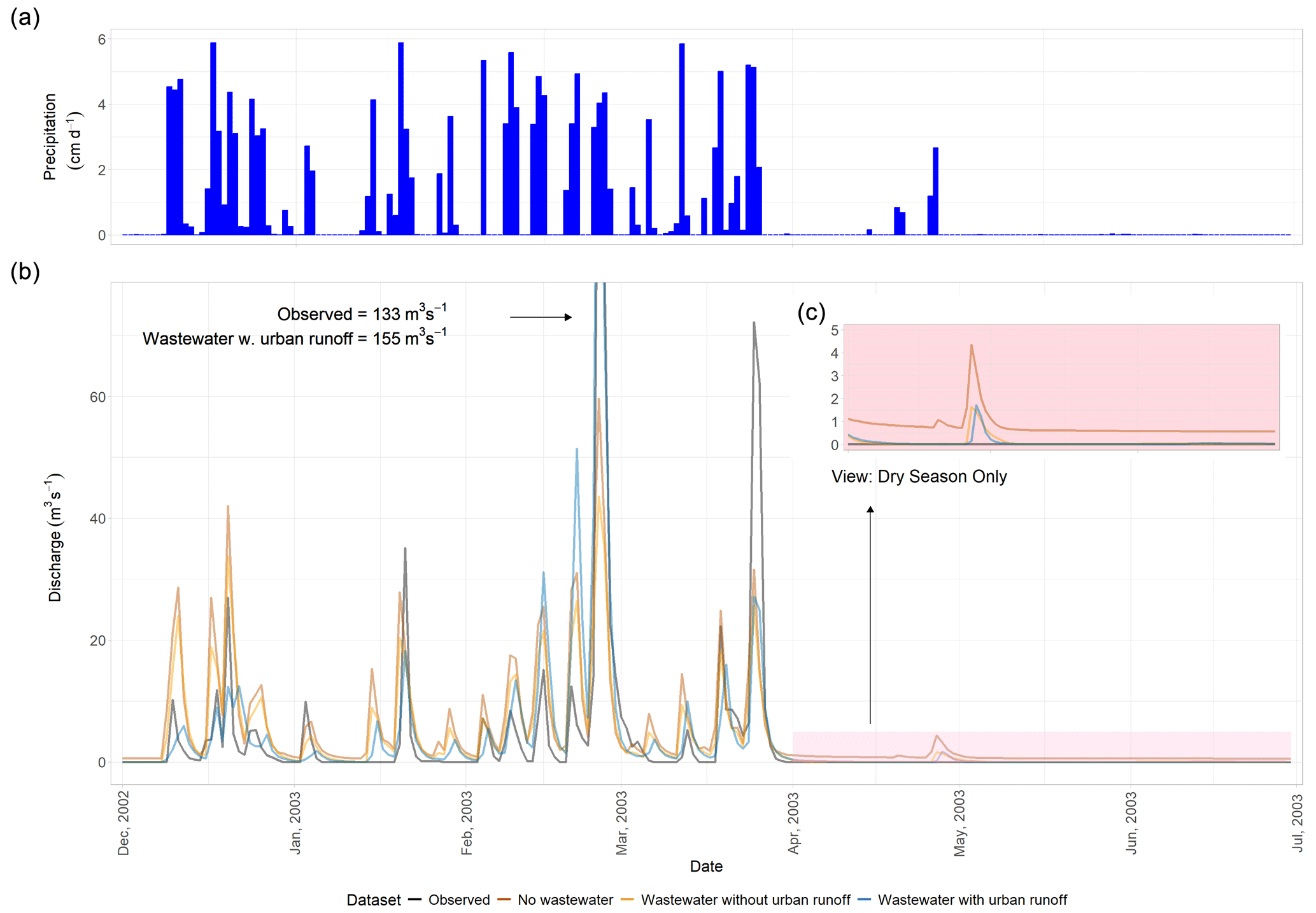
Figure 3 (a) Daily average rain depth in the Ayalon Basin and (b) observed and simulated discharge at the outlet between December 2002 and July 2003. (c) A zoomed-in view of the observed and simulated discharge in the dry season.

The simulations were compared with different remote-sensing-derived evapotranspiration (RS-ET) time series. All scenarios can capture seasonal dynamics but overestimate ET during early spring (around March–April, except SMAP; see Fig. S7). The “no wastewater” (S0) scenario highly overestimates the ET, whereas the other two (S1 and S2) scenarios better align with the RS-ET data, particularly after 2015. There are differences between the RS-ET datasets associated with process, forcings, and parameterization errors (Zhang et al., 2016); some are shown in Table S2. GLDAS-2.1 shows the lowest KGE across scenarios, whereas SMAP indicates the highest (see Table S3). These findings are consistent with an intercomparison of RS-ET datasets (Kim et al., 2023). Furthermore, activating additional features of the wastewater module improves the simulated ET trends compared with RS-ET datasets. The average KGE values are −0.68 (S0), −0.27 (S1), and −0.17 (S2).

Modeling the intermittent Ayalon River case study is challenging, mainly due to its arid climate and small basin area. Under these conditions, even a small deviation in the absolute simulated discharge results in a high relative error. It follows that diverting return flows (i.e., sewage) away from the river was a crucial step in the Ayalon model calibration. Introducing wastewater treatment and reuse into CWatM enables the simulation of actual water dynamics in the Ayalon Basin, resulting in a better-performing model. The respective KGE values of scenarios S0, S1, and S2 between 1995 and 2019 are −0.75, 0.17, and 0.66, and the percentage differences between the simulated and observed average discharge are 162 %, 62 %, and 7 %, respectively (see Table 2). Similar improvement is also shown when comparing simulated and observed discharge between 1995 and 2019 (see Figs. S1–S3 in the Supplement). The improvement due to including the wastewater treatment and reuse module (scenario S1) is associated with reducing the dry season's baseflow from an average of 0.07 to 0.06 m³ s⁻¹. The effects of urban runoff collection were mainly evident in the wet season's discharge, which was reduced from an average of 2.53 m³ s⁻¹ (scenario S1) to 1.68 m³ s⁻¹ (scenario S2). The collection of urban runoff into the sewers reduces flows downstream to urban areas and fits, to some extent, the inflow dynamics into the Ayalon WWTP (see Fig. 5).

Table 2 Model performance under different scenarios over the complete simulation (1995–2019). The dry season occurs from April to September.

4.2 Component and flows of the wastewater module

The wastewater flows between different model components are illustrated in Fig. 4 using the water circle concept. A water circle is a simplified depiction of the water cycle within a specific region, component, and time frame. It illustrates the water balance by linking inputs, outputs, and changes in storage while also representing various water sources and uses (Smilovic et al., 2024). Figure 4 presents the wastewater reuse water balance in the Ayalon Basin between 2001 and 2006, totaling 209×10⁶ m³ yr⁻¹ (inputs + outputs + change in storage). Inflows to wastewater treatment plants primarily originated from non-irrigation return flows (labeled as 1 in Fig. 4), consisting mainly of domestic sewage mixed with urban runoff, especially in dual-purpose urban drainage systems. These inflows are based on existing model routines (e.g., water demand and soil; see Fig. 1a) and amount to 104×10⁶ m³. In the Ayalon Basin case study, the largest share (almost 70 %) of the influents is treated in the Shafdan WWTP outside of the basin of interest (labeled as 2 in Fig 4), while approximately 14 % is sent to reservoirs for reuse, although actual reuse is lower (labeled as 4 in Fig. 4). The gap between the volume of wastewater sent to reservoirs and the actual reuse is associated with evaporation, outflows, and leakage losses (prominent in one of the reservoirs; see Fig. S4). The remaining share includes the discharge of treated wastewater (4 %) and raw sewage (8 %; labeled as 4 in Fig. 4). Evaporative loss from WWTPs is marginal (<4 %) and is represented by one of the unlabeled wedges on the wastewater circle (labeled as 5 in Fig. 4).

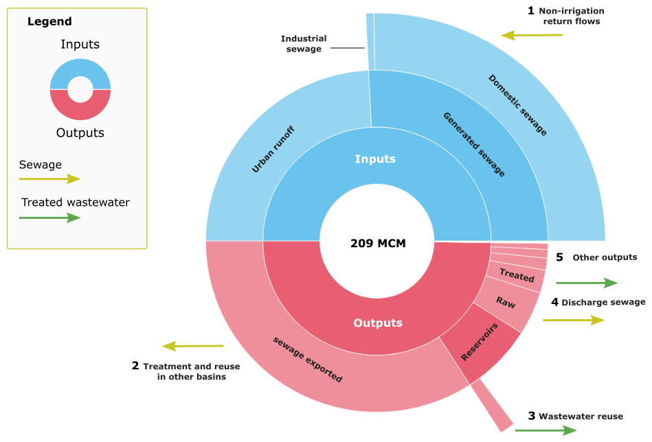
Figure 4 Average annual sewage and treated wastewater flows within and between CWatM model components (see labels 1–5), based on a simulation for the Ayalon Basin, Israel, from 1 January 2001 to 30 July 2006.

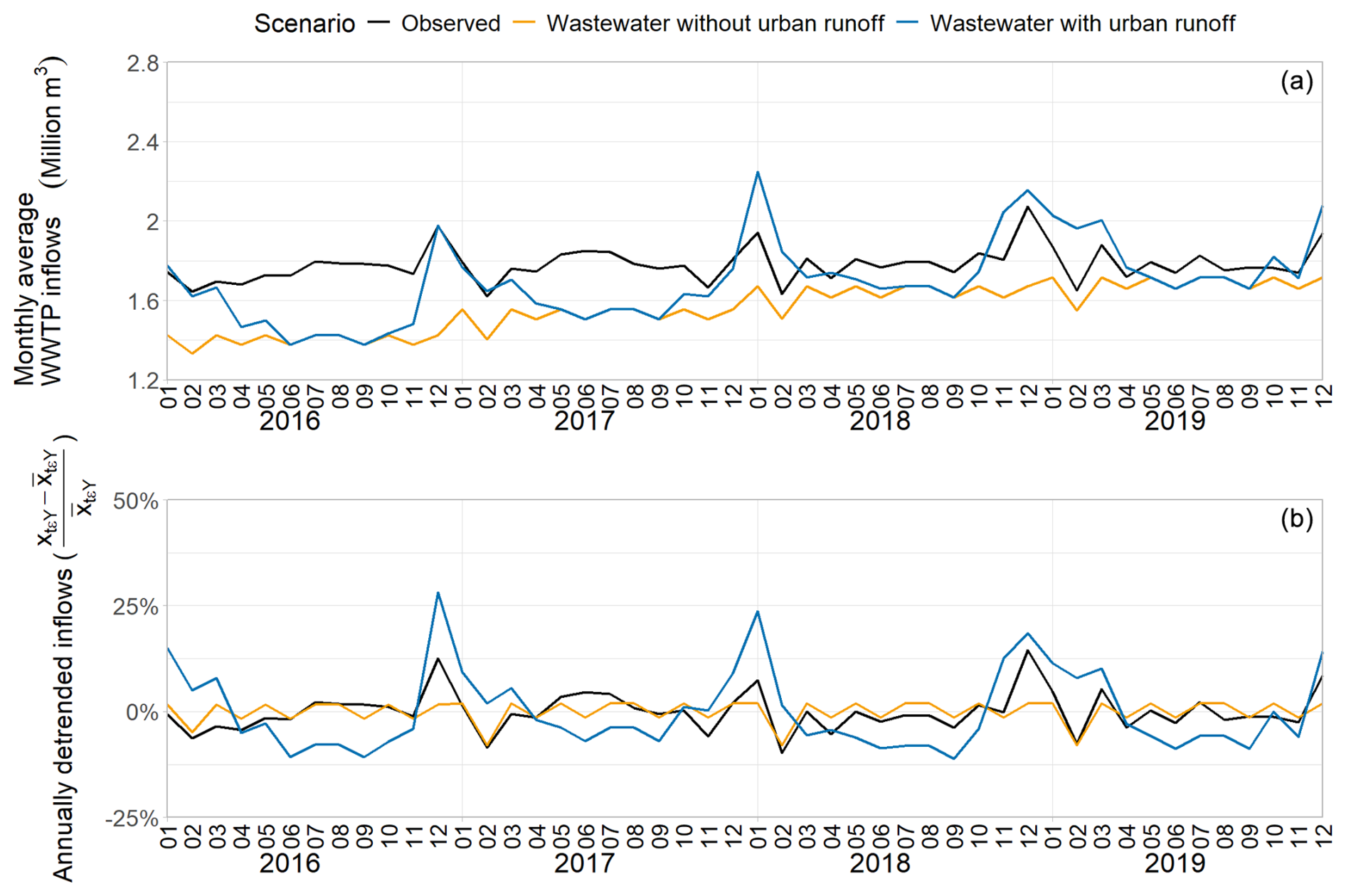
Figure 5 Observed vs. simulated monthly wastewater inflows into the Ayalon WWTP with and without urban runoff collection using absolute values (a) and annually detrended values (b) (Ayalon Cities Association, 2020, 2021, 2022, 2023).

The annual average wastewater reuse in the Ayalon Basin (2.3×10⁶ m³) accounts for almost 10 % of the basins' irrigation withdrawal (25×10⁶ m³). In addition, around 71×10⁶ m³ of the wastewater generated in the Tel Aviv metropolitan area (see Fig. S10) ia treated in the Shafdan WWTP (in the Sorek River basin) and reused for irrigation in southern Israel (Fridman et al., 2021).

4.3 Modeling wastewater and urban stormwater collection systems

CWatM includes two main hydrological processes for urban areas: return flows (e.g., sewage generation) and urban runoff. These flows are managed by either separated or combined collection and drainage systems. In Israel, two systems are operated separately to collect urban wastewater and stormwater. However, stormwater frequently leaks into the sewers due to illegal urban drainage connections.

The runoff collection coefficient allows the user to control the magnitude of system integration. One combined system would have a coefficient of 1, implying that all urban runoff flows into the sewers collection system, whereas a coefficient of 0 suggests two completely separated systems. The calibrated model ended up with a coefficient of 0.78, implying that 78 % of urban runoff flows into the sewers.

The advantages of the runoff collection coefficient are shown in Fig. 5, which compares the monthly inflows to the Ayalon WWTP against the simulated inflows with (S2) and without (S1) urban runoff collection. On average, between 2016 and 2019, the Ayalon WWTP accepted $\mathrm{1780}\pm \mathrm{86}\times {\mathrm{10}}^{\mathrm{3}}$ m³ of sewage every month. The average inflows in the scenarios without and with urban runoff collection are 1562±119 and $\mathrm{1699}\pm \mathrm{203}\times {\mathrm{10}}^{\mathrm{3}}$ m³ per month, respectively. Overall, the model underestimates the inflow to the Ayalon WWTP, as shown in Fig. 5a, during the dry months (e.g., April–June), which is probably due to the use of annual model inputs for water withdrawal that do not capture seasonality. Seasonality is only captured by the “wastewater with urban runoff” (S2) scenario as a direct result of urban runoff collection. Another factor limiting WWTP inflows is the minimum allowed HRT, presented in Sect. 2.2.2. Sensitivity analysis implies that a 1 % change in the parameter value results in an average 0.23 % change in the WWTP inflows (see Fig. S9 in the Supplement).

Rain events during the wet season often result in increased inflows to WWTPs (e.g., during December 2016 or January 2018). The scenario that includes urban runoff collection (S2) can simulate these peaks, although it slightly overestimates them, whereas no peaks are simulated for scenario S1, where no urban runoff is collected (see Fig. 5b). While it may be that the runoff collection parameter was set at a value that is too high, overestimating the peak flows can also result from errors in precipitation data (see Fig. S6). The wastewater with urban runoff collection (S2) scenario outperforms the scenario without wastewater collection based on multiple parameters (showing lower bias and a higher NSE and correlation; see Table S5).

4.4 Modeling of wastewater reuse potential and impacts

Wastewater treatment and reuse may significantly affect water management, particularly for complex water resource systems in water-scarce countries. Israel is a water-scarce country that reuses wastewater, utilizes desalination water, and transfers water between river basins to mitigate water stress. As Israel manages water nationally, analyzing water resources on a basin scale aligns differently compared with Israel's actual state of water resources. Instead, the following scenarios aim to illustrate the relevance of the WTRM module to water resource management.

Until the early 2000s, the Ayalon Basin's water supply relied primarily on groundwater abstraction. As a result of population growth and the expansion of the Ayalon WWTP's daily treatment capacity in 2003 (from 22 000 to 54 000 m³ d⁻¹), the simulated wastewater reuse has nearly doubled, increasing from 1.5×10⁶ m³ in the year 2000 to 2.7×10⁶ m³ in 2005. In the same year, desalinated seawater was first supplied, satisfying approximately 3 % of the total water demand in the basin. Over the years, the role of desalination has increased, accounting for around 47 % of the water supply. The share of treated wastewater slightly increased, reaching 2.7 % (approximately 3×10⁶ m³), compared with 1.5 % in 2000. Most importantly, avoided groundwater pumping in 2010 enhanced Israel's water security by reducing the pressures on aquifers, and the avoided seawater desalination reduced costs with respect to energy for water use and water production (Fridman et al., 2021).

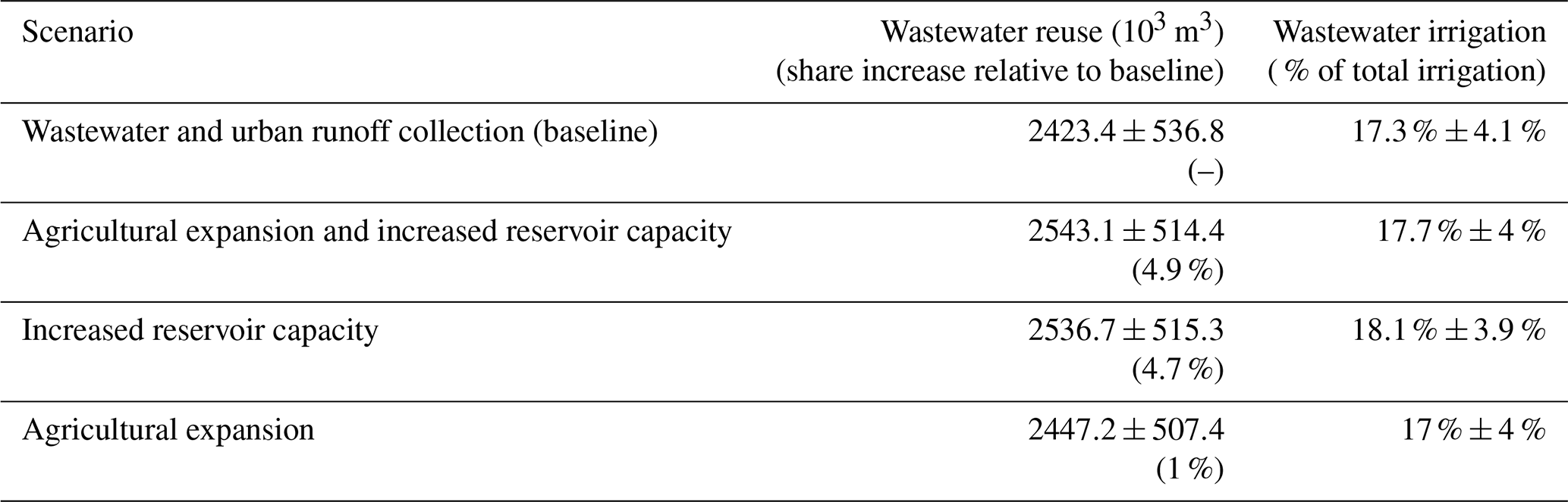
Focusing on irrigation districts linked to the Ayalon WWTP (see Fig. S11), Table 3 presents the multiyear average absolute and relative wastewater reuse (for irrigation) between 2000 and 2010. Overall, there is little difference between the baseline and agricultural expansion scenarios, showing a slight increase in the reuse volume but a slight decrease in the relative wastewater irrigation (relative to irrigation demand). These findings point out a balanced proportion between storage and water demand. Small access storage is maintained, allowing for additional irrigation to respond to increased water requirements. The two scenarios that include increasing storage demonstrate a higher wastewater reuse volume (4.7 %–4.9 %) and relative irrigation increasing from 17.3 % to 17.8 %–18.1 %. The share of wastewater reuse out of the total irrigation demand increased from around 13 % to 18 % in 2000 and 2003, respectively, and reached almost 25 % in 2006 (see Fig. S12). These changes were associated with an increased capacity of the Ayalon WWTP in 2003 and precipitation variability, e.g., lower irrigation requirements during wet years compared with a relatively constant supply of treated wastewater. As this reuse project extends southwards, outside the Ayalon Basin, the model also estimates additional wastewater reuse of almost 2×10⁶ m³ (i.e., treated wastewater sent for reuse outside the basin). In addition, more than 50×10⁶ m³ is collected and treated in the Shafdan WWTP, southwest of the Ayalon Basin (see Fig. 2), and is almost entirely reused.

Table 3 Average and standard deviation of the absolute and relative wastewater reuse in irrigation districts linked to the Ayalon WWTP between 2000 and 2010.

5 Discussion

5.1 Wastewater treatment and reuse play a crucial role in the hydrological modeling of urban watersheds, especially in low-discharge/intermittent rivers

Discharges from wastewater treatment plants often dominate urban watersheds' hydrological signals, increasing low flows, flashiness, and the frequency of medium- and high-flow events (Coxon et al., 2024). The effect of wastewater on stream hydrological signals would become more pronounced in intermittent streams, challenging model calibration. Acknowledging this fact, one may compromise on model performance in urban watersheds; however, including wastewater treatment and reuse in the modeling allows for increased model performance, as it better represents local water management processes. The example provided in this paper demonstrates this point by showing a significant increase in model performance due to including wastewater treatment and reuse in the modeling.

To our knowledge, only a few existing hydrological models account for wastewater treatment and reuse. DynQual, for example, simplifies the treatment process and only allows for indirect reuse; i.e., treated water is discharged into rivers and can be abstracted downstream. Moreover, the SWAT model represents wastewater treatment by including pit latrines. However, both models focus on the water quality and missing critical operations associated with water quantity (e.g., reuse through reservoirs or directly to fields). Although addressing the highly relevant topic of water quality, the representation of wastewater processes in these two models would not contribute to model calibration in urban or intermittent watersheds.

The importance of including wastewater treatment and reuse in high-resolution (i.e., ∼1 km) hydrological modeling is also aligned with recent findings, as these models are susceptible to the effects of human activity on the water cycle and often require better representation of these processes and more precise data (Hanasaki et al., 2022). It follows that the WTRM complements the recent shift towards high-resolution modeling at global (van Jaarsveld et al., 2025) and more local scales (e.g., CWatM implementation in Bureganland, Austria; Bhima Basin, India; and North China; Guillaumot et al., 2022; Yang et al., 2022).

5.2 The wastewater treatment module utilizes multiple features of CWatM, providing tools to conduct policy-relevant analysis on water resource management and wastewater treatment and reuse.

Wastewater is increasingly perceived as an untapped resource and is marked as a potential water source to reduce water stress or drought risk. Hydrological models, such as CWatM, are often used to inform decision-making and policies for enhancing water resource management and can benefit from WTRM capabilities.

The WTRM interacts with different existing modules and routines in CWatM, allowing the modeling of different wastewater reuse options. The source-sector abstraction fraction and reservoir operation options in CWatM are pivotal in modeling the treated wastewater reuse. The former is used to define the desired water mix, restricting wastewater reuse by some sectors (e.g., forbidding households from using treated wastewater). Reservoirs allow for the storage and transfer of treated wastewater and the reuse of it in relevant irrigation districts (i.e., by utilizing the CWatM command areas feature). Leakage from reservoirs into groundwater (see Fig. S4) can be used to simulate groundwater recharge with treated wastewater.

Indirect reuse is enabled when treated wastewater is released into a river channel or a reservoir, diluted, and later abstracted downstream, whereas direct reuse is mediated through a designated reservoir, disconnected from the river network (type-4 reservoirs). The inflows into this reservoir consist only of water transfers, and the outflows are limited to abstraction and evaporative losses. The water levels in these reservoirs are not affected directly by river flows and runoff, and they can maintain a traceable stock of treated wastewater over the long term. Abstraction from reservoirs occurs either within a certain buffer (i.e., defined by the number of grid cells) from the reservoir or within the area of an associated command area (area served by the reservoir regarding water supply). Combined with the source-sector abstraction fraction, the modeling of the Ayalon Basin has limited the use of treated wastewater for irrigation and, to a smaller extent, for livestock. Other existing uses, like urban landscaping or cooling of thermal powerplants, were excluded, as data were unavailable.

By utilizing these modules and processes, the paper explores the potential effects of the increased storage of wastewater reuse reservoirs and expanding irrigated agriculture areas. It focuses on the command areas associated with two reuse reservoirs (as indicated in Fig. S11), indicating a high share of irrigation with treated wastewater (∼17 %). The module variables could be utilized for exploring a wide variety of water management instruments, including using treated wastewater to mitigate drought risk (conveying and storing treated wastewater in high-drought-risk areas) – to recharge the aquifer (controlling reservoir infiltration rate) – or explore pathways for agricultural expansion/intensification. Wastewater reuse can also have economic or environmental benefits; the Ayalon case study is relevant for both due to potentially avoided seawater desalination, which is more expensive and requires more energy. Considering the nexus, economic, resource intensity, and emission data from different sources (e.g., life cycle assessments; see Liao et al., 2020; Meron et al., 2020) could complement such an analysis.

5.3 Flexible model design and available global datasets provide a robust starting point for simulating wastewater treatment and reuse scenarios at global-scale and coarser resolutions. Some data gaps remain and provide opportunities for scientific engagement

The Community Water Model, as well as other large-scale hydrological models (Hanasaki et al., 2022; Hoch et al., 2023), is shifting towards a multi-resolution modeling framework, allowing users to work on a global scale with coarser resolutions and on a local scale with higher resolutions. The need to better represent wastewater treatment and reuse in global, regional, and local hydrological modeling is linked to its increasing potential as a water resource. The WTRM provides diverse tools for including wastewater treatment and reuse in hydrological modeling. So far, the paper has focused on the module's advanced mode of operation, which is suitable for data-abundant regions or local case studies where data collection efforts are feasible. Nevertheless, applying the WTRM at a coarser (e.g., 5 arcmin) spatial resolution globally or in data-scarce regions requires a simplified workflow and a global data inventory.

Following the CWatM modular and flexible structure, the WTRM was developed with that notion in mind, facilitating a simple mode of operation with minimal data requirements but including advanced processes when data are available. The results presented and discussed show a significant increase in model performance as a result of a more straightforward implementation of the module (i.e., without urban runoff collection); this, along with the reuse scenarios, points to the potential impact of upscaling the analysis to cover other urbanized watersheds and water-stressed regions. The recent development of different global datasets provides an opportunity to upscale this analysis, although these data would have to undergo some processing to fit the CWatM data structure. Two such datasets are the HydroWASTE dataset (Ehalt Macedo et al., 2022) and that from Jones et al. (2021).

HydroWASTE is a global WWTP dataset describing plants' location, treatment level, operational status, population served, overflow discharge point, and daily capacity. It was recently used to determine the impact of droughts on water quality (Graham et al., 2024) and to account for the global microplastic fiber pollution from laundry (Wang et al., 2024). The dataset compiled by Jones et al. (2021) is a global gridded dataset (at a 5 arcmin resolution) describing wastewater generation volumes and collection, treatment, and reuse rates. These data have already been used to force global studies on water quality (van Vliet et al., 2021).

These two datasets provide sufficient global data at a spatial resolution of 5 arcmin to accommodate six of the seven mandatory variables required to set up a simple simulation (see Table 4). However, data are lacking for the year of establishment (or the start of operation) of a WWTP, which could be assumed by utilizing auxiliary time-series data, like drinking water sanitation and hygiene (WASH), available from the Joint Monitoring Program (JMP; https://washdata.org, last access: 12 March 2025), or sectoral outputs from monetary input–output tables (e.g., https://worldmrio.com, last access: 12 March 2025). These data could cast temporal trends of increased sanitation coverage or sectoral economic activity. Two additional challenges are indicated in Table 4, associated with the treatment days and service (wastewater collection) area. In this study, we rely on a national dataset associating municipalities with WWTPs (see Fig. S10; INRA, 2016), yet these data are not available for most countries. Instead, following Ehalt Macedo et al. (2022), the wastewater collection areas can be traced back from the WWTP to serve the nearest, most likely upstream, population centers. Treatment days are associated with the WWTP classification into intensive and extensive systems, which can be associated with the location and economic factors (like gross domestic product per capita or electrification status). The availability of such data at national, sub-national, and grid scales deems the classification of WWTPs as intensive or extensive and feasible.

Table 4 Model variables for simple and advanced simulations and potential data sources.

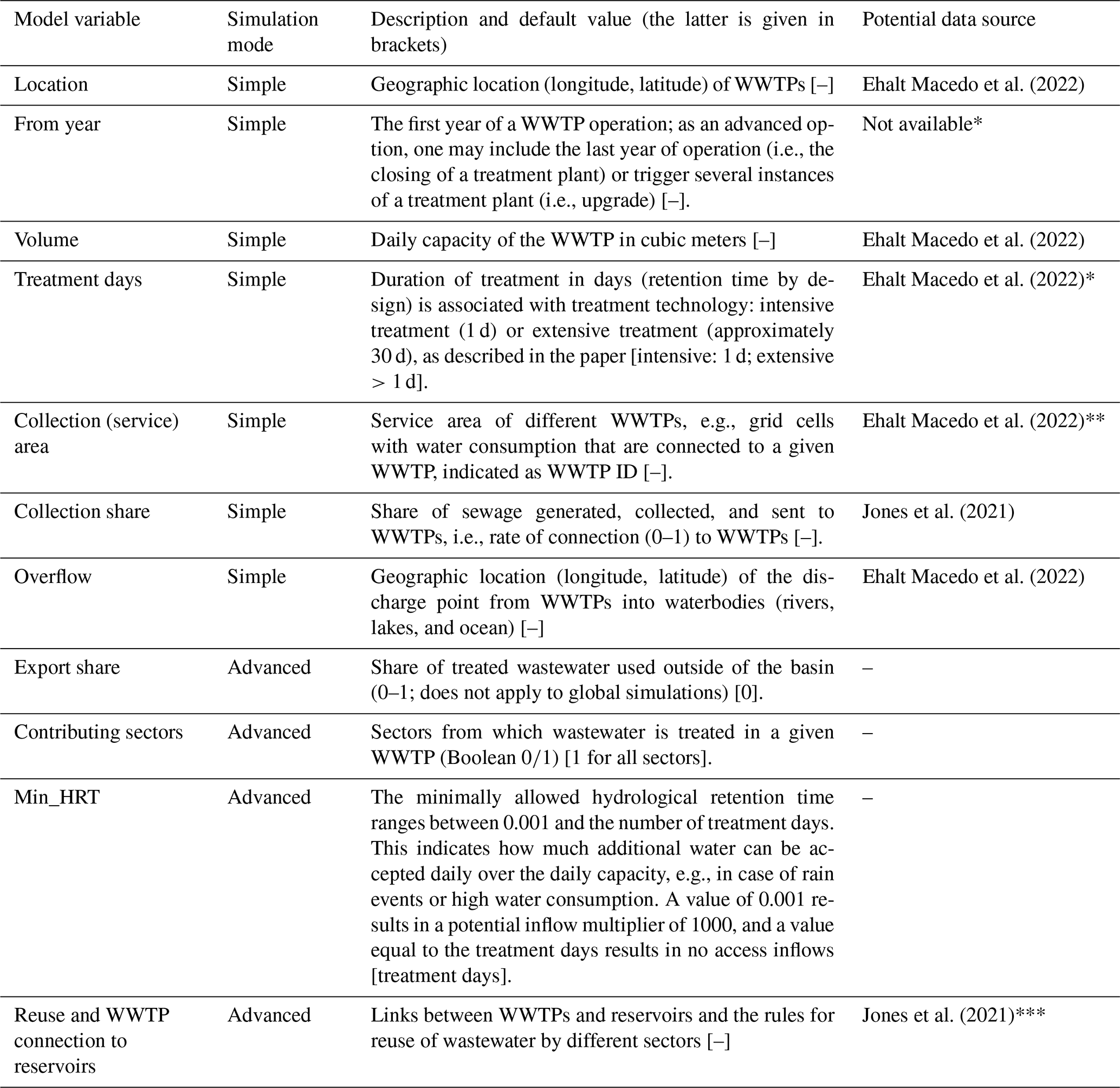
* The variable is unavailable but could be concluded by utilizing auxiliary data. ** The variable is unavailable but could be estimated based on published methods. *** Available data are highly uncertain at the grid scale and can be used to inform scenarios.

Advanced simulations are not pursued globally, so data sources for their required variables are not sought, except for reuse and reservoir connections, as reuse significantly impacts model performance and water resource management analysis. The reuse rates estimated by Jones et al. (2023) can be used for that purpose. However, as these estimations are not linked to any specific WWTP or reservoir, as required by the WTRM, this would require some pre-processing and simplifying assumptions. Some ongoing efforts to identify potential wastewater reuse for specific WWTPs can support this processing (Fridman et al., 2023), yet both data sources would involve high uncertainties at the grid scale. Two other approaches could be employed to assess different reuse scenarios, including indirect reuse from waterbodies (e.g., rivers and lakes) or the simulation of on-site type-4 reservoirs with command areas set as fixed buffers. Such reuse scenarios could be used to explore reuse by other non-agricultural sectors.

6 Conclusions

Wastewater primarily affects the hydrology in urbanized watersheds, particularly in water-stressed regions. Wastewater reuse can ease the pressure on natural water sources and reduce drought risk. However, large-scale hydrological models do not account for wastewater treatment and reuse. The recent trend towards higher spatial resolutions further emphasizes the need to include local data and processes in hydrological modeling.

This paper introduces a novel wastewater treatment and reuse module integrated into the large-scale multi-resolution Community Water Model. It provides a range of operational modes to balance modeling needs and data availability worldwide. A high-resolution case study of an urbanized and water-stressed watershed illustrated the WTRM's added value in terms of enhanced model performance and the inclusion of additional water sources, such as reused wastewater. The role of wastewater in water resource management planning can now be included in hydrological simulations, often used to inform such policies. Recently published global datasets were mapped to model variables, indicating that global modeling at a coarser spatial resolution (e.g., 5 arcmin) is also feasible. Some remaining data gaps, including the lack of time series or missing information on reuse projects, would require some assumptions and additional processing of input data. The compilation of a global input dataset is one desired future development. As wastewater is naturally associated with water quality, this aspect remains a limitation within the scope of the current development and would also be addressed in future developments.

Appendix A

Figure A1 describes the vertical and lateral permeability of the Yarkon-Taninim (YARTAN) and coastal aquifers in Israel. The coastal aquifer forms a relatively narrow stripe stretching north to the south. Next, the Western Mountain Aquifer is located towards the east, showing a relatively diverse permeability. The YARTAN groundwater basin includes the Western Mountain Aquifer but extends far beyond the borders of the Ayalon Basin.

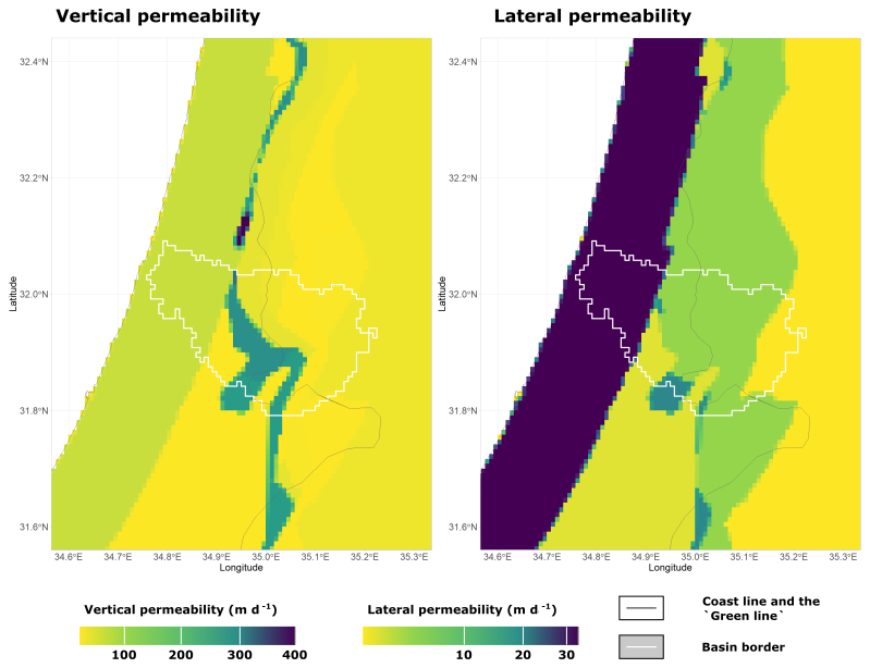
Figure A1 Vertical and lateral permeability in the YARTAN and coastal aquifers in the Ayalon Basin and its surroundings.

Appendix B

The treatment pool depth in an intensive WWTP represents the depth of a clarifier through which sewage flows at different treatment stages. The ratios between the clarifier's depth and diameter are relatively fixed to optimize the biological treatment of sewage (e.g., biofilm development). A standard design for a clarifier is a relatively deep pool with a sloped bottom, as demonstrated in Fig. B1. In the WTRM, the pool depth is only used to calculate the water surface area and simulate evaporative losses; therefore, we find a simplified representation of the treatment pool with a flat bottom sufficient. In Fig. B1, we convert the sloped-bottom clarifier dimensions (WEF, 2005) to the equivalent pool depth in a flat clarifier, maintaining the pool's volume. This results in an approximate depth of 6.6 m, which, based on data collected for the Ayalon case study, was rounded to 6 m. We allow modelers to change the pool depth of either intensive, extensive, or both treatment systems using the following settings in the settings file: “pooldepth_intensive” and “pooldepth_extensive”. The respective default settings are hard coded as 6 and 1.5 m, as described in this paper. In addition, to calculate the evaporation from extensive WWTPs, we allow users to change the default value of two treatment pools by adding the “poolsExtensive” to the settings file.

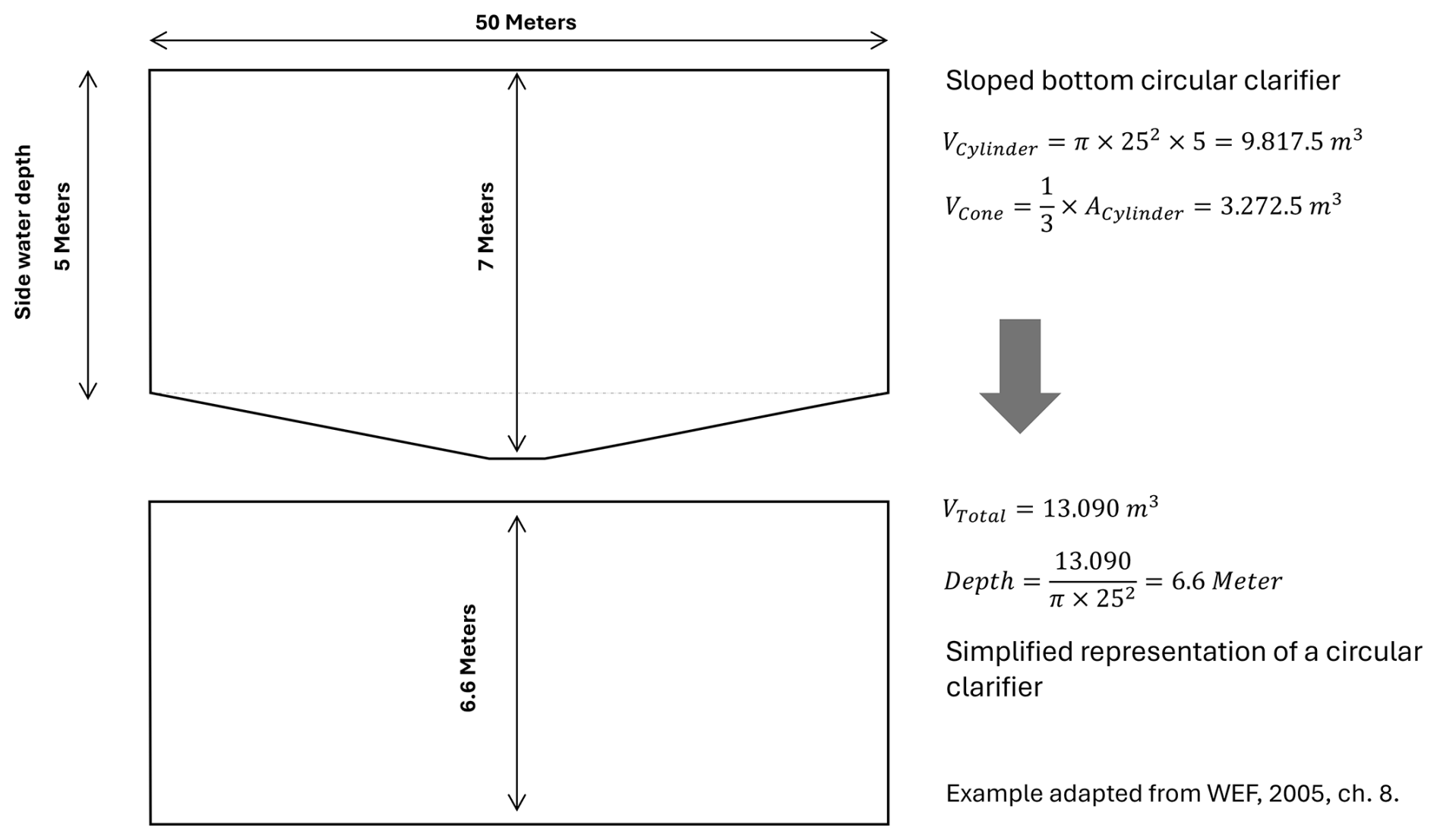
Figure B1 A simplified approach to estimate the wastewater treatment pool depth in an intensive WWTP.