Tuning the ICON-A 2.6.4 climate model with machine-learning-based emulators and history matching

In climate model development, “tuning” refers to the important process of adjusting uncertain free parameters of subgrid-scale parameterizations to best match a set of Earth observations, such as the global radiation balance or global cloud cover. This is traditionally a computationally expensive step as it requires a large number of climate model simulations. This step also becomes more challenging with increasing spatial resolution and complexity of climate models. In addition, the manual tuning relies strongly on expert knowledge and is thus not independently reproducible. To reduce subjectivity and computational demands, tuning methods based on machine learning (ML) have become an active research subject. Here, we build on these developments and apply ML-based tuning to the atmospheric component of the Icosahedral Nonhydrostatic Weather and Climate Model (ICON) at 80 km resolution. Our approach follows a workflow similar to other proposed ML-based tuning methods: (1) creating a perturbed parameter ensemble (PPE) of limited size with randomly selected parameters, (2) fitting an ML-based emulator to the PPE to generate a large emulated ensemble with the emulator, and (3) shrinking the parameter space to regions compatible with observations using a method inspired by history matching. However, in contrast to previous works, we apply a sequential approach: the selected set of tuning parameters is updated in successive phases depending on the results of a sensitivity analysis with Sobol indices. We tune for global radiative properties, cloud properties, zonal wind velocities, and wind stresses on the ocean surface. With one iteration of this method, we achieve a model configuration yielding a global top-of-atmosphere net radiation budget in the range of [0, 1] W m⁻², and global radiation metrics and water vapour path consistent with the reference observations. Furthermore, the resulting ML-based emulator allows us to identify the parameters that most impact the outputs that we target with tuning. The parameters that we identified to be mostly influential for the physics output metrics are the critical relative humidity in the upper troposphere and the conversion coefficient from cloud water to rain, influencing the radiation metrics and global cloud cover, together with the coefficient of sedimentation velocity of cloud ice, having a strong non-linear influence on all the physics metrics. The existence of non-linear effects further motivates the use of ML-based approaches for parameter tuning in climate models.

1 Introduction

Climate and Earth system models are developed and continuously improved to understand the behaviour of the Earth system and to project climate change (Tebaldi et al., 2021). Due to their complexity, as well as constraints on computational resources, the resolution of climate models is relatively coarse so that a number of key processes occur on scales smaller than the model grid scale. These non-resolved processes, such as convection, radiation, turbulence, cloud microphysics, and gravity waves, are described statistically for each grid cell through so-called parameterizations, which are a cause of biases and uncertainties in climate projections (Gentine et al., 2021) due to uncertainties in their formulation and in the selection of the underlying free parameters. To constrain the values of the free parameters involved in the parameterizations, tuning is an important step in the development of climate models (Hourdin et al., 2017), where these parameters are adjusted such that the outputs of the climate model reproduce the observed states of the Earth system reasonably well.

Model tuning is typically a very time-consuming and computationally expensive step. It has to be conducted for all components of a climate model (such as the atmosphere, ocean, and land) and for the coupled model (see, for instance, the tuning of the coupled Icosahedral Nonhydrostatic Weather and Climate Model (ICON) Earth system model by Jungclaus et al., 2022).

Traditionally, tuning in climate models is done manually; i.e. the parameters are changed individually (or a few at a time) in a sequential manner, with expert knowledge guiding the successive choices in the tuning of the parameters (Hourdin et al., 2017; Mauritsen et al., 2012; Schmidt et al., 2017; Giorgetta et al., 2018; Mignot et al., 2021). Such manual approaches may retain some form of subjectivity and are therefore hard to replicate. There is also the risk of neglecting interactions among the processes affected by the changed parameters, which may lead to compensating errors; e.g. a model's low climate sensitivity might be paired with weak aerosol cooling, resulting in an apparent match with historical data but potentially inaccurate future projections (see, for example, Fig. 3 of Hourdin et al., 2017).

In this work we investigate how machine learning (ML) techniques can help in addressing the aforementioned challenges faced in model tuning using the atmospheric component of the ICON model (Giorgetta et al., 2018) as an example. In recent years, ML-based “automatic” tuning methods have been widely investigated. These methods intend to tune the climate models in fewer manual steps for the user compared to fully manual approaches and aim to improve the accuracy and reproducibility of parameter tuning by giving it a mathematical formulation amenable to numerical treatment. The goal is to find the regions of parameter space for which the model outputs are consistent with observation-based reference datasets (see Sect. 2.3), where consistency is defined based on a suitably defined distance between outputs and observations and accounts for a tolerance given by observational uncertainties and model structural errors. A number of mathematical tools have been developed to tackle inverse problems such as model tuning. The one we focus on in this work belongs to the family of Bayesian approaches (this is not the only possible choice; refer to Zhang et al. (2015) for more details on other possibilities). In a Bayesian setting, this is achieved by an iterative and efficient exploration of the space of the parameters being tuned, which is enabled by the construction of an ML-based surrogate or emulator of the climate model that aims to approximate the climate model outputs at much lower computational costs. In its most general formulation, this procedure consists of iterating the following steps: (1) generate a perturbed parameter ensemble (PPE), i.e. an ensemble of climate model simulations obtained by sampling configurations of tuning parameters within the valid parameter ranges; (2) train a computationally cheap ML-based emulator on the PPE output to approximate the parameter-to-output relationship; and (3) use the emulator for a denser sampling of the parameter space, and shrink the space of the allowed parameter configurations to the most promising one, i.e. the parameters most likely to yield a tuned version of the climate model. A commonly adopted method for selecting promising parameter configurations is history matching (Williamson et al., 2013, 2017). History matching aims to minimize the number of required model simulations in the search for acceptable parameters by balancing the sampling of unexplored parameter regions with the sampling close to configurations found to be potentially compatible with observations. This is achieved using a metric that weights both the distance of the emulator predictions from the observational references (small meaning close to observationally compatible configurations) and the uncertainty of the emulator (high in unobserved parameter regions). The three steps described above are repeated until the model outputs used as tuning metrics converge to the corresponding observational range, thus yielding one or multiple tuned parameter configurations or a distribution thereof (Watson-Parris et al., 2021).

Several implementations of the ideas above have been proposed for tuning models of different complexity. History matching has been implemented to constrain parameters in the coupled climate model HadCM3 (Williamson et al., 2013) and to estimate parametric uncertainty in the NEMO ocean model (Williamson et al., 2017). It has also been used to tune parameters of the turbulence scheme of a single-column-model version of ARPEGE-Climat 6.3 using large-eddy simulations as a reference (Couvreux et al., 2021). History matching in combination with single-column models was also employed to constrain convective parameters for their subsequent use in the LMDZ atmospheric model of the IPSL Earth system model (Hourdin et al., 2021). Furthermore, Hourdin et al. (2023) showed another successful application to the IPSL model, finding an ensemble of tuned parameter configurations as good as the manually tuned version, IPSL-CM6A-LR, used for CMIP6. Besides their use in history matching, ML-based emulators also find applications in parameter tuning in combination with ensemble methods (Cleary et al., 2021) (with test applications on Lorenz '63 and '96 models (Cleary et al., 2021), convection schemes in idealized global circulation models (Dunbar et al., 2021), and gravity wave parameterizations (Mansfield and Sheshadri, 2022)) and with approximate Bayesian computation (Watson-Parris et al., 2021).

Building on these previous tuning efforts, here, we design a tuning approach assisted by history matching for the atmospheric component of the Icosahedral Nonhydrostatic Weather and Climate Model (ICON-A version 2.6.4) (ICON, 2015; Zängl et al., 2014). The model's icosahedral grid has a resolution of approximately 80 km (R2B5 grid), offering an improvement in spatial detail compared to previous applications of these tuning approaches in global climate models. For instance, Williamson et al. (2013) used a resolution of 96×73 grid points in latitude and longitude (approximately 417 km × 278 km at the Equator), while Hourdin et al. (2021, 2023) utilized 144×143 grid points (approximately 160 km at the Equator). From an algorithmic perspective, a further distinctive feature of our ICON-A tuning method is that we incorporate history matching in a sequential approach, where we separate tuning into phases in which different sets of tuning parameters are sequentially constrained with history matching. This approach reduces the number of parameters being tuned in each phase and allows us to reduce the required size of the PPEs and, therefore, the computational costs, which is particularly relevant given the total number of tuning parameters and the relatively high resolution (approx. 80 km) we target here. In our sequential approach, we first focus on global radiative and cloud properties, referred to as physics outputs (Giorgetta et al., 2018), and then on outputs related to atmospheric-circulation properties, referred to as dynamics outputs (Giorgetta et al., 2018). For the physics tuning, we apply history matching in the sequential manner explained before and show that the ICON-A physics outputs converge towards observational references in a few iterations. The ML-based tuning of the physics outputs serves as the basis for the second step targeting the dynamics outputs. For this step, we follow the approach of Giorgetta et al. (2018) by generating a PPE and selecting the best-performing model configurations, where our criteria for evaluating the model's performance keep the highest priority on achieving a nearly balanced global annual net radiation flux at the top of the atmosphere (TOA) while aiming to achieve a high performance in terms of the dynamics outputs. Our results are compared to the manually tuned version of the ICON-A model that was presented in Giorgetta et al. (2018) and Crueger et al. (2018), with a grid size of approximately 160 km (R2B4 grid), which is 2 times coarser than the resolution we focus on in this paper (grid size of approximately 80 km, R2B5 grid). In the remainder of the paper, we refer to this manually tuned ICON version as ICON-aes-1.3.

The article is organized as follows. We first introduce the ICON-A model, the ML-based tuning method and the reference datasets used in this study in Sect. 2. We then present the results of the ML-based tuning approach for ICON-A in Sect. 3, an evaluation of our selected runs in Sect. 4, and conclude in Sect. 5, where we also discuss the potential issues of our proposed approach and an outlook on how to possibly overcome them.

2 Methods

2.1 ICON-A modelling framework

The Icosahedral Nonhydrostatic Weather and Climate Model (ICON) is a modelling framework for climate and numerical weather prediction developed jointly by the German Weather Service (DWD) and the Max Planck Institute for Meteorology (MPI-M) (ICON, 2015; Zängl et al., 2014). We use ICON's atmospheric component (ICON-A) (Zängl et al., 2014; Giorgetta et al., 2018), version 2.6.4, and conduct AMIP experiments with the icosahedral grid R2B5 (≈80 km in the horizontal; for details, see Table 1 in Giorgetta et al., 2018) with an implicitly coupled land model. The top height of the atmospheric model is 83 km with 47 full vertical levels and numerical damping starting at 50 km. Subgrid-scale processes are described by parameterizations and include radiative effects, moist convection, vertical diffusion, cloud microphysics, cloud cover, and orographic and non-orographic gravity waves (Giorgetta et al., 2018). The time steps used in the model simulations are 1 h for the radiation scheme and 6 min for the atmospheric scheme. For our PPEs, we run ICON-A for 1 year for spin-up (1979) and then for 1 year for tuning physics outputs (1980). We then run the model for 1 year for spin up (1979) and then for 10 years (1980–1989) for the dynamics outputs, as described in the following sections.

2.2 Parameters and outputs

The first step to ML-based tuning, as for manual tuning, is to select the tuning parameters and output metrics that are to be fitted. Our choice of the metrics is informed by the manual tuning of the ICON model by Giorgetta et al. (2018) and Crueger et al. (2018). There, the authors worked on model versions preceding ICON-aes-1.3, which resulted from their work, with a coarser-resolution R2B4 of ≈160 km; 47 vertical layers, resolving the atmosphere up to a height of 83 km; and time steps of 2 h for the radiation scheme and 10 min for the atmospheric scheme.

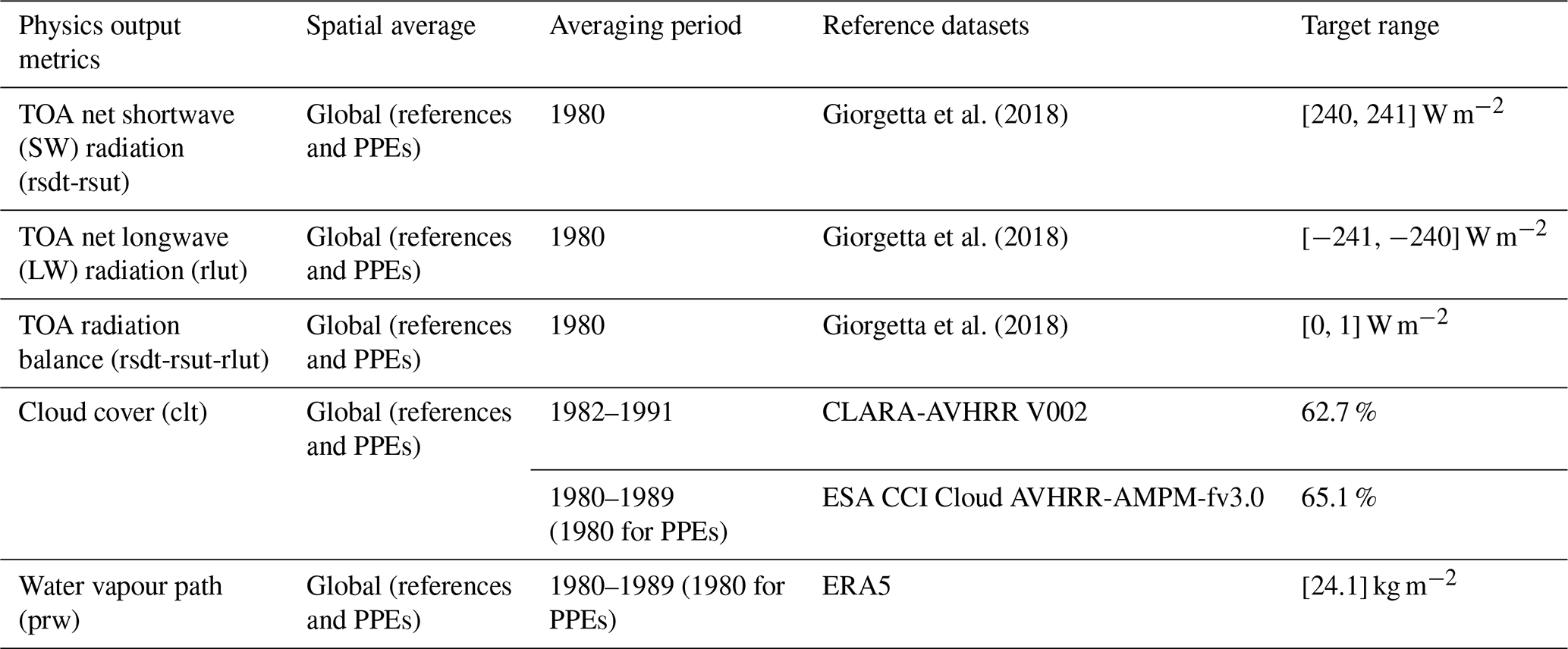
Table 1 reports the output metrics and the corresponding reference datasets and values that we focus on in this study, representing global radiative and cloud properties and referred to as the physics outputs. These physics output metrics are all global and multi-year averages. In particular, as shown in Table 1, we use the annual average over 1980 in our PPEs (apart from our last PPE, as discussed later) and compare it with the multi-year averages of the reference datasets.

Giorgetta et al. (2018)Giorgetta et al. (2018)Giorgetta et al. (2018)

Table 1 Physics outputs together with the respective observational datasets (CERES EBAF, NASA/LARC/SD/ASDC, 2019; ERA5, Dee et al., 2011; CLARA-AVHRR, Karlsson et al., 2020; and ESA CCI Cloud, Stengel et al., 2017) and target ranges used in this work. All the outputs in this table are globally averaged (for both the reference datasets and the ICON-A simulations we conduct). The averaging period used for both reference datasets and our simulations (PPEs) is reported in the third column. TOA stands for top of the atmosphere.

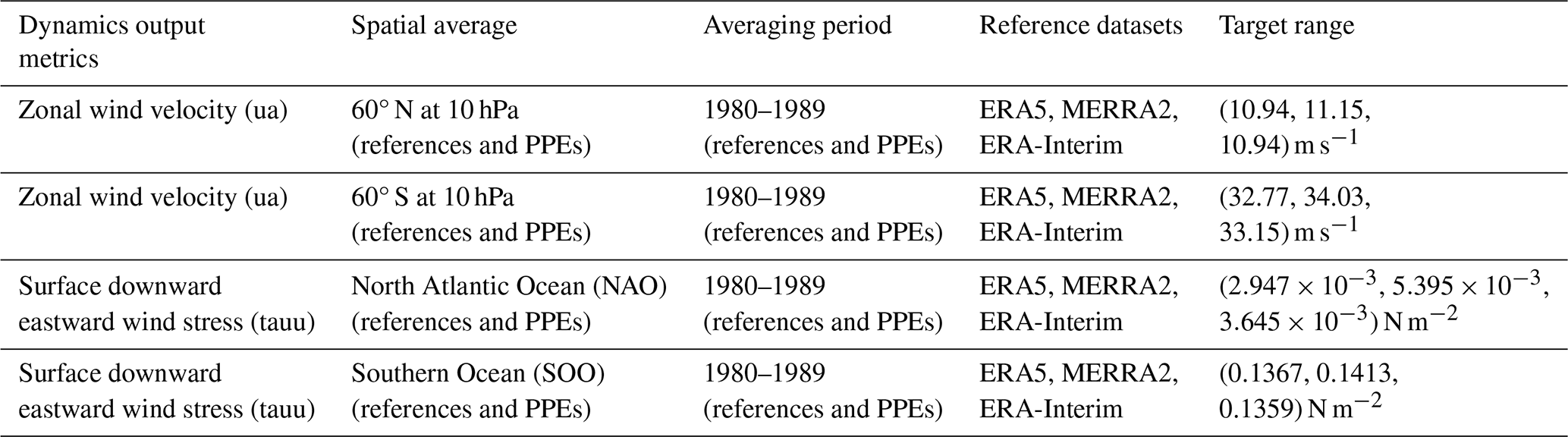
The output metrics related to atmospheric-circulation properties, the dynamics outputs, are given in Table 2. There, the zonal mean velocity at 60° N and S at 10 hPa serves as a proxy for the representation of high-latitude jets. This is a widely used target for evaluating simulations of the polar jets in models resolving the stratosphere (e.g. as seasonal means in Tripathi et al., 2014; Domeisen et al., 2020a, b; Rao et al., 2020; Baldwin et al., 2021). The surface downward eastward wind stress means over the North Atlantic Ocean and the Southern Ocean (defined in the AR6 database; Iturbide et al., 2020) are proxies for the forcing on the ocean surface. These dynamics output metrics are multi-year averages. In particular, as shown in Table 2, we use the average over the period 1980–1989 in our PPEs and compare it to the multi-year averages of the reference datasets reported in Table 2. We use different averaging periods for physics and dynamics outputs because of the different year-to-year variability and equilibration times of the associated variables. As substantiated in Sect. 3.3.1, the physics outputs have lower year-to-year variability compared to the dynamics ones, meaning that 1 simulated year is sufficient to obtain a representative value for the annual averages. Conversely, for dynamics metrics, the annual averages need to be estimated from multi-year simulations due to their larger variability and sensitivity to geographic patterns.

Table 2 Dynamics outputs together with respective observational datasets (ERA5, Hersbach et al., 2020) used in this work. The North Atlantic Ocean (NAO) region and the Southern Ocean (SOO) region are those defined in the AR6 database (Iturbide et al., 2020).

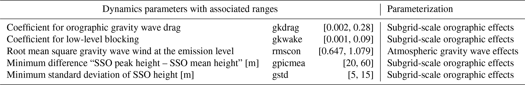
Following Giorgetta et al. (2018), the parameterizations we select for tuning the physics outputs are moist convection, vertical diffusion, cloud microphysics, and cloud cover. In Table 3, we report the parameters from these parameterizations (which we refer to as physics parameters) which we select for our tuning experiment. The parameterizations we select for tuning the dynamics outputs are the orographic and non-orographic gravity wave schemes. In Table 4, we report the parameters from these parameterizations (referred to as dynamics parameters) which we select for our tuning experiment.

Table 3 Tuning parameters related to physics parameterizations alongside the corresponding name in the ICON source code (second column from left), the range of values tested (third column from left), and the corresponding parameterization scheme they belong to (right column). The range of the parameters was inferred from the default value of the parameters given in the source code of ICON-A version 2.6.4.

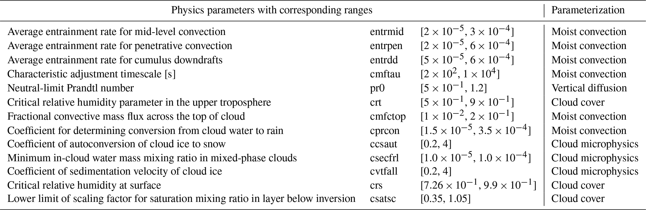
Table 4 Tuning parameters related to dynamics parameterizations alongside the corresponding name in the ICON source code (second column from left), the range of values tested (third column from left), and the corresponding parameterization scheme they belong to (right column). SSO stands for subgrid-scale orography.

2.3 Reference datasets

To tune ICON-A, we use reference values for the output metrics from Earth observations and reanalysis data. As in Giorgetta et al. (2018), the main goal here is to obtain a slightly positive global annual mean downward net radiation flux at the top of the atmosphere (TOA), between 0 and 1 W m⁻², based on a net shortwave flux and an outgoing longwave radiation close to observational estimates. For the two radiation fields (rsdt-rsut) and rlut (see Table 1 for definitions), the typical interval [240, 241 W m⁻²] is used as a reference value, as estimated in Giorgetta et al. (2018), following observational datasets (CERES EBAF Ed4.0, 2000–2016) and Kato et al. (2013) and Loeb et al. (2009). For cloud cover, we use CLARA-AVHRR (Karlsson et al., 2020) and ESA CCI CLOUD (Stengel et al., 2017), and for the water vapour path, we use ERA5 (Hersbach et al., 2020) (see Sect. A in the Appendix for time series of these observational datasets). For the dynamics outputs, we use ERA5, ERA-Interim (Dee et al., 2011), and MERRA2 (Gelaro et al., 2017). We refer the reader to Appendix A for the time series of some of the observational products used in this work.

2.4 ML-based tuning approach

Our ML-based tuning method is built on the history matching technique (Williamson et al., 2013, 2017) and follows a similar workflow to that in Couvreux et al. (2021); Hourdin et al. (2021, 2023). The goal is to find a region in the parameter space where the model outputs are compatible (within the observational uncertainty) with the observational data (observationally compatible). In performing this exploration, history matching aims to find a balance between exhaustively exploring or sampling the parameter space and minimizing the number of samples required for it. Since, in our case, each sample corresponds to a computationally expensive climate model simulation, we consider this method to be particularly well suited to our tuning task. In tuning ICON-A, we embed history matching in a sequential protocol, where, at each step, we add or remove tuning parameters based on the outcomes of the history matching iterations. We now start by outlining the steps of the history-matching-inspired method that constitutes the basis of our protocol (see also steps 1 to 4 in Fig. 1).

1. For a given set of tuning parameters 𝒫 with K elements, draw an initial Latin hypercube (LHC) sampling of size N. Using LHC sampling, all parameters are simultaneously changed, and the different samples fill the K-dimensional parameter space (within the allowed ranges specified in Tables 3 and 4) approximately uniformly. Typically, N is chosen as N≈10 K (Loeppky et al., 2009). Using these selected parameters, generate a PPE of ICON-A runs. The PPE consists of N members or runs, one for each sampled parameter configuration x_i (with i=1, …, N). For each run, we calculate all the output metrics described before. This results in sets of input–output training pairs ${\mathcal{T}}_Y=\mathit{\{}{\mathit{x}}_i,Y_{\mathrm{model}}({\mathit{x}}_i){\mathit{\}}}_{i=\mathrm{1},\mathrm{\dots },N}$, one set per output metric Y (e.g. annual average of global TOA radiation balance).

2. Fit an emulator to the generated PPE, i.e. to the training sets 𝒯_Y for all the output metrics Y of interest. For a given metric Y, the emulator evaluated based on a configuration of tuning parameters x returns Y_emul(x), the approximation of the true model output metric Y_model(x). Our choice for the model emulator is Gaussian process (GP) regression (Rasmussen and Williams, 2005). GPs are models typically used in Bayesian regression tasks and are very well suited to our case since (i) they have only a few parameters and hence require relatively little training data for fitting, and (ii) they, by construction, return the uncertainty associated with their prediction, which is measured by the variance Var(Y_emu(x)). This is a central quantity used in the steps below. Further details on the choice of the GP are given in Appendix B. In our implementation, we train one GP per model output.

3. Generate a large emulated metric ensemble of size M (typically ranging from 10⁵ to 10⁶; here, $M=\mathrm{3}\times {\mathrm{10}}^{\mathrm{5}}$) using the trained GP emulator. For each emulator run, calculate the implausibility measure ρ for each metric Y, with reference value Y⁰ (from observations or re-analysis data) as follows:

   $$\begin{array}{}\text{(1)}& \mathit{\rho }\left(Y_{\mathrm{emul}}\left(\mathit{x}\right),Y^{\mathrm{0}}\right)={\displaystyle \frac{|Y^{\mathrm{0}}-Y_{\mathrm{emul}}(\mathit{x}\left)\right|}{\sqrt{\mathrm{Var}\left(Y_{\mathrm{emul}}\left(\mathit{x}\right)\right)}}}.\end{array}$$

   The idea behind this definition is that a small distance $|Y^{\mathrm{0}}-Y_{\mathrm{emul}}(\mathit{x}\left)\right|$ or a large emulator variance $\sqrt{\mathrm{Var}\left(Y_{\mathrm{emul}}\right(\mathit{x}\left)\right)}$ (typically true when x is far from already sampled points) will lead to a small value of ρ, hence balancing exploitation with exploration of the parameter space. Note that, typically, a measure of the observational uncertainty Var(Y⁰) is included in the denominator of the implausibility measure and defines a tolerance for assessing the convergence of history matching. This is an important distinction between traditional history matching and our implementation, which we motivate in the next point. In our case, the observational uncertainty is accounted for in the evaluation of the tuned model configurations, where we assess whether the outputs of the parameter configurations sampled with our procedure (see next points) are within the spread of the observational datasets used as the reference. This is explained in Sect. 4.

4. Select N parameter configurations that satisfy the following constraints on the outputs (see Tables 1 and 2 for output definitions):

   • $\mathit{\rho }\left(Y_{\mathrm{emul}}\right(\mathit{x}),Y^{\mathrm{0}})<{\mathit{\rho }}_{\mathrm{1}}$ (for the three physics metrics of TOA shortwave radiation, TOA longwave radiation, and TOA net incoming radiation)

   • $\mathit{\rho }\left(Y_{\mathrm{emul}}\right(\mathit{x}),Y^{\mathrm{0}})<{\mathit{\rho }}_{\mathrm{2}}$ (for the two other physics metrics of cloud cover and liquid water path and the five dynamics metrics).

   The choice of a smaller threshold for the three radiation metrics is necessary in order to give a higher weight to the constraint on the balanced TOA radiation than on the other metrics. We use ρ₂=2ρ₁. The value of ρ₁ is automatically adjusted in order to select only N parameter sets out of the ensemble of size M. Given that we are interested in drawing parameter configurations that are representative of the space of plausible tuned parameters in only a few iterations, our choice of the implausibility measure, as in Eq. (1), provides stricter constraints on the selected parameters, with the observational means Y⁰ being the target values for the corresponding metrics.

5. Going back to step 1, generate a new PPE of size N with ICON-A for the parameter ensemble defined in the previous step, and repeat step 2 to step 4.

The iterations stop when one of the model configurations generated in the PPEs is compatible with observations or when a new set 𝒫 of tuning parameters is used. Compatibility with observations is defined based on a weighted distance of the model output metrics from their reference value, with a tolerance given by the corresponding observational uncertainty. The highest weight is given to the global TOA net radiation balance, our main tuning goal. In general, in the earlier iterations of history matching, not all the members of the next round are expected to be compatible with the observational references. The configurations that are found to be compatible with observations are considered to be representative of the space of plausible tuned parameters and are subsequently evaluated based on additional evaluation metrics to assess their quality as tuned configurations (see Sect. 4). The parameter set 𝒫 is changed when the spread of the PPE generated in the last history matching iteration is too far from the observational range. The new parameter set consists of new tuning parameters together with the most influential parameters from the previous 𝒫 for better steering the model outputs towards the observational references. The influence of the parameters on the model outputs is estimated by performing an emulator-based sensitivity analysis with Sobol indices, the details of which are provided in Sect. 3.2.2. This results in a sequential tuning approach, integrating history matching as its core component for constraining the parameters in the sets 𝒫 selected in the different phases. This is schematically shown in Fig. 1.

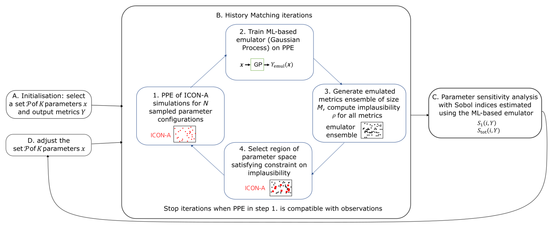
Figure 1 Schematic of the method used for the ML-based tuning of the physics parameters of ICON-A: history matching technique combined with a sensitivity analysis and a sequential parameter selection. The first set of tuning parameters is chosen (A), and history matching is employed to shrink the associated parameter space to an observationally compatible region (B). If the PPEs are far from observational references, a new parameter set is chosen with the help of sensitivity analysis (C). The new parameter set (D) is used for a new phase of the tuning experiment. When one or more of the model configurations generated in the last PPE are compatible with observations, the iterations of this tuning approach stop. The model configurations compatible with observations are then evaluated.

This sequential approach incorporating the previously explained history-matching-inspired method is used for the tuning of the physics outputs. The resulting model configuration serves then as basis for the next step, which is the simultaneous tuning of physics and dynamics parameters and metrics. Also, in this case, we use a sensitivity analysis to select which physics parameters to keep in this next tuning step. In this step for the tuning of physics and dynamics parameters and metrics, we follow the manual tuning approach of Giorgetta et al. (2018). We generate a PPE and select the best-performing model configurations, where our criterion for evaluating the model's performance keeps the highest priority on achieving a nearly balanced global annual net radiation flux at the top of the atmosphere (TOA). Separating the tuning of physics-only metrics from that also involving dynamics outputs allows us to use different durations of the ICON-A simulations for the two steps and to further reduce the computational costs. Specifically, as substantiated in Sect. 3.3.1, the physics outputs have lower year-to-year variability and shorter equilibration timescales compared to the dynamics outputs. This means that, for physics outputs, shorter simulations are needed for obtaining a representative value for the annually averaged variables used as metrics.

Finally, before moving on to the Results section, we offer a technical note on the construction and evaluation of the GP emulators: we implemented the GP emulator in Python using scikit-learn (https://doi.org/10.5281/zenodo.7711792, Grisel et al., 2024) and used the built-in routines to optimize the GP parameters at each iteration of the above procedure (see details in Appendix B). In this work, we measure the performance of the GP regression model via the R² value, which, for a given output Y, is defined as follows:

$$\begin{array}{}\text{(2)}& R^{\mathrm{2}}\left(Y\right)=\mathrm{1}-{\displaystyle \frac{\stackrel{\mathrm{‾}}{{\left(Y_{\mathrm{emul}}-Y_{\mathrm{model}}\right)}^{\mathrm{2}}}}{\mathrm{Var}\left(Y_{\mathrm{model}}\right)}},\end{array}$$

where $\stackrel{\mathrm{‾}}{(Y\mathrm{emul}-Y_{\mathrm{model}}{)}^{\mathrm{2}}}$ denotes the mean squared error of the emulator over a set of testing parameters, and Var(Y_model) denotes the variance of the true model output over the same test set.

3 Results

3.1 Summary of the generated PPEs

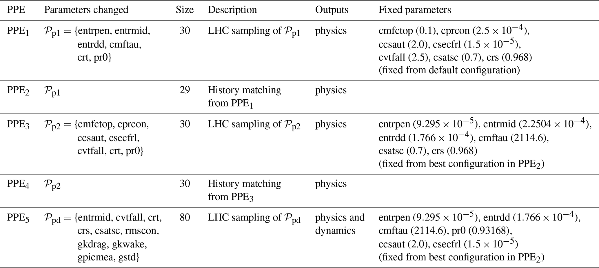
The PPEs generated in this work are summarized in Table 5. PPE₁ to PPE₄ are generated for the tuning of the physics output metrics from single-year ICON-A runs (1980) after a 1-year spin-up. PPE₁ is generated from an LHC sampling of size 30 based on the (physics) parameter set:

$$\begin{array}{}\text{(3)}& {\mathcal{P}}_{\mathrm{p}\mathrm{1}}=\mathit{\{}\mathrm{entrpen},\mathrm{entrmid},\mathrm{entrdd},\mathrm{cmftau},\mathrm{crt},\mathrm{pr}\mathrm{0}\mathit{\}},\end{array}$$

denoting the physics parameters used in Giorgetta et al. (2018). PPE₂ is produced by applying history matching to the results of PPE₁. After PPE₂, a new phase of our sequential approach starts: for PPE₃, we perform a new LHC sampling based on a modified parameter set,

$$\begin{array}{}\text{(4)}& {\mathcal{P}}_{\mathrm{p}\mathrm{2}}=\mathit{\{}\mathrm{cmfctop},\mathrm{cprcon},\mathrm{ccsaut},\mathrm{csecfrl},\mathrm{cvtfall},\mathrm{crt},\mathrm{pr}\mathrm{0}\mathit{\}},\end{array}$$

in order to increase the globally averaged cloud cover, which is consistently lower than the observational references in PPE₁ and PPE₂. The parameters in 𝒫_p2 were selected from those that, in the ICON-A manual tuning history (unpublished), were deemed to be most influential for cloud cover. Our criterion to decide which parameters to keep from 𝒫_p1 to 𝒫_p2 follows from the sensitivity analysis based on Sobol indices, which we present later in Sect. 3.2.2. Specifically, the parameters crt and pr0, associated with higher first and total Sobol indices for the cloud and water vapour metrics, have been kept from 𝒫_p1 to 𝒫_p2. For generating PPE₃ and PPE₄, the values of the parameters in 𝒫_p1 that are not present in 𝒫_p2 are fixed at their best value from PPE₂ (see the right column of Table 5 and the magenta star in Figs. 2 and 3). The set 𝒫_p2 is used to generate PPE₃, consisting of 30 samples sampled with LHC sampling. PPE₄ is produced by applying history matching to the results of PPE₃. The sizes of the PPEs are chosen to be smaller than the typical value of 10 times the number of parameters (six parameters in 𝒫_p1 and seven parameters in 𝒫_p2) (Loeppky et al., 2009). This size allows a lower computational cost while being large enough to train an emulator that allows convergence of the PPEs towards reference observations, as explained in Sect. 3.2.1.

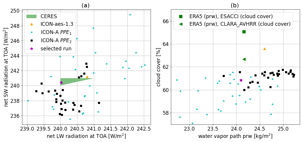
Figure 2 Physics output variables for PPE₁ (blue stars) and PPE₂ (black squares) compared to ICON-aes-1.3 (orange triangle) and observational datasets (green). Signs of convergence of history matching are visible already after one iteration (the distribution of the members of PPE₂ is slightly shifted towards higher cloud cover values and is narrower). The magenta star marks the best-performing configuration from PPE₂ (see right column of Table 5) used in the generation of the subsequent PPEs.

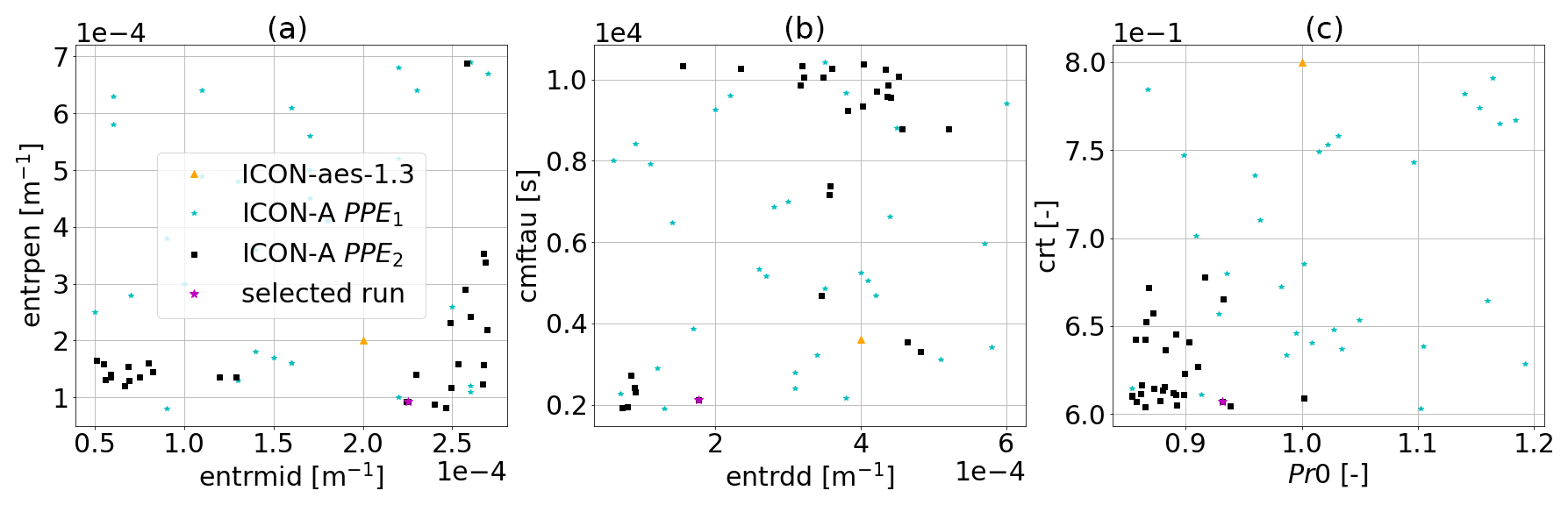
Figure 3 Sampled parameter values for PPE₁ (blue stars) and PPE₂ (black squares) compared to ICON-aes-1.3 (orange triangle). For each panel, two parameters are plotted on the two axes (see Table 3). Signs of convergence of history matching are visible already after one iteration (in the distribution of the members of PPE₂ being slightly shifted and narrower). The magenta star marks the best-performing configuration from PPE₂ (see also right column of Table 5 for values) used in the generation of the subsequent PPEs.

In PPE₅, we then also address the tuning of dynamics outputs by varying physics and dynamics parameters simultaneously in the parameter set,

$$\begin{array}{}\text{(5)}& \begin{array}{rl}{\mathcal{P}}_{\mathrm{pd}}=& \left\{\mathrm{entrmid},\mathrm{cvtfall},\mathrm{crt},\mathrm{crs},\mathrm{csatsc},\mathrm{rmscon},\mathrm{gkdrag},\right.\\ & \left.\mathrm{gkwake},\mathrm{gpicmea},\mathrm{gstd}\right\},\end{array}\end{array}$$

and keeping the other parameters fixed at their best values in PPE₂ (see the right column of Table 5 and the magenta star in Figs. 2 and 3). Also, for 𝒫_pd, we follow the same strategy and keep the parameters with the highest influence on the radiation and water metrics, as can be seen from the Sobol analysis in Sect. 3.2.2, with the addition of crs and csatsc after further advice from ICON experts. The parameters rmscon, gkdrag, and gkwake are the same dynamics parameters used in Giorgetta et al. (2018), and we added gpicmea and gstd following advice from ICON expert knowledge. PPE₅ consists of 10-year ICON-A simulations from 1980 to 1989 (after a 1-year spin-up).

Table 5 Summary of perturbed parameter ensembles (PPEs) generated in this work. The PPEs have been sequentially generated from 1 to 5. PPE₃ is obtained from an LHC sampling of parameter set 𝒫_p2, where the parameters in 𝒫_p1 and not included in 𝒫_p2 are kept fixed at their best values from PPE₂ (listed in the right column), which are then used further in PPE₄ and PPE₅.

3.2 ML-based tuning of physics outputs with history matching

In this section, we present the results of the tuning of the physics parameters. We start by considering PPE₁ and PPE₂. As explained before, PPE₂ is generated by applying history matching after having trained a GP emulator on the outputs of PPE₁. The constructed GP emulator, in this case, has a good predictive performance (measured by an average R² score of 0.81, as discussed in more detail in Sect. 3.2.1 below) and can therefore accurately guide the parameter choices for PPE₂. Thanks to this, the application of only one iteration of history matching to PPE₁ is already sufficient to generate configurations in PPE₂ that achieve a balanced TOA radiation. This is demonstrated in Fig. 2a, which shows the net shortwave (SW) versus the net longwave (LW) TOA radiation for PPE₁ and PPE₂. There, we can clearly see that, after history matching based on PPE₁, PPE₂ can achieve configurations that match or get close to the observational ranges denoted by the green triangle (and to ICON-aes-1.3). The convergence of the output metrics towards their reference values can also be observed in Fig. 2b for the other two physics output metrics (global cloud cover versus water vapour path) for PPE₁ and PPE₂. There, the distribution of the PPE₂ outputs converges towards the observational references (green markers). The convergence of history matching towards the observational references can also be seen in the distribution of the sampled parameters for the two PPEs (Fig. 3). However, Fig. 2b shows that global cloud cover still remains lower than the observational data (by approximately 1 % compared to CLARA-AVHRR and 3 % compared to ESA CCI Cloud) despite PPE₂ yielding a slightly higher cloud cover (closer to the observed range) than PPE₁. In Fig. 2, the magenta star marks the selected best-performing model configuration in PPE₂. Following Giorgetta et al. (2018), our criterion for evaluating the model performance prioritizes the global radiation metrics, particularly the net TOA radiation budget, over cloud cover and water vapour path. The selected run is the only one falling within the observational range for both radiation metrics (green triangle in Fig. 2a).

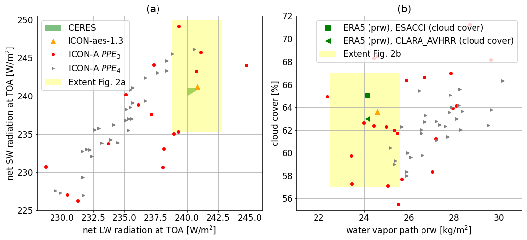
Figure 4 Physics output variables for PPE₃ (red circles) and PPE₄ (grey triangles) compared to ICON-aes-1.3 (orange triangle) and observational datasets. Signs of convergence of the outputs to their observational values can also be seen here (in the distribution of the members of PPE₄ being slightly shifted and narrower).

ICON-aes-1.3 exhibits a higher value of global cloud cover (orange triangle in Fig. 2b) than our PPE₁ and PPE₂. The resolution of ICON-aes-1.3 (approximately 160 km) is coarser than that of PPE₁ and PPE₂ (approximately 80 km). The authors of Giorgetta et al. (2018) have investigated the six tuning parameters used in 𝒫_p1. Here, with these six parameters, we are not able to reach a similar performance for the cloud cover metric. This supports the fact that one should repeat the tuning process when the model resolution is changed (Crueger et al., 2018). Moreover, in addition to the parameters in 𝒫_p1, the authors of Giorgetta et al. (2018) explored other tuning parameters, and these results were not published due to a negligible influence on their tuning process (as explained in their Sect. 5). In the next generation of PPEs (the second phase of our sequential approach), we investigate the impact of some of these parameters. Therefore, the parameter set 𝒫_p2 contains parameters that potentially have a stronger effect on cloud cover at the present resolution.

Parameter set 𝒫_p2 is used to generate PPE₃ with LHC sampling. A GP emulator is then trained on the outputs of PPE₃. The constructed GP emulator in this case also has a good predictive performance (measured by an average R² score of 0.75, as discussed in more detail in Sect. 3.2.1 below), and we therefore use it for performing history matching and generating PPE₄. Also, in this case, history matching is shrinking the space of promising parameter configurations and the related output distribution. This can be seen in Fig. 4, where we show the distribution of the radiation metrics (in Fig. 4a) and that of global cloud cover versus water vapour path (in Fig. 4b) for both PPE₃ and PPE₄ (we refer the reader to Appendix C for plots of the related parameter distributions). While the new parameter set 𝒫_p2 allows us to reach a global cloud cover consistent with observations, we also see that the spread of the PPE outputs is more than doubled compared to that of the previous PPEs (see yellow-shaded rectangles in Fig. 4, showing the extent of Fig. 2). This increased spread also potentially increases the number of history matching iterations converging towards the observational references. Given the high computational costs of generating these PPEs, we use the best-performing model configuration sampled so far, which belongs to PPE₂.

3.2.1 Performance of the GP emulator

We now analyse the performance of the GP emulator for the physics outputs considered. We refer the reader to Appendix B for details on Gaussian processes and the choice of the underlying hyperparameters. In Table 6, we show the average performance (R² score) of the GP emulators trained on the PPEs used for the tuning of the physics parameters (corresponding to PPE₁, PPE₂, PPE₃, and PPE₄). The value reported in Table 6 is the average R² over all five of the physics output metrics (defined in Table 1) and is computed using a 5-fold cross-validation (https://doi.org/10.5281/zenodo.7711792, Grisel et al., 2024). From these values, we conclude that the constructed emulators are indeed able to approximate the ICON-A physics outputs, which is also reflected in the fact that history matching already shows signs of convergence after the first iteration, as shown in the previous section. The number of PPE samples required for the GP regression to achieve the reported R² score is shown in Fig. 5.

Table 6 Performance of the GP emulator based on PPE₁ to PPE₄. The R² value reported here is the average R² of the emulators for all physics variables (see Table 1). For each emulator, the R² is calculated via 5-fold cross-validation on the training set (PPE points).

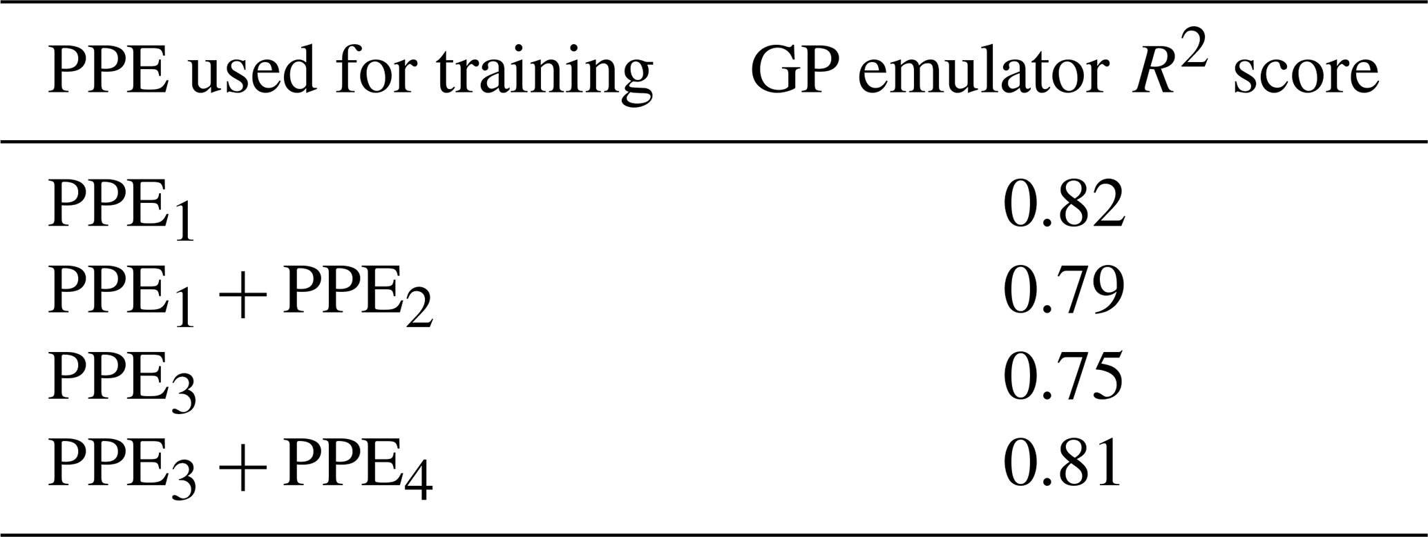
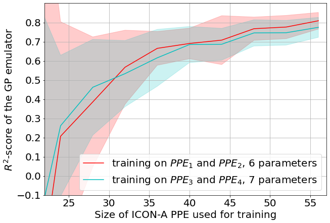
Figure 5 Average R² score of the physics output emulators as a function of the size N of the PPE used for training. For each N tested, 50 random samples of size N were drawn from the entire set of ICON PPEs of size 60. The R² score is calculated for each size N sample, and the mean (solid lines) and standard deviation (shaded areas) are estimated from these scores of the 50 samples. The red curve shows the R² for emulators trained on PPE₁ and PPE₂, and the blue curve shows the R² for emulators trained on PPE₃ and PPE₄.

3.2.2 Sensitivity analysis for the physics parameters and outputs

In this section, we show the sensitivity analysis for the physics parameters and outputs, supporting our selection of parameters in the subsequent steps of our sequential approach as presented in Sect. 3.1. The analysis presented here is based on the calculation of Sobol indices, which, in turn, are calculated using the emulator constructed in the previous section. Generally speaking, Sobol indices quantify the impact of one specific feature (tuning parameter, in our case) on the overall variance of the model output (the output metrics, in our case). Specifically, we focus on the first-order Sobol index and on the total Sobol index. Given an emulator Y_emul for metric Y, the first-order and total Sobol indices for the ith parameter x_i are defined as follows (Saltelli et al., 2010):

$$\begin{array}{}\text{(6)}& {\displaystyle }& {\displaystyle }{S}_{\mathrm{1},(i,Y)}={\displaystyle \frac{\mathrm{1}}{{\mathrm{Var}}_{\mathit{x}}\left(Y_{\mathrm{emul}}\right)}}{\mathrm{Var}}_{x_i}\left({\mathbb{E}}_{{\mathit{x}}_{\sim i}}\left(Y_{\mathrm{emul}}|x_i\right)\right),\text{(7)}& {\displaystyle }& {\displaystyle }{S}_{\mathrm{tot},(i,Y)}={\displaystyle \frac{\mathrm{1}}{{\mathrm{Var}}_{\mathit{x}}\left(Y_{\mathrm{emul}}\right)}}{\mathbb{E}}_{{\mathit{x}}_{\sim i}}\left({\mathrm{Var}}_{x_i}\left(Y_{\mathrm{emul}}|{\mathit{x}}_{\sim i}\right)\right),\end{array}$$

where Var_x(Y_emul) denotes the sample variance of the emulator over the distribution of all parameters x, ${\mathrm{Var}}_{x_i}(\cdot )$ denotes the sample variance of the emulator over the distribution of parameter x_i, ${\mathbb{E}}_{{\mathit{x}}_{\sim i}}$ denotes the expected value over all parameters but x_i, and Y_emul|x_i denotes the emulator function with input parameter x_i kept fixed. The first-order Sobol index $S_{\mathrm{1},(i,Y)}$ corresponds to the effect of varying x_i alone, averaged over all other input (parameter) variations, while $S_{\mathrm{tot},(i,Y)}$ measures the total effect of varying x_i, which includes the variance coming from interactions of x_i with other parameters. In Fig. 6, we show the $S_{\mathrm{1},(i,Y)}$ (on the x axis) and $S_{\mathrm{tot},(i,Y)}$ (on the y axis) for the physics parameters and outputs. We use the GP emulator trained on PPE₁ for Fig. 6a–e and the one trained on PPE₃ for Fig. 6f–j. The higher the values of the first-order and total Sobol indices for a parameter and its corresponding output, the higher the influence of that parameter on that output. Looking at Fig. 6d and e, we see that the two most influential parameters in 𝒫_p1 in relation to cloud cover and water vapour metrics are crt and pr0, which are the ones we keep among the tuning parameters in 𝒫_p2. In Fig. 6f–j, obtained from the emulator trained on PPE₃, we see that cvtfall has, overall, a large effect on all physics metrics and the largest effect on cloud cover, while crt has the largest effect on the TOA net radiative budget; we therefore decide to keep these tuning parameters in 𝒫_pd for PPE₅.

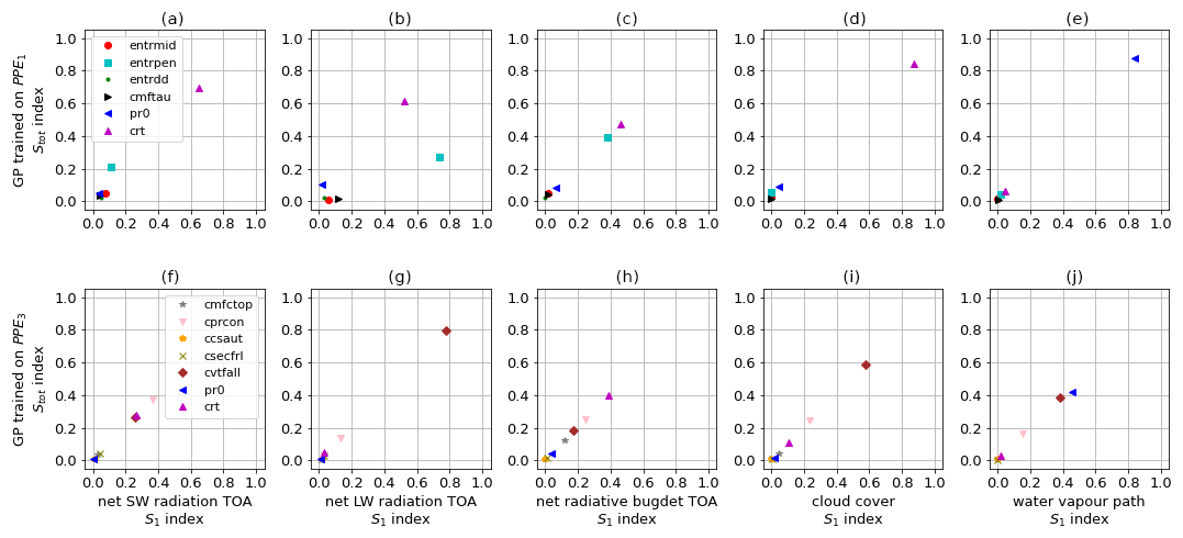
Figure 6 First-order Sobol index S₁ (x axis) and total Sobol index S_tot (y axis) for the physics parameters (in legend) and outputs: net SW radiation at TOA (panels a and f), net LW radiation at TOA (panels b and g), net radiative budget at TOA (panels c and h), cloud cover (panels d and i), and water vapour path (panels e and j). We use the GP trained on PPE₁ for panels (a)–(e) and that trained on PPE₃ for panels (f)–(j). To calculate the Sobol indices, the sampling method of Saltelli et al. (2010) was used, with 70 000 samples, allowing for a converged value of the indices.

3.2.3 Visualization of the parameter-to-output maps

The previously trained emulator can also be used for the visualization of the parameter-to-output dependencies. These visualizations complement the sensitivity analysis presented in the previous section and further helped us in the selection of the tuning parameters to be kept across the phases of our sequential tuning approach. Generally, such visualizations are very useful for informing the user of the effect of a parameter on the outputs: they can help in selecting the most influential parameters and the corresponding plausible ranges, potentially reducing the computational costs of tuning exercises.

Here, we construct these parameter-to-output maps, similarly to what has been done by Mauritsen et al. (2012), with the important difference being that the use of GP emulators in our case allows for a more extensive or denser exploration of the selected parameter space. We exemplify such visualizations in Fig. 7, constructed from GP emulators for physics outputs trained on PPE₁ and PPE₂ in the first two lines (Fig. 7a–h) and on PPE₃ and PPE₄ in the last two lines (Fig. 7i–p). The parameters that are not being changed are kept fixed at their best-performing value from PPE₂ (marked with the magenta star in Figs. 2 and 3 – although we emphasize that, with the trained emulators, one can very quickly generate new maps for different parameters). The red-shaded areas in each plot denote the allowed output ranges from the observational data. When the parameters from 𝒫_p1 are varied, the value of global cloud cover (second row of Fig. 7) remains below the lower bound given by the observational data (at 62.7 %), which is consistent with our observations in Fig. 2. This is the reason why we selected an increased parameter set 𝒫_p2 for the next PPEs, which, indeed, had a higher influence on the global cloud cover (fourth row of Fig. 7). We refer the reader to Appendix E for the parameter-to-output map constructed from PPE₁ and PPE₂, showing the effect of the six parameters in 𝒫_p1 on all physics metrics (Fig. E1). Likewise, the parameter-to-output map constructed from PPE₃ and PPE₄, showing the effect of all parameters in 𝒫_p2, is shown in Fig. E1.

Together with Sect. 3.2.2, these maps allow us to identify which parameters are likely to be the most influential for our physics tuning metrics. The parameters that we identified as most influential for the physics output metrics are the critical relative humidity in the upper troposphere (crt) and the coefficient conversion from cloud water to rain (cprcon), influencing the radiation metrics and global cloud cover, together with the coefficient of sedimentation velocity of cloud ice (cvtfall). These parameters have a strong linear influence (crt in Fig. 7d and h) and non-linear influence (cprcon and cvtfall in Fig. 7j and n and l and p, respectively) on the physics metrics. Note that parameters governing cloud microphysical processes (e.g. fall velocities such as cvtfall) were identified as tuning parameters widely shared among climate models in the synthesis paper of Hourdin et al. (2017) (see Table ES4 therein).

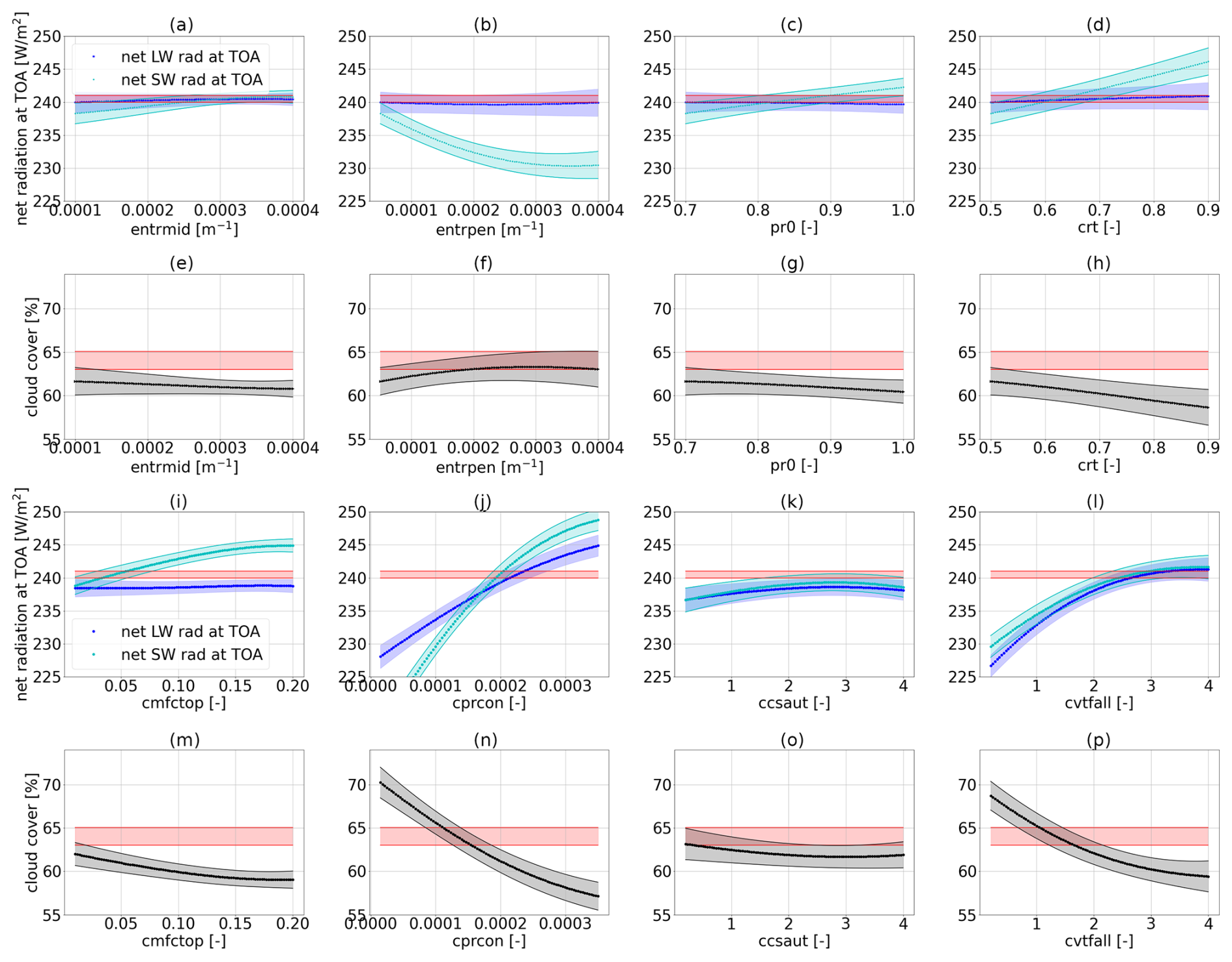
Figure 7 Parameter-to-output maps predicted with GP emulators trained on PPE₁ and PPE₂ (a)–(h) and GP emulators trained on PPE₃ and PPE₄ (i)–(p). In the first and third rows (a–d and i–l) the net SW and LW radiation at the TOA are shown. In the second and fourth rows (e–h and m–p) the global cloud cover is shown. Panels (a) and (e) show the effect of entrmid, (b) and (f) show that of entrpen, (c) and (g) show that of pr0, (d) and (h) show that of crt, (i) and (m) show that of cmfctop, (j) and (n) show that of cprcon, (k) and (o) show that of ccsaut, and (l) and (p) show that of cvtfall.

3.3 Tuning of the dynamics outputs

We now discuss the simultaneous tuning of the physics and dynamics outputs. Due to the expected large variability in dynamics outputs (see Sect. 3.3.1), which can potentially hinder the training of regression models, we expect history matching to require a large number of iterations and costly ICON simulations. Therefore, we adopt a similar approach to Giorgetta et al. (2018) in that we generate a PPE (PPE₅) and select the best-performing model configurations. Also, in this case, our criterion for evaluating the model performance gives a higher importance to the global radiation metrics, which are our primary tuning goals, and puts less stringent requirements on the other tuning metrics.

The ML-based tuning of the physics output metrics discussed in the previous section serves as a basis for the second tuning step addressing the dynamics outputs. PPE₅ is generated by simultaneously varying the parameters in the set 𝒫_pd (with LHC sampling) while keeping the other parameters fixed to their best configuration obtained with history matching from PPE₂ (see Table 5 and the magenta star in Figs. 2 and 3). The physics parameters in 𝒫_pd are selected based on a sensitivity analysis with Sobol indices, as explained in Sect. 3.2.2. The choice of the dynamics parameters follows Giorgetta et al. (2018), with gkdrag and gkwake being chosen for tuning the zonal wind stresses on the ocean surface and rmscon affecting the zonal mean winds. In Fig. 8, we show the physics (Fig. 6a and b) and the dynamics (Fig. 6c and d) outputs from PPE₅ and highlight the two model configurations (the cyan and the red dots) which achieve the best model performance within PPE₅. The selected configurations are those closest to the observational range in Fig. 8a, given that achieving a balanced TOA radiation has higher importance in our tuning experiment (Giorgetta et al., 2018). The values of the parameters for these two selected simulations are given in Table 7. These also achieve results comparable with the tuned ICON-aes-1.3, with the TOA radiation balance being within the interval [0, 1] W m⁻², where the TOA longwave and shortwave radiation metrics are within 1 W m⁻² from the observational range. Also, for the other two physics output metrics, the performance of the two selected configurations is comparable to ICON-aes-1.3 as they show less than 1 % difference in global cloud cover compared to the observational range and less than 0.5 kg m⁻² difference in the water vapour path. The differences with respect to reference data and ICON-aes-1.3 become more apparent when looking at the dynamics metrics. In Fig. 8c and d, it can indeed be seen that the values of these metrics from the reference dataset are not covered by the generated PPE. For most of the metrics, the differences in terms of the selected configurations from the reference dataset remain comparable to those of ICON-aes-1.3, except for the mean zonal wind stress over the Southern Ocean (tauu SOO – see Fig. 8c), where the difference increased from roughly 0.005 N m⁻² to roughly 0.02 N m⁻². The values of the parameters for these two selected runs are given in Table 7. Given the different settings used in the manual tuning for ICON-aes-1.3 (160 km instead of the 80 km resolution used here, along with the different time steps used), the differences in the optimal model configurations are not surprising. For instance, the model resolution strongly affects the parameters describing the unresolved orography and, thus, the values of the corresponding parameters (Giorgetta et al., 2018).

In the next section, we analyse the variability of the dynamics outputs, and we identify a possible explanation for the difficulty in matching them in our tuning. Afterwards, in Sect. 4, we evaluate the results from PPE₅ regarding model outputs not targeted during the tuning experiment for a better assessment of the results and a better comparison with the previously tuned ICON-aes-1.3.

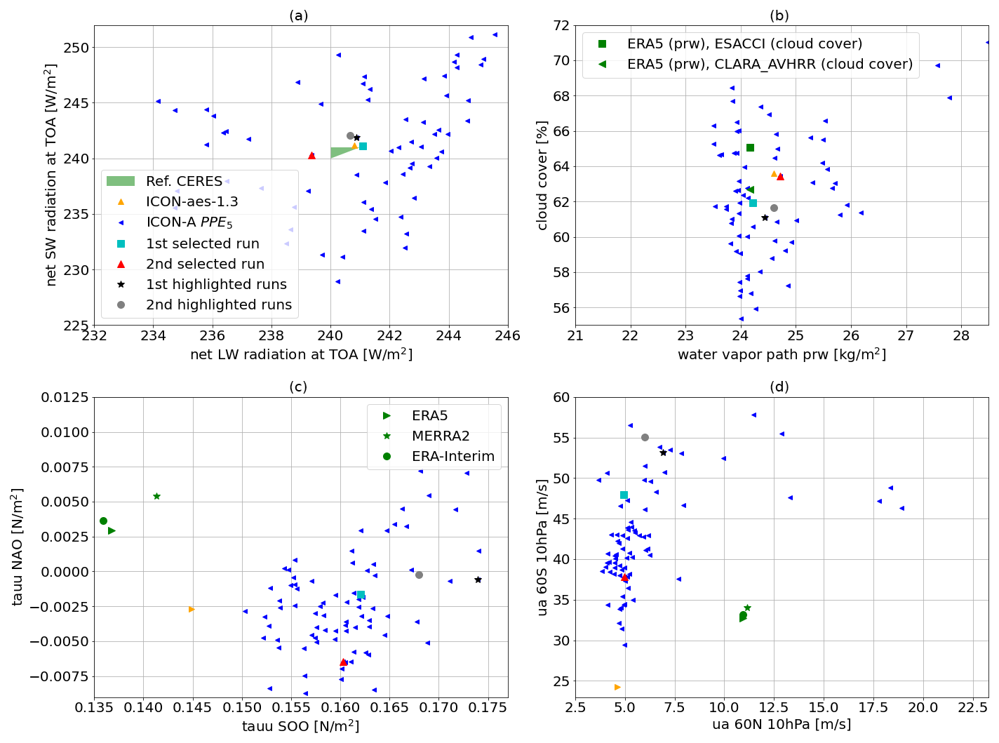
Figure 8 Physics (a, b) and dynamics (c, d) output variables for PPE₅ (blue triangles) compared to ICON-aes-1.3 (orange triangle) and observational datasets. Two selected PPE members corresponding to the best-performing configurations are highlighted (cyan square and red triangle). For comparison, two other runs are also highlighted (black circles).

Giorgetta et al. (2018)

Table 7 Values of the parameters for the two members of PPE₅ yielding the best output metrics, shown as cyan square and red triangle in Fig. 8. For comparison, the values of the parameters tuned by Giorgetta et al. (2018) are given as well.

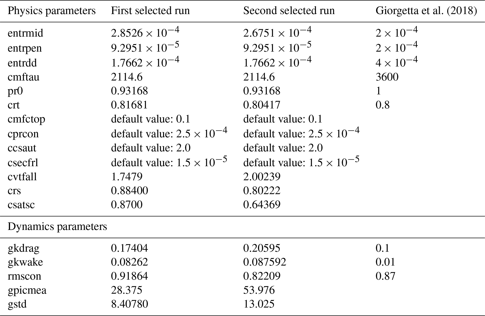
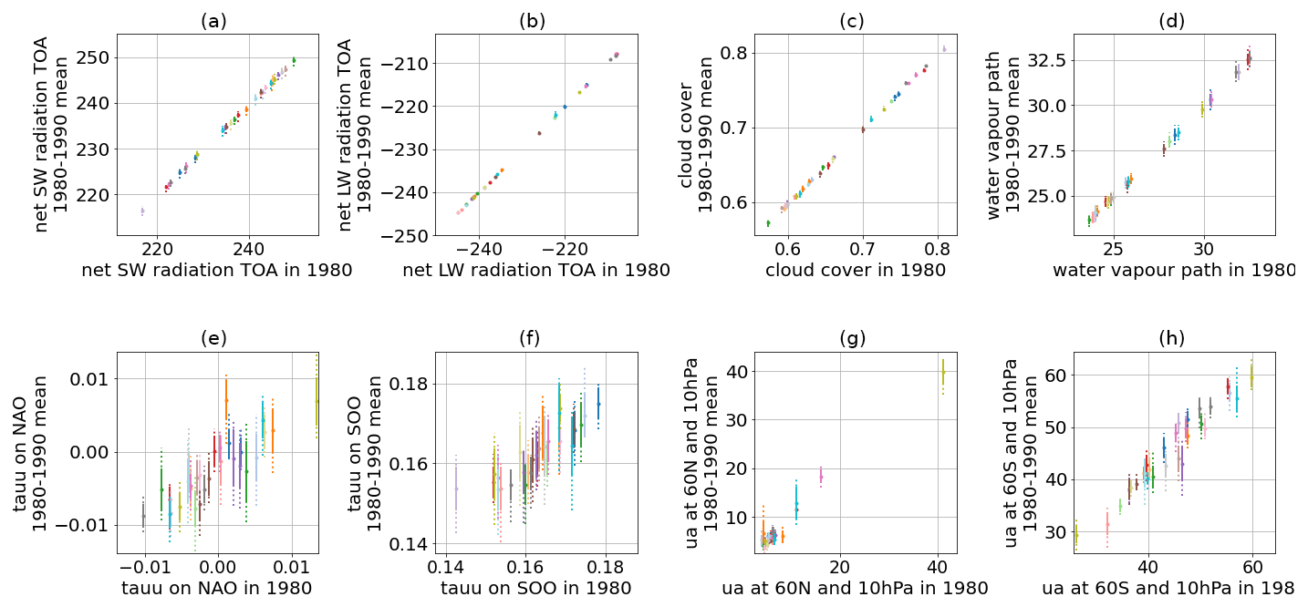
Figure 9 The 10-year mean (1980–1989, y axis) against the mean of 1 particular year (here 1980, x axis) for the physics (top row, panels a–d) and dynamics (bottom row, panels e–h) output variables for 30 runs of PPE₅, represented by different colours. For each data point, the dotted vertical line shows the spread of the annual mean across the 10 years (maximum and minimum values), and the solid vertical line denotes 1 standard deviation, calculated based on the 1980–1989 period.

3.3.1 Analysis of output variability

We now use PPE₅ to analyse the internal variability of the investigated output metrics and compare them to the parameters' effects. The year-to-year variability of the output metrics is shown in Fig. 9, where we plot the long- vs. short-time averages of the considered outputs for 30 runs of PPE₅. Additional data complementing the information of Fig. 9 can be found in Appendix D. In Fig. 9, it can be clearly seen that the dynamics outputs (panels in the lower row) have a larger variability across years compared to the physics ones (upper row), which is apparent from the larger spread around the diagonal (no spread would signify no variance) and the larger error bar (which represents the standard deviation over the yearly averages). In each panel, we also report the ratio between the mean spread across years S_yrs and the PPE spread S_PPE, which, for each output metric Y, are defined as follows:

$$\begin{array}{}\text{(8)}& {\displaystyle }& {\displaystyle }{S}_{\mathrm{yrs}}=\sqrt{{\displaystyle \frac{\mathrm{1}}{n}}\sum _{i=\mathrm{1}}^n{\mathrm{Var}}_{\mathrm{years},i}\left(Y\right)},\text{(9)}& {\displaystyle }& {\displaystyle }{S}_{\mathrm{PPE}}=\sqrt{{\displaystyle \frac{\mathrm{1}}{n}}\sum _{i=\mathrm{1}}^n{\left(Y_i-\stackrel{\mathrm{‾}}{Y}\right)}^{\mathrm{2}}},\end{array}$$

where n denotes the size of the PPE, Var_years,i(Y) denotes the variance of output Y over the simulated years for the ith PPE member, Y_i denotes the 10-year mean of output Y for the ith PPE member, and $\stackrel{\mathrm{‾}}{Y}$ denotes the average of Y_i over all PPE members. The ratio $S_{\mathrm{years}}/S_{\mathrm{PPE}}$ gives a quantitative measure of the comparison between the yearly output variability and the effects of changing parameters in the PPE. It is clear that, for the dynamics outputs, especially the zonal wind stresses on the ocean surface, this ratio is almost 1 order of magnitude larger than for the physics ones.

An additional source of uncertainty in the dynamics output metrics is their restricted geographical location, which exposes them to biases in spatial patterns. The low variability in the physics variables, which are global means, is consistent with the common observation that, already, simulations as short as 1 year can give good tuning results, though using more years, for instance, a full decade, as used in Giorgetta et al. (2018), has the benefit of including a larger variation of prescribed boundary conditions, for example, El Niño, La Niña, or neutral years.

The analysis shown in Fig. 9 shows that, for dynamics outputs, the internal variability is almost of the same order of magnitude as the PPE variance and can therefore partly hide the effects of changing parameters, as discussed above.

4 Evaluation of the selected runs

Now, we test our selected model configurations on different variables that were not targeted during the tuning. We call these “evaluation metrics”. Specifically, we assess whether the outputs of our selected parameter configurations are also compatible with the evaluation metrics, i.e. within the spread of the reanalysis and observational datasets used as a reference. This evaluation step allows us to check whether the tuning process has induced significant biases in metrics not targeted during the tuning (i.e. over-tuning of the target metrics). The evaluation metrics that we inspect are the global multi-annual averages (from 1980 to 1989) of the surface temperature (ts), the total precipitation (pr), the pressure at sea level (psl), the vertically integrated cloud ice (clivi), and the vertically integrated cloud condensed-water content (clwvi). The results of this evaluation step are shown in Fig. 10. For most of the computed evaluation metrics, our selected model configurations are within the observational range given by the spread of the reanalysis and observational datasets used as a reference (green symbols and lines in Fig. 10), thus indicating that our tuning experiment had a beneficial effect on the evaluation metrics that were not targeted by the tuning. This is the case for the two selected runs and the two highlighted runs from the ICON-A PPE₅. These selected model configurations show a slight positive bias of < 0.1 °C in terms of the global average of the surface temperature compared to the reference values. We conclude that our tuning experiment successfully produced configurations largely comparable to ICON-aes-1.3, while it did not show substantial improvement over the manually tuned version, which is difficult to improve upon. We discuss the limitations of our approach and propose potential improvements in the next section.

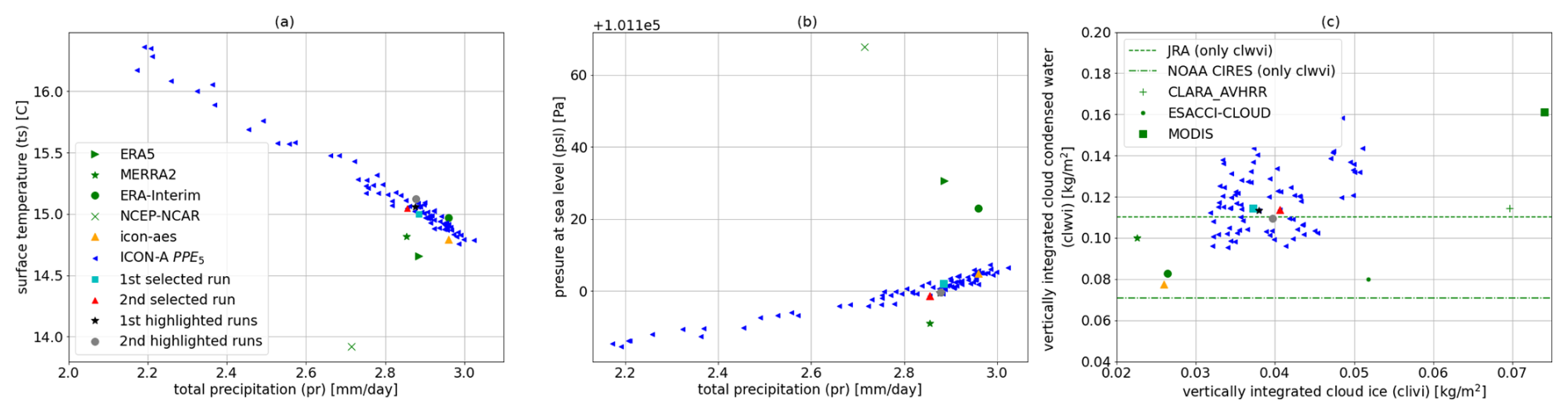
Figure 10 Five evaluation metrics averaged for the 1980–1989 (included) period for the PPE₅ (blue, cyan, red, black, grey), ICON-aes-1.3 (orange triangle), and reanalysis datasets and observational datasets (green). For the datasets starting after 1980, the time period considered is the earliest available 10 years: for CLARA (AVHRR) and ESA CCI Cloud (AVHRR-fv3.0), it is 1982–1991, and for MODIS, it is 2002–2011.

5 Discussion and conclusions

In this work, we develop an ML-based tuning approach and apply it to the atmospheric component of the ICON climate model (ICON-A). Our approach is inspired by history matching (Williamson et al., 2013, 2017), which balances an extensive exploration of the tuning parameter space with the need to minimize the number of required ICON-A model simulations. This exploration is aided by building and using emulators – here, Gaussian processes (GPs) – for each of the considered output metrics. The emulator approximates the climate model simulation outputs for arbitrary values of the tuning parameters and can be used to create large emulated metric ensembles at a much cheaper computational cost. We integrate a history-matching-inspired method in a sequential approach, where, in each phase, different parameter sets are sequentially constrained. We first apply our approach to the tuning of physics output metrics (globally averaged radiation and cloud properties), and, in a second step, we also tune for dynamics output metrics (related to geographically specific atmospheric-circulation properties) using a PPE consisting of 80 10-year ICON-A runs. The ML-based tuning of physics parameterizations, with just one iteration and a total of 60 model simulations, is already sufficient to achieve a model configuration yielding a global TOA net radiation budget in the range of [0, 1] W m⁻², global radiation metrics and water vapour paths consistent with the reference observations, and a globally averaged cloud cover differing by only 2 % with respect to the observations. Note that these results, particularly the number of iterations necessary to converge with the observational range, generally depend on the specific setup. Furthermore, we remark that our approach presents some differences compared to traditional history matching implementations. While it allowed us to draw some configurations with outputs compatible with observations for some metrics, a thorough characterization of the space of plausible parameters (the not-ruled-out-yet space; Williamson et al., 2013) is beyond the scope of our work and would require several iterations of standard history matching.

In the simultaneous PPE-based tuning of physics and dynamics parameterizations, we achieve a TOA radiation balance within the interval [0, 1] W m⁻², with TOA longwave and shortwave radiation metrics that are within 1 W m⁻² of the targeted range, but we are not able to reduce the biases in the dynamics output metrics with respect to the previously manually tuned ICON-aes-1.3. The PPE for this tuning step allows us to perform an analysis of the physics and dynamics output variability and a comparison with the parameters' effects. This analysis reveals a larger year-to-year variability in the dynamics compared to the physics output metrics. This, combined with the sensitivity of the dynamics metrics to geographic pattern, highlights potential limitations that emulator-based approaches may face when tuning for these dynamics metrics. This suggests, at the same time, that metrics averaged over broader spatial regions may suffer less from these issues and be more amenable to emulator-based approaches, although too much averaging in space would make the tuning target less characteristic. For the case of the dynamics variables which are proxies for polar stratospheric vortices (zonal mean zonal wind, averaged at 60° N and 60° S at 10 hPa over 10 years), a possible way to reduce the noise would be to increase the simulation duration and to average the field over only winter or summer months. A further evaluation of the selected model configurations based on metrics that were not targeted during tuning suggests that our approach does not cause over-tuning in relation to the tuning targets and, for our use case, results in a model configuration that can be considered to show similar performance compared to the previously tuned ICON-aes-1.3.

Our sequential approach, in which, at each phase, only a small subset of parameters is varied, allows us to keep the costs of the PPEs relatively low (with 30 members, we could reach good emulator accuracies) and to obtain ICON-A model configurations showing an overall performance comparable to that of ICON-aes-1.3 for most of the selected tuning metrics. However, such an approach may face the problem of neglecting some of the (non-linear) parameter interdependencies and the possible feedbacks. In situations where such parameter interactions and their hierarchy of importance are largely unknown, we would recommend simultaneously tuning all parameters when computationally feasible. Indeed, while, with our analysis, we are able to identify which parameters are influential for the chosen metrics (see Sect. 3.2.3), we cannot establish a clear hierarchy in terms of which of these should be tuned in a sequential manner. This is exemplified by Figs. 4 and 8, with the PPEs showing a large spread in the global radiative metrics despite some of the physics parameters being kept fixed. Furthermore, accounting for all parameter dependencies and feedbacks could be particularly important for tuning coupled models, e.g. for properly accounting for the interactions between atmosphere and ocean. The number of parameters that can be tuned simultaneously is ultimately limited by the available computational resources since the required size of the PPEs scales with the size of the tuning parameter space. Therefore, sensitivity analysis as presented here becomes a crucial tool to identify and keep only the most important parameters in each model component.

We also note that, even though history matching is constructed to minimize the number of climate model simulations for the PPEs, this number is still the major computational bottleneck in tuning, which gets worse when tuning models at resolutions higher than the one considered here. Again, including as much prior knowledge as possible in the choice of the parameters, which, in a Bayesian setting amounts to the selection of a prior distribution for the optimal parameter values, will be important. Such knowledge of a prior distribution may, for instance, be obtained by the computationally cheaper tuning of the same model at lower resolutions, provided the same parameterization schemes are used. Incorporating such prior knowledge could reduce the size of the PPEs and the number of history matching iterations required to converge with an optimal model configuration (Fletcher et al., 2022), compared to starting from general uninformative priors, as we did here (with LHC sampling).

Finally, while, here, we explored the feasibility of ML-based tuning approaches to improve the tuning of climate models, the seamless integration of such methods within the specific climate modelling framework – to practically enable an automatic application – is an aspect that needs to be addressed in further studies. Some aspects of model tuning, such as the choice of tuning metrics, will remain subjective, being highly dependent on the details and complexity of the model, as well as on its intended uses. Other steps, however, such as sensitivity analysis and selection of tuning parameters, their exploration, and the evaluation of the outcomes, could be incorporated, at least partly, in an automated approach. It is therefore important to understand which design choices are best suited for such automatic approaches as we foresee that these will lead to more accurate and potentially computationally cheaper model tuning, also making this important step in climate model development more objective and reproducible.

Appendix A: Times series of the observational products used

Figure A1 shows the time series of the observational products used for the cloud cover and the water vapour path. The 10-year period of 1980–1989 was used for the tuning of the dynamics outputs of ICON-A. For the cloud cover observational datasets, the earliest available year is 1982; therefore, we added the years 1990–1991 into our tuning analysis. The variability in the years illustrates the internal climate variability. We remark that other observational products exist for these outputs but do not include the studied years. For example, ESA CCI Water Vapour starts from the year 2002, MODIS starts from the year 2002, and CloudSat starts from the year 2006.

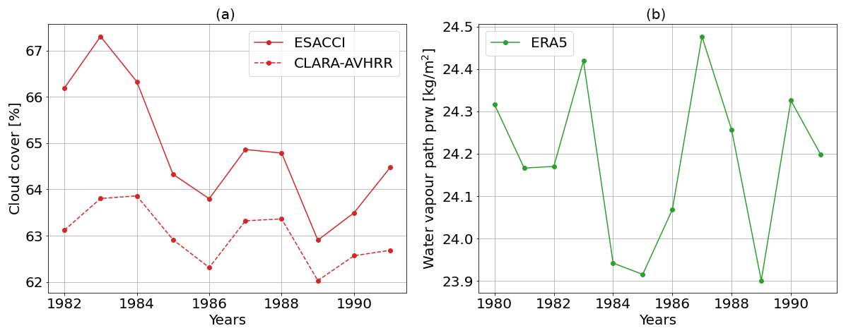
Figure A1 Time series of the observational products used for the cloud cover and the water vapour path.

Appendix B: Details on GP emulators and choice of the underlying hyperparameters

In this Appendix, we give a brief description of the Gaussian process (GP) regression framework used to construct emulators in this work and provide the relevant details regarding the hyperparameters used in their implementation. Gaussian processes are widely used in the context of Bayesian optimization as they are a method for describing distributions over unknown functions and can be efficiently updated or trained using samples from the ground-truth distribution (Rasmussen and Williams, 2005). In our case, the function we want to approximate with GP regression is that describing the dependence of a specific output Y of the climate model on a set of tuning parameters x, which we call Y_model(x). The output of a Gaussian process trained on set $\mathcal{T}=\mathit{\{}{\mathit{x}}_i,Y_{\mathrm{model}}({\mathit{x}}_i){\mathit{\}}}_i$ of ground-truth samples (ICON-A model runs, in our case) can be written as follows:

$$\begin{array}{}\text{(B1)}& f\left(\mathit{x}\right)|\mathcal{T}\sim \mathcal{G}\mathcal{P}\left(\mathit{\mu }(\cdot ),C_{\cdot ,\cdot }\right),\end{array}$$

where 𝒢𝒫 denotes the GP function distribution, with μ(x) and C being, respectively, the mean function and the covariance matrix that implicitly depend on 𝒯, i.e. that have been updated with the knowledge of the training data 𝒯 using Bayes' rule. Closed-form expressions for these functions are available and can be found in Rasmussen and Williams (2005). That is to say, given a new configuration x of tuning parameters, a GP trained on an ICON-A PPE for a given variable Y would output a normally distributed random variable with mean μ(x) and variance σ²(x) (which can also be explicitly calculated from the knowledge of the covariance matrix C (Rasmussen and Williams, 2005)). We therefore interpret μ(x) as our GP emulator prediction for Y and σ²(x) as the associated uncertainty and write

$$\begin{array}{}\text{(B2)}& {\displaystyle }& {\displaystyle }{Y}_{\mathrm{emul}}\left(\mathit{x}\right)\equiv \mathit{\mu }\left(\mathit{x}\right),\text{(B3)}& {\displaystyle }& {\displaystyle }\mathrm{Var}\left(Y_{\mathrm{emul}}\left(\mathit{x}\right)\right)\equiv {\mathit{\sigma }}^{\mathrm{2}}\left(\mathit{x}\right),\end{array}$$

which we use in Eq. (1) in the main text.

Importantly, the properties of the GP, particularly of the covariance matrix C, depend on the choice of a kernel function $k(\mathit{x},{\mathit{x}}^{\prime })$, which describes how the predictions at points x and x^′ are correlated. Kernel functions may also contain trainable hyperparameters, which are typically optimized by maximizing the log-marginal likelihood with respect to the training dataset (Rasmussen and Williams, 2005).

For our implementations, we used the GP regression library implemented in the scikit-learn package (https://doi.org/10.5281/zenodo.7711792, Grisel et al., 2024). We found Matèrn kernels to yield the highest prediction accuracy (which we measure via the R² coefficient). Matèrn kernels have two hyperparameters: a length scale l and a smoothness parameter ν. The length scale is typically the distance at which one can extrapolate outside the training data points: smaller values of l correspond to more rapidly varying functions that the GP can fit. This hyperparameter, together with the overall scale of the kernel, is optimized using the L-BFGS-B optimization (Jorge Nocedal, 2006) pre-implemented in scikit-learn. For the smoothness parameter ν, four values were tested: ν=0.5 corresponds to the absolute exponential kernel, ν=1.5 corresponds to a one-time differentiable function, ν=2.5 corresponds to a twice-differentiable function, and ν→∞ corresponds to a radial basis function (RBF) kernel. These four values of ν allow for a computational cost that is around 10 times smaller than that of the other values since they do not require us to evaluate the modified Bessel function (Rasmussen, 2006). The values of ν=2.5 and ν→∞ yield large negative R² scores and so are not represented here. In Fig. B1a, we observe a comparable performance of the GP emulator for ν=0.5 (absolute exponential kernel) and ν=1.5.

Other hyperparameters in the GP optimization are the noise level α (which can be interpreted as the variance of Gaussian noise added to the training data, with the aim of increasing the numerical stability of GP evaluations) and the number of random hyperparameter initializations for the log-marginal likelihood optimization (denoted with n_restart). Several values of α between 10⁻¹⁵ and 10⁻⁵ were tested. We show these tests in Fig. B1b. The values of $\mathit{\alpha }<{\mathrm{10}}^{-\mathrm{10}}$ yield large negative R² scores. A change in α for ${\mathrm{10}}^{-\mathrm{10}}<\mathit{\alpha }<{\mathrm{10}}^{-\mathrm{5}}$ does not have a significant effect on the performance of the GP emulator. Finally, we also tested several values of n_restart, between 0 and 100, as shown in Fig. B1c. From the tests presented in Fig. B1, the following values for the three hyperparameters are chosen (which are also default values in scikit-learn): ν=1.5, $\mathit{\alpha }={\mathrm{10}}^{-\mathrm{10}}$, and n_restart = 0.

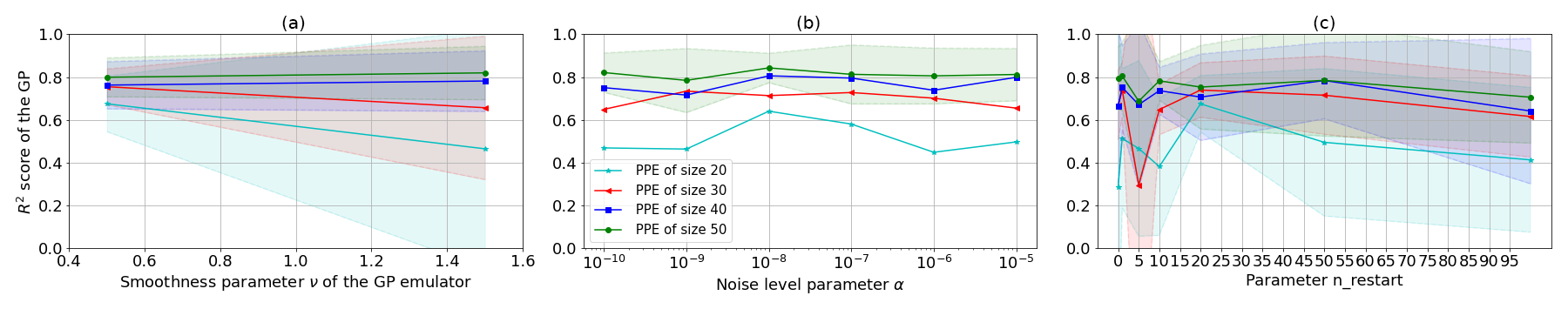
Figure B1 Performance (R² coefficient, calculated with 5-fold cross-validation) of the GP emulator with Matèrn kernel trained on PPE₁ and PPE₂ for different choices of hyperparameters: (a) for different values of ν, (b) for different values of α, and (c) for different values of n_restart.

Appendix C: Additional information on the generated PPEs

In this Appendix, we show additional data for the PPEs we generated in this work. Specifically, in Fig. C1, we show the sampled parameter values for PPE₃ (red circles) and PPE₄ (grey triangles), where signs of (slow) convergence in history matching are already visible after one iteration (with the distribution of the members of PPE₄ being slightly shifted and narrower). Figure C2 shows the sampled parameter values for PPE₅ (blue triangles), with the cyan square and red triangle marking the best-performing configurations reported in Table 7 in the main text.

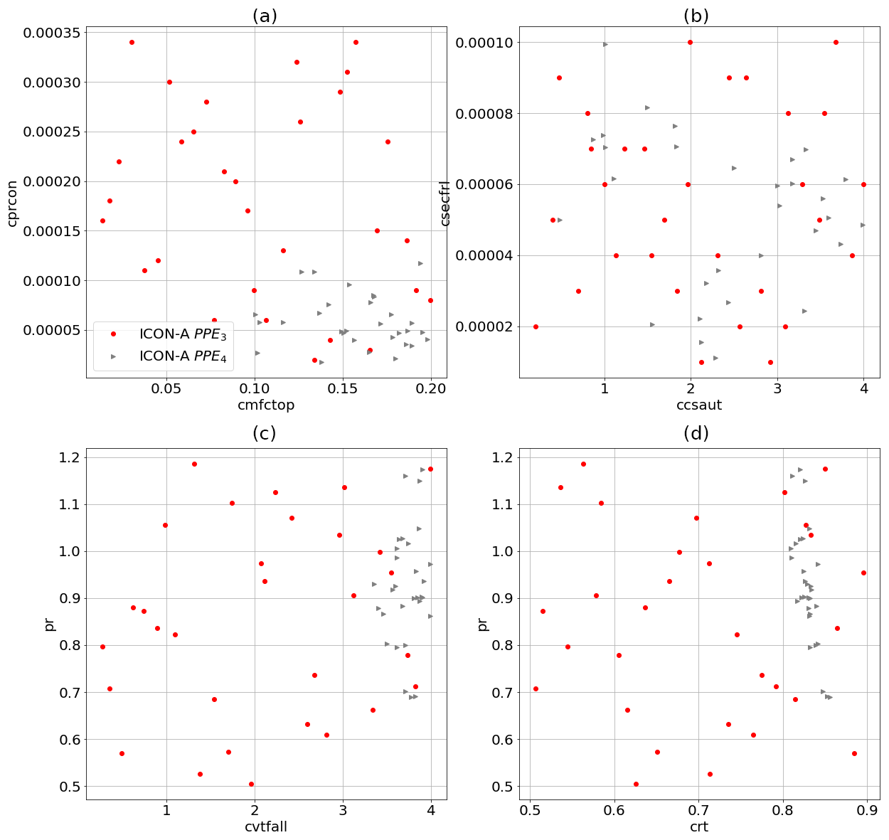
Figure C1 Sampled parameter values for PPE₃ (red circles) and PPE₄ (grey triangles). For each panel, two parameters are plotted on the two axes (see Table 3). The two PPEs are generated with parameter set 𝒫_p2. Signs of (slow) convergence of history matching are already visible after one iteration (with the distribution of the members of PPE₄ being slightly shifted and narrower). The extents of the plots includes all the PPE₄ values but not all of the PPE₃ values.

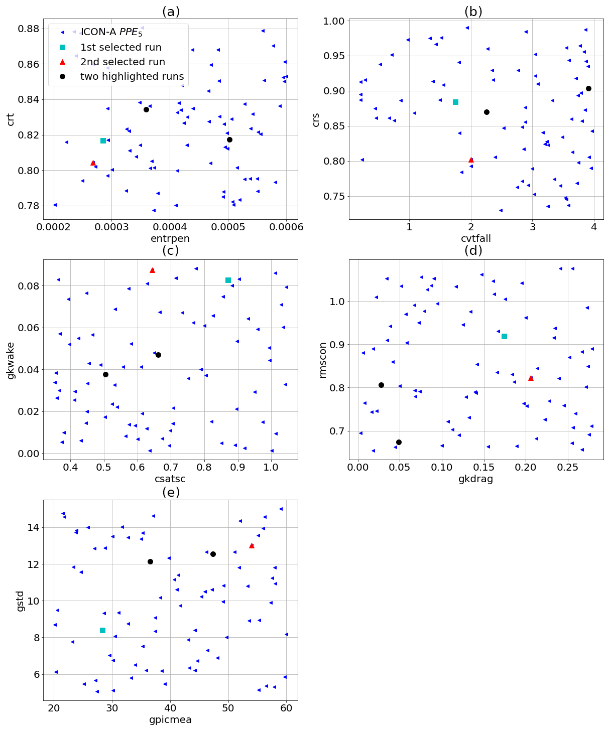
Figure C2 Sampled parameter values for PPE₅ (blue triangles). For each panel, two parameters are plotted on the two axes (see Tables 3 and 4). The PPE is generated with parameter set 𝒫_pd. Two selected PPE members corresponding to the best-performing configurations are highlighted (cyan square and red triangle).

Appendix D: Times series of the physics and dynamics metrics

In this Appendix, we show additional information complementing Fig. 9 in Sect. 3.2.1 in the main text. In Fig. D1, we show the yearly averages of the physics (top row, Fig. D1a–d) and dynamics (bottom row, Fig. D1e–h) output variables for the 30 runs of PPE₅ corresponding to Fig. 9. Also, in these time series, the higher year-to-year variability in the dynamics outputs compared to that in the physics ones can be clearly seen.

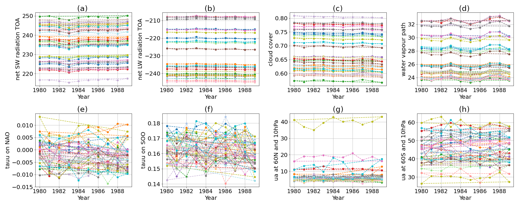
Figure D1 Time series (yearly averages) of the physics (top row, panels a–d) and dynamics (bottom row, panels e–h) output variables for 30 runs of PPE₅ (each colour corresponds to one run). The values for the years 1980 and 1989 are connected with a dashed line to help the reader identify the runs.

Appendix E: Additional information on parameter-to-output maps

In this Appendix, we show additional information on the parameter-to-output maps discussed in Sect. 3.2.3. In Fig.E1 (respectively, Fig. E2) we show the parameter-to-output map predicted with the GP emulators trained on PPE₁ and PPE₂, (respectively, PPE₃ and PPE₄) based on parameter set 𝒫_p1. (respectively, 𝒫_p2). In Fig. E2o–u, we can see that parameter set 𝒫_p2 does indeed allow for a higher (and closer to the observational values) global cloud cover compared to 𝒫_p1 (Fig. E1).

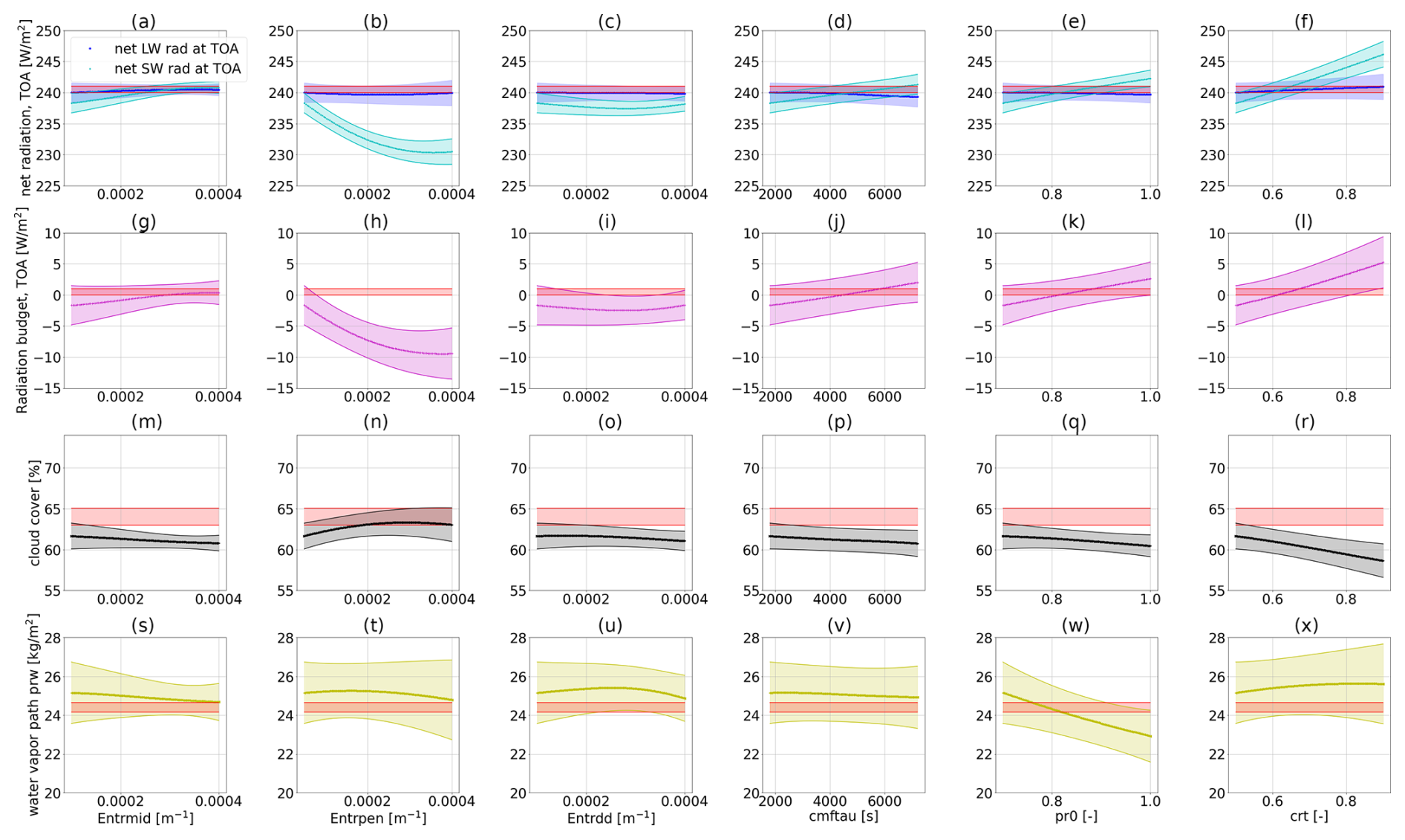
Figure E1 Parameter-to-output maps predicted with the GP emulators trained on PPE₁ and PPE₂. Every column corresponds to one tuning parameter being changed (see the list in Table 3), and every row corresponds to an output metric. The parameters that are not changed are kept fixed at their best-performing value from PPE₂ (marked with the magenta star in Figs. 2 and 3). The red-shaded areas in each plot denote the allowed output ranges from the observational data. The other coloured lines in each plot denote the emulator predictions (for the first row, dark and light blue denote the net longwave and shortwave radiation at TOA, respectively), with the corresponding uncertainty (1 standard deviation) represented as the shaded area.

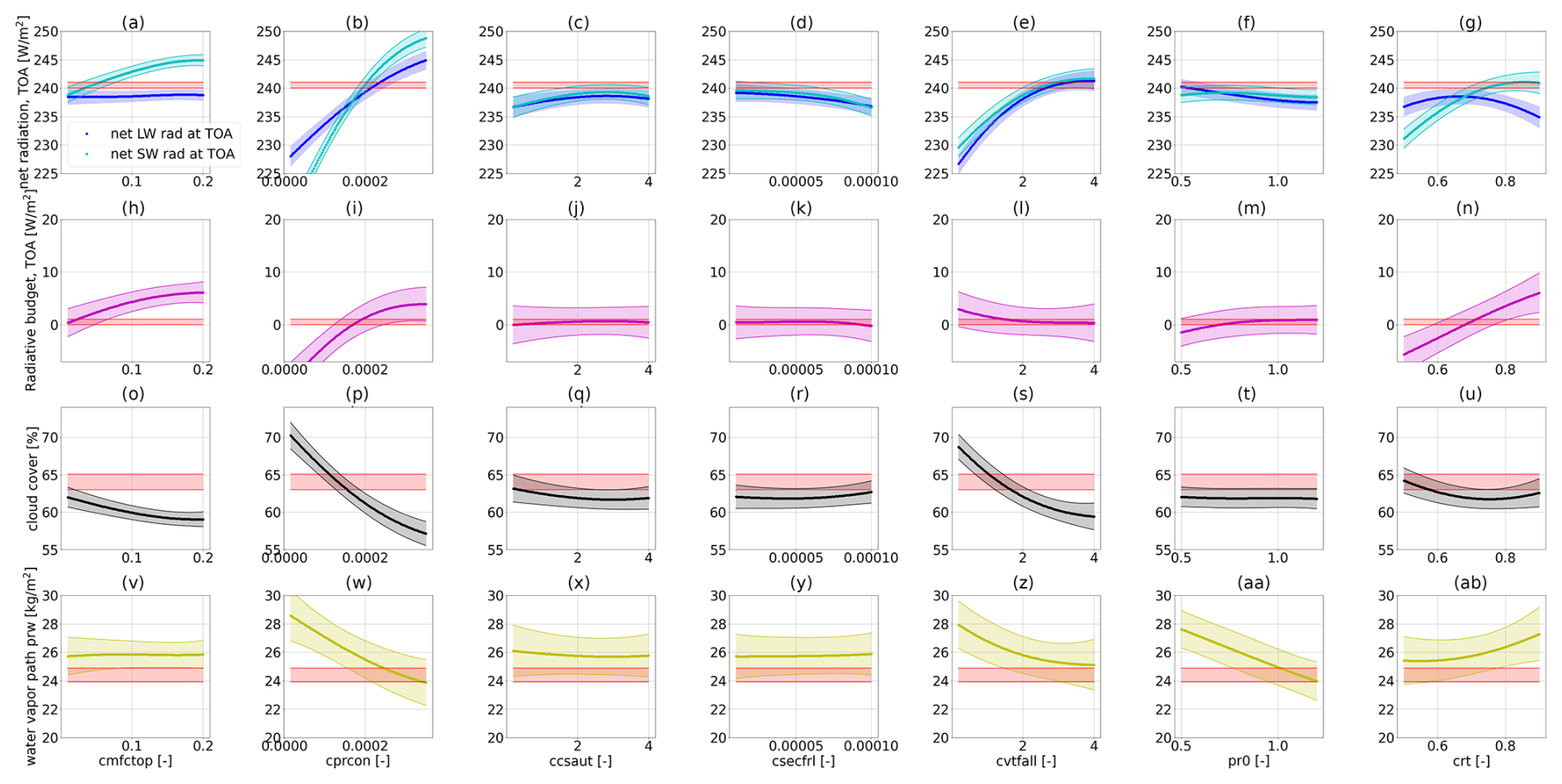
Figure E2 Parameter-to-output map predicted with the GP emulators trained on PPE₃ and PPE₄. Every column corresponds to one tuning parameter being changed (see the list in Table 3), and every row corresponds to an output variable. The parameters that are not changed are kept fixed at their best-performing value from PPE₂ (marked with the magenta star in Figs. 2 and 3). The red-shaded areas in each plot denote the allowed output ranges from the observational data. The other coloured lines in each plot denote the emulator predictions (for the first row, dark and light blue denote the net longwave and shortwave radiation at TOA, respectively), with the corresponding uncertainty (1 standard deviation) represented as the shaded area.