Reducing time and computing costs in EC-Earth: an automatic load-balancing approach for coupled Earth system models

Earth system models (ESMs) are intricate models employed for simulating the Earth's climate, typically constructed from distinct independent components dedicated to simulate specific natural phenomena (such as atmosphere and ocean dynamics, atmospheric chemistry, land and ocean biosphere). In order to capture the interactions between these processes, ESMs utilize coupling libraries, which oversee the synchronization and field exchanges among independent developed codes typically operating in parallel as a multi-program, multiple data (MPMD) application.

The performance achieved depends on the coupling approach, as well as on the number of parallel resources and scalability properties of each component. Determining the appropriate number of resources to use for each component in coupled ESMs is crucial for efficient utilization of the high-performance computing (HPC) infrastructures used in climate modeling. However, this task traditionally involves manual testing of multiple process allocations by trial and error, requiring significant time investment from researchers and making the process more error-prone, often resulting in a loss of application performance due to the complexity of the task. This paper introduces the automatic load-balance tool (auto-lb), a methodology and tool for determining the resource allocation to each component within coupled ESMs, aimed at improving the application's performance. Notably, this methodology is automatic and does not require expertise in HPC to improve the performance achieved by coupled ESMs. This is accomplished by minimizing the load imbalance: reducing each constituent's execution cost (core hours), as well as minimizing the core hours wasted resulting from the synchronizations between them, without penalizing the execution speed of the entire model. This optimization is achieved regardless of the scalability properties of each constituent and the complexity of their dependencies during the coupling.

To achieve this, we designed a new performance metric called “fittingness” to assess the performance of coupled execution, evaluating the trade-off between parallel efficiency and application throughput. This metric is intended for scenarios where optimality can depend on various criteria and constraints. Aiming for maximum speed might not be desirable if it leads to a decrease in parallel efficiency and thus increases the computational costs of simulation.

The methodology was tested across multiple experiments using the widely recognized European ESM, EC-Earth3. The results were compared with real operational configurations, such as those used for the Coupled Model Intercomparison Project Phase 6 (CMIP6) and European Climate Prediction project (EUCP), and validated on different HPC platforms. All of them suggest that the current approaches lead to performance loss, and that auto-lb can achieve better results in both execution speed and reduction of the core hours needed. When comparing to the EC-Earth standard-resolution CPMIP6 runs, we achieved a configuration 4.7 % faster while also reducing the core hours required by 1.3 %. Likewise, when compared to the EC-Earth high-resolution EUCP runs, the method presented showed an improvement of 34 % in the speed, with a 6.7 % reduction in the core hours consumed.

1 Introduction

In the field of climate science, the adoption of advanced modeling techniques has become imperative for understanding and predicting the complex dynamics of our planet's climate system. Recognition of the complex interconnectedness among various natural phenomena, crucial for describing the climate, led to the development of coupled general circulation models (CGCMs) more than 40 years ago, as illustrated by Manabe et al. (1975). These models captured the physical processes occurring in both the atmosphere and ocean. To further represent the natural feedback loops and avoid using predefined data on the given region by boundary conditions led to the creation of Earth system models (ESMs), which seek to simulate all relevant aspects of the Earth system, expanding the limits of CGCMs by simulating carbon cycle, aerosols, and other chemical and biological processes (Valcke et al., 2012; Lieber and Wolke, 2008). Consequently, coupling multiple codes that simulate different natural phenomena has become a common practice to better represent the climate.

Various strategies exist for designing the coupling approach in ESMs. Frequently, multiple independently developed codes run simultaneously and synchronize during the runtime to exchange fields with one another. These applications are commonly referred to as multi-program, multiple data (MPMD), and components running in parallel can employ different parallel paradigms such as Message Passing Interface (MPI; Tintó Prims et al., 2019) to take advantage of the HPC machines.

Achieving “satisfactory” performance on coupled ESMs is challenging, given the inherent complexities of such applications, but also of upmost importance to maximize the number of simulations and the resolution available to the climate research community, while using HPC infrastructures more efficiently. Balaji (2015) showed that current ESM performance is deteriorated due to the need for coupling. Acosta et al. (2023a) showed in a collection of performance metrics from multiple Coupled Model Intercomparison Project Phase 6 (CMIP6) experiments that the coupling cost adds, on average, a computational overhead (in core hours) of 13 %. As illustrated in Fig. 1, coordination among components is required to exchange the coupling fields, typically utilizing MPI. This often results in faster components waiting for the slower ones, a problem known as load imbalance. Moreover, extra computation is needed to transform the data between components using different grids, a process known as interpolation. This process, along with the associated MPI communications, has been studied extensively by Donners et al. (2012) to evaluate both the efficiency of the interpolation algorithm and the impact of these communications on overall performance. Minimizing the cost associated with the load imbalance by finding the appropriate resource configuration is a non-trivial process, which includes analyzing the speed-up of individual components at various processor counts, study their interactions during the coupling, and making trade-offs between the computing cost (core hours) and execution time of the coupled ESM.

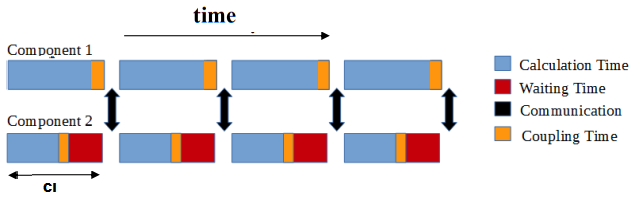
Figure 1 Overview of the typical timeline pattern observed between two coupled components during execution. Component 2 exhibits a faster computational time (depicted in blue) than Component 1, leading to Component 2 waiting at the end of each coupling interval (CI, depicted in red). The figure also illustrates the extension of the entire execution due to coupling time (depicted in orange). This typically includes tasks such as regridding and additional calculations necessary before communicating fields across different components.

The strategies for load-balancing ESMs can be divided into dynamic load balancing, where the load imbalance is minimized during the runtime, and static load balancing, where the process involves stopping and rerunning model execution to find resource configurations that minimize the coupling cost. To deal with the load balance “dynamically” the applications must allow reallocating the processes on which it runs during runtime, a property known as malleability (Feitelson and Rudolph, 1995). Some examples of using checkpoints during execution have been shown by Vadhiyar and Dongarra (2003) and Maghraoui et al. (2005, 2007). Possibly the most notable contributions to dynamic approaches have been done by Kim et al. (2011) to extend the Model Coupling Toolkit (MCT) to create the Malleable Model Coupling Toolkit (MMCT), enabling malleability and incorporating a load-balance manager module. This module decomposes the time of each component during a coupled interval (CI) into constituent computation and constituent coupling. The load-balance manager reallocates processing elements (PEs) from the fastest (donor) to the slowest (recipient) component until solution improvement ceases. This work was further enhanced in Kim et al. (2012b), where MMCT was extended with a prediction mechanism that maintains a database of PE execution times at each iteration, and a manually generated heuristic optimization to determine new resource configurations that reduce the coupling step execution time. Kim et al. (2012a) extended this approach to handle applications which have varying workloads during the execution.

However, the manually generated heuristic used for the prediction – based on static and manual inspection of coupled model interaction patterns and constituents’ computations – becomes impractical for more complex, realistic coupled models. To address this, Kim et al. (2013) proposed an instrumentation-based approach that collects runtime data from the constituents, demonstrating how this information can be used to improve coupling performance and accelerate the load-balancing decision-making process.

While these approaches have demonstrated significant improvements, they are designed for a highly flexible coupling scheme applicable only to climate models that adopt the MMCT extension of MCT. As a result, they are not suitable for most state-of-the-art ESMs. Moreover, the method proposed has not been validated with production ESMs used in climate research, but rather with a simplified “toy” model that mimics a simulation of the Community Earth System Model (CESM).

In contrast, our proposed solution is not integrated into any specific coupler, making it readily accessible to most ESMs used by the climate research community that employ an external coupling library to link multiple binaries (MPMD) into a single application.

It is essential to note that all these dynamic load-balancing methods rely on the ability to adjust the number of processes a constituent uses during the runtime, a feature that is rarely seen in state-of-the-art ESMs. Additionally, the method testing has been confined to toy models, lacking validation on ESMs widely employed within the scientific community. These limitations underscore the need for further research and adaptation to real-world, complex scientific applications. Furthermore, one can argue that these solutions are not as fully “dynamic” as suggested, given that the simulation has to be continuously interrupted during the runtime to collect the performance metrics, execute an algorithm to find a better setup, and resume the simulation. A truly dynamic approach should instead have other means to balance the workload to minimize the idle time such as tasks, an option explored with the Dynamic Load Balance library developed at the Barcelona Supercomputing Center (BSC). Garcia et al. (2009) and Marta et al. (2012) have explored the possibility of using this tool to reassign computation resources of blocked processes to more loaded ones to speed up hybrid MPI+OpenMP and MPI+SMPS applications. Although this is a promising option for the future, the current state of the tool still has room for improvement and thread-level parallelism is not common in the current generation of ESMs.

Static load-balancing solutions are well suited to the climate science community due to the difficulties found in applying dynamic approaches effectively. One of the most significant contributions of static load-balancing is the work by Ding et al. (2014, 2019) for CESM, which introduced an auto-tuning component integrated into the CESM framework to optimize process layout and reduce model runtime. It achieves this by employing a depth-first search method with a branch-and-bound algorithm to solve a mixed integer non-linear programming (MINLP) problem, combined with a performance model of the model components to minimize search overhead. This approach improves upon the earlier method described by Alexeev et al. (2014), which relied on a heuristic branch-and-bound algorithm and a less accurate performance model. Later, Balaprakash et al. (2015) proposed a static, machine-learning-based load-balancing approach to find high-quality parameter configurations for load balancing the ice component (CICE) of CESM. The method involves fitting a surrogate model to a limited set of load-balancing configurations and their corresponding runtimes. This model is then used to efficiently explore the parameter space and identify high-quality configurations. Their approach had to take into account the six key parameters that influence CICE component performance: the maximum number of CICE blocks and the block sizes in the first and second horizontal dimensions (x,y); two categorical parameters that define the decomposition strategy; and one binary parameter that determines whether the code runs with or without a halo. They demonstrated that their approach required six times fewer evaluations to identify optimal load-balancing configurations compared to traditional expert-driven methods for exploring feasible parameter configurations.

Importantly, coupling in CESM follows an integrated coupling framework strategy (Mechoso et al., 2021), where the climate system is divided into component models that function as subroutines within a single executable and are orchestrated by a coupler main program (CPL7), which coordinates the interaction and time evolution of the component models. The coupler also allows for flexible execution layouts, enabling components to run sequentially, concurrently, or in a hybrid sequential/concurrent mode. This coupling strategy differs from approaches that use an external coupler (such as OASIS, MCT, or YAC), where existing model codes are minimally modified to interface with the coupling library and executed as separate binaries on different physical cores, either interleaved or concurrently. Furthermore, the performance model used requires generating and analyzing execution traces to characterize the computation and communication patterns of key kernels for each coupled component separately. While this can provide more accurate performance representations, it also introduces significant challenges in adapting the approach to new components or other ESMs.

Other static solutions, such as those proposed by Will et al. (2017) for the COSMO-CLM regional climate model and Dennis et al. (2012) for CESM, demonstrate that load balancing in widely used ESMs can be approached in a relatively simple manner. These methods aim to identify a resource configuration where all individual components run at roughly the same speed, often constrained by a predefined parallel efficiency threshold. However, as we will show, this approach can easily lead to suboptimal solutions.

In this work, we present a static load-balancing method, automatic load balance (auto-lb), designed to improve resource allocation in coupled ESMs. Our approach is suited to coupled models that do not support malleability, where each component runs on a separate core as an MPMD application. Unlike other methods, our approach completely eliminates the need to modify any of the component's source codes; instead, it achieves load balance by adjusting the allocation of PEs assigned to each component. To accomplish this, we have introduced two new performance metrics: the Partial Coupling Cost to quantify the cost of the coupling per component, and the fittingness metric to better address the energy-to-solution (ETS, i.e., minimize the energy consumption) and time-to-solution (TTS, i.e., minimize the execution time) trade-off prevalent in all imperfectly scalable applications (Abdulsalam et al., 2015). These advancements set our method apart from existing approaches that either focus exclusively on minimizing execution time (pure TTS) or enforce parallel efficiency thresholds that limit speed in an arbitrary manner.

Moreover, the method includes a prediction phase capable of accurately estimating coupling performance based solely on the scalability properties of the individual model components. Unlike prior work, this eliminates the need for instrumenting the code, using profiling software, or trace generation. The results of the prediction phase allow our approach to significantly reduce the number of real simulations (and thus computational resources) required to determine an improved load-balancing configuration.

Finally, the method is fully integrated in a workflow manager, ensuring that the process of identifying the best resource configuration requires minimal user intervention and aligns with standard practices in climate modeling.

Our research primarily focuses on optimizing real experiment configurations for one of the most prominent European ESMs, EC-Earth3 (Döscher et al., 2022). Notably, EC-Earth3 employs the OASIS-MCT coupler (Craig et al., 2017), a widely used coupler also adopted by numerous other ESMs, particularly in Europe. The new methodology has been used to optimize configurations for different resolutions of EC-Earth3 experiment, including the same experiment configuration used for the CMIP6 exercise (Eyring et al., 2016), and the results of balancing a European Climate Prediction project (EUCP) high-resolution experiment on the European Centre for Medium-Range Weather Forecasts (ECMWF) Common Component Architecture (CCA) machine. This demonstrates that the method can be used across different machines and for different model resolutions, and of its potential applicability to a wide range of ESMs. The method has proven effective, yielding resource configurations that outperform the previous configurations in both execution time and computing cost. As detailed in Sect. 5, when compared to the setup used by the standard-resolution EC-Earth3 CMIP6 runs, we identified a new resource allocation that runs 4.7 % faster while reducing the core hours consumed by 1.3 %. Moreover, compared to the performance achieved by the EC-Earth3 high-resolution configuration used in EUCP, we achieved a reduction of the execution speed by up to 34 %, with a 6.7 % reduction in the core hours needed.

2 ESM under study: EC-Earth3

EC-Earth3 is a global coupled climate model developed by a consortium of European research institutions that integrates multiple component models to simulate the Earth system. Its goal is to build a fully coupled atmosphere–ocean–land–biosphere model usable for problems encompassing from seasonal-to-decadal climate prediction to climate change projections and paleoclimate simulations. Figure 2 shows an overview of the most commonly used EC-Earth3 configuration, EC-Earth3 at standard resolution (EC-Earth3 SR), which couples the ocean (NEMO), the atmosphere (IFS), and the runoff (RNF) components via the OASIS3-MCT coupler. In addition, a parallel I/O server (XIOS) is used to better handle the output of the oceanic component. The components are the following.

• The OASIS3-MCT coupler: a coupling library to be linked to the component models and whose main function is to interpolate and exchange the coupling fields between them to form a coupled system.

• The Integrated Forecasting System (IFS) as atmosphere model: an operational global meteorological forecasting model developed and maintained by the ECMWF. The dynamical core of IFS is hydrostatic, two-time-level, semi-implicit, semi-Lagrangian, and applies spectral transforms between grid-point space and spectral space. In the vertical the model is discretized using a finite-element scheme. A reduced Gaussian grid is used in the horizontal.

• The Nucleus for European Modelling of the Ocean (NEMO) as ocean model: a state-of-the-art modeling framework for oceanographic research, operational oceanography seasonal forecast, and climate studies. It discretizes the three-dimensional Navier–Stokes equations, being a finite difference, hydrostatic, primitive equation model, with a free sea surface and a non-linear equation of state in the Jackett. The ocean general circulation model (OGCM) is OPA (Océan Parallélisé), a primitive equation model that is numerically solved in a global ocean curvilinear grid known as ORCA. EC-Earth 3.3.2 uses NEMO version 3.6 with XML Input/Output Server (XIOS) version 2.0, an asynchronous input/output server used to minimize previous I/O problems.

• The Louvain-la-Neuve sea-Ice Model 3 (LIM3): a thermodynamic-dynamic sea-ice model directly coupled with OPA.

• The Runoff-mapper (RNF) component: used to distribute the runoff from land to the ocean through rivers. It runs using its own binary, coupled through OASIS3-MCT.

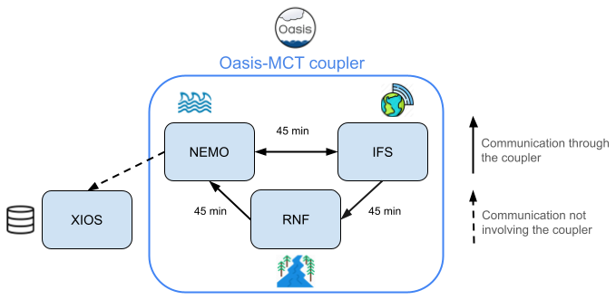
Figure 2 Overview of an EC-Earth3 experiment using the Nucleus for European Modelling of the Ocean (NEMO) as the ocean (with sea ice and ocean biogeochemistry), the Integrated Forecasting System (IFS) as the atmosphere, and the Runoff-mapper (RNF) as the runoff from land to the ocean. Furthermore, we include the XML I/O Server (XIOS) component, which is used by NEMO to provide asynchronous and parallel input/output operations. The arrows show the dependencies between components and the frequency of these interactions in simulated time. Note that XIOS does not communicate through OASIS-MCT. The coupling frequency depicted (45 min) corresponds to the standard resolution configuration (T255-ORCA1). Higher resolutions use higher coupling frequencies (e.g., 15 min for T511-ORCA025).

2.1 Experiment configurations

The configurations under study are the standard resolution (SR) and high resolution (HR) simulations (Döscher et al., 2022). They are the most used on EC-Earth3 and, therefore, the ones that consume more computing resources and for which any gain in performance has a greater impact. They both include IFS coupled with NEMO as the main components, parallelized using MPI, and which interchange 23 fields (6 from NEMO to IFS and 17 from IFS to NEMO) through OASIS3-MCT at the beginning of their own time step. As a consequence, the two components have to be synchronized before starting their own computation.

In SR, IFS uses the T255L91 grid, which corresponds to a resolution of 80 km for the atmosphere, coupled to NEMO using an ORCA1L75 grid, which corresponds to a 1° resolution at the Equator, or ∼ 25 km (Döscher et al., 2022). In HR configurations, the grids are T511L91 for the atmosphere and ORCA025 for the ocean, which correspond to a resolution of 40 km and $\mathrm{1}/\mathrm{4}$ of a degree for IFS and NEMO, respectively (Haarsma et al., 2020). They both involve, in addition to NEMO and IFS, the RNF and XIOS components. XIOS and RNF are not taken into account for load balancing, as XIOS does not communicate via OASIS but directly with NEMO to handle its I/O operations in parallel, and RNF runs in serial and is much faster than the other components.

3 Coupled ESM performance

ESMs are not an exception when it comes to their scaling properties: parallel efficiency cannot be maintained as we increase the number of PEs used. Thus, boldly selecting the configuration that maximizes speed leads to a waste of computing resources and is usually avoided. Consequently, efficiency metrics are used to evaluate how the execution cost (i.e., core hours) increases when adding more resources to an imperfect scalable model. In other words, how the speed-up of the application responds to the increase of parallel resources for a fixed problem size. Therefore, selecting the appropriate number of PEs to execute the program becomes a trade-off between the speed (TTS) and the core hours (ETS) required for execution, and the proper decision can vary depending on the context: computing resources available, HPC infrastructure policies, scheduling configurations and constraints, and urgency for getting the results. As seen by Acosta et al. (2023a), another key factor that further deteriorates computational performance in current ESMs is the coupling between their components. This overhead stems from faster components having to wait for slower ones during synchronization, a phenomenon known as load imbalance, as well as the additional computation required to interpolate data between components operating on different grids.

Previous work by Acosta et al. (2023b) has studied this in the context of the EC-Earth3 model, showing that while the interpolation process adds to the coupling cost, most of the overhead comes from synchronization delays. Minimizing these costs is crucial to improving the overall performance of the coupled system. However, reducing load imbalance by optimizing resource allocation across components is a complex task. It requires compromising on the parallelization of individual components to minimize the waiting time during synchronizations. In doing so, we limit the ability to freely choose the best resource configuration for each component, which means some parallel efficiency is lost on the individual components due to not using their best scalability point, but rather the one that bests suits the whole ESM.

This section introduces the performance metrics used during our work to assess the performance of coupled ESMs, as well as presenting both the problem and adopted solution for the ETS/TTS trade-off.

3.1 Performance metrics

On the one hand, there are very well-known speed-up and parallel efficiency metrics – widespread metrics used to assess the performance achieved while dealing with the same amount of work but with different processor counts (scalability with fixed problem size). Given that some of the ESM components cannot run in a single process (serial execution) due to memory and/or computing requirements, execution in a single node per component (p_o) is taken as the baseline instead. Therefore, the speed-up at p processors is defined as

$$\begin{array}{}\text{(1)}& {\text{Speedup}}_p={\displaystyle \frac{T_{p_o}}{T_p}},\end{array}$$

where T_p is the execution time using p processes.

Likewise, the parallel efficiency at p processes is defined as

$$\begin{array}{}\text{(2)}& {\text{Efficiency}}_p={\displaystyle \frac{{\text{Speedup}}_p}{p/p_o}}.\end{array}$$

On the other hand, we use a subset of the performance metrics specially designed for the common structure of ESMs and how they are executed in production: the Computational Performance Model Intercomparison Project (CPMIP, Balaji et al., 2017). Those of particular interest for our analysis are:

• Simulated years per day of execution (SYPD). The number of simulated years (SY) by the ESM within a single execution day, defined as 24 h of computation time on the HPC platform.

• Core hours per simulated year (CHSY). The core hours per simulated year. Measured as the product of the model runtime for 1 SY (in hours) and the number of cores allocated (P_M). Note that CHSY and SYPD are related:

  $$\begin{array}{}\text{(3)}& \mathrm{CHSY}={\displaystyle \frac{\mathrm{24}\cdot P_{\mathrm{M}}}{\mathrm{SYPD}}}.\end{array}$$

• Coupling cost (Cpl_cost). Measures the overhead caused by the coupling. This can be due to the waiting time caused by the synchronization between models within the ESM (faster components have to wait for slower ones), the added cost of interpolating the data from the source grid to the target one, and the time spent in communications when sending/receiving the data (see Fig. 1).

  $$\begin{array}{}\text{(4)}& \text{Cost}={\displaystyle \frac{T_{\mathrm{M}}{P}_{\mathrm{M}}-{\sum }_c{T}_{\mathrm{C}}{P}_{\mathrm{C}}}{T_{\mathrm{M}}{P}_{\mathrm{M}}}},\end{array}$$

  where T_M and P_M are the runtime and parallelization for the whole model, and T_C and P_C the same for each component.

  For this work, Eq. (4) has been reformulated to evaluate how much each component adds to the coupling cost, which is essential to knowing which component should lend PEs, and which one should receive them. It has been called the partial coupling cost:

  $$\begin{array}{}\text{(5)}& \mathrm{Partial}\mathrm{\_}\mathrm{cpl}\mathrm{\_}\mathrm{cost}={\displaystyle \frac{T_{\text{Ccpl}}{P}_{\mathrm{C}}}{T_{\mathrm{M}}{P}_{\mathrm{M}}}},\end{array}$$

  where T_Ccpl is the total time spent by a component in coupled events (waiting, interpolating, and sending).

All these metrics are collected after the simulation using runtime timing information provided by the load balance tool integrated in OASIS3-MCT (Maisonnave et al., 2020).

3.2 Time-to-solution vs energy-to-solution criteria

If we want an application to run faster, we will increase the number of PEs. Assuming that the parallel efficiency decreases (due to imperfect scalability), the core hours consumed by the application will rise. Given that the core hours are directly proportional to the energy cost of execution, they directly influence energy consumption (Balaji et al., 2017). This is known in the literature as the TTS vs ETS trade-off (Freeh et al., 2005).

One of the most commonly used metrics for assessing program performance, which considers both execution time and the parallel efficiency, is the energy-delay product (EDP). In the context of MPI applications, the EDP can be computed as follows (Yepes-Arbós et al., 2016; Abdulsalam et al., 2015):

$$\begin{array}{}\text{(6)}& \mathrm{EDP}=\mathrm{Speedup}\cdot \mathrm{Efficiency}.\end{array}$$

In this study, we introduce a novel metric termed “fittingness” (FN) that enables the parameterization of the time–energy trade-off at which a program is intended to operate. This metric serves as a valuable tool for assessing and optimizing program performance by considering the balance between execution time and energy consumption. To that end, we initially define two parameters: time-to-solution weight (TTS_w) and energy-to-solution weight (ETS_w). Both parameters are constrained to a range between 0 and 1, and their sum must equal unity:

$$\begin{array}{}\text{(7)}& {\mathrm{TTS}}_{\mathrm{w}}+{\mathrm{ETS}}_{\mathrm{w}}=\mathrm{1}.\end{array}$$

Then, given the scalability curve of one component, with the SYPD (metric of execution time) and CHSY (metric of execution cost) at different core counts, the FN is calculated as follows:

$$\begin{array}{}\text{(8)}& \mathrm{FN}={\mathrm{TTS}}_{\mathrm{w}}\cdot {\mathrm{SYPD}}_{\mathrm{n}}+{\mathrm{ETS}}_{\mathrm{w}}\cdot (\mathrm{1}-{\mathrm{CHSY}}_{\mathrm{n}}),\end{array}$$

where SYPD_n (CHSY_n) is the value of the SYPD (CHSY) after a min–max normalization, which is performed across all tested configurations. Note that we use 1−CHSY_n given that the greater the cost, the less energy efficient the execution will be. In other words, lower costs correspond to improved energy efficiency during execution. Consequently, minimizing the cost not only enhances performance but also reduces consumption of core hours.

Weighting the SYPD (CHSY) with TTS_w (ETS_w) enhances the flexibility in determining the resource configuration that better suits the specific requirements of climate scientists.

Table 1 and Fig. 3 show how the FN metric compares to the EDP across different TTS_w for the atmospheric component (IFS) in SR. The SYPD_n (CHSY_n) column is the value of the SYPD (CHSY) after a min–max normalization. For instance, using 48 PEs for IFS is the slowest configuration (SYPD_n=0) but the one that consumes least energy ($\mathrm{1}-{\mathrm{CHSY}}_{\mathrm{n}}=\mathrm{1}$). On the other hand, using 1008 PEs is the fastest configuration (SYPD_n=1) but the worst in terms of energy ($\mathrm{1}-{\mathrm{CHSY}}_{\mathrm{n}}=\mathrm{0}$).

Table 1 Comparison of fittingness (FN), parallel efficiency (Eff), and energy-delay product (EDP) metrics across different processor counts for the Integrated Forecasting System (IFS) atmospheric component. The results illustrate how the recommended parallelization for this component changes with the time-to-solution weight (TTS_w), ranging from 0.3 to 0.9. Bold values indicate the best parallelization choice for each TTS_w.

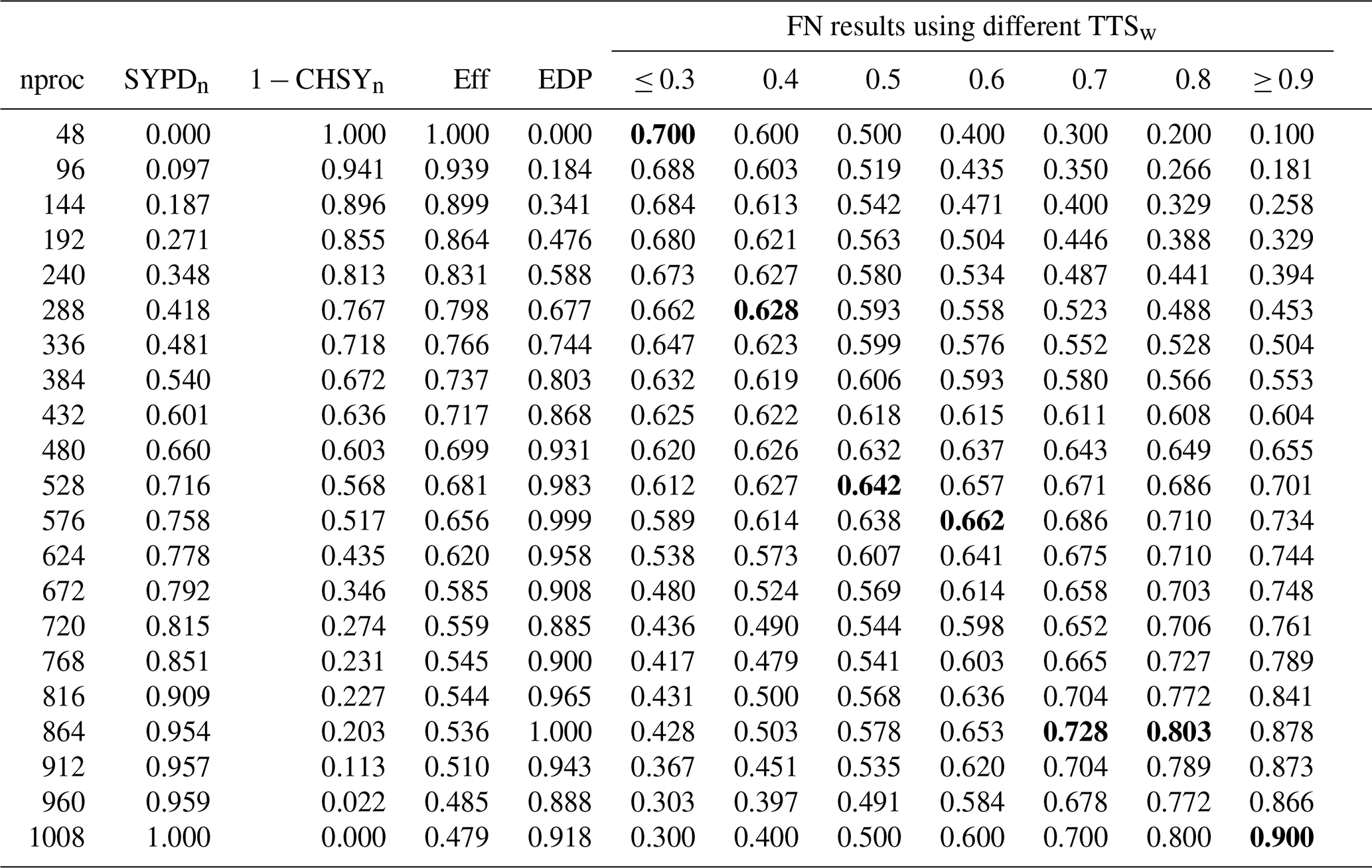
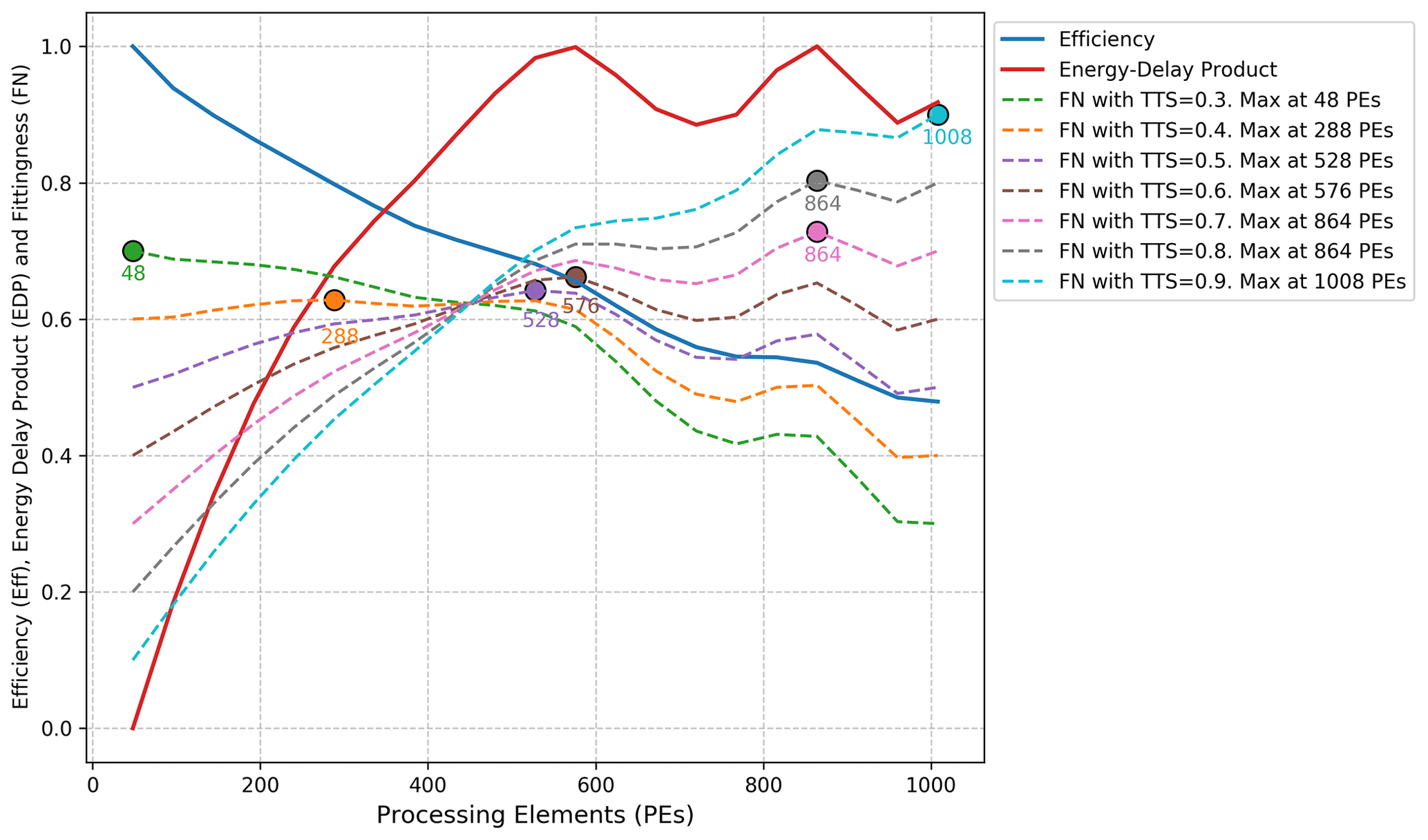
Figure 3 Efficiency (Eff), energy-delay product (EDP), and fittingness (FN) values for different processor counts for the Integrated Forecasting System (IFS) atmospheric component. The figure shows how the parallelization choice – defined as the configuration that maximizes FN – shifts from slower, more cost-effective options to faster but more expensive ones as the time-to-solution weight (TTS_w) increases from 0.3 to 0.9.

3.3 Model performance stability and measurement uncertainty

Evaluating the performance of ESMs inherently involves uncertainty due to the variability of HPC environments. Under an ideal scenario, repeated runs of the same model setup should yield identical runtimes. However, in practice, HPC systems experience fluctuations due to background system load, hardware failures, and network congestion. The HPC platform used, MareNostrum4, was continuously monitored, and Operations receive alerts when performance falls below expected levels. Any jobs executed during these periods can be identified and discarded to prevent skewed results. Additionally, and to further minimize the impact of these factors and ensure the reliability of our performance analysis, we followed these practices:

• Exclusive resource allocation. All jobs were submitted with the “-exclusive” clause, which ensures allocated nodes were not shared with other running jobs. This minimizes performance noise from co-scheduled workloads.

• Simulation length. We configured model runs to use longer simulation chunks, which helps smooth out machine performance fluctuations. Depending on the model speed, we chose different chunk sizes. For SR runs, we used 1-year chunks, whereas for HR using 3-month chunks was enough. In both cases each chunk has a runtime of ∼1 h.

• Multiple runs. Each resource configuration (chunk) was executed at least twice, and the results were averaged to mitigate fluctuations.

• Ignore the initialization and finalization phases. The initialization and finalization phases of an ESM run involve a higher proportion of I/O operations for reading initial conditions and writing outputs, making them less representative of sustained model performance. To account for this, we analyzed the runtime deviation of these phases compared to the regular time-stepping loop and found that discarding the first and last simulated day was sufficient to account only for the regular time steps. This was easily achieved using a dedicated parameter in the load balance analysis tool integrated in EC-Earth3 (Maisonnave et al., 2020).

• Run at different times during the day. To account for diurnal fluctuations in HPC load, experiments were executed at different times. This was not strictly enforced but naturally resulted from using a queue that allowed only one job per user at a time. Combined with varying queue wait times, this led to experiment jobs running at different times throughout the day.

• Manual and post-mortem validation. All reported results underwent manual validation. Additionally, once an optimized resource setup was identified, a duplicate run was performed to confirm that the observed performance improvement was consistent with the initial measurement.

4 Automatic load-balance method

This section describes auto-lb, a methodology and tool aimed at improving the performance of ESMs by determining the proper distribution of the HPC resources (PEs) allocated to each component in coupled executions. This is accomplished by minimizing the core hours lost due to synchronizations between interacting coupled components and by selecting a well-balanced speed for the coupled execution, considering the different scalability properties of the individual components. Additionally, given that different platforms and users may have varying constraints and criteria, the method can be used to find a solution within a restricted maximum number of PEs. It also allows users to define the priority between the achieved speed (TTS) and the core hours consumed (ETS), as described in Sect. 3.2. The methodology is described in more detail in Algorithm 1 and Fig. 4. It and can be divided into three main steps:

1. Get component's scalability. Obtain the SYPD (i.e., execution time) for each component involved in the coupled configuration using various PE counts. The goal is to have a real representation of the model's performance. Thus, it is recommended to take the metrics from a configuration as similar as possible to the coupled run (same resolution, modules, I/O, online diagnostics, compilation flags, etc.), and getting as close to the actual model performance. To minimize measurement uncertainties, we followed the best practices outlined in Sect. 3.3.

2. Prediction script. A Python script that, given the scalability curves of the components involved in the coupled configuration, returns the best resource allocation (i.e., how many PEs have to be assigned to each coupled component) depending on the user criteria (TTS or ETS) using the FN metric.

3. Load-balance workflow. Workflow that will submit multiple instances of the ESM on the HPC machine using an existing climate workflow manager called Autosubmit (Manubens-Gil et al., 2016). The workflow involves an iterative process, with each step involving the following: submitting multiple instances of the ESM, each with different resource configurations (initially, the resource allocation used is the one estimated as “optimal” by the Prediction script), collecting the performance metrics from each run, and making fine-grained modifications to the resource setup to reduce the coupling cost (i.e., including the waiting time due to synchronizations and the time spent performing interpolations on the fields being exchanged) of the ESM at the next iteration. The performance achieved by each run is stored, and the outcome of the workflow is the resource setup which outperformed all the others. To mitigate performance uncertainties that could affect the results, we applied the practices described in Sect. 3.3.

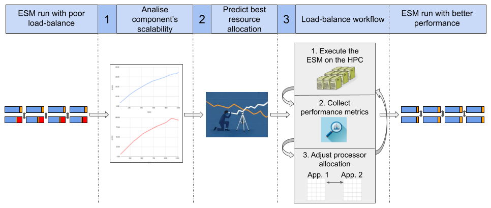
Figure 4 An overview of the auto-lb workflow, illustrating the steps to enhance the performance of an Earth system model (ESM) from an initially unbalanced configuration. The process begins with (1) obtaining the scalability properties of each component (scalability curve). These results are then used by (2) the Prediction script to estimate potential well-balanced resource configurations. Finally, these configurations are used in (3) to iteratively simulate multiple instances of the ESM to identify a solution that minimizes the coupling cost, potentially improving the SYPD (i.e., speed) and reducing the CHSY (i.e., computing cost) of the simulation.

4.1 Prediction script

The number of possible configurations that can be used in coupled ESMs is too large to individually test each one. Take, for instance, two-component systems like IFS–NEMO experiments, where both can utilize from 1 to 21 nodes. Using a granularity of one node, there are $\mathrm{20}\times \mathrm{20}=\mathrm{400}$ possible solutions. However, most of these configurations are completely unbalanced. Testing all of them is unnecessary and would result in a waste of resources with no added value.

The Prediction script can search this solution space in less than one second, approximating the results from each combination of PEs for IFS–NEMO based on the prior knowledge of the parallel behavior that we have from the scalability curves, thus finding the best setups for the TTS/ETS criteria selected. This not only ensures well-balanced setups but also considers potential high-quality parallelization regions for individual components.

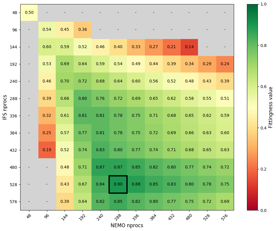
Figure 5 Fittingness matrix for IFS–NEMO coupled execution using a TTS_w of 0.5. The matrix shows the fittingness metric for various processes combinations, with IFS PEs in the vertical axis and NEMO PEs along the horizontal. Cells are color-coded from red (worst) to green (best), with gray indicating configurations worse than the baseline setup of 48 processes (equivalent to one node) per component.

Figure 5 illustrates the fittingness metric using a TTS_w of 0.5. The best solution found uses 528 PEs for IFS and 288 for NEMO. However, these results are derived from scalability curves rather than actual simulations, which means they might not account for all factors that influence HPC machine performance. The Prediction script addresses this by providing not just the single best configuration, but the top N possible configurations (to be set by the user). This approach balances the risk of limited search space if only one combination is considered against the impracticality of exploring every possible configuration. Analyzing the entire search space would be excessively time-consuming and computationally costly, potentially outweighing the gains of any performance analysis. For instance, and as detailed in Sect. 5, we have found that selecting the top five configurations provides a reasonable balance between total auto-lb runtime (around 24 h) and search space given the application studied (EC-Earth). In the given example (Fig. 5), the top five combinations are 528–288, 528–336, 480–240, 480–288, and 480–336 (IFS–NEMO). Extreme combinations with no practical benefit are grayed out, as their huge coupling cost (vast difference in execution time between the coupled components) makes them less performant than the baseline case (one node per component). These configurations are not worth further investigation.

The Prediction script will, therefore, serve as a guide for the load-balance workflow (Sect. 4.2) as now it won't have to search in the whole solution space but only in a relatively confined space to find the best resource configuration. This minimizes resource wastage by avoiding testing all possible combinations of PEs for IFS and NEMO and starting the in-depth analysis with some already potentially good setups.

4.2 Load-balance workflow

The load-balance workflow is an iterative process that consists of a loop that submits multiple instances of the experiment using different resource setups, from which it collects the metrics defined in Sect. 3. These metrics guide the redistribution of the computational resources assigned to each component in subsequent iterations to minimize the coupling cost while improving the overall performance. This reallocation policy relies on the partial_coupling_cost metric (Eq. 5), which identifies the component contributing the most to the coupling cost. The identified component, referred to as the donor, is the one underutilizing its allocated resources while waiting for coupling data from the other component, labeled as recipient. The number of PEs transferred between the donor and the recipient at the first (initial_step) and last (minimum_step) iterations is a user-defined parameter, and depends on the application's sensitivity to changes in the number of parallel resources. The outcome of the current iteration is a new set of resource configurations that will be submitted in the following iteration. The workflow is designed to guarantee convergence. If, at a given iteration, the direction of resource transfer changes (i.e., a previously identified recipient now becomes a donor), the step size is reduced by half. This iterative refinement continues until the step size falls below a user-specified threshold (minimum_step), at which point no further meaningful adjustments can be made. The workflow concludes when no new viable configurations can be explored or when further refinements produce negligible differences in performance. At this stage, the FN metric is evaluated across all tested configurations to determine the best resource allocation found.

Figure 6 provides an overview of a single workflow iteration that runs two instances per resource configuration.

Algorithm 1 Automatic load-balance method (auto-lb).

Given:

1:

A set of T independent tests with different resource configurations: $\mathit{\text{tests\_to\_explore}}=\mathit{\{}{\mathit{\text{test}}}_{\mathrm{0}},{\mathit{\text{test}}}_{\mathrm{1}},\mathrm{\dots },{\mathit{\text{test}}}_T\mathit{\}}$

2:

An initial step size: initial_step

3:

The minimum allowable step size: minmum_step

4:

A step size for each test, initially set to initial_step: $\mathit{\{}{\mathit{\text{step}}}_{\mathrm{0}},{\mathit{\text{step}}}_{\mathrm{1}},\mathrm{\dots },{\mathit{\text{step}}}_T\mathit{\}}=\mathit{\text{initial\_step}}$

5:

while tests_to_explore≠∅ do

6:

▹ Start lb_iter

7:

for each test in tests_to_explore do

8:

Submit the test to the HPC platform

▹ SIM job

9:

Collect the performance metrics

▹ POST job

10:

end for

11:

Identify the donor and recipient components

▹ Start LOAD_BALANCE job

12:

Define a new resource setup by reallocating S PEs from the donor to the recipient

13:

Check that the new resource setup has not been tested before

14:

if the new setup was executed before on any of the previous tests then

15:

Halve the step size for this test: ${\mathrm{step}}_i={\mathrm{step}}_i/\mathrm{2}$

16:

end if

17:

if step_i≥minimum_step then

18:

Submit test with the new configuration (jump to 7.)

19:

else

20:

Remove this test from tests_to_explore

21:

end if

▹ End LOAD_BALANCE job

22:

end while

▹ End lb_iter

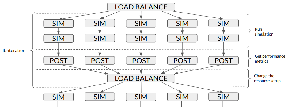
Figure 6 Overview of a single iteration of the load-balance workflow (lb-iteration). Five different resource configurations (SIM) are submitted, running two instances for each. The performance results are gathered in the POST_LUCIA job and the LOAD_BALANCE job will give resources from one component to the other to achieve a better-balanced configuration.

5 Results and discussion

In this section, we present the results of using the auto-lb tool for different configurations and experiments to demonstrate its effectiveness at improving ESM performance and its versatility across different resolutions and platforms. We begin by evaluating the standard-resolution EC-Earth3 configurations used in the CMIP6 exercise, highlighting how our tool improves upon configurations previously considered to be near-optimal. Next, we analyze high-resolution EC-Earth3 configurations used in the EUCP system, showcasing the tool's capability for handling scenarios that require significantly larger computational resources. Additionally, we explore how varying the trade-offs between TTS and ETS can yield different well-balanced configurations, depending on the specific needs of each experiment and the HPC platform. We also illustrate the portability of auto-lb by using it on different HPC platforms, such as MareNostrum4 and CCA, demonstrating its adaptability in improving ESM performance across diverse computational environments.

5.1 EC-Earth3 at standard resolution for CMIP6

During the CMIP6 project, even when accounting only for experiments used for production (not taking into account the spin-up runs), more than 240 000 years were simulated for multiple ESMs across different HPC platforms. At the BSC, an EC-Earth3 SR CMIP6 configuration was used to execute more than 14 000 years in MareNostrum4 (Acosta et al., 2023a); achieving the best performance was crucial for such a big project. An “optimal” resource configuration of 384 PEs for IFS and 240 for NEMO was agreed upon. This configuration resulted in a total number of PEs lower than 768. This value is significant because the scheduling policy permits jobs utilizing up to 768 PEs to access a “debug” queue. While this reduces queue time, it restricts the scheduler to allow no more than one job to run simultaneously for each HPC user. The average performance results for one chunk with this configuration was 15.29 SYPD, 1113 CHSY, and had a coupling cost of 14.81 %. Figure 7a shows the scalability of IFS. The model scales well until 350 processes and seems to saturate at 550. Figure 7b demonstrates that NEMO scales exceptionally well. The cost of adding more parallel resources remains negligible until 600 PEs. Beyond this point, the speed-up gains become less pronounced compared to earlier increments.

After setting up the experiment and obtaining the scalability curves for IFS and NEMO, the Prediction script was executed with the following parameters: max_nproc set to 672 (the maximum PEs for IFS and NEMO after subtracting the 95 used by XIOS and 1 used by RNF, $\mathrm{672}+\mathrm{95}+\mathrm{1}=\mathrm{768}$), and a TTS_w of 0.5. These parameters are explained in Sect. 4.1.

The Prediction script found the “optimal” solution to be 384 PEs for IFS and 264 for NEMO. The top five configurations are shown in Table 2. The result of the workflow is illustrated in Fig. 8. Tests from 0 to 4 are resource configurations given by the prediction script and test 5 is the original one. The load-balance workflow finished after 4 iterations and a total of 24 (6×4) resource configurations were tested. Note, however, that as shown in Fig. 8, four of the tests are repeated (lb-iter 3, tests 0, 3, 4, and 5). The total execution time of the workflow was 50 h. The best result is 408 IFS, 240 NEMO, which compared to the original configuration is 4.7 % faster (16.01/15.29) and 1.3 % less costly (1099/1113). The coupling cost grows from 14.81 % to 17.4 % but it is compensated by using a better number of PEs given NEMO and IFS scalability properties. If the resource configuration found by auto-lb had been used during the CMIP6 exercise, achieving a performance increase of 4.7 % in execution time is equivalent to reducing the simulated time by $\mathrm{14}\mathrm{020}/\mathrm{15.29}-\mathrm{14}\mathrm{020}/\mathrm{16.01}=\sim \mathrm{41}$ d (if the experiments were run by only one user). Similarly, a reduction of the cost by 1.3 % is equivalent to the cost of simulating 182 years.

The results also demonstrate the high accuracy of the Prediction script. As illustrated in the first row of Fig. 8, which shows the resource configurations provided by the Prediction script (lb-iter 0), tests 0, 1, 2, and 3 consistently outperform the original setup (lb-iter 0, test 5). Therefore, the only predicted configuration performing worse than the original is observed in test 4. It is noteworthy that Fig. 8 provides evidence that the iterative auto-lb phase leads to better resource setups. Following the evolution of test 4, after two lb-iterations (lb-iter 2, test 4) the auto-lb workflow achieved a new configuration that also outperforms the original one. Similarly, just one iteration after the original resource setup (lb-iter 1, test 5) shows that reallocating 48 processes from IFS to NEMO also provides a superior configuration compared to what was used in production during CMIP6.

Table 2 Top five initial resource configurations from the Prediction script to be used by the load-balance workflow for the SR CMIP6 experiment.

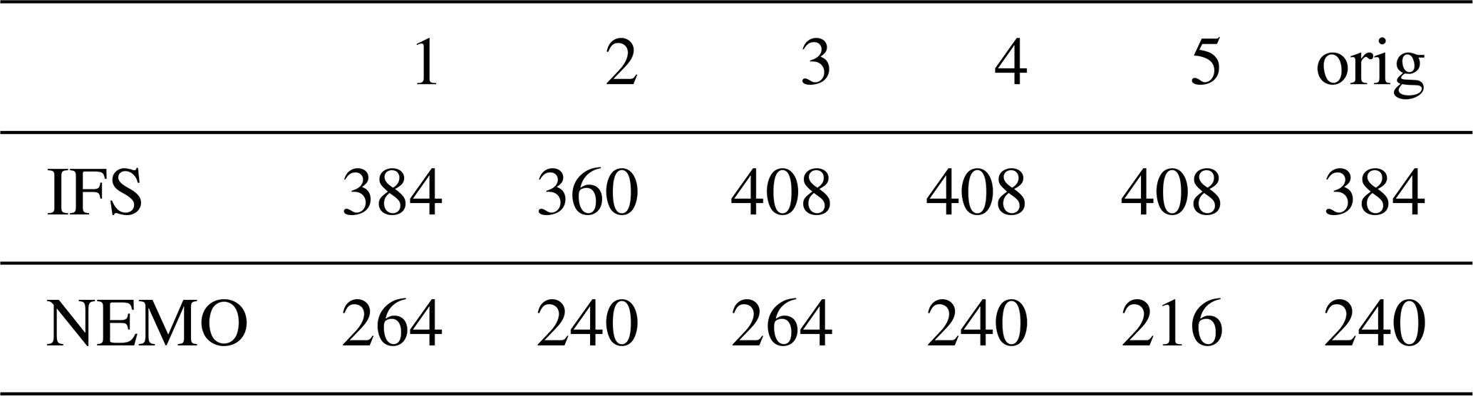
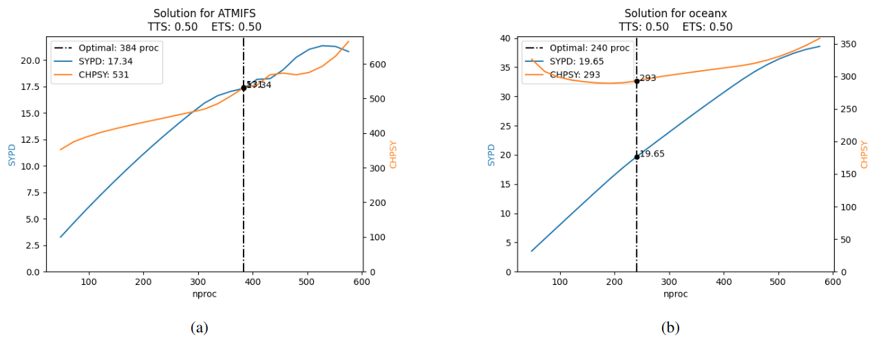
Figure 7 Scalability and predicted best resource allocation for IFS and NEMO at standard resolution for CMIP6 experiments.

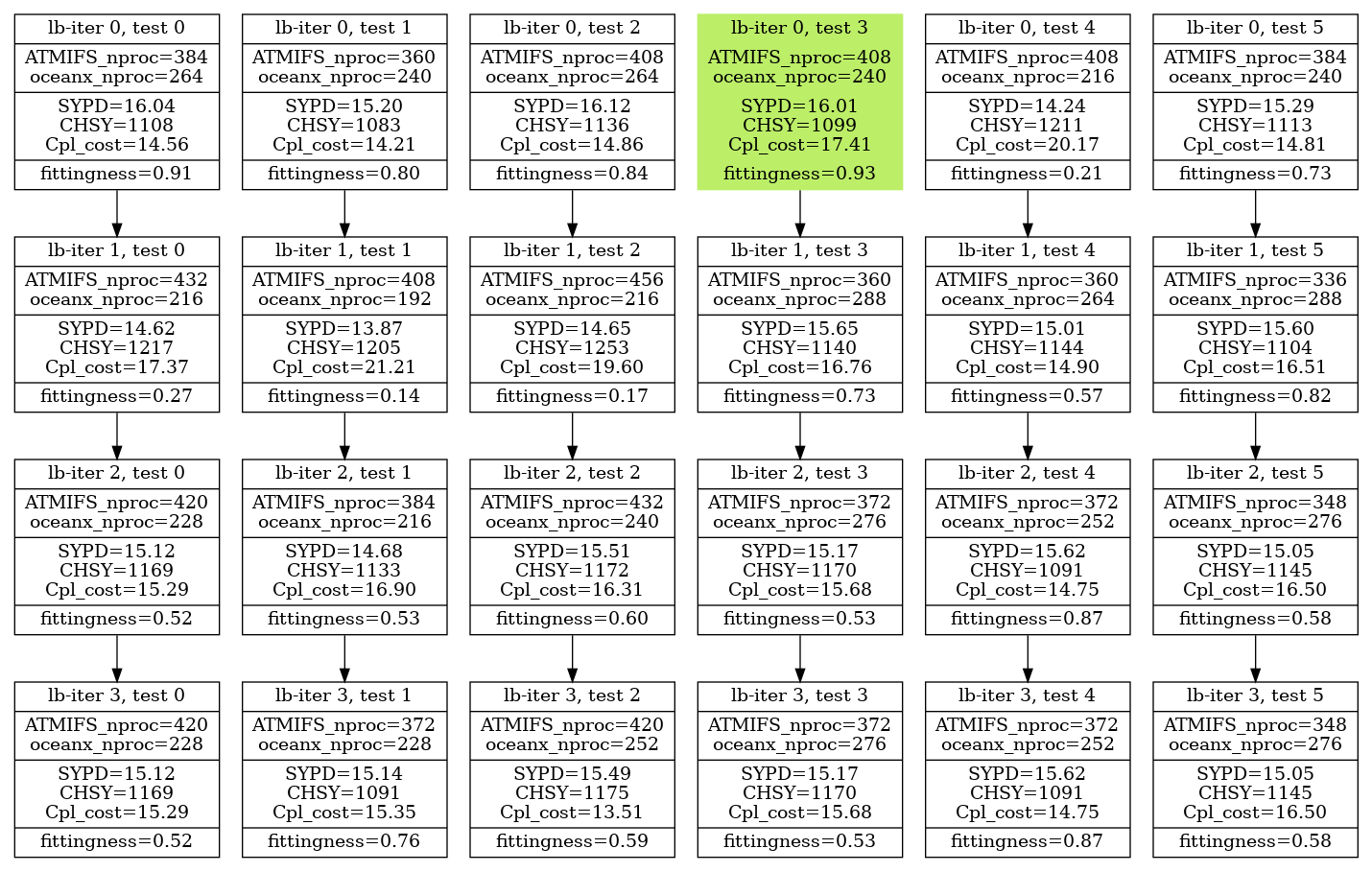
Figure 8 Performance results of each of the resource configurations tested to optimize an SR CMIP6 experiment. The metrics are the average of three runs of 6 months each.

5.2 EC-Earth3 at high resolution for the EUCP system

During the EUCP system project, a high-resolution experiment involving IFS and NEMO was used to simulate a total of 400 years. The configuration used for those experiments was 912 PEs for IFS and 1392 PEs for NEMO. Figure 9a shows the scalability of IFS. The CHSY does not increase much up to ∼ 500 processes, almost achieving an ideal speed-up. After 500 processes, some numbers of PEs seem to be better than others as the model SYPD curve is flat around 800, 900, and over 1000 PEs. Figure 9b shows the scalability of NEMO. We observe a superlinear speed-up as the CHSY is reduced as the number of PEs increases. The component, however, underperforms near 1000 PEs, and the execution cost starts increasing for configurations with the highest numbers of PEs.

Table 3 shows the default and the top five resource configurations found by the Prediction script plus the test with the original resource setup used before the analysis (orig). The max_nproc allowed was 2400, the TTS_w was set to 0.5. The load-balance workflow finishes after five iterations. The total execution time of the workflow is 50 h (1 HourPerTest × 2 TestsPerConfiguration × 5 InitialConfigurations × 5 lb-iterations = 50 h).

Figure 10 shows the results of the auto-lb workflow. The performance of the original resource configuration, shown in lb-iter 0, test 5, was 3.54 SYPD, 16 277 CHSY, and a coupling cost of 7.25 %. The best solution is found in lb-iter 4, test 4, and achieves a performance of 3.48 SYPD and 15 494 CHSY. This configuration is 1.7 % slower than the original but reduces the execution cost by 4.9 %. Moreover, note that also a new and better resource configuration was found while trying to reduce the coupling cost for the original one, lb-iter 3 test 5. This configuration uses 876 processes for IFS and 1428 for NEMO. The parallelization and the SYPD are the same as the original one but the CHSY is reduced by 363 (2.2 %).

Having used this experiment to simulate the 400 years, reducing the CHSY by 4.9 % is equivalent to saving the executing cost of running 400×4.9 % ≃ 20 years (and more than 300 000 core hours) with the same configuration.

Table 3 Top five initial configurations from the Prediction script to be used by the load-balance workflow to find a better resource configuration for the EUPC HR experiment using a TTS_w of 0.5.

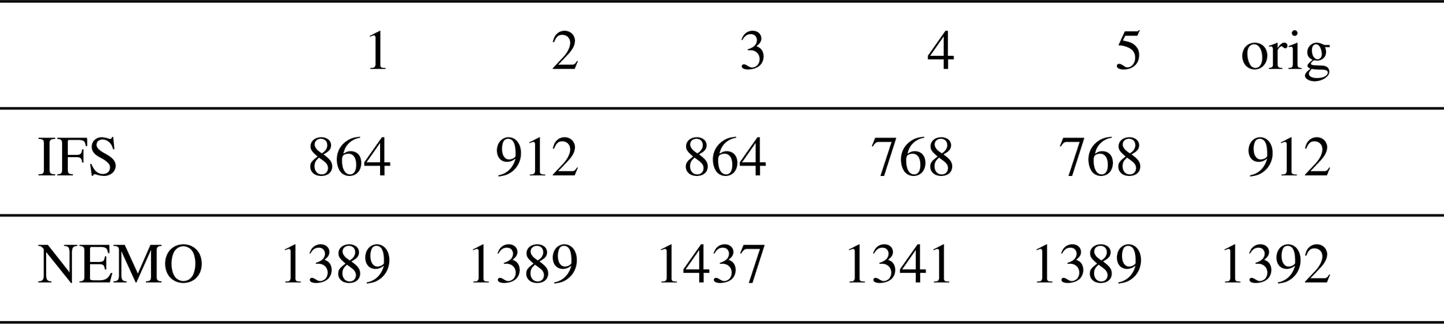
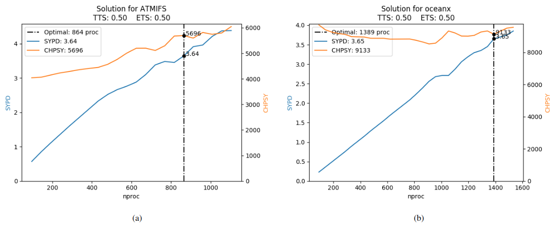
Figure 9 Scalability and predicted best PE allocation for IFS and NEMO at high resolution for an EUCP experiment using a TTS_w of 0.5.

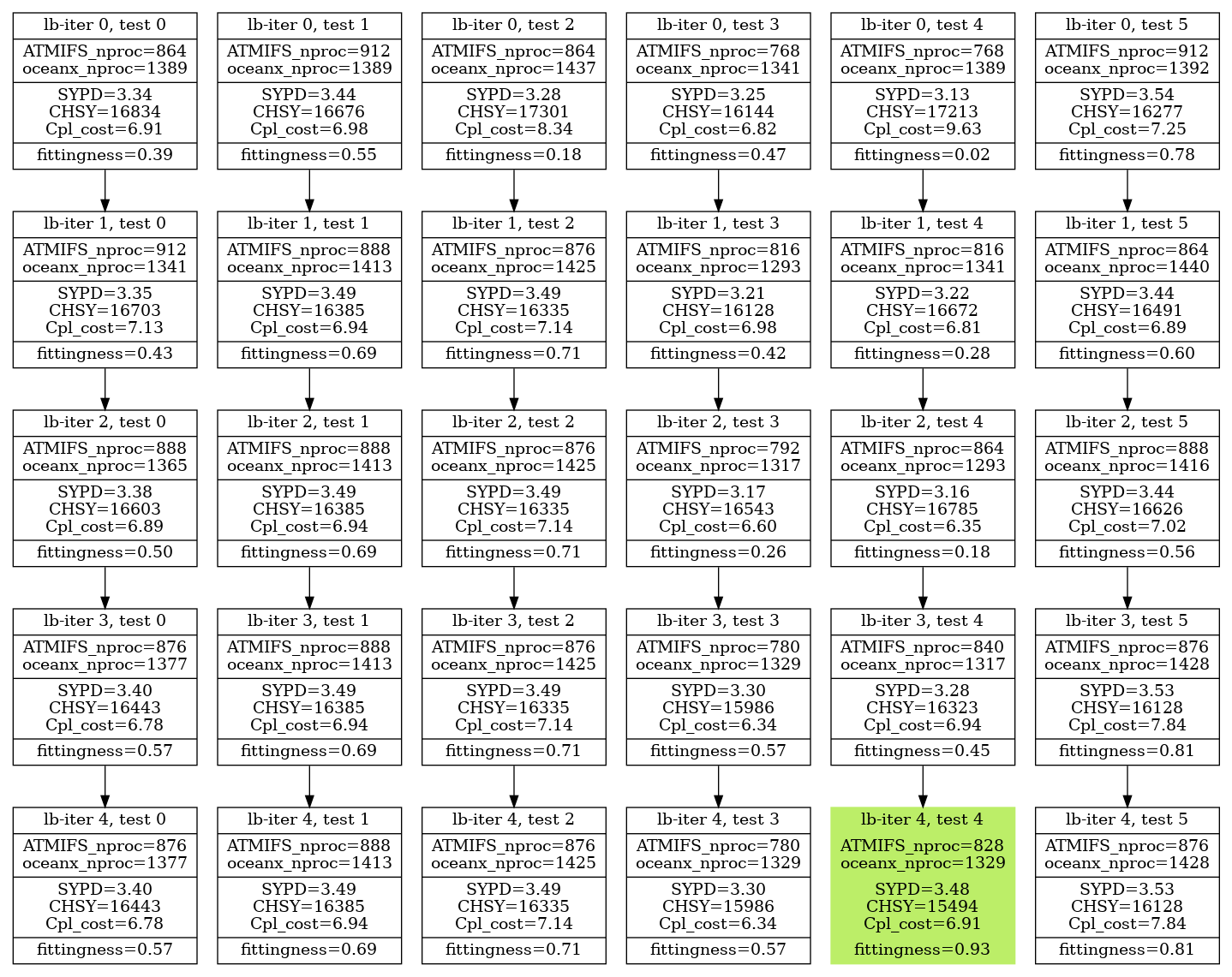
Figure 10 Performance results of each of the resource configurations tested to optimize a high-resolution European Climate Prediction Project (EUCP) experiment using a TTS_w of 0.5. The metrics represent the average of two runs of 2 months each.

5.3 Time-to-solution vs energy-to-solution

One of the novel features of auto-lb is the possibility of applying different performance/efficiency criteria depending on the context. This section demonstrates how using the TTS_w parameter can affect the outcome of the same experiment configuration.

Using the auto-lb workflow with a default TTS_w=0.5, we determined that the recommended setup for an EC-Earth3 experiment at standard resolution in the ECMWF machine (CCA HPC) is to use 684 PEs for IFS and 216 for NEMO. This configuration achieves 17.55 SYPD and consumes 1230 CHSY, with a coupling cost of 11.21 %.

However, due to constraints on the number of core hours allocated to the project on that machine, users require a more conservative setup that consumes fewer core hours. This can be easily achieved by rerunning the auto-lb workflow using a smaller TTS_w. For example, setting TTS_w=0.25 (ETS_w=0.75) provides a less costly configuration. Figure 11 presents the results of the workflow with TTS_w=0.25, starting from the following resource setups given by the Prediction script (IFS–NEMO): 576–144, 468–108, 432–108, 468–144, 540–144 (see lb-iter 0).

The best configuration is found in lb-iter 3 test 2, utilizing 423 PEs for IFS and 117 for NEMO. This configuration achieves 13.94 SYPD and 939 CHSY, with a coupling cost of 8.29 and using a total of 540 PEs. Compared to the solution found using TTS_w=0.5, this setup reduces the speed of the ESM by 25.9 % (17.55 vs 13.94), but improves the CHSY by 31 % (1230 vs 939). Furthermore, the coupling cost is reduced by $\mathrm{11.21}-\mathrm{8.29}=\mathrm{2.92}\mathit{\%}$ and fewer PEs are required to run. This can be visualized in Fig. 12, which shows the recommended parallelization for IFS (12a) and NEMO (12b) when changing TTS_w from 0.5 to 0.25.

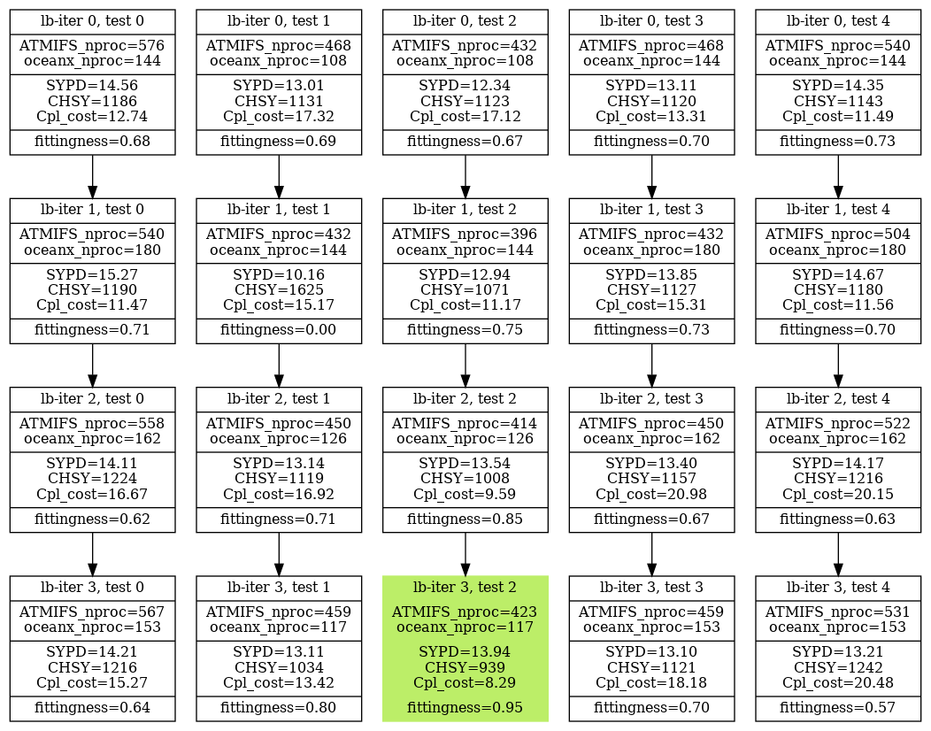
Figure 11 Performance results of each of the resource configurations tested to optimize a standard-resolution experiment of EC-Earth3 using a TTS_w of 0.25. The metrics are the average of three runs of 3 months.

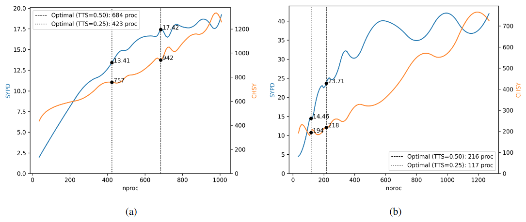
Figure 12 Scalability (SYPD and CHSY) and resource allocation for IFS (a) and NEMO (b) for an EC-Earth3 experiment at standard resolution on the ECMWF machine (CCA), using different time/energy criteria. For a TTS_w=0.50, the coupled run should utilize 684 PEs for IFS and 216 for NEMO. For a TTS_w=0.25, the coupled setup should be 423 PEs for IFS and 117 for NEMO.

6 Conclusions

Coupled earth system model (ESM) performance is limited by the load-balance between the constituents. While some works propose to deal with the problem by adapting the applications to support malleability, operational ESMs developed and maintained by different institutions in Europe mainly try to find the best resource configurations manually. Without an adequate methodology and an improved set of metrics for evaluating and addressing load imbalance, it has been demonstrated that coupled ESMs run with suboptimal resource configurations, leading to a diminishing of their speed and parallel efficiency.

This study introduces a novel methodology to improve resource allocation for each component in widely used EC-Earth3 experiments. The methodology includes a Prediction script to estimate the best possible solutions and an iterative process for running the simulations on a high-performance computer, collecting the performance metrics and making fine-grained optimizations to mitigate the coupling cost. The methodology has been integrated into the Barcelona Supercomputing Center (BSC) official workflow manager for EC-Earth3, Autosubmit, minimizing user intervention as much as possible. This integration allows any EC-Earth3 user using Autosubmit to easily take advantage of the auto-lb methodology on any of the other machines where the workflow manager is deployed (e.g., LUMI, MN5, MELUXINA, HPC2020). Additionally, auto-lb consists entirely of bash and Python scripts, making its core functionalities easily portable to other workflow managers or even runnable manually if required.

A new metric, fittingness, has been introduced to assess coupled ESM performance. It allows us to parameterize the energy/time trade-off. This flexibility enables the identification of multiple well-balanced solutions based on user-specific need, such as budget limitations for core hours and urgency in obtaining the output.

The results demonstrate the portability of the auto-lb method across various high-performance computing platforms, achieving improved resource configurations for different experiment configurations and resolutions. The authors believe that the best way to illustrate the usefulness of the proposed methodology is by showing its benefits for real and significant climate experiments that were carefully (manually) configured to maximize the performance. Therefore, Sect. 5.1 presents the computational improvements for a Coupled Model Intercomparison Project Phase 6 (CMIP6) experiment, which took months to simulate, covering over 14 000 years and consuming 15 million core hours on MareNostrum4 (Acosta et al., 2023a). The results suggest savings of 4.7 % of the execution time and a 1.3 % reduction in core hours needed. Similarly, Sect. 5.2 reports the results for a high-resolution EC-Earth3 experiment used in the European Climate Prediction (EUCP) project, simulating 400 years and consumed over 6.5 million core hours on MareNostrum4. With the new resource setup achieved using the auto-lb methodology, the core hours consumed could have been reduced by 4.9 % at the expense of increasing the execution time by 1.7 %. Alternatively, the method also provides another resource setup that maintains constant execution time but reduces the core hours required by 2.2 %. Finally, Sect. 5.3 presents two possible resource setups for EC-Earth3 on another HPC machine, European Centre for Medium-Range Weather Forecasts (ECMWF) CCA HPC. The two setups differ in the criteria used. For a more energy-efficient solution, the auto-lb methodology was used with a TTS_w=0.25 (ETS_w=0.75). This solution is 25.9 % slower than using the default value of TTS_w=0.50, but it reduces core hours by 31 % and uses fewer PEs, demonstrating that both solutions are viable and allowing the user to choose the most appropriate one depending on the specific context in which it will run.

Looking ahead, it is expected that ESMs will continue to grow in complexity, incorporating more components to simulate more features of the Earth system. For instance, some EC-Earth3 configurations already couple up to five different components simultaneously, resulting in a better representation of some Earth phenomena but increasing the load-imbalance significantly. Big upcoming international projects like the Coupled Model Intercomparison Project Phase 7 (CMIP7) are crucial for the advance of climate science, but they come at the expense of significant power consumption for computing. As shown, even with two-component systems, the solution space can easily grow into multiple hundreds of different resource setups. Adding more components exponentially increases this solution space, making the usage of manual tuning and traditional methods even more limited with future complex simulations. This underscores the necessity for developing more sophisticated tools like auto-lb.

At the same time, the increasing adoption of GPU acceleration in Earth system modeling software reflects a broader shift towards hybrid computing infrastructures. A good example of this trend can be found in the new EuroHPC systems, where seven out of eight integrate both CPU and GPU resources. Consequently, methodologies for load-balancing must evolve to account for these new hybrid architectures. While the principles described for the auto-lb approach remain relevant, heterogeneous CPU/GPU codes introduce additional complexities. The primary challenge lies in controlling the speed at which each component must run to maintain load balance. In a pure MPI setup, resource redistribution is straightforward as coupled components share a common pool of processing elements (PEs, physical cores) and can reallocate them while keeping the total amount of parallel resources used constant. In contrast, for components running on different hardware (e.g., CPUs and GPUs), the term “processing element” has different meanings, and resources are not directly interchangeable – a CPU core and a GPU core do not have a one-to-one equivalence. Extending the auto-lb methodology to hybrid CPU/GPU ESMs would require a standardized definition of computational resources. Such a definition could enable the optimization process to account for the equivalences and differences between CPUs and GPUs, potentially through an application-specific equivalent compute unit metric. This metric would involve profiling the performance characteristics of each component on both types of hardware to guide resource allocation decisions.

Moreover, it is important to highlight that some climate models include additional parallelization parameters that influence performance but have not been explicitly addressed in this manuscript. These include the ability to define different processor layouts (e.g., for 32 PEs, possible configurations could be 1×32, 2×16, 4×8) and the use of hybrid MPI/OpenMP parallelism. At present, these aspects are not managed within the auto-lb tool as we expect that this is already known before the balancing. It is important to emphasize that our methodology specifically addresses the load-balancing issues rather than optimizing the standalone performance of individual components. In cases where processor layouts or hybrid configurations must be considered, we first conduct an exploratory standalone performance analysis of each component to determine the most efficient processor layout and the optimal number of OpenMP threads per MPI rank. These parameters are then treated as fixed throughout the load-balancing process. If these cases become more readily available, it is possible to update the workflow for better handling.

To ensure efficient use of HPC resources, auto-lb functionality must be extended to support increasingly complex coupled configurations and models running on hybrid computing infrastructures. The combination of heuristics through a prediction script with the automatic iterative process (running the ESMs and collecting novel performance metrics) offers an efficient approach to finding better resource setups for coupled ESMs, while minimizing the time and core hours needed to find them.