Diagnosis of winter precipitation types using the spectral bin model (version 1DSBM-19M): comparison of five methods using ICE-POP 2018 field experiment data

Winter precipitation types (WPTs) are controlled by many factors, including thermodynamic and microphysical processes. Therefore, realistically simulating interactions between precipitation particles and the atmosphere is important when diagnosing the WPT. In the present study, we analyze the performance of a modified version of the one-dimensional spectral bin model (SBM; version 1DSBM-19M) of Carlin and Ryzhkov (2019), which simulates the change in the physical characteristics of precipitation particles of various sizes as they fall from the cloud top to the ground and diagnoses surface WPTs. We compare the performance of the SBM and four other diagnostic methods that use the following variables: (1) atmospheric thickness, (2) wet-bulb temperature, (3) temperature and relative humidity, and (4) wet-bulb temperature and low-level lapse rate. Three reference WPTs (snow (SN), rain (RA), and RASN) are obtained from particle size velocity (PARSIVEL) disdrometer data using a newly proposed decision tree algorithm. The results show that the SBM has the highest overall hit rate for all cases among five diagnostic methods. In contrast, the hit rate of the SBM for each WPT shows lower performance for RA than for the other methods. These results indicate that the SBM simulations tend to underestimate melting compared to observations. We thus explore the effects of the SBM's microphysics scheme on the extent of melting in cases of misdiagnosed RA. An optimized SBM that uses the climatological snow density–diameter relationship for the Pyeongchang region produces an increased amount of melting and achieves improved skill scores compared to the current SBM, which uses a snow density–diameter relationship for the Colorado region.

1 Introduction

There is a complex variety of winter precipitation types (WPTs), such as rain (RA), snow (SN), rain and snow (RASN), ice pellets (IPs), freezing rain (FZRA), and a mixture of ice pellets and freezing rain (IPFZRA). Various thermodynamical and microphysical processes can determine surface WPTs in nature. Some microphysical processes, such as melting, freezing, evaporation, and sublimation, change the phase and/or mass of precipitation particles and are diabatic thermodynamic processes. Other microphysical processes, such as riming and aggregation, modify particle size distributions (PSDs), habits, and the physical characteristics of individual particles such as their fall velocity and density (Heymsfield, 1972; Pruppacher and Klett, 1997; Libbrecht, 2001; Barthazy and Schefold, 2006; Lee et al., 2015; Gong et al., 2020; Vázquez-Martín et al., 2021). Aggregation widens PSDs by increasing the size of particles, while riming increases the terminal fall velocity and density of particles. Thus, the complexity of these processes should be accounted for when seeking to accurately diagnose WPTs.

Several simple empirical methods are commonly used to predict WPTs based on empirical relationships between specific meteorological variables and WPTs. For example, atmospheric thickness can be used to classify WPTs. Because atmospheric thickness is proportional to the mean virtual temperature (T_v) between two layers, a larger thickness is associated with a higher possibility of melting. Different thresholds for atmospheric thickness are used depending on the region under investigation (Koolwine, 1975; Stewart and King, 1987; Bluestein, 1993; Lee et al., 2014). In addition, nomograms of relative humidity (RH) and temperature (T) on the ground can be used to determine the WPT. Matsuo et al. (1981) proposed RH–T relationships to distinguish three WPTs (RA, RASN, and SN), and Lee et al. (2014) subsequently modified this using observational data. Wet-bulb temperature (T_w) can also be used as a predictor. T_w is defined as the temperature of the air when brought to saturation by the evaporation of water. T_w is a better-conserved quantity than T, which makes it useful for short-range predictions. Häggmark et al. (2000) developed a probability density function (PDF) for SN as a function of the surface T_w (T_w0). Recently, joint probability distributions for SN using T_w and Γ_low (low-level lapse rate; the rate of change in temperature from the surface to 500 m above ground level (a.g.l.), in °C km⁻¹) have been proposed based on an analysis of global statistical data (Sims and Liu, 2015). By including Γ_low, the scheme proposed by Sims and Liu (2015) takes into account situations where the melting of ice particles begins while they are falling, which is especially important for conditions that include low-level temperature inversions. However, because this scheme was developed using global data without regional and/or synoptic weather dependence, it is only valid when used in a globally averaged manner. The validity for the regions of this study has not been investigated in Sims and Liu (2015). In addition to those described here, many other WPT diagnostic methods based on the environment or numerical model data have been proposed (e.g., Ramer, 1993; Baldwin et al., 1994; Bourgouin, 2000; Schuur et al., 2012; Benjamin et al., 2016). As an example, Benjamin et al. (2016) suggested diagnostic logic for WPT using output of the Rapid Refresh (RAP) and High-Resolution Rapid Refresh (HRRR) models, such as 2 m T, total precipitation, precipitation except graupel, snow-only precipitation, snow fraction, and precipitation rate. The diagnostic logic classifies four WPTs (RA, SN, FZRA, IP) based on a decision tree method.

Other studies have attempted to predict WPTs using environmental data combined with an explicit microphysical model (e.g., Reeves et al., 2016). This approach is motivated by the fact that the rate of change between phases varies with particle size; for example, small particles may melt entirely, while larger particles remain predominantly ice. This subsequently affects refreezing because the threshold for T needed to initiate refreezing depends on whether an ice nucleus remains in the particle or whether it is entirely liquid. As such, the accurate diagnosis of WPTs at the surface requires consideration of these processes as a function of particle size, particularly for a mixture of WPTs (e.g., RASN and IPFZRA).

The one-dimensional spectral bin model (SBM) proposed by Reeves et al. (2016) separates the precipitation PSD into various bins and calculates the phase change for each of these bins at sequential height intervals using heat balance equations that depend on the environmental T and humidity (Rogers and Yau, 1989; Pruppacher and Klett, 1997). The resultant WPT (RA, SN, RASN, IP, FZRA, or IPFZRA) is predicted based on the relative fractions of ice and liquid at the surface (see Sect. 3.2 for more details). The original formulation (Reeves et al., 2016) used a fixed PSD of aggregated SN particles with various degrees of riming and was mass conserving by only considering melting and refreezing. Carlin and Ryzhkov (2019) expanded the microphysical component of the SBM to include varying PSDs, multiple particle habits, and sublimation and evaporation. The addition of sublimation and evaporation is motivated by the fact that these processes can effectively eliminate hydrometeor mass at the low end of the PSD, thus affecting the resulting classification. Evaluation of the original SBM optimized for the United States (Reeves et al., 2016) revealed that the model was highly skilled in discriminating FZRA and IPs but achieved slightly lower scores for SN and RA when compared to other algorithms that rely only on environmental metrics (Ramer, 1993; Baldwin et al., 1994; Bourgouin, 2000; Schuur et al., 2012). Owing to this continued development, there have been different versions of the SBM documented in the literature: the original version of Reeves et al. (2016), the so-called 1DSBM-19 described above (Carlin and Ryzhkov, 2019), and the new 1DSBM-19M presented herein (i.e., a modified version of 1DSBM-19). 1DSBM-19M is used in this study, with the differences from 1DSBM-19 described at https://doi.org/10.5281/zenodo.14350651 (Carlin et al., 2024).

Intensive observation networks employing a variety of instruments (e.g., disdrometers, weighing gauges, radar, lidar, and rawinsondes) were established at many sites along the South Korean coastline and across the Taebaek Mountains during the International Collaborative Experiments for Pyeongchang 2018 Olympic and Paralympic winter games (ICE-POP 2018) campaign (Lee and Kim, 2019; Gehring et al., 2020). The Taebaek Mountain ranges are complex, experiencing sudden changes in surface conditions due to the effects of the relatively warm ocean and cold mountainous terrain frequently occurring in this region. Thus, winter precipitation in this region is affected by different synoptic patterns, orographic effects, and air–sea interactions (Nam et al., 2014; Kim et al., 2019). There are also many local and small-scale phenomena to consider, such as the occurrence of cold pools due to the development of coastal fronts, the formation of inversion layers aloft as a result of these cool pools, and greater low-level thermal instability due to warm and moist advection from the ocean. Nevertheless, although the accurate diagnosis of the WPT is challenging in this region, the intensive observation data density available due to the ICE-POP network allows for an extensive evaluation and optimization of previously proposed WPT diagnosis methods.

In this study, we aim to compare the performance of the SBM (version 1DSBM-19M) with empirical methods in terms of diagnosing the WPT using observations from rawinsondes. The four empirical approaches tested are the 1000–850 hPa thickness (H₈₅₀ method), RH₀–T₀ method (Lee et al., 2014), T_w0 (Häggmark et al., 2000), and T_w0–Γ_low method (Sims and Liu, 2015). The diagnosed WPT is verified using WPT data obtained from particle size velocity (PARSIVEL) disdrometers collected during the ICE-POP 2018 period (November 2017–April 2018).

2 Data

2.1 ICE-POP 2018 observation sites

The northeastern region of South Korea is characterized by cold air and warm ocean temperatures in winter and complex, steeply sloped terrain from mountain ranges to the ocean (Fig. 1). An intensive observational survey was conducted in this region during the ICE-POP 2018 campaign from November 2017 to April 2018, with 20 PARSIVELs installed at 18 sites (the cross symbols in Fig. 1a) along the coastline and in the mountain ranges to record WPTs under various atmospheric conditions. Rawinsonde observations were also made every 3 h at five sites: two sites in the coastal region (Sokcho (SCW) and the Gangwon Weather Administration (GWW)), one site at the entrance of the mountain ranges (Bokwang1-ri Community Center (BKC)), and two sites in mountain valleys (Myeonon Observatory (MOO) and Daegwallyeong Regional Weather Office (DGW)). In addition, 11 micro rain radars (MRRs) were installed at some of the sites (square symbols in Fig. 1a). The MRRs are vertically pointing K-band radars, and their data are useful for understanding the vertical characteristics of precipitation.

The eastern sites in the Taebaek Mountains are at a relatively low altitude, with SCW, GWW, and BKC being 18, 79, and 175 m above mean sea level (a.m.s.l.), whereas the western sites (DGW and MOO) are 773 and 532 m a.m.s.l., respectively. We analyze the PARSIVEL data to identify the WPTs from the five sites (SCW, MOO, BKC, Gangneung-Wonju National University (GWU), and DGW; Fig. 1b–f) that are collocated with or closest to a rawinsonde observation. The PARSIVEL data at GWU are matched with sounding data from GWW, which is about 3.88 km away with a similar altitude (GWU: 36 m a.m.s.l.). This atmospheric environment and these high-resolution soundings are optimal for comprehensively testing the diagnosis of WPTs.

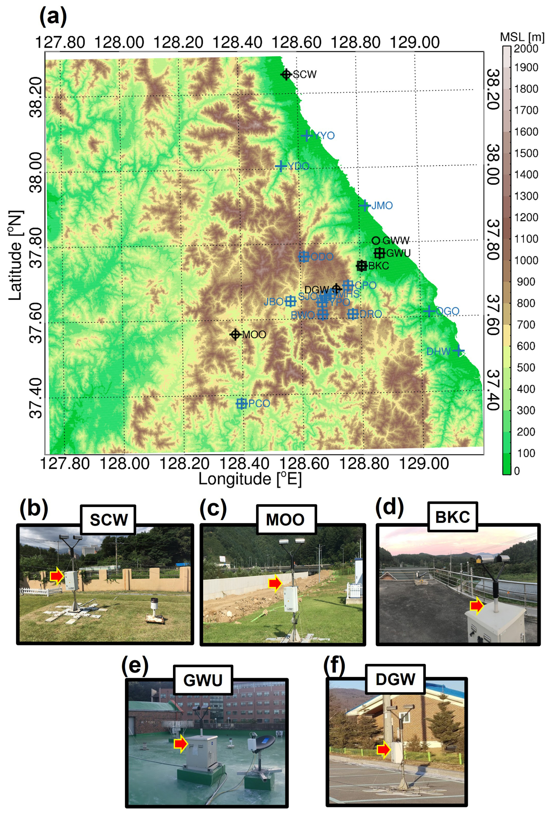
Figure 1 (a) Topography and observational supersites in the northeastern region of South Korea during the ICE-POP 2018 period. Photographs of PARSIVELs at the five sites: (b) SCW, (c) MOO, (d) BKC, (e) GWU, and (f) DGW. The cross symbols indicate PARSIVELs, and squares (circles) indicate MRRs (rawinsondes) in (a). The sites used in this study are labeled with text in (a).

2.2 Observational data and quality control

A PARSIVEL is a disdrometer that uses a laser beam with a wavelength of 780 nm to obtain a particle's equivolume diameter (D, mm) and terminal fall velocity (V_t, m s⁻¹) based on changes in the laser beam signals. The measurable range of D (V_t) is from 0.3 mm (0.1 m s⁻¹) to 30 mm (20 m s⁻¹). The overall error in D is within 5 %, and V_t has errors ranging from 10 % to 25 % as D changes (Löffler-Mang and Joss, 2000). We suggest how to deal with these measurement errors in Sect. 3.1. Version 2 PARSIVELs and level 1 data are used in the present study. Level 1 data are format-converted with no processing and provide particle counts for individual diameter and velocity channels (a 32 by 32 array) every minute. Because the observed PARSIVEL data contain outliers that may be the result of various forms of error, such as calibration errors and “margin fallers” (Yuter et al., 2006), we eliminate any of the level 1 data that meet at least one of the following two criteria: (i) D<1 mm and (ii) V_t>1.4V_a. V_a is the empirical relationship between D and V_t established by Atlas et al. (1973).

A modem-type rawinsonde (M10) is used for the ICE-POP 2018 campaign (In et al., 2018). The observation variables recorded by the M10 rawinsonde are pressure (P, hPa), T (°C), RH (%), wind speed (WS, m s⁻¹), and wind direction (WD, °) at 1 s intervals. Additionally, T_w is calculated using the two-parameter relationship for T and RH suggested by Stull (2011). Although rawinsonde data are useful as a reference of atmospheric vertical structure, the absolute accuracies of T and RH of the M10 rawinsonde sensor are 0.3 °C and 3 %, respectively (In et al., 2018). The impact of these measurement errors can be significant near 0 °C, where phase changes of precipitation particles occur.

The MRRs are modulated continuous-wave (FMCW) radars using a solid-state transmitter with a frequency of 24 GHz (Maahn and Kollias, 2012). In this study, the range resolution of the MRRs is set to 150 m. This resolution is enough to identify the melting layer (ML) because the average ML depth based on dual-polarization radar measurements from the Korean Peninsula during winter is about 670 m (Allabakash et al., 2019). MRR data include vertical profiles of radar reflectivity (Z, dBZ) and Doppler velocity (V_r, m s⁻¹) in precipitation. Z and V_r can be contaminated by noise, including non-meteorological echoes. Moreover, if V_r exceeds the Nyquist velocity boundaries (−6 to 6 m s⁻¹) of the MRR, aliasing of V_r will occur (Maahn and Kollias, 2012). In general, large raindrops in heavy-rainfall events cause the aliased data. Therefore, raw data from the MRRs are quality controlled using de-aliasing and the noise removal algorithm suggested by Maahn and Kollias (2012). The processed MRR data are used to provide additional context for important cases in the present study.

3 Methods

3.1 Determining the winter precipitation type

Three WPTs are considered in the present study: SN, RA, and RASN. SN is defined as solid precipitation such as dry snow, while RA is defined as liquid precipitation. FZRA is included in RA because it is in a liquid phase when observed by a PARSIVEL. RASN is mixed-phase precipitation that includes wet snow. IPs are very difficult to identify using only PARSIVEL data without photographic data because V_t of IP can have two modes: a low-speed mode that is similar to V_t of graupel or small hail and a high-speed mode similar to raindrops (Nagumo and Fujiyoshi, 2015). Thus, the lack of multi-angle snowflake cameras (MASCs) or similar equipment at some sites (DGW, SCW, and MOO) is an issue for this analysis. In addition, IPs in the Pyeongchang region are only observed under very specific atmospheric conditions (i.e., very strong inversion (>5 K) with a freezing layer at 800–900 hPa and melting layer (ML) at 700–800 hPa; Chae et al., 2024) and are thus rare.

The 5 min PARSIVEL data are projected onto a Yuter et al. (2006) scheme that divides the data into three regions (RA, SN, and an ambiguous region; Fig. 2a), after which the number (N) of particles for each type is counted. The fractions of F_RA and F_SN are calculated using the following equations:

$$\begin{array}{}\text{(1)}& \left\{\begin{array}{l}{F}_{\mathrm{RA}}=\mathrm{100}\left(\mathit{\%}\right)\times \frac{N_{\mathrm{RA}}}{N_{\mathrm{Total}}}\\ F_{\mathrm{SN}}=\mathrm{100}\left(\mathit{\%}\right)\times \frac{N_{\mathrm{SN}}}{N_{\mathrm{Total}}}\end{array}\right.,\end{array}$$

where N_RA and N_SN are the number of particles identified as raindrops and snow particles, respectively, and N_Total is the number of particles across all three regions.

We obtain a total of 131 matched precipitation cases to validate the five diagnostic methods during the ICE-POP period (1 November 2017–30 April 2018). If precipitation is observed when a sounding launches at a specific time and site, the event includes a matched precipitation case. Cases are identified that feature measurable precipitation at any of the five sounding sites that satisfy two conditions. We identify precipitation cases at each site that satisfies two conditions: (i) $N_{\mathrm{RA}}+N_{\mathrm{SN}}\ge \mathrm{15}$ within 5 min of the sounding start time, and (ii) −4 °C < T₀ < 6 °C and RH₀>40 % at the sounding start time. Here, T₀ and RH₀ are the data recorded 1 s after the start of the sounding that represent the surface T and RH measured by the rawinsonde. Based on this hydrometeor-type classification scheme, the dominant WPT of the matched precipitation cases is determined using the newly developed algorithm with the quality-controlled 5 min PARSIVEL data (Fig. 2b).

The newly developed algorithm consists of three steps: (i) an F_RA check, (ii) an F_SN check, and (iii) redetermination of the WPT. First, we classify RA from the matched precipitation cases while taking into account potential differences in the hardware calibration of each PARSIVEL. If the hardware is correctly calibrated, F_RA should be 100 % for pure rainfall cases. The normalized frequency (NF) distributions of F_RA during the ICE-POP period with a T_AWS of >7 °C are shown in Fig. 3. NF can be calculated as the frequency of each class divided by the total frequency. T_AWS is the 5 min mean temperature from the nearest automatic weather station (AWS), and F_RA is calculated using 5 min PARSIVEL data from the same site. The only exception is BKC, which has no corresponding AWS; in this case, F_RA from the PARSIVEL at BKC and T_AWS at GWU are matched, with T_AWS corrected for the difference in altitude between the two sites assuming a general temperature lapse rate (6.5 °C km⁻¹). The F_RA at which the cumulative NF (solid black line) reaches a threshold value of 0.05 is defined as F_site (dotted black line). F_site varies by site (GWU: 65.2 %, BKC: 81.1 %, SCW: 61.6 %, MOO: 57.9 %, and DGW: 68.1 %). Based on the information presented in Fig. 3, the matched precipitation cases at each site with F_RA>F_site are classified as RA.

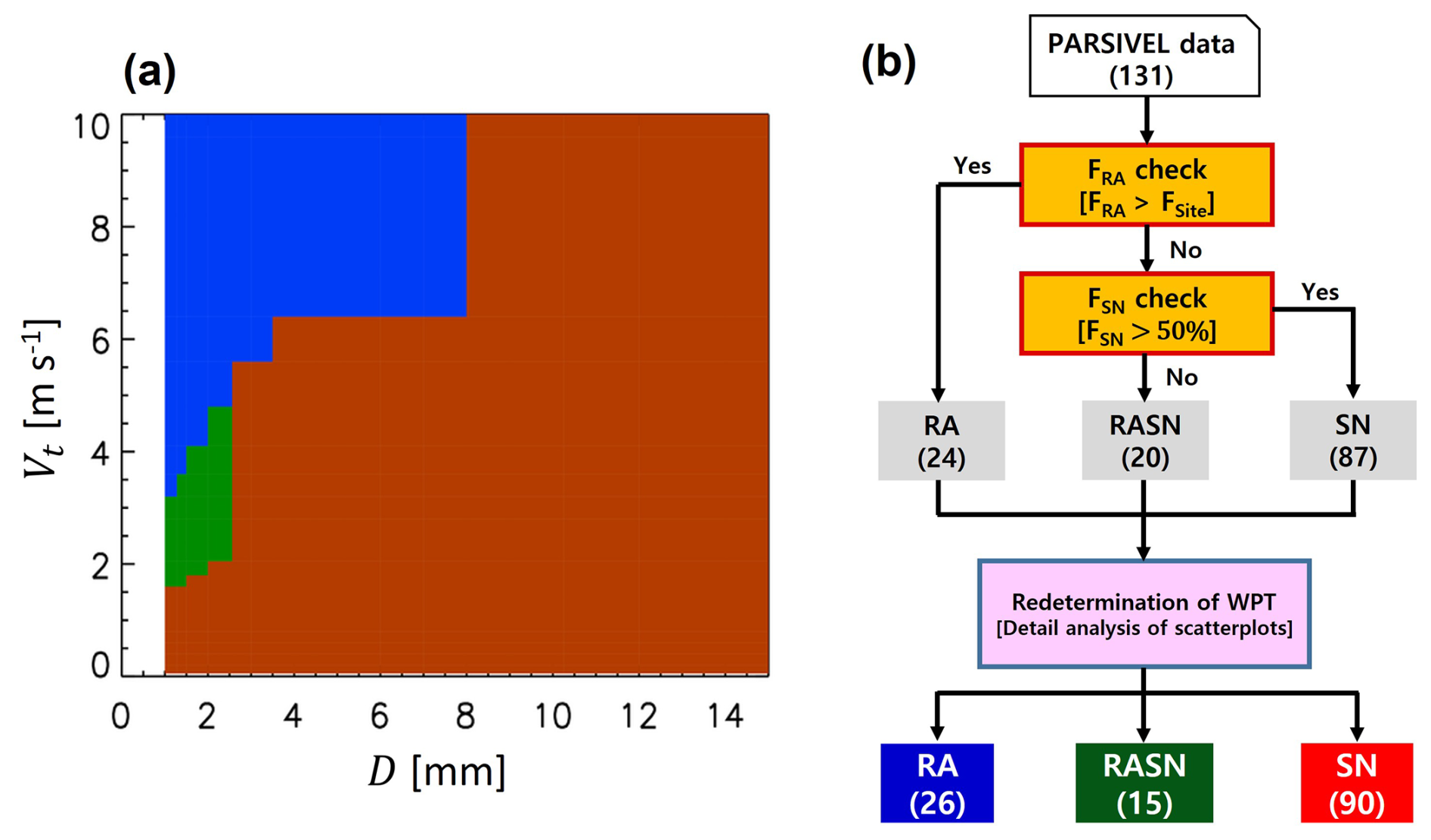
Figure 2 (a) Yuter et al. (2006) scheme. The color indicates the determined precipitation type, where blue (red) indicates RA (SN) and green indicates an ambiguous precipitation type. (b) A new decision tree algorithm of WPT from PARSIVEL data. The number of each WPT is shown in parentheses.

Second, we divide the remaining cases into high-SN-fraction (F_SN>50 %) and low-SN-fraction (F_SN≤50 %) groups. The high-SN-fraction group indicates a greater likelihood of dry snowfall and is classified as SN, while the low-SN-fraction group indicates a greater likelihood of wet snowfall and is classified as RASN. After these first two steps, the 131 matched precipitation cases are provisionally divided into 24 RA, 20 RASN, and 87 SN cases.

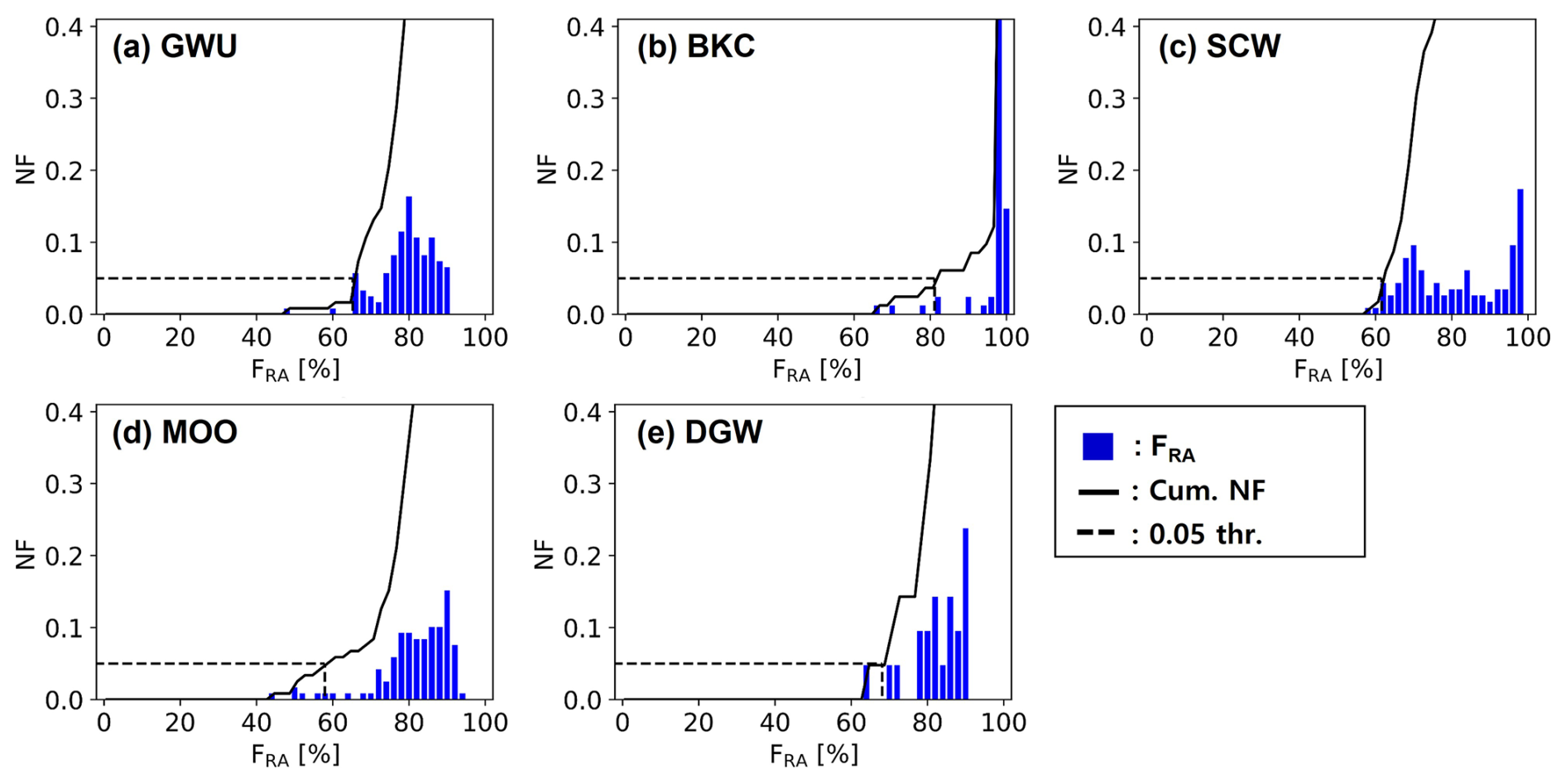
Figure 3 Normalized frequency distribution of F_RA of pure rainfall cases with T_AWS>7 °C during the ICE-POP period at (a) GWU, (b) BKC, (c) SCW, (d) MOO, and (e) DGW. The solid black line is cumulative NF, and the dotted black line is the 0.05 threshold.

In the third step, we manually examine the classification results using V_t–D scatterplots and redetermine the WPT of some cases that are clearly misclassified. Two RA cases and an SN case that have multiple curves in the V_t–D scatterplots are reclassified as RASN. Four RASN cases with a single curve similar to an empirical RA curve (Atlas et al., 1973) are reclassified as RA. Another four RASN cases with a single curve similar to an empirical graupel curve (Lee et al., 2015) are reclassified as SN. Two SN cases with a widely scattered distribution in their V_t–D scatterplot despite weak wind conditions (<3 m s⁻¹) at the near surface are reclassified as RASN. Two RASN cases with predominantly small snowflakes with various fall speeds are reclassified as SN because the cases are characterized by strong wind (≥9 m s⁻¹) near the surface and at low levels (<1 km a.g.l.), strong speed shear (≥5 m s⁻¹ km⁻¹), and very cold conditions (maximum T_w in sounding profile $\le -\mathrm{3}$ °C). Strong wind shear can lead to greater turbulence, thus generating tiny snowflakes (Dedekind et al., 2023) with chaotic movement that are more likely to be erroneously classified as RASN.

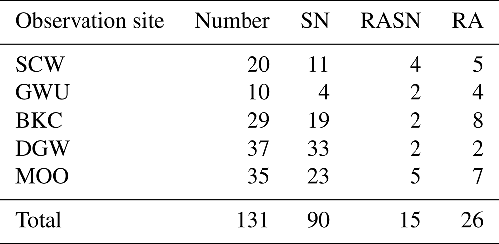
Following this redetermination step, a total of 26 RA, 15 RASN, and 90 SN cases are identified. The numbers of matched precipitation cases by observation site and WPT are listed in Table 1. More than half of the SN cases (56 of 90) occur at mountain sites (DGW and MOO), whereas many of the RA cases (17 of 26) occur at coastal sites (SCW, GWU, and BKC). A similar number of RASN cases occurs at both site types.

Table 1 The number of matched precipitation cases for each observation site and WPT.

3.2 Winter precipitation type diagnosis methods

The efficacy of the SBM and four empirical methods for diagnosing WPT is evaluated using the observed sounding data. Nomograms for the WPT for each of the four empirical methods are presented in Fig. 4. H₈₅₀ diagnoses the WPT based on a threshold 1000–850 hPa thickness that is empirically determined (Fig. 4a; Lee et al., 2014). H₈₅₀ is calculated as follows:

$$\begin{array}{}\text{(2)}& {\displaystyle }{H}_{\mathrm{850}}={\displaystyle \frac{R_{\mathrm{d}}\stackrel{\mathrm{‾}}{T_{\mathrm{v}}}}{g}}\ln {\displaystyle \frac{P_{\mathrm{1}}}{P_{\mathrm{2}}}},\text{(3)}& {\displaystyle }\left\{\begin{array}{l}\text{RA:}{H}_{\mathrm{850}}\ge {\mathrm{H}}_{\mathrm{RA}}\\ \text{SN:}{H}_{\mathrm{850}}<{\mathrm{H}}_{\mathrm{SN}}\\ \text{RASN:}{H}_{\mathrm{SN}}\le H_{\mathrm{850}}<H_{\mathrm{RA}},\end{array}\right.\end{array}$$

where R_d is the dry-air constant (287 J K⁻¹ kg⁻¹), g is the standard gravitational acceleration (m s⁻²), P₁ is 1000 hPa, P₂ is 850 hPa, and $\stackrel{\mathrm{‾}}{T_{\mathrm{v}}}$ is the mean T_v between 850 and 1000 hPa. T_v is calculated as a function of T, P, and RH (Lin, 2016). When the 1000 hPa data are unavailable, such as at the high-altitude sites (DGW and MOO), we use T_v at 925 hPa as an alternative for $\stackrel{\mathrm{‾}}{T_{\mathrm{v}}}$. The diagnosed WPT is SN if H₈₅₀ is lower than H_SN, while it is RA if H₈₅₀ is higher than H_RA. When H₈₅₀ is between H_SN and H_RA, the diagnosed WPT is RASN. Lee et al. (2014) determined that the H_SN and H_RA of South Korea at low-altitude sites (<100 m a.m.s.l.) are 1281 and 1297 gpm, respectively, whereas the H_SN and H_RA of DGW are 1299 and 1313 gpm, respectively. The WPTs at GWU, BKC, and SCW are diagnosed using the former critical values, while DGW and MOO are diagnosed using the latter. The reason for using different critical values is that GWU, BKC, and SCW are located near the East Sea at a low altitude and east of the Taebaek Mountains, whereas DGW and MOO are located within the Taebaek Mountains and are situated at a relatively higher altitude (Fig. 1a).

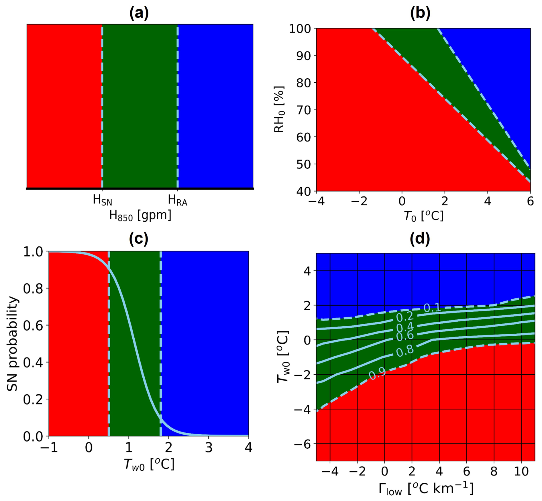
Figure 4 Nomograms for diagnosis of WPTs. The different colors indicate SN (red), RASN (green), and RA (blue). Classification of WPTs using (a) H₈₅₀ and (b) the RH₀–T₀ graph is shown with the dashed lines suggested in Lee et al. (2014). (c) Probability function (solid line) of SN as a function of the wet-bulb temperature at the surface, T_w0 (Häggmark and Ivarsson, 1997). (d) Probability distribution (solid and dashed lines) of SN on the T_w0–Γ_low graph for land areas (Sims and Liu, 2015). Here, the subscript “0” indicate the near-surface value.

The RH₀–T₀ method employs the shifted Matsuo scheme suggested by Lee et al. (2014). Figure 4b presents the diagnosed WPTs based on the RH₀–T₀ plot, with the two dashed lines derived from the following equations (Lee et al., 2014):

$$\begin{array}{}\text{(4)}& {\displaystyle }{\mathrm{RH}}_{\mathrm{0}}=-\mathrm{12}{T}_{\mathrm{0}}+\mathrm{120},\text{(5)}& {\displaystyle }{\mathrm{RH}}_{\mathrm{0}}=-{\displaystyle \frac{\mathrm{100}}{\mathrm{13}}}{T}_{\mathrm{0}}+\mathrm{89.5},\end{array}$$

where T₀ and RH₀ are in degrees Celsius and percentage, respectively. Equations (4) and (5) are used to separate RA from RASN and RASN from SN, respectively.

Third, the T_w0 method uses the probability of SN as a function of T_w0 to diagnose WPT (Fig. 4c, Häggmark et al., 2000). We used threshold probability values of 10 % and 90 % for the classification of WPTs. Thus, the diagnosed WPT is SN if the wet-bulb temperature at the surface (T_w0) is lower than 0.5 °C, whereas it is classified as RA if T_w0 is larger than 1.8 °C. When 0.5 °C ≤ T_w0 < 1.8 °C, the diagnosed WPT is RASN. Other probability values (20 % and 80 %; 30 % and 70 %) are also explored.

Using global surface-based (land station and shipboard) observations over multiple decades, Sims and Liu (2015) studied the influence of various geophysical parameters on precipitation phase, including near-surface air T, atmospheric moisture, low-level vertical T lapse rate (Γ_low), surface skin temperature, surface pressure, and land cover type. Because snow melting occurs close to T_w (∼ 0 °C) instead of the actual air T, Sims and Liu (2015) evaluated the SN–RA transition using T_w instead of air T. Their analysis indicated that, in addition to T_w, the vertical T lapse rate between the surface and 500 m significantly affects the precipitation phase. For example, at a near-surface T_w of 0 °C, a lapse rate of 4 °C km⁻¹ results in a conditional probability of 0.814 for solid precipitation, while a lapse rate of −3 °C km⁻¹ (inversion) results in a probability of 0.404 (Fig. 4d: conditional probability of solid precipitation on land). Based on this finding, they developed a WPT diagnostic scheme that employs T_w and Γ_low as inputs and returns the conditional probability of solid precipitation. The conditional probability was derived by the ratio of the number of solid precipitation cases divided by the number of any precipitation cases under the prescribed T_w and Γ_low conditions. This algorithm has been incorporated into the current Global Precipitation Measurement (GPM) mission algorithm used to determine precipitation phases (Huffman et al., 2020). Because the probability is computed using global data without accounting for regional and/or synoptic weather dependencies, its performance over the ICE-POP 2018 domain has not been examined. Similar to the previous method, threshold probabilities of 0.1 and 0.9 are used to classify the WPT using the T_w0–Γ_low method (Fig. 4d), though other threshold values (0.2 and 0.8; 0.3 and 0.7) are also explored. Γ_low is defined as

$$\begin{array}{}\text{(6)}& {\mathrm{\Gamma }}_{\mathrm{low}}={\displaystyle \frac{(T_{\mathrm{0}\mathrm{m}\mathrm{a}.\mathrm{g}.\mathrm{l}.}-T_{\mathrm{500}\mathrm{m}\mathrm{a}.\mathrm{g}.\mathrm{l}.})}{\mathrm{0.5}\mathrm{km}}}.\end{array}$$

As described in Sect. 1, the SBM simulates the characteristics of precipitation particles across the size spectrum as they fall through the ambient environment. Figure 5a presents the general process used by the SBM. When initialized from an external sounding (as done in this study), the cloud top is denoted as the highest height with an RH of at least 80 % (Reeves et al., 2016). From the cloud top to the surface, environmental variables are then calculated and interpolated to a 10 m vertical grid spacing. Because the particle bins are independent (i.e., no aggregation/breakup is accounted for), the SBM loops through each height level for a given particle size bin before considering the next larger size. Sublimation occurs in environments subsaturated with respect to ice if the particles have no meltwater; if the particles do contain meltwater, evaporation occurs if the environment is subsaturated with respect to water. Similarly, melting occurs if there is ice mass remaining and the surface T of the particle reaches 0 °C. Refreezing occurs under two conditions: if there is both liquid and ice present in a particle and T_w is below 0 °C or if T_w is at or below the nucleation T (T_c, °C) regardless of the remaining ice mass because re-nucleation is assumed to occur. Each microphysical process results in temporal trends in the ice and/or water mass, which is used to calculate the total change in ice or water mass within a given grid level based on the particle residence time. After this, all of the particle properties (e.g., density and terminal fall velocity) are updated to reflect the new mass and composition of each particle, and these serve as the initial particle properties for the subsequent grid level. This process continues until the bin is empty (i.e., the entire particle mass has sublimated or evaporated) or until the surface is reached. For more details, see Reeves et al. (2016) and Carlin and Ryzhkov (2019).

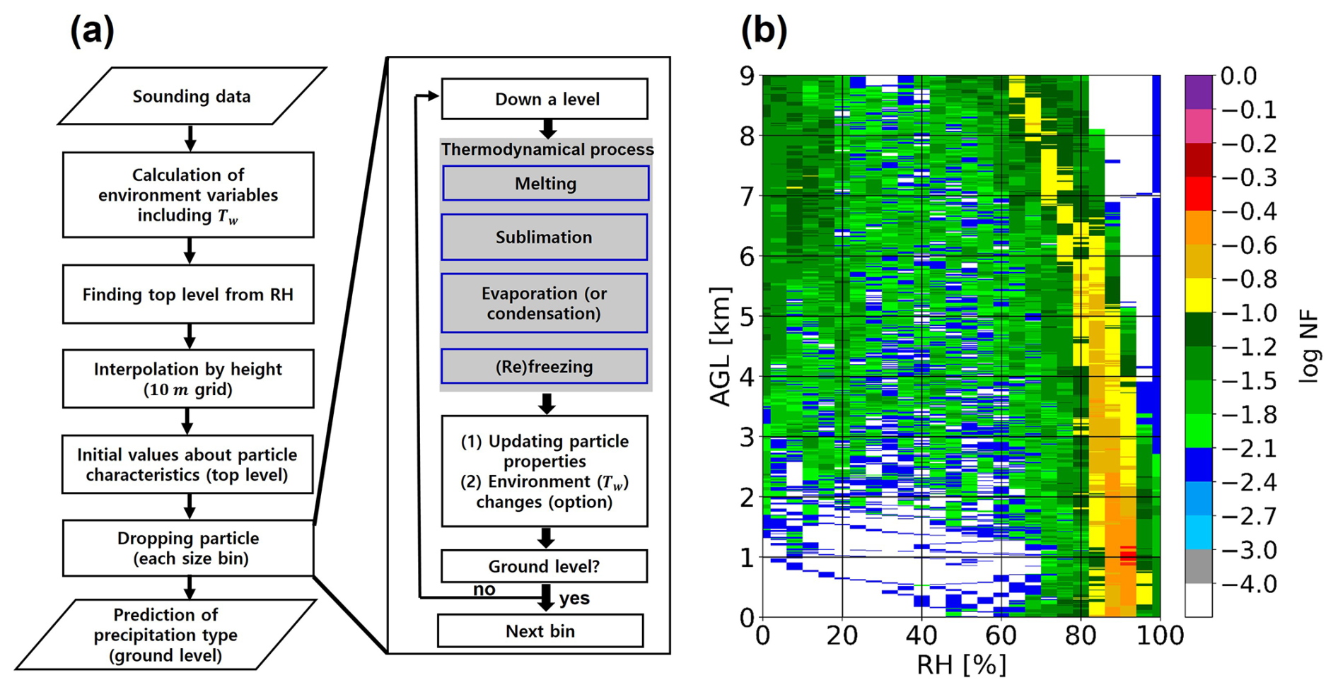
Figure 5 (a) Flowchart describing the SBM structure (adapted from Reeves et al., 2016; Carlin and Ryzhkov, 2019). (b) Contoured frequency by altitude diagram (CFAD) of RH from rawinsonde data for the 131 matched precipitation cases.

Once all of the particle characteristics at the ground level have been calculated, an overall WPT classification is determined based on the rainfall rate (R; mm h⁻¹) and snowfall rate (SR; mm h⁻¹) calculated from the ground PSD. The WPT logic of 1DSBM-19 considers the relative fractions of R and SR, the cloud top T (to determine whether ice nucleation occurs), the number of times the T_w profile crosses 0 °C, and the surface T_w (Reeves et al., 2016) to determine which of the six WPTs is dominant. However, in the present study, we are primarily interested in RA, SN, and RASN only. Therefore, we simplify the classification scheme of 1DSBM-19 as follows:

$$\begin{array}{}\text{(7)}& \left\{\begin{array}{l}\text{RA:}R>\mathrm{0}\mathrm{mm}{\mathrm{h}}^{-\mathrm{1}}\mathrm{and}\mathrm{SR}=\mathrm{0}\mathrm{mm}{\mathrm{h}}^{-\mathrm{1}}\\ \text{SN:}R=\mathrm{0}\mathrm{mm}{\mathrm{h}}^{-\mathrm{1}}\mathrm{and}\mathrm{SR}>\mathrm{0}\mathrm{mm}{\mathrm{h}}^{-\mathrm{1}}\\ \text{RASN:}R>\mathrm{0}\mathrm{mm}{\mathrm{h}}^{-\mathrm{1}}\mathrm{and}\mathrm{SR}>\mathrm{0}\mathrm{mm}{\mathrm{h}}^{-\mathrm{1}}.\end{array}\right.\end{array}$$

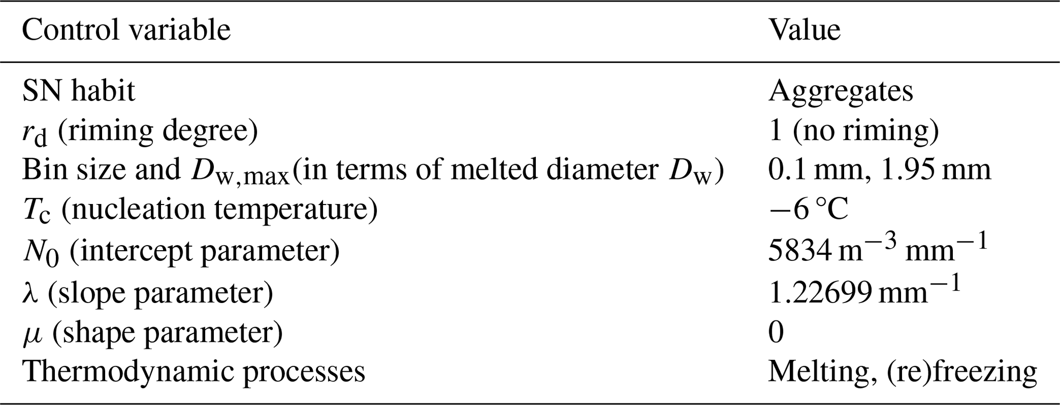
The SBM parameters used in this study are presented in Table 2. The particles are separated into 20 size bins and initialized as “unrimed low-density snow aggregates” because there are only 13 graupel-like events among the 91 SN events following the hydrometeor classification method suggested by Lee et al. (2015). The size bins are delineated such that the equivolume diameters of fully melted particles of equal mass in each bin are 0.1 mm apart. The largest size bin used in this study, with a fully melted equivolume diameter D_mw,max of 1.95 mm, is about 2 times the mean value of the mass-weighted mean diameter (∼ 1 mm) obtained from long-term rainfall observations in South Korea (Bang et al., 2020; Kwon et al., 2020). T_c is set to −6 °C following Reeves et al. (2016). The initial PSDs are assumed to be inverse exponential (μ=0) and are obtained through a statistical analysis of PARSIVEL data in the Pyeongchang region (Bang et al., 2019). The average values of N₀ and λ (Table 2) are taken from the averages of the leeward and windward sites examined by Bang et al. (2019). Because the PSDs used to initialize the model are measured at the surface, we assume no mass growth/loss from the particles (e.g., evaporation/sublimation) for simplicity and instead only consider melting/refreezing. The assumption of mass conservation should generally be valid for this study because almost all of the precipitation cases are nearly saturated (RH > 80 %) below 5 km a.g.l. (Fig. 5b). The initial PSD is fixed for all events because of the lack of aircraft microphysical observation data and the exclusion of explicit aggregation/riming processes in the microphysics scheme in the current SBM.

Table 2 Parameters for the SBM simulation used in this study.

3.3 Evaluation methods

We evaluate the performance of the five different methods against the observed WPTs described in Sect. 3.1. We quantitatively evaluate the methods using the hit rate (h, %) and modified hit rate (h^′, %) as the skill scores:

$$\begin{array}{}\text{(8)}& {\displaystyle }h={\displaystyle \frac{E}{O}}\times \mathrm{100}\mathit{\%},\text{(9)}& {\displaystyle }{h}^{\prime }={\displaystyle \frac{\mathrm{1}}{\mathrm{3}}}(h_{\mathrm{SN}}+h_{\mathrm{RASN}}+h_{\mathrm{RA}})\times \mathrm{100}\mathit{\%},\end{array}$$

where O is the number of observed cases, and E is the number of correctly diagnosed cases among the observed cases for each method. We calculate h, h_SN, h_RASN, h_RA, and h^′ for each of the diagnosis methods. Here, h without a subscript is the overall hit rate, h with a subscript (SN, RASN, RA) represents the accuracy for each WPT type, and h^′ is the average accuracy across all three WPTs. Additionally, skill scores that consider false alarms (F) are also calculated:

$$\begin{array}{}\text{(10)}& {\displaystyle }\mathrm{CSI}={\displaystyle \frac{E}{O+F}},\text{(11)}& {\displaystyle }\mathrm{FAR}={\displaystyle \frac{F}{E+F}},\end{array}$$

where CSI is the critical success index, and FAR is the false alarm rate (Shin et al., 2022). The skill scores are also compared between the mountain sites (DGW and MOO) and coastal sites (GWU, SCW, and BKC), and the effect of vertical T_w profiles on the accuracy of each diagnosis method is investigated to assess the strengths and weaknesses of each diagnosis method.

We also evaluate the microphysics scheme in the SBM by analyzing cases that are misdiagnosed by the SBM. Misdiagnosis of precipitation in the Pyeongchang region may occur due to regional differences in microphysical precipitation characteristics. In particular, the current SBM uses a snow density–diameter relationship obtained from two-dimensional video disdrometer (2DVD) data in Colorado (${\mathit{\rho }}_s=\mathrm{0.178}{D}^{-\mathrm{0.922}}$; Brandes et al., 2007).

A region-specific density–diameter relationship is derived from 2DVD measurements at DGW (collected by Lee et al., 2015) to reflect the microphysical characteristics of snow in this region. A power-law-based regression is performed using the weighted total least squares (WTLS) method (Amemiya, 1997) to minimize the deviation from both the x and the y axes (Lee et al., 2015). The region-specific density–diameter relationship for this dataset that includes dendrites, plates, and needles is derived as follows:

$$\begin{array}{}\text{(12)}& {\mathit{\rho }}_{\mathrm{s}}=\mathrm{0.09}{D}^{-\mathrm{1.01}}.\end{array}$$

In this relationship, the density of snow particles in this region is generally lower than that of Brandes et al. (2007), though with a similar inverse relationship between the diameter and density. Using this relationship to optimize the microphysical scheme of the SBM, we investigate the performance of the optimized model for the misdiagnosed cases.

4 Results

4.1 Overall accuracy of the diagnosed precipitation types

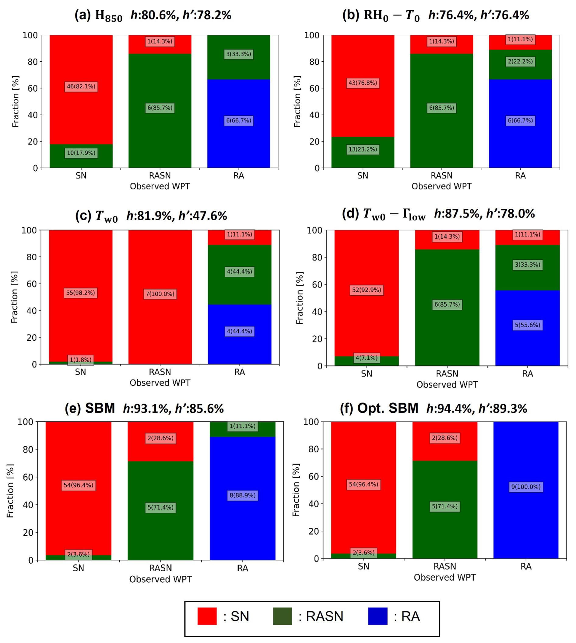
We evaluate the performance of the H₈₅₀ method, the RH₀–T₀ method, the T_w0 method with 10 % and 90 % probability values, the T_w0–Γ_low method with 0.1 and 0.9 threshold values, the current SBM, and the optimized SBM (Fig. 6a–f, respectively) in terms of diagnosing the WPT of the matched precipitation cases. Overall, the optimized SBM produces the highest h (93.1 %) and h^′ (87.5 %). The lowest h is from the RH₀–T₀ method (71.8 %), while the lowest h^′ is exhibited by the T_w0 method (68.4 %). The H₈₅₀ method (h: 72.5 %, h^′: 77.5 %) and the RH₀–T₀ method (h: 71.8 %, h^′: 78.0 %) have similar skill scores. The skill score sensitivity of the T_w0 and T_w0–Γ_low methods is analyzed according to probability values (or threshold values). The skill scores of the T_w0 method with 20 % and 80 % probability values are h=86.3 % and $h^{\prime }=\mathrm{66.6}$ % compared to h=86.3 % and $h^{\prime }=\mathrm{63.7}$ % for probability values of 30 % and 70 % (data not shown), which are lower than those for the default 10 % and 90 % thresholds (Fig. 6c). In addition, the skill scores of the T_w0–Γ_low method with 0.2 and 0.8 threshold values are h=88.5 % and $h^{\prime }=\mathrm{78.8}$ %, while those for 0.3 and 0.7 threshold values are h=90.8 % and $h^{\prime }=\mathrm{77.1}$ % (data not shown). The T_w0–Γ_low method with 0.1 and 0.9 threshold values has a lower h (85.5 %) and a higher h^′ (85.6 %) (Fig. 6d).

Although the H₈₅₀ and RH₀–T₀ methods are optimized for the Korea region, their h and h^′ are lower than those of the SBM and T_w0–Γ_low method. The T_w0 method exhibits a relatively large difference between h (86.3 %) and h^′ (68.4 %), with the inclusion of T_w0 improving the diagnosis of SN because the accuracy of SN for methods that include T_w0 (Fig. 6c and d) is much higher than for those that do not include T_w0 (Fig. 6a, b). Although the T_w0 method has the highest h_SN (98.9 %), a significant number of RASN events are misdiagnosed as SN (h_RASN: 33.3 %). Because the 90 % conditional probability of SN for land areas varies from $T_{\mathrm{w}\mathrm{0}}=-\mathrm{0.1}$ °C at Γ_low=11 °C km⁻¹ to $T_{\mathrm{w}\mathrm{0}}=-\mathrm{4.1}$ °C at ${\mathrm{\Gamma }}_{\mathrm{low}}=-\mathrm{5}$ °C km⁻¹ (Sims and Liu, 2015, Fig. 4d), T_w0=0.5 °C is too warm for the threshold. The T_w0–Γ_low method approach has a higher accuracy for the diagnosis of RASN cases and lower accuracy for SN cases compared to the SBM. However, h_RA is relatively low for the SBM (h: 69.2 %), with 8 of the 26 RA cases diagnosed as RASN, suggesting that the amount of melting differed between the simulations and the actual event. The diagnosis accuracy for the RA cases improves when using the optimized SBM by about 15 %, while the accuracy for the other WPTs does not differ between the current and optimized SBMs.

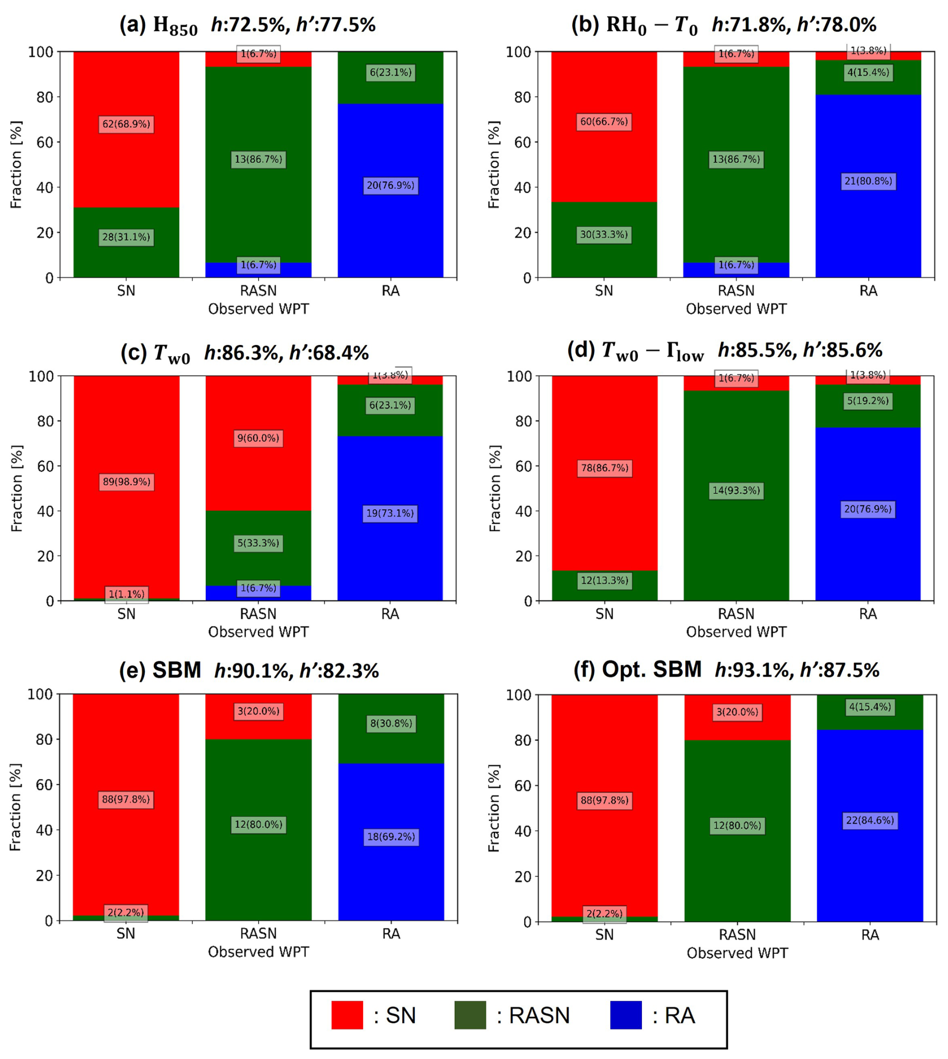
Figure 6 Evaluation summary of the five diagnosis methods for 131 matched precipitation cases (all cases). The methods are (a) the thickness method H₈₅₀, (b) shifted Matsuo scheme using an RH₀–T₀ method, (c) the wet-bulb temperature method T_w0, (d) the Sims and Liu scheme using the T_w0–Γ_low method, (e) the current SBM, and (f) the optimized SBM. The x axis is the observed precipitation type, and the colors indicate the fraction of the diagnosed precipitation types: red, SN; green, RASN; and blue, RA. The diagnosed fraction of precipitation types is shown on the y axis, with the number of cases labeled in each bar. The hit rate (h) and modified hit rate (h^′) are shown as the numbers on the top of each image.

Figure 7 Same as in Fig. 6 but for the 72 mountain cases.

The matched precipitation cases are divided into mountain sites (DGW and MOO) and coastal sites (GWU, BKC, and SCW), with the skill scores presented in Figs. 7 and 8, respectively. For the mountain sites, h (94.4 %) and h^′ (89.3 %) are the highest for the optimized SBM (94.4 % and 89.3 %, respectively), and the lowest values are observed with the RH₀–T₀ method approach (h: 76.4 %) and the T_w0 method (h^′: 47.6 %; h_RASN: 0 %). For the coastal sites, the T_w0 method and the optimized SBM (h: 91.5 %) and the T_w0–Γ_low method (h^′: 88.2 %) exhibit the highest accuracy; in contrast, H₈₅₀ produces the lowest accuracy (h: 62.7 %, h^′: 72.3 %, h_SN: 47.1 %). The skill scores for the T_w0 method at the mountain sites are lower than those at the coastal sites, whereas the opposite is true for the H₈₅₀ method and the RH₀–T₀ method approach. The T_w0 method exhibits significant differences in both h_RASN and h_RA with terrain, with coastal site scores exceeding those of mountain sites. The H₈₅₀ and RH₀–T₀ methods exhibit large differences in h_SN with changes in the terrain, with the mountain sites scoring higher than the coastal sites. In contrast, the skill scores for the SBM are higher at the mountain sites compared to at the coastal sites, while the skill scores for the optimized SBM with RA cases are higher than those for the current SBM at both mountain sites and coastal sites. The h value of the T_w0–Γ_low method at the mountain sites is higher than the h value at the coastal sites, while h^′ is lower. The T_w0–Γ_low method and the SBM exhibit considerable differences in h_RA, with the T_w0–Γ_low method producing a lower h_RA at the mountain sites than at the coastal sites and the SBM demonstrating the opposite.

Figure 8 Same as in Fig. 6 but for the 59 coastal cases.

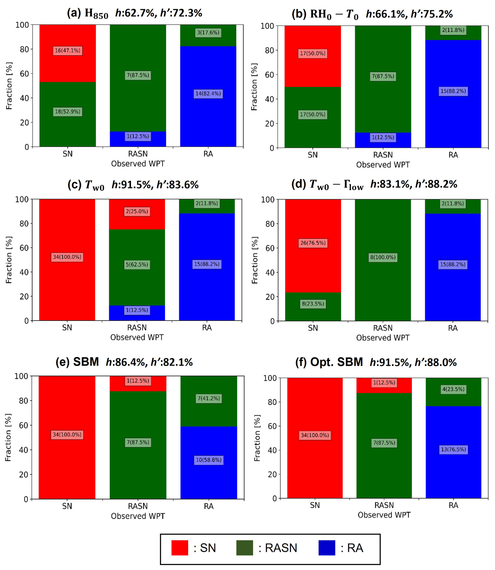
Table 3 CSI of the five diagnosis methods, indicated as event category. The bolded (italic) values denote the best (worst) performance among the five diagnosis methods within each event category.

Table 4 As in Table 3 but for FAR.

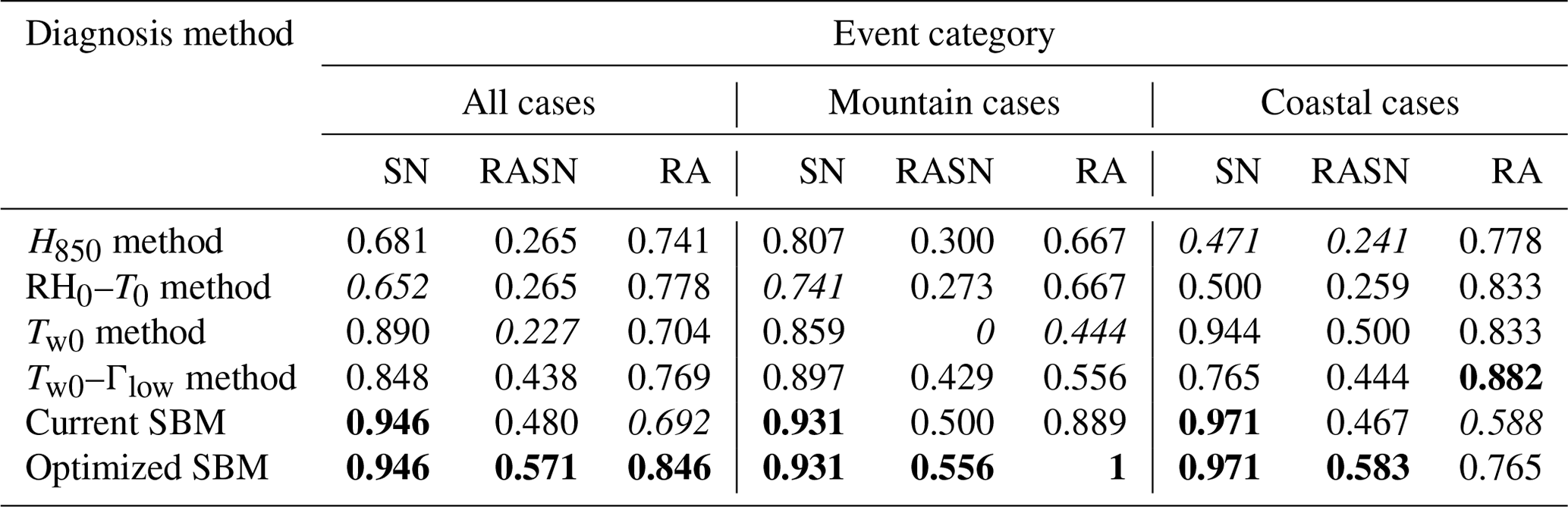
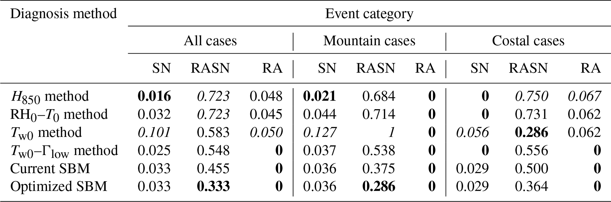
The CSI (Table 3) and FAR (Table 4) are calculated from Figs. 6, 7, and 8. The five diagnosis methods generally have lower CSI for RASN (0–0.583) and higher CSI for RA (0.667–1) and SN (0.471–0.971). Similarly, the FAR of the five diagnosis methods shows the highest false alarm rate for RASN (0.286–1) and the lowest false alarm rate for RA (0–0.067) and SN (0–0.127). The optimized SBM shows improved CSI as compared to the current SBM and the best performance for all WPT categories except RA at coastal sites. The FAR of the optimized SBM is only improved for RASN.

4.2 Dependence of diagnosis accuracy on wet-bulb temperature profiles

The environments of the coastal and mountain sites in the Pyeongchang region differ in many respects. In the coastal region, the low-level atmosphere is more humid and warmer than the mountain region due to the East Sea. The mountain region often has inversion layers near the surface due to radiative cooling, regional subsidence inversions, and cold-air damming. Near-surface inversion layers can strongly influence the accuracy of ground-based WPT diagnosis. The difference in the altitudes between the two regions also affects V_t because of differences in air density. Wind shear effects associated with specific synoptic wind patterns can enhance riming processes in the mountains of the Pyeongchang region (Kim et al., 2021). Therefore, we assess the impact of the atmospheric conditions on the performance of the five methods based on the characteristics of T_w profiles.

Figure 9 presents the observed WPTs based on the nomograms used for the four empirical methods. Figure 9a shows the distribution of observed WPTs using the H₈₅₀ method. The H₈₅₀ values for SN cases range from 1273 to 1305 gpm at the mountain sites and from 1269 to 1297 gpm at the coastal sites. The H₈₅₀ values for RA cases range from 1297 to 1329 gpm at the mountain sites and from 1289 to 1321 gpm at the coastal sites. The H₈₅₀ values for RASN cases range from 1294 to 1308 gpm at the mountain sites and from 1282 to 1302 gpm at the coastal sites. A large proportion of the H₈₅₀ values for RASN is distributed between H_SN and H_RA at both the mountain and the coastal sites. However, H₈₅₀ of many SN cases overlaps with that of RASN cases, with the overlap especially noticeable at the coastal sites.

Figure 9b presents RH₀–T₀ scatterplots with the shifted Matsuo scheme (Lee et al., 2014). Many SN cases are misdiagnosed as RASN due to the low T₀ threshold value when RH₀>85 %. Thus, we can speculate that the advection of low-level warm and humid air ($T_{\mathrm{0}}=\sim \mathrm{0}$ °C; RH₀>85 %) during snow is likely to increase its misdiagnosis as RASN.

Figure 9c displays the distribution of observed WPTs using T_w0. The dashed lines at T_w0=0.5 °C and T_w0=1.8 °C represent the thresholds suggested by Häggmark et al. (2000). T_w0 of SN cases ranges from −6 to 1 °C and that of RA cases ranges from −1 to 3.5 °C for the mountain sites compared to −6 to 0 °C and 1 to 5.5 °C for the coastal sites, respectively. T_w0 for RASN cases at the mountain sites ranges from −2 to 0.5 °C. A broad overlap of RASN and other WPTs highlights the difficulty in diagnosing WPTs in mountain regions with a single T_w0 threshold. In contrast, the distributions of WPTs as a function of T_w0 are much more clearly separated at the coastal sites.

Figure 9d presents the two-dimensional distribution of observed WPTs based on the T_w0–Γ_low method with a threshold snow probability of 0.1 and 0.9 (Sims and Liu, 2015). Γ_low of RA varies widely, though it tends toward positive values. However, three RA cases with T_w0>0 °C and ${\mathrm{\Gamma }}_{\mathrm{low}}<-\mathrm{2}$ °C km⁻¹ have a ground inversion layer at the mountain sites and two of them are misdiagnosed as RASN. In addition, two mountain cases are misdiagnosed as RA with high Γ_low (>8 °C km⁻¹). One is possibly FZRA ($T_{\mathrm{w}\mathrm{0}}\sim -\mathrm{1}$ °C), and the other (T_w0: ∼ 1 °C) indicates the presence of a complex atmospheric vertical structure (i.e., a melting layer aloft and near-surface refreezing layer). An RASN case with a T_w0 of around −2 °C and a Γ_low of ∼ 8.5 °C km⁻¹ also requires investigation into the atmospheric vertical structure.

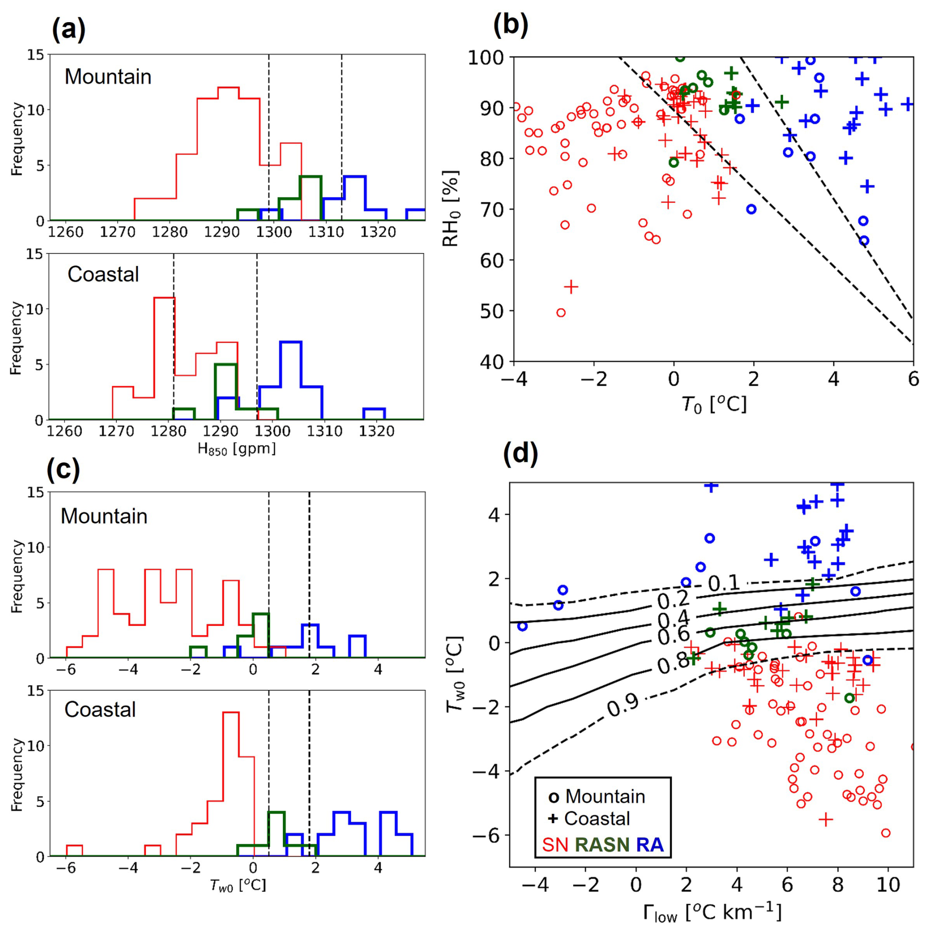
Figure 9 Representation of observed WPTs (colors) on (a) H₈₅₀ histogram, (b) RH₀–T₀ scatterplots, (c) T_w0 histogram, and (d) T_w0–Γ_low scatterplots. The colors indicate observed WPTs: SN (red), RASN (green), and RA (blue). The circles (crosses) indicate mountain (coastal) sites. The dashed lines indicate the threshold values for diagnosing WPTs.

The performance of each diagnosis method is also investigated as a function of the atmospheric vertical structure (i.e., the T_w profile) (Figs. 10–12). Figure 10a and b display the T_w profiles for observed SN cases at the mountain and coastal sites, respectively, with bold lines indicating misdiagnosed cases. Figure 10 shows that characteristics of the T_w profile below 1 km a.g.l. strongly influence the performance of all five diagnosis methods for SN cases. The H₈₅₀ and RH₀–T₀ methods tend to misdiagnose SN as RASN when relatively warm conditions are present below 1 km a.g.l. This tendency is especially noticeable at coastal sites, suggesting that SN cases with relatively warm and moist environments are frequently observed at coastal sites in the Pyeongchang region. These cases can be accurately diagnosed as SN by using T_w0 as the threshold instead of T₀. The T_w0–Γ_low method tends to misdiagnose the WPT in some warm environments with low vertical lapse rates that occur at coastal sites, indicating that a slight adjustment of the T_w0 threshold is required. The two SN cases misdiagnosed by the SBM at the mountain sites have a very thin (<50 m depth) near-surface warm layer (WL; a layer with T_w>0 °C in this study), highlighting a potential need for slightly increasing the wet-bulb temperature threshold used to partition SN from RASN for very shallow near-surface warm layers.

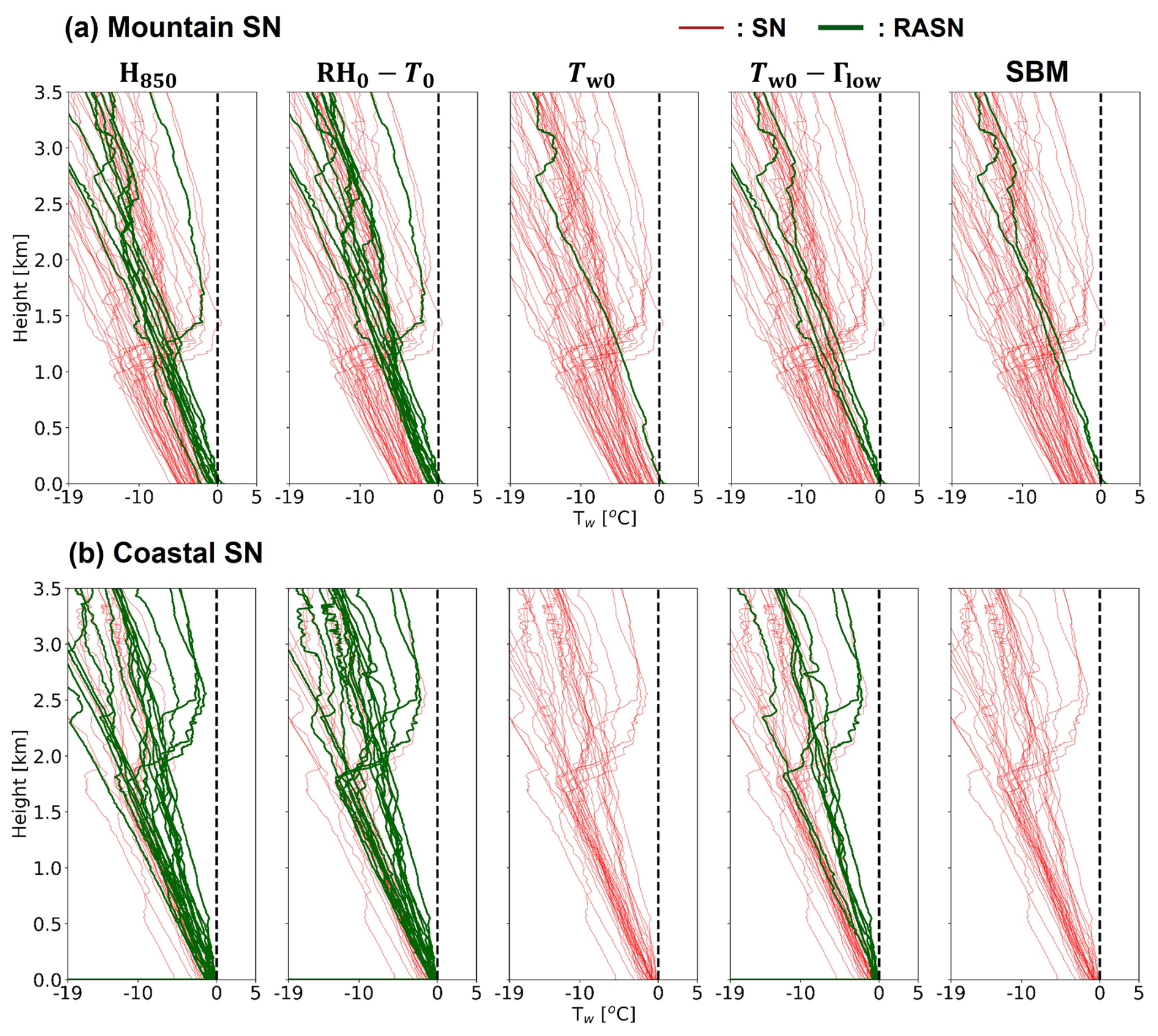
Figure 10 T_w profiles for observed SN cases occurring at (a) mountain sites and (b) coastal sites. The blue, red, and green lines indicate diagnosed RA, SN, and RASN cases, respectively, for the H₈₅₀ thickness, shifted Matsuo scheme using the RH₀–T₀ method, wet-bulb temperature T_w0, the T_w0–Γ_low method, and the current SBM methods. Bold lines indicate misdiagnosed cases.

Figure 11a and b present the T_w profiles of the mountain and coastal sites, respectively, for RASN cases. The ground temperature for mountain RASN cases tends to be colder than that for coastal RASN cases, which strongly influences the performance of the wet-bulb temperature method. An RASN case at the mountain site MOO (21:00 UTC on 4 March 2018; the same as the cold-RASN case with a T_w0 of approximately −2 °C and a Γ_low of ∼ 8.5 °C km⁻¹) is misdiagnosed by all five methods. The T_w profile of this case has an isothermal layer at 1.7–2.2 km a.g.l. with a T_w of about −0.5 °C. However, the PARSIVEL data clearly reveal the presence of liquid-phase particles (F_RA=42.55 %). We assume that melting occurs in the isothermal layer, although there are no data revealing the presence of a warm layer, such as vertically pointing radar data, at MOO. The SBM misdiagnoses two mountain RASN cases and a coastal RASN case as SN. These cases have a near-surface T_w very close to 0 °C but slightly less than 0 °C.

Figure 11 As in Fig. 10 but for observed RASN cases.

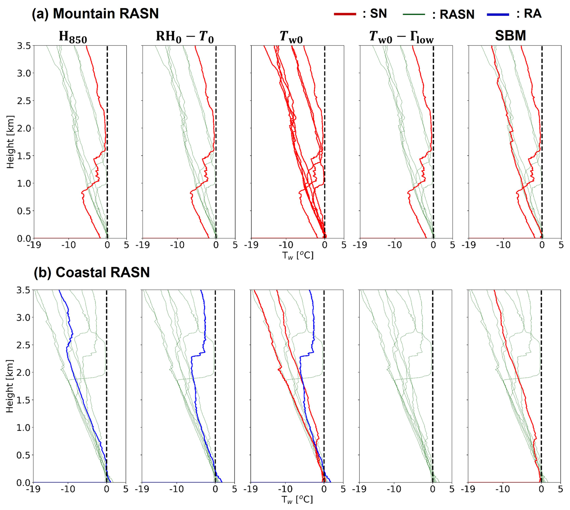
Figure 12a and b present the T_w profiles for the mountain and coastal sites, respectively, for RA cases. Many RA cases at the mountain sites have a deep warm layer and an inversion layer below 1.5 km a.g.l. (the dotted black oval in Fig. 12a), whereas RA cases with a shallow warm layer and no inversion layer frequently occur at the coastal sites (the dotted black oval in Fig. 12b). The SBM performs well in the former scenario but poorly in the latter. Other methods produce the opposite results, with superior performance at the coastal sites. The presence of inversion layers makes diagnosis based solely on ground conditions difficult. The SBM simulations sufficiently melt all particles within deep warm layers (i.e., 500–1500 m) in the former scenario. However, some cases of misdiagnosed RA have relatively shallow warm-layer depths (<500 m). The SBM simulations diagnose RASN for these cases because of the incomplete melting of large particles. For some cases with complex atmospheric profiles, the SBM diagnoses RASN for FZRA-like cases (the red arrow in Fig. 12a) with a single warm layer and single cold layer (a layer with T_w<0 °C below the warm layer in the present study) and for two cases with double warm layers and a single cold layer (the red arrow in Fig. 12b).

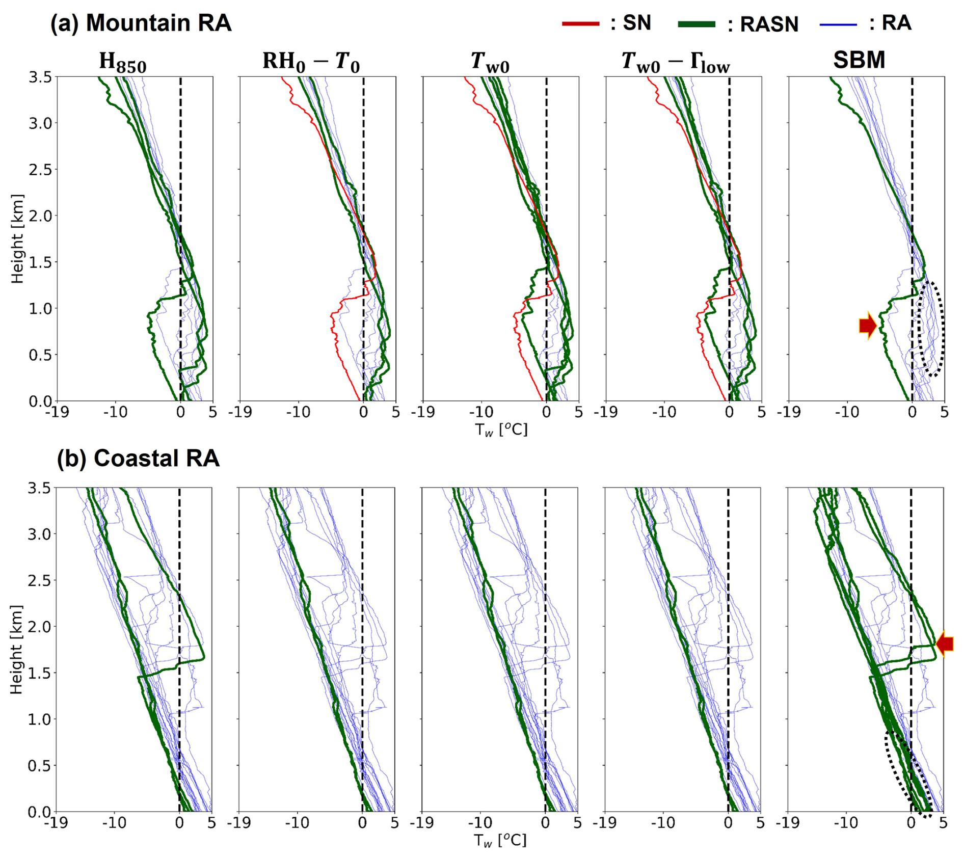
Figure 12 As in Fig. 10 but for observed RA cases. The arrows denote misclassified profiles that are discussed further in Sect. 4.2. The bold red line represents a case misdiagnosed as SN, while the thicker green line represents cases misdiagnosed as RASN.

4.3 Analysis of the misdiagnosed cases and optimization of the spectral bin model

Overall, the SBM misdiagnoses two observed SN cases, three observed RASN cases, and eight observed RA cases. The misdiagnosed SN cases have a very shallow warm layer near the ground. The misdiagnosed RASN cases have no warm layer in the T_w profile, but the maximum T_w in the sounding profile is very close to 0 °C. We hypothesize that observation or representativeness errors in the sounding may play an important role in the misdiagnosis of these SN and RASN cases. For example, there are hardware errors in the rawinsonde sensor. Changes in the rawinsonde path due to variation in wind speed and/or direction can also influence the diagnosis of the WPT because the atmosphere is not homogeneous.

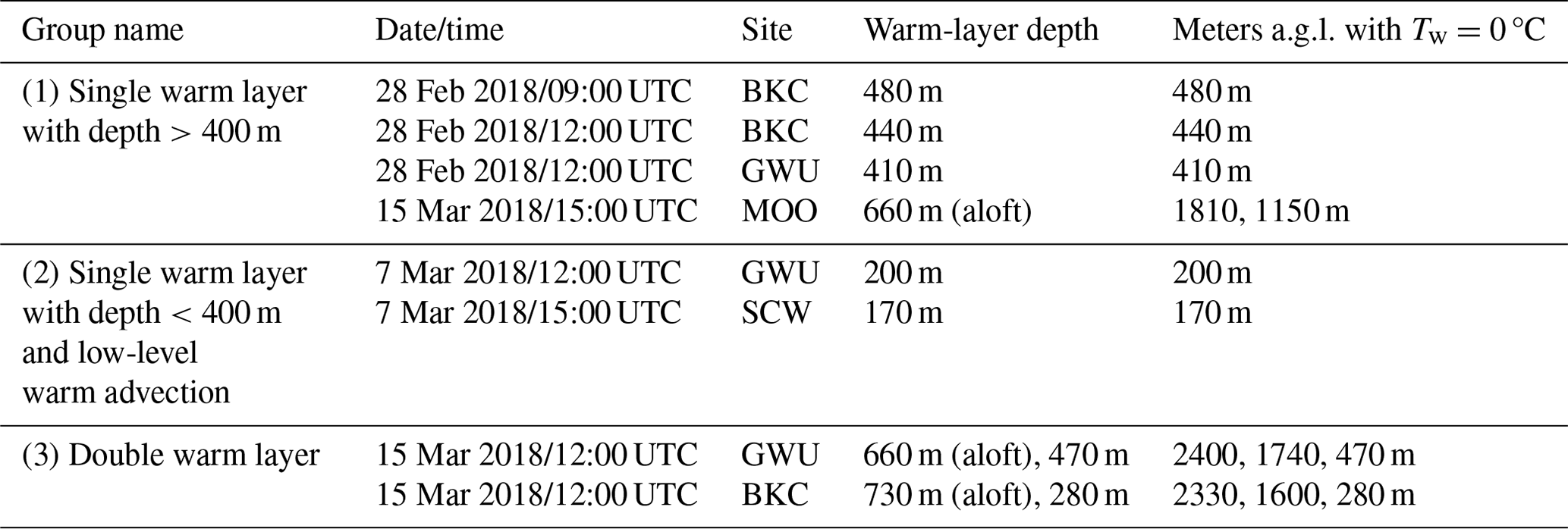
The eight misdiagnosed RA cases are listed in Table 5. Warm-layer depth is defined as the depth of the layer with T_w>0 °C in the T_w profile. We divide the cases into three groups according to the warm-layer depth and the number of warm layers: (1) a single warm layer with a depth of more than 400 m, (2) a single warm layer with a depth of less than 400 m and low-level warm advection, and (3) double warm layers. Group 1 has a warm layer with a depth of 400–600 m, Group 2 has a warm layer with a depth of 200–400 m and southerly flow at low levels, and Group 3 has a cold layer between a surface warm layer and a higher warm layer.

Table 5 The description of RA cases misdiagnosed by the SBM. Here, warm-layer depth is defined as the depth of the T_w>0 °C layer in the profile. “Aloft” indicates that the layer is not adjoined to the surface.

Only a representative example from each group is shown because each group has similar atmospheric environmental characteristics. We also compare the simulation results between the current and optimized SBMs. Figure 13 presents the environmental profiles from the rawinsondes and V_t–D scatterplots from the corresponding PARSIVEL taken at around 12:00 UTC on 28 February 2018 from GWU in Group 1 (Fig. 13a, d), 12:00 UTC on 7 March 2018 from GWU in Group 2 (Fig. 13b, e), and 12:00 UTC on 15 March 2018 from GWU in Group 3 (Fig. 13c, f). A wide distribution of raindrop sizes (D_max: ∼ 4.25 mm) following the RA curve is presented in Fig. 13d for a 400 m warm layer with strong easterly winds (Fig. 13a). In contrast, a narrow raindrop size distribution (D_max: ∼ 1.62 mm) following the RA curve is displayed in Fig. 13e for a 200 m warm layer with strong low-level southerly winds (Fig. 13b). Figure 13f also shows a relatively narrow raindrop size distribution (D_max: ∼ 2.5 mm) with the matched profile characterized by an elevated warm layer and another warm layer near the ground (Fig. 13c).

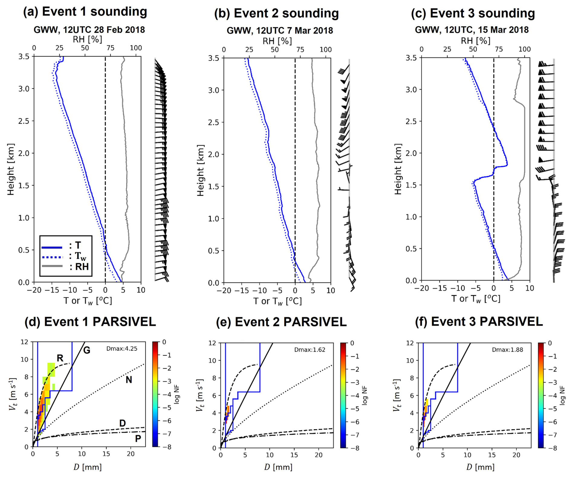
Figure 13 Environmental profiles (a–c) from rawinsondes and (d–f) V_t–D scatterplots from PARSIVELs for Event 1, Event 2, and Event 3, respectively. The solid (dotted) blue line in the environmental profile indicates T (T_w), and the solid gray line is RH. “P” (plate), “D” (dendrite), “G” (graupel), and “N” (needle) in the scatterplots depict empirical size–fall speed relationships suggested by Lee et al. (2015). “R” (raindrop) is the empirical relationship suggested by Atlas et al. (1973). The Yuter et al. (2006) scheme is marked with a solid blue line in the scatterplots.

Figure 14 presents the relationship between the height and liquid water fraction (f_w) for the current and optimized SBMs as a function of the particle size for the cases shown in Fig. 13. The simulation results from the current SBM for Event 1 show the incomplete melting of large particles (>1.75 mm) (Fig. 14a), whereas the f_w distribution from the optimized SBM shows complete melting of all particles at 200 m a.g.l. (Fig. 14e). The simulation results for Event 2 show that particles with a D_w of ≤1.05 mm completely melt in the current SBM compared with 1.35 mm for the optimized version (Fig. 14b and f); the optimized SBM simulation significantly increases the amount of melting. However, the maximum diameter with complete melting (∼ 1.35 mm) in the simulation is still slightly smaller than the observed D_max (∼1.62 mm). This difference could be the result of three sources of error: northward advection of the rawinsonde due to low-level southerly winds, hardware calibration issues for the GWU PARSIVEL, and/or the growth of raindrops via a collision–coalescence process. Collision–coalescence is also an important factor for the classification of WPT because the process increases the average raindrop size and decreases the number concentration of small drops. However, this process is not currently included in the SBM owing to algorithm efficiency demands, but it is a major area for future improvement.

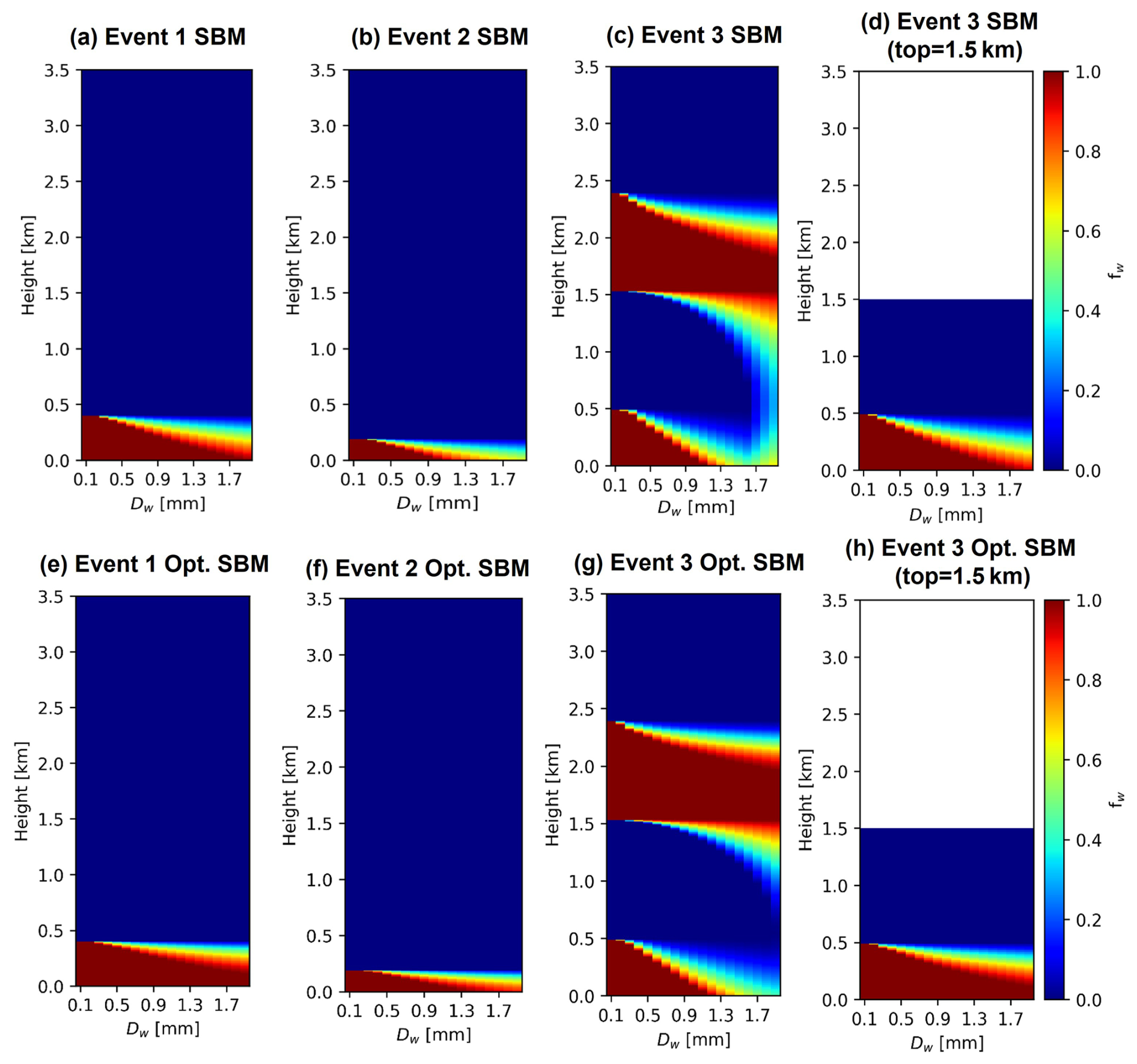
Figure 14 Liquid water fraction distribution as a function of height and D_w for Event 1, Event 2, and Event 3. (a–d) Simulation results of the SBM. (e–g) Simulation results of the optimized SBM.

Simulation results for Event 3 (Fig. 14c and g) show melting, refreezing, and additional melting during the descent of the particles from the cloud top to the ground. At the surface, the melting of large particles is incomplete in both the current SBM and the optimized SBM, although a deep warm layer (depth: ∼ 500 m) below the cold layer is present. The SBM assumes that the fall speed of the particles undergoing refreezing follows the relationship for IPs suggested by Kumjian et al. (2012). Because IPs generally have a larger density and fall velocity than snowflakes, the melting speed for IPs is relatively slow. To better understand Event 3, we analyzed MRR data. Figure 15 presents the time–height series for Z and −V_r observed by the MRR at GWW on 15 March 2018. Near the sounding time, the precipitation system drastically changes from a shallow system (cloud top of ∼ 1.5 km a.g.l.) to a seeder–feeder system (cloud top of ∼ 3.5 km a.g.l.) (Fig. 15a and b). It is possible that the rawinsonde sensor passed the feeder–seeder system, but the ground precipitation observed by the PARSIVEL appears to originate from the shallow system observed earlier in the time series. Indeed, the Doppler fall velocities measured by the MRR from the sounding time onward between 1.0 and 1.5 km a.g.l. are relatively slow and are unlikely to correspond to IPs as suggested by the SBM when initialized with a higher cloud top (Fig. 14c, g). Therefore, we re-run the SBM simulation with the cloud top set to 1.5 km. The simulation results from this new run are shown in Fig. 14d and h. Both the SBM and the optimized SBM show an increase in melting amount in the warm layer near the ground compared to those in Fig. 14c and g, with the optimized SBM simulating the complete melting of all particles by 200 m a.g.l.

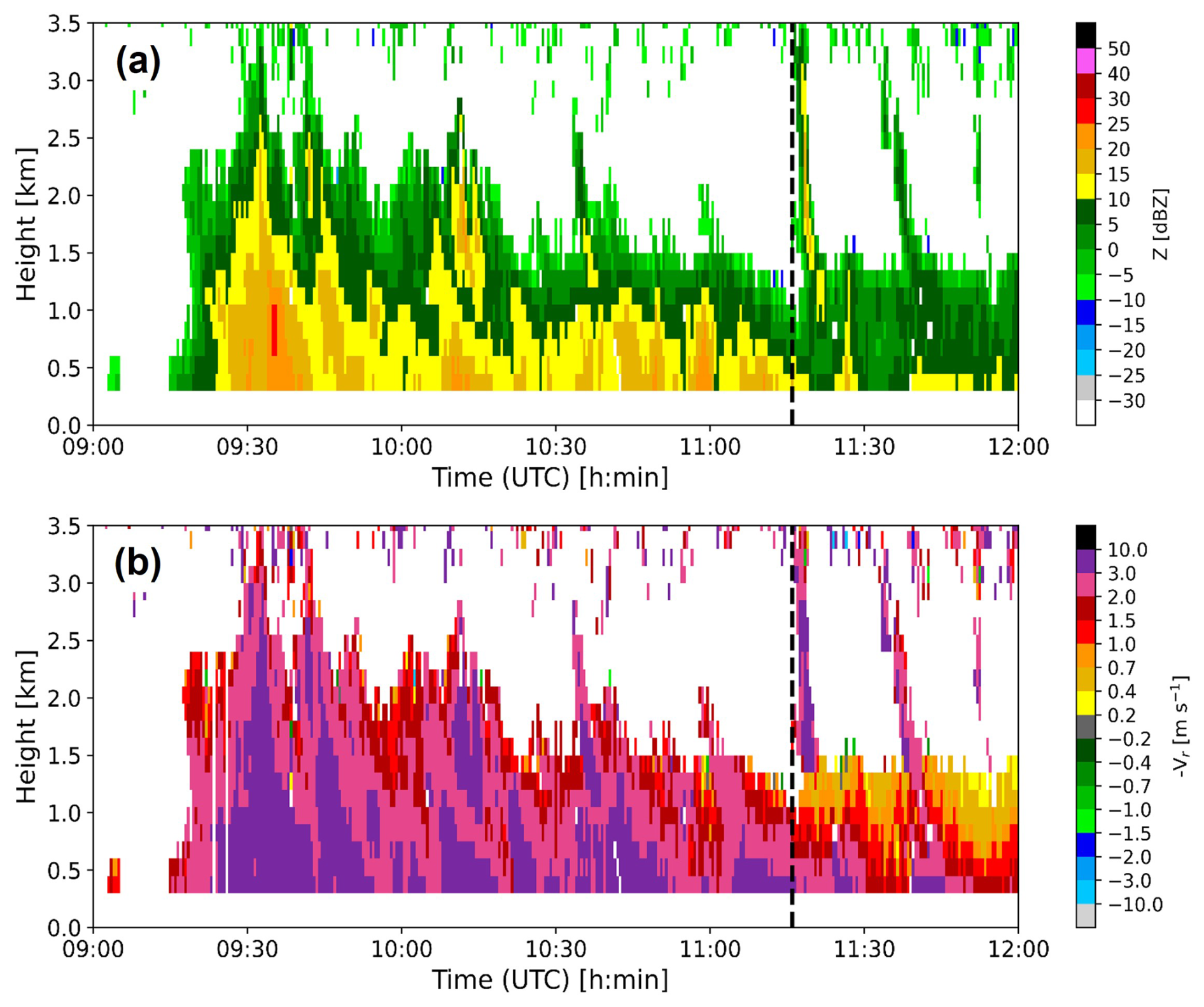
Figure 15 (a) Z and (b) −V_r time series observed from the MRR in GWW on 15 March 2018. The dotted line indicates the sounding start time of Event 3.

In summary, the potential main causes of the misdiagnosis of RA cases when using the SBM are suboptimal microphysical assumptions and sources of error in the input data. Optimization of the microphysics scheme using data from the Pyeongchang region significantly increases the amount of melting compared to simulations using the current microphysics scheme in the SBM. Among the eight misdiagnosed cases in the SBM, four are correctly diagnosed by the optimized SBM. If a more accurate cloud top is also considered, two more cases are correctly diagnosed by the optimized SBM. These results indicate that using accurate cloud top information can produce more reasonable SBM simulations. Although Group 2 cases are still misdiagnosed by the optimized SBM, the simulation accuracy could be further improved if information on horizontal advection and the maximum particle size is considered.

5 Summary and future work

The performance of the SBM in diagnosing WPTs was evaluated through a comparison with other empirical/statistical methods (H₈₅₀ method, RH₀–T₀ method, T_w0 method, and T_w0–Γ_low method) for 131 matched precipitation cases during the ICE-POP 2018 period. The observed WPTs were determined from 5 min PARSIVEL data using a newly designed decision tree algorithm. This algorithm classified the three WPTs – SN, RASN, and RA – using F_RA and F_SN based on the Yuter et al. (2006) scheme and manual analysis of V_t–D scatterplots. The WPTs diagnosed by the five methods were obtained using matched sounding data. A simplified WPT classification scheme for the SBM using R and SR was used, even though the SBM can classify additional WPTs. Various skill scores (h, h^′, h_SN, h_RASN, h_RA, CSI, and FAR) were calculated to evaluate the performance of the diagnosis methods. In addition to the overall skill scores, the effect of the WPTs (SN, RASN, and RA), terrain (i.e., mountain vs. coastal sites), and atmospheric vertical structure (T_w profiles) on the performance of the compared methods was examined.

The current SBM (which ranked first for h) and the T_w0–Γ_low method approach (which ranked first for h^′) achieved higher scores than the other methods for all matched precipitation cases. The accuracy of the SBM was the highest for the mountain sites, whereas the accuracy of the T_w0 and T_w0–Γ_low methods was the highest for the coastal sites. Coastal SN cases featuring relatively warm and moist environments can lead to misdiagnosis when using the H₈₅₀ and RH₀–T₀ methods. Most of the RASN cases that occurred at the mountain sites were characterized by a very shallow warm layer near the surface. These cases led to poor diagnosis using the wet-bulb temperature method. Ground-based or low-level-based methods showed low accuracy for mountain RA cases with a near-ground inversion layer, whereas the SBM performed well for these cases. Conversely, the SBM exhibited relatively poor accuracy for some coastal RA cases with a warm-layer depth of less than 500 m. These results suggest that SBM simulations tend to produce less melting compared to the observed precipitation.

The microphysics scheme used in the SBM was evaluated by analyzing three groups of misdiagnosed RA cases: those with a single warm layer with a depth more than 400 m, those with a single warm layer with a depth less than 400 m and low-level warm advection, and those with double warm layers. We also attempted to optimize the microphysics scheme of the SBM using a region-specific density–diameter relationship and compare the simulations between the current and optimized SBMs for the three groups. Overall, the optimized SBM demonstrated an increased amount of melting and improved skill scores (h, h^′, CSI for RASN and RA, FAR for RASN) compared to the current SBM. The optimized SBM also correctly diagnosed the WPT of the double warm-layer group when more representative cloud top height data were used.

The potential of the SBM for diagnosing the WPT was thus confirmed in the present study. The performance of the current SBM was superior to some existing optimized methods (the H₈₅₀ and RH₀–T₀ methods), and the skill scores were improved further via regional optimization of the SBM's microphysics scheme. Furthermore, there is a need to verify the microphysics scheme in the SBM in more detail, such as for IP events. We will focus on the development of a combined SBM with three-dimensional reanalysis field data (e.g., Local Data Assimilation and Prediction System) for the acquisition of three-dimensional WPT information. Accurate three-dimensional WPT information will be helpful for various fields, such as aviation warning and understanding the detailed structure of the cloud/precipitation system.

Appendix A: List of abbreviations

1DSBM	One-dimensional spectral bin model
a.g.l.	Above ground level
a.m.s.l.	Above mean sea level
AWS	Automatic weather station
BKC	Bokwang1-ri Community Center
CFAD	Contoured frequency by altitude diagram
CSI	Critical success index
DGW	Daegwallyeong Regional Weather Office
FAR	False alarm rate
FMCW	Frequency modulated continuous wave
FZRA	Freezing rain
GPM	Global precipitation measurement
GWU	Gangneung-Wonju National University
GWW	Gangwon Weather Administration
HRRR	High-Resolution Rapid Refresh
ICE-POP	International Collaborative Experiments for Pyeongchang 2018 Olympic and Paralympic winter games
IP	Ice pellet
IPFZRA	Mixture of ice pellets and freezing rain
MOO	Myeonon Observatory
MRR	Micro rain radar
NF	Normalized frequency
PARSIVEL	Particle size velocity
PDF	Probability density function
PSD	Particle size distribution
RA	Rain
RASN	Mixture of rain and snow
RH	Relative humidity
SBM	Spectral bin model
SCW	Sokcho Weather Administration
SN	Snow
T	Temperature
WPT	Winter precipitation type
WTLS	Weighted total least square