Using automatic calibration to improve the physics behind complex numerical models: an example from a 3D lake model using Delft3D (v6.02.10) and DYNO-PODS (v1.0)

Models are simplified descriptions of reality and are intrinsically limited by the assumptions that have been introduced in their formulation. With the development of automatic calibration toolboxes, finding optimal parameters that suit the environmental system has become more convenient. Here, we explore how optimization toolboxes can be applied innovatively to uncover flaws in the physical formulations of models. We illustrate this approach by evaluating the effect of simplifications embedded in the formulation of a widely used hydro-thermodynamic model. We calibrate a Delft3D model based on temperature profiles for a case study, Lake Morat (Switzerland), through the DYNO-PODS optimization tool. The results show that higher values of the light extinction coefficient can compensate for neglecting the fraction β of short-wave radiation absorbed at the surface of the water. This leads to unrealistic values of the light extinction coefficient, as the optimization pushes its value toward the limit of no transparency, consistent with the need to reproduce a significant absorption at the surface. Although it is well known that β is significantly larger than zero, its absence from the model was never noticed as critical. Automatic calibration tools provide valuable diagnostic insights into the physical robustness of models, enabling more precise evaluation of their structural integrity and performance.

1 Introduction

Numerical models serve as powerful tools capable of embracing the complexity of intricate environmental dynamics. In many branches of environmental science, such as meteorology, climatology, hydrology, oceanography, and limnology, hydro-thermodynamic models have become standard tools to simulate and understand specific physical processes. These models are rooted on the numerical solution of physical first principles, e.g., the mass, momentum, and heat equations. Although first principles are well established, modeling the physics of fluid systems remains complicated for two reasons. First, the grid size limits the range of applicability of models based on first principles (e.g., direct numerical simulation, DNS) and poses the challenge to properly parameterize associated sub-grid-scale processes. This implies that models that were developed for a specific environment, where the parametrization was adequate, may not be optimized for other contexts characterized by different spatial scales. Second, imposing the boundary conditions is a complicated task as the forcing acting at the boundaries of the computational domain is often only partially known. For instance, the estimation of the surface heat fluxes is based on parametrizations that have to cope with both the complex physics and the uncertainties associated with the forcing. Contrary to the first principles solved by the model, such boundary conditions often lack universality. In the specific case of models widely adopted to simulate three-dimensional lake dynamics, many were originally developed for marine, riverine, or estuarine environments. This is the case, for example, with Delft3D (Lesser et al., 2004), MITgcm (Marshall et al., 1997), ROMS (Shchepetkin and McWilliams, 2005), FVCOM (Chen et al., 2003), NEMO (Madec et al., 2023), and POM (Blumberg and Mellor, 1987), among a few others. Therefore, some processes that are crucial in lakes but not for the original environment may be correctly reproduced. Scientists thus must critically evaluate model performances, as even some of the most used models may have unexpected flaws.

The first step of any model setup and performance evaluation is calibration. Tools for the automatic calibration of the model parameters have recently been introduced, enabling a broader and more efficient search for the optimal parameters. Analyses of how these tools can provide support and foster a better understanding of the numerical results are becoming increasingly frequent. For instance, examples are numerous for the Delft3D model (in particular, the FLOW module), one of the most popular models for simulating hydrodynamics of natural environments. Garcia et al. (2015) and Baracchini et al. (2020b) adopted a derivative-free algorithm for non-linear least squares (DUD from Ralston and Jennrich, 1978) within OpenDA (El Serafy et al., 2007) to optimize calibration and data assimilation in their lake models, Schwindt et al. (2022) assessed the uncertainty of mixing-related model parameters through a Bayesian calibrator combined with a Gaussian process emulator, and Xia et al. (2021, 2022) developed the PODS tool (Parallel Optimization with Dynamic coordinate search using Surrogates) and showed the potential of using surrogate models to accelerate global optimization. A surrogate model, also known as emulator, is a simplified and computationally efficient empirical model (Castelletti et al., 2010) that mimics the behavior of a computationally expensive model based on real model training data. In the search for the optimal parameters, the largest computation cost is indeed related to the real model runs. Thus, fast surrogate model runs are alternated with real model runs such that a lower number of real model evaluations is needed. Surrogate models can be included in traditional optimization tools such as Bayesian calibration (Ma et al., 2024) and are highly effective in speeding up the calibration process.

Many opportunities are offered by automated calibrators, saving time and finding global optimal solutions, and many other optimization algorithms have been applied for the calibration of hydrodynamic models. We refer to Xia et al. (2021) for a review of all these aspects. However, much care must be taken when model parameters are calibrated, either manually or automatically. The literature reports examples where calibration has guided modelers in regions of the parameter space that hold no physical meaning (e.g., Baar et al., 2019, well discussed by Tritthart et al., 2024). Such unrealistic parameters are often justified as those giving the best model performance, but it is well known that (i) a different combination of parameters might give the same result, and (ii) the performance of the model heavily depends on what metric is adopted. This is particularly true for hydro-thermodynamic models calibrated on a single variable, e.g., temperature profiles only (Amadori et al., 2021; Xia et al., 2022). The objective of this work is to show how the use of automatic calibration can help identify flaws in the structure of even state-of-the-art models. Analyses of how these tools can foster a better understanding of the numerical results have started to appear in the literature. In the work previously cited by Schwindt et al. (2022), the authors were able to identify unrealistic model setups from the high uncertainty of the a posteriori distribution of mixing-related parameters. With a similar philosophy, here we evaluate the parametrization of the heat distribution along the water column as coded in Delft3D. In particular, we focus on the depth of the Secchi disk (Secchi, 1864, hereafter denoted as D_s or simply “Secchi depth”), as a parameter representing the transparency of the water. Considering water transparency in hydro-thermodynamic models has long been recognized as fundamental to enhance the prediction of water temperature (e.g., Henderson-Sellers, 1986; Zolfaghari et al., 2017; Shatwell et al., 2019), as it allows for the inclusion of biologically driven mechanisms, even when they are not explicitly parameterized. D_s is used to model the distribution of the incoming solar short-wave radiation from the surface to deeper layers, depending on how deep radiation can penetrate the water column. Although D_s is often considered a calibration parameter in models (e.g., Wahl and Peeters, 2014; Soulignac et al., 2017; Piccioni et al., 2021; Xia et al., 2021), it is actually a measurable quantity that can vary significantly over time and, in some cases, space . In large lakes, differences between onshore and offshore D_s measurements can be of the same order of magnitude as seasonal variations (e.g., Pothoven and Vanderploeg, 2020, found up to 4 times lower transparency in coastal waters compared to pelagic areas of Lake Michigan). Massive algal blooms, combined with basin-scale circulation, can also drive complex spatial patterns of water transparency as those observed by Rahaghi et al. (2024) in Lake Geneva, with D_s ranging between < 2 and > 6 m on the same day.

However, experience from previous Delft3D applications in various lakes shows that the calibrated value of D_s generally resides in the lower range of measured values (Wahl and Peeters, 2014; Soulignac et al., 2018), or it is even lower than the observed values (for example, Amadori et al., 2020 and Piccolroaz et al. (2019) rescaled the observed Secchi depth by a factor of 0.5). Through the DYNO-PODS automatic calibrator (Xia et al., 2022), we extend the search for the optimal D_s in a broader parameter space and explore uncharted regions for manual calibration. We demonstrate how this sheds light on a flaw in the heat flux parametrization of Delft3D and lets us improve the physics behind such a widely used model with a small, yet significant, modification to its source code.

In the following sections, we first formulate the problem (Sect. 2). There we summarize how Secchi depth is used in Delft3D (Sect. 2.1), how surface warming is generally simulated in models (Sect. 2.2), and what the physical implications of the current Delft3D parametrization (Sect. 2.3) and of the modified version we implemented are (Sect. 2.4). In Sect. 3, we introduce the calibration strategy and numerical experiments. In Sect. 4, we first show the results of the original formulation of the Delft3D heat flux scheme (Sect. 4.1). We then present the results of the calibration tests that point out the model's unexpected behavior (Sect. 4.2). Finally, we show the gain in physical reliability achieved after our modification of the Delft3D source code (Sect. 4.3).

2 Formulation of the problem

2.1 Use of Secchi depth in models

The three-dimensional model Delft3D-FLOW (Lesser et al., 2004) numerically solves the Reynolds-averaged Navier–Stokes (RANS) equations under the Boussinesq and shallow-water assumptions. The horizontal velocity components and the water surface are solved by integrating the continuity and horizontal momentum equations, while the vertical velocities are computed from the continuity equation. The transport of heat is modeled by an advection–diffusion equation, assuming that there is no heat exchange at the lake bed.

In the heat equation module of the model, all the heat flux terms are estimated with empirical formulas. Here, we focus on the penetration of solar short-wave radiation, which is modeled with a reduction of the energy flux per unit area (W m⁻²) along the water column, as in the commonly used Beer law:

$$\begin{array}{}\text{(1)}& H_{\mathrm{sw}}\left(z\right)=H_{\mathrm{sw}\mathrm{0}}\exp \left(-\mathit{\gamma }z\right),\end{array}$$

where H_sw0 is the downward short-wave radiation at the water surface (already considering the effect of albedo), H_sw(z) is the energy flux that reaches the depth z, and γ is the extinction coefficient (m⁻¹). This simplified model refers to the light attenuation coefficient, which can be easily measured in situ, and is appropriate for the region of the visible spectrum (380–750 nm). Accordingly, the extinction coefficient γ is defined based on the depth D_s (m) at which the Secchi disk remains visible, through the following simple relation:

$$\begin{array}{}\text{(2)}& \mathit{\gamma }={\displaystyle \frac{c_{\mathit{\gamma }}}{D_{\mathrm{s}}}},\end{array}$$

where the value c_γ=1.7 is used as standard in Delft3D (Deltares, 2023) and was originally proposed by Poole and Atkins (1929).

However, the actual penetration of the short-wave radiation depends on the different wavelengths that make up its spectrum. In principle, each wavelength has a different extinction coefficient (Zaneveld and Spinrad, 1980). Much of the short-wave radiation energy, in particular longer wavelengths in the near-infrared to the short-wave-infrared region (750–2500 nm), is absorbed at the water surface regardless of its optical properties. The water optical properties are indeed related to the concentration of constituents and mainly affect the extinction coefficient in the visible region (400–700 nm).

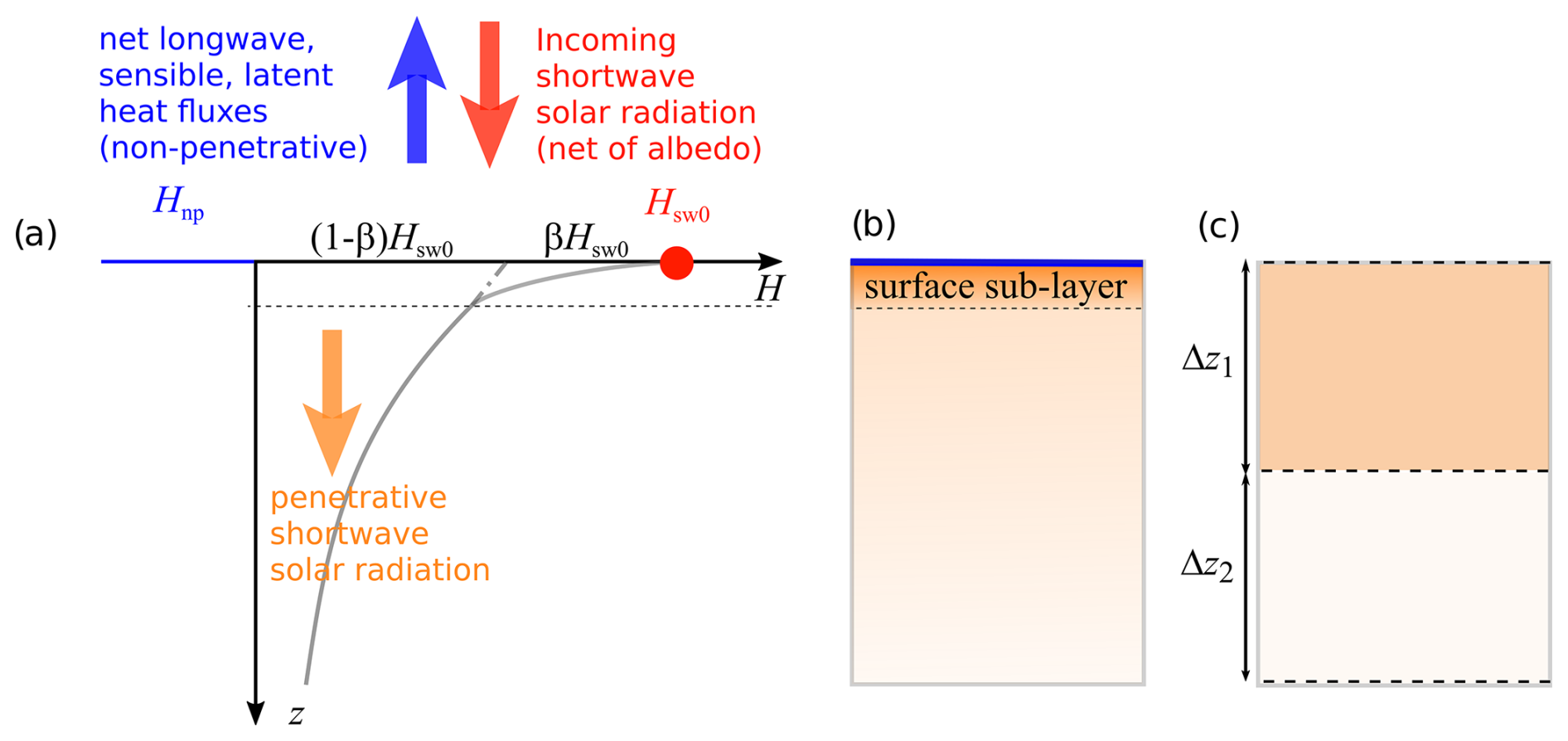
Figure 1 (a) Heat transfer at water surface. Non-penetrative terms H_np are lost at the air–water interface (blue line, representative of the skin layer), while a sub-layer at the surface retains a fraction β of incoming solar radiation H_sw0, and only the fraction (1−β)H_sw0 of the solar short-wave radiation penetrates along the water column. The two grey lines represent the exponential decay of incoming heat flux in the surface sub-layer (above the horizontal dashed line) and beneath it. (b) Conceptual illustration of how the process in (a) evolves along the water column, with orange representing heat penetrating from the surface to the deeper layers; (c) schematic of how (a) is then parameterized in a vertically layered computational grid.

Among many formulations available to properly describe the penetration of downward solar radiation in the water column (Morel and Antoine, 1994), the simplified version reported in Henderson-Sellers (1986) is commonly applied in many numerical models:

$$\begin{array}{}\text{(3)}& H_{\mathrm{sw}}\left(z\right)=\left(\mathrm{1}-\mathit{\beta }\right)H_{\mathrm{sw}\mathrm{0}}\exp \left(-\mathit{\gamma }z\right).\end{array}$$

In such a formulation, β is the fraction of the short-wave radiation absorbed in a region close to the surface.

As a consequence, the surface layer is warmed up by a localized total heat flux,

$$\begin{array}{}\text{(4)}& H_{\mathrm{surf}}=H_{\mathrm{np}}+\mathit{\beta }{H}_{\mathrm{sw}\mathrm{0}},\end{array}$$

which is the sum of the absorbed short-wave radiation β H_sw0 and of the other non-penetrative fluxes H_np (see Fig. 1). The non-penetrative heat flux,

$$\begin{array}{}\text{(5)}& H_{\mathrm{np}}=H_{\mathrm{lw}}^{\downarrow }-H_{\mathrm{lw}}^{\uparrow }\pm H_{\mathrm{sens}}\pm H_{\mathrm{lat}},\end{array}$$

is the result of the net downward long-wave radiative flux $H_{\mathrm{lw}}^{\downarrow }$ (from the sky to the lake), the upward long-wave radiation $H_{\mathrm{lw}}^{\uparrow }$ (emitted by the lake surface), and the sensible and latent heat fluxes (H_sens and H_lat), respectively. All these terms are associated with a generic surface heat flux H_surf, but it is worth noting that non-penetrative terms act just at the interface between water and air, while β H_sw0 is absorbed in a layer of the order of tens of centimeters (Henderson-Sellers, 1986) (Fig. 1b). From the viewpoint of numerical modeling (Fig. 1c), the fraction β of the incoming solar radiation represents a source of heat in a shallow layer of water, while non-penetrative terms (usually negative) represent a sink of heat, as will be shown later. All these fluxes are normally parameterized in only one computational cell, i.e., the one immediately below the water surface, where the contributions of both Eqs. (3) and (4) should be accounted for.

Modified versions of the Beer law were introduced in some lake-dedicated models to account for the different absorption rates of heat depending on the spectral bands of solar radiation. This is the case of the General Lake Model (Hipsey et al., 2019), where the authors attribute 55 % of the incident solar radiation to near-infrared (NIR) and ultraviolet (UVA, UVB) radiation heating the surface directly. A default value of 45 % for β is implemented in CE-QUAL-W2 (Cole and Wells, 2015), but different values of 24 % to 69 % are recommended depending on the type of environment, with higher values attributed to pure waters (63 %) and coastal waters (69 %) and lower values (24 % to 58 %) to lake waters. A similar approach with different proportions (35 % for NIR, 65 % for PAR¹ , UVA, UVB) was adopted by Thiery et al. (2014) to simulate the thermal structure of Lake Kivu with an ensemble of different lake models. Among these, models explicitly including β are SimStrat (Goudsmit et al., 2002), LAKEoneD (Joehnk and Umlauf, 2001), LAKE (Stepanenko and Lykossov, 2005), and MINLAKE96 (Fang and Stefan, 1996).

Although accounting for this fraction of heat at the surface is important in lakes, to the best of our knowledge the absence of this term in Delft3D never raised any concern in its previous applications to lacustrine environments. The reason is that the extinction coefficient γ estimated with Eq. (2) (or equivalently the depth of the Secchi disk D_s) is considered a calibration parameter, even if D_s is a measurable quantity.

2.2 General formulation of surface layer warming

Hydro-thermodynamic models such as Delft3D solve a thermal energy balance, where the heat source is usually dominated by the heat exchanged at the air–water interface. The relevant terms in the equation for the transport of heat can be represented as follows:

$$\begin{array}{}\text{(6)}& {\displaystyle \frac{\partial T}{\partial t}}+\mathrm{advection}+\mathrm{diffusion}=-{\displaystyle \frac{\partial \mathit{\varphi }}{\partial z}},\end{array}$$

where T is water temperature and ϕ is the vertical heat flux. We assume that the vertical coordinate z is pointing downward, such that the heat flux is positive downward (consistent with the direction of solar radiation). The source term on the right-hand side of the equation represents the local heating, which depends on the absorption of the radiative heat flux. Without this source term, the advection and diffusion terms can only redistribute the heat in the domain, so the total heat content of the lake is conserved if no flux is exchanged at the boundaries.

In Eq. (6), we have simplified the notation by introducing the flux (units K s⁻¹m)

$$\begin{array}{}\text{(7)}& \mathit{\varphi }={\displaystyle \frac{H}{\mathit{\rho }{c}_{\mathrm{p}}}},\end{array}$$

which scales the total heat flux H with water density ρ (units kg m⁻³) and specific heat capacity at constant pressure c_p (units $\mathrm{J}{\mathrm{kg}}^{-\mathrm{1}}{\mathrm{K}}^{-\mathrm{1}}$), assuming them to be constant, as a first approximation. Hereafter, the definition of ϕ_x based on Eq. (7) is adopted for all heat fluxes H_x, where the subscript x indicates the component.

The net heat flux at the air–water interface is

$$\begin{array}{}\text{(8)}& {\mathit{\varphi }}_{\mathrm{net}}={\displaystyle \frac{H_{\mathrm{net}}}{\mathit{\rho }{c}_{\mathrm{p}}}}={\mathit{\varphi }}_{\mathrm{sw}\mathrm{0}}+{\mathit{\varphi }}_{\mathrm{np}}=(\mathrm{1}-\mathit{\beta }){\mathit{\varphi }}_{\mathrm{sw}\mathrm{0}}+{\mathit{\varphi }}_{\mathrm{surf}}.\end{array}$$

In a depth-averaged model, the net heat flux is responsible for the change of the whole-lake temperature. Neglecting the sub-daily variability, the warming of the lake is related to the total heat exchanged during a day:

$$\begin{array}{}\text{(9)}& \underset{\mathrm{diel}}{\int }{\mathit{\varphi }}_{\mathrm{net}}\mathrm{d}t=\underset{\mathrm{diel}}{\int }{\mathit{\varphi }}_{\mathrm{np}}\mathrm{d}t+\underset{\mathrm{sunlight}}{\int }{\mathit{\varphi }}_{\mathrm{sw}\mathrm{0}}\mathrm{d}t,\end{array}$$

where the integrals are defined on a 24 h period (covering the periods of sunlight, with ϕ_sw0>0, and night, with ϕ_sw0=0). The total exchanged heat, ∫_dielϕ_net dt, is typically much smaller than the two individual components on the right-hand side of Eq. (9), as can be seen in Fig. 2a. Under these conditions (and to illustrate the behavior of the system), it can be assumed that ${\int }_{\mathrm{diel}}{\mathit{\varphi }}_{\mathrm{net}}\mathrm{d}t\simeq \mathrm{0}$. Therefore, the non-penetrative heat lost through the surface must approximately balance the solar heating (i.e., ${\int }_{\mathrm{diel}}{\mathit{\varphi }}_{\mathrm{np}}\mathrm{d}t\simeq -{\int }_{\mathrm{sunlight}}{\mathit{\varphi }}_{\mathrm{sw}\mathrm{0}}\mathrm{d}t$) so that the non-penetrative components of the heat flux have a cooling effect in most cases. In terms of diel averaged values (indicated using angle brackets), the condition can be written as

$$\begin{array}{}\text{(10)}& \langle {\mathit{\varphi }}_{\mathrm{np}}\rangle \simeq -{\displaystyle \frac{\mathrm{1}}{{\mathit{\tau }}_{\mathrm{day}}}}\underset{\mathrm{sunlight}}{\int }{\mathit{\varphi }}_{\mathrm{sw}\mathrm{0}}\mathrm{d}t<\mathrm{0},\end{array}$$

where τ_day is 24 h. Since the sub-daily variability of the non-penetrative fluxes is small compared to the solar radiation flux, it follows that ϕ_np≃〈ϕ_np〉 (see, for example, the example in Fig. 2), and Eq. (8) implies that lakes are typically subject to (relative) cooling during night and to (relative) warming during sunlight.

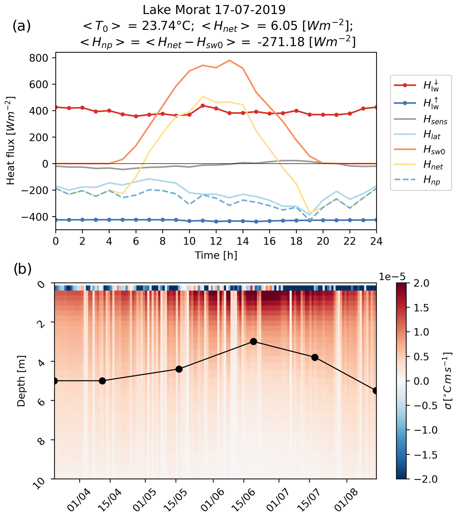
Figure 2 (a) Heat fluxes computed using the meteorological forcing and the simulated surface water temperature from the base setup model (𝒪 in Table 1) for Lake Morat on a sample summer day, i.e., 17 July 2019. (b) Warming rates simulated along the water column were calculated according to Eqs. (14)–(15) using the flux calculated by model 𝒪. Profiles are displayed at 12:00 UTC. The black line represents the measured Secchi depth (D_s) considered in the simulation, with black dots indicating the exact measurement day. Depths are limited to 10 m to improve visibility of the surface layer.

The numerical model solves the discretized form of the heat equation (Eq. 6) in an ith layer of thickness Δz_i. If the advective and diffusive fluxes are neglected, the variation in time of the temperature $T_i^{*}$ (where ^* denotes the idealized case of no advection and diffusion) can be written as

$$\begin{array}{}\text{(11)}& {\displaystyle \frac{\mathrm{\Delta }{T}_i^{*}}{\mathrm{\Delta }t}}={\displaystyle \frac{{\mathit{\varphi }}_{i-\mathrm{1}/\mathrm{2}}-{\mathit{\varphi }}_{i+\mathrm{1}/\mathrm{2}}}{\mathrm{\Delta }{z}_i}}={\mathit{\sigma }}_i,\end{array}$$

whereby we define the warming rate σ_i (units K s⁻¹). In fact, assuming that the horizontal dimensions of the grid remain vertically constant and in the absence of advection and diffusion, the temperature $T_i^{*}$ of the computational cell i increases only if the heat flux entering the cell exceeds the flux leaving the cell. When the heat source comes from above, this means that warming occurs if the heat flux entering from the upper face ($i-\mathrm{1}/\mathrm{2}$, for a staggered Arakawa C grid) is larger than the flux leaving the cell from the lower face ($i+\mathrm{1}/\mathrm{2}$).

Indicating with i=1 the computational cell at the top of the water column (see also Fig. 1c), the flux at the upper boundary condition of the model is ${\mathit{\varphi }}_{\mathrm{1}/\mathrm{2}}={\mathit{\varphi }}_{\mathrm{net}}$, while the flux at the bottom of the first computational cell is ${\mathit{\varphi }}_{\mathrm{3}/\mathrm{2}}=(\mathrm{1}-\mathit{\beta }){\mathit{\varphi }}_{\mathrm{sw}\mathrm{0}}\exp \left(-\mathit{\gamma }\mathrm{\Delta }{z}_{\mathrm{1}}\right)$. Hence, the warming rate in the uppermost computational layer can be obtained by combining Eqs. (3), (4), (7), (8) into Eq. (11):

$$\begin{array}{}\text{(12)}& \begin{array}{r}{\mathit{\sigma }}_{\mathrm{1}}\mathrm{\Delta }{z}_{\mathrm{1}}=\left({\mathit{\varphi }}_{\mathrm{sw}\mathrm{0}}+{\mathit{\varphi }}_{\mathrm{np}}\right)-(\mathrm{1}-\mathit{\beta }){\mathit{\varphi }}_{\mathrm{sw}\mathrm{0}}\exp \left(-\mathit{\gamma }\mathrm{\Delta }{z}_{\mathrm{1}}\right)\\ =\mathit{\beta }{\mathit{\varphi }}_{\mathrm{sw}\mathrm{0}}+{\mathit{\varphi }}_{\mathrm{np}}+(\mathrm{1}-\mathit{\beta }){\mathit{\varphi }}_{\mathrm{sw}\mathrm{0}}\left[\mathrm{1}-\exp \left(-\mathit{\gamma }\mathrm{\Delta }{z}_{\mathrm{1}}\right)\right].\end{array}\end{array}$$

Extending the same approach to the layers below the one at the surface, we can express the warming rate in layer i=2 as

$$\begin{array}{}\text{(13)}& \begin{array}{rl}& {\mathit{\sigma }}_{\mathrm{2}}\mathrm{\Delta }{z}_{\mathrm{2}}=(\mathrm{1}-\mathit{\beta }){\mathit{\varphi }}_{\mathrm{sw}\mathrm{0}}\exp \left(-\mathit{\gamma }\mathrm{\Delta }{z}_{\mathrm{1}}\right)-(\mathrm{1}-\mathit{\beta }){\mathit{\varphi }}_{\mathrm{sw}\mathrm{0}}\\ & \exp \left[-\mathit{\gamma }(\mathrm{\Delta }{z}_{\mathrm{1}}+\mathrm{\Delta }{z}_{\mathrm{2}})\right]=(\mathrm{1}-\mathit{\beta }){\mathit{\varphi }}_{\mathrm{sw}\mathrm{0}}\exp \left(-\mathit{\gamma }\mathrm{\Delta }{z}_{\mathrm{1}}\right)\\ & \left[\mathrm{1}-\exp \left(-\mathit{\gamma }\mathrm{\Delta }{z}_{\mathrm{2}}\right)\right].\end{array}\end{array}$$

During sunlight (ϕ_sw0>0), the second term on the right-hand side of Eq. (13) (first line) is smaller than the first one ($\mathrm{\Delta }{z}_{\mathrm{1}}+\mathrm{\Delta }{z}_{\mathrm{2}}>\mathrm{\Delta }{z}_{\mathrm{1}}$). Hence, the layer i=2 is always warmed. Similar considerations apply to all the other layers with i>1. In contrast, σ₁ may be negative (producing local cooling of the surface layer) even during warming periods, depending on the values of β and ϕ_np.

The difference in the warming rates of layers 1 and 2 as predicted by Eqs. (12) and (13) may produce a vertical temperature gradient, which tends to be balanced by the vertical diffusive flux in Eq. (6). The effectiveness of such a flux in balancing the differential warming highly depends on the intensity of the turbulence. In particular, increasing the eddy diffusivity could make the entire profile more homogeneous. As discussed in the following sections, turbulence might compensate the effect of different schemes for the penetration of solar radiation, for instance if β=0, as in the original version of the Delft3D heat equation module.

2.3 Case with β=0

The original version of Delft3D, which adopts the Beer law as in Eq. (1), can be described as a particular case of the scheme described above in which β=0. In this case the warming rate of the top layer (i=1) expressed by Eq. (12) can be simplified as in Eq. (14):

$$\begin{array}{}\text{(14)}& {\mathit{\sigma }}_{\mathrm{1}}\mathrm{\Delta }{z}_{\mathrm{1}}={\mathit{\varphi }}_{\mathrm{np}}+{\mathit{\varphi }}_{\mathrm{sw}\mathrm{0}}\left[\mathrm{1}-\exp \left(-\mathit{\gamma }\mathrm{\Delta }{z}_{\mathrm{1}}\right)\right].\end{array}$$

When γ is small (very large D_s, i.e., very transparent water), the last term within square brackets becomes less important, and non-penetrative terms prevail. As discussed in Sect. 2.2, ${\mathit{\varphi }}_{\mathrm{np}}\simeq \langle {\mathit{\varphi }}_{\mathrm{np}}\rangle <\mathrm{0}$ (see also Fig. 2a). Therefore, the layer i=1 may also cool down when sunlight is present (ϕ_sw0>0). The lower layers instead always receive heat, despite being maybe small in very transparent conditions, as the warming rate σ₂ only depends on penetrative short-wave radiation as implied by Eq. (15), which is obtained by setting β=0 in Eq. (13).

$$\begin{array}{}\text{(15)}& {\mathit{\sigma }}_{\mathrm{2}}\mathrm{\Delta }{z}_{\mathrm{2}}={\mathit{\varphi }}_{\mathrm{sw}\mathrm{0}}\exp \left(-\mathit{\gamma }\mathrm{\Delta }{z}_{\mathrm{1}}\right)\left[\mathrm{1}-\exp \left(-\mathit{\gamma }\mathrm{\Delta }{z}_{\mathrm{2}}\right)\right].\end{array}$$

2.4 Case with β>0

We modified the Delft3D source code by substituting the Beer law in Eq. (1) with the complete version in Eq. (3), as reported in Appendix A. Hence, the scheme reported in Eqs. (12) and (13) with β>0 applies. Focusing on the warming of the top layer and repeating the same argument as for Eq. (14), in the case of small γ the last term of Eq. (12) vanishes and ${\mathit{\sigma }}_{\mathrm{1}}\simeq (\mathit{\beta }{\mathit{\varphi }}_{\mathrm{sw}\mathrm{0}}+{\mathit{\varphi }}_{\mathrm{np}})/\mathrm{\Delta }{z}_{\mathrm{1}}$. Now, the sum of the two terms is not necessarily negative, as β ϕ_sw0 can balance the negative contribution of ϕ_np, and the surface layer is not forced to cool down (or not so much) during sunlight. A proper choice of the coefficient β can improve the physical consistency of the calibrated model.

3 Material and methods

Lake Morat, Switzerland, is the test site for our study. This is one of the alpine lakes included in the Alplakes network (https://www.alplakes.eawag.ch, last access: 29 May 2025) for which a calibrated setup of the Delft3D model is available. The details of the case study and the base Delft3D setup have been explained in Appendix B.

3.1 Calibration strategy

For the calibration of the Delft3D model, we adapted to our needs the procedure DYNO-PODS based on a parallel surrogate global optimization method (Xia et al., 2021, 2022), which allows for calibrating multiple parameters simultaneously. DYNO-PODS runs parallel simulations and finds the best result at each iteration based on a cost function ε_k to be minimized. We refer to the DYNO-PODS documentation and in particular to Xia et al. (2022) for an exhaustive description of the surrogate model implemented in DYNO-PODS.

The purpose of optimization is to correctly reproduce measured water temperature at one single station. We therefore tested two objective functions: (i) an error function ε_T based on the temperatures measured throughout the profile, as in Eq. (16), and (ii) an error function ε_T0 based on the temperatures measured only at the lake surface, as in Eq. (17).

The distributed error ε_T is estimated by the average root-mean-square deviation:

$$\begin{array}{}\text{(16)}& {\mathit{\epsilon }}_T=\sqrt{{\displaystyle \frac{\mathrm{1}}{N_{\mathrm{t}}}}\sum _{j=\mathrm{1}}^{N_{\mathrm{t}}}{\displaystyle \frac{\mathrm{1}}{N_z}}\sum _{i=\mathrm{1}}^{N_z}{\left(T_{i,j}-{\widehat{T}}_{i,j}\right)}^{\mathrm{2}}},\end{array}$$

where N_t is the number of temporal profiles, N_z is the number of measuring points along the vertical, T_i,j is the observed temperature at the depth z_i and time t_j, and ${\widehat{T}}_{i,j}$ is the corresponding value simulated by the model. If ε_T is chosen as the objective function, the model is optimized toward the best representation of both surface and deep water temperatures.

The error at the surface ε_T0 is estimated via the root-mean-square deviation of the surface temperature T₀:

$$\begin{array}{}\text{(17)}& {\mathit{\epsilon }}_{T\mathrm{0}}=\sqrt{{\displaystyle \frac{\mathrm{1}}{N_{\mathrm{t}}}}\sum _{j=\mathrm{1}}^{N_{\mathrm{t}}}{\left(T_{\mathrm{0},j}-{\widehat{T}}_{\mathrm{0},j}\right)}^{\mathrm{2}}}.\end{array}$$

If ε_T0 is chosen instead as the objective function, the calibrated model provides the best representation of surface temperature, regardless of the performance for water temperature below.

3.2 Calibration tests

Starting from a base setup (𝒪 in Table 1; for more details, see Appendix B), we tested how the performance of the model could be improved by calibrating the Secchi depth. To preserve the time dependence of measured values of Secchi depth, we introduced a parameter δ defined as follows:

$$\begin{array}{}\text{(18)}& \widehat{D_{\mathrm{s}}}=\mathit{\delta }{D}_{\mathrm{s}},\end{array}$$

where $\widehat{D_{\mathrm{s}}}$ is the Secchi depth value used in the model, and D_s refers to the original value measured on site.

We first calibrated δ with the original model (𝒪_cal in Table 1). Two separate calibration tests were performed considering the two objective functions defined in Eqs. (16)–(17). Since the error along the entire water column (ε_T) is a standard objective function, only the details of these results are reported in Table 1. However, we also show and discuss the relevant results of tests with ε_T0 below in Table 2 in Sect. 4.2.

As a second step, we tested the effect of introducing the coefficient β in a modified version of the model, ℳ_cal, where all other parameters were maintained as in 𝒪, and δ and β were calibrated.

Finally, we run a new base calibration for the modified model ℳ, where the full set of parameters was optimized, including β.

All calibration tests were performed in those months when water transparency prominently influences the formation of a stratified thermal structure in dimictic lakes, i.e., the spring and summer months after winter mixing. The simulated period was 20 March to 14 August 2019. Sensitivity tests on the model response to variations in Secchi depth during the cooling season (from August onward) confirmed the assumption that it is possible to effectively determine the optimal value of δ, limiting the calibration to the period when stratification occurs (not shown).

In order to gather a satisfactory convergence of the automated calibration tests, we run 10 iterations of 12 parallel simulations, for a maximum value of 120 evaluations for each calibration test. This aligns with Xia et al. (2021), who found that 120 model evaluations were necessary to achieve a solution similar (in performance) to manual calibration in their case study. The simulation time for 5 months was about 11 h on a high-performance computing cluster. Each simulation utilized 6 cores on a single node, resulting in 72 CPU cores being used per iteration.

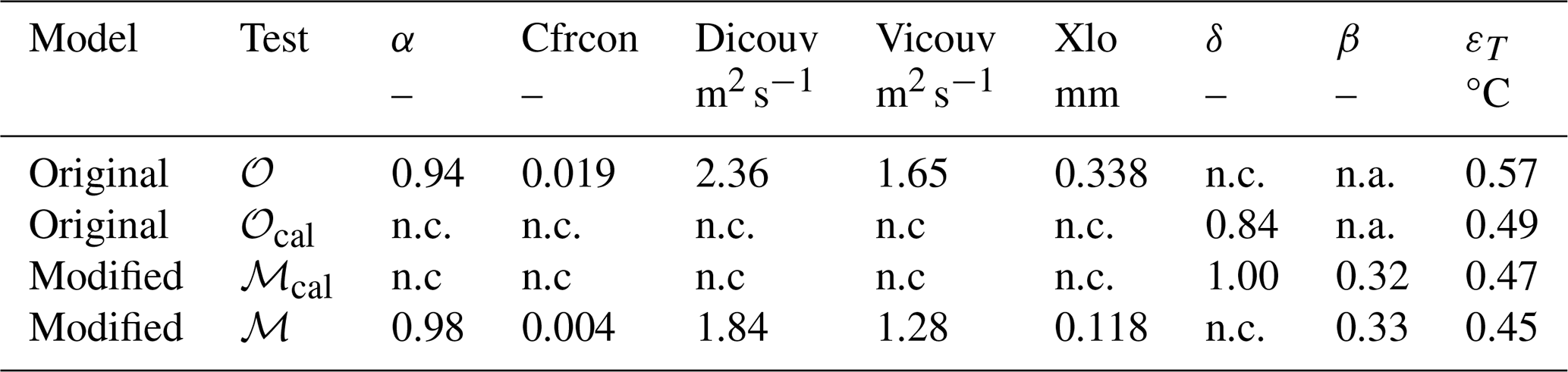
Table 1 Calibration test setups with values of the main parameters (wind drag corrective coefficient (α), free convection coefficient (Cfrcon), horizontal eddy diffusivity and viscosity coefficients (Dicouv, Vicouv), Ozmidov length scale (Xlo), scaling of Secchi depth (δ), and fraction of short-wave solar radiation absorbed in the first layer (β)). 𝒪 identifies the original Delft3D model, while ℳ identifies the modified version including β. Numbers are reported only when calibrated in the test, and “n.c.” stands for “not calibrated”. For the ℳ_cal test, not calibrated parameters are the same as in 𝒪. “n.a.” stands for “not applicable” and only refers to the β parameter which does not exist in the 𝒪 model version.

4 Results

4.1 Base setup model

In this section, we present the results of the calibration of the original model 𝒪 (without β; see Table 1) and without any modification of the Secchi depth. This setup implicitly corresponds to β=0 and δ=1. Figure 2a shows the heat balance terms computed on an hourly timescale at the lake–atmosphere interface on a summer day (17 July 2019), for which in situ measurements of water temperature are available. As expected from the theoretical considerations in Sect. 2.2, the net heat flux is heavily affected by the short-wave solar radiation H_sw0, which however vanishes at night, producing a strong sub-daily variability that is extremely large compared to the other terms. Moreover, if short-wave radiation is excluded from the overall balance H_net, the resulting net heat flux accounting only for the non-penetrative terms (H_np, dashed line) is also negative during daylight hours.

By using the heat fluxes internally computed in the calibrated Delft3D model, we estimated the local warming rate of the surface layer according to Eq. (14), i.e., neglecting advection and diffusion. In this simplified scheme, the heat flux at the surface resulted in an almost always negative value, indicating a predominant heat loss term in the heat equation of the surface layer. As shown in Fig. 2b, where the warming rate σ is plotted everyday at noon, this happens even in the warming periods (spring–summer), with a few exceptions during extremely calm (i.e., low wind) and sunny days. In layers beneath the surface, σ (estimated locally with Eq. 15) instead has a positive sign. In fact, short-wave radiation penetrates the water column with a decreasing warming rate as depth approaches the Secchi depth D_s. Hence, excluding advective and diffusive terms from the simulation, as in Eq. (11), would result in continuous cooling of the surface layer and slight warming of deeper layers. Although this is not the case in the Delft3D model, which accounts for advective and diffusive fluxes, the tendency can also be noted in the numerical results, as will be shown below (Fig. 4).

4.2 Optimal scaling of Secchi depth

The results of the calibration tests 𝒪_cal and ℳ_cal to assess the optimal scaling of the Secchi depth are reported in Table 2. The search for the optimal value of δ depends on the objective function used in the calibration tests.

If the calibration target is the surface water temperature (${\mathit{\epsilon }}_{T_{\mathrm{0}}}$ in Eq. 17) in the original model 𝒪_cal (Fig. 3a–b), the optimal scaling for the Secchi depth unrealistically converges to δ=0.12. Smaller values of δ lead to warmer surface temperature because γ becomes very large (low transparency; see Eq. 2) and because a large portion of the short-wave solar radiation is absorbed in the top surface layer. If the target is the temperature of the water throughout the water column (ε_T in Eq. 16), the optimal value is δ=0.84.

The same plots from the tests ℳ_cal (Fig. 3d–f) suggest that the water temperature can be simulated without the need to drastically minimize δ. The optimal δ converges to 0.57 and 1 for the two objective functions ${\mathit{\epsilon }}_{T_{\mathrm{0}}}$ and ε_T, respectively. The first value (0.57) will be commented on in the Discussion section. Interestingly, Fig. 3e–f show that the value of β converges in a physically meaningful range, and the optimal value is 0.32 for both objective functions (Table 2), fully consistent with the range of literature values (20 %–60 %) presented in Sect. 2.1.

Table 2 Calibrated parameters δ and β and corresponding objective functions. “n.a.” stands for “not applicable”.

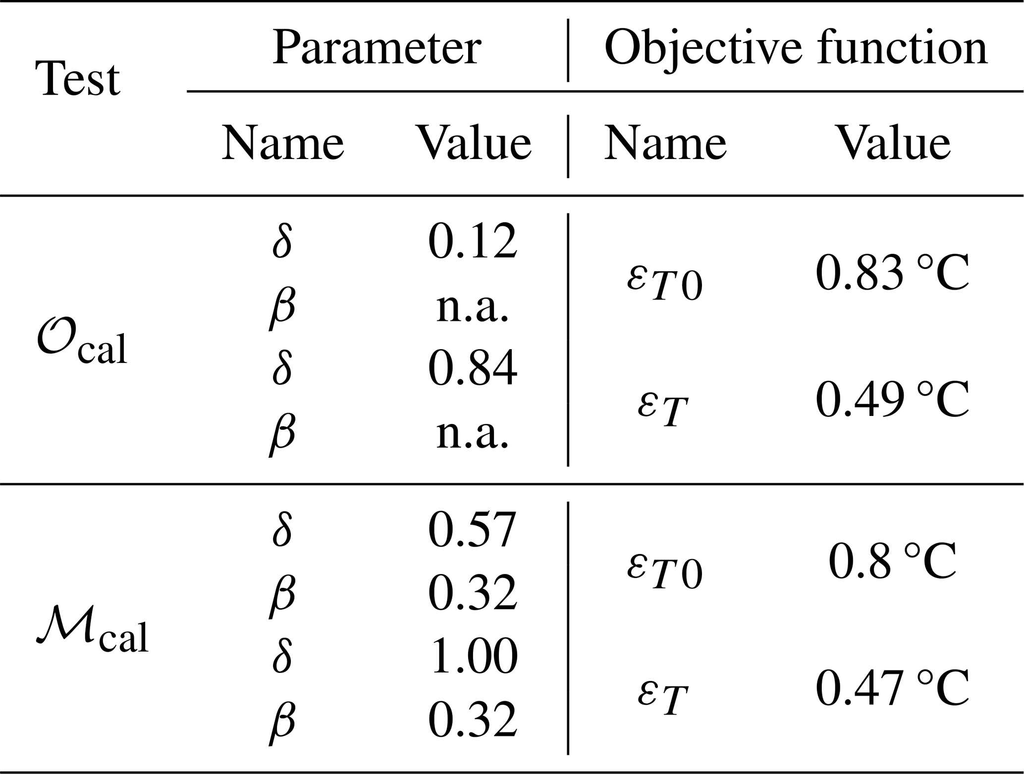
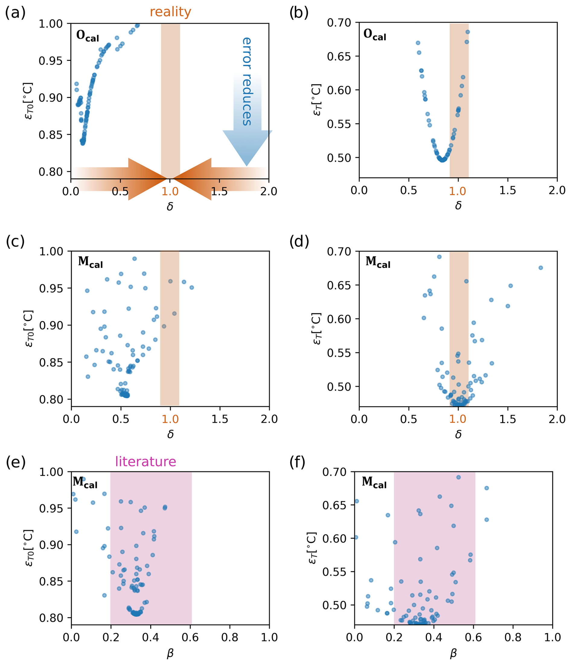
Figure 3 Convergence of different calibration tests and objective functions (a, c, e: ${\mathit{\epsilon }}_{T_{\mathrm{0}}}$, error in surface temperature; b, d, f: ε_T, error in temperature along the water column). (a)–(b) Calibration test 𝒪_cal for optimal δ in the original model 𝒪 (β implicitly equals 0); (c)–(f) calibration of both δ (c, d) and β (e, f) in ℳ_cal tests with the modified model. The blue and orange arrows in panel (a) show the main expected directions of the optimization problem in the calibration of δ (a–d). The orange shaded rectangle in panels (a)–(d) highlights the range of realistic values of δ, i.e., around 1. The pink shaded rectangle in panels (e)–(f) highlights the range of values reported for β in the literature, i.e., 0.2–0.6.

4.3 Effect of β

To understand what actually changes when the parameter β is introduced in the parametrization of the heat flux, Fig. 4 shows the comparison between the fully calibrated models 𝒪 and ℳ (Table 1). Panels (a) and (b) show the simulated temperature profiles on a sample summer day in the two optimal simulations that minimize ε_T, with and without β. The two thermal profiles appear to be very similar to each other and are both consistent with the measurements. Both simulations correctly capture the thermocline depth and the temperature of the surface well-mixed layer (about 7 m thick). However, in the model 𝒪 (panel a) the temperature of the surface layer (23.27 °C) is slightly colder than that of the layers below (23.35 °C), while the surface in situ temperature (24.15 °C) is the warmest. In contrast, the model with calibrated β, i.e., ℳ (panel b), returns 24.50 °C on the surface.

Although the difference in temperature is relatively small between the two versions of the models, the physics behind such thermal profiles is actually different. In Fig. 4c–e, we compare the eddy diffusivity D_z as simulated by the k–ε model in 𝒪 and ℳ on three selected days. In the original model version, stronger turbulent vertical diffusion is simulated in the epilimnion. The largest difference is visible during daylight hours, when the model 𝒪 (panel c) simulates homogeneous diffusivity of the order of 10⁻⁴ m² s⁻¹ in the upper 2 m, while surface mixing is strongly inhibited in the model ℳ (panel d), with D_z generally lower than 10⁻⁶ m² s⁻¹. Thus, the enhanced mixing in the epilimnion simulated by the model 𝒪 compensates for the unrealistic distribution of the warming rate caused by the absence of β, which would produce cooling of the surface layer (as Fig. 2a shows). This effect is visible throughout the simulated period (panel e), with an overestimation of D_z of the order of 10⁻⁴ m² s⁻¹ during daylight hours and higher differences during the stratified period.

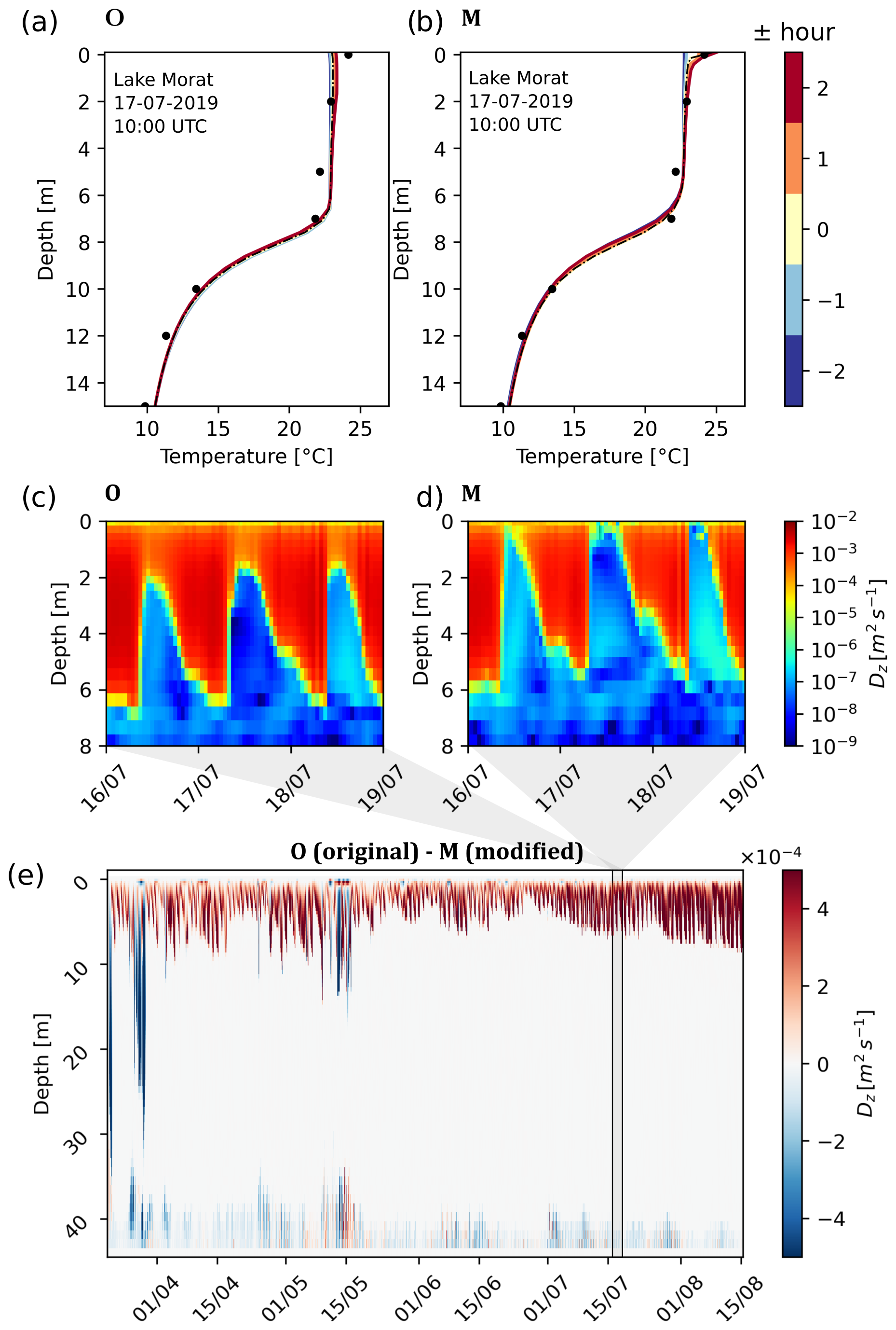
Figure 4 (a)–(b) Temperature profiles simulated (lines) and measured (black dots) on a summer day (17 July 2019) in Lake Morat, implementing the 𝒪 and ℳ model configurations with target ε_T. Model results are displayed at the measurement time (10:00 UTC, black dashed line) and in a time range of ± 2 h around 10:00 UTC. (c)–(d) Vertical eddy diffusivity simulated in the two model setups as in (a)–(b) ± 2 d around 17 July 2019 (black straight line in panel e). (e) Difference in simulated eddy diffusivity between the two models shown on an hourly basis.

5 Discussion

The comparison between the model outputs obtained with the original (𝒪) and modified (ℳ) versions of Delft3D clearly highlights that accounting for short-wave absorption in a shallow layer close to the water surface improves the performance of the model and, more importantly, provides a more realistic description of the physical processes driving surface warming in lakes. The best value of the scaling parameter δ obtained with the modified model is 1 (see Table 1), which implies that the measured value of the Secchi depth in Lake Morat is a reliable input parameter for the model and does not necessarily require calibration. The fact that the measured Secchi depth can be assumed as a physically measurable quantity is a significant advantage in the model setup compared to the common expectation of several Delft3D users that the Secchi depth must be calibrated (Wahl and Peeters, 2014; Soulignac et al., 2017; Piccioni et al., 2021; Xia et al., 2021).

Systematic calibration of model parameters, including Secchi depth, is essential not only for more accurately representing the physics of the system, but also for addressing the imperfections inherent in the model (e.g., neglected baroclinic mixing, imperfect turbulent schemes, unaccounted effects of tributary intrusions, inaccurate atmospheric forcing). Among all the calibration parameters, the Secchi depth is perhaps the most frequently monitored and is one of the easiest to measure, both in situ and through remote sensing. However, several previous modeling studies have highlighted significant deviations of this parameter in Delft3D from the measured values. Here, we demonstrate that this discrepancy is due to a mis-implementation of certain physical phenomena in the Delft3D model, which is supported by the deviation of calibrated Secchi depths after correcting for it. However, there may still be a need to calibrate Secchi depth to account for potential errors in measurements or the sparse resolution of Secchi depth data in both time and space. Meanwhile, calibration of other parameters (e.g., wind drag, background eddy coefficients) will remain necessary to compensate for unresolved processes in the model. We believe that it is good modeling practice to avoid compensating for inaccuracies in one process by adjusting the parameters of others. We therefore suggest focusing on improving model deficiencies and promoting the correct use of parameters to ensure more reliable and physically sound results.

To what extent the modification of the heat fluxes scheme was necessary to improve the performance of the model can be discussed based on the objective functions reported in Tables 1 and 2. Our results indicate that the base calibration of the original model 𝒪 (Table 1) already gives satisfactory results, with an error ε_T=0.57 °C along the water column. This result is possible due to the automated calibration, which allows us to explore a wider range of parameter combinations compared to the manual procedure. The relatively low error also confirms the general reliability of the model with its original formulation, as demonstrated by the numerous successful lake applications in different lakes (e.g., Amadori et al., 2021; Baracchini et al., 2020a; Soulignac et al., 2017, 2018; Wahl and Peeters, 2014; Chanudet et al., 2012; Dissanayake et al., 2019, among many others). By rescaling D_s (i.e., by calibrating δ in the 𝒪_cal test), the error reduced to 0.49 °C. This result is in line with the observations of Amadori et al. (2020) and Piccolroaz et al. (2019), who reduced the measured Secchi depth to improve the performance of the original Delft3D model in Lake Garda. An improvement of 0.08 °C in the model error along the water column is considerable (14 %), but it is achieved at the expense of the physical meaning of the Secchi depth information. If β is introduced and calibrated (ℳ_cal test), we see that the final error ε_T=0.47 °C is only slightly smaller than in the previous case, but a significant gain is obtained in the physical consistency of all inputs (δ=1.0, β=0.32). The value of β estimated by automatic calibration falls conveniently within the range $\mathit{\beta }\in (\mathrm{0.2},\mathrm{0.6})$ observed in different lake environments (e.g., 0.4 in Dake and Harleman, 1969) and suggested in previous modeling applications (Thiery et al., 2014; Cole and Wells, 2015; Schmid and Köster, 2016).

The interesting element of our analysis is that the parameter calibration allows the original model to get close to reality despite the faulty parametrization of the heat absorption at the surface. However, the price of such an optimization is the alteration of other physical processes that compensate for the flaw in the model formulation. This is evident from the enhanced diffusivity at the surface in the original model formulation (Fig. 4), which derived from an unrealistic instability between the upper layer and those below due to surface cooling. This overestimation of surface mixing was also observed by Biemond et al. (2021), who compared the results of the Delft3D model in Lake Garda with in situ turbulent kinetic energy dissipation profiles. In particular, such overestimation was stronger in stratified conditions and was also present when temperature profiles were appropriately simulated.

We have shown in Fig. 4 that the largest difference between the two model configurations is at the surface, particularly during daylight hours in the stratified period. In the temperature profiles shown, a strong gradient is present between the near-surface temperature (i.e., 0 m) and the layer immediately below (2 m). On other days, when the measured surface temperature is relatively well mixed with the layers below, the difference between the two model versions is not that relevant. In fact, if enough mixing is physically provided by, for example, strong wind-induced turbulence, the model does not need to generate artificial convection to compensate for the negative buoyancy at the surface caused by the incorrect parametrization.

The thickness of the model layers also plays a role in the optimal scaling of δ. When the surface water temperature is the calibration target (${\mathit{\epsilon }}_{T_{\mathrm{0}}}$ as an objective function), the optimal value of δ is 0.57 (Fig. 3c), even if β is included in the parametrization and is calibrated. Although 0.57 is definitely more acceptable than 0.12, which was obtained in the case without β (Fig. 3a), it is still significantly smaller than the desirable value, i.e., δ=1. We speculate that this behavior can be interpreted by recalling that the layer in which the β fraction is absorbed is generally considered to be ∼60 cm thick (Henderson-Sellers, 1986). This thickness is used by several models as the reference depth where the exponential decay starts (Zaneveld and Spinrad, 1980; Piccolroaz et al., 2024). Since the thickness of the surface layer in our model is 0.26 m (Table B1), it is possible that the value of δ lower than 1 again compensates for trapping the fraction β in a layer that is too thin. It is therefore likely that if we used a thicker surface layer (e.g., 60 cm thick), the value of the parameter would be closer to 1.

Using automated tools to identify existing flaws could also help improve the representation of other simulated processes. For instance, the impact of density stratification on vertical turbulent fluxes is poorly represented in turbulent schemes, and internal wave breaking is accounted for in only a few lake models, e.g., SimStrat by Goudsmit et al. (2002). Models like k–ε could benefit from supervised automated calibration of parameters that are traditionally fixed based on standard experiments and generally poorly understood. Similarly, refining horizontal turbulent models through tuning could provide insights into whether the adopted scheme (e.g., constant coefficients or sub-grid scaling following  Smagorinsky, 1963) and grid resolution are sufficient to capture the timing and location of horizontal and vertical transport processes, such as upwellings/downwellings and gyres.

6 Conclusions

Automatic calibration tools are powerful for optimizing parameter selection in complex models, helping modelers achieve realistic simulations of the environment studied. Here, we demonstrated that such tools can also be utilized by developers to assess whether their implementations of models align with the physics and by users to identify potential improvements needed in the modeling framework. Unlike manual calibration, which is often user-sensitive and prone to bias, automatic calibration is objective and allows one to more effectively highlight inherent flaws in model formulations. Although lake modeling issues often arise from inadequate meteorological input, automatic calibration can help users and developers detect code-related issues, offering a more unbiased and systematic approach. We tested the response of a hydrodynamic model, Delft3D, which is widely used by the limnological community, to the task of simulating the vertical distribution of heat in lakes. The process is regulated by the well-known Beer law describing the absorption rate of short-wave radiation along the water column, but its incomplete implementation in the numerical model requires a compensation mechanism to optimally simulate surface water temperature. Such a mechanism is the nonphysical adjustment of the Secchi depth to compensate for the exclusion of the absorption of a fraction of solar short-wave radiation at the surface. By exploiting a recently developed calibration tool (DYNO-PODS), based on surrogate models, we were able to unveil such a limitation of the Delft3D parametrization that was never explicitly discussed and to fix it with a small modification of the source code.

In conclusion, we recommend caution when blindly applying automatic tools, emphasizing the importance of evaluating the physical significance of the calibration parameters obtained. This calibration approach combined with detailed analysis of optimization results should yield comparable benefits in various applications, including computationally intensive simulations.

Appendix A: Source code

We report here the parts of the Delft3D code which were modified to include the effect of β according to Eq. (3). Such modification is made in the subroutine heatu.f90.

At the surface layer, the original source code lists the following:

qink  = corr * qsn * (1.0_fp
- exp(extinc*zdown)) / extinc

We modified it as the following:

qink  = corr * (1.0_fp-beta_sw)
*qsn * (1.0_fp - exp(extinc*zdown))
/ extinc
+ qsn * beta_sw

At deeper layers, the original source code lists the following:

qink  = corr * qsn * (exp(extinc*ztop)
- exp(extinc*zdown))

We modified it as the following:

qink  = corr * (1.0_fp-beta_sw)
* qsn * (exp(extinc*ztop)
- exp(extinc*zdown))

Appendix B: Test site and base model calibration

Lake Morat (Lake Murten in German) (Fig. B1a, b) is a Swiss lake situated at 429 m above sea level with a surface area of 22.8 km², an average depth of 24 m, and a maximum depth of 45 m. In situ water temperature profiles are sampled monthly in the middle of the lake (Fig. B1b, c) over irregular depth intervals: 0 (just below the surface), 2, 5, 7, 10, 12, 15, 17, 20, 25, 30, 35, 40, and 43 m. Monthly measurements of water transparency (expressed as Secchi depth, Fig. B1d) are also recorded at the same observation point.

Table B1 Base setup for the Delft3D model of Lake Morat.

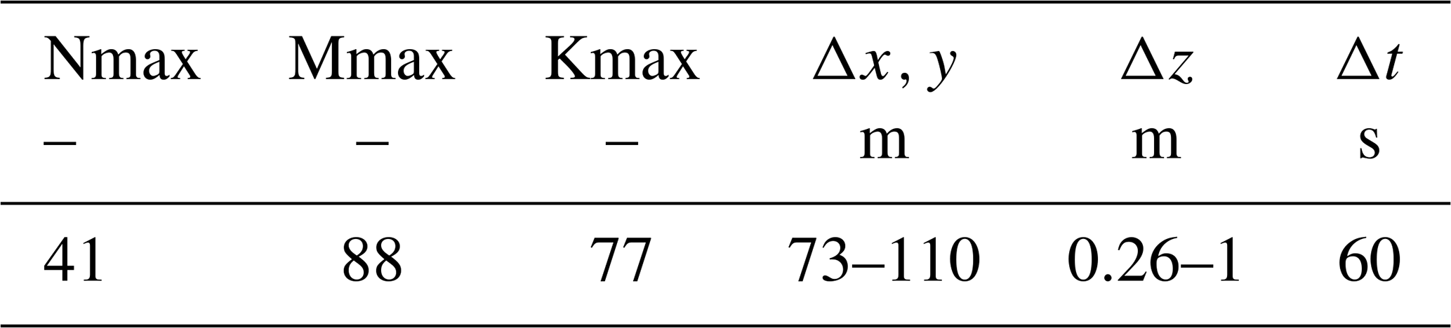
The details on the size of the model grid and the time spacing of the Delft3D model for this lake are reported in Table B1. As atmospheric forcing at the surface boundary of the lake, we used COSMO-1 space- and time-varying meteorological variables (air temperature, relative humidity, wind speed, cloud cover, short-wave radiation, and air pressure), provided by MeteoSwiss at hourly time resolution and 1.1 km spatial resolution. The assimilated outputs, i.e., reanalysis data, based on observational measurements (Voudouri et al., 2017) were used for this purpose.

The base setup for this lake model was obtained from a year-long automated calibration implementing DYNO-PODS (Xia et al., 2022). The full set of parameters are reported in Table 1 in the main text and include the background horizontal viscosity and diffusivity coefficients (indicated as Vicouv and Dicouv in Delft3D; see Deltares, 2023), the Ozmidov length scale (Xlo), the free convection coefficient (Cfrcon), and a corrective coefficient on wind drag coefficient (α). For the wind drag coefficient, as in recent applications of the Delft3D model to peri-alpine lakes (e.g., Amadori et al., 2021), we took as a reference the parametrization proposed by Wüest and Lorke (2003) to set the coefficients of the piecewise function implemented in Delft3D: $C_{dA}^{\mathrm{0}}=\mathrm{0.0044}$ for wind speed lower than U_A=0.5 m s⁻¹, $C_{dC}^{\mathrm{0}}=\mathrm{0.002}$ for values higher than U_C=10 m s⁻¹, and linear interpolations between $C_{dB}^{\mathrm{0}}=\mathrm{0.001}$ and $C_{dA}^{\mathrm{0}}$ and $C_{dC}^{\mathrm{0}}$, respectively, for wind speed between U_B=4.5 m s⁻¹ and U_A and U_C. The wind effect is also taken into account in the parametrization of forced latent and sensitive heat fluxes. Instead of calibrating parameters like the “Stanton” and “Dalton” numbers, respectively, for the sensible and latent heat fluxes (Deltares, 2023), we set the model to also use C_d in calculating these heat fluxes.

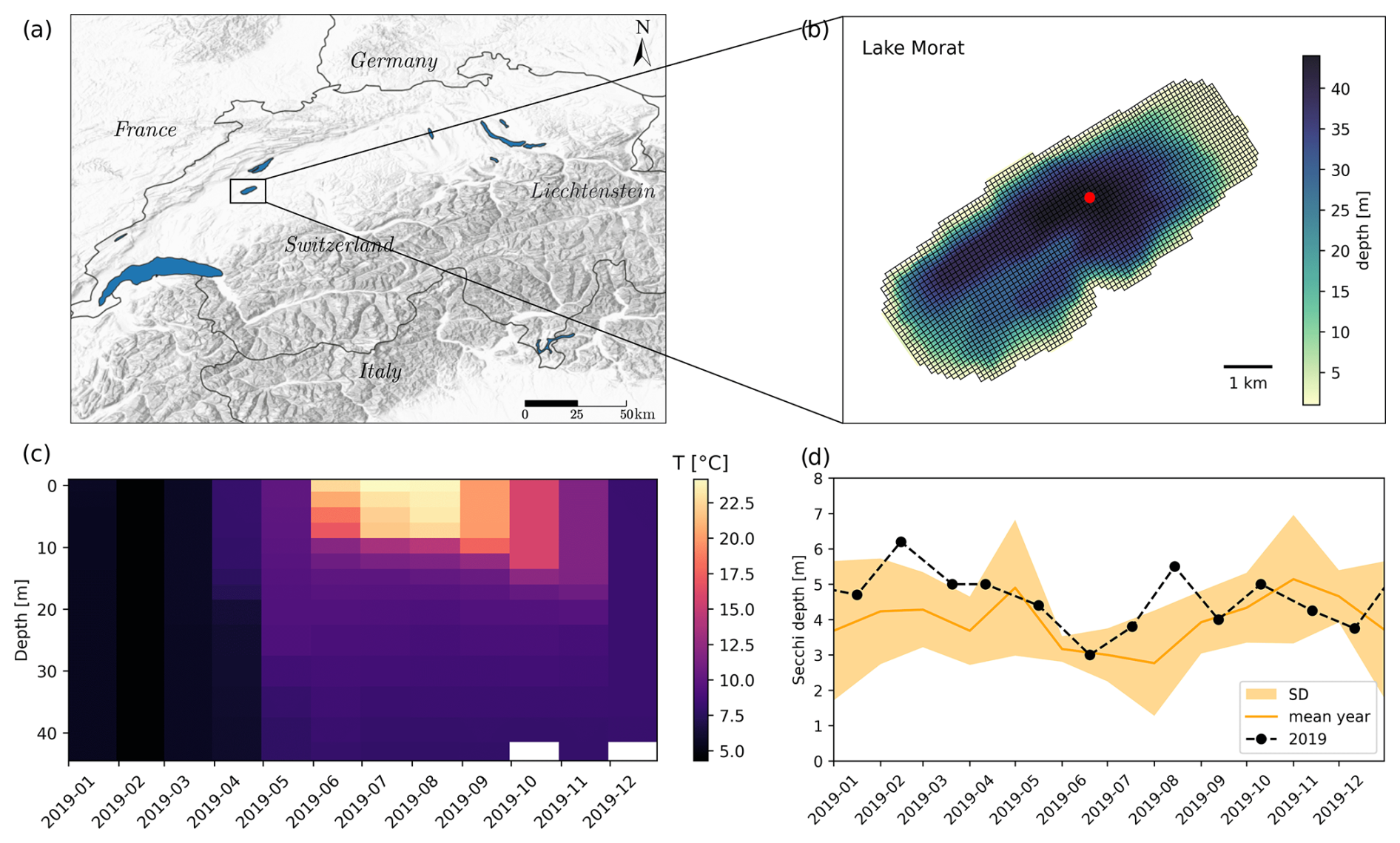
Figure B1 (a) Location of Lake Morat in the alpine area; (b) computational grid, bathymetry, and location of in situ monitoring station (red dot); (c) heatmap of the monthly in situ water temperature profiles for the year 2019 measured in the monitoring point; (d) time series of in situ water transparency for 2019 (black dots) and mean year computed from the 2016–2021 time series (mean: orange thick line; standard deviation: orange shaded area).

To account for the uncertainties related to the input wind speed and to calibrate the wind function for the forced heat fluxes, the drag coefficient was adjusted by introducing the corrective parameter α as follows:

$$\begin{array}{}\text{(B1)}& C_{di}=\mathit{\alpha }{C}_{di}^{\mathrm{0}}.\end{array}$$

Background values of the vertical eddy viscosity and diffusivity (Vicoww, Dicoww ) were set as equal to molecular values (i.e., 10⁻⁶ and 10⁻⁹ m² s⁻¹, respectively), while all the other calibration parameters (e.g., bottom roughness) were set as default values.

The Secchi depth D_s was provided as time series with approximately monthly frequency, as obtained from in situ measurements. These values were not modified. As the objective function for this base calibration, we used the error along the entire water column ε_T.