the Creative Commons Attribution 4.0 License.
the Creative Commons Attribution 4.0 License.
 | 13 Jun 2025
RiverBedDynamics v1.0: a Landlab component for computing two-dimensional sediment transport and river bed evolution
Samuel R. Anderson
Nicole M. Gasparini
Elowyn M. Yager
Computational landscape evolution models (LEMs) typically comprise at least two interacting components: a flow hydraulic solver that routes water across a landscape and a fluvial geomorphological model that modifies terrain properties, primarily bed surface elevation. LEMs used in long-term simulations over large watersheds, including some available in the Landlab library, often assume that only erosive processes occur in rivers and that terrain elevation increases solely due to tectonic uplift. Consequently, these models cannot capture the dynamics of gravel-bedded rivers, lacking the capacity to include sediment mixtures, simulate sediment deposition, and track textural changes in substrate stratigraphy that result from varying flow characteristics. To address this limitation, we developed, implemented, and tested RiverBedDynamics, a new Landlab component that simulates the evolution of bed surface elevation and grain size distribution in 2D grids based on the Exner equation for sediment mass balance. By dynamically coupling RiverBedDynamics with Landlab's hydrodynamic flow solver, OverlandFlow, we created a new LEM capable of simulating the dynamics of local shear stresses, bed load transport rates, and grain size distributions. Comparisons of our LEM results with analytical and previously reported solutions demonstrate its ability to accurately predict time-varying local changes in bed surface elevation, including erosion and deposition, as well as grain size distribution. Furthermore, application of our LEM to a synthetic watershed illustrates how spatially variable rainfall intensity leads to varying discharge patterns, which in turn drive changes in bed elevation and grain size distribution across the domain. This approach provides a more comprehensive representation of the complex interactions between flow dynamics and sediment transport in gravel-bedded rivers at timescales ranging from individual flood events to yearly morphological changes, enhancing our ability to model landscape evolution across diverse geomorphic settings.
- Article
(4492 KB) - Full-text XML
- BibTeX
- EndNote


Landscape evolution models (LEMs) are fundamental tools for geomorphologists, allowing researchers to understand landscape morphology produced under different climatic and tectonic circumstances and, in some cases, informing management decisions (Coulthard, 2001). These models simulate the long-term development of landscapes by incorporating multiple geomorphic processes, providing insights into how terrains change over time under various environmental conditions.
To achieve this, currently available LEMs differ in the number of physical processes considered, the way they route water and sediment across a landscape, and how the domain and its features are represented when solving the governing equations (Coulthard, 2001; Temme et al., 2017; Tucker and Hancock, 2010).
While many LEMs have contributed significantly to our understanding of landscape evolution, they often rely on simplifications that limit their applicability to certain geomorphic contexts. When designed to simulate long time periods, these models incorporate significant assumptions to make computations feasible. These simplifications often include assumptions of steady-state flow, omission of grain size variations and – in many cases – exclusion of sediment deposition processes. A common assumption is that erosive river processes and tectonic uplift are the primary factors shaping a landscape over long timescales (Campforts et al., 2017; Forte et al., 2016; Langston and Tucker, 2018; Li et al., 2018; Whipple et al., 2017). For instance, one of the earlier LEMs, GOLEM (Tucker and Slingerland, 1994), assumed a steady single flow direction with water discharge defined as the product of drainage area and rainfall rate. This approach is still common in LEMs because it greatly simplifies calculations (e.g., Braun and Willett, 2013; Campforts et al., 2017; Goren et al., 2014; Mitchell and Forte, 2023; Tucker et al., 2001). In contrast, CAESAR (Coulthard et al., 2002) employs a routing scanning algorithm that allows multiple flow directions and incorporates flow variability, which enables the simulation of non-steady-state flow conditions and flood wave routing.
To address these limitations, more recent frameworks have focused on advancing sediment transport and deposition modeling capabilities. For instance, CIDRE (Carretier et al., 2023) employs a Lagrangian framework with size-dependent sediment deposition probability, while River.lab (Davy et al., 2017) implements an Eulerian approach. Le Minor et al. (2022) further enhanced these capabilities through improved deposition modeling approaches. While these frameworks have successfully captured key aspects of sediment transport and deposition, they lack the flexibility and comprehensive grain size tracking capabilities that we introduce with RiverBedDynamics. Our component offers unique advantages through its seamless integration with the Landlab platform, allowing easy coupling with any flow solver, and its comprehensive tracking of temporal grain size distribution evolution.
The evolution of landscape modeling frameworks, from earlier LEMs to recent sediment transport solutions, highlights fundamental challenges in simulating river systems across different spatial and temporal scales. In terms of representing drainage networks and channels within a catchment, LEMs employ various strategies to address the challenge of scale. This is crucial because the model grid resolution significantly impacts how different landscape features – such as channels, floodplains, and hillslopes – are represented and captured by the model and, consequently, how governing equations are solved. For example, the CHILD model (Tucker et al., 2001) uses an adaptive triangulated irregular mesh to accurately capture transitions between different landscape elements, particularly the boundaries between channels and floodplains. This approach allows for a more detailed representation of channel networks, a characteristic that is not achievable when using uniform rectangular grid elements. In contrast, CAESAR employs a finer grid resolution near and within channels, especially at their boundaries, to capture the different elements. This method effectively concentrates computational resources where they are most needed for precise flow and sediment transport calculations. The choice of model complexity and resolution has significant implications for the timescales over which LEMs can operate effectively. Simpler models with more assumptions can simulate geomorphological changes over millennia to millions of years with relatively short computation times but at the cost of reduced accuracy and precision. On the other hand, more detailed models, like SedFoam (Cheng et al., 2017), can predict small-scale phenomena, such as sand concentrations in the water column at a sub-millimeter scale, but are computationally expensive and typically limited to shorter timescales and smaller spatial extents.
Beyond considerations of scale and resolution, a critical challenge in landscape evolution modeling is accurately representing the physical processes in gravel-bedded rivers. Current LEMs have been particularly successful in modeling bedrock channels, where the rate of sediment removal is limited by the detachment of material from the bed (detachment-limited conditions). However, this simplification is not adequate when applied to gravel-bedded rivers, where the rate of sediment transport is limited by the flow's capacity to move sediment (transport-limited conditions) (e.g., Attal et al., 2011; Gasparini et al., 2004; Whipple and Tucker, 2002). The evolution of alluvial channel geometries in gravel-bed rivers depends on both erosion and deposition, processes intricately linked to grain size distributions and their evolution over time. Very few LEMs include explicit treatment of grain sizes, yet this factor is critical for both accurately simulating sediment transport and channel morphodynamics and understanding the formation of fluvial deposits. The ability to track grain size evolution is essential for modeling realistic sediment transport rates while also enabling investigation of stratigraphic development and preservation in river systems. Moreover, linking grain size distributions with hydrograph variations is key to modeling realistic shear stress values and provides insights into both the immediate channel response and the longer-term depositional record.
Incorporating deposition alongside erosion in LEMs as a mass conservation problem introduces additional complexity to model development. This approach requires conducting a mass balance at individual cells or control volumes, significantly increasing the computational demands of the model. Thus, LEMs that have adapted a mass balance approach have generally relied on simplified hydrology (e.g., Attal et al., 2011; Gasparini et al., 2004; Whipple and Tucker, 2002). These studies prioritize large-scale trends over long timescales, rather than exploring detailed bed evolution. However, accurately modeling erosion and deposition of different grain sizes remains crucial for understanding gravel-bed river dynamics. This requires a more accurate representation of flow velocity and depth, as these variables are used for calculating sediment transport capacity and determining whether deposition or erosion occurs at any given location.
The need for new models to accurately model grain size distributions presents a significant opportunity for advancing our understanding of landscape evolution, particularly in the context of gravel-bed rivers. Gravel-bed rivers are of paramount importance in geomorphology due to their role in sediment routing, their sensitivity to changes in sediment supply and flow regimes, and their close coupling with hillslope processes. Developing a model that can simulate the evolution of gravel-bed streams in a continuum framework while also linking this evolution to broader landscape processes would represent a major step forward in the field.
To address these modeling challenges, we have developed RiverBedDynamics, a component with a flexible design that operates across various spatial and temporal scales. The component is particularly well suited for analyzing relatively short-term processes (hours to years), where detailed grain-scale interactions and non-steady flow conditions are important. Although theoretically capable of handling longer timescales, the component's mechanistic approach to sediment transport and explicit treatment of flow hydraulics makes it computationally intensive for simulations spanning decades to centuries. The spatial resolution can range from fine-scale process representation (meters) to watershed-scale applications (tens of meters), with users needing to balance tradeoffs between spatial resolution, computational demands, and physical process representation.
This new modeling capability enables researchers to address several important questions in fluvial geomorphology:
- i.
How do variations in sediment supply and grain size distributions influence channel morphodynamics during flood events?
- ii.
What are the feedbacks between bed surface texture evolution and channel adjustment during unsteady flows?
- iii.
How do spatial patterns of erosion and deposition respond to changing climate and land use conditions across watershed scales?
- iv.
What is the role of grain sorting processes in determining channel stability and sediment connectivity through river networks?
- v.
How are climate-driven hydrologic variations preserved in fluvial stratigraphic records, and what can these records tell us about past environmental conditions?
To develop a modeling framework capable of addressing these questions, we leveraged recent advancements in computational platforms. One such framework is Landlab, a Python-based platform designed for creating, assembling, and running 2D landscape evolution models (Barnhart et al., 2020; Hobley et al., 2017). Landlab's modular structure allows researchers to combine various components, each representing different geomorphic processes, to create customized LEMs tailored to specific research questions. Recent efforts within the Landlab framework have made significant strides in improving the accuracy of flow routing and erosion modeling. For instance, Adams et al. (2017) coupled the OverlandFlow component with DetachmentLtdErosion to investigate watershed incision patterns. The OverlandFlow component simulates surface water flow across a landscape, while DetachmentLtdErosion models the erosion of bedrock or cohesive sediment. However, while this approach represents an improvement in flow-routing accuracy, it cannot be directly used in modeling gravel-bedded rivers. The DetachmentLtdErosion component, based on the stream power law, does not account for the complex dynamics of sediment transport and deposition characteristic of gravel-bed systems. Specifically, it does not consider the movement of different grain sizes or the process of sediment deposition, both of which are crucial in gravel-bed river evolution.
An alternative approach within Landlab is the NetworkSedimentTransporter component (Pfeiffer et al., 2020). This Lagrangian model predicts changes in bed material grain size and river bed elevation based on bed load estimates within a predefined river network. It provides valuable insights for long-term simulations of sediment dynamics in established channel networks. While optimized for efficiency in predefined river networks, the NetworkSedimentTransporter was designed with different goals than our component. It operates with a static channel configuration throughout the simulation and focuses on efficient computation rather than tracking stratigraphic evolution or handling unsteady flow conditions. The component was purposefully engineered to process sediment through discrete packets, which offers computational advantages for certain applications. Our RiverBedDynamics component complements this existing work by addressing different research questions, particularly those requiring continuous grain size distributions and dynamic responses to varying hydrological conditions.
The development of these components within Landlab has progressively enhanced our ability to model different aspects of landscape evolution. However, there remains a need for a component that can simulate the full range of processes occurring in gravel-bed rivers while taking advantage of Landlab's integrative framework. While our component primarily addresses sediment transport by flowing water – applying these physics across both channelized and unchannelized areas during overland flow events – other geomorphic processes, such as soil creep, landsliding, and bank erosion, require different physical representations through specialized Landlab components. In particular, the ability to model sediment transport and deposition across varying flow conditions while tracking both spatial and temporal evolution of grain size distributions would represent a significant advance in our modeling capabilities.
These existing components, while valuable, highlight a critical gap in our ability to model gravel-bed rivers within the context of landscape evolution. To address these limitations, a component is required that can (i) accurately represent sediment transport dynamics in gravel-bedded rivers; (ii) account for fractional sediment transport, including erosion and deposition processes; (iii) predict bed surface changes across an entire watershed; and (iv) integrate flow prediction with high accuracy under non-steady and non-uniform conditions.
To address this gap, we developed RiverBedDynamics, a new Landlab component designed to simulate the evolution of gravel-bed streams in a continuum model, allowing for the integration of the channel with other geomorphological processes using the Landlab platform. By coupling RiverBedDynamics with OverlandFlow, we enable the simulation of non-steady flow conditions, which is crucial for understanding the complex dynamics of gravel-bed rivers. The component addresses the limitations of existing models by incorporating grain size evolution, non-steady flow conditions, and watershed-wide predictions of bed surface changes. A key feature of our component is its ability to track and preserve stratigraphic information, enabling investigations of both short-term morphodynamics and longer-term geological processes. This stratigraphy tracking functionality allows researchers to study how temporal variations in flow and sediment transport conditions are recorded in depositional sequences, providing insights into the geological history of river systems.
In this article, we introduce RiverBedDynamics and demonstrate its capabilities in modeling gravel-bed river evolution within a landscape context. Through a series of tests and applications, we illustrate how RiverBedDynamics can capture key aspects (e.g., sediment transport dynamics, grain size evolution, erosion and deposition processes, and watershed-scale bed surface changes) of landscape evolution, particularly in systems dominated by gravel-bed rivers. All sediment transport predictions are based on the unsteady total shear stress, which accounts for spatial and temporal gradients in flow velocity and local variations in bed elevation and water depth. Evaluations of our component are conducted using test cases with analytical solutions from previously available models. An example in a large watershed is used to explore large-scale applications of the component.
Landlab, a Python-based interdisciplinary open-source platform, serves as a robust framework for developing computational landscape models addressing earth surface dynamic processes (Barnhart et al., 2020; Hobley et al., 2017; Tucker et al., 2022). We integrate our component into Landlab, leveraging its seamless support for incorporating new process components. Further, Landlab already contains a simplified hydrodynamic model for computing flow variables, upon which RiverBedDynamics relies (Adams et al., 2017). Numerous studies detail the general structure of Landlab (e.g., Adams et al., 2017; Barnhart et al., 2019, 2020; Hobley et al., 2017; Shobe et al., 2017; Tucker et al., 2022); therefore, we focus here solely on aspects relevant to implementing the RiverBedDynamics component.
At the core of our component lies Landlab's gridding engine, facilitating data manipulation and exchange among various components. This engine operates on a 2D structured grid, enabling numerical operations essential for calculating flow, bed surface changes, and sediment variables during simulations. For instance, the grid contains methods for computing topographic gradients and sediment mass balance and mapping velocities from grid links to nodes. Currently, our component exclusively operates on raster grids (Fig. 1). Within this grid framework, nodes represent discrete (x; y) points, while links denote vectors connecting neighboring nodes with fixed directionality. A cell, bounded by faces, encapsulates the area around a non-perimeter (i.e., interior) node. All cells within our component are rectangular-shaped and maintain uniform dimensions in both the x (Δx) and the y (Δy) directions.
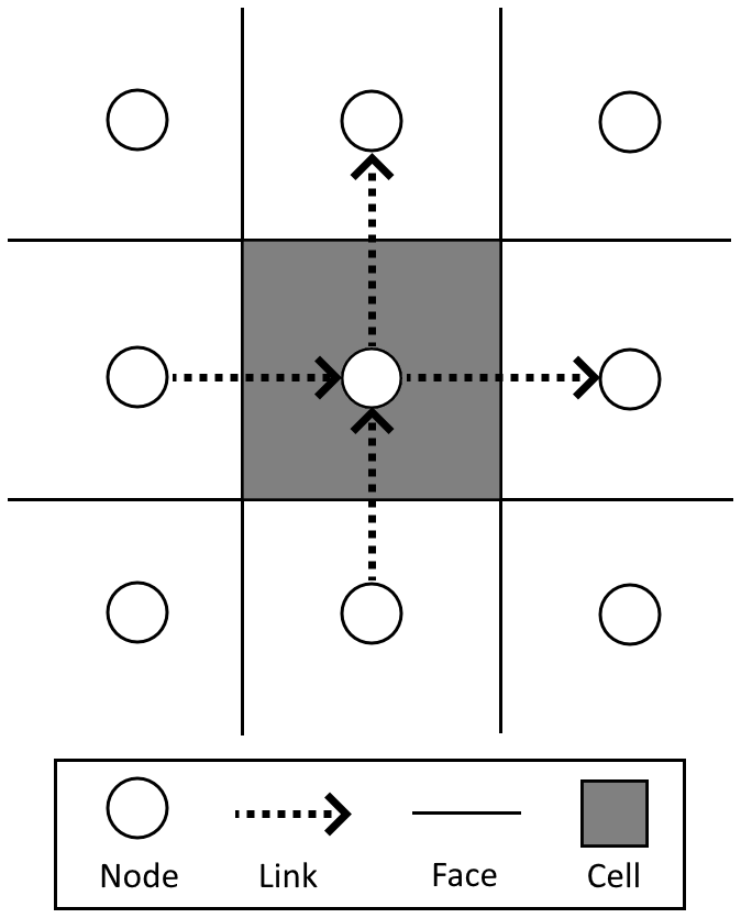
Figure 1Elements of a Landlab grid used by our component, illustrating a typical grid segment. Information is stored in nodes and links. For instance, surface bed elevation data are held at the nodes, whereas the gradients of these elevations are stored in the links.
Our component was developed around the RasterModelGrid class, chosen for its ability to facilitate the numerical solution of partial differential equations, such as the Exner equation for sediment mass conservation, and spatially variable processes in a straightforward manner. For instance, consider the Meyer-Peter and Müller (1948) equation for bed load transport:
where is the dimensionless critical shear stress, is the dimensionless volumetric bed load transport rate per unit width, and τ* is the dimensionless shear stress. Implementation of Eq. (1) requires calculating τ* at each node and determining locations where τ* exceeds to compute . Using Landlab's structure and tools, Eq. (1) can be implemented as
Here, tau_star is extracted from the grid, while tau_star_cr, qb_star_coeff, and qb_star_exp are the equation's parameters (0.047, 8, and , respectively). This implementation illustrates a key advantage of Landlab's design: the ability to translate mathematical equations directly into code that operates efficiently across the entire domain. The similarity between Eq. (1) and its implementation demonstrates how Landlab's grid-based structure eliminates the need for explicit iteration over individual cells, making the code both intuitive and computationally efficient. This direct mapping between mathematics and code is a fundamental feature that extends to all processes implemented in the framework. Additionally, data exchange between different Landlab components is seamlessly facilitated by the grid. For instance, modifications to the bed surface elevation in RiverBedDynamics result in the updated value being immediately available to all Landlab components via the field grid [“node”][“topographic__elevation”].
Boundary conditions in our component are inherited from the Landlab grid object, aligning with those specified in the OverlandFlow component (Adams et al., 2017). Nodes defined as “boundary” can be designated as open, fixed gradient, or closed. Open boundary nodes allow flux to enter or leave the model domain, acting as flow outlets. Closed boundary nodes prevent flux from entering or leaving the domain. This classification determines the behavior of surface water flow at these boundary nodes, with sediment fluxes calculated based on local flow conditions. Links connected to these boundary nodes are automatically classified as active, inactive, or fixed. Active links, where fluxes are calculated, occur between two core nodes or between a core node and an open boundary node. Inactive links, where no fluxes are calculated, occur between a closed boundary node and a core node or between any pair of boundary nodes. Fixed links, which can have assigned values, occur between a fixed gradient node and a core node. The sole exception to these inherited conditions is at the domain outlet. Here, RiverBedDynamics requires specifying either a fixed bed surface elevation or a zero-gradient condition (refer to Sect. 3.4 for more details).
Our component was designed to work in conjunction with a flow solver such that continuous feedback between surface flow and river bed properties determines the behavior of the system. While RiverBedDynamics is compatible with any flow solver through Landlab's “plug-and-play” capabilities, in the examples presented in this paper, we demonstrate its use with the OverlandFlow component (Fig. 2). This specific choice of flow solver illustrates one possible implementation, but users can integrate RiverBedDynamics with other flow-routing components available in Landlab depending on their needs. At each time step, the flow governing equations are solved across the entire domain by OverlandFlow, obtaining flow depth, velocity, and discharge. The routines of RiverBedDynamics can be conceptualized as two major parts: (i) bed load transport and (ii) river bed evolution. In the first part, RiverBedDynamics processes surface flow and bed surface grain size properties stored in the grid to calculate local shear stress and the bed load transport rate. In the second part, it uses sediment fluxes entering and leaving each cell to compute the mass balance. This process updates the bed surface elevation and bed properties, such as grain size distribution, thereby completing the cycle at each time step.
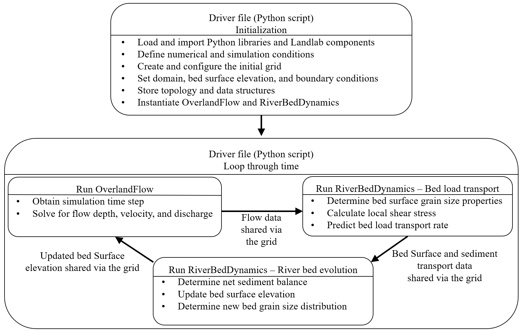
Figure 2Simplified workflow for the coupled OverlandFlow and RiverBedDynamics routine. The driver file is a procedure script containing the set of instructions to create all the required data and loops through time, dynamically linking and updating surface flow and river sediment variables.
3.1 Flow variables and shear stress calculations
During each time step of a simulation, OverlandFlow solves the 2D flow equations across all grid links, determining the surface water discharge per unit width (q), flow velocity components (u and v, corresponding to the x and y directions, respectively), and water depth (h) at links. Subsequently, water depth at nodes is calculated based on mass conservation, factoring in all inflow and outflow at a given node. These spatial distributions of flow variables provide the foundation for subsequent sediment transport calculations. While flow velocity is not directly derived, it can be calculated at links according to with the velocity components u and v for the x and y directions, respectively. Our sediment transport rate calculations are based on the local shear stress considering an unsteady friction slope (Ghimire and Deng, 2011) according to
where u and v are the velocity components in the x and y directions, respectively; Sfx and Sfy are the friction slopes evaluated in the x and y directions, respectively; η is the bed surface elevation; g is the acceleration due to gravity; and t is time. This formulation is an extension used in shear stress calculations of the commonly used depth–slope product, in which steady and uniform flow conditions are assumed, resulting in in the x direction. The unsteady friction slope formulation accounts for both spatial variations in flow properties and their temporal changes, including acceleration and deceleration effects that are particularly important during flood events.
Each individual term in Eq. (2) is calculated directly using built-in methods of the Landlab grids. Topographic gradients ( and ) are based on the bed elevation slope at the nodes defining a link using the calc_grad_at_link method. The same approach is used for water depth spatial gradients ( and ). Velocity spatial gradients are approximated using a central difference scheme according to
where subscripts x+1, x−1, y+1, and y−1 indicate the location of the link considered to the right, to the left, above, and below, respectively (Fig. 3). Velocity time gradients are approximated using the backward Euler method defined as
where Δt is the time step, and the superscripts t and t−1 indicate the current and previous time steps. The velocity at the previous time step (t−1) is stored in the field surface_water__velocity_prev_time_link and is updated at every time step. At the beginning of the simulation, this gradient can be forced to zero or initialized with a known velocity value if available as an initial condition.
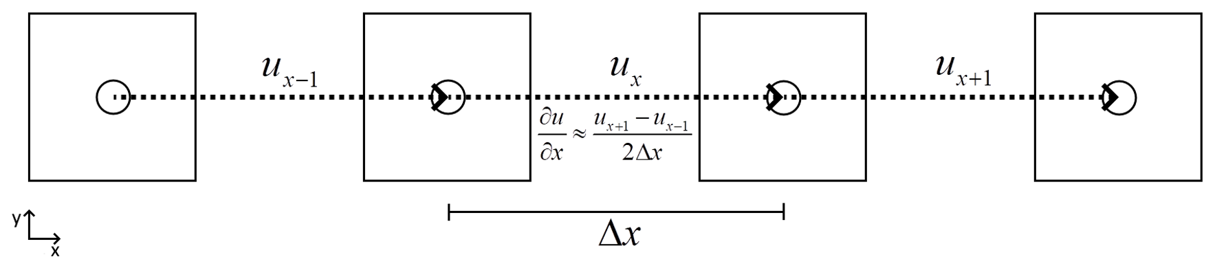
Figure 3A representation of the stencil used to calculate the velocity gradient at links. Cells are separated only to highlight the definition of velocities at links. The gradient at the location of the link with velocity ux is estimated using a central difference scheme and considers the neighboring links. The same principle applies to calculate but is not represented in this figure.
While a two-point scheme, like upwind, provides better numerical stability in advection-dominated flows, we opted for the central difference scheme, primarily because it provides more accurate approximations of spatial gradients (with errors proportional to the square of the grid spacing) compared to first-order schemes like upwind differencing and because of its ability to capture multi-directional information propagation in our coupled system. This choice reflects a balance between computational accuracy and physical representation, which is particularly important when simulating complex watershed-scale processes with varying flow conditions. The scheme's higher-order accuracy and multi-directional nature are especially beneficial for resolving flow dynamics at channel confluences and during rapid flow variations, where information propagates in multiple directions simultaneously.
The local shear stress at each link is then calculated according to
Typically, shear stress in river channels is defined using the hydraulic radius rather than water depth to account for bank roughness. However, the choice between these approaches depends on the spatial resolution relative to channel width and the processes being represented. We use water depth as the default option for calculating shear stress because, (i) when cell sizes are much smaller than channel widths, most cells represent the channel interior and do not contain riverbanks, making the hydraulic radius effectively equivalent to water depth, and (ii) when cell sizes are much larger than channel widths, a single cell contains both the channel and the surrounding floodplain. In this case, most cell boundaries interface with other water-filled cells rather than channel banks, again making hydraulic radius less representative, and (iii) our model simulates both channelized flow and overland flow on hillslopes using the same equations. For overland flow, the concept of hydraulic radius is not applicable due to the absence of channel banks.
The hydraulic radius approach is most appropriate when cell size closely matches channel width, where a significant proportion of the flow surface contacts both the river bed and riverbanks. Since it is difficult to predict this specific case across an entire model domain, we set water depth as the default in shear stress calculations. Nevertheless, users can override this default by setting use_hydraulics_radius_in_shear_stress = True when instantiating the RiverBedDynamics component, which calculates shear stress using
where is the hydraulic radius, Aw=hΔx is the wetted area, and is the wetted perimeter. For north–south links we have Aw=hΔy and .
While our component focuses specifically on sediment transport by flowing water, we acknowledge that other important hillslope processes, such as soil creep and mass wasting, require different treatment. These processes can be represented by coupling RiverBedDynamics with other Landlab components, such as TransportLengthHillslopeDiffuser for soil diffusion and LandslideProbability for mass wasting. Future versions of the model may also incorporate an option to estimate sub-grid channel widths for cases where channels are significantly narrower than grid cells.
3.2 Bed surface properties and sediment flux calculations
Prior to calculating sediment fluxes, RiverBedDynamics determines the bed properties required for the bed load transport equations. During instantiation, bed grain size distributions (GSDs) are specified at nodes, which allows them to vary spatially. Grain sizes, defined as percentage passing, can range from fine sand to large boulders. Cohesive sediments are not supported by our component. For any sediment transport model used, it is mandatory to define the grain sizes at 0 % and 100 % of the distribution. This ensures uniformity in input format across different bed load transport equations.
Once the GSD is specified, the model calculates the following parameters at nodes: sand fraction (Fsand), D50, the geometric mean size (Dsg), and the geometric standard deviation (σg). The last two variables are defined following the method of Parker (1990). After bed properties are defined, they are mapped onto the links assuming that the connecting nodes have equal weights. The selected bed load equation defines whether these bed surface properties are updated at each time step or remain constant throughout the simulation (see below).
Six different sediment transport equations are available in our component. These equations are described in detail in the original articles (Fernandez Luque and Van Beek, 1976; Huang, 2010; Meyer-Peter and Müller, 1948; Parker, 1990; Wilcock and Crowe, 2003; Wong and Parker, 2006) and have been used extensively in sediment transport studies (e.g., Barry et al., 2004; Schneider et al., 2015; Yager et al., 2007). Therefore, only the aspects related to their implementation are described here.
The first group of equations include those by Meyer-Peter and Müller (1948), Fernandez Luque and Van Beek (1976), Wong and Parker (2006), and Huang (2010). We collectively refer to these as Meyer-Peter- and Müller-style equations. They have the following form:
where the coefficient α, the exponent β, and are parameters specific to the selected equation. These equations are only valid when or else . When selecting these equations, the grain size distribution of the bed remains constant during the entire simulation. The dimensionless shear stress is calculated as , where , and ρs and ρ are the densities of the sediment and water, respectively. For simplicity, the x and y subscripts from Eq. (5) are omitted in this and subsequent uses of τ.
The effect of bed slope on critical shear stress (Lamb et al., 2008; Mao et al., 2008; Mueller et al., 2005; Smith et al., 2023; Yager et al., 2012) in relatively steep slopes (larger than 3 %) can be empirically included in Meyer-Peter- and Müller-style equations by setting the option variable_critical_shear_stress = True during instantiation. When activated, the Mueller et al. (2005) equation is used to calculate :
where Sb is the topographic gradient defined as and for the x and y directions, respectively. While this optional setting simplifies the complex processes governing critical shear stress variation with slope, it serves as a practical tool for analyzing the model's response to in terrain slopes exceeding 3 %. We acknowledge that this approach is a generalization, and incorporating the full mechanics of these processes is outside the current scope of RiverBedDynamics.
Another option is the surface-based bed load transport equation of Parker (1990) that includes the effects of sediment mixtures in gravel-bedded rivers but does not include sand size material. In this case, if sand is present in the GSD, the component will automatically remove it and renormalize the GSD curves to adjust for the change. The shear stress is normalized here using Dsg instead of D50 as follows:
The dimensionless measure of shear stress is
where is the reference Shields stress. To account for the effects of sediment mixtures, a hiding function is used:
where the subscript i denotes the ith grain size class. The function ω is
where σ0(ϕsg0) and ω0(ϕsg0) are functions that are calculated automatically within the component. The dimensionless transport rate for each ith size class is defined as
and the function G(ϕi), the normalized dimensionless gravel-bed-load transport rate, is
To obtain the fraction of bed load in each ith size class (pi), we used
where Fi is the volume fraction in the bed of the ith grain size class, and N is the number of grain size classes with characteristic diameters Di.
The last bed load transport equation included in our component is that of Wilcock and Crowe (2003). Similar to Parker's (1990), this model can handle sediment mixtures. However, in this case, the effects of sand content (Fsand) are explicitly included in the reference Shields stress, which is defined as
The dimensionless measure of shear stress is , and the hiding function is expressed as
where the exponent is
The dimensionless transport rate for each ith size class () is
To obtain the fraction of bed load in each ith size class (pi), we used
The volumetric bed load transport rate per unit width for each grain size when using the equations of Parker (1990) or Wilcock and Crowe (2003) is calculated using
Given that we are working in a 2D structured grid, we can assign directionality to qb depending on the link in which it is being calculated, qb,x for east–west, and/or qb,y for north–south links, by multiplying Eq. (21) by the sign of τ. The total bed load transport rate per unit width qb is defined as the sum of the bed load transport rates of each grain size qbi.
3.3 Sediment mass conservation and bed property update
Once the sediment fluxes and bed load GSD at each link are calculated, it is possible to conduct a mass balance at nodes and determine changes in bed surface elevation and bed GSD. Surface bed elevation changes are calculated by the update_bed_elevation routine within RiverBedDynamics using the Exner equation:
where λp is the bed porosity. The equation states that the change in bed elevation in time within a control volume, a cell in this case, is a function of the sediment fluxes crossing the faces of a cell (Fig. 4).
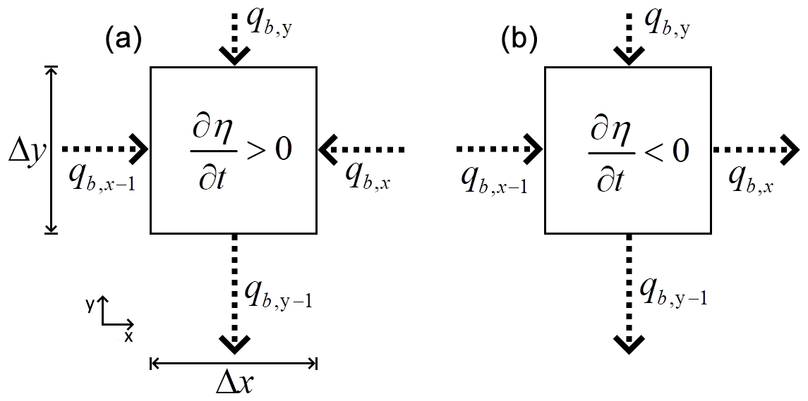
Figure 4Examples of an increasing (a) and decreasing (b) bed surface elevation in time. Arrows indicate the direction of sediment fluxes across cell faces (arrow size adjusted for visibility), with flux directions determining the net bed load transport rate within a cell and consequently dictating erosion or deposition of sediment. In panel (a), the sum of the three fluxes entering the cell is larger than that exiting the cells; therefore, there is a net accumulation of sediment, and the bed elevation increases. In panel (b), fluxes in the x direction are equal in magnitude and cancel each other out, whereas in the y direction, the flux leaving is larger than that entering; consequently, the bed elevation will decrease.
We used an explicit method to approximate the solution of Eq. (22). The gradients in the volumetric bed load transport rate per unit width in the x and y directions are
where the locations x, x−1, y, and y−1 are shown in Fig. 4. The right-hand side of Eq. (22) can be expressed as
Here, Δqb,xΔy and Δqb,yΔx are the volumetric bed load transport rates in each direction, is the net volumetric bed load transport rate, and ΔxΔy=Axy is the area of a cell. Considering these definitions, the explicit solution to Eq. (22) is
The choice of an explicit scheme for solving the Exner equation (Eqs. 22 and 25) was motivated by its simplicity and ease of implementation, particularly when coupled with the OverlandFlow component. While OverlandFlow uses an implicit scheme for flow routing, which is advantageous for maintaining stability in hydrodynamic simulations, the explicit approach for sediment transport allows for straightforward integration of sediment fluxes and bed elevation updates at each time step.
However, the explicit scheme imposes stricter stability constraints compared to implicit methods. The time step (Δt) must satisfy the Courant–Friedrichs–Lewy (CFL) condition for sediment transport, which can be approximated as
This condition ensures that sediment fluxes do not exceed the capacity of the grid cells to accommodate changes in bed elevation within a single time step. In practice, the time step is further constrained by the need to maintain numerical stability in the coupled system, particularly during rapid changes in bed elevation or flow conditions. Our testing shows that time steps of 1–5 s typically maintain stability for spatial resolutions of 25–100 m in watershed applications, though these values should be adjusted based on specific flow and sediment transport conditions. We recommend that users start with small time steps (around 1 s) and gradually increase them while monitoring solution stability.
Boundary conditions for updating the bed surface elevation are only required at the links located immediately upstream of the watershed outlet. Two options can be specified, zero gradient (default) or fixed value. The zero-gradient condition allows the bed elevation at the outlet to evolve naturally based on upstream conditions, maintaining the same bed surface elevation slope as the immediately upstream reach. This approach permits sediment to be transported through the outlet based on local transport capacity, rather than imposing an artificial constraint on sediment flux. The net sediment exchange at boundary cells is identical to that located upstream of the outlet, ensuring sediment flux out of the domain. The fixed-value condition, alternatively, maintains a constant bed elevation at the outlet, which can be useful when modeling systems with known base levels. However, it is important to note that sediment fluxes can be independently specified at any location in the domain, including inlet boundaries, outlet boundaries, and internal nodes and links. This flexible approach allows users to implement various sediment supply scenarios and internal sediment sources or sinks.
In practice, the zero-gradient condition is implemented using user-provided methods for the watershed outlet boundary condition (e.g., set_watershed_boundary_condition_outlet_id, set_watershed_boundary_condition) to identify all connecting nodes and links upstream of the outlet. At the end of the bed elevation update routine, RiverBedDynamics adjusts the bed elevation of outlet nodes to match the upstream slope, maintaining continuity in both elevation and sediment transport. This prevents artificial disruptions to sediment transport at the boundary while ensuring a physically consistent outlet condition. When other types of boundary conditions are required, such as an elevation that changes in time following a given curve, it can be specified by setting individual nodes or links of the grid using Landlab boundary condition handling. Fixed-value conditions can be applied, not only to the boundaries, but also to internal nodes, such that they can remain unaltered throughout the whole simulation. This optional capability is accessed by editing the field “bed_surf__elev_fix_node”.
Sediment mass entering or leaving a cell can alter not only the bed surface elevation but also the bed GSD. We represent the evolution of the surface and substrate GSD by means of three layers (bed load, surface, and substrate; Fig. 5) to capture key physical processes in gravel-bed rivers. This multi-layer approach is essential for accurately modeling (1) the interaction between flow and the active surface layer where sediment exchange occurs; (2) the development of bed-armoring and sorting patterns; and (3) the preservation of depositional history in the substrate, which influences future bed evolution. The bed load layer is the one defined by the bed material being transported close to the river bed and is calculated according to Sect. 3.3. The surface layer, which is in direct contact with the flow at wet nodes, determines the bed surface elevation, measured from a specific datum point (η). It contains the active layer, characterized by a thickness defined as La=2D90 (D90 is the 90th percentile of the surface GSD). The surface layer can exchange material with the bed load or substrate layer depending on whether the bed aggrades or degrades, respectively. We acknowledge that using a constant active-layer depth is a simplification of the physical processes occurring in natural rivers, where the active-layer depth can vary with flow strength and unsteady conditions. This assumption may affect the accuracy of predicted bed–substrate interactions, particularly during high-flow events when the actual active-layer depth might be greater than our specified value. The constant active-layer depth could potentially underestimate the exchange of material between the bed surface and substrate during high flows, limit the model's ability to capture deep-scour events, and affect the predicted rate of bed-armoring and sorting processes. However, this simplification was chosen to maintain computational efficiency and stability in watershed-scale applications. Future versions of the component could incorporate a variable active-layer depth based on flow conditions, though this would require additional validation against field observations. To simplify the definition of the surface layer and facilitate the implementation of its updating algorithm, we adopted the definition of Toro-Escobar et al. (1996), which posits that the surface layer and the active layer are of equal thickness, La (Fig. 5). The substrate includes all the material below the surface layer. Its GSD is represented using Fsi, analogous to the way Fi defines the surface GSD.
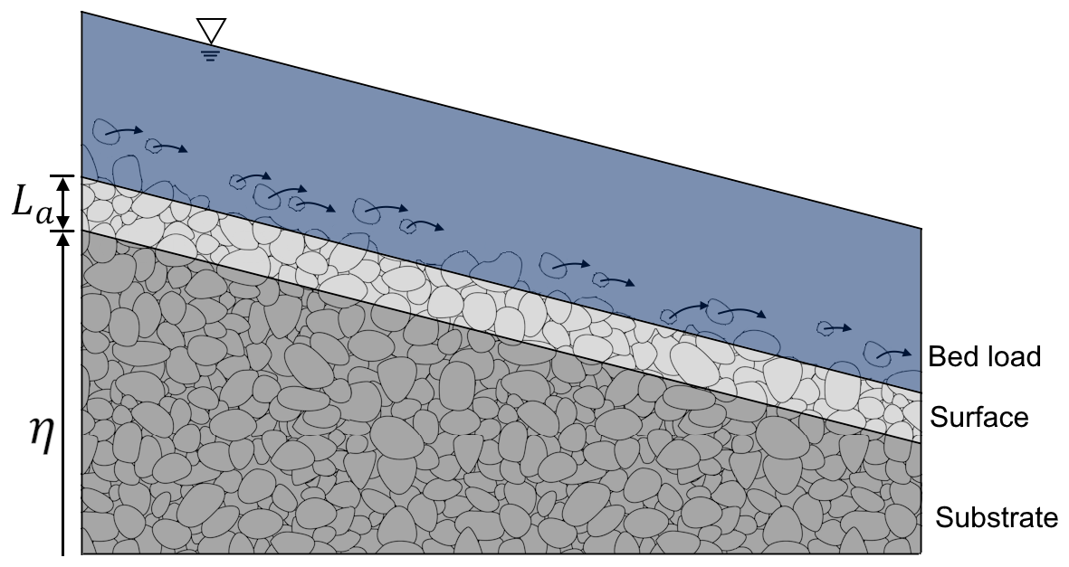
Figure 5Schematic diagram of the model's three layers, used to represent the evolution of the surface and substrate grain size distribution.
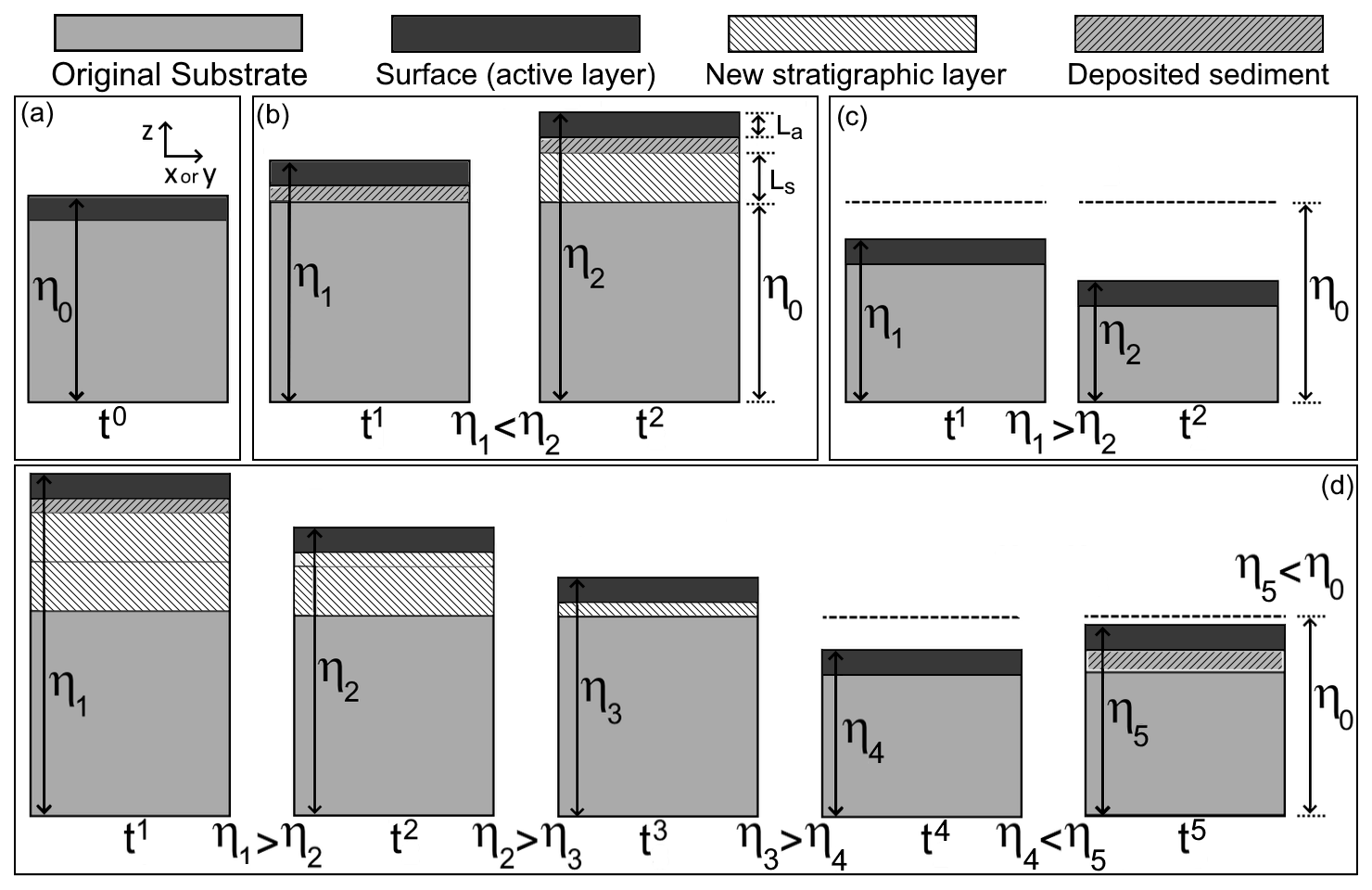
Figure 6Graphical description of the model's algorithm for updating bed surface and substrate GSD. (a) Initial bed surface elevation (η0) at the start of the simulation (t0). (b) A purely depositional process. The bed surface elevation monotonically increases, and new stratigraphic layers form once the deposited layer's thickness reaches Ls. The GSD of the deposited sediment is calculated using Eq. (26). (c) A purely erosional case. Bed surface elevation monotonically decreases, and the surface and substrate have the GSD specified at t0. (d) An alternating erosion–deposition case. The bed is first eroded below the initial elevation (at t4), following the erosion of newly deposited layers (at t1 and t2), and then experiences deposition again (at t5). The local minimum bed surface elevation is updated to η4, and the GSD at η5 is calculated using Eq. (26).
To account for the dynamics of active-layer grain sizes, we implemented the grain-size-specific form of the Exner equation, as described by Parker (1991):
where fIi accounts for the interchange of sediment between the active layer and the substrate interface. This corresponds to the fraction of material in the ith grain size exchanged between these two layers. In our model, we used the transfer function of Toro-Escobar et al. (1996):
This equation states that when the bed degrades, the active-layer GSD is that of the substrate (Fig. 6c). Conversely, when the bed aggrades, a mixture of surface and bed load material transfers to the substrate, thereby creating stratigraphy.
We solved Eq. (26) explicitly by approximating the derivatives as
The y direction has an equivalent discretization (just replacing x with y). The coefficient α is used to switch from an upwind to a central difference scheme. For stability purposes, we opted for a default value of 1. The explicit solution to Eq. (26) is
For simplicity we dropped some t superscripts, but all variables except are evaluated at the current time step.
Given that our model can predict temporal changes in bed surface elevation and GSD, we implemented stratigraphy tracking capabilities, thus allowing a better representation of processes that are not purely erosional or depositional. Our model stores the current and past GSD and elevation of the surface and substrate across the whole watershed (Fig. 6). At the beginning of a simulation, the surface and substrate have, by default, the same GSD (Fig. 6a). When deposition occurs at a given location, RiverBedDynamics stores the elevation and GSD of the deposited sediment; these data are recorded at regular intervals determined by the variable num_cycles_to_process_strat. Once the accumulated deposited material at that location reaches the user-specified vertical thickness (bed_surf_new_layer_thick, default value of 1 m, Ls in Fig. 6b), it is logged as a new layer of stratigraphy. The recorded GSD for this layer is a time-averaged value derived from all the sediment deposited over the last bed_surf_new_layer_thick meters, after which the process begins anew. In scenarios where a new stratigraphic layer is being eroded, the model reads the stored data and adjusts Fs and Fsi based on the elevation of the layer being scoured (Fig. 6d). When the bed surface is eroded below the initial bed surface elevation, Fs retains its original state from the beginning of the simulation (Fig. 6c).
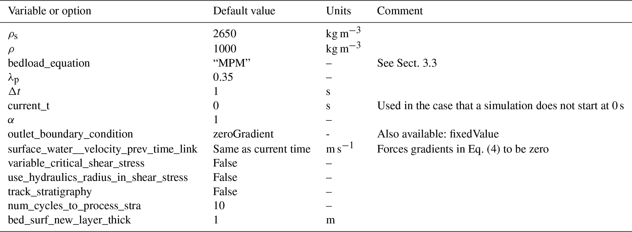
Some general characteristics of the Landlab modeling approach were described in Sect. 2.0. Therefore, in this section we focus only on describing specific details of the variables, default configurations, unit system, and capabilities of our model. The component was designed to work exclusively using the International System of Units (SI). If imperial units are required, they must be converted into SI before using them as input. Gravitational acceleration is constant and equal to 9.80665 m s−2. During the instantiation of RiverBedDynamics, the user can modify and/or define the variables or options listed in Table 1.
Table 1List of variables and options used in RiverBedDynamics during instantiation.
When using our component, like all other Landlab simulations, a driver file is required. This file is a procedure script containing a set of instructions to import libraries, instantiate classes, load data, run and loop through time, and finalize a simulation. Once the elements have been initialized and are ready to loop in time, the two different basic routines that define our LEM are executed sequentially, first OverlandFlow then RiverBedDynamics (Fig. 2). At every iteration within the time loop, OverlandFlow is executed and returns updated flow conditions (e.g., q and h) across the domain and the Δt required to predict changes in bed surface elevation and GSD (Eqs. 25 and 26). Then, the first part of the RiverBedDynamics routine calculates and stores a series of hydraulic and sediment transport variables. When selecting a bed load equation, the following terminology is used: MPM for Meyer-Peter and Müller (1948), FLvB for Fernandez Luque and Van Beek (1976), Parker1990 for Parker (1990), WilcockAndCrowe for Wilcock and Crowe (2003), Huang for Huang (2010), and WongAndParker for Wong and Parker (2006). The default option is MPM. After all calculations are completed, the second part of the RiverBedDynamics routine starts and uses the calculated bed load transport rates per unit width and bed load GSD to modify the bed elevation and GSD according to the equations described in Sect. 3.4.
The results of the calculations are stored as fields in the grid, but only the current time step is available for both reading and writing, except for the velocity at the previous time step and stratigraphy properties. Therefore, when analyzing the changes of a given variable in time, the variable must be stored in a local file in a user-defined format that is specified in the driver file. The format in which RiverBedDynamics stores bed load, surface, and substrate GSD results may be difficult to interpret because it was designed for easy access by the component rather than for user readability. However, a postprocessing function called format_gsd is implemented and returns a Pandas DataFrame that contains the GSD for each node or link, depending on the input, in a user-friendly format.
5.1 Equilibrium bed surface slope in uniform flow conditions
To test the ability of our component to predict changes in the bed surface elevation, we obtained an analytical solution for an idealized channel with uniform flow conditions. In this case, a given bed load transport rate is imposed at the upstream boundary such that the bed surface slope must adjust until the channel reaches a stable condition. We combined Manning's equation to include uniform flow conditions and Eq. (7) to estimate the bed load transport rate within the channel. By expanding Eq. (7), we can solve for the bed slope required to transport an imposed bed load rate (qb in this case):
The equilibrium slope (S) is a function of h, which in turn depends on the flow discharge (Q) and channel properties, in this case n and channel width (b). Once the equilibrium state has been reached, h can be estimated using
which is a form of Manning's flow equation considering a rectangular channel and shallow flows such that b≫h; therefore, Rh≈h. Combining Eqs. (31) and (32), a solution for S can be found.
Note that Eq. (33) is valid only under uniform flow conditions and may perform poorly at intermediate bed states (i.e., when the bed is adjusting) because the flow is not uniform locally. This form of the analytical solution is convenient when testing our component because, in terms of hydraulic variables, it only depends on Q, which can be specified as a boundary condition or by using a rainfall intensity that generates the target Q.
We conducted two tests to evaluate the response of our component. Both cases started with the same initial bed configuration but differed in the imposed upstream sediment supply rate. In general terms, they consisted of a 1500 m long, straight channel with an initial bed surface slope of 0.015 m m−1, a fixed elevation at the outlet at 0 m, and a surface roughness of n=0.03874. Flow discharge was constant, Q=100 m3 s−1, and was specified by using a rainfall intensity of 0.01 m s−1 acting over a single cell of 100 m per side (Δx=Δy) located at the upstream boundary. This case essentially represents a one-dimensional flow scenario in which the grid is composed of uniformly sized cells and the channel has a width of one cell. The digital elevation model (DEM) employed was 19 rows by 3 columns, with 2 of the columns serving as boundaries. The bed surface GSD was uniform with a grain size of 50 mm, and the bed load transport equation was that of Meyer-Peter and Müller (1948). In OverlandFlow, we specified h_init, the initial water depth in all cells, as 1 mm; the time step was limited to a maximum of 5 s; and all other variables were left as their default value. The time limitation was imposed due to the rapid changes in bed elevation; while OverlandFlow alone could accommodate larger time steps based on the water flow Courant number, the coupled system required smaller time steps to maintain stability and prevent simulation crashes. This stability constraint arises from two sources. First, the explicit solution of the Exner equation imposes a theoretical stability criterion of . Second, the coupling between flow and bed evolution introduces additional stability requirements, particularly during rapid morphological changes when there is strong feedback between bed elevation changes and flow conditions. In practice, we found that time steps satisfying the theoretical criterion may still need to be reduced by a factor of 2–5 to maintain stability in the coupled system, especially in areas of high sediment transport or rapid bed evolution. For the conditions in our test case (spatial resolution of 25–100 m, typical bed load transport rates), this resulted in stable time steps of 1–5 s. Users implementing different conditions should start with conservative time steps and adjust based on stability monitoring.
The modeled scenarios were a pure aggradation case in which qb=0.0087 m2 s−1 and a pure degradation case where qb=0.0012 m2 s−1. We ran each case for 120 d of constant, steady flow and compared the predicted and analytical bed slopes at the end of the simulation. We chose 120 d because at this time, the rates at which the bed elevations were changing were relatively small, and m d−1 in the aggradation and degradation cases, respectively. We considered these rates small enough to be representative of an equilibrium condition.
In the aggradation case, our LEM predicted an S equal to 0.0251, whereas the analytical solution of Eq. (33) was 0.025 (percentage error of 0.32 %). The degradation case had an S of 0.0101 and 0.010 from the LEM and analytical solution, respectively (1 % error). Locally, the major differences between the LEM-predicted and analytically solved bed elevations were in the upstream region, near where the sediment supply was imposed. During the final time step, the maximum local percent difference in the volume of deposited sediment was 0.09 % (corresponding to an elevation change of 0.014 m) in the aggradation scenario and 0.68 % (corresponding to an elevation change of 0.05 m) in the degradation scenario (Fig. 7). The small percentage error and the general trend of the local surface elevation with streamwise distance (Fig. 7) suggest that our component can accurately predict changes in bed elevation.
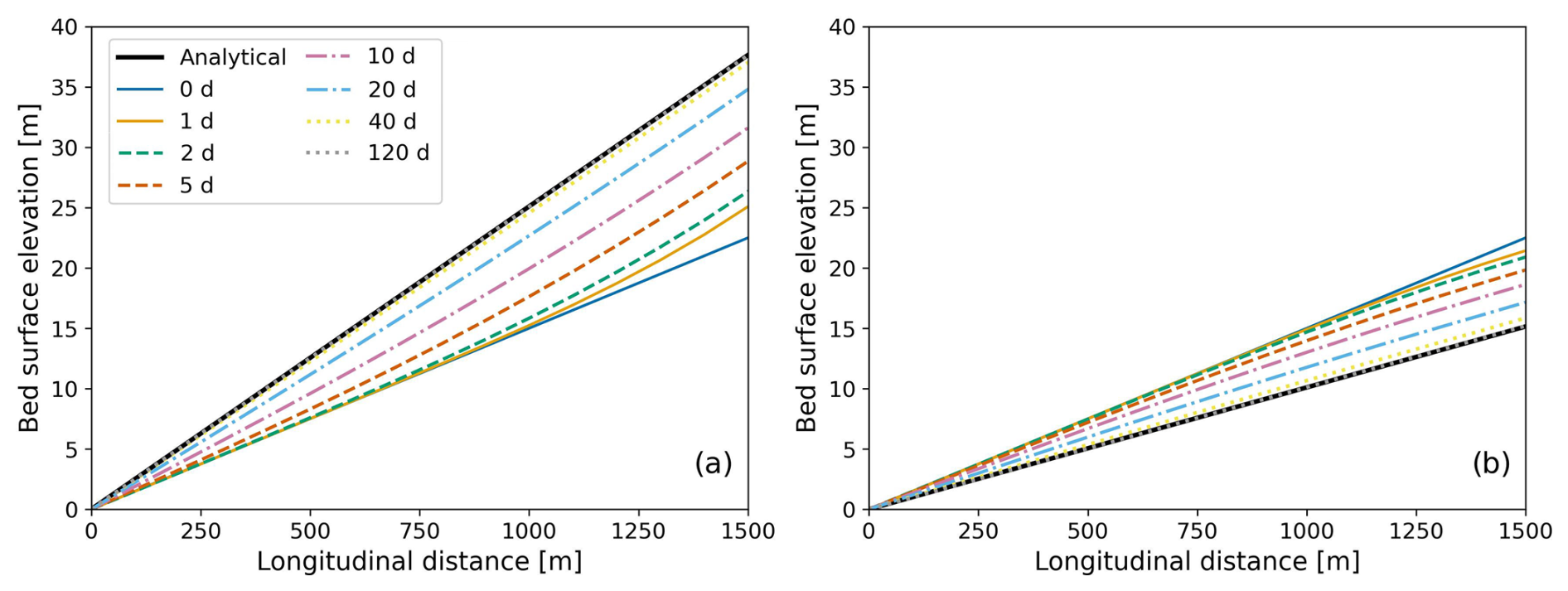
Figure 7Changes in bed surface elevation for a case of (a) pure aggradation and (b) pure degradation. The analytical solution corresponds to the equilibrium slope given by Eq. (33). The small differences in bed elevation after 40 and 120 d indicate that the systems achieved an equilibrium state.
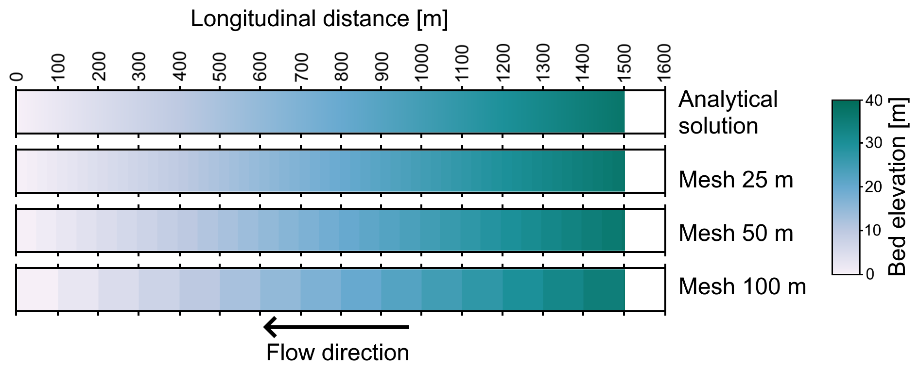
Figure 8Sensitivity of the predicted bed elevations to the grid resolution after 120 d of simulation. Three different meshes were used and compared to the analytical solution.
We analyzed the sensitivity of our results to the mesh size in the pure aggradation case by comparing the bed elevation after 120 d of simulation using meshes with half (50 m) and a quarter (25 m) of the size of the before-mentioned case (Fig. 8). By the end of each run, the average slope was 0.0251 in all cases. The percentage error in slope compared to the analytical solution was 0.29 %, 0.31 %, and 0.32 % for the 25, 50, and 100 m grid resolution, respectively. Other than the mesh size, the configuration was identical in all simulations except for the maximum time step, which was 5 s for the 100 and 50 m cases and 2.5 s for the 25 m run.
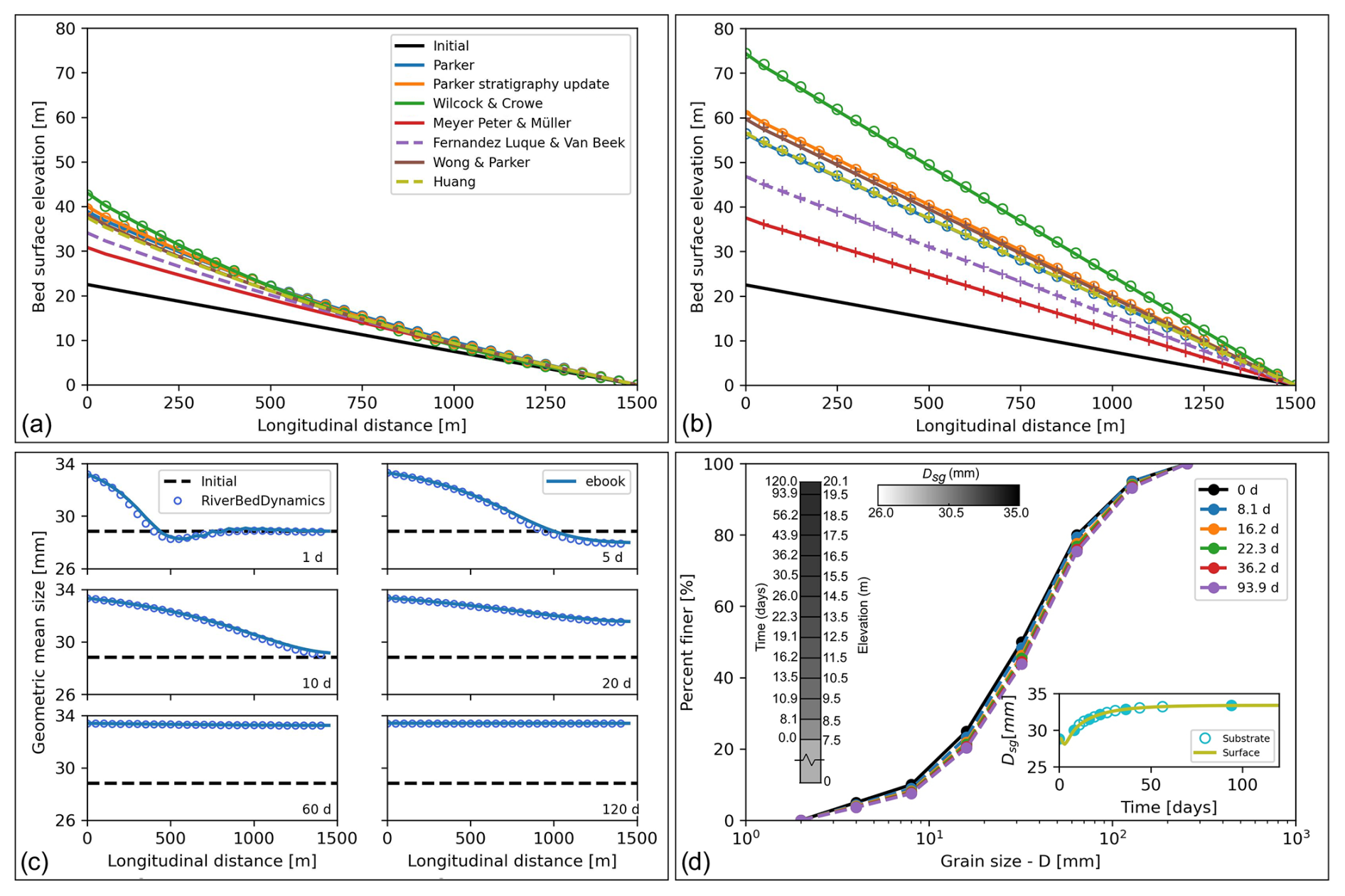
Figure 9Evolution of bed surface elevation and local grain size distribution (GSD) for all bed load transport models implemented in RiverBedDynamics. (a) Predicted longitudinal bed surface profiles after 10 d and (b) after 120 d of simulation. Continuous and dashed lines represent RiverBedDynamics results, circles indicate solutions from the e-book, and crosses denote analytical solutions. (c) Changes in space and time in the bed surface geometric mean grain size Dsg. Initial values are repeated in each panel for reference. The e-book line represents Parker's e-book solution, which is based on the Parker (1990) equations. (d) Substrate GSD evolution at x=1000 m for various simulation times. Left of the GSD curve: stratigraphic profile showing layer formation times and elevations. Top values indicate final surface elevation (20.1 m) and simulation end time (120 d). Right subplot: surface and substrate Dsg temporal changes. The substrate in this context is the layer right below the surface, as defined in Fig. 5 and Toro-Escobar et al. (1996). Circle markers denote substrate GSD update times, with filled circles corresponding to times shown in the GSD curves.
5.2 Comparing bed load transport model predictions
We checked the predictions of bed surface elevation and local GSD for all bed load transport models included in our component using a test similar to the one described in the previous section. In this case, we used a 1500 m long, straight channel with an initial bed surface slope of 0.015 m m−1, a fixed elevation of 0 m at the channel outlet, a surface roughness of n=0.0275, and a flow discharge Q=100 m3 s−1 that was generated by a rainfall intensity of 0.02 m s−1 acting over two cells of 50 m per side (Δx=Δy) located at the upstream boundary. Similar to the previous case, this configuration models a one-dimensional flow setup, utilizing a grid of uniformly sized cells with a channel width of two cells. The initial bed surface GSD had a D50 of 32 mm and Dsg of 28.84 mm, including grains ranging from 2 to 256 mm (Fig. 9d). The initial water depth (h_init) at all cells was 1 mm, and the time step was fixed and equal to 5 s. Similar to the previous test case, this time step constraint was necessary to account for the rapid bed elevation changes. Although OverlandFlow independently allows for larger time steps based on the Courant number, the coupled model demanded shorter intervals to ensure numerical stability. All other variables had their default value. The upstream sediment supply was qb=0.0075 m2 s−1 with the same GSD as the initial bed surface. The total simulation time was 120 d for all the models we ran. We choose this test configuration because our LEM predictions using the bed load equations of Parker (1990) and Wilcock and Crowe (2003) can be verified using the algorithm developed and implemented by Parker (2004), namely RTe-bookAgDegNormGravMixPW.xls (1D Sediment Transport Morphodynamics with Applications to Rivers and Turbidity Currents, http://hydrolab.illinois.edu/people/parkerg/morphodynamics_e-book.htm, last access: 1 March 2025). For the Parker (1990) equations, we considered two scenarios: one where the GSD remains constant and another where the surface and substrate GSDs are updated in line with Eq. (30). These scenarios are referred to as “Parker” and “Parker stratigraphy update” in Fig. 9. Additionally, an analytical solution for the equations of Meyer-Peter and Müller (1948), Fernandez Luque and Van Beek (1976), Wong and Parker (2006), and Huang (2010) is available using Eq. (33).
We compared the predicted channel longitudinal profiles between all bed load transport models at different simulation times (Fig. 9a and b). After 10 d, the equations of Parker (1990) and Wilcock and Crowe (2003) predicted a more concave-upward longitudinal profile and a higher elevation at the upstream boundary compared to the models that do not account for the whole GSD (Fig. 9a). The models of Meyer-Peter- and Müller-style equations had a more uniform slope along the channel profile. Comparing our LEM predictions with those from RTe-bookAgDegNormGravMixPW.xls (hereinafter, Parker's e-book), we observed good agreement in the predicted bed elevations along the channel. For Parker (1990) and Wilcock and Crowe (2003), the average errors in elevation were around 0.1 %, with a maximum local difference in bed elevation of less than 1.5 %. This corresponds to an elevation difference of 0.565 m at the upstream boundary for the Parker (1990) model that uses stratigraphy updates. There was no analytical solution after 10 d for any model because the equilibrium condition had not been reached yet.
After 120 d, all models were considered to be in relatively stable conditions, as indicated by the rate of elevation change at the upstream boundary node. The maximum elevation change was 22 mm d−1 for Wilcock and Crowe (2003), followed by 14 mm d−1 for Wong and Parker (2006) and less than 10 mm d−1 for all other models. Considering the increase of 52 m over this period at the upstream end of the model for Wilcock and Crowe (2003), the rate of 22 mm d−1 can be seen as relatively minor. Although the longitudinal profiles from all models showed a relatively uniform slope (Fig. 9b), local elevations varied. For instance, Wilcock and Crowe (2003) predicted a final bed slope of 0.0495 m m−1, almost twice as steep as the slopes predicted by Meyer-Peter and Müller (1948) at 0.0249 m m−1 and Fernandez Luque and Van Beek (1976) at 0.0311 m m−1. Parker (1990), with stratigraphy updates, predicted an average bed slope of 0.0408 m m−1.
The differences in predicted equilibrium slopes among the models reflect their distinct approaches to representing sediment transport processes. For our specific test conditions, the Meyer-Peter- and Müller-style equations (MPM, FLvB, and Wong and Parker), which predict the lowest slopes (0.0249–0.0394 m m−1), assume uniform grain size and represent transport as a simple power function of excess shear stress. In contrast, Wilcock and Crowe's model predicts steeper slopes (0.0495 m m−1) due to its distinct hiding function, which affects the relative mobility of different grain sizes. Parker's model (0.0408 m m−1) yields intermediate slopes as it uses a different hiding function formulation in its surface-based approach to grain size mixtures. While these differences highlight how the choice of transport equation can significantly impact morphological predictions, particularly in systems with diverse grain sizes, it is important to note that these results are specific to our test conditions and should not be generalized to other scenarios without careful consideration of local conditions and grain size distributions. Users should select a parameterization based on their specific application: Meyer-Peter- and Müller-style equations are suitable for uniform sediment cases, while Parker or Wilcock and Crowe's models are more appropriate for mixed-size sediments, especially when grain sorting processes are important.
Similar to the observations after 10 d, the elevation predictions of RiverBedDynamics aligned well with those in Parker's e-book and the analytical solutions. In terms of average percentage error, all predictions were below 1.4 %, with a maximum local difference in bed elevation of less than 1.1 %. This discrepancy corresponds to an elevation difference of approximately 15 cm. The elevation predicted by the Meyer-Peter- and Müller-style equations in the LEM closely matched that calculated using the equilibrium slope for the same equations (Eq. 33), with errors below 0.5 %.
Based on the results of Parker (1990) with stratigraphy updates, we analyzed the local evolution of the surface Dsg at different times during the simulation. Initially, the bed at the most upstream node quickly adjusted (Fig. 9c, 1 d panel), with Dsg increasing from 28.84 to 33.19 mm. This value remained almost constant until the end of the simulation, with a final Dsg of 33.45 mm. In the first 9 d of simulation, the bed also experienced locations of fining, indicated by local Dsg values lower than 28.84 mm. However, after 10 d and until the end of the simulation, the bed consistently had a Dsg larger than 28.84 mm across all locations. The upstream portion of the channel initially coarsened compared to the original bed grain size because the supply of upstream finer sediment was less than the transport capacity of this sized material. Such finer sediment was therefore eroded from the most upstream cells, supplying finer sediment downstream. This upstream erosion and preferential transport of the finer sediment led to the pattern of downstream fining in the beginning of the simulation (e.g., 1–10 d). However, this pattern was temporary. Given that the upstream supply of finer sediment at the simulation boundary did not replace the removed fine bed material at a sufficient rate, fine sediment was progressively winnowed throughout the entire model domain through downstream transport and vertical sorting into the subsurface. As this winnowing process continued, the initial downstream fining pattern was gradually replaced by widespread surface armoring, where coarser grains became concentrated at the surface, resulting in systematic coarsening across the domain at later time steps. This sequence illustrates the dynamic interaction between selective transport, sediment supply, and local hydraulic conditions during bed adjustment, showing how temporal changes in sediment availability can shift the dominant grain sorting pattern. On day 60, Dsg was nearly uniform throughout the domain, with 33.4 mm at x=0 and an average of 33.3 mm.
To verify the accuracy of our Dsg predictions, we compared them with those of Parker's e-book. Despite small local differences in Dsg (maximum of 1.04 mm on day 5), the magnitudes and spatial distribution matched reasonably well (Fig. 9c). The observed differences, though minor, can be attributed to the way flow is calculated. In our LEM, we used the results of OverlandFlow, a 2D flow solver that accounts for flow unsteadiness, while in Parker's e-book, the flow is predicted using simplified relations for hydraulic resistance and the normal flow (local equilibrium) approximation. It is important to note that our goal was not to replicate Parker's e-book results exactly but to have an approximate comparison to generally validate our findings.
Using this same example, we further explored the stratigraphy tracking capabilities of RiverBedDynamics, focusing on the comparison of surface and substrate GSD, particularly Dsg. For simplicity, we selected a single location at x=1000 m and analyzed it through time, thereby not investigating spatial GSD changes in this analysis. In our graphical comparison (Fig. 9d), only the topmost layer of the substrate was considered. With the default setting of bed_surf_new_layer_thick at 1 m, the first new layer was created after 8.1 d. This layer had a GSD that was, on average, coarser than the initial GSD (Fig. 9d). Throughout the 120 d simulation, a total of 12 layers were created, with the final one added after 93.9 d. Notably, 10 layers were added before 50 d, and 7 of these were added within the first 30 d. This pattern indicates that most substrate GSD updates occurred during the first quarter of the simulation, a period when bed conditions differed significantly from those observed at equilibrium (Fig. 9d subplot). The relatively minor changes in grain size distribution observed in our simulations (Fig. 9d) are consistent with the specific conditions tested, where we specified an upstream sediment supply with a grain size distribution matching the initial bed material GSD. As demonstrated by Lei et al. (2023), different sediment supply characteristics can drive more pronounced grain size sorting patterns. Future applications of RiverBedDynamics could explore such scenarios by varying both sediment supply rates and GSD, though this was beyond the scope of this model description paper.
5.3 Application to a large watershed – effect of rainfall intensity on morphological changes
Our previous bed evolution tests predominantly focused on flow in a single channel and were restricted to pure erosion or deposition. To expand on this, we conducted a final test of our LEM in a more complex and larger watershed to analyze how flow discharge and bed surface elevation vary at different locations within the domain under different rainfall events. We used a synthetic square watershed similar to that of Adams et al. (2017), covering an area of 36 km2 with a resolution of 30×30 m per cell. The watershed elevations ranged from 0 m at the basin outlet to 25 m at the highest point (Fig. 10a).
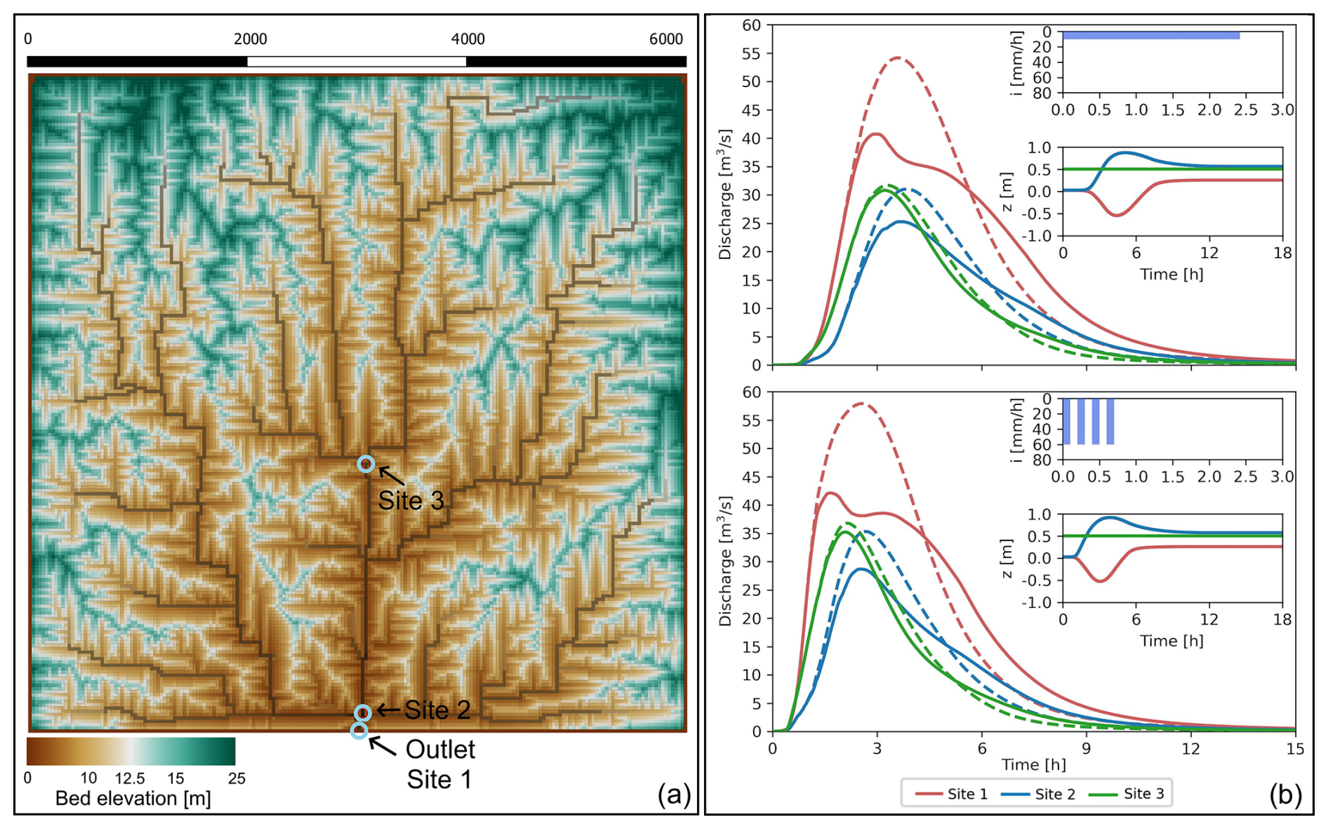
Figure 10Discharge and bed surface elevation response to different rainfall intermittency scenarios. (a) Synthetic square test basin. Three different sites, called Sites 1, 2, and 3, were chosen to represent some of the spatial variability within the watershed. (b) Hydrographs for steady- (upper panel) and intermittent-rainfall (lower panel) cases. Inset panels show hyetographs (top) and bed surface elevation (bottom) at the three sites. Dashed lines represent simulations with only OverlandFlow, while solid lines include the effects of bed elevation changes predicted by RiverBedDynamics. Rainfall intensity in the hyetographs is plotted with the vertical axis inverted to better visualize the cascading relationship between rainfall input, discharge, and bed elevation response.
For this watershed-scale application, we selected a 30×30 m grid spacing as it balances computational efficiency with the ability to capture key morphological features. While finer resolutions are possible, they become highly computationally demanding for large domains. This choice allows us to demonstrate the component's capabilities in capturing reach-scale morphodynamics while still enabling watershed-scale analysis. In a watershed of this size, grid cells are typically wider than natural channel widths, which influenced our approach to shear stress calculations. Specifically, we use water depth rather than hydraulic radius for two main reasons. First, when a cell is wider than the natural channel, most cell boundaries interface with other water-filled cells rather than channel banks, making hydraulic radius less representative of actual flow conditions. Second, our model simulates both channelized and overland flow using the same equations. Since hydraulic radius relies on the presence of defined banks, it is not applicable in overland flow conditions, further justifying the use of water depth. Although using water depth simplifies channel geometry representation, it provides reasonable estimates of reach-scale sediment transport across the watershed.
We considered two cases of temporal distributions. Both cases used spatially uniform rainfall with a total precipitation of 24 mm. We refer to these cases as (i) steady, where the rainfall intensity was 10 mm h−1, lasting for 2 h and 24 min (8640 s), and (ii) intermittent, where rainfall consisted of four cycles alternating between 60 and 0 mm h−1, with each of the two rainfall rates within a cycle lasting for 360 s (Fig. 10b). We quantified changes in flow discharge and bed surface elevation at three locations: Site 1, located at the watershed outlet; Site 2, located upstream of the outlet and at the confluence of the most downstream tributaries; and Site 3, located approximately at the center of the watershed (Fig. 10a).
We ran each model for 24 h, setting Manning's n uniformly across the watershed with a value of 0.025 and using the bed load transport equation of Meyer-Peter and Müller (1948) with a D50 of 4 mm. All other variables during the instantiation of the components had default values. We simulated each rainfall case with and without activating RiverBedDynamics (four cases in total) to analyze the effect of the selected temporal distribution of rainfall intensity on flow hydraulics (e.g., flow discharge), independent of morphodynamic changes that would also influence the hydraulics (without RiverBedDynamics), and to include the feedbacks between hydraulic and morphological changes (with RiverBedDynamics).
When running only OverlandFlow (i.e., RiverBedDynamics deactivated), the resulting hydrographs for both the steady and the intermittent cases had relatively smooth shapes at the three sites (Fig. 10b). Compared to the steady case, the intermittent scenario showed earlier and larger peak discharges at every site. For example, at Site 1 under steady conditions, the peak was 54.2 m3 s−1, arriving after 3.6 h, compared to 57.9 m3 s−1 at 2.6 h under intermittent rainfall.
With RiverBedDynamics activated, the resulting hydrograph had a lower peak discharge compared to hydrographs run using fixed bed elevations. At the outlet, for the steady-rainfall condition, the peak discharge was 40.7 m3 s−1, a reduction of almost 25 % compared to the case without bed evolution. For the intermittent case, the peak discharge was 42.1 m3 s−1, a reduction of almost 27 % compared to the case without bed evolution (Fig. 10b). At Site 2, the reductions in peak discharge for the steady and intermittent cases were about 19 % when we included effects of bed evolution. At Site 3, the changes in hydrograph shape caused by including bed evolution were relatively small, with the discharge peak decreasing by less than 5 % in both steady and intermittent scenarios.
Comparing hydrograph shapes, Sites 2 and 3 had a smooth shape, slightly skewed to the left, and with a single peak for both the steady and the intermittent cases. Site 1, at the outlet, had similar characteristics to Sites 2 and 3 for the fixed-bed-elevation case. However, when the bed elevation varied in time, the shape of the hydrograph at Site 1 changed, featuring a double peak.
RiverBedDynamics predicted alternating periods of erosion and deposition at Sites 1 and 2 for both rainfall cases. In the steady scenario, Site 1 initially eroded to −0.544 m from 0.023 m, before depositing to 0.256 m. Site 2 first deposited sediment, increasing elevation by 0.874 m, then eroded to 0.566 m. The intermittent case showed similar patterns, with Site 1 ranging between −0.526 and 0.262 m and Site 2 peaking at 0.922 m before reducing to 0.578 m. Site 3 showed negligible changes in both scenarios.
Most bed elevation changes occurred during the first 6 h of simulation, coinciding with larger discharges and shear stresses. Throughout the watershed, scour and deposition patterns were observed primarily near confluences or areas with changes in local channel direction. The total area experiencing erosion or deposition larger than 1 cm after 24 h was 5100 and 8730 m2 for the steady and intermittent scenarios, respectively.
The results presented in Sect. 4 demonstrate that RiverBedDynamics can be effectively coupled with a surface hydraulic flow solver, specifically OverlandFlow in this study, to predict the evolution of bed surface properties at a watershed scale. This initial version allows us to simulate bed changes with varying degrees of complexity. For example, when utilizing the bed load transport equation of Meyer-Peter and Müller (1948), only changes in bed elevation can be considered. However, by selecting the equations of Parker (1990) or Wilcock and Crowe (2003), we can track changes in surface and substrate bed elevations as well as GSD over time. Thus, our LEM enables users to include or exclude certain processes and details depending on their specific prediction requirements.
While our new component was developed using OverlandFlow, it can integrate with any flow solver available in Landlab due to the standardized component structure. For example, in very large watersheds, where local details are less crucial than regional changes, the KinwaveOverlandFlowModel could be used to reduce simulation time. Conversely, if small-scale information is required, the OverlandFlow version of Adams et al. (2017) may suffice. It is worth noting that some assumptions that are included in the flow solver of Adams et al. (2017), such as negligible contributions from the advection term of the shallow-water equations (Bates et al., 2010; de Almeida et al., 2012), may not be representative in a complex fluvial system. Consequently, a more comprehensive flow model may need to be developed to account for such processes. Regardless, the structure of RiverBedDynamics and other Landlab components facilitates easy model integration.
We acknowledge that our model incorporates several simplifying assumptions that could potentially impact simulation accuracy in certain scenarios. First, our solution to the Exner equation, which predicts changes in bed surface elevation, is one of the simplest formulations when working in a 2D approach (Furbish et al., 2017a). While more generalized forms of sediment mass balances have been developed and applied (e.g., Juez et al., 2016; Paola and Voller, 2005; Parker et al., 2000), we prioritized a computationally efficient implementation suitable for large-watershed applications. In our formulation, we assumed that rectangular elements could define the alignment of a channel and general flow directions on hillslopes. However, this may not be representative of channels with significant curvature. Incorporating a curvature coefficient similar to that implemented by Van De Wiel et al. (2007) could lead to more accurate results, especially near river confluences.
Second, all our test cases involved channels without macro-roughness elements, such as large boulders, vegetation, or any type of flow obstructions that can significantly alter the flow direction. While our component can theoretically be applied across a range of spatial scales (from meters to tens of meters), the computational demands of watershed-scale applications often necessitate coarser resolutions. In such cases, the effects of sub-grid-scale features like macro-roughness elements would need to be parameterized rather than explicitly represented. Future development could incorporate methods to account for these small-scale effects within coarser-resolution simulations. Although we aimed to make RiverBedDynamics as versatile as possible, we have not yet evaluated its performance when subjected to sharp local gradients in shear stress induced by obstacles.
Third, we implemented an optional slope-dependent critical shear stress equation (Mueller et al., 2005), which can be used in the models of Meyer-Peter and Müller (1948) and Fernandez Luque and Van Beek (1976). We recommend caution when using this option as it both overrides the original values and allows to vary in time as local bed slope changes, which may lead to unexpected behavior. This capability was included based on preliminary model simulations where locations with steep elevation gradients, particularly riverbanks, eroded at a faster pace than expected, resulting in artificial channel widening.
Furthermore, certain sediment transport phenomena are not included in this first release. For example, RiverBedDynamics does not account for suspended-sediment motion or its effects on bed evolution. Additionally, sharp, unnatural angles within the river bed can occur because the effects of the angle of repose (sometimes called avalanche or sediment slide models) were not included in our results (Sanchez and Wu, 2011; Song et al., 2020). Finally, we did not incorporate the effects of sediment or particle diffusion (Furbish et al., 2017b) that may smooth the bed profile, resulting in a more realistic representation (compared to having large bed angles).
RiverBedDynamics is unique among Landlab components in its ability to predict sediment deposition using a fractional grain size formulation, making it particularly suited for modeling gravel-bed rivers. Other components primarily focus on predicting bed surface elevation changes based on transport-limited or detachment-limited river assumptions. However, this advanced capability comes at a computational cost: simulations using RiverBedDynamics can take up to 1.5 times longer compared to the DetachmentLtdErosion component (even when using the simplest configuration such as MPM, no stratigraphy tracking, and constant GSD). This increased runtime may constrain the total possible simulation time. Although there are no intrinsic limitations on simulation time in RiverBedDynamics, this mechanistic approach may be better suited for modeling relatively small timescale processes.
The OverlandFlow–RiverBedDynamics approach in our LEM employs a sequential-solution strategy (Cao et al., 2002; Colombini and Stocchino, 2005). This means that the governing equations are solved separately and serially. Essentially, the flow is “paused” while the RiverBedDynamics component solves the Exner equation during a given time step (Fig. 11a and b). While the components interact through continuous feedback over multiple time steps, their equations are solved one after another within each individual step. Consequently, the selected time step must ensure relatively small bed elevation changes to maintain simulation stability. For scenarios involving flow, rainfall, and watershed conditions that generate dramatic elevation changes, an optional local correction can be used to preserve numerical stability and ensure mass conservation (Fig. 11c).
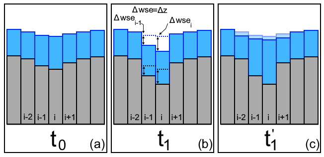
Figure 11Illustration of the local water depth correction in RiverBedDynamics, demonstrated through an erosional case (similar principles apply to deposition). (a) Initial bed and water depth condition (t0). Gray rectangles represent individual bed nodes, identified by subscript i. Light blue rectangles depict water depth. (b) Bed and water surface elevations change at nodes i−1 and i by the end of time t1, while water depth remains constant but creates unrealistic surface discontinuities. The bed erosion depth at a specific node equals the decrease in water surface elevation, and Δwsei=Δzi, where Δwse and Δz represent the change in water surface and bed elevation, respectively. Dashed black and blue lines show the change in water surface and bed elevation at t0. (c) The local correction is applied to water surface elevation for all nodes sharing a link with those that experienced elevation changes (from i−2 to i+1), smoothing the water surface profile while preserving mass conservation. Time denotes an internal cycle; simulation time does not progress during this correction. Transparent light blue areas above the water surface elevation indicate its position at time t0.
When bed elevation changes occur at a node, the initial calculation maintains the same water depth but shifts the water surface elevation by the same amount as the bed change. This can create unrealistic spatial jumps in water surface elevation between adjacent nodes that need to be smoothed while preserving discharge. The jumps occur because neighboring nodes still have their original water surface elevations. To address this, OverlandFlow runs for a few internal cycles to redistribute around the nodes experiencing bed changes and their immediate neighbors (those sharing links). During these cycles, simulation time does not advance, and the correction maintains mass conservation while achieving a smoother water surface profile. Once complete, the corrected water depths are mapped onto the grid, modifying local velocities while preserving discharge. This capability is configured in the driver file, with an example provided in the test case used in Sect. 5.4.
RiverBedDynamics represents a significant advancement in Landlab's modeling capabilities for river systems. As the first component to predict sediment deposition using a fractional grain size formulation, it is particularly suited for modeling gravel-bed rivers. Unlike other components that focus primarily on bed surface elevation changes based on transport-limited or detachment-limited assumptions, RiverBedDynamics enables more complex simulations of bed evolution. It tracks changes in both surface and substrate bed elevations as well as grain size distribution over time, allowing users to model detailed and realistic scenarios of river bed dynamics at watershed scales.
The examples included with RiverBedDynamics demonstrate its versatility, yet they represent only a subset of the diverse scenarios that can be simulated within the Landlab environment. For instance, integrating RiverBedDynamics with other components like VegCA opens up new avenues for studying vegetation competition under non-steady sediment transport regimes. This integration capability highlights the component's potential for multidisciplinary research in fluvial geomorphology and ecology. RiverBedDynamics also enables researchers to investigate the impact of changing precipitation patterns on sediment transport and channel morphology, the role of grain size sorting in determining sediment delivery to reservoirs, the effectiveness of different river restoration designs that involve gravel augmentation, and the influence of urbanization on channel stability through changes in both flow and sediment regimes. These applications demonstrate how the component's ability to simulate both erosion and deposition while tracking grain size evolution enables investigation of problems that were difficult to address with previous modeling approaches.
The model could also be used to understand how changes in climate influence bed evolution and GSD changes. Future applications could include coupling with bedrock erosion components to investigate how sediment cover and grain size distributions affect bedrock incision rates, though this would require modifications to incorporate a bedrock surface. Additionally, the component could be adapted to study sediment sorting and deposition patterns in alluvial fan environments, where changes in channel slope and width strongly influence grain size distribution and depositional processes.
While RiverBedDynamics already offers powerful modeling capabilities, there are exciting opportunities for future enhancements. One potential improvement would be implementing a time-varying Manning's roughness that responds to bed grain properties and water depth, such as the model proposed by Limerinos (1970). Additionally, future development could incorporate sub-grid parameterizations of bank erosion and channel migration processes. While our uniform grid framework cannot explicitly resolve channel widths, approaches similar to those developed by Van De Wiel et al. (2007) could inform how such processes might be represented through carefully designed parameterizations that account for grid-scale limitations. RiverBedDynamics could also benefit from adopting Landlab's unstructured grid handling system (ModelGrid). By extending the component's formulation to leverage Landlab's gridding library, the model could better represent irregular river geometries and heterogeneous topographic features in the surrounding landscape. To expand the component's applicability to longer timescales, we could implement a morphological acceleration factor (Morgan et al., 2020). This approach would allow for less frequent morphology calculations in slowly changing bed processes, extending the component's use to landscape evolution runs spanning millennia or longer while improving computational efficiency.
For applications in mountain river systems, particularly those with high-gradient longitudinal slopes, implementing the equations developed by Schneider et al. (2015) and Yager et al. (2007, 2012) could provide more accurate bed load transport calculations. This addition would enable explicit inclusion of large roughness elements and sediment-supply-limited conditions common in steep streams. Another potential refinement is the inclusion of a critical shear stress that evolves with sediment transport rate, similar to the approach of Johnson (2016). These potential enhancements build upon the strong foundation of Landlab and in particular our proposed component RiverBedDynamics, expanding their already significant capabilities in modeling complex river systems across various spatial and temporal scales.
We presented the first version of RiverBedDynamics, a Landlab component designed and built to simulate 2D sediment transport and river bed evolution with a special focus on gravel-bedded rivers. Integrating RiverBedDynamics with OverlandFlow has created an LEM capable of providing accurate and detailed predictions of bed surface evolution in terms of elevation and grain size distribution. This new LEM is physically based and solves fundamental governing equations, such as the conservation of mass in RiverBedDynamics and mass and momentum in OverlandFlow, enhancing its reliability in simulating unsteady processes. The new component is flexible enough for short- and long-term simulations depending on the number of processes that can be included in each case. Our LEM's predictions were validated against analytical and previously reported solutions, demonstrating accurate representation of changes in bed surface elevation and grain size distribution. Both purely erosional and purely depositional cases were evaluated, with processes well captured in each scenario. Additionally, we employed a synthetic watershed to illustrate how the interaction between rainfall intensity distribution and sediment transport processes influences flow discharge and bed surface evolution across the domain.
While we have designed the first version of RiverBedDynamics to be as comprehensive as possible in representing sediment transport processes, there is potential for further enhancements and generalizations to expand its capabilities. Nonetheless, our LEM has demonstrated that the combination of OverlandFlow and RiverBedDynamics offers significant potential for simulating many typical scenarios encountered in practical river management situations and fundamental scientific research. We anticipate that future developments will focus on improving the representation of bank erosion, channel migration, and the effects of the local angle of repose.
Table A1 summarizes all variables and symbols used throughout the paper, organized by their physical meaning and application within the model.
Table A1Summary of variables used in RiverBedDynamics, organized by physical categories. Each variable is presented with its symbol, definition, and units (where applicable).
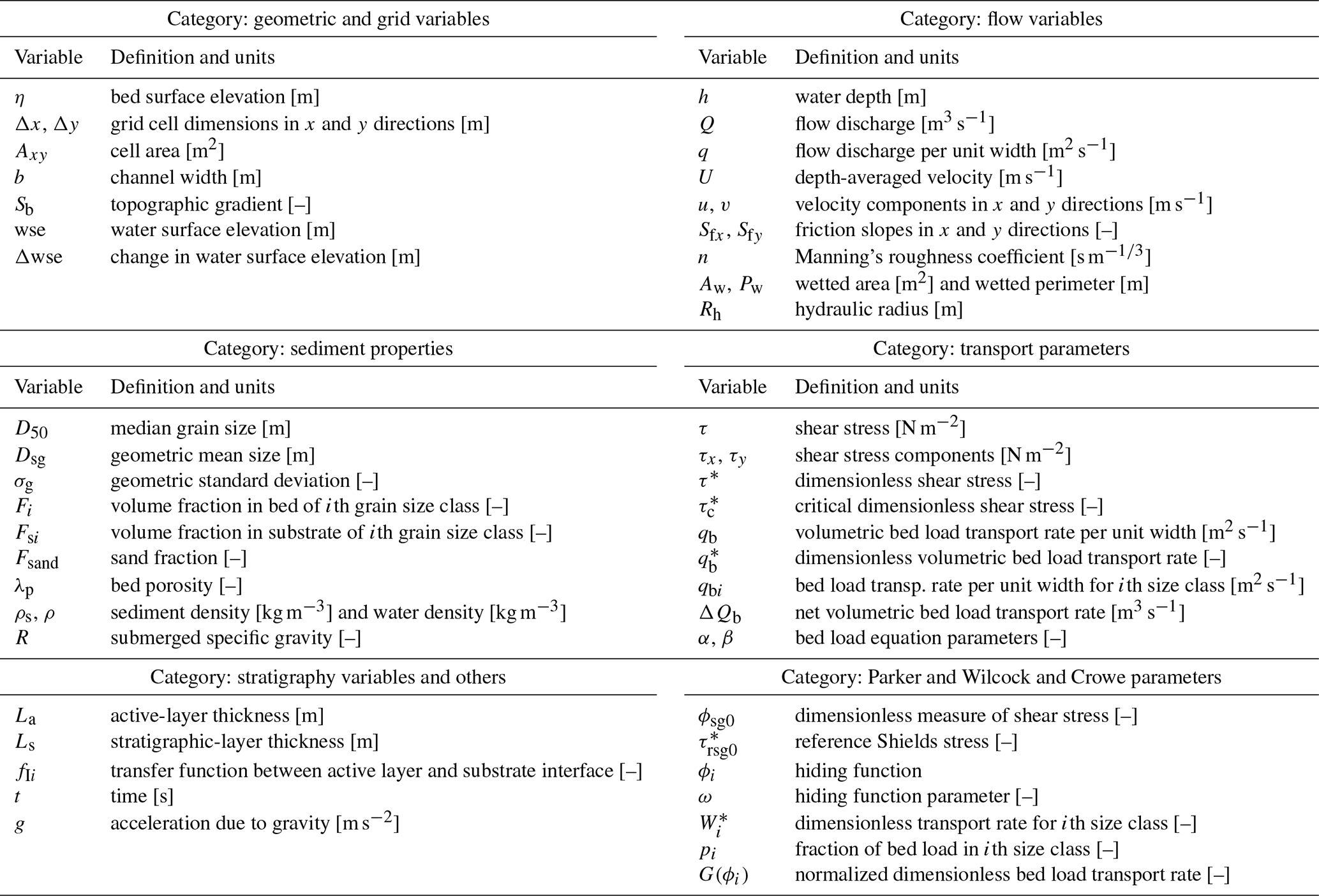
The source code for RiverBedDynamics is available in a public Zenodo repository at https://doi.org/10.5281/zenodo.14159914 (Monsalve, 2024a). This repository contains the latest release version of the component, including all necessary files for running the model within the Landlab framework.
The example scripts and data used to create and run the test cases presented in this article are accessible in a separate Zenodo repository: https://doi.org/10.5281/zenodo.14159904 (Monsalve, 2024b). This repository includes all the necessary input files, parameters, and scripts to reproduce the results discussed in this paper.
Both repositories are open source and freely available for use, modification, and distribution under the MIT License. We encourage users to refer to the README files in each repository for detailed instructions on installation, dependencies, and usage. For any questions regarding the code or data, please contact the corresponding author.
AM, SA, NG, and EY conceptualized the component and defined its requirements; AM developed the component code; SA performed alpha and beta testing; NG conducted code review and implemented improvements; AM developed the test cases with SA reviewing them; AM wrote the original manuscript draft; SA, NG, and EY reviewed and edited the paper.
The contact author has declared that none of the authors has any competing interests.
Publisher's note: Copernicus Publications remains neutral with regard to jurisdictional claims made in the text, published maps, institutional affiliations, or any other geographical representation in this paper. While Copernicus Publications makes every effort to include appropriate place names, the final responsibility lies with the authors.
This work was supported by NSF award number 1918459 to Samuel R. Anderson and Nicole M. Gasparini. We are grateful for the insightful conversations with Joel P. L. Johnson and Grace Guryan, which were instrumental in initiating this project. We extend our sincere appreciation to Eric Hutton and Mark Piper from CSDMS for their invaluable assistance during the development of this Landlab component.
This research has been supported by the NSF Directorate for Geosciences (grant no. 1918459).
This paper was edited by Boris Kaus and reviewed by Fergus McNab and one anonymous referee.
Adams, J. M., Gasparini, N. M., Hobley, D. E. J., Tucker, G. E., Hutton, E. W. H., Nudurupati, S. S., and Istanbulluoglu, E.: The Landlab v1.0 OverlandFlow component: A Python tool for computing shallow-water flow across watersheds, Geosci. Model Dev., 10, 1645–1663, https://doi.org/10.5194/gmd-10-1645-2017, 2017.
Attal, M., Cowie, P. A., Whittaker, A. C., Hobley, D., Tucker, G. E., and Roberts, G. P.: Testing fluvial erosion models using the transient response of bedrock rivers to tectonic forcing in the Apennines, Italy, J. Geophys. Res.-Earth, 116, 2010JF001875, https://doi.org/10.1029/2010JF001875, 2011.
Barnhart, K. R., Glade, R. C., Shobe, C. M., and Tucker, G. E.: Terrainbento 1.0: A Python package for multi-model analysis in long-term drainage basin evolution, Geosci. Model Dev., 12, 1267–1297, https://doi.org/10.5194/gmd-12-1267-2019, 2019.
Barnhart, K. R., Hutton, E. W. H., Tucker, G. E., Gasparini, N. M., Istanbulluoglu, E., Hobley, D. E. J., Lyons, N. J., Mouchene, M., Nudurupati, S. S., Adams, J. M., and Bandaragoda, C.: Short communication: Landlab v2.0: a software package for Earth surface dynamics, Earth Surf. Dynam., 8, 379–397, https://doi.org/10.5194/esurf-8-379-2020, 2020.
Barry, J. J., Buffington, J. M., and King, J. G.: A general power equation for predicting bed load transport rates in gravel bed rivers, Water Resour. Res., 40, 1–22, https://doi.org/10.1029/2004WR003190, 2004.
Bates, P. D., Horritt, M. S., and Fewtrell, T. J.: A simple inertial formulation of the shallow water equations for efficient two-dimensional flood inundation modelling, J. Hydrol., 387, 33–45, https://doi.org/10.1016/j.jhydrol.2010.03.027, 2010.
Braun, J. and Willett, S. D.: A very efficient O(n), implicit and parallel method to solve the stream power equation governing fluvial incision and landscape evolution, Geomorphology, 180–181, 170–179, https://doi.org/10.1016/j.geomorph.2012.10.008, 2013.
Campforts, B., Schwanghart, W., and Govers, G.: Accurate simulation of transient landscape evolution by eliminating numerical diffusion: the TTLEM 1.0 model, Earth Surf. Dynam., 5, 47–66, https://doi.org/10.5194/esurf-5-47-2017, 2017.
Cao, Z., Day, R., and Egashira, S.: Coupled and decoupled numerical modeling of flow and morphological evolution in alluvial rivers, J. Hydraul. Eng., 128, 306–321, https://doi.org/10.1061/(asce)0733-9429(2002)128:3(306), 2002.
Carretier, S., Regard, V., Abdelhafiz, Y., and Plazolles, B.: Modelling detrital cosmogenic nuclide concentrations during landscape evolution in Cidre v2.0, Geosci. Model Dev., 16, 6741–6755, https://doi.org/10.5194/gmd-16-6741-2023, 2023.
Cheng, Z., Hsu, T. J., and Calantoni, J.: SedFoam: A multi-dimensional Eulerian two-phase model for sediment transport and its application to momentary bed failure, Coast. Eng., 119, 32–50, https://doi.org/10.1016/j.coastaleng.2016.08.007, 2017.
Colombini, M. and Stocchino, A.: Coupling or decoupling bed and flow dynamics: Fast and slow sediment waves at high Froude numbers, Phys. Fluids, 17, 036602, https://doi.org/10.1063/1.1848731, 2005.
Coulthard, T. J.: Landscape evolution models: a software review, Hydrol. Process., 15, 165–173, https://doi.org/10.1002/hyp.426, 2001.
Coulthard, T. J., Macklin, M. G., and Kirkby, M. J.: A cellular model of Holocene upland river basin and alluvial fan evolution, Earth Surf. Proc. Land., 27, 269–288, https://doi.org/10.1002/esp.318, 2002.
Davy, P., Croissant, T., and Lague, D.: A precipiton method to calculate river hydrodynamics, with applications to flood prediction, landscape evolution models, and braiding instabilities, J. Geophys. Res.-Earth, 122, 1491–1512, https://doi.org/10.1002/2016JF004156, 2017.
de Almeida, G. A. M., Bates, P., Freer, J. E., and Souvignet, M.: Improving the stability of a simple formulation of the shallow water equations for 2-D flood modeling, Water Resour. Res., 48, 1–14, https://doi.org/10.1029/2011WR011570, 2012.
Fernandez Luque, R. and Van Beek, R.: Erosion And transport of bed-load sediment, J. Hydraul. Res., 14, 127–144, https://doi.org/10.1080/00221687609499677, 1976.
Forte, A. M., Yanites, B. J., and Whipple, K. X.: Complexities of landscape evolution during incision through layered stratigraphy with contrasts in rock strength, Earth Surf. Proc. Land., 41, 1736–1757, https://doi.org/10.1002/esp.3947, 2016.
Furbish, D. J., Fathel, S. L., and Schmeeckle, M. W.: Particle motions and bedload theory, in: Gravel-Bed Rivers, edited by: Tsuusumi, D. and Laronne, J. B., Wiley, 97–120, https://doi.org/10.1002/9781118971437.ch4, 2017a.
Furbish, D. J., Fathel, S. L., Schmeeckle, M. W., Jerolmack, D. J., and Schumer, R.: The elements and richness of particle diffusion during sediment transport at small timescales, Earth Surf. Proc. Land., 42, 214–237, https://doi.org/10.1002/esp.4084, 2017b.
Gasparini, N. M., Tucker, G. E., and Bras, R. L.: Network-scale dynamics of grain-size sorting: implications for downstream fining, stream-profile concavity, and drainage basin morphology, Earth Surf. Proc. Land., 29, 401–421, https://doi.org/10.1002/esp.1031, 2004.
Ghimire, B. and Deng, Z.-Q.: Event flow hydrograph-based method for shear velocity estimation, J. Hydraul. Res., 49, 272–275, https://doi.org/10.1080/00221686.2011.552463, 2011.
Goren, L., Willett, S. D., Herman, F., and Braun, J.: Coupled numerical–analytical approach to landscape evolution modeling, Earth Surf. Proc. Land., 39, 522–545, https://doi.org/10.1002/esp.3514, 2014.
Hobley, D. E. J., Adams, J. M., Siddhartha Nudurupati, S., Hutton, E. W. H., Gasparini, N. M., Istanbulluoglu, E., and Tucker, G. E.: Creative computing with Landlab: An open-source toolkit for building, coupling, and exploring two-dimensional numerical models of Earth-surface dynamics, Earth Surf. Dynam., 5, 21–46, https://doi.org/10.5194/esurf-5-21-2017, 2017.
Huang, H. Q.: Reformulation of the bed load equation of Meyer-Peter and Müller in light of the linearity theory for alluvial channel flow, Water Resour. Res., 46, 2009WR008974, https://doi.org/10.1029/2009WR008974, 2010.
Johnson, J. P. L.: Gravel threshold of motion: A state function of sediment transport disequilibrium?, Earth Surf. Dynam., 4, 685–703, https://doi.org/10.5194/esurf-4-685-2016, 2016.
Juez, C., Ferrer-Boix, C., Murillo, J., Hassan, M. A., and García-Navarro, P.: A model based on Hirano-Exner equations for two-dimensional transient flows over heterogeneous erodible beds, Adv. Water Resour., 87, 1–18, https://doi.org/10.1016/j.advwatres.2015.10.013, 2016.
Lamb, M. P., Dietrich, W. E., and Venditti, J. G.: Is the critical shields stress for incipient sediment motion dependent on channel-bed slope?, J. Geophys. Res.-Earth, 113, F02008, https://doi.org/10.1029/2007JF000831, 2008.
Langston, A. L. and Tucker, G. E.: Developing and exploring a theory for the lateral erosion of bedrock channels for use in landscape evolution models, Earth Surf. Dynam., 6, 1–27, https://doi.org/10.5194/esurf-6-1-2018, 2018.
Lei, Y., Hassan, M. A., Viparelli, E., Chartrand, S. M., An, C., Fu, X., and Hu, C.: The Effect of Sediment Supply on Pool-Riffle Morphology, Water Resour. Res., 59, e2023WR035983, https://doi.org/10.1029/2023WR035983, 2023.
Le Minor, M., Davy, P., Howarth, J., and Lague, D.: Multi Grain-Size Total Sediment Load Model Based on the Disequilibrium Length, J. Geophys. Res.-Earth, 127, e2021JF006546, https://doi.org/10.1029/2021JF006546, 2022.
Li, Q., Gasparini, N. M., and Straub, K. M.: Some signals are not the same as they appear: How do erosional landscapes transform tectonic history into sediment flux records?, Geology, 46, 407–410, https://doi.org/10.1130/G40026.1, 2018.
Limerinos, J. T.: Determination of the Manning coefficient from measured bed roughness in natural channels Roughness in Natural Channels, US Geological Survey, Washington, D.C., https://doi.org/10.3133/wsp1898B, 1970.
Mao, L., Uyttendaele, G. P., Iroumé, A., and Lenzi, M. A.: Field based analysis of sediment entrainment in two high gradient streams located in Alpine and Andine environments, Geomorphology, 93, 368–383, https://doi.org/10.1016/j.geomorph.2007.03.008, 2008.
Meyer-Peter, E. and Müller, R.: Formulas for bed-load transport, in: Proceedings of the 2nd Meeting of the International Association of Hydraulic Research, 7–9 June 1948, Stockholm, 39–64, http://resolver.tudelft.nl/uuid:4fda9b61-be28-4703-ab06-43cdc2a21bd7 (last access: 1 March 2025), 1948.
Mitchell, N. and Forte, A. M.: Tectonic advection of contacts enhances landscape transience, Earth Surf. Proc. Land., 48, 1450–1469, doi10.1002/esp.5559, 2023.
Monsalve, A.: RiverBedDynamics v1.0: A Landlab component for computing two-dimensional sediment transport and river bed evolution – Source Code (Version V1), Zenodo [code], https://doi.org/10.5281/zenodo.14159914, 2024a.
Monsalve, A.: RiverBedDynamics v1.0: A Landlab component for computing two-dimensional sediment transport and river bed evolution – Test Cases (Version V1), Zenodo [data set], https://doi.org/10.5281/zenodo.14159904, 2024b.
Morgan, J. A., Kumar, N., Horner-Devine, A. R., Ahrendt, S., Istanbullouglu, E., and Bandaragoda, C.: The use of a morphological acceleration factor in the simulation of large-scale fluvial morphodynamics, Geomorphology, 356, 107088, https://doi.org/10.1016/j.geomorph.2020.107088, 2020.
Mueller, E. R., Pitlick, J., and Nelson, J. M.: Variation in the reference Shields stress for bed load transport in gravel-bed streams and rivers, Water Resour. Res., 41, 1–10, https://doi.org/10.1029/2004WR003692, 2005.
Paola, C. and Voller, V. R.: A generalized Exner equation for sediment mass balance, J. Geophys. Res.-Earth, 110, 1–8, https://doi.org/10.1029/2004JF000274, 2005.
Parker, G.: Surface-based bedload transport relation for gravel rivers, J. Hydraul. Res., 28, 417–436, https://doi.org/10.1080/00221689009499058, 1990.
Parker, G.: Selective Sorting and abrasion of river gravel. I: Theory, J. Hydraul. Eng., 117, 131–147, 1991.
Parker, G.: 1D Sediment Transport Morphodynamics with Applications to Rivers and Turbidity Currents, http://hydrolab.illinois.edu/people/parkerg/morphodynamics_e-book.htm (last access: 1 March 2025), 2004.
Parker, G., Paola, C., and Leclair, S.: Probabilistic Exner Sediment Continuity Equation for Mixtures with no Active Layer, J. Hydraul. Eng., 126, 818–826, https://doi.org/10.1061/(ASCE)0733-9429(2000)126:11(818), 2000.
Pfeiffer, A., Barnhart, K., Czuba, J., and Hutton, E.: NetworkSedimentTransporter: A Landlab component for bed material transport through river networks, J. Open Source Softw., 5, 2341, https://doi.org/10.21105/joss.02341, 2020.
Sanchez, A. and Wu, W.: A non-equilibrium sediment transport model for coastal inlets and navigationChannels, J. Coast. Res., 2011, 39–48, https://doi.org/10.2112/SI59-005.1, 2011.
Schneider, J. M., Rickenmann, D., Turowski, J. M., Bunte, K., and Kirchner, J. W.: Applicability of bed load transport models for mixed-size sediments in steep streams considering macro-roughness, Water Resour. Res., 51, 5260–5283, https://doi.org/10.1002/2014WR016417, 2015.
Shobe, C. M., Tucker, G. E., and Barnhart, K. R.: The SPACE 1.0 model: A Landlab component for 2-D calculation of sediment transport, bedrock erosion, and landscape evolution, Geosci. Model Dev., 10, 4577–4604, https://doi.org/10.5194/gmd-10-4577-2017, 2017.
Smith, H. E. J., Monsalve, A. D., Turowski, J. M., Rickenmann, D., and Yager, E. M.: Controls of local grain size distribution, bed structure and flow conditions on sediment mobility, Earth Surf. Proc. Land., 48, 1990–2004, https://doi.org/10.1002/esp.5599, 2023.
Song, Y., Xu, Y., and Liu, X.: Physically based sand slide method in scour models based on slope-limited diffusion, J. Hydraul. Eng., 146, 1–11, https://doi.org/10.1061/(asce)hy.1943-7900.0001814, 2020.
Temme, A. J. A. M., Armitage, J., Attal, M., van Gorp, W., Coulthard, T. J., and Schoorl, J. M.: Developing, choosing and using landscape evolution models to inform field-based landscape reconstruction studies, Earth Surf. Proc. Land., 42, 2167–2183, https://doi.org/10.1002/esp.4162, 2017.
Toro-Escobar, C. M., Paola, C., and Parker, G.: Transfer function for the deposition of poorly sorted gravel in response to streambed aggradation, J. Hydraul. Res., 34, 35–53, https://doi.org/10.1080/00221689609498763, 1996.
Tucker, G. E. and Hancock, G. R.: Modelling landscape evolution, Earth Surf. Proc. Land., 35, 28–50, https://doi.org/10.1002/esp.1952, 2010.
Tucker, G. E. and Slingerland, R. L.: Erosional dynamics, flexural isostasy, and long-lived escarpments: a numerical modeling study, J. Geophys. Res., 99, 12229–12243, https://doi.org/10.1029/94jb00320, 1994.
Tucker, G. E., Lancaster, S. T., Gasparini, N. M., Bras, R. L., and Rybarczyk, S. M.: An object-oriented framework for distributed hydrologic and geomorphic modeling using triangulated irregular networks, Comput. Geosci., 27, 959–973, https://doi.org/10.1016/S0098-3004(00)00134-5, 2001.
Tucker, G. E., Hutton, E. W. H., Piper, M. D., Campforts, B., Gan, T., Barnhart, K. R., Kettner, A. J., Overeem, I., Peckham, S. D., McCready, L., and Syvitski, J.: CSDMS: A community platform for numerical modeling of Earth surface processes, Geosci. Model Dev., 15, 1413–1439, https://doi.org/10.5194/gmd-15-1413-2022, 2022.
Van De Wiel, M. J., Coulthard, T. J., Macklin, M. G., and Lewin, J.: Embedding reach-scale fluvial dynamics within the CAESAR cellular automaton landscape evolution model, Geomorphology, 90, 283–301, https://doi.org/10.1016/j.geomorph.2006.10.024, 2007.
Whipple, K. X. and Tucker, G. E.: Implications of sediment-flux-dependent river incision models for landscape evolution, J. Geophys. Res.-Solid, 107, ETG 3-1–ETG 3-20,, https://doi.org/10.1029/2000JB000044, 2002.
Whipple, K. X., Forte, A. M., DiBiase, R. A., Gasparini, N. M., and Ouimet, W. B.: Timescales of landscape response to divide migration and drainage capture: Implications for the role of divide mobility in landscape evolution, J. Geophys. Res.-Earth, 122, 248–273, https://doi.org/10.1002/2016JF003973, 2017.
Wilcock, P. R. and Crowe, J. C.: Surface-based transport model for mixed-size sediment, J. Hydraul. Eng., 129, 120–128, https://doi.org/10.1061/(ASCE)0733-9429(2003)129:2(120), 2003.
Wong, M. and Parker, G.: Reanalysis and correction of bed-load relation of Meyer-Peter and Müller using their own database, J. Hydraul. Eng., 132, 1159–1168, https://doi.org/10.1061/(ASCE)0733-9429(2006)132:11(1159), 2006.
Yager, E. M., Kirchner, J. W., and Dietrich, W. E.: Calculating bed load transport in steep boulder bed channels, Water Resour. Res., 43, W07418, https://doi.org/10.1029/2006WR005432, 2007.
Yager, E. M., Dietrich, W. E., Kirchner, J. W., and McArdell, B. W.: Prediction of sediment transport in step-pool channels, Water Resour. Res., 48, W01541, https://doi.org/10.1029/2011WR010829, 2012.
- Abstract
- Introduction
- A general overview of the Landlab modeling approach
- Model description
- Running a model using the Landlab framework
- Evaluation of RiverBedDynamics
- Discussion
- Current capabilities and future enhancements
- Conclusion
- Appendix A: Notation
- Code and data availability
- Author contributions
- Competing interests
- Disclaimer
- Acknowledgements
- Financial support
- Review statement
- References