the Creative Commons Attribution 4.0 License.
the Creative Commons Attribution 4.0 License.
 | 16 May 2025
The Multi-Compartment Hg Modeling and Analysis Project (MCHgMAP): mercury modeling to support international environmental policy
Ashu Dastoor
Hélène Angot
Johannes Bieser
Flora Brocza
Brock Edwards
Aryeh Feinberg
Xinbin Feng
Benjamin Geyman
Charikleia Gournia
Yipeng He
Ian M. Hedgecock
Ilia Ilyin
Jane Kirk
Che-Jen Lin
Igor Lehnherr
Robert Mason
David McLagan
Marilena Muntean
Peter Rafaj
Eric M. Roy
Andrei Ryjkov
Noelle E. Selin
Francesco De Simone
Anne L. Soerensen
Frits Steenhuisen
Oleg Travnikov
Shuxiao Wang
Simon Wilson
Rosa Wu
Qingru Wu
Yanxu Zhang
Wei Zhu
Scott Zolkos
The Multi-Compartment Hg (mercury) Modeling and Analysis Project (MCHgMAP) is an international multimodel research initiative intended to simulate and analyze the geospatial distributions and temporal trends of environmental Hg to inform effectiveness evaluations of two multilateral environmental agreements (MEAs): the Minamata Convention on Mercury (MC) and the Convention on Long-Range Transboundary Air Pollution (LRTAP). This MCHgMAP overview paper presents its science objectives, background, and rationale; experimental design (multimodel ensemble (MME) architecture, inputs and evaluation data, simulations, and reporting framework); and methodologies for the evaluation and analysis of simulated environmental Hg levels. The primary goals of the project are to facilitate detection and attribution of recent (observed) and future (projected) spatial patterns and temporal trends of global environmental Hg levels and identification of key knowledge gaps in Hg science and modeling to improve future effectiveness evaluation cycles of the MEAs. The current advances and challenges of Hg models, emission inventories, and observational data are examined, and an optimized multimodel experimental design is introduced to address the key policy questions of the MEAs. A common set of emissions, environmental conditions, and observation datasets is proposed (where possible) to enhance the MME comparability. A novel harmonized simulation approach between atmospheric, land, oceanic, and multimedia models is proposed to account for the short- and long-term changes in secondary Hg exchanges and to achieve mechanistic consistency of Hg levels across environmental matrices. A comprehensive set of model experiments is proposed and prioritized to ensure systematic analysis and participation of a variety of models from the scientific community.
- Article
(7218 KB) - Full-text XML
- BibTeX
- EndNote


The presence and levels of mercury (Hg) in environmental matrices of concern are associated with its primary atmospheric emissions (to air) and releases (to land and water) from anthropogenic and geogenic sources and environmental residence time. The latter is determined by physical and biochemical processes that govern the chemical and phase transformations and transport of Hg species in and across environmental matrices. Several recent studies have presented quantitative assessment of global Hg cycling (i.e., emissions and releases, concentrations, and exchange fluxes) using models and observations (e.g., Outridge et al., 2018; Zhou et al., 2021; Jiskra et al., 2021; Feinberg et al., 2022; Sonke et al. 2023). Mercury emission mitigation policies reduce Hg levels directly and by slowing the buildup of legacy Hg in soils and oceans (Angot et al., 2018; Amos et al., 2013). The effects of a changing climate (AMAP/UN Environnement, 2019; Box et al., 2019; Saros et al., 2019; Sonke et al., 2023), environmental chemical composition (e.g., Parrella et al., 2012), and land use and land cover (Zhang et al., 2016a; Feinberg et al., 2023) on Hg cycling are, however, more complex because of interactive alterations of multiple Hg processes and remobilization of legacy mercury (MacMillan et al., 2015; Yang et al., 2016; Chételat et al., 2022; Zhang et al., 2021a). Moreover, climate change impacts can vary significantly across the globe (Chételat et al., 2022; Dastoor et al., 2022a, b; Wang et al., 2020b), due to regional differences in warming. Considerations of the effects of these changes on environmental Hg cycling are warranted for assessing the effectiveness of emission mitigation policies on Hg levels. Changes in observed Hg levels exhibit combined influences of changes in multiple factors altering Hg cycling, and suitable methods are required to isolate the impacts attributable to emission policies from changes occurring due to other factors. The separate quantification of anthropogenic and natural contributions to observed changes in Hg levels is important for both understanding past changes in Hg levels and constraining projections of future Hg cycling.
The 3D single-medium or multimedia mechanistic Hg models simulate spatiotemporally resolved environmental Hg concentrations and interfacial exchange fluxes by explicitly representing intervening processes, thus allowing direct quantitative attribution of observed Hg levels and trends to emission sources and other drivers (UNEP, 2019; Zhang et al., 2016b). Furthermore, multimedia mass balance Hg models (Qureshi et al., 2011; Selin, 2014; Amos et al., 2013, 2014; Soerensen et al., 2016a) can be utilized to gain insight into the long-term fate of anthropogenic Hg emissions and releases in the biosphere reflected in the Hg records from environmental natural archives (Amos et al., 2015). To derive information from models for interpreting Hg monitoring data, reliable spatiotemporally varying anthropogenic emission inventories of Hg species from global sources are needed (Outridge et al., 2018). Equally important are the accuracy of process representations in models and observations needed for their development and evaluation. Advances in monitoring of Hg levels (atmosphere: Aas and Bohlin-Nizzetto, 2019; Sprovieri et al., 2016; terrestrial surfaces: Lim et al., 2020; Zhou et al., 2021; Wang et al., 2019; oceans: Bowman et al., 2019; Liu et al., 2020) and fluxes (air–vegetation–soil: Zhou and Obrist, 2021; Zhou et al., 2021; Gerson et al., 2022; Schneider et al., 2023; air–cryosphere: Steffen et al., 2021; freshwater–ocean: Liu et al., 2021b; Zolkos et al., 2022; air–ocean: DiMento et al., 2019; Osterwalder et al., 2021) and biochemical processes (Saiz-Lopez et al., 2020; Castro et al., 2022) continue to improve Hg models (atmosphere: Angot et al., 2016; Zhou et al., 2021; Shah et al., 2021; Feinberg et al., 2022; ocean: Rosati et al., 2022; Bieser et al., 2023; Zhang et al., 2023a). Studies have shown that application of multiple models can increase the robustness of modeling results compared to the use of single models (Travnikov et al., 2017; Bieser et al., 2017; AMAP/UN Environnement, 2019). Atmospheric multimodel ensemble (MME) simulations together with field observations, for example, led to a comprehensive assessment of contemporary Arctic Hg levels and their temporal changes, attribution, and future projections (Dastoor et al., 2022a, b; Schartup et al., 2022).
The 2013 Minamata Convention on Mercury (MC), a global multilateral environmental agreement (MEA) to protect human health and the environment from Hg pollution, requires party nations to reduce anthropogenic Hg emissions from point sources such as coal-fired power plants and certain nonferrous metal production operations and from intentional use of Hg in artisanal and small-scale gold mining (ASGM) and other industrial processes, as well as in products. The MC furthermore requires the parties to periodically evaluate its effectiveness “on the basis of available scientific, environmental, technical, financial, and economic information”, including available data on “the presence and movement of mercury and mercury compounds in the environment as well as trends in levels of mercury and mercury compounds observed in biotic media and vulnerable populations” (MC Article 22). The effectiveness evaluation (EE) is intended to address four overarching policy questions:
-
Have the parties taken actions to implement the Minamata Convention?
-
Have the actions taken resulted in changes in mercury supply, use, emissions, and releases into the environment?
-
Have those changes resulted in changes in levels of mercury in the environment, biotic media, and vulnerable populations that can be attributed to the Minamata Convention?
-
To what extent are existing measures under the Minamata Convention meeting the objective of protecting human health and the environment from mercury?
In 2021, the 4th Conference of the Parties adopted a framework for conducting the first EE (Decision MC-4/11, UNEP/MC/COP.4/28/Add.1), including creating the Open-Ended Science Group (OESG) to prepare a scientific report primarily addressing the last two overarching questions presented above. The OESG is charged with compiling and analyzing available data to address a series of guiding questions that were identified in the “Guidance on monitoring of mercury and mercury compounds to support evaluation of the effectiveness of the Minamata Convention” (UNEP/MC/COP.4/INF/12). These guiding questions address the assessment of spatial patterns, temporal trends, exposures, and adverse impacts in environmental matrices, biota, and humans and their attribution to sources and environmental processes, through the integration and analysis of observations using statistical techniques and mechanistic models. These guiding questions have been mapped to data analysis questions in the OESG's draft data analysis plan (UNEP/MC/COP.4/INF/24; https://minamataconvention.org/en/intersessional-work-and-submissions-cop-5#sec1565, last access: 1 May 2025). The OESG will provide its report to the Effectiveness Evaluation Group, who will provide findings and recommendations to the 7th Conference of the Parties (in 2027) (Decision 5/14, UNEP/MC/COP.5/25/Add.1).
The 1998 Heavy Metals Protocol of the 1979 Convention on Long-Range Transboundary Air Pollution (LRTAP), a regional MEA, commits parties to mitigating emissions of mercury (as well as cadmium and lead) from a variety of point sources and provides guidance on mitigating emissions associated with heavy metal use in manufactured products. Article 10 of the protocol requires LRTAP's Executive Body to review periodically the progress towards meeting the obligations in the protocol together with the sufficiency and effectiveness of those obligations and to evaluate whether additional emission reductions are warranted. In 2012, the Executive Body's review led to a revision of the Heavy Metals Protocol, which included more stringent emission controls and updated guidance on the best-available technologies.
Mechanistic models provide an effective framework for integrating and analyzing information across a scientific system and exploring uncertainties. In recent decades, coordinated model ensembles, such as the continuous-climate Earth system modeling initiative Coupled Model Intercomparison Project (CMIP) (Eyring et al., 2016), have become essential tools for tackling key environmental science questions regarding anthropogenic influences by facilitating multimodel experimental design, data development (drivers and observational constraints), numerical and infrastructure solutions, delivery of quantitative responses for the benefit of the research community, and national and international assessments informing policy. The MCHgMAP (Multi-Compartment Hg Modeling and Analysis Project) is a multiphase international multimodel initiative intended to consolidate a variety of Hg models in coordinated ensembles, supported by observational evaluation, to develop better understanding of past, present, and future mercury cycling and support the mercury MEAs such as the MC and LRTAP. Mercury models are susceptible to various sources of uncertainty pertaining to defining the natural state of Hg cycling, anthropogenic and environmental (physical and biochemical) forcings, process mechanisms, and their parameters and model formulations. Challenging questions remain regarding how to design and interpret mercury MME within the constraints of current scientific understanding and computational power. The overarching goal of this discussion paper is to review recent advances in mercury science (sources, processes, and models), propose a synergistic multimodel experimental design to simulate and analyze short- and long-term responses of mercury cycling to anthropogenic mercury and other forcings, and determine scientific gaps and uncertainties. A novel feature of the MCHgMAP MME design is an approach to coupling atmospheric, land, marine, and multimedia mass balance models to perform harmonized simulations of Hg cycling across environmental compartments, accounting for their changing Hg exchanges. The MCHgMAP is envisaged as a long-term initiative, each phase focusing on specific science or policy areas. The objectives of the first phase of the MCHgMAP are to analyze current spatial patterns and temporal trends of global environmental mercury to inform the first cycle of the MC EE and lay the groundwork for subsequent studies. This paper provides the required information to produce a consistent set of mercury model simulations that can presently be exploited scientifically to support the first cycle of the MC EE. Additionally, individual studies documenting the preparation of observational and emission (past and future) datasets along with assessment of their uncertainties are expected to be published, supporting the MCHgMAP initiative (GMD/ACP/BG inter-journal Special Issue, 2023).
The effectiveness evaluations of both the MC and LRTAP entail assessing the significance of anthropogenic sources influenced by the MEAs on Hg levels in the atmosphere and the receiving terrestrial and aquatic environments over time compared to other factors. Appendix A provides a detailed list of guiding questions for the MCHgMAP activities, developed to address policy questions pertaining to environmental Hg in the MC OESG data analysis plan: (1) what are the contributions of anthropogenic emissions and releases and other Hg sources to current Hg levels observed in the air, biota, humans, and other media? (2) How have these contribution levels changed over time and over the timeline of the convention? (3) How do the contribution levels and their trends vary geographically at the global scale? (4) What are the contributions of anthropogenic emissions and releases and other drivers to the temporal trends in observed Hg levels across global regions? (5) How are observed Hg levels expected to change in the future? Currently, the MCHgMAP activities do not address the MC EE objective – estimation of exposure and adverse impacts. However, the spatially distributed models, which simulate atmospheric and marine Hg concentrations and fluxes, will provide valuable data that can be used to link Hg exposure and impacts to emission sources (e.g., Giang and Selin, 2016; Zhang et al., 2021b). The objective of MME experiments is to simulate the evolution of primary and secondary sources of Hg emissions and releases in the environment: (1) to generate spatially resolved global Hg levels (concentrations and fluxes), filling monitoring gaps; (2) to detect their spatial gradients and temporal trends; (3) to attribute the levels and trends to emission sources and environmental drivers; (4) to quantify the impact of MC on Hg levels and trends; (5) to quantify uncertainty of model results; (6) to develop insights into future Hg cycling under different scenarios of implementation of the MC and other MEAs; and (7) to improve the understanding of environmental Hg processes and model representations. Since anthropogenic mercury emission inventories and observations are better defined starting around 2010, the first phase of multimodel simulations is proposed for the period 2010–2020 using harmonized mercury emissions and releases to analyze Hg temporal trends from the period beginning prior to the MC (ca. 2010) and extending as close as possible to the availability of datasets. In addition, future projections of Hg levels from 2020 to 2050 are proposed using available future Hg emission scenarios (Brocza et al., 2024).
The overview topics are organized in the following order: Hg models and their drivers (Sect. 2); sources (Sect. 3); observations (Sect. 4); MME simulation design (Sect. 5); model evaluation plan (Sect. 6); modeling analysis to inform EE (Sect. 7); modeling analysis to improve Hg science and drivers (Sect. 8); modeling of future scenarios (Sect. 9); and a summary (Sect. 10). The sections are structured to include topic relevance, a literature review, challenges, plans for the study, and current limitations and recommendations for the future.
Mercury is released to the air, land, and water in Earth's ecosystems by both geogenic and anthropogenic activities. Once released by primary sources, Hg accumulates and recirculates in environmental compartments, with wide-ranging temporal delays governed by the residence time of Hg in different reservoirs. Burial in natural archives such as deep soils, lake and marine sediments, and glacial ice ultimately immobilizes Hg from its circulation in active environments. Continuous biochemical transformations and physical processes result in Hg residence times ranging from ∼1 year in the atmosphere, surface waters, seasonal snowpacks, and sea ice and from ∼1–3 years in vegetation to 102–103 years in surface soils, subsurface waters, and glaciers. Owing to slow removal from soils and deep waters and growth in recirculation, contemporary Hg levels in the environment are well above those that can be explained by current emissions and releases. Thus, consideration of historic anthropogenic emissions and releases and their ongoing recycling in environments is important for the understanding of current and future global Hg levels and trends. Climate warming is anticipated to enhance Hg recycling due to higher surface temperatures, intensified wildfires, permafrost thaw, glacier and sea ice melt, and increased river discharge.
Re-emission of deposited Hg from planetary surfaces is often referred to as “legacy emissions” in the literature. In this paper, we refer to the recycling of deposited Hg to air from both contemporary and historic primary emissions as “secondary emissions” or “re-emissions” and reserve the term legacy emissions for representing the component of re-emissions that originate from historic primary emissions that occurred at least 1 year ago. For the effectiveness evaluation of the MEAs, it is also useful to consider legacy emissions as originating from primary emissions prior to the implementation of the MEAs.
A variety of mechanistic and empirical Hg models have been developed to trace the movement and levels of Hg in abiotic and biotic environments upon its primary emissions and releases into the atmosphere and land. These include large-scale atmospheric and oceanic models, terrestrial–hydrological models, multimedia compartmental mass balance models, and watershed-scale or site-specific food web, bioaccumulation, and risk exposure models. These models are briefly discussed below, including their drivers, applicability, and limitations.
The primary drivers of Hg cycling in surface environments are anthropogenic and geogenic emissions and releases and environmental (physical, chemical, and biological) conditions. The drivers for different types of Hg models are defined here as basic or derived quantities that induce variability or trends in Hg levels of the environmental system considered in the model. In a specific model, a given Hg driver might be treated as an external or internal forcing, depending on the model purpose and the environmental compartments and processes represented by the model.
2.1 Atmospheric models
Atmospheric models facilitate understanding of the main mechanisms governing Hg dispersion and cycling in the atmosphere (Travnikov et al., 2017). By tracing the link from emissions to deposition of Hg onto environmental surfaces, atmospheric models are used to evaluate the effectiveness of mitigation policies (e.g., Angot et al., 2018; Mulvaney et al., 2020).
Global 3D atmospheric models for Hg were developed in the late 1990s, including the GISS-CTM (Shia et al., 1999), GEOS-Chem (Selin et al., 2007), GRAHM (Dastoor and Larocque, 2004) and its later development GEM-MACH-Hg (Dastoor et al., 2021; Zhou et al., 2021), GLEMOS (Travnikov and Ilyin, 2009), ECHMERIT (Jung et al., 2009), CAM-Chem/Hg (Lei et al., 2013) and its later development CAM6-Chem/Hg v1.0 (Zhang and Zhang, 2022), and WACCM (Saiz-Lopez et al., 2022). These atmospheric models (see Table F1) are built on numerical models used to simulate climate, meteorology, and air quality.
Table F5 provides an overview of model drivers and their suggested setup for the MME. The models are driven by model-specific online or offline meteorological data. Chemical data (e.g., oxidant concentrations or photolysis rates) are needed to drive the Hg redox mechanisms and speciation (i.e., conversion between the different Hg species Hg(0), Hg(II)g, and Hg(II)p). Finally, different types of emissions are needed: (1) natural emissions (geogenic), (2) anthropogenic emissions, and (3) secondary emissions (re-emissions from land, oceans, and wildfires). Some of these drivers can be harmonized for the multimodel exercise; these are highlighted in Table F5 and described in Sect. 3.
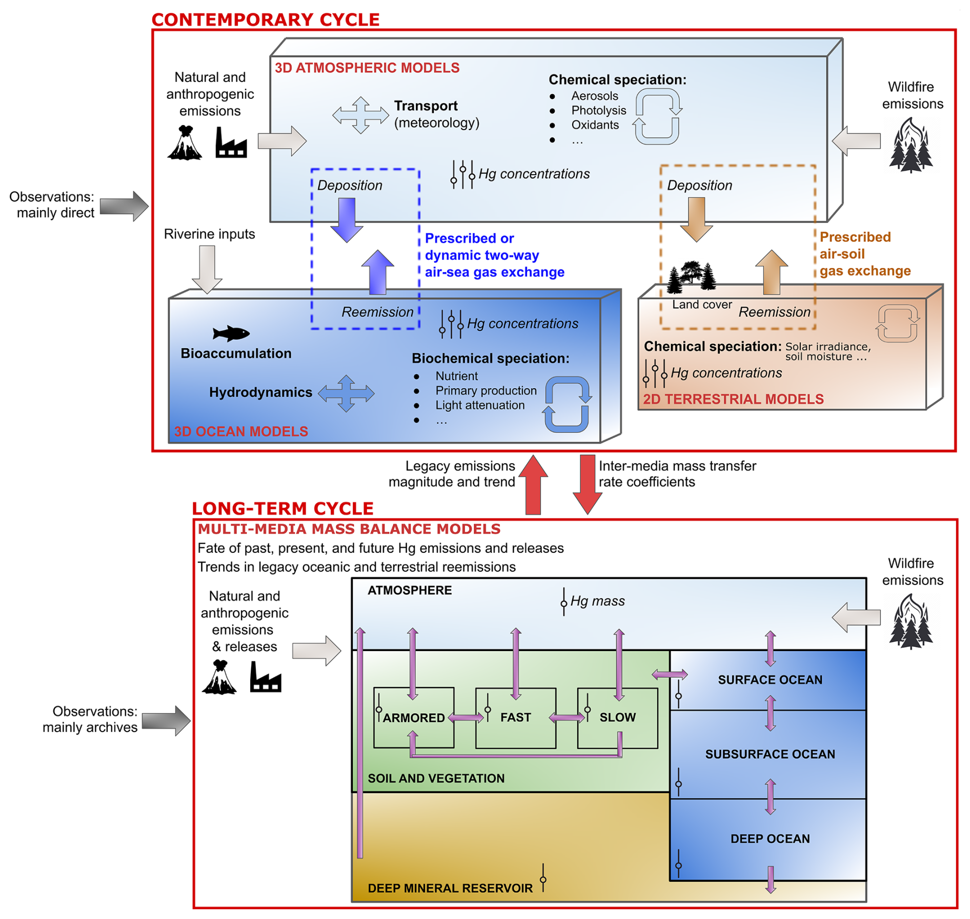
Figure 1Conceptual design of large-scale environmental Hg models and their coordination in MCHgMAP. Summary of key drivers and coupling between 3D atmospheric, 3D marine, 2D terrestrial, and multimedia mass balance models. Different configurations are possible, ranging from prescribed to dynamic two-way surface–atmosphere gas exchange.
All of the aforementioned models simulate Hg(0), Hg(II)g, and Hg(II)p concentrations (i.e., Hg speciation) along with wet and dry deposition of these species. Table F1 gives an overview of the existing global and regional 3D atmospheric Hg models and highlights the main differences in the parameterizations. The largest difference between the models relates to the parameterization of atmospheric chemistry and surface–atmosphere gas exchange. While most 3D atmospheric models use prescribed emission fluxes or formulations based on prescribed surface concentrations of Hg from the land and oceans (see Fig. 1), some models have attempted the use of a 2D surface–slab ocean and 2D terrestrial reservoir (e.g., GEOS-Chem) or even fully coupled atmospheric and ocean components (Zhang et al., 2019c). All of the models use a similar resistance-in-series dry deposition approach but with different land cover types, which may affect dry deposition fluxes. Dry deposition velocities over various surface types are estimated through the resistance analogy including aerodynamic, soil, stomatal, and cuticle resistances (Wesely, 1989; Zhang et al., 2003, 2009). Simulated Hg exchange fluxes in the canopy and underlying soils are highly sensitive to uncertain resistance parameters (Rutter et al., 2011; Zhang et al., 2019b). For example, based on micrometeorological measurements of Hg(0) fluxes, Khan et al. (2019) recommended that models increase resistances to reduce stomatal uptake of Hg(0) over grassland and tundra by factors of 5–7 and increase ground and cuticular uptake by factors of 3–4 and 2–4, respectively. Feinberg et al. (2022) later recommended a higher dry deposition velocity for Hg(0) for the rainforest land category. Terrestrial Hg(0) evasion is parameterized empirically as a function of environmental conditions (i.e., temperature, solar irradiance, or leaf area index) and legacy soil Hg content and includes a fraction of recently deposited Hg to soils, vegetation, or snow as prompt re-emission (Selin et al., 2008). Some regional models include mechanistic bidirectional atmospheric–terrestrial Hg(0) gas exchange parameterization (e.g., Bash, 2010; Wang et al., 2016c; see Sect. 3.4). The wet deposition of soluble Hg species typically includes in-cloud and below-cloud scavenging. The wet deposition flux is mostly driven by the atmospheric concentration of Hg(II) and precipitation amount (Travnikov et al., 2017). This flux is thus expected to differ among models as they use differing Hg oxidation schemes and input meteorological data. Gas exchange from the ocean surface to the atmosphere is typically parameterized based on the air–sea concentration gradient (prescribed or calculated online) and a simplified model-specific wind-speed-dependent Hg transfer velocity (see Sect. 3.5). In the absence of direct measurements of Hg(0) fluxes, this air–sea Hg gas exchange remains largely unconstrained (Zhang et al., 2019c).
Parallel to global models, regional 3D Hg models have also been developed, such as the Community Multiscale Air Quality (CMAQ-Hg) model (Bullock and Brehme, 2002), which in its latest development CMAQ-newHg-Br v2 includes a new scheme for gas–particle partitioning of mercury, replacing earlier empirical parameterizations (Wu et al., 2024) (see Table F1). They use initial and boundary conditions from global model output and allow simulations at a much finer spatial resolution (typically 1–50 km grid spacing vs. 100–300 km) over limited areas of the globe. Hg chemistry was also implemented in other regional models, including STEM-Hg (Pan et al., 2010) and WRF-Chem (Weather Research and Forecasting model coupled with Chemistry; Gencarelli et al., 2014; Ahmed et al., 2023). The global models GEOS-Chem and GEM-MACH-Hg can also be used for nested-grid simulations over specific regions (e.g., Wang et al., 2014a; Zhang et al., 2012; Fraser et al., 2018; Dai et al., 2023; Dastoor et al., 2021). A new regional model (WRF-GC-Hg v1.0; Xu et al., 2022), building on the WRF meteorological model and GEOS-Chem Hg chemistry, was recently developed using a dedicated WRF-GC coupler and allowing extra flexibility for the choice of model domain.
Despite notable improvement in modeling abilities over the past decade, several limitations and uncertainties in atmospheric Hg models can still influence our ability to evaluate source–receptor relationships and therefore limit application for policy evaluation (Kwon and Selin, 2016). Major uncertainties in atmospheric Hg modeling arise from (1) anthropogenic emissions, including emission estimates, chemical speciation, spatial distribution, and temporal changes; (2) atmospheric chemistry and phase changes, e.g., redox reactions; and (3) biogeochemical cycling, e.g., the recycling of historically deposited Hg in soils and oceans (via air–surface exchange of Hg(0)) of geogenic or anthropogenic origin in the present-day environment. As highlighted in Table F1, the chemical mechanisms and associated rate constants and air–surface Hg(0) exchange formulations used in atmospheric Hg models currently demonstrate significant variability. Sensitivity analyses and intermodel comparisons are thus required to assess uncertainties in atmospheric Hg modeling. Recent modeling assessments of Hg fluxes in global terrestrial and marine ecosystems still show high uncertainties (Zhou et al., 2021; Zhou and Obrist, 2021; Feinberg et al., 2022; Zhang et al., 2019c). Further observations and model development work in parameterizing the fundamental processes of air–surface Hg exchange are needed. The approach to assessing uncertainties in this modeling effort is discussed further in Sects. 6–9.
Distinguishing the relative contributions of historic and contemporary anthropogenic Hg emissions to atmospheric Hg concentrations (and its deposition) is important as the contemporary anthropogenic fraction informs how Hg levels are affected by mitigation policies in the short term, while the legacy fraction informs the long-term response of historically changing emissions. However, currently, most of the 3D atmospheric Hg models parameterize Hg exchange with planetary surfaces while assuming static levels of Hg in soils and oceans due to a limited understanding of processes and geospatial distributions of Hg concentrations in surface environments. Additionally, accounting for the contributions of historical changes in anthropogenic Hg emissions to recent Hg trends requires model simulations at long timescales (∼ centuries), which is computationally challenging. Thus, the current 3D atmospheric models are best suited to examine the role of changes in contemporary Hg emissions and environmental variables on the distribution of Hg levels in air and deposition.
2.2 Ocean models
Development of ocean Hg models began later than for the atmospheric Hg models, and only a limited number of models exist so far. There are several reasons for this. Firstly, ocean observations have until recently been scarce, making it difficult to evaluate models. During the last decade, global-scale oceanographic survey programs like CLIVAR and GEOTRACERS have notably increased the number of observations, but continuous measurements at fixed locations (as conducted for atmospheric Hg) are still missing. Secondly, there has been a limited mechanistic understanding of Hg chemistry in the ocean, which has made it difficult to model driving mechanisms. Thirdly, compared to the atmosphere, the ocean is a step further removed from the emission sources, as Hg entering the ocean is first transported through the atmosphere or rivers, making it more difficult to assess the effects of changing input loads.
As ocean observations and knowledge of chemistry and Hg inputs have increased in the past decades, the ocean Hg models have also become more complex (Fig. 1). In contrast to earlier treatment of oceanic Hg exchange as a boundary, most current atmospheric models now implement explicit air–sea exchange parameterization with the surface ocean. The earliest marine Hg model development was the coupling of a 2D slab ocean model, including inorganic redox chemistry and vertical transport between the air, surface ocean, and subsurface ocean, to the GEOS-Chem model (Selin et al., 2008; Strode et al., 2007; Soerensen et al., 2010). The next generation of ocean models, still limited to the inorganic Hg cycle, investigated the 3D marine Hg dynamics (Zhang et al., 2014a, 2015b; Bieser and Schrum, 2016). In addition, Soerensen et al. (2016a) developed a physical–biogeochemical multi-box ocean model that included organic Hg chemistry to estimate Hg budgets in the Baltic Sea, and Pakhomova et al. (2018) developed a 1D hydrodynamic water column model with comprehensive Hg chemistry.
In recent years, more comprehensive 3D ocean Hg models that include MeHg chemistry have been developed. Currently, four marine Hg models based on numerical 3D hydrodynamic modeling are in active use (Zhang et al., 2020, Kawai et al., 2020, Rosati et al., 2022, and Bieser et al., 2023, excluding models that are no longer actively updated). Table F2 gives an overview of published 3D ocean Hg models. While all of these models contain a complete marine Hg chemistry, including MeHg chemistry, only Zhang et al. (2021a), Rosati et al. (2022), and Bieser et al. (2023) consider uptake to and release from marine biota. This makes these three models the first hydrodynamic 3D Hg models to include the marine ecosystem. Of these, only the MITgcm (Zhang et al., 2020) and MERCY (Bieser et al., 2023) currently have the possibility of performing simulations at a global scale. Previously, Schartup et al. (2018) implemented Hg bioaccumulation in a complex marine food web model.
Table F6 provides an overview of drivers and their setup in the two primary global ocean models suggested for the MME (i.e., the MITgcm and MERCY). The ocean models are driven by external sources (river input, deposition, and air–sea exchange). These drivers will be harmonized for the model ensemble exercise. The models are driven further by physical, biological, and chemical input data, including data on the atmospheric boundary. Many marine Hg models are directly integrated into marine hydrological biogeochemical models, and thus generate their input variables internally. As they are intricately coded into a host model, typically only the physical forcing data can be harmonized. Temperature, salinity, and nutrient distribution are commonly initialized and nudged to data from the World Ocean Atlas (WOA) (Boyer et al., 2018) or run completely free after initialization. For the atmospheric forcings, reanalysis data from NCEP or ECMWF are used either directly or as forcing for a coupled meteorological model. Given this, only a limited harmonization of physical input variables can be achieved. Therefore, the physical fields need to be part of an intercomparison.
With a modular model like MERCY (Table F2), it is possible to create a setup using the exact same physical model and forcing with two different ocean Hg cycling models using the FABM interface (Bruggeman and Bolding, 2014). This allows for a quantification of the roles Hg chemistry mechanisms and partitioning play in the marine Hg cycle. Models that include Hg transfer through the food web rely on information on concentrations of individual biota species, their growth, their feeding, and their mortality rates in addition to DOC and POC concentrations from a biogeochemical ecosystem model. In these cases, only the nutrient input fields can be harmonized. As with water chemistry, it is therefore relevant to compare primary productivity and carbon content as secondary variables when evaluating results from different models.
The 3D ocean models are useful for providing mass balance estimates of Hg between the atmosphere and the global ocean, investigating the effect of Hg MEAs on the ocean and creating spatially resolved air–sea Hg exchange estimates for use in atmospheric model simulations. However, the models are still hampered by inadequate information on external sources and the uncertainty of internal chemistry and air–sea exchange parameterization. Of specific importance for simulating temporal trends are limited temporal Hg observations for model evaluation and limitations in our knowledge of temporal trends in regional and global Hg inputs from rivers, coastal erosion, and hydrothermal vents in combination with a long response time of Hg concentrations in large parts of the ocean due to the slow turnover time of water masses.
2.3 Terrestrial–hydrological models
Terrestrial–hydrological models describe Hg fluxes and transformation across the land–freshwater–marine continuum and integrate Hg cycling among atmospheric, oceanic, and terrestrial reservoirs. Such models are – relative to atmospheric and ocean Hg models (Sects. 2.1 and 2.2) – underdeveloped at global scales and are typically implemented at local to regional scales because the parameters necessarily reflect physical, hydrological, and biogeochemical processes at the catchment level (Caruso et al., 2008; Jeong et al., 2020). Early efforts include the U.S. Environmental Protection Agency IEM-2M watershed Hg cycling model, which used atmospheric Hg concentrations and deposition rates as inputs to a simple mass balance spreadsheet model that simulated Hg sinks, sources, and transformation in watershed soils and surface waters (Keating et al., 1997). Subsequent efforts developed geographic information system (GIS)-based models for improved simulation of Hg dynamics within the watershed distributary network and for assessment of relative contributions from direct and indirect atmospheric sources to Hg cycling (e.g., Ambrose et al., 2005).
Later generations of terrestrial–hydrological models probed Hg dynamics under changing future climate conditions. For instance, Golden et al. (2013) explored this in a coastal plain watershed of the mid-Atlantic United States using a multimodel ensemble approach. The three watershed models included the spatially explicit, process-based Grid-Based Mercury Model to simulate daily mass balances of water, sediment, and mercury; the Visualizing Ecosystems for Land Management Assessment Model for Mercury (VELMA-Hg), a spatially distributed mechanistic ecohydrological model that simulates surface and subsurface hydrology and nutrient and Hg dynamics; and the TOPography constituent LOADing model for mercury (TOPLOAD-Hg), an empirical load model which utilizes a physically based watershed model to simulate hydrological fluxes (of Hg) from the land to the fluvial network. While the ensemble approach helped to capture uncertainty associated with the different model conceptualizations of Hg cycling, terrestrial–hydrological models at the time were limited with respect to representation of biogeochemical processes underlying landscape Hg cycling (e.g., temperature-driven processes or availability of Hg species). Around the same time, Futter et al. (2012) published the process-based Integrated Catchments Model for Mercury (INCA-Hg), which included soil temperature and moisture, to better simulate temperature-dependent processes, and overall improved representation of Hg cycling (e.g., deposition, (de)methylation, reduction, or volatilization) in order to predict surface water Hg concentrations. Recently, Jeong et al. (2020) developed a mercury module for the Soil and Water Assessment Tool (SWAT-Hg), a GIS watershed model used to simulate climate and land use impacts on surface and groundwater hydrochemistry and contaminants, in order to address gaps in previous modeling efforts (e.g., INCA-Hg), including litterfall representation.
Development of terrestrial–hydrological Hg models over the past 25 years has made significant improvements in the representation of Hg cycling dynamics. However, from the perspective of the EE of the MEAs, the utility of these models is uniformly hindered by scaling issues. That is, no known terrestrial–hydrological model was developed for or can be readily applied at a global scale. This is, in part, because model development historically focused on addressing local to regional watershed-scale questions using GIS approaches (e.g., Ambrose et al., 2005; Jeong et al., 2020), which may be prohibitively expensive (computationally) at broader scales. Eklöf et al. (2015) developed various simple dynamic RIMs (riparian profile flow-concentration integration models) to simulate THg and MeHg in boreal streams in Sweden, demonstrating their ability to reproduce the observed variability in Hg and identify key drivers; such approaches can be utilized in upscaling terrestrial Hg models. As computing power and understanding of Hg cycling continue to improve, future generations of terrestrial–hydrological models will allow the scientific community to tackle Hg cycling questions of global relevance, like those in support of EE.
In the absence of global terrestrial–hydrological Hg models, land–atmosphere Hg exchange can be estimated using 2D terrestrial Hg models parameterizing air–terrestrial exchange. The Global Terrestrial Mercury Model (GTMM) was developed over a decade ago within the carbon cycling framework of the Carnegie–Ames–Stanford Approach (CASA) biosphere model (Smith-Downey et al., 2010), which covers the top 30 cm of the soil and consists of four soil Hg pools. However, the GTMM has not been supported recently and cannot be coupled with available atmospheric models. Recently, Yuan et al. (2023) developed a global air–land Hg model based on the Community Land Model within the Community Earth System Model (Lawrence et al., 2019) with an emphasis on Hg uptake and physiological transformations in vegetation for different plant functional types.
2.4 Multimedia mass balance models
Multimedia mass balance models describe the exchange of mercury between media, providing a relatively simple approach to bottom-up attribution of trends across spatial and temporal scales. Mass balance models typically represent mercury cycling as a set of coupled ordinary differential equations, with mercury exchange between compartments parameterized as a set of first-order rate coefficients (Qureshi et al., 2011; Amos et al., 2013, 2015). While retaining self-consistency, mass balance models provide a means of tracing the fate of anthropogenic mercury emissions and releases into the environment over decades to millennia, typically in a closed, mass-conserving system. Because of these features, mass balance models have proven themselves to be useful tools for quantifying uncertainties in the global Hg budget (Amos et al. 2014; Qureshi et al., 2011), evaluating impacts of historical anthropogenic mercury emissions (Amos et al., 2013, 2015) and projecting the consequences of future activities (Angot et al., 2018; Selin, 2014, 2018; Chen et al., 2018).
The principal challenge in constructing a mass balance model is to define an appropriate number of physically meaningful compartments for which the mercury mass and fluxes can be constrained by observations and process-based models (Fig. 1). Existing global multimedia biogeochemical cycle mass balance models (also referred to as GBC box models) typically utilize between five (Qureshi et al., 2011) and seven (Amos et al., 2013, 2015) boxes representing a single global atmospheric reservoir and one or several soil and ocean reservoirs. Significant effort has gone into compiling available budget constraints from modern observations and environmental archives (Amos et al., 2015), though uncertainties remain about the mobility and residence times of some reservoirs, including global soils and the large quantities of anthropogenic mercury released onto land and into water in forms such as mine tailings, fly ash, calomel, and consumer and industrial waste (e.g., Outridge et al., 2018; Guerrero, 2016; Streets et al., 2018, 2019a, b). A summary of the published mass balance models is provided in Table F3.
Mass balance models are typically defined by a fixed set of rates coupling mass exchange between a fixed number of compartments. These models are then forced with time-varying inputs of geogenic and anthropogenic Hg, which is mobilized from the lithosphere by processes such as volcanism, mining, and fossil fuel combustion. Trends in mass balance can be driven by (1) emission and release trends, (2) non-steady-state variation in compartment magnitude, and (3) rate variability in response to environmental change. Typically, the dependence of model rates on environmental drivers (e.g., oxidants, meteorology, and land cover) is not explicit, so time-varying rates must be specified based on extrinsic calculations. Nonetheless, time-varying rates can be easily incorporated into mass balance modeling frameworks.
Because available global mass balance models are similar in structure and composition, a fixed number of reservoirs is recommended as the basis for the MME mass balance modeling activities. Furthermore, it is proposed that a fixed set of time-invariant Hg exchange rates be compiled based on state-of-the-science estimates of contemporary reservoir masses and fluxes, as well as the associated uncertainties. These reservoir levels and rates will be used as a “base case” which can be compared to results from sensitivity analyses (see Sect. 5.3) in which emissions and rates are perturbed. The rates are calculated as , in which kij is the first-order rate coefficient describing mass transfer from reservoir i to reservoir j, based on the flux of mass from i to j (Fij) and the mass in reservoir i (mi). An example of the modern mercury budget terms used to calculate the mass balance model rates can be found in Table F7, based on the work of Amos et al. (2014). Efforts to update the budget estimates used for the base case model configuration should be based on a community effort to reach a consensus on contemporary global fluxes and reservoir magnitudes, reflecting results from both primary measurement and upscaling techniques and from process model results.
Mass balance models will be useful for estimating time-dependent global long-term trends in Hg levels in environmental reservoirs and intermedia secondary mercury emissions and releases under various primary anthropogenic emission and release scenarios. This may be important, since secondary emissions are currently the largest source of mercury in the atmosphere (Amos et al., 2013). However, because existing mass balance models are generally composed of global, time-invariant rates, they provide no information about regional differences or the effects of global change on mercury cycling. Additionally, these models typically do not explicitly represent mercury speciation. It is recommended that the GBC box model simulations be performed to generate changes in secondary mercury emissions and releases and global reservoir concentrations over longer time periods (decades–centuries); these values can in turn be used to scale boundary conditions for higher-complexity, single-medium mechanistic models such as the 3D atmospheric and marine models described above.
2.5 Emissions in exposure–risk models
The major exposure pathway for Hg is the consumption of food that is contaminated with MeHg (Zhang et al., 2021b; Selin et al., 2010). Other pathways include direct inhalation of Hg(0) vapor, such as for ASGM workers. One key step in emission–exposure–risk models is the link between the environment and food (e.g., freshwater fish, seafood, marine mammals, and rice) Hg levels. Existing studies often use matrices that are most directly associated with food Hg levels, e.g., atmospheric deposition or marine plankton MeHg concentrations for seafood, atmospheric deposition for freshwater fish, and soil concentrations for rice (Giang and Selin, 2016; Sunderland et al., 2018; Chen et al., 2019; Li et al., 2020b; Zhang et al., 2021b; Pang et al., 2022). These environmental matrices can be linked to emissions via atmospheric and oceanic Hg transport and transformation and food web and bioaccumulation models (Schartup et al., 2018). Different levels of complexity, e.g., involvement of different trophic levels or types of seafood and their geographical locations, have been considered in modeling efforts. Model parameters are generally site-specific for the food web and bioaccumulation models, which are often difficult to obtain (e.g., food web structure and water biogeochemistry) and challenging to extend to larger areas.
Exposure and human health risk assessment models represent the intake of mercury by humans and require Hg concentrations in diet items, in occupational practices (e.g., ASGM and dentistry), and in certain products (e.g., skin-lightening creams and waste products). The human health risk of the exposure to different Hg chemicals involves studies in biological and health sciences, e.g., epidemiology and pharmacokinetics, which are beyond the scope of this paper. Existing studies often consider the neurological effects of developing brains and fatal heart attacks in adults (Giang and Selin, 2016). Simple pharmacokinetics are assumed between the total MeHg exposure and human biomarker Hg levels (e.g., hair, blood, and urine Hg). The latter is then applied to quantitative dose–response relationships to obtain the health risk. Some studies also further monetize the health risk by associating it with socioeconomic parameters such as the value of a statistical life and the expected lifelong production of newborns (Zhang et al., 2021b; Pang et al., 2022).
Existing challenges include direct modeling of food Hg levels. The lack of more comprehensive and process-based rice paddy Hg and MeHg models, as well as a more comprehensive marine ecosystem model that is integrated with fishing activities, hinders accurate risk assessment. In addition, there is incomplete information about dietary intake and the lag between environment and food Hg levels, although some studies simplified this by using a pre-specified constant lagging period. A nonlinear relationship also exists for response of food to environmental Hg levels, which is especially important in diagnostic studies (e.g., Pang et al., 2022). Human biomarker data, including for hair, blood, and urine, are needed to evaluate the estimated population MeHg exposure. For example, human hair samples are especially useful and can be collected at a relatively large scale, as they are convenient, easy to measure, and representative of long-term exposure. More epidemiological studies to better quantify the health impact of Hg exposure are urgently needed, particularly for medium to low doses for cardiological diseases. The choices of risk monetization parameters are also important in policy analysis studies (e.g., Giang and Selin, 2016). Overall, we call for a comprehensive modeling approach that involves collaboration between Earth, medical, and social scientists to provide a much-needed tool to help parties evaluate MEAs.
2.6 Coordinated multimedia modeling
The primary focus of the MCHgMAP modeling plan is to simulate the mechanistic link between the primary emissions and releases of Hg (from anthropogenic and geogenic sources) and Hg levels in large-scale global abiotic environments (primarily the atmosphere and oceans) to detect and analyze their spatial patterns and temporal trends. Based on the availability and limitations of the different Hg modeling frameworks described above, application of an ensemble of 3D atmosphere, 3D ocean, 2D air–land, and multimedia mass balance models is proposed. A coordinated multimodel approach, combining the strength of multiple single-medium and multimedia mass balance Hg models, is suggested to consistently simulate Hg cycling among environmental compartments and to allow assessment of the impacts of both contemporary and historic changes in anthropogenic Hg emissions on environmental Hg levels. Current 3D mechanistic Hg models are suitable for analyzing the short-term responses of changes in both emissions and environmental conditions to spatially resolved Hg levels and trends. On the other hand, the influence of long-term changes in emissions and releases (over decades and centuries) on temporal trends of Hg levels in environmental media can be estimated by the mass balance Hg models; these estimates can in turn be used in 3D models to assess their implications for spatially distributed contemporary Hg levels and trends. Currently, the mass balance Hg models are not equipped to examine the role of changing environmental variables in Hg levels.
The conceptual construction of the proposed coordinated MCHgMAP modeling framework, including the input sources, process representations, and coupling of intermedia Hg exchange fluxes between different models, is shown in Fig. 1. The Hg sources and their proposed formulations for MCHgMAP are described in Sect. 3, followed by details of observations for model evaluation (Sect. 4). The technical details for the experimental design of the coordinated MME simulations, including the consistency of external and intermedia fluxes across the modeling framework, are described in Sect. 5.
The following sections describe the current knowledge of the spatiotemporal distributions and budgets of Hg primary emissions, re-emissions, and riverine exports, together with options for their inputs to the atmospheric, marine, and mass balance multimodel simulations proposed in this study.
3.1 Geogenic emissions
As is the case for many metal and metalloid elements, natural geogenic sources are potentially important contributors of Hg to surface environments. Volcanoes, geothermal fields, hydrothermal vents, and submarine spreading ridges release Hg from direct mantle outgassing and the remobilization of crustal deposits (Fitzgerald and Lamborg, 2014). Natural chemical and physical weathering of rocks can also release Hg from geological reservoirs, particularly within the global “mercuriferous belts” of variably Hg-enriched sediments coinciding with plate boundaries (Gustin, 2003; Rytuba, 2003).
Quantifying Hg fluxes from geogenic sources has proven difficult due to the scarcity of direct emission measurements and uncertainties associated with the relatively few data that exist (Edwards et al., 2021). Volcanic and geothermal systems in particular pose challenges for direct sampling of gas and aerosol emissions, since emission rates of Hg and other species vary over time due to changes in volcanic activity and magmatic source compositions (Pyle and Mather, 2003). While volcanic systems differ in their “emission modes”, it is widely accepted that the largest contribution of volcanic gases to surface environments is from subaerial persistently degassing volcanoes with open vents, of which there are currently ∼100 active on Earth (Carn et al., 2017; Fioletov et al., 2023). Infrequent explosive eruptions such as that in 1991 of Mt. Pinatubo may also release large “pulses” of Hg to surface environments, which are expected to perturb atmospheric and terrestrial Hg reservoirs for several years, as has been observed indirectly for large igneous province events millions of years ago (e.g., Grasby et al., 2015; Sanei et al., 2012). However, explosive eruptions are typically short-lived, contributing far less than persistently degassing volcanoes when averaged over time (Fischer et al., 2019; Fitzgerald and Lamborg, 2014; Geyman et al., 2023). Meanwhile, closed-vent degassing from dormant volcanoes and active geothermal–hydrothermal systems appears to occupy the lower end of geogenic emission sources (Fischer and Chiodini, 2015; Werner et al., 2019), although data from these sources are quite limited (Bagnato et al., 2015). The alteration and weathering of Hg-bearing rocks and soils constitute an additional component of the geogenic flux, but Hg emissions from this nonpoint source occur over large areas and pose particular challenges to quantification.
Volcanic Hg fluxes are typically estimated using Hg SO2 mass ratios calculated from coincident Hg and SO2 measurements taken within the volcanic plume. Hg is thereby indexed as an emission factor (EF) of the typically much better constrained SO2 flux from a given volcano, and the Hg flux is estimated on annual or longer timescales. However, the wide range of Hg SO2 ratios reported in the literature (spanning 10−3 to 10−7) and a lack of knowledge about these ratios' representativeness of source plume conditions contribute to the large uncertainties in most upscaled volcanic Hg fluxes. This is likely the main reason for the wide range of existing global volcanic Hg flux estimates, which span 5 orders of magnitude (0.6–7000 Mg yr−1; Bagnato et al., 2015; Ferrara et al., 2000; Geyman et al., 2023; Lamborg et al., 2006; Mason, 2009; Nriagu, 1989; Pyle and Mather, 2003; Varekamp and Buseck, 1981, 1986). By comparison, emission estimates from geothermal systems – while far fewer in number – span only 2 orders of magnitude (8.5–60 Mg yr−1 in total globally; Bagnato et al., 2015, 2018; Varekamp and Buseck, 1986). Because geothermal systems emit little to no SO2, geothermal Hg fluxes typically use CO2 as the EF; literature Hg CO2 mass ratios span –10−9 (Aiuppa et al., 2007; Bagnato et al., 2009, 2013, 2014, 2015, 2018; Engle et al., 2006; Gagliano et al., 2019; Witt et al., 2008). Due to a lack of reliable data, time-averaged contributions from infrequent explosive eruptions are more difficult to narrow down; most previous estimates are either derived from early data of questionable reliability (1000–7000 Mg yr−1; Nriagu, 1989; Varekamp and Buseck, 1986) or wrongly attributed Hg peaks in an ice core from a glacier in Wyoming (600 Mg yr−1; Chellman et al., 2017; Pyle and Mather, 2003). Given the uncertainty in this component of the volcanic Hg flux, the total geogenic Hg flux estimate may be underestimated when explosive eruptive contributions are not considered. However, the discrepancy is not expected to be great due to the larger time-averaged contributions of persistent degassing to volcanic gas release. Li et al. (2020a) recently formulated a relatively low explosive eruption flux of 20 Mg yr−1, which was only ∼11 % of their estimate of the global Hg flux from persistent degassing (179 Mg yr−1).
More recent estimates of the global volcanic flux (37–232 Mg yr−1; Bagnato et al., 2011, 2015; Fitzgerald and Lamborg, 2014; Geyman et al., 2023; Li et al., 2020a; Mason, 2009; Nriagu and Becker, 2003; Sonke et al., 2023) reflect improvements in Hg analytical methods and a more critical use of EFs to estimate Hg emissions. Importantly, they are all lower than the more variable but generally higher estimates of past decades. This narrowed range suggests that, on average, volcanic degassing contributes <5 % of total emissions to the atmosphere from primary and secondary natural sources each year (∼5000 Mg; AMAP/UN Environnement, 2019). It should be noted that virtually all available Hg flux estimate data are from subaerial (surface) volcanic systems; virtually no data exist on submarine volcanic emissions, although estimates place these figures at ≥100 Mg yr−1 (AMAP/UN Environnement, 2019; Garrett, 2000; Rubin, 1997).
3.1.1 Formulating a global geogenic Hg emission inventory
As with another potentially important natural source (wildfires; see Sect. 3.4), the most pressing issue in geogenic Hg research is a lack of data. Importantly, the existing data are spatially imbalanced; there are no Hg plume measurements from some remote volcanic areas which have elevated fluxes of other volatiles, such as Papua New Guinea (summarized in Edwards et al., 2021). Nevertheless, estimates of the geogenic source component can be formulated for the purposes of MCHgMAP simulations. In the absence of a representative catalog of direct Hg measurements, we propose estimating volcanic and geothermal point Hg sources using recent high-quality volcanic flux data for SO2 (Fioletov et al., 2023; Tournigand et al., 2020) and CO2 (Werner et al., 2019) in combination with a compilation of EFs from the literature (i.e., Hg SO2 and Hg CO2 mass ratios) published since the year 2000 using more reliable Hg analytical methods (Edwards et al., 2021; Fitzgerald et al., 1998; Li et al., 2020a, for explosive eruptions).
To estimate the contribution of geogenic emissions originating from weathered rocks, soils, and terrestrial sediments, we employ a scaling approach based on representative surface Hg flux measurements obtained from Hg-enriched zones. The spatial distribution of these emissions is determined by referencing the global mercury mineral belts (Rytuba, 2003). We will use a recent estimation of global emissions from Li et al. (2020a), which was derived from the comprehensive surface–atmosphere Hg flux database (Agnan et al., 2016; Biester and Scholz, 1997).
3.1.2 Limitations and recommendations
The major limitation of the above approach is the use of EFs to cover the large gaps in volcanic and geothermal emissions where Hg concentration data do not exist. Indeed, published volcanic EFs represent only 14 volcanoes, or ∼13 % of the total number of currently active degassing systems worldwide. This leaves many gaps in geographic coverage, where multiple factors specific to volcanic degassing may contribute to significantly higher or lower Hg fluxes than estimates derived from “one-size-fits-all” EFs.
An additional limitation of EF-based indexing approaches stems from the observation that available Hg SO2 measurements exhibit a “heavy-tailed” distribution. This implies that a small fraction of sites characterized by high Hg SO2 ratios contributes disproportionately to the cumulative global volcanic Hg flux relative to their SO2 emissions (Geyman et al., 2023). This feature of the Hg SO2 distribution can be accounted for in global estimates of volcanic Hg flux (Geyman et al., 2023), but it fails to identify where and when these higher Hg SO2 sites occur. Improvements in understanding of the underlying drivers of variation in Hg SO2 ratios could therefore improve the accuracy of both the absolute magnitudes and the spatiotemporal distribution of volcanic Hg emissions.
Moreover, temporal changes in EFs require further attention. Previous research has shown that Hg SO2 mass ratios can change over time due to decoupled degassing behavior of the different gas species (Aiuppa et al., 2007; Siegel and Siegel, 1984), although recent work has demonstrated that Hg SO2 remains conservative over at least several hundred meters from the volcanic source (Edwards et al., 2024). As the quality and temporal resolution of SO2 and CO2 flux data increasingly improve, plume Hg measurements of “unmeasured” volcanoes are greatly needed to better understand the range of EFs and the representativeness of the single EF used for the respective geogenic Hg flux calculations of persistent degassing volcanoes, geothermal systems, and infrequent explosive eruptions. Measurements of eruption plume Hg using modern-day analytical techniques and aerial sampling platforms (e.g., drones) should be a priority for future volcanic Hg work.
One additional limitation concerns the speciation of volcanic Hg upon emission and downwind of the source, which has important implications for the atmospheric lifetime and environmental fate of Hg within the broader Hg cycle. While GEM appears to be the dominant Hg species in near-source volcanic plumes > 95 % (Bagnato et al., 2007; Martin et al., 2011; Witt et al., 2008), some measurements of aged volcanic plumes show gaseous oxidized Hg (Hg(II)g) and particulate-bound Hg (Hg(II)p) concentrations well above background levels (Aiuppa et al., 2004; Ravindra Babu et al., 2022; Dedeurwaerder et al., 1982; Galindo et al., 1998). Further work focusing on the downwind physicochemical fate of Hg after emission is therefore essential for grasping the environmental significance of geogenic emissions within the larger Hg cycle.
3.2 Anthropogenic emissions
Global anthropogenic Hg activities accounted for ∼30 % of the total Hg emissions to the atmosphere in 2015 (Outridge et al., 2018). Anthropogenic Hg emissions can be from intentional Hg use activities, the production and use of Hg-added products, and the unintentional Hg emission sectors where Hg is an impurity in the raw materials or fuels. The history of atmospheric Hg emissions can be traced back over 4000 years (Bebout, 2006). However, currently available emission estimates only represent emissions during the last 500 years (Streets et al., 2019a), and comprehensive global inventories only represent the most recent 50 years (AMAP/UN Environnement, 2019; Wu et al., 2016; Liu et al., 2019a; Muntean et al., 2014, 2018; Zhang et al., 2016b; Pacyna et al., 2006a, 2010; Pacyna and Pacyna, 2002). Anthropogenic Hg emissions vary temporally and spatially and depend on the effects of economic, policy, and human activities in different regions. Understanding the sectoral, temporal, spatial, and chemical speciation variations of current Hg emissions is essential for simulating the global transport and deposition of atmospheric Hg and evaluating ecological and human benefits from Hg pollution control policies. In addition, Hg can take millennia to be returned to a secure and long-term (environmental) repository. Determining where and when Hg is released as a result of human activities allows better quantification of present-day secondary emissions and releases and future trajectories of environmental concentrations.
Mercury governance under the MEAs
The mercury MEAs (MC and LRTAP) set out to protect human health and the environment by mitigating anthropogenic Hg emissions and releases. The Minamata Convention includes provisions for eliminating Hg mining and introduces trade-related provisions and targets to phase out or reduce Hg uses in consumer products, industrial processes, and ASGM. Such actions will benefit Hg emission reduction from intentional Hg use sectors. In addition, the convention sets out emission control obligations for five source categories responsible for the largest proportion of point source atmospheric Hg emissions: coal-fired power plants, coal-fired industrial boilers, nonferrous metal smelting (zinc, lead, copper, and large-scale gold production), waste incineration, and cement clinker production. To formulate emission control policies and evaluate the convention's effectiveness, each party shall establish, as soon as practicable and no later than 5 years after the date of entry into force of the convention, and maintain thereafter, an inventory of emissions from relevant sources (MC Article 8, Paragraph 7). However, it should be noted that parties are only required to maintain information on emissions from the five convention-related point source categories and are only required to identify sources that comprise at least 75 % of the estimated emissions from each of those categories (MC Article 8, Para 2(b)). LRTAP requires parties to maintain and submit an annual inventory for anthropogenic Hg sources, but these are also often limited to specific sources covered by the agreement (ECE/EB.AIR/115; https://unece.org/sites/default/files/2021-10/ECE.EB_.AIR_.115_ENG.pdf, last access: 1 May 2025).
Therefore, emission datasets from other sources are essential for having a comprehensive estimate of anthropogenic emissions for the purposes of simulating Hg levels in the environment. In the following section, we review currently available emission data and identify plans for compiling model-ready emission inventories that can be used in MCHgMAP MME simulations.
3.2.1 Historical emissions
Overview of global and regional emission inventories
Currently, there are four main datasets of global anthropogenic emission inventories, identified here as the Arctic Monitoring and Assessment Programme/UNEP Global Mercury Assessment (AMAP/GMA; Steenhuisen and Wilson, 2019), the Emissions Database for Global Atmospheric Research (EDGAR; Muntean et al., 2018), STREETS (Streets et al., 2019b), and WHET (Zhang et al., 2016b). Table E1 summarizes the available global and regional anthropogenic emission inventories, including their methodologies, years of emission inventories, chemical speciation, and uncertainties. Previously, the 1990, 1995, 2000, and 2005 AMAP emission datasets were compiled by using sector-specific emission factors and sectoral activity data by nation (Pacyna and Pacyna, 2002; AMAP/UNEP, 2008). The improved methodology employed to produce the AMAP/GMA 2010 and 2015 emission datasets adapted this approach to also include multiple fuel- or raw-material-specific emission factors for a given sector as well as emission control technology factors derived from emission estimates that consider activity data, the associated Hg content of fuels and raw materials, the types of processes involved, and the technology applied to reduce emissions to the air (through technology profiles that reflect the degree of application and the degree of effectiveness of air pollution control) (AMAP/UNEP, 2013; AMAP/UN Environnement, 2019). We refer to the emission methodology that traces mass conservation of Hg through the process (such as those used for AMAP/GMA 2010 and 2015 emissions) as the “mass flow approach” in the remainder of this paper. Thus, the AMAP 1990–2005 and AMAP/GMA 2010–2015 inventories would not be consistent with each other. The EDGAR datasets were compiled using the mass flow approach, similar to AMAP/GMA 2010–2015 (Muntean et al., 2014, 2018). A trend of global anthropogenic emission of mercury into the atmosphere from 1510 to 2010 was developed by Streets et al. (2019a), which is the available emission inventory at the longest timescale. Subsequently, Streets et al. (2019b) developed an emission inventory covering the years 2010–2015, with slight adjustment of the emission sectors. Some of the sectoral activity data were only available at the regional (multi-country) scale. Default settings in the WHET dataset (Zhang et al., 2016b) mainly originated from Streets et al. (2011), but key national emissions such as the emissions in China (Zhang et al., 2015a) were updated according to regional inventories.
The mass flow approaches are also used in national or regional emission inventories, such as Abacas-EI-Hg in China (Wu et al., 2016) and the emission inventories for Thailand and South Korea (Wongsoonthornchai et al., 2016; Sung et al., 2018). These national studies adopted local parameters and provided the possibility of compiling more refined emission maps than the global inventories. For example, more than 90% of mercury emissions in Abacas-EI-Hg are from point sources. Some national emission inventories adopted the default sector-specific emission factors provided by the UNEP toolkit (Pudasainee et al., 2014) or estimated from local field tests, especially in the Minamata Initial Assessment (MIA) reports (Back et al., 2019). To date, the number of countries submitting MIA reports has reached 70. Facility reporting is also a commonly used method for compiling national emission inventories. Currently, approximately 44 countries have adopted the Pollutant Release and Transfer Register (PRTR) system; most of these are for countries located in Europe (https://environment.ec.europa.eu/topics/industrial-emissions-and-safety/european-pollutant-release-and-transfer-register-e-prtr_en, last access: 1 May 2025). These PRTR systems provide the basic facility data to compile a national emission inventory; however, they may only include facilities with emissions above a specified threshold.
Sectors responsible for the majority of atmospheric Hg emissions are largely accounted for in most global inventories. However, source categories in these inventories are not identical; not only do the sectors included differ, but the way in which the sectors are defined also differ. For example, in some inventories cement emissions may appear under a general category of stationary combustion that could include power plant or other industrial sector emissions. Even in the emissions compiled by one group, the source categories can change in the inventories of different years for many reasons, such as new understanding of emission sources or more available data. Compared to AMAP datasets before 2005, additional sectors such as artisanal and small-scale gold mining and waste from mercury-containing products were added in AMAP/GMA inventories for 2010 and 2015 (AMAP/UNEP, 2013; AMAP/UN Environnement, 2019). International shipping is included as a new Hg emission source in the EDGAR datasets, with a contribution of less than 1 % (Muntean et al., 2014, 2018). Cremation is only discussed in the AMAP/GMA inventory and had a low contribution. The assessed years of these inventories also varied.
Uncertainty range is an important index for reflecting the accuracy of estimated emissions. The reported uncertainties of the estimated total global anthropogenic Hg emissions are −10 % to +27 % for the AMAP/GMA dataset for 2015 (AMAP/UN Environnement, 2019), −26 % to +33 % for the EDGAR dataset for 2012 (Muntean et al., 2018), −20 % to +44 % for the STREETS dataset for 2015 (Streets et al., 2019b), and −33 % to +60 % for the WHET dataset for 2010 (Zhang et al., 2016b). However, different methods are used to quantify uncertainties, and any direct comparison of these uncertainty ranges could result in misleading conclusions; the subjectivity of assigning errors to the parameters themselves also affects the uncertainty ranges of the final emission estimates. A semi-quantitative approach to grading all the parameters in Hg emission factors is one of the most common methods used to evaluate the uncertainty of emissions. Such methods are simple, are arguably only applicable to the deterministic emission factor model, and have relatively higher reliability. The AMAP/GMA 2015 work applied a “propagation of errors” approach to quantify uncertainty, similar to the approach applied in some IPCC work. Quantitative approaches based on Monte Carlo simulations to produce probabilistic emission estimates by taking into account the probability distribution of key parameters have been widely used in emission inventories in the past decade. Such methods are believed to be more objective, but a more sophisticated scheme usually needs more data and more assumptions to support its application.
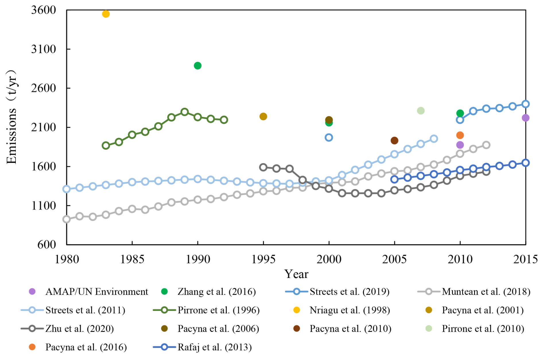
Figure 2Temporal trends of global anthropogenic Hg emissions to the air based on the available inventories (AMAP/UN Environnement, 2019; Streets et al., 2011; Zhu et al., 2020; Pacyna et al., 2001, 2006a, 2010, 2016; Zhang et al., 2016b; Rafaj et al., 2013; Streets et al., 2019b; Muntean et al., 2018; Pirrone et al., 1996, 1998, 2010).
Historical trends and sectoral contributions
EDGAR datasets reported anthropogenic Hg emissions for the period 1970–2012, with the emissions increasing from 860 to 1889 Mg yr−1 during this period (Fig. 2). According to the STREETS datasets, emissions grew from 1971 to 2390 Mg yr−1 during 2000–2015. AMAP/GMA indicated atmospheric Hg emissions of 1810 Mg yr−1 in 2010 and 2220 Mg yr−1 in 2015. WHET assessed Hg emissions at 2890, 2160, and 2280 Mg yr−1 in 1990, 2000, and 2010, respectively. It is obvious that both the emission trends and emission amounts in typical years from current studies are not comparable. Global annual anthropogenic emissions in 1990 reached as high as approximately 2890 Mg yr−1 in the WHET dataset, while the emissions were only half of this in the EDGAR datasets. According to the WHET datasets, global emissions were suggested to decrease during 1990–2000, whereas the converse trend was suggested in the EDGAR datasets. As for sectoral emission trends after 2000, both the STREETS and EDGAR datasets indicated an upward emission trend in the industrial and fossil fuel combustion sectors.
The differences in the estimates of the total Hg emissions between different inventories before 2010 are particularly significant. Some explanations for these differences can be hypothesized. However, the reasons for the apparent differences need to be understood better. Different source classification criteria (Table E2) are certainly a part of the explanation for the differences between different inventories. For example, STREETS 2015 estimated Hg from pesticides and fertilizer, which was not included in AMAP/GMA 2015. Conversely, the AMAP/GMA 2015 inventory included Hg emissions from biomass burning, cremation, and gas combustion, which reached 56.3 Mg yr−1 in total. Emissions from waste streams of mercury-added products were included in the AMAP/GMA 2010 and 2015 inventories but not in earlier AMAP inventories (1990–2005). Even for one emission data source, the source coverage may therefore vary over time.
In Fig. 3, we present the emissions of dominant sources, mainly the MC-related sectors associated with five large point sources in Annex D of Article 8, from different inventories. In 2010, the differences between emission estimates from the coal-fired sector and from cement production were within 12 %. However, emissions from nonferrous metal smelting and waste incineration were subject to much larger differences. Hg emissions from nonferrous metal smelting in EDGAR were approximately 50 % lower than the estimation by AMAP/GMA and STREETS. It should be noted that the specific types of nonferrous metals studied were not identical, although their emission estimates were similar between AMAP/GMA and STREETS. In AMAP/GMA, emissions from aluminum smelting were included when not in the STREETS datasets. Emission differences from waste incineration between different studies were even larger. The emissions from STREETS were approximately 8 times that from EDGAR and 3 times that from AMAP/GMA. Such differences were mainly due to the inclusion of emissions caused by disposing of wastes from commercial Hg use sectors in the STREETS dataset. In AMAP/GMA 2015, emissions from the disposal of Hg-added products were also included. However, the estimated Hg emissions from waste disposal were still only half those of the STREETS dataset. Therefore, atmospheric mercury emissions from the waste incineration sector still have high uncertainty, which can be attributed to a large variation of the mercury content in the wastes, various waste types, and waste disposal methods.
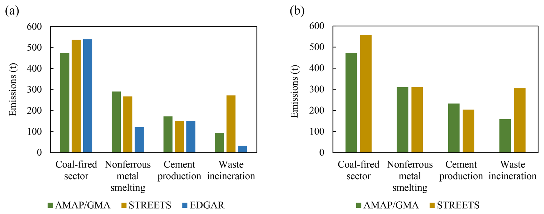
Figure 3Hg emissions of dominant sources from different inventories in (a) 2010 and (b) 2015.
Nonferrous metal smelting included zinc, lead, copper, aluminum, and large-scale gold production in AMAP/GMA and EDGAR, whereas aluminum was excluded in STREETS.
Spatial distribution
Methodologies used to produce spatially distributed emission datasets have evolved over the last 2 decades. Earlier work distributed all anthropogenic emissions on a 1°×1° or 0.5°×0.5° latitude–longitude grid using a population distribution (population density) proxy. Recent datasets, which produce a more refined resolution, incorporate more information on point source emissions (e.g., Steenhuisen and Wilson, 2019) and use different proxy data to estimate the spatial distribution for different source sectors (see Table E3). The spatial resolution of the STREETS 2010 and WHET 2010 inventories is 1°×1°, whereas EDGAR provided emissions with a resolution of 0.1°×0.1°. The spatial resolution of the AMAP/GMA 2015 dataset in UNEP (2019) was 0.25°×0.25° as its default (but a 0.1°×0.1° resolution is also available) (Steenhuisen and Wilson, 2019). However, high spatial resolution is only more accurate when point source coordinates or the proxy data themselves are available at high resolution. In general, a proxy data resolution tends to be much lower than would justify higher precision of spatial distributions.
Table E3 shows the proxy rasters applied to the various sectors in the geospatial distribution of emissions. Generally, there is a desire to obtain facility-level emission data based on the point source activity level and air pollution control information, especially for fuel combustion and industrial sources associated with large point sources. However, such data are seldom available except for a very few large point source facilities. Improvements in facility information, and in some cases emission quantification at the facility level, are a feature of both global and regional emission inventories. Emission inventories compiled based on point source information are supposed to be subject to lower emission uncertainty and higher spatial distribution accuracy. This is true when available point source coordinates and emissions or proxy data are at high resolution. However, a more sophisticated scheme usually needs more work, especially to compile a global emission inventory and maintain up-to-date facility-level information.
Therefore, point source information and spatial proxies are used to distribute emissions that are by their nature associated with diffuse sources or where the location and relevant characterization of point sources are unknown. The distribution intensity of the proxy is assumed to be a reasonable surrogate for the intensity of emissions within the studied geographical extent. Different proxies were applied to emissions from different sectors based on the available data. In the AMAP/GMA work, for example, for the stationary combustion sector or industrial sector, an industrial activity mask derived from an inventory of carbon emission point sources produced by the Carbon Monitoring for Action (CARMA) organization, facility capacity, or revenue based on industrial enterprises was generally used as a surrogate. Population remains a commonly used proxy for geospatial distribution of emissions from sectors such as waste disposal, residential heating, and some intentional uses of mercury, which are essentially diffused sources by nature.
Due to the application of different proxy rasters, the spatial distribution of emissions varies by inventory. Here, the gridded emissions are normalized to compare the emission distribution differences in different inventories (Fig. 4). A relatively large proportion of Hg was distributed in South Africa and Southeast Asia in STREETS 2010. In addition, the emission in the STREETS 2010 dataset is more scattered, whereas more high-emission grids can be observed in EDGAR 2010 and AMAP 2010. Such a phenomenon is especially obvious in East and South Asia, Europe, and North America. Moreover, Hg emissions calculated for international shipping by multiplying the fuel consumption by emission factors led to emissions on the ocean surface in the EDGAR 2010 dataset that are absent in STREETS 2010 and AMAP/GMA 2010.
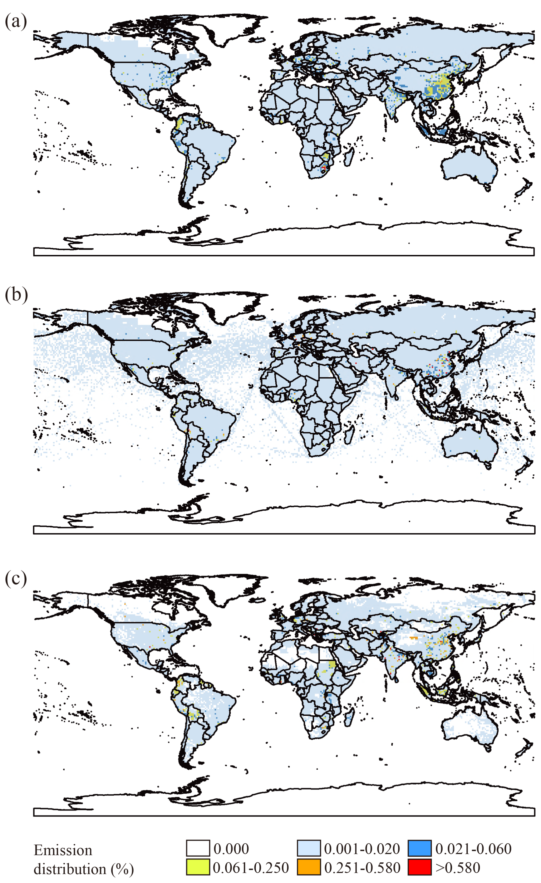
Figure 4Spatial distribution of anthropogenic Hg emissions in different inventories: the (a) STREETS dataset 2010 (Streets et al., 2019b), (b) EDGAR dataset 2010 (Muntean et al., 2018), and (c) AMAP/GMA dataset (AMAP/UNEP, 2013).
Chemical speciation
Together with the spatial distribution, characterization of the emitted forms of Hg has been identified as a major challenge and recognized in the AMAP/GMA work as an area requiring attention in the future. Both subjects are of importance for Hg transport and fate modeling. In several of the global inventories, the emissions of different forms of Hg (Hg(0), Hg(II)g, and Hg(II)p) have been derived by multiplying the total Hg emissions by “Hg speciation profiles” (i.e., percentages of the mercury in each of the three forms emitted). Hg speciation profiles can differ between sectors due to differences in fuel consumption and fuel type, control devices for air pollutants, and operating procedures. Table E4 compares the speciation profiles (%) used in the AMAP/GMA, WHET, and EDGAR inventories. AMAP/GMA and WHET used sector-specific speciation profiles. Many recent publications have reported results of measurements of Hg species under various plant-operating conditions and for different applied technologies, including air pollution control technologies. These studies provide the possibility of applying technology-specific speciation profiles, such as that used in the EDGAR datasets. The functionality of the spatial distribution application employed in AMAP/GMA to generate a speciated global inventory has been developed to make it more flexible, e.g., with respect to applying more complex speciation schemes based on country technology levels. As part of the AMAP/GMA work, Steenhuisen and Wilson (2019) investigated the effect of applying different speciation schemes for emissions from China, utilizing the information presented in Zhang et al. (2015a) for all sectors other than ASGM. However, it was not considered justified to adapt this scheme to the entire global inventory, as this would imply that all countries apply a similar (and, in the case of newly constructed large point sources, relatively advanced) control technology to China. The limitations of continuing to use the older default speciation scheme for much of the AMAP/GMA 2015 inventory work was however fully acknowledged.
Due to the differences in speciation profiles, sectoral emission contributions, and spatial proxies in different studies, the proportion of the three Hg forms in the same grid cell varied by inventory, as shown in Fig. 5. Overall, the emission share of Hg(0) from AMAP/GMA 2010 was generally higher than those from STREETS 2010 and EDGAR 2010. In all three of these datasets, there were cells with a Hg(0) proportion higher than 80 % in central Africa and South America, whereas an overall Hg(0) emission proportion higher than 80 % in North America is only found in STREETS 2010. The Hg(II)g proportion in the EDGAR datasets was mainly located in the range 20 %–60 %, which is much higher than the proportion in the other two datasets. The emission proportion of Hg(II)p in all three inventories was lower than 20 %.
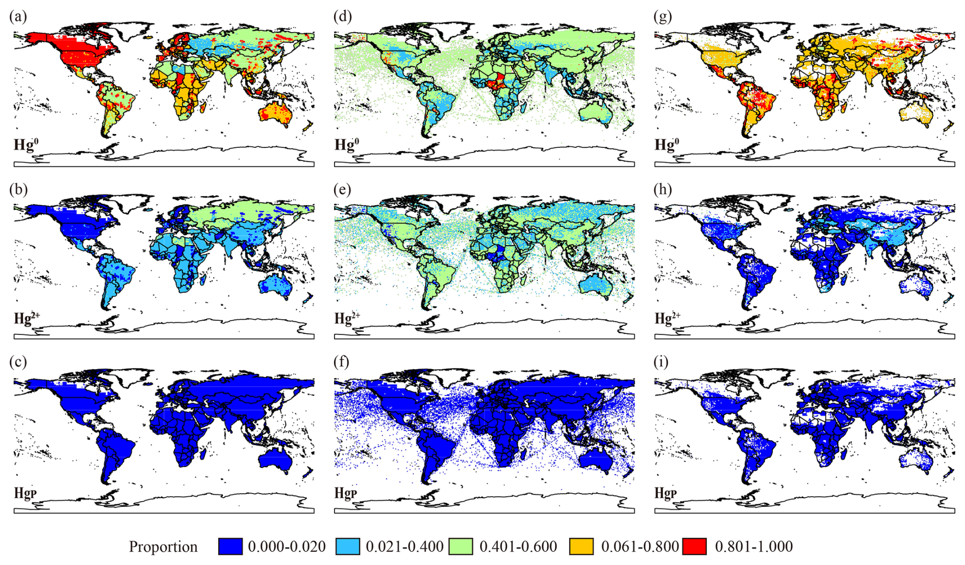
Figure 5The proportion of speciated Hg emissions in the total emissions by grid: the (a–c) STREETS dataset 2010 (Streets et al., 2019b), (d–f) EDGAR dataset 2010 (Muntean et al., 2018), and (g–i) AMAP/GMA 2010 dataset.
Emission inventories for MCHgMAP simulations
The MC was signed in 2013 and entered into force in 2017. To evaluate the effectiveness of the MC, the proposed timescale for the emission inventory should cover at least the 2 years mentioned above. As discussed above, currently, several global anthropogenic Hg emission inventories are available for 2010, and two inventories are available for 2015 (AMAP/GMA and STREETS). Given that UNEP launched the negotiations on a global mercury instrument in 2009 and actions have been taken since the convention's negotiations by some parties, using 2010 as the starting year for the EE analysis is recommended for MCHgMAP simulations. Furthermore, an extension of current Hg emission inventories to at least 2020 is recommended for analyzing the effects of changes in anthropogenic Hg emissions as a result of the MC on environmental Hg levels using model simulations. However, it should be noted that 2010 may be an anomalous year in the longer time trend of Hg emissions, as it was probably affected by lower activity levels following the global economic downturn in 2008, as may also be the case in 2020 due to COVID-related economic impacts.
The EDGAR global anthropogenic speciated mercury emission inventory is planned to be extended until 2022. It will provide emission time series for all of the world's countries at 0.1×0.1° resolution for the period 1970–2022 together with a comprehensive trend analysis by sector and regional or top emitter, including the impact of the pandemic on mercury emissions. The updated EDGAR mercury inventory release, based on EDGARv4.tox2 (Muntean et al., 2018) mercury emissions for the period 1970–2012, is primarily focused on updating the global mercury emissions for the last decade. However, in the case of the availability of new and better input data sources, activity data in particular, the EDGAR emissions will be updated retrospectively as well. The technologies and end of pipe, for the power generation sector in particular, are from the new edition of the Platts database, except for China, for which the information in Zhang et al. (2023b) is used. EDGAR emission time series are aggregated using both IPCC 2006 and IPCC 1996 classifications for each country. The revised EDGAR Hg inventory release will also provide global monthly sector-specific gridded emissions. Regarding the spatial distribution, the proxy data for point, linear, and areal sources are planned to be updated continuously in EDGAR, and thus the new version of the EDGAR Hg emissions will benefit from the latest updated proxy data. For example, the new population proxy used in EDGAR is based on the JRC GHSL (https://ghsl.jrc.ec.europa.eu/https://ghsl.jrc.ec.europa.eu/, last access: 1 May 2025), which combines the latest population census data (CIESIN GPWv4) with satellite imagery of built-up areas (Landsat 8). Speciation of mercury emissions will be based on the literature review presented and evaluated in Muntean et al. (2018) through model simulations using the GEOS-Chem mercury model, including nested simulations and comparison with measurements. In addition to mercury emissions, EDGAR (a multipurpose and independent global database) also provides consistent emissions of greenhouse gases (GHGs), unintentional persistent organic pollutants (UPOPs), and air pollutants (APs).
Plans are also under consideration for updating AMAP/GMA 2015 emissions to 2020 estimates for at least some parts of the inventory based on the AMAP/GMA methodology, and they potentially provide estimates for the intervening years since 2010.
Limitations of available emission inventories and recommendations
As presented above in this section, Hg emission inventories compiled by different groups varied in source classification, emission amounts, inventory compilation, spatial distribution, and Hg speciation profiles. Therefore, when using existing emission inventories for temporal trend modeling, it is necessary to ensure the comparability of emission inventories over the time period considered. Even if the emission inventory was compiled by one group, the emission data from different years may not be fully comparable due to changes in emission estimation methods, the sectors included, or, e.g., the sources of the activity data used. Inventories are in some cases only prepared at intervals (typically 5-years), so annual estimates would involve interpolation.
The EDGAR dataset (1970–2012) annual estimates are internally comparable, and gridded speciated Hg emission inventories by sector are publicly available. Currently, the emission amounts estimated in EDGAR are significantly lower than those estimated in other emission inventories, especially for the earlier part of the period. The AMAP/GMA emission inventories for 2010 and 2015 are consistent and comparable due to consistent compilation methods; the emission sectors addressed in 2010 were updated in connection with the work on the 2015 inventory. However, the AMAP/GMA gridded data for 2010 and 2015 apply the same (2015) spatial distribution proxies and point source information and therefore do not reflect any changes in these between 2010 and 2015. The advantage of the STREETS dataset is its centennial-scale coverage. However, to achieve such a long-term emission dataset, the spatial resolution and the fineness of the emission source classification have been more or less sacrificed. In addition, the emission factor changes over time were generated based on a transformed normal distribution function. Therefore, the accuracy may be impacted to some extent when using this method to evaluate the effectiveness of the control measures.
The gaps in understanding Hg speciation profiles in emissions to the atmosphere are considered to be the largest uncertainty source of speciated Hg emissions. The criteria used to determine the speciation profiles have varied in different inventories. For example, the WHET datasets recommended that the emission profiles for coal-fired power plants be for Hg(0) : Hg(II)g : Hg(II)p based on the assumption that oxidized Hg will be reduced to Hg(0) in the smoke plume. It is important to also recognize that improving information on speciation associated with different control technologies is only part of the puzzle. A further complication (and probably more important when it comes to developing inventories for tracking changes over time) concerns the extent to which different technologies are applied in different countries and (if possible) individual facilities and how this has changed over time. Speciation of ASGM emissions is an area requiring particular attention. The AMAP/GMA inventories assume that all ASGM emissions are in the form of Hg(0) (i.e., the form evaporated when heating an amalgam). It is therefore assumed that any subsequent oxidation to Hg(II) species is not an intrinsic part of the “emission” profile associated with the ASGM process but would need to be addressed in the modeling (as part of the air chemistry), even if, due to emissions at the ground level, this may take place very soon after emission due to interaction with, e.g., vegetation or surfaces. Furthermore, the global dispersion and deposition of Hg are seasonally dependent. Some information is available on the seasonal distribution of Hg emissions from regional inventories, but current global inventories provide no such information. The seasonal distribution of anthropogenic emissions depends on the sectoral distribution; therefore, it is likely to vary spatially and possibly change over time as emission controls are applied to various sectors. In addition to specific Hg control measures, air pollution control devices aimed at removing SO2, NOx, PM2.5, or dioxins can also synergistically remove Hg. Therefore, consideration of changes in fuel use driven by economic factors or pollution control and climate change mitigation policies is important for attributing the observed changes in Hg emissions and environmental levels over the MC–LRTAP “effectiveness” analysis period.
One of the key questions of EE is to address whether the measures taken have changed Hg emissions, releases, and usage. Therefore, to evaluate the impact of control measures, the mass flow approach (i.e., tracking mercury mass from sources through various stages of a given human activity process to its final emission or release into the environment; Hui et al., 2017) is the most suitable method for application. By using this method, the Hg removal effect of control measures can be quantified. To promote EE cycles, mass flow approaches should be applied for emission inventory compilation. To understand the impact of future emission reductions on the environment and humans, control-measure-specific Hg speciation profiles should be applied instead of sector-specific speciation profiles. Many field experiments have been conducted in the past 2 decades to characterize emissions, especially addressing exhaust flue gas emissions from large point sources. Although it can be argued that the information on speciation of emissions is very specific to measurements at a particular plant or facility, these studies provide an opportunity to improve the generic speciation schemes employed in global emission inventories. It is timely therefore to review existing field experiments, including the test methods, results, and facility information, and to develop new, standardized Hg speciation profiles based on pollution control device information to replace the existing speciation profiles applied in different emission inventories to date.
Where possible, the source classification criteria should be harmonized between inventories. Given that both air pollution control and measures to reduce carbon will impact Hg emissions, using consistent source classification criteria for sources which emit air pollutants, carbon, and Hg simultaneously is recommended. As for spatial distribution, distribution methods and the proxy applied should also be unified to ensure the comparability of different studies. Point source information should be used to the greatest extent possible to locate emissions for convention-related sectors: coal-fired power plants, coal-fired industrial boilers, cement clinker production, waste incineration, and nonferrous metal smelting (zinc, lead, copper, and large-scale gold production). Several data sources can aid in the compilation of point source emissions. First, according to the requirement of the MC, parties should compile the emission inventories of point sources before 2022 and update them periodically. This will provide information for future inventory compilation. Second, PRTR systems can be used to develop indicators for Hg emission point sources. Although the methods and reporting systems applied in a given country or system may differ from each other, facility information such as facility location will help to locate the calculated emissions. Third, the resolution and timescale of regional emission inventories have been improved in the past decade. The participation of national experts can help considerably in both the development of emission estimates and the compilation of gridded emission inventories that could be used to evaluate the effectiveness of control measures. Updating of global emission inventories prepared under the EDGAR and AMAP/GMA inventory initiatives should be continued and supported, including efforts to understand and reconcile the differences in historical emission estimates. Finally, the information applied to compile anthropogenic Hg emission inventories to support the MC should be transparent, reviewed, and fully documented.
3.2.2 Future emissions
Scenario modeling is a valuable tool for understanding the effects of different policies and abatement measures on future anthropogenic mercury emissions. For each scenario, Hg emissions are projected into the future based on a set of assumptions and projections of energy use, industrial activity, and macroeconomic development combined with a narrative on climate, air pollution, and mercury control policy. Such emission scenarios provide vital input for atmospheric models to assess the effects of mitigation policies on global Hg transport and deposition (see Table E6).
To project mercury emission inventories into the future, a large number of considerations need to be addressed and reconciled with available data sources for both present emissions and emission projections (see Table E7). Frequently, emission projections are based on trajectories of different economic activities linked to Hg emission and computed by integrated assessment and energy system models (e.g., IEA 2022; Chen et al., 2022). The future emission intensity of each sector is driven by activity levels, fuel mix changes, and the impacts of emission control measures. The activity projections can incorporate underlying assumptions about climate policy, creating the possibility of evaluating the co-benefits of different GHG mitigation strategies in mercury emissions. Furthermore, air pollution control policies for particulate matter (PM), SO2, and NOx can be distinguished from Hg-specific policies to identify where Hg reduction materializes due to co-benefits or direct Hg abatement. Scenarios of emission control strategies (i.e., the application rates of technical pollution control) are included in future global Hg emission projections, either implicitly or explicitly.
Overview of global and regional future emission scenarios
Tables E8 and E9, respectively, summarize global and regional future Hg emission scenarios published in the literature, including their base and last projection year, source of underlying activity and energy projections, and assumptions about Hg control measures, where applicable. The emission sectors covered by the published global emission projections are presented in Table E10.
Sectoral coverage
The sectoral coverage of the published global emission projections varies widely. The projections differ in the choice and level of detail of the anthropogenic emission sources by which the sectors are represented, as well as in their inclusion or exclusion of sectors such as biomass combustion (e.g., burning of crop residues or residential biomass combustion for cooking and heating), different industrial processes using Hg, and other sectors with unintentional emissions, such as iron and steel production or caustic soda and vinyl chloride monomer (VCM) production.
For the representation of power plants, industrial and residential combustion, some models account for different types, sizes, and ages of power plants, while others simply consider an average emission factor for all coal combustion processes. Similarly, emission factors of power plants vary depending on the quality and type of fuel, as well as fuel-trading patterns, which may change in the future. Industrial processes such as iron and steel making, cement production or nonferrous metal (NFME) production are also highly complex and may be aggregated or sub-divided into several processes, all with distinct Hg emission intensity. For example, copper, zinc, and lead are reported separately per metal in most Hg emission scenarios (Streets et al., 2009; Pacyna et al., 2010, 2016; Lei et al., 2014) but are aggregated with all other NFME in Rafaj et al. (2013). On the other hand, iron and steel production are separated into subsectors in some (Rafaj et al., 2013) but aggregated into one sector for other studies. Processes such as cement production, where it may be difficult to separate emissions from fuel combustion and those emitted from the raw materials, also require close attention. For the waste sector, activity projections need consideration of the changing Hg content in waste as intentional Hg use is phased out from different products. Some studies apply their own calculations regarding consumption of Hg-added products (e.g., Pacyna et al., 2016; Burger Chakraborty et al., 2013), while others assume an average Hg content in waste and the emission factor scaled to complete waste generation statistics (e.g., Rafaj et al., 2013).
Sources of energy projections
Various integrated assessment models for energy and activity projections have been used for energy-intensive emission sources, e.g., fossil fuel and biomass combustion and industrial activity and transport, as well as for activities driven by population growth, i.e., cremation. Frequent use has been made of climate pathways from IPCC reports, such as the IPCC Special Report on Emission Scenarios (IPCC, 2000; Streets et al., 2009; Lei et al., 2014; Giang et al., 2015) or the IEA World Energy Outlook scenarios (Zhao et al., 2015). Others have made use of regional energy models (e.g., ReMIX for Europe, Rafaj et al., 2014; C-REM for China, Mulvaney et al., 2020). Activities of sectors not covered by energy or integrated assessment models (e.g., ASGM, some Hg-specific sectors such as chlor-alkali production, cremation, generation of mercury-bearing wastes, and VCM production) are derived from other sources and drivers. For the waste sector(s), Chakraborty et al. (2015) considered the buildup of stocks of mercury-added products and its delay in entering the waste system.
Emission controls
Lei et al. (2014) use implicit assumptions about emission control technologies, while others include explicit emission control strategies (Rafaj et al., 2013; Ancora et al., 2016; Pacyna et al., 2016; Wu et al., 2018b). Most scenarios compare a base case, such as a “current legislation” (CLE) scenario, to the maximum technologically feasible reduction of Hg (HgMFR). Air pollution control policies for PM, SO2, and NOx can be distinguished from Hg-specific policies to identify where Hg reduction materializes due to co-benefits or direct Hg abatement. In well-studied sectors like coal combustion or industrial processes like cement production or iron, steel, and NFME production, a range of pollution control options, mostly relating to co-benefits from installing PM, SO2, or NOx control technologies (Rafaj et al., 2013; Ancora et al., 2016; Pacyna et al., 2016; Wu et al., 2018b), may be applied to divert Hg emissions to the air into solid or liquid waste streams. In other sectors, the applied measures may be more qualitative, such as good practices, bans on activities, improved storage and handling, or an assumption about the decreasing emission intensity of an activity, without explicit reference to a control measure. Mercury-specific control technologies are also entering the market. While they are not widely applied at the current moment except for very specific applications (e.g., cleaning of H2SO4 from acid plants, waste incinerators, and selected coal power plants), they may become more prominent in the future. The best-documented CLE control strategy for Hg can be found in the GMA 2018 (AMAP/UN Environnement, 2019), where assumptions about technology efficiency and application for the year 2015 were applied to each sector–activity combination and each country – however, no assumptions about future technology applications are included in this document.
Scenario time period and resolution
Available future emission scenarios also differ in their chosen base and projection years, whether projections are available over the time series or for 1 endpoint year, and whether emissions are spatially distributed or aggregated. The GAINS model produces emission projections in 5-year steps from 2010 to 2050, but Pacyna et al. (2016) and Streets et al. (2009) only project the last years, i.e., 2035 and 2050, respectively. While Pacyna et al. (2016) and Streets et al. (2009) provide gridded emissions, Hg emissions from GAINS are not spatially distributed yet.
Formulation of future emission scenarios
Currently available published future emission scenarios of Hg are mostly projected based on 2010 inventories or older data on anthropogenic emissions. Several atmospheric modeling studies have estimated future Hg transport and deposition based on these projections (e.g., Schartup et al., 2022). It is recommended that the new modeling assessment of the future emission scenarios be conducted by starting projections from the 2015 emission inventories, the most recent year of currently reported anthropogenic emissions. Presently, two such efforts are ongoing that are aimed at producing up-to-date future global Hg emission scenarios, as summarized in Table E11:
- i.
An update of the Hg implementation in the most recent version of the Greenhouse Gas–Air Pollution Interactions and Synergies (GAINS) model (http://gains.iiasa.ac.at/models/gains_models4.html, last access: 1 May 2025) at the International Institute for Applied Systems Analysis (IIASA) (Amann et al., 2011). The updated model is calibrated to GMA 2018 emissions, using 2015 as the base year, with a mixture of the most up-to-date emission factors derived from GMA 2018 and supplemented by regionalized emission factors derived from coal Hg content and trading patterns. The update also includes the introduction of the full range of Hg-specific control options for all relevant sectors and extends the calculation to co-benefits from PM and SO2 control policies in the model. Activity data input stems from different global and regional statistics and energy system models, notably the World Energy Outlook Scenarios which are published annually by the IEA and are implemented fully in the modeling framework. GAINS is freely available to the public, although access to Hg emissions is currently restricted due to ongoing development. Hg-GAINS 4 has been fully functional since December 2023, and publication of the first results is in progress.
- ii.
Future Hg emission scenarios are being added in the Tool for Air Pollution Scenarios (TAPS) model (Massachusetts Institute of Technology (MIT); Joint Program on the science and policy of global change) in collaboration with the Italian National Research Council, Institute of Atmospheric Pollution Research (CNR-IIA), and European Commission Joint Research Council (JRC). TAPS is a flexible and public tool that enables users to combine and study a wide range of future emissions under strategic climate objectives and air pollution control policies, using the most up-to-date emission factors (Atkinson et al., 2022). It can efficiently assess a wide range of climate and air quality policy pathways – from broad to specific at the regional, sectoral, and fuel-based levels. TAPS has three components: historical global anthropogenic emission inventories, activity data for future scenarios from the MIT Economic Projection and Policy Analysis model (EPPA) (Chen et al., 2022), and emission intensity trends based on recent scenario data from the GAINS model. Spatially gridded emission outputs can be used as input variables in chemical transport models (CTMs). The Hg extension in TAPS will calculate Hg emission projections by combining the EDGAR Hg inventory, EPPA climate policy scenarios, and time-dependent Hg emission factors derived from different future Hg emission scenarios (Atkinson et al., 2022; Chen et al., 2022).
Updated future emissions should include a set of scenarios spanning policy-relevant conditions from no additional control, technical scenarios based on Hg control policy and co-benefits from other air pollutant abatement, and a range of plausible scenarios on climate pathways. A selected list of scenarios is outlined in Table E12. The output should be spatially gridded emissions per sector and region up to 2050 or beyond. This full set of requirements is to be available in the future in both GAINS v4 and TAPS.
There are several limitations in projecting Hg emissions into the future. Accuracy of future emission scenarios is limited by the large uncertainties in Hg emissions in many sectors such as waste or ASGM. Many available Hg control technologies are still not widely used, as their cost is prohibitively high for many industrial applications. Cost considerations are not (yet) included in this modeling plan but are in development by different research groups. Furthermore, assumptions are made about future emission control technologies, their efficiency, and their impact on emission speciation. As data are scarce for such technologies, large uncertainty within speciation profiles of future emissions occurs. The future spatial distribution of emissions is also important, e.g., for modeling Hg deposition, but it may be hard to project depending on the location of future Hg emission sources. Furthermore, the emission intensity of emission sources in different regions might change over time in complex ways: trading patterns of fuels and ores with varying Hg contents may shift or technology learning may lower emission factors of a particular emission source in a particular region.
3.3 Wildfire re-emissions
The uptake of gaseous elemental mercury (Hg(0)) by plant stomata represents the major global sink of Hg from the atmosphere to terrestrial systems (Zhou et al., 2021; Feinberg et al., 2022). Combustion of Hg containing vegetation has the effect of reducing oxidized forms of Hg and releasing the highly volatile Hg(0) into the atmosphere (Biester and Scholz, 1997; DeBano, 2000; Biswas et al., 2008). Therefore, it is critically important that we can produce constrained estimates of Hg emissions from wildfires, particularly with predicted increases in fire frequency and intensity associated with climate-change-driven extreme weather events (McKenzie and Kennedy, 2012; Walker et al., 2019).
Without question, the greatest obstacle to the development of effective Hg wildfire emission modeling is the scope (or lack thereof) of existing observational data (De Simone et al., 2017b; Fraser et al., 2018; McLagan et al., 2021). From our review of the literature, there are only five near-source data sources (i.e., measurements taken <100 km from fires): (1) Brunke and Labuschagne (2001) – ground-based measurements of a fynbos shrubland fire at Cape Point, South Africa; (2) Friedli et al. (2003a) – aircraft-based measurements of a boreal forest fire in northern Ontario, Canada; (3) Friedli et al. (2003b) – aircraft-based measurements of a temperate forest fire in Washington State, USA; (4) McLagan et al. (2021) – aircraft-based measurements of a boreal forest fire in northern Saskatchewan, Canada; and (5) Desservettaz et al. (2017) – ground-based measurements of northern Australian savanna fires. Hg accumulation rates within vegetation vary by a factor of ≈25 across the different species and biomes. Accordingly, Hg concentrations in biomass also vary considerably by biome, vegetation type, and tissue type (Zhou and Obrist, 2021). With the existing data limited to a few biomes, large assumptions (and the associated high uncertainties) are required to estimate wildfire emissions of Hg across broad spatial scales.
All other studies that have examined Hg emissions from wildfires have involved large source–receptor distances, and the emission ratios (ERs; ratios of concentration enhancements between Hg and a reference species, typically Hg(0) : CO – carbon monoxide) of these studies are elevated compared to those of the four near-fire studies (for a summary of these data, see Wang et al., 2015, and McLagan et al., 2021). McLagan et al. (2021) highlight the concerns associated with large source–receptor distances and with the differing atmospheric lifetimes of Hg(0) and reference compounds (i.e., CO). While ERs can be used to produce estimates of wildfire emissions by simple conversions of emission estimates of the reference compound at the scale of interest (single fire, regional, global biome, or total global emissions), this method is highly uncertain and full uncertainties are difficult to characterize (BE1) (McLagan et al., 2021). EFs quantify the unit mass of the target species (i.e., Hg(0)) released per unit mass of fuel combusted and are the preferred empirical method used to generate emission estimates. Hg EFs require an enhanced (above-background) mixing ratio data of Hg (Hg(0), Hg(II)p, and/or Hg(II)g) and the major carbon species emitted from fires: CO, carbon dioxide (CO2), methane (CH4), and non-methane organic gases (NMOGs). Friedli et al. (2003a, b) measured CO and/or CO2 and derived the Hg EFs from their respective fires using an assumed ratio of for CO2, CO, CH4, and NMOGs. However, the study by McLagan et al. (2021) measured all four carbon species and determined a ratio of (). The ratios of these co-emittants matter for the estimation of Hg emissions from wildfires, and (where possible) they should be measured in tandem with Hg species when assessing Hg releases from wildfires.
Data are limited further by the fact that the one near-source study (Friedli et al., 2003b) that did measure particulate-bound Hg used a less robust bag collection system with ex post facto laboratory analysis (Hg(II)p). Furthermore, none of these near-source studies has measured gaseous oxidized mercury. While it is assumed that any Hg(II)g species formed within wildfire plumes would rapidly partition into the abundance of wildfire-released particulates and aerosols, as evidenced in laboratory burns (Obrist et al., 2008), there are no field data to validate this assumption. Previous modeling efforts have utilized the 3.8 % fraction of Hg(II)p (out of total atmospheric Hg: Hg(0) + Hg(II)p + Hg(II)g) that was measured in the Washington State fires (Friedli et al., 2003b) with the addition of other (assumed) Hg(II)p ratios (up to 50 % Hg(II)p) to provide sensitivity analyses (De Simone et al., 2017b; Fraser et al., 2018; Kumar and Wu, 2019; McLagan et al., 2021). However, we have little to no knowledge of how the ratio of Hg(II)p to Hg(0) might vary by biome or fire intensity. The atmospheric lifetimes of Hg(II)p and Hg(II)g are much lower than Hg(0); altering the fraction of Hg(II)p released results in large increases in local and regional Hg deposition (De Simone et al., 2017b; Fraser et al., 2018; Kumar and Wu, 2019). Full atmospheric Hg speciation measurements within wildfire plumes are desperately needed to constrain the fraction of Hg(II)p (and potentially Hg(II)g) released from wildfires, and how this varies by fire intensity, vegetation type, meteorology, and duff conditions will be critical for improving estimates of Hg emissions from wildfires.
Due to the conversion of Hg(II) into Hg(0) at temperatures observed in fire, we assume complete volatilization of Hg from combusted biomass. However, this is not an assumption that can be made down whole soil profiles, which are a major storage pool of Hg within vegetated ecosystems (Schwesig and Matzner, 2000; Friedli et al., 2007; Obrist et al., 2012). The fraction of Hg that will be released from soil depends on the temperature the soil reaches during a fire, which in turn is dependent on fire intensity and soil properties (i.e., texture, initial water content, chemical properties, water repellency, wet aggregate stability, and soil organic matter content) (Stoof et al., 2010; Mataix-Solera et al., 2011; Martínez et al., 2022). More data on Hg releases from laboratory-controlled burns that include reconstructed soil profiles and pre- and post-fire site assessments of soil profile Hg mass balances would be greatly beneficial for characterizing the contribution of Hg released from soil when modeling Hg releases from wildfires. “Bottom-up” approaches that utilize soil + biomass Hg concentrations to estimate EFs and total Hg emissions from fires do exist (Biswas et al., 2007; Cinnirella and Pirrone, 2006; Turetsky et al., 2006; Engle et al., 2006; Woodruff and Cannon, 2010), and many of these are incorporated into the Hg EFs for the different biomes provided by Andreae (2019). However, compared to the near-source, aircraft-based, and top-down EFs in boreal and temperate forests (Friedli et al., 2003a, b; McLagan et al., 2021), it would appear that most of the bottom-up methods also overestimate EFs (and consequently Hg emissions) from wildfires by a factor of 3.1±2.7 for these biomes (based on the studies listed in the previous sentence).
The interannual variability in the burned area of wildfires, both between and within different ecosystems, can be vast due to the complexities of factors that control large-scale wildfires (de Groot et al., 2013; Clarke et al., 2019). The magnitude of this variability is related to the fire return interval, fuel load, meteorology, forest composition, and longer-term trends in the climate (i.e., seasonal, annual, and decadal) that drive drought or flood cycles (de Groot et al., 2013). Moreover, there is large variability between the remote-sensing-based biomass burning emission products (i.e., GFED, FINN, GFAS, QFED, and FEER) used to estimate spatially and temporally varied distributions of burned area and the mass of fuel burned, with very large differences shown between the inventories on regional and global scales (Giglio et al., 2013; Forkel et al., 2019; Humber et al., 2019; Pan et al., 2020). This highlights the uncertainty of remote sensing estimations of burned area and burned fuel at the coarser resolution typically used for global estimates – many small fires are missed at this spatial scale, and small fires make up the majority of the total number of fires that occur (Ramo et al., 2021).
Existing global emission estimates incorporate many of the uncertainties and limitations discussed in the previous section, and hence they have large uncertainty terms that may not include all or fully propagated uncertainty components (McLagan et al., 2021). Friedli et al. (2009) estimated global wildfire emissions at 675±240 Mg yr−1 using biome-specific wildfire EFs (based on large assumptions), and Kumar et al. (2018) produced an estimate of 612 Mg yr−1 (no overall uncertainty provided) using a similar method, albeit with some adjustments to certain biome-specific EFs. De Simone et al. (2017b) produced an alternate estimate of 400 Mg yr−1 (no overall uncertainty provided). All of these estimations include the mean of all measured ERs or EFs, including in studies with bottom-up approaches and studies with large source–receptor distances, with the exception of the most recent and robust study examining wildfire emissions (McLagan et al., 2021) that was published after all previous modeling efforts. ERs and EFs in these studies are all considerably larger than the values determined from near-source measurements (McLagan et al., 2021), which has likely resulted in an overestimation of wildfire emissions. This is highlighted by contrasting the emission estimate made for all boreal forests by McLagan et al. (2021) (18±14 Mg yr−1, based on near-source measurements of a boreal forest wildfire) to the Kumar et al. (2018) estimates for boreal forests (≈200 Mg yr−1, including EFs measured at large source–receptor distances and bottom-up assessments), which differ by an order of magnitude.
3.3.1 Formulating wildfire emissions
Logically, this and future modeling efforts should use the 14 fire regions typically utilized by biomass burning emission products as the basis for the different biomes that should be assessed. For MCHgMAP, wildfire Hg emission estimates will be developed using the latest GFED4 and FINN2 biomass burning products (both products allow EF inputs rather than the more uncertain ER approach); the inherent variability between these products' estimates will provide enhanced uncertainty assessment and model sensitivity to the critical burned area and burned fuel amount parameters for the years 2010–2020. EFs for each biome will be taken from Andreae (2019). As discussed, bottom-up approaches and studies with large source–receptor distances likely overestimate EFs in temperate and boreal biomes. Thus, we plan to utilize the mean value of EFs from the three “top-down”, near-source, and aircraft-based studies ( g kg−1; Friedli et al., 2003a, b; McLagan et al., 2021) for temperate and boreal biomes. Lacking near-source EF data for other biomes (grassland or savanna, tropical forests, and croplands), we will use the EF estimates from Andreae (2019), unadjusted. Additionally, we will apply a range of Hg(II)p fractions (out of the total atmospheric Hg emitted), ranging from 0 % (100 % Hg(0) emissions) to 25 % Hg(II)p.
3.3.2 Limitations and recommendations
While we anticipate this assessment of global Hg emissions from wildfire will represent the best assessment to date, large uncertainties and limitations remain. First and foremost is the very large (and difficult to fully assess) uncertainties of EFs applied to the 14 global fire regions. The good agreement between the calculated EFs for the three aircraft study from wildfires in boreal North America and temperate North America lead us to conclude that the applied EFs based on these studies are the most constrained biome-specific EFs available. How well these values apply to similar fire regions such as Europe or boreal Asia we cannot accurately estimate without further in-depth study. Moreover, EFs for other biomes are highly uncertain; they are based on highly variable data and include estimates from very different ecosystems (i.e., EFs for savanna/grasslands/shrublands vary by close to 2 orders of magnitude and include estimates from South African fynbos shrubland, South African Savanna, Mediterranean shrubland, Australian savanna, and Nevada (USA) brushland). Generalising highly variable EFs for such broad and variable ecosystems/biomes is a clear limitation of past studies and remains so for any estimates generated from this work. Future work should focus on (1) expanding the number of measurement-based EF estimates we have available (i.e., more near-source, top-down estimates), and/or (2) examining methodologies to adjust and constrain these biome-specific EFs using proxy data from more spatially and ecosystem diverse measurements/estimates such as species- or ecosystem-specific biomass Hg concentrations or accumulation rate data (Feinberg et al., 2022). Future efforts to improve on the rather limited top-down measurements should also look to include speciated atmospheric Hg measurement. As stated, the fraction of Hg(II)p emitted has a substantial impact on local re-deposition vs. long-range transport potential of the emitted Hg. With so few speciated atmospheric Hg data measured from wildfire plumes in the literature to date, this adds uncertainty not only to the estimates of Hg emitted from wildfires, but also to the cycling and fate of that Hg after it is emitted.
3.4 Soil re-emissions
Mercury emissions from natural surfaces include the evasion of Hg derived from primary geogenic sources (e.g., Hg release from rock-weathering processes) (see Sect. 3.1) and legacy Hg stored in the terrestrial surfaces from historic atmospheric deposition and land releases. Re-emissions (or secondary emissions) of legacy Hg from the terrestrial biosphere are an important source of emissions of Hg. Global Hg(0) re-emission from terrestrial ecosystems has been estimated to range from 1000 to 2500 Mg yr−1 (Pirrone et al., 2010; Agnan et al., 2016; Outridge et al., 2018), based on scaling-up from field flux measurements. The relatively high uncertainty of this natural Hg emission limits the understanding of global and regional Hg cycling budgets (Pirrone et al., 2010; Wang et al., 2014b; Song et al., 2015). Using air–surface exchange models is another approach to estimating Hg re-emission from terrestrial ecosystems. In contrast to scaling-up of field measurements, the air–surface exchange model is based on parameterization of physicochemical factors that influence Hg re-emission fluxes at various temporal and spatial scales.
Two categories of modeling approaches have been applied to estimate Hg re-emissions from soil surfaces. Table 1 lists the modeling approaches reported in the literature. One is the regression-based scheme that relates emission flux to time-dependent environmental factors (e.g., soil Hg, temperature, and solar radiation) (Xu et al., 1999; Bash et al., 2004; Lin et al., 2005; Gbor et al., 2007; Selin and Jacob, 2008; Shetty et al., 2008; Smith-Downey et al., 2010; Eckley et al., 2016; Khan et al., 2019). These statistical relationships were obtained from controlled experiments that measure air–soil exchange fluxes subject to changes in air and soil Hg concentrations, soil moisture and organic content, air and soil temperature, solar irradiance, and other site-specific parameters. Since the soil flux data were collected at a limited number of sites and durations, such regression-based schemes may not be generally applicable across the globe because of existing data gaps in site-specific characteristics and the heterogeneous nature of soil surfaces.
Table 1A comparison of natural surface mercury flux models, extended from a previous review in Zhu et al. (2016) and summarizing data from the literature (Xu et al., 1999; Bash et al., 2004; Shetty et al., 2008; Gbor et al., 2006; Zhang et al., 2009; Bash, 2010; Wang et al., 2014b; Wright and Zhang, 2015; Selin and Jacob, 2008; Lin et al., 2010; Kikuchi et al., 2013; Eckley et al., 2016; Khan et al., 2019).
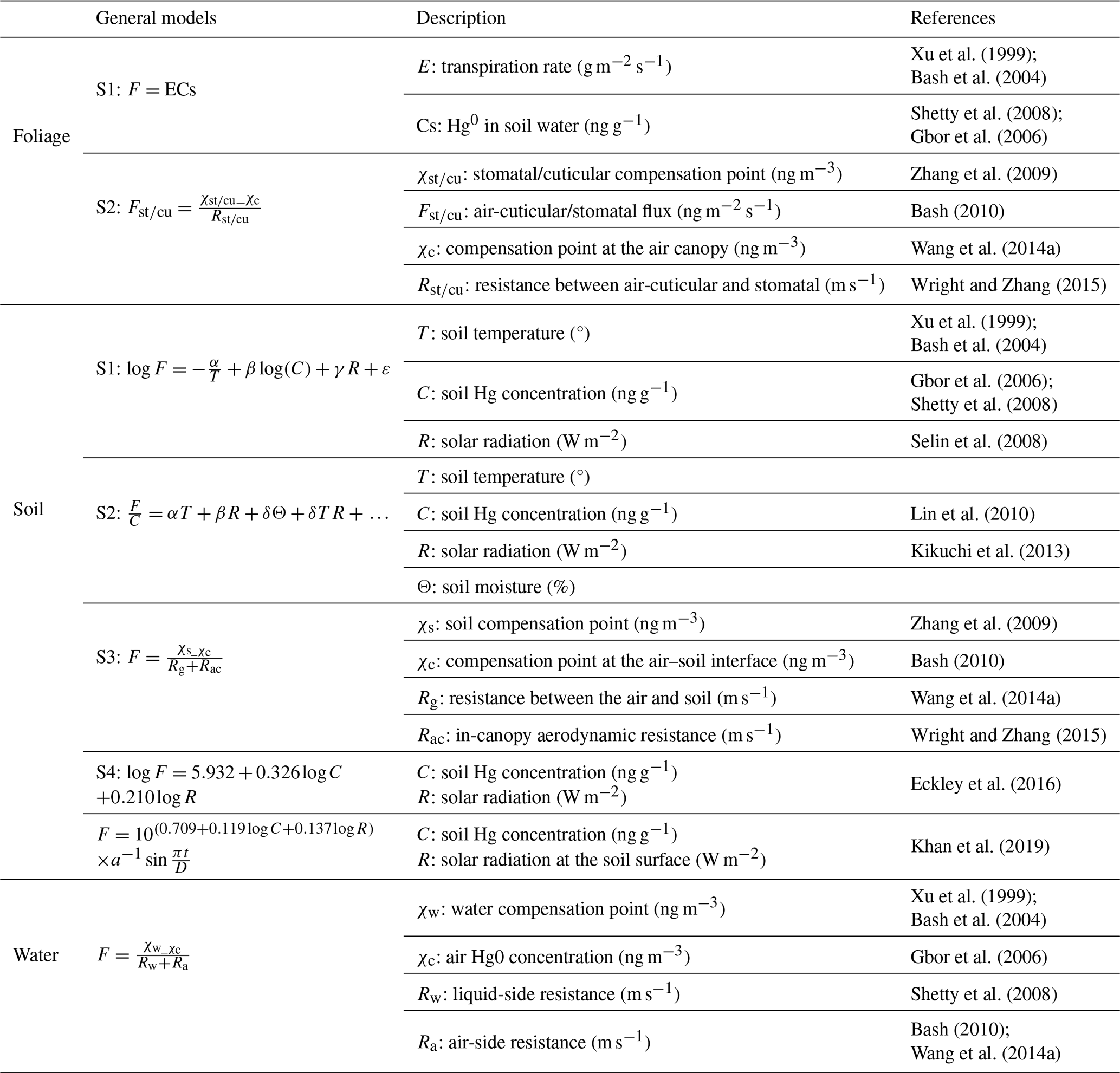
The other approach is the bidirectional flux scheme based on state-of-the-science understanding of Hg transformation in soil and on the cuticular surface under the influence of meteorological and environmental parameters (Bash, 2010; Wang et al., 2014b; Wright and Zhang, 2015; Wang et al., 2016b). This mechanistic approach depicts spatial soil flux variability more realistically and has the advantage of incorporating global land use data and model-generated meteorology in estimating the flux, although it is still limited by the availability of the required soil property data and other physicochemical parameters such as Hg(II) reduction kinetics and characteristics of interfacial exchanges (Bash, 2010; Wang et al., 2014b). Recent advances in the understanding of Hg(II) reduction kinetics provide new opportunities to enhance existing air–soil exchange modeling schemes. These include the constrained 10−11 to 10−10 s−1 pseudo-first-order rate constant of Hg(II) reduction in soil (Scholtz et al., 2003; Qureshi et al., 2011) and the 0.2–1.0 h−1 rate constant in natural water (O'Driscoll et al., 2006; Qureshi et al., 2010). In these reactions, the UV band of actinic light has been shown to be an important driver of Hg(II) photoreduction in soil and water (Moore and Carpi, 2005; Si and Ariya, 2011). The role of functional substructures (e.g., -COOH, -SH, and -OH) of dissolved organic matter during photoreduction has been determined by kinetic studies using model compounds (Si and Ariya, 2011, 2015; He et al., 2012). In dry soil, the first-order rate constants of Hg(II) photoreduction are 0.007–0.028 h−1 for HgCl2 coated over sand and 0.003–0.006 h−1 for Hg(II) in a natural soil (Quinones and Carpi, 2011). In the absence of light, Hg(II) reduction in soil is also observed at a rate of 0.001–0.002 h−1 at 293 K (Pannu, 2013).
Parameterization of Hg re-emission from natural surfaces in global Hg models has primarily used the regression-based schemes in the form F=aCbRc (where C is air concentrations and R is resistance). For example, the GTMM simulates Hg(0) soil emissions using soil Hg concentration (C) and selected environmental parameters, including temperature, solar radiation, and leaf area index (Smith-Downey et al., 2010), with re-emission fluxes coupled to the global chemical transport model (e.g., GEOS-Chem-Hg) and other Earth system model components (Zhang et al., 2021b; Zhang and Zhang, 2022). This modeling methodology requires relatively few readily available parameters for estimating spatially and temporally resolved re-emissions but does not account for the heterogeneities of the air–surface interface and the interplays between multiple environmental factors. Recent implementation of soil chemistry and kinetic parameters in bidirectional resistance schemes had been demonstrated for regional modeling (e.g., Bash, 2010; Wang et al., 2016c). Wang et al. (2016c) applied their mechanistic bidirectional terrestrial flux model and updated soil Hg data to estimate 565.5 Mg yr−1 of emissions from soil and 100.4 Mg yr−1 uptake by vegetation in China, improving previous estimates and spatial distributions (Shetty et al., 2008). The revised Hg air–surface exchange quantity as well as its spatial and seasonal patterns agree favorably with the measured fluxes at field sites in China.
Field measurements suggest that soil Hg concentration and solar irradiance are the dominant driving factors in Hg evasion from bare land and polluted soils, while other factors can influence the Hg fluxes to various degrees, depending on the environmental conditions at the measurement sites (Carpi and Lindberg, 1997; Lindberg et al., 2007; Gustin et al., 2008; Agnan et al., 2016; Zhu et al., 2016). Therefore, data on Hg concentration in the topsoil are essential for reliable estimates of Hg re-emission from soils in various ecosystems. Efforts to quantify global soil Hg concentrations have been made through empirical modeling, such as the Hg carbon ratio, linear regression, and nonlinear models, with the estimation of 240–1100 Gg Hg stored within the top 20 or 30 cm of soil layers worldwide (Liu et al., 2023; Smith-Downey et al., 2010; Wang et al., 2019). These estimates are, however, associated with large uncertainties since the spatial variability of soil Hg is controlled by multiple natural factors such as climate conditions, soil physiochemical properties, primary productivity, and anthropogenic activities (Ballabio et al., 2021). In general, most global soil Hg models lack adequate representation of Hg-contaminated regions and do not include a comprehensive set of parameters that influence air–soil exchange fluxes because measurements often only provide a subset of the parameters (Guo et al., 2024; Wang et al., 2019). Extensive topsoil Hg surveys in China, the USA, and Europe analyzed factors that influence soil Hg concentration and spatial distribution and reported hotspots of soil Hg distribution (e.g., mining and industrial pollution regions) (Ballabio et al., 2021; Panagos et al., 2021; Olson et al., 2022; Wang et al., 2019). These assessments and measurements are valuable for developing and constraining models to attain a more representative estimate and distribution of the global soil Hg content. Currently, there is a general lack of mechanistic processes implemented in global Hg models for estimating air–vegetation–soil exchange, although spatially and temporally resolved dry and wet deposition of atmospheric Hg is calculated in the models using species-specific (for elemental, oxidized, and particulate Hg) deposition schemes. Modeling work to incorporate updated process representations using more recent observational data is needed (Eckley et al., 2016; Wang et al., 2016c; Khan et al., 2019).
For the MCHgMAP MME simulations (see Sect. 5), spatially and temporally varying high-resolution global soil Hg re-emissions for 2010–2020 will be developed based on the mechanistic bidirectional air–land Hg exchange model of Wang et al. (2014b, 2016c) using global soil Hg distributions (Wang et al., 2019) and spatiotemporally varying environmental physical conditions simulated by the GEM-MACH-Hg model (Zhou et al., 2021). Harmonized soil re-emissions will be considered the default option for the multimodel study, and sensitivity simulations will be performed using model-specific parameterizations of soil re-emissions. In addition, influences of long-term changes in Hg emissions from soils (reflecting historical changes in anthropogenic emissions) will be investigated using mass balance modeling (see Sect. 5.3).
3.5 Oceanic re-emissions
Ocean Hg re-emissions (or evasion) into the atmosphere are driven by a combination of Hg natural (geogenic) and anthropogenic sources. Oceanic evasion is a major source of Hg in the atmosphere. Therefore, the development of spatiotemporally resolved surface ocean Hg(0) concentrations and air–ocean exchange datasets that can be used as forcings for atmospheric and multimedia model simulations is important to the MCHgMAP EE objectives. As Hg emissions and removal of Hg from active biogeochemical cycling are not in equilibrium, the Hg concentrations in the world's oceans have slowly been increasing but with varying speeds, driven by their circulation times in different basins and at different depths (Amos et al., 2013). The lifetime of Hg at the ocean surface is less than a year after the Hg will either go into the atmosphere or be transported to deeper water layers (Soerensen et al., 2010). Atmospheric deposition and riverine inputs are external sources entering the ocean surface, but Hg from deeper ocean layers can also return to the surface waters due to, e.g., thermocline circulation and seasonal mixed-layer deepening (Soerensen et al., 2010). Thus, the ocean surface contains Hg that recently entered the ocean through deposition or river discharge and Hg that cycled in the ocean for decades to millennia before reaching the ocean surface again. In addition to naturally released Hg, oceanic Hg re-emissions therefore contain a large fraction of Hg originally emitted from anthropogenic sources, both recently and centuries ago (Amos et al., 2013; Outridge et al., 2018).
Oceanic Hg evasion, a diffusive process at the air–sea interface, results in the flux of Hg(0) across this interface. The gross diffusion is bidirectional, and the net direction of the flux is determined by the relative degree of saturation of the gas Hg(0) in water compared to the air concentrations (Soerensen et al., 2010). If the dissolved Hg(0) concentration in the surface water is undersaturated relative to equilibrium, the net Hg(0) flux is from the atmosphere into the ocean, and if Hg(0) is supersaturated, the opposite will occur. Both spatially and temporally, the surface ocean is thought to be supersaturated in terms of Hg(0) most of the time, resulting in a net flux into the atmosphere (e.g., Soerensen et al., 2013, 2014; Mason et al., 2017; Huang and Zhang, 2021). The supersaturation is caused by the continuous unidirectional input of other Hg species (mainly Hg(II)) through deposition and river input and the redox processes in the ocean resupplying the Hg(0) reservoir from that of Hg(II). The atmosphere–ocean Hg exchange is still largely unconstrained, with the estimated Hg(0) evasion ranging from 4800 to 8300 Mg yr−1, the Hg(0) deposition ranging from 1950 to 3900 Mg yr−1, and the Hg(II) deposition ranging from 2350 to 3900 Mg yr−1 (Sonke et al., 2023).
Recent advances in Hg isotope analysis are providing new insights into the relative contribution of gross Hg(0) and Hg(II) fluxes to the ocean (Jiskra et al. 2021). However, such observations are still limited, and it is not possible to determine the origin (anthropogenic or geogenic) or period of origin of the primary emission of Hg that are currently being re-emitted from the ocean based on traditional measurements of Hg concentrations (for an explanation of how the Hg(0) evasion flux is determined, see Sect. 4.4 and Appendix B). Both box and 3D models can be used to gain insights into the extent of the Hg(0) evasion flux from the ocean, the fraction that different sources or historical periods contribute, and how concentrations will change in response to changes in Hg ocean inputs as a result of measures under the Hg MEAs. Early box model estimates of gas exchange emissions from the ocean were initially quantified using limited data, primarily from the equatorial Pacific Ocean, as summarized in Sect. 4.4. These box models provided an early estimate of the relative change in emissions from the ocean due to anthropogenic impacts (e.g., Mason et al., 1994). Numerical models of ocean Hg gas exchange fluxes have been developed more recently. In the future, incorporating information on Hg isotope distribution and dynamics into the models will help provide a better constraint on the ocean evasion flux into the atmosphere.
For the MCHgMAP MME simulations, we propose developing spatiotemporally resolved surface ocean Hg(0) concentrations using ocean models as forcings for atmospheric models when calculating ocean re-emissions to the atmosphere (see Sect. 5.2 on 3D atmosphere and ocean simulations). Furthermore, we propose using atmospheric deposition estimates from atmospheric models to constrain the ocean models through the coupling approach described in Sect. 5.1. Currently, various 3D atmosphere and ocean models use slightly different parameterizations to calculate the air–sea exchange flux, but for the MCHgMAP a harmonized parameterization will be used to achieve consistency of ocean evasion flux as outlined in Appendix B.
Accurate determination of air–sea exchange fluxes is currently a major limitation for the simulation and analysis of environmental Hg cycling, given the limited observational data to constrain these estimates (discussed in Sect. 4.4: “Air–sea flux exchange”). The net flux determination also relies on the choice of gas exchange models, with current gas exchange models deviating especially for high wind speed estimates (Osterwalder et al., 2021). For recommendations on improving air–sea exchange estimates, see Sect. 4.4.
3.6 Riverine export
Rivers are important for ocean Hg concentrations due to their export of Hg, nutrients, and organic material into the coastal ocean. Accurate representation of the spatiotemporal distribution of the export of Hg, nutrients, and TOC (total organic carbon) from the terrestrial landscape to the ocean is needed to describe the ocean Hg levels and their environmentally driven changes. Riverine inputs include direct anthropogenic releases and Hg that has traveled through the terrestrial landscape for shorter or longer (centuries) periods, potentially being stored in the process (e.g., in permafrost) (Campeau et al., 2022). River inputs of Hg are controlled by both the water volume (which changes over time, e.g., due to climate change) and the Hg concentrations in the river discharge. Furthermore, as most of the riverine Hg discharge is in the particulate phase, the amount of total suspended solids (TSS) is also an important driver of riverine Hg discharge.
There are many studies of export from single rivers and river basins, and even global bulk estimates (Fig. 6). However, only a few global spatially resolved inventories have been assembled (Amos et al., 2014; Liu et al., 2021b). Amos et al. (2014) estimated river Hg export to be 5500±2700 Mg yr−1. The more recent study by Liu et al. (2021b) arrived at a lower estimate, with the input from rivers to coastal areas at 1000 (890–1220) Mg yr−1. Both studies estimated that ∼30 % (28 %–35 %) of river exports make it to the open ocean. Riverine inputs thus dominate in coastal areas (75 % of total inputs) and the Arctic (30 % – erosion being an additional source of deposition and river export in this area) but are less important in the open ocean (<10 %; Liu et al., 2021a; Dastoor et al., 2022a). The Liu et al. (2021b) inventory also, for the first time, estimated MeHg discharge (9656 (8405–11350) kg yr−1).
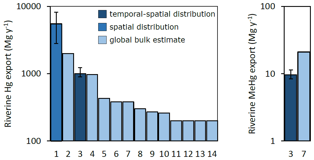
Figure 6Previously published riverine estimates for Hg and MeHg: (1) Amos et al. (2014), (2) Sunderland and Mason (2007), (3) Liu et al. (2021b), (4) Cossa et al. (1996), (5) Amos et al. (2013), (6) Mason et al. (2012), (7) Driscoll et al. (2013), (8) Outridge et al. (2018), (9) Semeniuk and Dastoor (2017), (10) Zhang et al. (2014b), (11) Mason et al. (1994), (12) Mason and Sheu (2002), (13) Fitzgerald et al. (2007), and (14) Selin (2014).
For the MCHgMAP simulations, we do not recommend any new development of river export schemes. Instead, the schemes for river discharge of Hg and environmental drivers (water volume, nutrients, and TOC) already integrated in the ocean models will be used (Table F6). However, we suggest a harmonization towards using the Liu et al. (2021b) Hg export inventory for all of the ocean models.
As seen in Fig. 6, there is still large uncertainty in the global riverine Hg export, with estimates from the past decade spanning from <300 to 5500 Mg yr−1 (Outridge et al., 2018; Amos et al., 2014). Only two studies have published a spatially resolved dataset that can be used in 3D model simulations, and these showed a factor of 5 difference in the total load. Furthermore, there is a lack of understanding of the temporal development of riverine export at the global scale. More studies on riverine Hg export resulting in spatially resolved export datasets should be conducted, with a focus on capturing temporal trends. The export range found in current publications should be narrowed down further in the coming years. While the end goal is a fully coupled ocean–land–atmosphere model, such datasets can be used to drive ocean models until the coupled models are developed and will be of great value for evaluating coupled models once these are developed.
Observational data may provide essential model inputs or a basis for comparison to and evaluation of model outputs. The following sections review the current availability of key observational datasets that may be useful for defining necessary model inputs or evaluating model outputs for a multimodel exercise. Specific methodologies for model evaluation are discussed in Sect. 6.
4.1 Air concentrations and wet deposition
The atmosphere is a key component of the Hg biogeochemical cycle, acting as a reservoir, an efficient transport mechanism, and a facilitator of chemical reactions. The chemical and physical behavior of atmospheric mercury determines how, when, and where emitted mercury pollution impacts Earth's ecosystems through deposition processes. To support the EE of the Minamata Convention, the guidance report UNEP/MC/COP.4/INF/12 recommends focusing on Hg(0) concentrations and wet deposition monitoring though automated, manual, or passive sampling. Monitoring of Hg(II)g and Hg(II)p is currently not prioritized for the EE due to analytical challenges (e.g., Lyman et al., 2010; Gustin et al., 2013; Jaffe et al., 2014; Huang et al., 2013). However, as noted in the guidance report, existing Hg speciation measurements can still be helpful in answering questions for the EE and can be used as first estimates.
Atmospheric Hg levels and Hg(II) wet deposition fluxes have been successfully monitored for decades through dedicated regional or global networks, including, e.g., the European Monitoring and Evaluation Program (EMEP; e.g., Tørseth et al., 2012), the US Atmospheric Mercury Network (AMNet; e.g., Gay et al., 2013), the National Atmospheric Deposition Program (NADP; e.g., Risch et al., 2017), the Canadian Atmospheric Mercury Measurement Network (CAMNet; e.g., Temme et al., 2007), the Global Mercury Observation System (GMOS; e.g., Sprovieri et al., 2016, 2017), more recently the South African Mercury Network (SAMNet), and the Asian-Pacific Mercury Monitoring Network (APMMN; Sheu et al., 2019). Hg(0) measurements primarily rely on automated active air sampling techniques, but the use of comparably inexpensive and easy-to-use passive samplers is becoming more common (e.g., McLagan et al., 2018b, 2019), progressively expanding the global coverage of atmospheric Hg(0) monitoring. The performance of passive samplers has been tested at several sites worldwide with satisfactory results (McLagan et al., 2018a). However, strict deployment and storage protocols must be followed to ensure collection of reliable results (Hoang et al., 2023). To support the MC EE, currently there is an ongoing effort to develop an overview of existing platforms managing monitoring of Hg levels in the air and to compile associated datasets which will serve as the basis for the MCHgMAP MME evaluation (see Sect. 6).
To constrain atmospheric chemistry in models, robust and high-temporal-resolution measurements of oxidized Hg (gaseous and particulate) concentrations and characterization of its chemical compounds under all environmental conditions are needed. However, currently deployed instruments for Hg(II) observations have significant artifacts (Gustin et al., 2021; Dunham-Cheatham et al., 2023). KCl-coated denuders, the predominant method for measuring Hg(II)g, have been shown to be biased low by up to 50 %; their collection efficiencies for various Hg(II) compounds depend on environmental conditions and local chemistry. Hg(II)p is typically collected on filters, such as quartz fiber and polytetrafluoroethylene (PTFE), which are found to also collect Hg(II)g. Recent advances in oxidized Hg measurement methods such as a dual-channel system (DCS) and a reactive mercury active system (RMAS) (Lyman et al., 2020a; Elgiar et al., 2024) allow for the development and deployment of new Hg(II) measurement systems in the field, which can improve the measurement accuracy and elucidate Hg(II) compounds involved in atmospheric chemistry across space and time. Gustin et al. (2024) recently reviewed the advances and limitations of current ambient Hg measurements and suggested that future work should focus on the development of the following: better surfaces for collecting oxidized Hg compounds, analytical methods for characterizing Hg chemistry, methods for differentiating between Hg(II)g and Hg(IIp, and high-time-resolution calibrated measurement systems.
Building on the existing literature, Sonke et al. (2023) provided a revised modern-day global Hg budget. The atmosphere is estimated to contain around 4 Gg of Hg, while the global total (wet and dry) Hg deposition to land includes 1600 Mg yr−1 Hg(II) deposition and 2850±500 Mg yr−1 Hg(0) deposition. It is worth mentioning that, despite current monitoring efforts, clear data gaps still exist, most notably in the Southern Hemisphere (Schneider et al., 2023). The advent of new analytical techniques, such as gradient or eddy covariance flux methods that allow whole-ecosystem net Hg(0) exchange measurements (e.g., Obrist et al., 2017; Osterwalder et al., 2016), will allow the scientific community to better constrain deposition fluxes and support the EE.
4.2 Air–land flux exchange
Air–land Hg vapor exchange fluxes have been reported at global and regional sites summarized in several studies (Agnan et al., 2016; Zhu et al., 2016; Eckley et al., 2016; Wang et al., 2016c). The Hg(0) flux data reported at global sites imply that vegetative surfaces act as net sinks of atmospheric Hg(0), while soil surfaces act as net sources of Hg for the air (Cooke et al., 2020; Grigal, 2003; Obrist et al., 2012; Zhou et al., 2020). Due to the diverse land surface characteristics and the limitations associated with the measurement methods, estimates of global air–land Hg fluxes remain highly uncertain. This section summarizes the observations of air–land exchange of Hg reported in the literature for model evaluation and provides recommendations for future studies. Observational data are invaluable for evaluating model performance and understanding how soil Hg exchange has varied historically and will change in the future.
Hg stored in vegetative biomasses originates primarily from uptake of atmospheric Hg, followed by assimilation in plant tissues. Mercury uptake by vegetation is the largest sink of atmospheric Hg in the terrestrial ecosystems (60 %–90 % of terrestrial Hg deposition), when aboveground biomasses are removed through litterfall, plant die-off (biomass turnover), and washout by precipitation (i.e., throughfall) (Zhou et al., 2021). Pathways of Hg uptake in vascular plants include uptake of atmospheric Hg via surface adsorption to foliage (Stamenkovic and Gustin, 2009), stomatal and/or cuticular uptake in foliage (Arnold et al., 2018; Greger et al., 2005; Peckham et al., 2019b), passive uptake to bark (Arnold et al., 2018; Chiarantini et al., 2016), and uptake from soils through roots (Greger et al., 2005; Juillerat et al., 2012; Laacouri et al., 2013; Obrist et al., 2012). Approximately 90 % of Hg in foliage is derived from uptake of atmospheric Hg(0) vapor, while the Hg in roots mainly originates from the soil uptake. Translocation of root Hg uptake from belowground to aboveground tissues in various plant species is limited (Yuan et al., 2022). Laboratory and field measurements confirm that foliage is a net sink of atmospheric Hg and that Hg accumulation in foliage is influenced by the air Hg concentration (Assad et al., 2016; Fay and Gustin, 2007; Millhollen et al., 2006; Niu et al., 2014); several studies including Hg stable isotopes suggest that stomatal uptake is the dominant pathway of foliage Hg (Blackwell and Driscoll, 2015; Laacouri et al., 2013; Obrist et al., 2021; Rutter et al., 2011; Olson et al., 2019; Yuan et al., 2019a). Other aboveground plant tissues including the outermost bark, characterized by a high porosity and relative biochemical inertness, lack metabolic processes and most likely absorb air Hg in elemental, oxidized, and particulate forms via non-physiological adsorption (Arnold et al., 2018; Chiarantini et al., 2016).
The total Hg mass assimilated in vegetative biomasses has been estimated to be 1180±710 Mg yr−1 based on the measured litterfall quantity and litter Hg concentration measured at global sites (Wang et al., 2016b), whereas aboveground global annual Hg assimilation in vegetation is estimated at 2433±483 Mg yr−1 based on measurements of Hg concentrations in plant tissues and annual biomass production in major global biomes (Zhou and Obrist, 2021). The bottom-up estimate of atmospheric Hg uptake in vegetation is significantly higher than litterfall-based estimates, largely because of the consideration of Hg uptake in lichens, mosses, and plant woody tissues (Melendez-Perez et al., 2014; Richardson and Friedland, 2015; Yang et al., 2018; Zhou et al., 2017); Hg deposition mediated by non-vascular vegetation (e.g., moss and lichen) contributes significantly to the total deposition flux with a global mean Hg assimilation of 630–798 Mg yr−1 (Wang et al., 2020c; Zhou and Obrist, 2021). The vegetation Hg deposition tends to decrease with biomass productivity from tropical to temperate to boreal zones, with approximately 70 % of global litterfall-based deposition estimated to occur in the tropical and subtropical regions (Wang et al., 2016b). Hg deposition in throughfall is of a similar magnitude to litterfall at about 1340 Mg yr−1 (Wang et al., 2020c; Zhou et al., 2020), yielding an upper estimate (i.e., via plant turnover + throughfall) of global vegetation-derived Hg deposition of ∼3773 Mg yr−1 (Zhou and Obrist, 2021); isotope studies suggest that 34 % to 82 % of Hg in throughfall is derived from adsorbed atmospheric Hg (Wang et al., 2020c), the rest being from wet deposition. Hg dry deposition in terrestrial ecosystems has been projected to increase by up to 20 % at the northern mid-latitudes by 2050 due to increases in plant productivity associated with CO2 fertilization (Zhang et al., 2016a).
In contrast to net uptake of Hg by vegetation, air–soil Hg exchange is an important pathway of re-emission flux of legacy Hg from natural systems. Evasion of Hg from soil surfaces is derived from the geogenic sources (e.g., Hg release from rock–weathering processes) and the recycling of legacy Hg deposited and stored in the terrestrial surfaces. However, Hg release from soil primarily comes from the atmospherically deposited Hg in vegetated ecosystems and in regions influenced by anthropogenic emissions (Wang et al., 2019; Zhu et al., 2016). Recent isotopic evidence suggests that ∼65 % of Hg mass stored in the global surface soil originated from atmospheric Hg deposition (Obrist et al., 2017; Wang et al., 2019). In forest ecosystems, the contribution of atmospheric Hg(0) deposition to soil Hg is 57 % to 94 % in North America (Demers et al., 2013; Zheng et al., 2016), 70 % in Arctic tundra and Alaska (Obrist et al., 2017), 79 % in a high-altitude peatland in the Pyrenees (Enrico et al., 2016), 90 % in a boreal forest of Sweden (Jiskra et al., 2015), and 26 % in the surface soil of Tibetan wetlands (Wang et al., 2019). In areas where glacial retreat has occurred, increasing soil Hg with increasing soil age was observed along a chronosequence, which was attributed to atmospheric Hg deposition (Wang et al., 2020b, c).
Table 2 shows the range of up-to-date measured air–land fluxes based on compilation of documented datasets in the literature. Since Zhu et al. (2016), additional air–land Hg flux measurements have become available, such as data from Australia (Schneider et al., 2023; MacSween et al., 2020), yet there are significant data gaps in many regions (e.g., Africa, South Asia, and the Middle East). Legacy Hg emission fluxes from soil surfaces are highly heterogeneous, depending on the soil Hg concentration and environmental factors driving the re-emission. Re-emission fluxes have been reported from natural Hg-enriched and anthropogenic polluted sites that are typically 1–2 orders of magnitude higher than the fluxes from unpolluted terrestrial forest and grassland surfaces (Agnan et al., 2016; Zhu et al., 2016). The MCHgMAP MME-simulated air–land flux exchange will be evaluated against site-specific observations, and the budgets will be constrained with biome-specific data on Hg in vegetation, litterfall, and throughfall.
Table 2An updated summary of the literature-reported Hg(0) flux from terrestrial land surfaces obtained from field in situ observations, updated from the Supplement literature and published after Zhu et al. (2016).
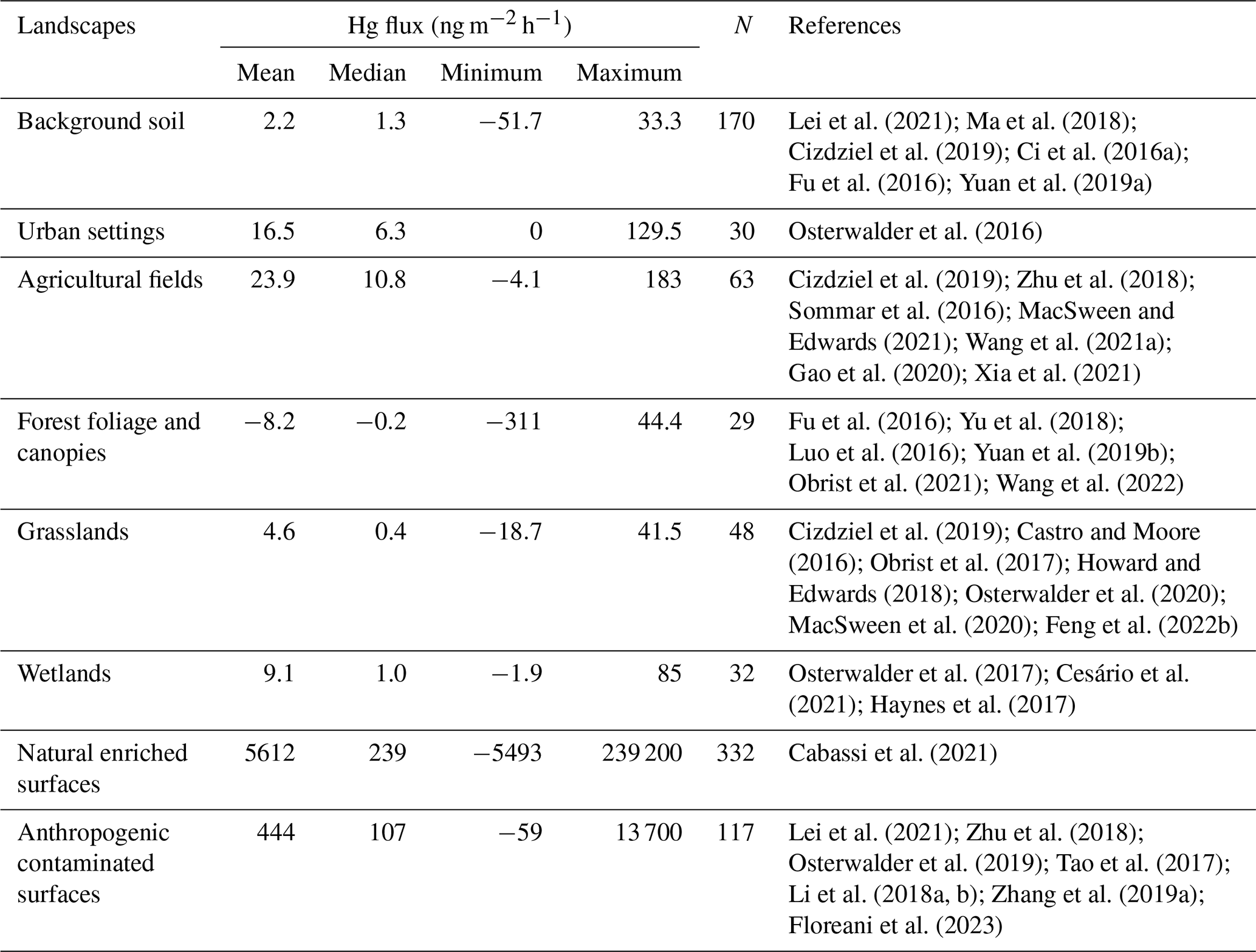
Currently, no long-term station measurements of Hg(0) fluxes from various terrestrial surfaces are available to evaluate modeled temporal trends; these are needed to improve the air–land Hg exchange budget estimates and to understand the kinetics of Hg(II)–Hg(0) redox chemistry and microbial processes in soils, particularly in areas of global land use changes due to climate change and human activities. We recommend creating and maintaining an updated database of air–vegetation–soil Hg exchange measurements, specifically network-based measurements using standardized methods, to understand the long-term trends and associated drivers. Since air–land Hg(0) exchange is bidirectional, flux measurement data cannot decouple the contributions of the deposition and evasion processes. Stable Hg isotope techniques are capable of quantifying the contributions of individual biogeochemical processes during air–soil Hg(0) exchange (Yuan et al., 2019a, 2023); their application is recommended to quantify the deposition and re-emission of Hg(0) in terrestrial ecosystems.
4.3 Ocean concentrations
The ocean links atmospheric concentrations to those of the food web. Currently, there is no systematic monitoring of marine Hg water concentrations, but an increasing number of cruise data are being published. This provides a possibility for the development of an observationally based picture of the large-scale spatial Hg variability. Ocean Hg models are important for filling the gaps in our knowledge of Hg spatiotemporal trends. However, to create reliable models, all available observational data should be used for model evaluation. There is therefore a need for development of a seawater Hg database (UNEP, 2022a – UNEP/MC/COP.4/INF/25), including data from as many expeditions as possible. Synthesizing the ocean concentration data would help describe spatial trends and play an important part in biogeochemical model evaluation.
A range of studies have presented observation-based basin and global ocean Hg concentration estimates for total or speciated Hg concentrations (e.g., Mason et al., 2012; Lamborg et al., 2014; Soerensen et al., 2016a), but Bowman et al. (2020) do so based on the largest number of observations (over 200 high-resolution, full-depth profiles of speciated Hg). The authors take advantage of recent global-scale oceanographic survey programs (CLIVAR and GEOTRACERS) focusing on offshore waters. Still, a large fraction of the data is collected outside of these two programs, many of these in pollution-impacted regions like downwind of Asia (Yang et al., 2017; Marumoto et al., 2018; Liu et al., 2020). A large subset of existing sample locations is indicated in Fig. 7 to give an idea of the global geographical extent of current ocean Hg observations.
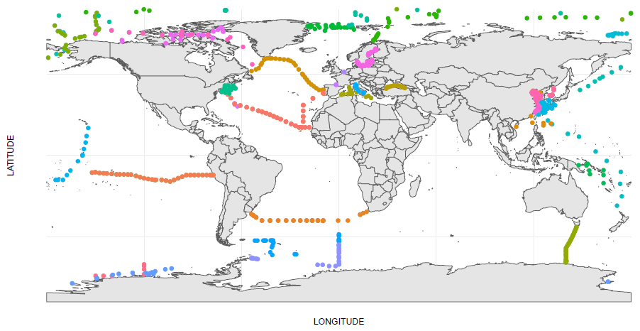
Figure 7THg and MeHg marine sampling locations shown with rosettes during the past ∼15 years and showing a global coverage (except for the Indian Ocean and parts of the Pacific Ocean). Note that this is a subset of existing published datasets. References: Agather et al. (2019), Bowman et al. (2015, 2016), Bratkič et al. (2016), Ci et al. (2016b), Cossa et al. (2018), Hammerschmidt et al. (2013), Jonsson et al. (2022), Kim et al. (2017, 2020), Marumoto et al. (2018), Munson et al. (2015), Nerentorp Mastromonaco et al. (2017a, b), Perrot et al. (2023), Petrova et al. (2020), Sharif et al. (2014), Soerensen et al. (2013, 2016a, 2018), Yang et al. (2017), Yue et al. (2023), and Wang et al. (2016a, 2020a). GEOTRACES cruises downloaded from the repository at https://www.bodc.ac.uk (last access: 1 May 2025).
A simple database in SQL, R, or another appropriate tool is recommended for creation based on the extraction of cruise information (period 2007–2022) from a few large data storage facilities (GEOTRACERS portal, BCO-DMO, PANGAEA, and BODC) and integration of other publicly available datasets (e.g., available in the supporting information of published papers). Furthermore, authors who have not yet made their datasets publicly available may be contacted to augment the ocean Hg observation coverage. The database will facilitate the analysis of observational patterns of oceanic Hg and MCHgMAP model evaluation.
For analysis of observational patterns, we suggest building on the methodology of Bowman et al. (2020) but with an extended number of observations. For MCHgMAP, a software package will be developed (1) to perform simple data analyses with a focus on investigating spatial trends by aggregating and computing standard statistics on data within user-defined time frames, depths, and areas (e.g., based on FOA major fishing areas; Table C2), similar to the model receptor regions (Sect. 6.2) or other divisions like ocean basin, provinces, and coastal boundaries (https://www.marineregions.org/sources.php, last access: 1 May 2025); and (2) to create an observationally based global mass budget for speciated Hg in the ocean.
The major limitation of ocean Hg observations is linked to the estimation of temporal trends, which is currently not feasible, neither in the long term (pre-2005) nor for the past decade. The lack of long-term stations measuring Hg in the ocean means that we must rely on sporadic cruises (different times of year and different ship tracks). Furthermore, for deeper offshore water, the ocean response time can be decades to centuries (Amos et al., 2013), while the variability in Hg observations for coastal and surface water is likely to be higher than anthropogenically driven decadal trends due to the sporadic observational coverage. There is also uncertainty related to observations performed prior to the introduction of clean measurement techniques, which were established in the 1980s but not used uniformly until later (Gill and Fitzgerald, 1987; Soerensen et al., 2012). This makes it difficult to know whether or how to include older observations (which could otherwise help explore multidecadal temporal trends).
To inform future EE efforts of Hg MEAs, the proposed database may be developed further by creating a formal network as suggested in UNEP (2021; UNEP/MC/COP.4/INF/12) and by creating an official way of submitting new data to the database.
4.4 Air–sea flux exchange
The ocean can exchange Hg with the atmosphere via diffusion of Hg(0) providing a sink for Hg in the ocean and prolonging the active cycling of Hg in the environment (Mason et al., 2017; Amos et al., 2013). There is currently no systematic monitoring of Hg fluxes and only a single study (Osterwalder et al., 2021) has measured the Hg(0) air–sea exchange flux directly with the use of micrometeorological methods in a coastal area. In all other cases, the Hg(0) flux is estimated through the use of thin film gas exchange models such as Liss and Merlivat (1986) and Wanninkhof (1992). These models use in situ measurements of Hg(0) in surface water and air together with wind-speed-dependent parameterization of the gas transfer velocity to calculate a flux. Flux estimation using the gas exchange model is dependent on especially Hg(0) measurements in surface water (Hg(0) in the atmosphere is less variable and therefore not as important in the calculation). However, while past evasion estimates were based on few Hg(0) observations collected on research cruises, in the last 2 decades, the amount of information has increased dramatically through the use of underway continuous sampling systems and the involvement in the GEOTRACES program (e.g., Andersson et al., 2008b; Mason et al., 2017; DiMento et al., 2019). The Hg air–sea exchange data (i.e., Hg(0) concentrations) from previous published papers (examples from recent years are Yue et al., 2022; Kuss et al., 2011; Soerensen et al., 2014; DiMento et al., 2019; Marumoto et al., 2018) cover nearly all oceans but on different timescales. These datasets have not been systematically stored anywhere, and there is therefore a need to develop a database including all information needed to calculate air–sea exchange based on gas exchange models. Synthesizing the Hg(0) ocean concentration data and auxiliary variables will help describe spatial trends and play an important part in the biogeochemical model evaluation.
While the major Hg species degassing from the surface ocean to the atmosphere is Hg(0) as described above, the current understanding is that both MMHg and DMHg can also evade from the surface ocean as a gas or within sea spray (Hammerschmidt et al., 2007; Weiss-Penzias et al., 2016). While such a flux can be important for distributing MeHg from the ocean to land, this flux is considered to be much smaller than that of Hg(0), and estimates are still so few that it may not be possible to include consideration of this flux at this time.
For the current multimodel study, we propose including observations relevant to calculating air–sea exchange (i.e., Hg(0) concentrations in surface air and water and associated environmental variables such as wind speed, air and water temperature, UV radiation, ozone, and other gas concentrations) in a format similar to that of the Hg Ocean Observational Database described in Sect. 4.3. In cases where raw data do not exist or are not available, the database could keep the averaged or ranged data for future reference. This would provide a way of reviewing spatial and temporal trends in the context of Hg biogeochemical cycling. The compiled data could be used to (1) create the best possible observationally based map that spatially resolves air–sea exchange on a global scale, (2) evaluate ocean models (see Sect. 6.2), and (3) create an observationally based global flux budget for Hg(0) across the air–sea interface (using the harmonized air–sea exchange formulation for the MCHgMAP described in Appendix B).
Currently, the patchiness of observations (geographical and temporal) in coastal and remote regions is a significant limitation. Furthermore, there are still a limited number of research groups that make high-resolution surface water Hg(0) measurements, and intercomparison between continuous analyzers and batch sample analyses are generally missing. To inform the future EE efforts of Hg MEAs, repeated observations of Hg(0) at one or more ocean locations to better evaluate seasonal and annual trends are needed. Opportunities for such an endeavor could be deployments of continuous dissolved gaseous mercury analyzers on cruises at stations where routine repeat cruises occur, e.g., BATS (Bermuda Atlantic Time Series) or HOTS (Hawaii Ocean Time Series) cruises, or on ferries or other vessels (research ships, as done for CO2) that cover a specific path routinely or are at sea continuously. The use of micrometeorological methods for ocean studies (Osterwalder et al., 2021) as well as observational and modeling studies on the Hg isotopes (Jiskra et al., 2021; Song et al., 2022) can provide additional approaches to constrain the Hg(0) evasion flux. For recommendations on the Hg Ocean Observational Database, see Sect. 4.3.
4.5 Environmental archives
One challenge in assessing the effectiveness of Hg MEAs is the lack of well-defined pre-impact and preindustrial baselines for Hg in the environment. Anthropogenic activities have caused the release of significant quantities of Hg to the air, water, and soil, beginning around 1550 (Streets et al., 2017, 2019a). To determine a true pre-impact baseline, long-term temporal records of Hg that date back not only to preindustrial times (pre-1850) but also pre-1550 are needed. Direct measurement of atmospheric Hg can be logistically challenging, particularly in remote locations, and it has only been possible since the 1990s. Very few monitoring stations exist around the world, and therefore the instrumental record is temporally and spatially limited. In the absence of direct long-term Hg measurements in the environment, natural archives such as peat bogs (Bindler, 2003; Enrico et al., 2017), lake sediments (Engstrom et al., 2014; Muir et al., 2009), ice cores (Beal et al., 2015), and tree rings (Clackett et al., 2018; Ghotra et al., 2020) provide a means of reconstructing long-term trends in atmospheric Hg concentration and deposition, and hence they provide valuable information on long-term changes in anthropogenic Hg emissions and their environmental cycling via re-emission and soil mobilization. Thus, natural archives provide important constraints for developing and evaluating Hg models (especially mass balance models). Mass balance models, in turn, provide an understanding of the lifetime of Hg in various environmental matrices, which is important for MC. Natural archives show an increase in the Hg deposition in remote locations by a factor of 3–5 since the industrial revolution (1850) and the peak in the 1970s, followed by 2-fold decline but also a lack of decline in some remote lake sediment archives, likely due to continued mobilization of legacy Hg from watershed soils (Sonke et al., 2023; Zhang et al., 2014b; UNEP, 2019; Li et al., 2020a; Faïn et al., 2009; Enrico et al., 2017).
Lake sediment records are produced by the annual sinking of particulate-bound Hg to lake bottoms and reflect Hg that has entered lakes both directly via atmospheric deposition as well as from catchment contributions. Lake sediment records have proven to be reliable for reconstructing historical trends in the total deposition of Hg. For example, sediment-derived Hg deposition estimates have been shown to compare well to those obtained from wet precipitation instruments for modern times (Wiklund et al., 2017; Roberts et al., 2019, 2021), to compare well to those derived from the GEM-MACH-Hg model (Muir et al., 2009; Roberts et al., 2021), and to reliably track changes in reported Hg emissions from various industrial operations, such as smelters, Hg and gold mines, and chlor-alkali plants (Lockhart et al., 2000; Wiklund et al., 2017; Roberts et al., 2019). Unlike lake sediments, ice caps and glaciers receive Hg inputs solely from atmospheric sources and thus can be useful for reconstructing temporal trends in atmospheric Hg deposition. Because ice mass accumulation rates are known to impact rates of Hg deposition and accumulation, either by increasing Hg deposition or the efficiency with which this Hg is buried and accumulated (as opposed to being remitted into the atmosphere following photoreduction), ice core records are more useful for reconstructing temporal trends in atmospheric deposition than determining flux magnitude (Lemire, 2021). Similar to ice cores, tree rings can be used to determine the pre-anthropogenic impact baseline for Hg in the environment as tree ring chronologies can extend back 1000 years or more (Clackett et al., 2018; Ghotra et al., 2020). Tree rings have the distinct advantage of being resolved annually and dated to the calendar year using standard dendrochronology methods (Bridge, 2001) and are not subject to high radiometric dating uncertainties and low temporal resolution, which commonly apply to sedimentary archives. Both experimental and field data suggest that trees actively assimilate mainly Hg(0) species from the atmosphere via stomatal uptake, followed by translocation through the phloem and accumulation in annual growth rings (Peckham et al., 2019a; Arnold et al., 2018; Stamenkovic and Gustin, 2009; Laacouri et al., 2013; Maillard et al., 2016; Zhang et al., 1995; Siwik et al., 2010; Odabasi et al., 2016; Navrátil et al., 2019; Jung and Ahn, 2017; Hojdová et al., 2011; Becnel et al., 2004; McLagan et al., 2022). Thus, tree rings can serve as biomonitors for atmospheric Hg(0).
There are numerous published Hg sediment records spanning the past 100–200 years due to the ease of collecting “short cores” using gravity corers and the availability of 210Pb dating to derive ages and sediment accumulation rates (g m−2 yr−1) with 137Cs dating often also used as an independent tracer to validate the 210Pb chronology (Blais et al., 1995). Cores which span the pre- and post-industrial periods (pre- and post-1850) enable levels of post-industrialization anthropogenic Hg enrichment and depositional fluxes (µg m−2 yr−1) to be calculated. The comparison between sediment-derived Hg fluxes from multiple lakes/locations is commonly conducted by applying a sediment focusing factor based on a comparison of 210Pb fluxes in lake sediment and catchment soils, which accounts for in-lake sedimentation processes (Blais et al., 1995; Perry et al., 2005; Muir et al., 2009). Anthropogenic versus geogenic origin of Hg in lake sediments can be isolated by applying geochemical normalization to Hg concentration data given a strong correlation between Hg and lithogenic elements such as aluminum (Al), lithium (Li) and titanium (Ti) (Loring, 1991; Kersten and Smedes, 2002; Wiklund et al., 2017; Roberts et al., 2019). Furthermore, catchment Hg runoff to lakes can also be subtracted from the sedimentary record using a “catchment effect” correction when sedimentary Hg accumulation and the catchment area to lake area ratio are linearly correlated, allowing a reconstruction of atmospheric deposition (Drevnick et al., 2012; Wiklund et al., 2017; Roberts et al., 2019). There are several recent papers that summarize spatial and temporal trends Hg fluxes over large geographical areas using 30–138 lake sediment cores; however, deposition Hg fluxes in these papers have been corrected to varying degrees (Drevnick et al., 2016; Muir et al., 2009; Kirk et al., 2011; Roberts et al., 2021). Longer term records covering the preindustrial period are less common as they often require longer cores collected using a percussion corer and a combination of 210Pb and 14C dating methods; however, depositional Hg fluxes spanning the last 500–2000 years are available from cores collected in remote regions of North America, South America, and an equatorial crater lake from Mount Kilimanjaro, Africa (Engstrom et al., 2014; Biester et al., 2018).
Ice core dates, an age–depth scale, and ice mass accumulation rates are derived from δ18O record and ion chemistry analyzed over the length of the core. There are several Hg deposition records inferred from ice and firn cores from the Arctic (Greenland; Ellesmere Island including Mount Oxford, Agassiz ice cap, and Prince of Wales ice field; Devon Island: Devon ice cap; Baffin Island: Penny ice cap) and high-elevation, lower-latitude sites (Yukon: Mt. Logan; Wyoming: Upper Fremont Glacier; Central Asia: Belukha glacier) (Beal et al., 2015; Eyrikh et al., 2017; Zheng et al., 2014; Zheng, 2015; Schuster et al., 2002; Chellman et al., 2017; Zdanowicz et al., 2013, 2015, 2016, 2018; Lemire, 2021); however, few of these capture the preindustrial period (Beal et al., 2015; Eyrikh et al., 2017; Zheng, 2015; Jitaru et al., 2009).
The development of tree rings as a tool to monitor trends in atmospheric Hg is an area of active research. Therefore, tree ring records of Hg are still subject to a number of limitations. For example, tree ring Hg measurements provide information on the relative change in atmospheric Hg(0) over time but cannot be converted into absolute concentrations in air, at least not until a number of tree ring records are calibrated against co-located direct measurements of Hg(0) in air. Because of the mechanism of Hg(0) uptake from air into plants via stomata, tree ring Hg concentrations reflect growing season atmospheric Hg(0) concentrations and not annual mean Hg(0) concentrations. To date, the ability of tree rings to faithfully record atmospheric mercury has only been investigated in a small number of species, and some of those species have been shown to be inadequate biomonitors due to translocation, causing a shift in the temporal dendro-chemical record (Nováková et al., 2021; Wang et al., 2021c). The applicability of tree ring Hg records to spatial coverage might be limited due to the geographical range of suitable tree species, similarly to how ice core records of Hg deposition and accumulation are limited to high-latitude or high-elevation sites.
To inform the MCHgMAP multimodel study, temporal trends of Hg concentrations and depositional flux magnitude derived from sediment cores, ice cores, and tree ring records for both the preindustrial and postindustrial periods will be compiled and compared to constrain Hg mass balance modeling. Both total or uncorrected and fully corrected (for sediment focusing and catchment contributions) sediment-derived Hg fluxes may be compiled, with the latter likely better reflecting wet plus dry atmospheric contributions.
Since lakes and forested areas are widely distributed around the world, sediment core and tree ring Hg data allow for the potential development of a global network of multi-century Hg time series (Eccles et al., 2020) to evaluate global atmospheric Hg emissions as well as the spatial footprint and environmental impact of local Hg(0) emissions from point sources (Clackett et al., 2021; Navrátil et al., 2017, 2018; Perone et al., 2018; Schneider et al., 2019; McLagan et al., 2022). Because temporal changes in atmospheric Hg(0) concentrations are not globally synchronous (Dastoor et al., 2015; Steffen et al., 2015), sediment cores and tree ring records collected from different geographic locations can elucidate the spatial variability of these trends. A globally distributed network of sediment-derived fluxes, including a subset of long cores spanning the era before 1550 and corrected for sediment focusing and catchment or geogenic Hg inputs, could be particularly useful for quantifying both baseline changes and changes in Hg deposition over time. Ice core data are useful for assessing changes in Hg deposition in high-elevation, high-latitude locations, and efforts should be made to collect these data prior to further degradation of the Hg deposition record due to climate-change-driven melting of glacial ice. Furthermore, records of Hg concentrations and deposition across time and space should be leveraged further and used to assist in the validation of mechanistic process-driven mercury models. Finally, the quantification of Hg stable isotope ratios in sediment, cores, and tree rings holds promise for source attribution, including resolving Hg local industrial sources from regional or global sources (Lee et al., 2021; Sun et al., 2022; Lepak et al., 2020; Scanlon et al., 2020).
The available models and data described in the preceding sections can provide essential information on the MC and LRTAP EE efforts, addressing several of the guiding questions outlined in the MC monitoring guidelines (UNEP/MC/COP.4/INF/12; see Appendix A). Mechanistic models are essential tools for distinguishing the influences of temporal trends in emissions and releases from other environmental drivers on observed trends in Hg levels in the air, biota, and humans. This section describes the MCHgMAP experimental design for a coordinated set of multimedia, multimodel ensemble simulations between atmospheric, oceanic, and mass balance models to develop EE-relevant insights into global and regional Hg cycling.
Terrestrial ecosystems play a major role in retaining and mobilizing deposited Hg across the air–land–ocean interface; thus, accounting for the variations in terrestrial Hg occurring due to changes in anthropogenic emissions is important for global Hg cycling. Additionally, alterations of land cover, biogeochemical and hydrological characteristics, and meteorological conditions (driven by climate change and other anthropogenic influences) influence net terrestrial exchange of Hg with the atmosphere and downstream aquatic systems. Schaefer et al. (2020) estimated that thawing circumpolar Arctic permafrost regions can lead to Hg re-emissions comparable to the current global anthropogenic emissions by 2200 in a high-emission climate scenario. As noted in Sect. 2, spatially explicit air–terrestrial–hydrological modeling presently remains a major research challenge, largely due to the biogeochemical heterogeneity and complexity of terrestrial ecosystems (Bishop et al., 2020). The influences of changes in meteorology (such as temperature, precipitation, soil moisture, and snow cover), primary productivity, and wildfires will be modeled in this work via surface–atmosphere parameterizations in atmospheric models using inputs from weather models and satellite-based products. Also, the changes in terrestrial legacy Hg emissions and releases driven by long-term changes in anthropogenic emissions are considered based on multimedia mass balance modeling. However, other important global change impacts such as those related to permafrost thaw and hydrological modifications are not incorporated into the first set of model simulations. Model scenarios to further investigate the effects of global change on environmental Hg levels will be developed in future scenarios in a later phase of the project utilizing current advances in terrestrial Hg.
Three-dimensional atmospheric and oceanic models require geospatially and chemically distributed time series of emissions to drive and observational data to evaluate the models. Preparation of global anthropogenic Hg emission inventories is a complex exercise (see Sect. 3.2), and the methods have been updated continuously since the development of an initial inventory for 1990 (AMAP/UNEP, 2008). Currently, most up-to-date global anthropogenic Hg emission inventories are available starting ca. 2010 (e.g., UNEP, 2019; Streets et al., 2019b). The global anthropogenic Hg emission inventories are planned for extension to 2020 to facilitate the effectiveness evaluation of the MC (see Sect. 3.2.1). In addition, development of future scenarios of Hg emissions up to 2050 spanning policy-relevant conditions such as no additional control, an MC Hg control policy, co-benefits from other air pollutants' abatement, and a range of climate scenarios is planned (see Sect. 3.2.2). Regarding Hg observations for the MME evaluation, a literature survey of Hg observations from various environmental compartments suggests more comprehensive coverage in the last decade; these datasets will be prepared in collaboration with other ongoing efforts to support the MC EE (see Sect. 4).
Since anthropogenic emission inventories and observations are best defined starting around 2010, detailed 3D atmospheric and oceanic multimodel simulations are proposed for the years 2010–2020 to analyze the spatial patterns and temporal trends of Hg levels from the period beginning prior to the MC (ca. 2010) and extending as close as possible to the present (referred to as “recent levels and trends”). Future projections of Hg levels in the air and ocean from 2020 to 2050 will be simulated using the proposed set of future Hg emission scenarios (see Sect. 3.2.2). In addition to 3D modeling of recent historic and near-future Hg levels, examination of the long-term changes in Earth's biogeochemical cycling of Hg from the pre-anthropogenic period to the present and future is proposed using multimedia mass balance model simulations. Mass balance models are driven by all-time changes in geographically aggregated primary emissions and releases of Hg estimated from information on historic anthropogenic activities (Guerrero and Schneider, 2023; Streets et al., 2019a; Amos et al., 2015), and they are evaluated against Hg levels from natural environmental Hg archives (see Sect. 4.5).
5.1 MCHgMAP simulation approach
Several Hg multimodel ensemble intercomparison studies have been carried out during the past decade on global (AMAP/UNEP, 2013; UNEP, 2019; Travnikov et al., 2017; Bieser et al., 2017) and regional (Angot et al., 2016; Dastoor et al., 2022a, b; Gencarelli et al., 2017) scales. These multimodel studies have mainly focused on the assessment of atmospheric Hg, its spatial distribution, source–receptor relationships, chemical mechanisms, and other processes. The model simulations in these multimodel studies lacked full accounting of changes in secondary Hg emissions from the land and ocean, limiting their utility in analyzing temporal trends of Hg in the environment. In MCHgMAP, we expand the multimodel Hg assessment to global oceans and propose a harmonized MME simulation approach between 3D mechanistic atmospheric and marine models, multimedia mass balance models, and mechanistic air–land exchange models to account for the short- and long-term influences of changes in primary anthropogenic Hg sources and environmental conditions on Hg cycling between land, atmosphere, and ocean.
The harmonized modeling approach is designed to simulate the evolution of primary and secondary sources of Hg emissions and releases to the air and ocean: (1) to generate spatially resolved maps of recent Hg levels (concentrations and fluxes), filling monitoring gaps; (2) to detect their spatial gradients and temporal trends; (3) to attribute the levels and trends to emission sources and environmental drivers; (4) to quantify the impacts of MC and LRTAP implementations on Hg levels and trends; (5) to quantify the uncertainty and sensitivity of modeled Hg levels and trends; (6) to develop insights into future Hg cycling under different scenarios of implementation of the Minamata Convention and other MEAs and changing environmental conditions across global regions; and (7) to improve the understanding of environmental Hg processes and their parameterizations in models. The simulations address the MC and LRTAP EE policy questions listed in Appendix A.
To accomplish the above objectives, we broadly define three types of model simulations:
-
Baseline simulation. A state-of-the-art simulation of Hg levels and trends over the historical or future period, capturing the range of variability between models.
-
Perturbation simulations. A simulation either zeroing out a model driver, fixing a model driver to a certain year's values, or fixing all drivers but one to a certain year's values, conducted to diagnose the contribution of the driver to Hg levels or temporal trends.
-
Sensitivity simulations. A simulation using a modified driver dataset or parameterization, conducted to probe the sensitivity of model results to that driver or process.
Additional details of the simulation design are provided in the next two sections. Below we describe the proposed approach for the coordination of MME simulations between atmospheric, oceanic, and mass balance models in the context of analyzing recent Hg levels and trends. Coupled atmosphere–ocean simulations for future scenarios will be performed using a strategy analogous to that used to conduct the simulations for the recent Hg trends. Close collaboration to equilibrate the ensemble of atmospheric and oceanic models is proposed during the baseline and perturbation simulations (Tables F8–F10), which is important for producing consistent estimates of Hg levels and fluxes between the atmosphere and oceans. This approach consists of the following four stages, as illustrated in Fig. 8:
-
Stage 1: initialization of atmospheric and oceanic models with harmonized drivers. The atmospheric modeling groups will conduct 2015 simulations with the updated set of harmonized model drivers (Table F5) and the Hg(0) sea surface concentration dataset from Horowitz et al. (2017). Ensemble monthly mean deposition and concentration data for the year 2015 from the atmospheric models will be transferred to ocean modeling groups. Ocean models will use the 2015 Hg(II) deposition and Hg(0) air concentration fields as inputs for a spinup simulation long enough to equilibrate Hg concentrations in the ocean adopting drivers proposed in Table F6.
-
Stage 2: baseline simulations in atmospheric and oceanic models. For consistent baseline simulations between atmospheric and oceanic models to reproduce environmental Hg levels, we will follow an iterative procedure, previously used to couple MITgcm and GEOS-Chem (Horowitz et al., 2017). Simulations for the period 2010–2020 will be initiated in atmospheric models, using the Hg(0) sea surface concentration dataset from Horowitz et al. (2017). Hg(II) deposition and Hg(0) air concentration fields from the individual atmospheric models will be averaged into ensemble monthly means. The 2010–2020 ensemble mean atmospheric fields will be passed to oceanic Hg models, to be used as inputs for their 2010–2020 simulations. Sea surface concentrations of Hg(0) from the oceanic models will be averaged into ensemble monthly means for 2010–2020, which can then be provided back to the atmospheric models for input into their simulations. We will conduct two to three iterations of this approach to reach convergence of the ensemble mean of atmospheric and oceanic baseline model simulations. This procedure will produce 2010–2020 ensemble mean sea surface Hg(0) concentrations (which will be the standard inputs for further atmospheric simulations) and ensemble mean deposition and Hg(0) air concentration fields (which will be the standard inputs for further oceanic simulations).
-
Stage 3a: mass balance simulations with updated rate constants. Mass balance models require globally averaged estimates of rate constants for processes that transfer Hg between different environmental compartments (see Table F7). The ensemble mean data for the atmospheric and oceanic baseline simulations (2010–2020) will be used to calculate updated rate constants needed for the mass balance simulations. Rate constants for terrestrial pools will be estimated based on the past literature (Amos et al., 2013, 2015; Qureshi et al., 2011). In doing so, we will update the GBC box models to be consistent with the state-of-the-art 3D atmospheric and oceanic models for the purposes of this study. Uncertainty bounds for the rate constants will also be estimated from the variability of individual atmospheric and oceanic models within the ensemble, for use in sensitivity simulations of the mass balance model. The legacy re-emission trend and magnitude predicted by the GBC box model can be used as input for further sensitivity simulations in the 3D atmospheric and oceanic models.
-
Stage 3b: perturbation simulations in atmospheric and oceanic models. Atmospheric models will run perturbation simulations for 2010–2020 (Table F8), e.g., turning off all anthropogenic Hg emissions. The individual atmospheric models' deposition and concentration fields will be averaged into ensemble monthly mean fields. The atmospheric ensemble mean fields will be passed on to the oceanic models as inputs for their perturbation simulations. As opposed to Stage 2, a selection of perturbation experiments will be considered for multiple iterative rounds of simulations for the atmosphere–ocean coupling, depending on the computational expense and time constraints. For example, a coupled atmosphere–ocean “nature simulation” for 2010–2020, where primary anthropogenic emissions are kept fixed at the 2010 level and the Hg trend is solely driven by natural factors, will be performed using the iterative approach.
-
Stage 4: further sensitivity analysis in models. Atmospheric, oceanic, and mass balance models will conduct further sensitivity simulations, e.g., testing the uncertainty of model simulations to different driver datasets, conducting idealized emission trend experiments, and testing the uncertainty in different model parameterizations (e.g., air–sea exchange parameterizations) and input fields (e.g., Hg and MeHg loads from rivers in the ocean models). During this phase, atmospheric and oceanic models do not require coupling for their individual experiments.
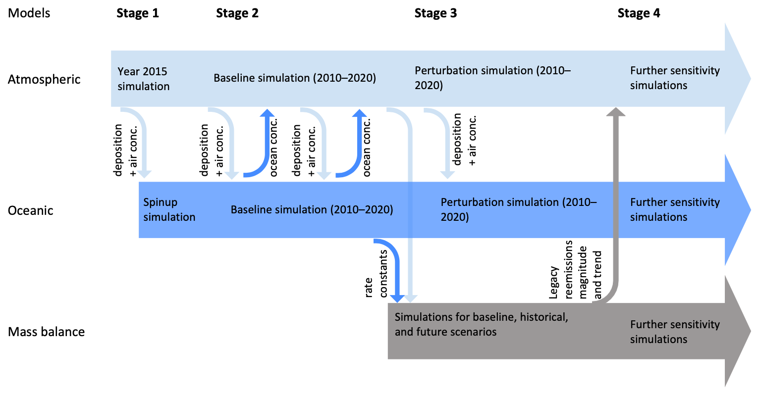
Figure 8Diagram showing how the coupling between the atmospheric, oceanic, and mass balance models will be achieved by conducting the work in stages and exchanging information between the model types in MCHgMAP.
5.2 Three-dimensional atmosphere and ocean simulations
The proposed coordinated multimodel atmospheric and oceanic model simulations for MCHgMAP are presented in Tables F8 and F9. Most of the model simulations will be performed for the period 2010–2020 for historical trends and from 2020 to 2050 for the future scenarios, except for several optional sensitivity simulations, which can be conducted for individual years. Appropriate model spinup to reach steady-state conditions is required; a consecutive simulation from 1980 to 2020 starting from semi-realistic initial conditions is recommended for ocean models, while a spinup of approximately 5 years is needed for atmospheric models. The primary and secondary emissions for atmospheric models over land are provided by emission inventories and mechanistic air–land Hg exchange model simulations (Sect. 3), and over oceans the boundary conditions are exchanged between atmospheric and ocean models, as described in the previous section (Fig. 8). The model simulations in Tables F8 and F9 are divided into five groups, in accordance with their purposes:
- i.
The “baseline” simulation (A1; O1) aims to obtain global patterns and temporal trends of atmospheric and oceanic Hg concentrations and fluxes utilizing state-of-the-art model configurations for model evaluation (Sect. 6) and analysis (Sects. 7 and 8) of observed Hg levels based on the modeling. The simulation will be performed using temporally varying default set of drivers (marked in bold in Tables F5 and F6) that are harmonized as much as possible between the models (using a combination of updated harmonized and model-specific input datasets and parameterizations).
- ii.
The “Source contributions” group (A2.1–A2.6; O2.1–O2.6) is focused on assessment of the relative contributions of various primary and secondary emissions and releases from anthropogenic and natural sources to Hg levels in the air and ocean. It consists of perturbation simulations with zeroed emissions from specific source types.
- iii.
The “Trend analysis” group (A3a.1–A3c.12; O3.1–O3.14) is intended to evaluate contributions of various anthropogenic and environmental drivers to recent changes in Hg levels over the considered period (2010–2020). This group is divided into three subgroups: “Contributions of various drivers to trends” (A3a.1–A3a.4), “Effects of changes in various drivers on trends” (A3b.1–A3b.7), and “Contributions of HTAP region anthropogenic emission changes to trends” (A3c.1–A3c.12). HTAP regions are the geographical world regions used in previous modeling experiments organized by the LRTAP Task Force on Hemispheric Transport of Air Pollution (Galmarini et al., 2017). These regions are defined in Appendix C. The perturbation simulations in the first and third subgroups are carried out with one driver fixed at the values corresponding to 2010 for the whole period, with other drivers varying in accordance with the baseline simulation. The perturbation simulations in the second subgroup are carried out with one driver varying as in the baseline simulation and all of the other drivers fixed at values corresponding to 2010. The comparison of the perturbation simulations with the results of the baseline simulation provides contributions to or effects on the considered drivers of the trend in Hg levels.
- iv.
The “Sensitivity analysis” group (A4.1–A5.10; O4.1–O4.7) is divided into two subgroups: “Uncertainty experiments” (A4.1–A4.8) and “Idealized experiments” (A5.1–A5.10). The first subgroup of simulations diagnoses modeling uncertainties using alternative driver datasets when available (e.g., multiple anthropogenic emission inventories may be available for the time period 2010–2020) or alternative parameterizations (e.g., multiple air–sea exchange parameterizations could be compatible with available measurements). In the “Idealized experiments” subgroup, sensitivity of Hg levels and trends to a driver or parameterization is assessed by replacing it with a hypothetical option. For example, to test the importance of accurate speciation in emission inventories, an extreme scenario could be simulated where all anthropogenic Hg is emitted as Hg(0).
- v.
The “Future scenarios” group (A6.1–A6.3, O5.1–O5.3) estimates future changes of Hg levels over the considered period (2020–2050) using available scenarios of anthropogenic emissions and projected environmental conditions and ascribes the estimated changes to various anthropogenic and environmental drivers.
Changes in primary anthropogenic emissions and releases and environmental conditions (physical and biochemical) form the two groups of forcings (or drivers) responsible for changes or trends in environmental Hg levels through their influences on Hg processes (i.e., Hg transport, biochemistry, and flux exchanges). In the proposed experimental design, the contributions of these two groups of drivers are first separated via the “nature simulation” (using coupled A3a.1 and O3.1), where primary anthropogenic emissions are kept fixed at the 2010 level and the Hg trend is solely driven by natural factors. The anthropogenic contribution is then further divided between contributions of ASGM (A3a.2), Minamata Annex D (A3a.3), and other sources. It is important to note that the contribution of changes in anthropogenic emissions is itself modified by the concurrently occurring environmental changes, which is reflected in these estimates. Isolating individual contributions of changes in various environmental conditions (such as meteorological, land, and ocean parameters) is difficult due to their interdependencies. Nonetheless, the individual effects of changes in a suite of environmental drivers on Hg levels can be examined by selectively allowing temporal variations of these drivers or their impacted Hg processes (e.g., Hg transport and secondary emissions and releases), while keeping all other drivers fixed in perturbation experiments (A3b.1–A3b.7). In addition, proposed idealized experiments (A5.1–A5.10), despite their simplicity, can reveal fundamental response characteristics of the model drivers or parameterizations and inform their potential impacts on future Hg cycling.
Tables F8 and F9 represent an extensive list of potential simulations, yet one must account for time and resource restrictions of participating models. Therefore, the model experiments are ranked in three priority levels (Tables F8 and F9): (1) “Core simulations”, expected to be performed by all global models; (2) “Optional simulations”, expected to be performed by as many models as possible; and (3) “Future simulations”, expected to be conducted as a third set of model simulations following the modeling and analysis of historical Hg levels. Both global and regional models can take part in the simulation program. The time-variable boundary conditions for regional modeling experiments will first be extracted and stored from multimodel simulations of global models. The model output variables (Tables F11 and F12) will be stored in open-data format (netCDF) with appropriate metadata. This includes the definition of new official Climate and Forecast (CF) convention tags for marine Hg variables (Davis et al., 2020) (see Appendix D).
5.3 Multimedia mass balance simulations
Given the dominant role of secondary emissions in contemporary Hg levels, quantifying their changes is important for the attribution of observed temporal trends of Hg in recent decades and future projections of environmental Hg cycling. Currently, it is difficult to fully account for the temporal trend in secondary emissions and releases based on observations or 3D Hg models alone. Multimedia mass balance box models have been used to trace the movement of all-time anthropogenic mercury emissions and releases and their influence on Hg levels in environmental matrices (Amos et al., 2015).
Multimedia mass balance simulations (see Sect. 2.4) will serve three primary MCHgMAP objectives: (1) determination of the sensitivity of environmental Hg levels and trends to uncertainty in emission histories and lifetimes of global Hg cycling, (2) attribution of secondary Hg emissions and releases and environmental Hg levels and trends to all time anthropogenic Hg sources, and (3) response of global Hg cycling to future anthropogenic emission scenarios. Mass balance models serve an additional purpose for the coordinated MCHgMAP simulations, which is to provide the changes in secondary emissions and releases (i.e., legacy emissions and releases) and/or environmental levels driven by historic changes in anthropogenic Hg emissions and releases as inputs to 3D atmospheric and ocean models. Mass balance model simulations represent a global geographic domain and will generally be performed for a period of more than 500 model years (e.g., 1500–2020, baseline simulation). Simulations will produce annual arrays of multimedia reservoir Hg levels and fluxes that can be stored as tables for analysis.
To account for uncertainties of Hg in emissions, reservoirs, and inter-compartmental fluxes, a mass balance model ensemble will be produced (see Fig. 9). Sensitivity simulations can be evaluated against available independent constraints (see below) in a similar manner to Amos et al. (2015). The list of simulations to be performed with the model ensemble is given in Table F10. The legacy component of environmental Hg will be developed and evaluated following the methodology of Angot et al. (2018).
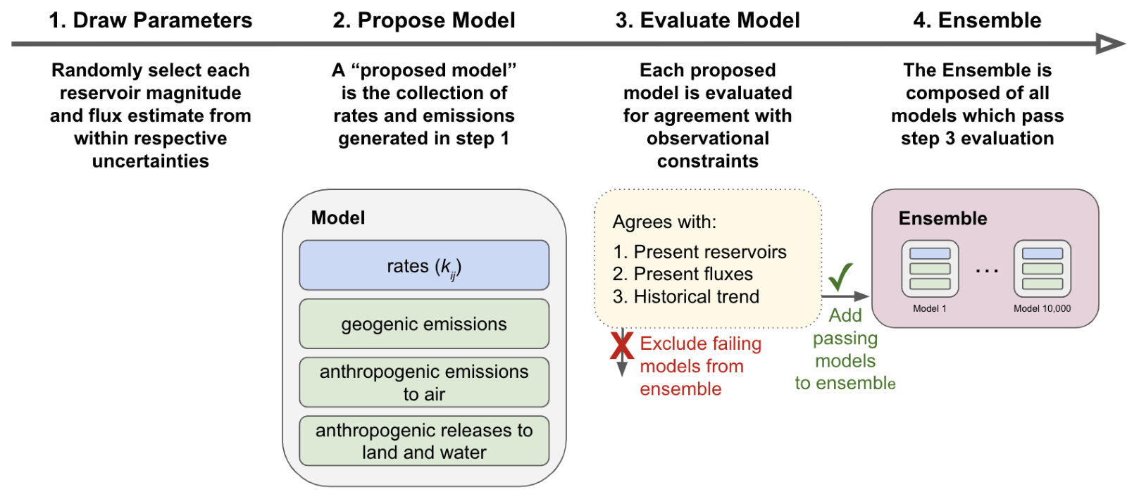
The plan for the construction of revised mass balance model ensemble (steps 1–4 below) and its simulations (steps 5–7 below; Table F10) is as follows:
- i.
Update rate coefficients: update central estimates for rate coefficients based on state-of-the-science review of contemporary Hg reservoir magnitude and exchange flux estimates (from models and observations). Rate coefficients used in baseline steady-state simulations from 3D air and ocean models will be considered.
- ii.
Develop the base model (steps involving model simulation): use a perturbational approach to define the set of rates and historical emissions and releases that are consistent with evaluation metrics (see below).
- iii.
Evaluate the model: the combination of feasible rate coefficients and emissions and releases trajectories will be constrained by model ability to reproduce:
- a.
Contemporary reservoir magnitudes (e.g., Sect. 4.1 and 4.3)
- b.
Contemporary fluxes (e.g., Sect. 4.2 and 4.4)
- c.
Historical trends in environmental archives (Sect. 4.5)
Model evaluation metrics should reflect global magnitudes/trends, which may require rescaling or re-balancing due to differences in regional sampling density of observations.
- a.
- iv.
Model ensemble: all box models (i.e., combinations of rate coefficients and emissions and releases trajectories) that successfully reproduce global magnitudes/trends (step 3) will compose the model ensemble (i.e., baseline simulation M1; Table F10) used in the following analysis simulations.
- v.
Characterize secondary emissions and release trends (steps involving model simulation): quantify contributions of legacy and recent primary emissions to recent temporal trend (i.e., 2010–2020) in global Hg levels and secondary emissions from the land and oceans (Simulations M2 to M11 in Table F10). Uncertainties in contributions will be bounded using the model ensemble.
- vi.
Perform attribution of temporal trends to primary sources (steps involving model simulation): quantify the fraction of all-time trend in global Hg levels and secondary emissions and releases attributable to specified primary source categories (Simulations M12 to M17 in Table F10).
- vii.
Project future effects of policy interventions (steps involving model simulation): quantify temporal trend in Hg levels and secondary emissions and releases under future anthropogenic emission scenarios (simulation M18 and M19 in Table F10).
Further development of spatially resolved mass balance models (e.g., hemispheric- or ocean-basin-resolved compartments) including Hg speciation would improve the analysis of all-time Hg trends. Importantly, accounting for changes in intermedia exchange rates due to changes in environmental conditions such as oxidant concentrations or precipitation regimes, or changes in terrestrial Hg export to coastal ocean due to accelerated permafrost thaw and erosion is needed to perform sensitivity simulations to quantify response of secondary emissions and releases and reservoir Hg burdens under future climate change scenarios.
Evaluation of the MME simulations against observational data is of key interest and relevance both scientifically and to the MC and LRTAP effectiveness evaluations. The primary goal of this model evaluation is to assess the robustness of baseline historical simulations to facilitate observationally constrained attribution of observed changes in global Hg levels to anthropogenic and natural forcings and to predict future Hg levels. The discrepancies between modeling and measured data indicate areas of increased uncertainty and provide directions for further improvement of the models, model inputs (e.g., emission data) or measurement data. Additionally, in the regions where measurements are absent or for the parameters and processes which are not directly measured, the intercomparison of results from different models can provide additional information on the level of uncertainties. To facilitate the intermodel comparison and the evaluation of the modeling results against observations, the spatially resolved variables from 3D models will be interpolated from the model-specific grids to a unified latitude–longitude grid and to the points of measurement sites' location, respectively. The evaluation of mass balance model historical simulations is discussed in the preceding section (Sect. 5.3). The following sections present the MME approach for the evaluation of recent Hg levels and trends simulated by the 3D atmosphere and ocean models.
6.1 Atmospheric models
Comparison of model simulations with measurement data is a standard evaluation procedure applied for various purposes – model development, integrated analysis and evaluation of modeling results, and process studies. A variety of single-model and multimodel studies have used measurements to support research of Hg dispersion on a global scale (Horowitz et al., 2017; Shah et al., 2021; Zhang and Zhang, 2022) or in the polar regions (Angot et al., 2016; Dastoor et al., 2022a, b) to evaluate emission inventories and their trends (De Simone et al., 2016, 2017a; Zhang et al., 2016b; Giang et al., 2018) and to study Hg chemical mechanisms (Shah et al., 2016; Song et al., 2018; Saiz-Lopez et al., 2018, 2020) and other processes in the atmosphere (Gencarelli et al., 2017; Travnikov et al., 2017; Bieser et al., 2017).
A variety of available measurement data will be used for evaluation of the multimodel atmospheric simulations, including ground-based measurements from global and regional networks, aircraft measurements, ship and terrestrial flux measurements. In addition, the simulated concentrations of Hg species, wet and dry deposition, air–surface exchange fluxes and relative contribution of various emission sources and sectors will be compared between models. Table F11 summarizes the output variables to be used in the model evaluation. Different characteristics of atmospheric Hg will be evaluated in both the model–measurement and model–model comparisons, as follows:
-
Spatial distributions (comparison with ground-based measurements): the comparison will include temporally averaged Hg levels, spatial correlation, and gradients. It is important to evaluate different measured parameters (e.g., Hg(0)/Hg(II) concentrations, Hg wet deposition). This comparison can evaluate the models' atmospheric chemistry and global mass balance of sources/sinks.
-
Temporal trends (comparison with ground-based measurements): the comparison will include temporal changes at individual sites or average values over different regions. It is important to combine different measured parameters (Hg(0) concentration, Hg wet deposition) since they characterize the relative contributions of global and regional sources. This comparison can provide evaluation of the modeled changes driven by emissions (anthropogenic and legacy) and effects of other drivers (e.g., meteorology, land cover, leaf area index LAI, and sea ice). In addition, the analysis of seasonal variations provides insights into major sources and sinks of atmospheric Hg.
-
Vertical profiles (comparison with aircraft measurements): the comparison will be focused on vertical distribution of Hg species (Hg(0), Hg(II)) at certain locations. The analysis provides additional insights into free tropospheric processes (Hg chemistry) and the effect of emission sources (e.g., power plants or volcanoes).
-
Air–surface exchange (comparison with ship and terrestrial flux measurements): this will consist of a comparison of Hg concentrations (Hg(0), Hg(II)) and estimated air–sea exchange fluxes at locations of ship measurements and comparison of Hg dry or throughfall deposition and exchange fluxes at terrestrial sites.
-
Spectral analysis (comparison with ground-based measurements, model intercomparison): in addition to the traditional model–measurement comparison using scatter plots and statistical metrics (e.g., bias and correlation, R2), spectral analysis will be used to examine and compare model and observed data (Sirois et al., 1995; Bowdalo et al., 2016). This will further help in determining which data characteristics (e.g., seasonal cycles or diurnal cycles) are best reproduced by the models.
The model evaluation is limited by the sparse geographical and temporal coverage of surface observations (particularly, for wet deposition and speciated Hg). Moreover, vertical profiles are only available from limited aircraft observations, mostly of total gaseous Hg (THg) or Hg(0). The model–observation comparison can be used to analyze spatial representativeness of atmospheric Hg observations and improve their networks by identifying the regions of important gaps.
6.2 Ocean models
There are few marine Hg model studies evaluating individual models against observations (Zhang et al., 2019c; Kawai et al., 2020; Rosati et al., 2022; Bieser et al., 2023), and so far no ensemble studies have been performed. Here, we propose a framework for the first marine Hg model ensemble study. The study will focus on evaluating individual models and ensemble simulations against observations. For this, we will create a harmonized database including surface measurements and vertical profiles of marine Hg species (the Hg Ocean Observational Database; see Sect. 4.3 and 4.4). Table F12 summarizes the output variables considered for the model performance evaluation. Air–sea exchange fluxes will be investigated together with those calculated by the atmospheric model (Sect. 6.1). Through repeated offline coupling of atmosphere and ocean models, we will investigate whether the flux estimates of the compartmental models converge. For areas and variables where observations are sparse or are not available (see, e.g., Fig. 7), we will conduct an intercomparison evaluation of the individual models to identify the uncertainty range of the model results. For this, hydrodynamic, biogeochemical, and mercury variables will be investigated independently. Identifying disagreements between the models will help to identify major sources of uncertainty and to discover processes that are currently not resolved or are unknown.
The ensemble evaluation will be based on established performance criteria for model and ensemble analysis (Solazzo and Galmarini, 2016), as proposed for use in ocean model evaluation by Bieser et al. (2023). The central metric for model evaluation is the mean squared error (MSE) (Eq. 1).
based on the method proposed by Solazzo and Galmarini (2016), the MSE can be broken down into its components bias (accuracy), variance (precision), and covariance (unexplained error), allowing for a more detailed model assessment (Eqs. 2–5). The bias represents the systematic error. It is strongly influenced by model drivers and is the quantity models are typically optimized for. The variance and covariance parts of the error are the most relevant for model developers, as these are direct results of the model itself. The amplitude error (variance) especially can be an indicator of missing or unresolved processes in the model, while the remaining unexplained error (mMSE) can be interpreted as unsystematic fluctuations. This is the least troublesome error as it represents fluctuations in the natural system not resolved by the model.
Finally, we will use the model quality objective (MQO) (Thunis et al., 2013; Carnevale et al., 2014). The MQO is a statistical measure for the possibility to improve a model given the available observations. This is achieved by including the uncertainty of the observations with which the model is compared. Especially for areas with spare observations and large measurement uncertainties, even a model with a large error might be in a range where it cannot be reasonably improved upon unless more abundant or more precise observations become available. This is relevant as for some Hg species the measurement uncertainty can be in the same order of magnitude as the overall model uncertainty. As no ocean model ensemble studies have been conducted so far, the MCHgMAP exercise will be used to test and further develop these methods into a robust framework that can be used during future EE efforts.
For the MCHgMAP ocean Hg simulations, the initial step will be to identify to what degree Hg species concentrations across regions and times agree with observations. Starting from this base case scenario, the models will be used to investigate the impact of individual drivers on marine Hg cycling and air–sea exchange. We will compare the baseline scenario (O1) to surface observations and vertical profiles for total Hg and individual Hg species to evaluate the ability of the models to reproduce observed spatiotemporal variations. Air–surface exchange will be investigated in unison with the atmospheric models, including the impact of model simulations with alternative air–sea parameterizations (O4.5 and O4.6).
For the ocean model evaluation, there are currently some important limitations. Marine observations for evaluation are sparse (Sect. 4.3 and 4.4). This is especially true for Hg and MeHg in the bottom of the food web (phytoplankton and zooplankton), but also with regards to water, sediment, and fish. While this is a limitation for this study, the result of the model evaluation will help to identify regions of interest that should be targeted for additional observational campaigns. Further, for the water, plankton, and biota observations that exist, there is little to no information on the seasonality of Hg concentrations.
Further development of a framework for the evaluation and intercomparison of ocean model simulations is recommended to facilitate standard methodologies across EE cycles of the MEAs. Also, results from coupled multi-compartment models should be integrated into the intercomparison evaluation once they become available. Regions of particular interest, identified during the MCHgMAP work, where no or insufficient observations are currently available, should be prioritized when planning research cruises. As marine food web models develop further, more focus should be added to evaluate and compare Hg and MeHg levels in marine biota. This could include the integration of phytoplankton and zooplankton into the Ocean Observational Database (see Sect. 4.3) and the use of Hg concentrations in fish from existing databases for observation–model evaluation (Ammar et al., 2024; Bieser et al., 2023).
The following sections discuss the analysis of the proposed MCHgMAP MME simulations to address the key questions relevant to the MC and LRTAP effectiveness evaluations (Appendix A, questions 7 to 17). Sections 7.1 and 7.2 describe the analysis approach for the detection and attribution of global and regional spatiotemporal patterns and trends of Hg in the air and ocean. Section 7.3 discusses the development of the global mass balance of the environmental Hg levels and movements based on coordinated multimodel simulations.
7.1 Atmosphere
7.1.1 Current levels
Levels of Hg concentration and deposition substantially differ from region to region over the globe, being affected by a number of anthropogenic and environmental drivers. These include remoteness from significant anthropogenic and natural sources, prevailing atmospheric flows and circulation, spatial variability of the oxidation potential of the atmosphere, precipitation patterns, and properties of Earth's surface including land cover type and characteristics of vegetation (Obrist et al., 2018). The highest Hg concentration and deposition levels occur in the proximity to emission sources in industrial and highly populated regions as well as in regions with Hg intentional use (ASGM) (Pacyna et al., 2016; UNEP, 2019). Air concentrations are generally higher in the Northern Hemisphere because of the predominant location of anthropogenic emissions north of the Equator (Travnikov et al., 2017; Horowitz et al., 2017; Shah et al., 2021). Hg deposition is elevated over forest-covered land, in locations with intensive chemical transformations of Hg(0) to oxidized Hg forms, and areas with high precipitation amounts (Dastoor et al., 2022a; Zhou et al., 2021; Zhang and Zhang, 2022). Given the limited geographical coverage of existing measurement networks, which are globally inhomogeneous and mostly restricted to the continents, the model simulations can provide a more complete picture of Hg level distribution over the globe. The MME simulations can be used to develop spatial patterns of Hg concentration and deposition and their changes over the period 2010–2020 and explain these in terms of contributions of different emission sources (anthropogenic, geogenic, secondary) and influences of environmental drivers on Hg processes.
Global distributions of atmospheric Hg concentrations and deposition have previously been studied using both monitoring (e.g., Sprovieri et al., 2016, 2017) and modeling (Chen et al., 2014, 2015; De Simone et al., 2016; Horowitz et al., 2017; Shah et al., 2021; Zhou et al., 2021; Zhang and Zhang, 2022). Detailed model analysis of Hg levels has also been performed on regional scales (Gencarelli et al., 2014; Wang et al., 2014a; Ye et al., 2018a; Xu et al., 2022). Along with single-model studies, several multimodel assessments and intercomparisons have been carried out to provide more reliable information on Hg levels, spatial distribution, and source apportionment (Angot et al., 2016; Travnikov et al., 2017; Dastoor et al., 2022a, b). The Global Mercury Assessment 2018 (UNEP, 2019) provides a comprehensive analysis of Hg atmospheric pathways, transport, and fate on a global scale, including multimodel estimates of Hg concentrations and deposition into various terrestrial and aquatic regions in 2015, evaluation of model ensemble results against available observations, and attribution of Hg deposition to different source regions and emission sectors. Uncertainties of the model-derived source–receptor relationships were estimated by De Simone et al. (2017a) using statistical processing of an ensemble of multiple simulations. In addition, a simplified statistical emulator was developed based on the output of a global transport model to simulate changes in anthropogenic Hg fluxes in a source–receptor manner for evaluation of various emission scenarios (De Simone et al., 2017a, 2021, 2022).
Spatial pattern detection
The spatial patterns of Hg levels on a global scale and across remote and affected regions will be identified using the baseline simulation of the multimodel ensemble as well as perturbation simulations (Table F8). Simulated maps of Hg concentration and deposition from the baseline simulation (A1) will be analyzed and explained through comparison with spatial patterns of emissions, meteorological parameters (e.g., precipitation), chemical reactants (e.g., Br, O3, and OH), and land cover types. This analysis will be quantitatively aided by modeled spatial distributions of individual contributions from wet and dry deposition processes and source contributions from various emissions to the spatial patterns of air concentrations and/or total deposition (Simulations A2.1–A2.6). The analysis will be performed for different years of the period 2010–2020 to reveal their interannual variability and its driving factors. The simulated distributions of the near-surface air concentrations of Hg(0) and Hg wet-deposition fluxes will be evaluated against available observations as annual and seasonal averages. The global maps of Hg levels will also be compared between individual models, particularly for Hg cycling characteristics, which are sparsely measured, e.g., Hg(II) dry deposition and the air–surface Hg(0) exchange flux. The model evaluation and intermodel discrepancies will provide quantitative information on the uncertainty of simulated spatial patterns. Additional insight into the uncertainties of modeled spatial patterns will be gained from sensitivity simulations with alternative or idealized sets of emissions, environmental drivers, and process parameterizations (Table F8, Simulations A4.1–A5.10).
Attribution of levels
Mercury emitted into the atmosphere is subject to long-range transport and exchange with other environmental compartments. Therefore, Hg levels in the atmosphere and other media consist of contributions of various emission sources distributed worldwide. Source attribution of Hg concentrations and deposition will be performed with a set of the multimodel perturbation simulations “Source contributions” (Table F8, Simulations A2.1–A2.6). These simulations will be carried out for the period 2010–2020 under the same conditions as the baseline (A1), but with emissions of a certain source type zeroed. Subsequent comparison of the results of the “source contribution” perturbation simulations with the baseline simulation will provide individual contributions of particular source types to Hg levels in each year of the period. Furthermore, the influences of interannual variability in meteorology and other environmental conditions on source attribution of Hg levels can be examined by replacing the baseline simulations for 2011–2020 in the attribution analysis with trend perturbation simulations where various emissions are kept fixed at 2010 level but meteorology and other environmental variables are allowed to vary (A3a.1–A3a.4).
The source types considered include all anthropogenic emissions (A2.1), sources regulated by MC (Annex D) (A2.6), emissions from ASGM (A2.5), geogenic emissions (A2.2), wildfire emissions (A2.4), and secondary emissions from land (A2.3) and the ocean. Contribution of the ocean secondary emissions will be estimated by subtraction of all other contributions from the baseline simulation. Direct estimation of the oceanic re-emission source contribution by zeroing its emissions is not feasible because of the bi-directional character of the air–water exchange of Hg(0), which depends on Hg concentrations in both air and seawater and cannot be decoupled. For this reason, the method applied does not allow tagging contributions of different re-emission sources through the air–water interface but calculates Hg(0) evasion from aquatic surfaces as the leftover difference after attributing all other emission sources.
Intercomparison of the source attribution results obtained by different models will provide information on the uncertainty level of performed estimates. In contrast to the previous multimodel assessment (UNEP, 2019), the proposed simulations will be conducted for the multiyear period that will allow analysis of the temporal dynamics of relative contributions of emission sources to Hg levels in different geographical regions. In addition, following a similar approach to the existing HERMES emulator (De Simone et al., 2020), the output of these simulations could be used to create publicly available statistical emulators of Hg deposition for the multimodel ensemble. Thus, the model data could be flexibly extended to further policy scenarios relevant to the Minamata Convention.
Limitations and recommendations
Anthropogenic emission inventories play a dominant role in the model-estimated spatial patterns and source attribution of Hg levels. Therefore, the uncertainties in anthropogenic emission data (i.e., geospatial distribution, temporal variation, and chemical speciation) are major factors in limiting the reliability of the modeling results. Additional uncertainties are also introduced by model parameterizations of atmospheric transformations and exchange processes, including atmospheric chemistry and air–surface exchange fluxes. Limited spatial coverage of available monitoring data complicates evaluation of the simulated global patterns of Hg levels. Additionally, limitations of time and computational resources might not allow tracking of emission sources through the air–ocean interface in source attribution experiments using a coupled atmospheric and ocean modeling approach (see Sect. 5.1). Similarly, the MCHgMAP experimental design does not fully track the contributions of various primary emissions across the air–soil interface. Therefore, the source attribution analysis lacks the influence of contemporary emissions on the modification of recycling of Hg between the atmosphere, soil, and ocean. This error is likely insignificant for the air–soil exchange due to the relatively long residence time of Hg deposited in soils (Amos et al., 2013) but might be important across the air–ocean interface.
Continuous updates and refinement of anthropogenic Hg emission inventories including geospatial, seasonal, and annual variations and chemical speciation are recommended for improving the future EEs of the MEAs. Model parameterizations of atmospheric Hg chemistry and air–surface exchange fluxes also require further refinement to reduce uncertainties in spatial patterns and source attribution estimates. More precise estimation of contributions of contemporary primary emission sources relative to legacy sources requires iterative coupling of atmospheric, ocean, and terrestrial models or fully coupled multimedia Earth system models. Evaluation of the source attribution estimates can also benefit from development and use of the Hg isotopic fractionation modeling tools (Song et al., 2022).
7.1.2 Temporal trends
Numerous drivers can affect the trends of atmospheric Hg concentrations and deposition measured at surface stations globally. For example, previous studies have highlighted the role of drivers, including changing regional and global emission trends (Olson et al., 2020; Zhang et al., 2016b), decreasing ocean legacy re-emissions (Soerensen et al., 2012), meteorological variability (Dastoor et al., 2022b), and land use change (Jiskra et al., 2018). By designing simulations that investigate the impact of these individual drivers on atmospheric Hg trends in multiple Hg models, we aim to improve the detection and attribution of Hg trends. The proposed spatially resolved simulations for 2010–2020 can be used to assess the causes of trends at different monitoring stations and to quantify the impact of MC policies on observed Hg trends. In addition, the impacts of non-Minamata Convention factors on observed Hg trends (e.g., meteorology, legacy re-emissions, biomass burning, or land use change) will be identified.
There have been an array of observational studies investigating past atmospheric trends of Hg. At measurement stations in North America and Europe, atmospheric Hg concentrations have generally declined from the 1990s until the present (Custódio et al., 2022; Roberts et al., 2021; Olson et al., 2020; Zhang et al., 2016b; Cole et al., 2014). The trend magnitude varies depending on the station; for example, total gaseous mercury (TGM) declined at Mace Head (1996–2020) by 1.6±3.9 % yr−1 (Custódio et al., 2022), for North Atlantic ship cruises (1990–2009) by 2.5±0.5 % yr−1 (Soerensen et al., 2012), and at Alert (1995–2011) by 0.9±0.3 % yr−1 (Cole et al., 2013). Trends in North America and Europe have been nonlinear over time, with several studies reporting stagnated trends for a period around 2008 (Custódio et al., 2022; Weiss-Penzias et al., 2016; Lyman et al., 2020b). In other regions, atmospheric Hg measurements began later (generally after 2005) and there are fewer stations, leading to more uncertain regional trends. Available atmospheric Hg trends in East Asia show declines over the last decade in the Yangtze River Delta (Tang et al., 2020), Xiamen (Shi et al., 2022), Okinawa (Marumoto et al., 2019), and Taiwan (Nguyen et al., 2019), and the magnitude of the trends is similar to those observed in North America and Europe. On the other hand, constant or increasing trends in atmospheric Hg have been observed recently the Southern Hemisphere sites Cape Point (2007–2017) and Amsterdam Island (2012–2017) (Slemr et al., 2020) and in Siberia (2011–2020) (Mashyanov et al., 2022).
In contrast to the decline in atmospheric Hg concentrations in recent decades at measurement sites in the Northern Hemisphere (NH), global anthropogenic emission inventories report increases in Hg emissions (e.g., AMAP/UN Environnement, 2019). Atmospheric Hg models have been useful tools to assess the drivers of Hg trends and evaluate the accuracy of emission assumptions and biogeochemical cycle parameterizations. Zhang et al. (2016b) conducted GEOS-Chem simulations between 1990 and 2010 and compared with available observations globally, and suggested potential refinements in both the magnitude and speciation of anthropogenic Hg emissions. Since that time, more Hg observations have been collected, continuously providing us with a better picture of global Hg trends. At the same time, trend detection and attribution methods for atmospheric compounds have become more sophisticated (Chang et al., 2021). Feinberg et al. (2024) reanalyzed the observed Hg(0) trend in recent decades and detected a decline in most regions of the NH; applying comprehensive modeling, the authors suggest that the most likely driver of the declining Hg(0) trend in NH is decline in anthropogenic emissions (currently not reflected in global inventories). The factors contributing to the discrepancy between observed Hg(0) trends and global emission inventories will be investigated further using the proposed MME simulations.
Trend detection
Robust trend analysis methods will be applied to both observed and modeled Hg concentrations and deposition. Multiple trend analysis methods will be considered to maximize the information obtained from observed and modeled time series (Table 3). The most recent modeling study to consider observed trends on the global scale used linear regression methods (Zhang et al., 2016b), while the recent AMAP report applied the seasonal Mann–Kendall test and the Theil–Sen trend estimator to analyze Arctic trends (MacSween et al., 2022). There are more complex approaches available (Table 3) to (1) evaluate nonlinear changes in trends (kernel regression and generalized additive models, GAMs); (2) quantify trends across the statistical distribution of Hg measurements, e.g., the trends in extreme values (quantile regression); and (3) include meteorological covariates in regressions (e.g., temperature and humidity) to remove the influence of meteorological variability from the trend analysis (e.g., Shi et al., 2022), which can be achieved with multiple approaches (e.g., multiple linear regression, GAMs, and quantile regression) (Chang et al., 2023).
Table 3Trend analysis methods that could be applied to observed and simulated Hg time series.
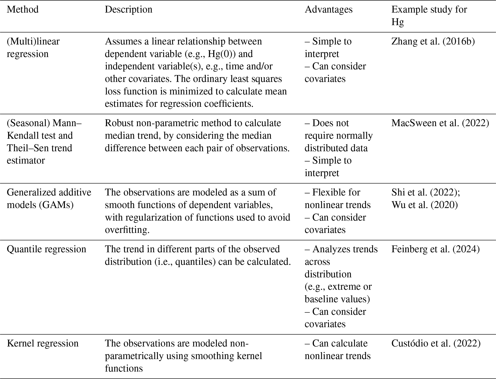
We would analyze trends in the baseline simulation A1 (Table F8) from available atmospheric Hg models, comparing these to observations of atmospheric Hg concentrations and deposition for 2010–2020. The baseline simulation would be conducted with drivers (i.e., anthropogenic emissions, legacy re-emissions, oxidant concentrations, and meteorology) that vary temporally over 2010–2020, representing the state-of-the-art knowledge for processes driving Hg cycling. Simulated trends at the grid cells of measurement stations will be extracted to compare with available measurements. We would evaluate the accuracy of the baseline models for capturing measured trends for 2010–2020, using an array of metrics (R2, mean absolute and relative biases, fraction of sites at which a model predicts the correct sign of a trend). The comparison of trends can be summarized for available observation media (Hg(0), THg, and Hg wet deposition) and specific regions where measurements are available.
Trends would also be compared between individual Hg models in the baseline simulation. In this analysis, we would not be limited to analyzing only areas where measurement stations are available. Modeled trends in atmospheric Hg concentrations will be calculated globally, over each hemisphere, and for all HTAP regions. Trends in Hg fluxes (e.g., dry deposition over land, wet deposition, and ocean–air Hg exchange) will be compared between models. Since all models will conduct simulations with harmonized emission datasets, differences between modeled trends will be attributed to other environmental drivers which will not be harmonized between models (i.e., meteorology, land surface parameters) and the individual parameterizations of Hg cycling. In addition, each individual model can conduct sensitivity simulations (A4.1–A5.10 in Table F8) using alternative anthropogenic and secondary emissions and parameterizations to diagnose the impact of these drivers on trends. This combination of intermodel and inter-simulation analysis will demonstrate the sensitivity of Hg trends to structural and parametric uncertainties in available Hg models. By comparing model temporal trends across global regions, uncertainty estimates in modeling results will be calculated and scientific gaps in modeling will be identified.
Attribution of trends
The proposed list of multimodel ensemble simulations would allow for attribution of Hg trends to individual emission sources and environmental drivers (Simulations A3a.1–A3b.7; see Table F8). For example, we will conduct a 2010–2020 simulation with fixed anthropogenic emissions at 2010 values (Simulation A3a.1). By comparing this simulation to the baseline simulation (A1, where anthropogenic emissions vary for 2010–2020), the influence of anthropogenic emission changes on Hg trends can be quantified. This attribution analysis can be conducted at different spatial scales (globally, hemispherically, regionally, and at locations of measurement stations) to better quantify the role of anthropogenic emissions in observed Hg trends.
Similar to the exercise proposed above for Simulation A3a.1, other drivers can be investigated by conducting simulations with 2010 fixed values. Simulations could be conducted to quantify the impacts of ASGM emissions (A3a.2), Annex D anthropogenic emission sources (A3a.3), and geogenic emissions (A3a.4). These sensitivity simulations would illustrate the roles of these diverse drivers in Hg trends between 2010 and 2020. Among other uses, the model products could be used to map the principal driver influencing Hg trends for each individual grid cell globally.
Effects related to the environmental conditions are difficult to disentangle, as many of the individual drivers (meteorology, land surface conditions, and secondary emissions) are intertwined. Additional optional simulations will probe the effects of changes in various environmental drivers on trends for diagnostic purposes. For these simulations, we will vary one driver between 2010–2020 and keep all other drivers fixed at 2010 levels. Proposed simulations will consider the effect in 2010–2020 trends of varying transport (A3b.1), wildfire emissions (A3b.2), terrestrial secondary emissions (A3b.3), ocean Hg concentrations (A3b.4), land surface conditions (A3b.5), chemical reactants (A3b.6), and anthropogenic emission speciation (A3b.7). The contributions of anthropogenic emission changes from different HTAP regions will be explored with Simulations A3c.1–A3c.11.
The model intercomparison will highlight whether the influence of drivers is comparable between the different models. Also, by analyzing the role of different trend drivers, we will be able to better understand differences in the modeled baseline trends and discrepancies between the models and observations. The previous global multimodel Hg study focused on an individual simulation year (Travnikov et al., 2017). Therefore, the transient 2010–2020 intercomparison simulations present a novel opportunity to evaluate the variety of model responses to changing Hg emissions and environmental drivers. In this way, MCHgMAP initiative will refine our understanding of the drivers of recent Hg trends and help with designing further simulations in subsequent EE efforts to isolate the impacts of MC and LRTAP activities on Hg trends.
Limitations and recommendations
Currently, the key limitations adding uncertainties to modeling trend analysis are the scarce information available regarding the trend in anthropogenic emissions from certain sources (e.g., for ASGM), geographically limited observations (mainly from North America and Europe) that cover the full 2010–2020 time period, and a lack of field or laboratory studies investigating the response of Hg fluxes (deposition and secondary emissions) to changes in environmental drivers. For example, the impact of land cover and vegetation properties on Hg uptake depends on model parameterizations of Hg(0) dry deposition calibrated to available field measurements (Zhou et al., 2021; Feinberg et al., 2022). However, there are few measurements of Hg vegetation uptake in tropical forests with high biological productivity, including no measurements in tropical regions of Asia or Africa. Although the proposed 10-year simulations would be longer than any previous Hg multimodel activity, the relatively short time period presents challenges to trend analysis owing to the role meteorological interannual variability in driving trends over shorter time periods as shown in studies using mechanistic modeling (Dastoor et al., 2022b) and statistical approaches (Shi et al., 2022; Wu et al., 2020).
A long-term Hg measurement record that is both regionally representative and process-representative and improved reporting of Hg emissions from various sectors can improve trend analysis in future EE efforts. Inverse models have been used in different atmospheric chemistry applications to calculate temporally and spatially varying emission fields using Bayesian inference and available observations (Bousquet et al., 2011; Park et al., 2021). Inverse modeling could aid in diagnosing changes in anthropogenic Hg emissions driven by the Hg MEA policies. However, until now, inverse modeling applications for Hg cycling have been limited in scope, both spatially and temporally (Song et al., 2015; Denzler et al., 2017). In the future, a diverse set of inverse Hg modeling methods could be applied to available atmospheric observations in order to produce estimates of Hg emission trends and their uncertainties.
7.2 Ocean
7.2.1 Current levels
The principal source of oceanic Hg is atmospheric deposition, air–sea exchange of gaseous elemental Hg(0), river input, and coastal erosion (Dastoor et al., 2022a; Amos et al., 2014; Mason and Fitzgerald, 1996). Much of oceanic Hg input is of anthropogenic origin (Driscoll et al., 2013), since the anthropogenic influence on global Hg cycling is significant. However, the response (time and level) of oceanic Hg levels to ongoing changes in anthropogenic emissions is currently uncertain. In addition to ongoing anthropogenic emissions, the oceanic response time is highly dependent on contributions from natural (geogenic) and historical (anthropogenic legacy emissions) sources (Zhang et al., 2014b). Thus, the design of MME simulation experiments needs to include ocean models that can track the contributions of different anthropogenic and geogenic sources of Hg emissions to water column Hg levels at observational sites and across global regions. The attribution of Hg emissions from different sources can be traced in several classes: geogenic, anthropogenic and secondary (separated by land, ocean, and wildfires); different anthropogenic Hg emission sectors; and anthropogenic Hg emission sources influenced by the MEAs.
Several previous modeling studies have focused on the impact of anthropogenic emissions on oceanic Hg levels (Chen et al., 2018; Corbitt et al., 2011). However, no 3D biogeochemical ocean model has been used to source-track Hg emissions over historic periods. Corbitt et al. (2011) used a tagged version of the GEOS-Chem model to track the fractional contribution of sources of atmospheric deposition to the surface ocean. Several previous modeling studies have examined the trends in evasion of Hg(0) from the oceans and their controlling factors: (i) global numerical models (Soerensen et al., 2010; Zhang et al., 2019c; Huang and Zhang, 2021), (ii) regional models (e.g., Fisher et al., 2013; Bieser and Schrum, 2016), and (iii) global box models (Mason and Sheu, 2002; Sunderland and Mason, 2007; Amos et al., 2013; Chen et al., 2018). It is estimated that the surface ocean Hg concentrations and its evasion into the atmosphere has increased by a factor of 3–5 since preindustrial times (Outridge et al., 2018; Zhang et al., 2014a; Huang and Zhang, 2021). Zhang et al. (2014b, 2016b) tracked the perturbation by anthropogenic Hg emissions in the past 600 years using a 3D ocean model and found that in surface waters 77 % of the Hg is of anthropogenic origin. Overall, modeling suggests that most of the Hg(0) being evaded comes from Hg that was recently added to the ocean (60 %–70 %), and that deeper water Hg sources are therefore a smaller component of the flux (Soerensen et al., 2010). Sunderland and Mason (2007) found that the contemporary ocean is not in a steady state with present-day atmospheric Hg inputs. Hg concentrations will therefore continue to increase, on average, if present-day emissions remain constant. If the ocean were to reach a steady state with present-day atmospheric Hg inputs, anthropogenic Hg enrichment would increase to ∼80 % in the surface ocean and >150 % in the deep ocean. Two-thirds of the present Hg fluxes (such as deposition on land and the ocean) are directly or indirectly of anthropogenic origin (primary or legacy anthropogenic emissions). Elimination of the anthropogenic load in the ocean and atmosphere will take hundreds of years if not more after the termination of all anthropogenic emissions (Amos et al., 2014).
Spatial pattern detection
The global distribution of aqueous mercury species in the ocean is determined primarily by the global patterns of (a) deposition, governed by location of emissions, atmospheric transport and reduction potential, (b) primary productivity, which affects the conversion of aqueous Hg(II) to Hg(0) and MeHg, (c) settling of Hg sorbed to organic particles, and (d) upwelling/resuspension of sedimented Hg. Gaining a comprehensive understanding of Hg levels and spatial patterns in the global ocean, especially in sensitive regions, is critical for accurately assessing the risk of human exposure and the reliability of the MC EE.
Moreover, deposition plays an important role in the distribution of Hg. Deposition is high in the western North Atlantic and western North Pacific, which are downwind of large industrial regions of the eastern US and East Asia (Strode et al., 2007). Due to increasing emissions from Asia and decreasing emissions from the US, deposition to the Atlantic has decreased while increasing in the Pacific over the last decades. These key regions, including the tropics, western North Atlantic and western North Pacific, should therefore be treated as “affected” by anthropogenic emissions. Also, for the tropics not located downwind of source areas, model simulations of Hg in the open oceans show elevated concentrations because of the prominent atmospheric deposition due to high precipitation in the Inter-Tropical Convergence Zone (ITCZ) in combination with increased atmospheric oxidation rates producing Hg(II) for dry deposition (Zhang et al., 2019c; Soerensen et al., 2014). While there are no large point sources of Hg in the Arctic, atmospheric transport of Hg(0) to this region still results in a significant anthropogenic impact to the Arctic Ocean (Schartup et al., 2022). Although considered as a “remote” region, Hg levels in the Arctic Ocean are therefore very sensitive to anthropogenic Hg emissions (Dastoor et al., 2022a). In the future, large quantities of Hg from thawing permafrost might be released into the Arctic.
The baseline simulation (O1, Table F9) aims to obtain global levels and spatial patterns of oceanic Hg utilizing state-of-the-art model configurations to perform global-scale simulations of oceanic Hg transport. The oceanic models incorporates boundary conditions (i.e., atmospheric Hg(0) concentrations, Hg(II) deposition fluxes, and Hg from rivers) from atmospheric and mass balance model results and present-day ocean biogeochemistry fields from ocean models such as Zhang et al. (2020) and Bieser et al. (2023). Due to the sparse nature of marine observations in general, and the lack of cruises during the stormy season and an absence of repeated (interannual and intra-annual) measurements in particular, a comprehensive evaluation of spatial patterns can only be achieved by combining observations and models. Here, the ensemble approach will help to reduce the uncertainty introduced by the models through the identification of regions of (dis)agreement between different models.
Attribution of levels
To comprehensively evaluate the contributions of various Hg sources to oceanic Hg levels and spatial patterns, simulations will be conducted using available ocean Hg models (O2.1–O2.6; Table F9). The contributions of geogenic and anthropogenic Hg emission sources (O2.1–O2.2) to oceanic total Hg concentrations at observation sites and across global regions will be determined by performing oceanic simulations using Hg deposition inputs from the respective atmospheric MME experiments (see Sect. 7.1.1). The oceanic models will be used further to identify the relative contributions of different anthropogenic emission sectors to oceanic Hg levels, such as the contributions of anthropogenic emissions from sources influenced by the MC (O2.5–O2.6). To account for non-atmospheric emission sources, the relative contribution of riverine input will be assessed using simulations with riverine emissions from Liu et al. (2021b) and without riverine export (O2.3). An additional experiment (O2.4) will investigate the contribution of Hg and MeHg bioaccumulation in marine biota in the lower food web (phytoplankton and zooplankton) to oceanic Hg distribution and air–sea exchange by disabling food web interactions.
Limitations and recommendations
A major limitation is the sparse availability of marine measurements of speciated Hg with large parts of the ocean still unsampled. From a model perspective, the chemical mechanisms for methylation and demethylation processes are still not understood. In the coastal ocean, the complex interactions between Hg and other components in river water and sediment, such as dissolved organic matter and suspended particles and biota have yet to be fully reproduced by a model. Assumptions made about key parameters in oceanic Hg biochemistry models introduce errors in the estimation of Hg cycling in the transition zone from freshwater to marine waters (e.g., change in pH).
Another limitation of current global ocean models is that they do not accurately represent coastal dynamics. Eddies are dissipated at much smaller scales than the grid resolution in the turbulent boundary layers, and advection schemes governed by turbulent mixing cannot be captured precisely by these coarse-resolution ocean models (Sarmiento et al., 2004; Wunsch and Ferrari, 2004). Furthermore, these models cannot adequately reflect transport and mixing conditions in the continental shelves as global models usually lack tides, which are major drivers of coastal mixing. Higher-resolution or unstructured grid models are necessary for capturing the complex processes at the land–sea–air interface. Here, we will perform additional runs evaluating the impact of model resolution. Models with unstructured grids will be used to selectively increase model resolution in coastal areas (Logemann et al., 2021). Furthermore, for the estimation of different source origins of oceanic Hg levels and their re-emission, there are computational problems with conducting historic (decennia or millennia) 3D model simulations, including source–receptor relationship tracking. For future EE efforts, we recommend that model simulations (mass balance models and fully coupled 3D models) with a focus on tracking Hg source origins (geography- and time-dependent) be developed further, building on the work of Corbitt et al. (2011), Amos et al. (2013), and Chen et al. (2018).
7.2.2 Temporal trends
The relevance of detecting and attributing changes in the concentration and distribution of Hg in the marine environment over time to the MC on Hg is significant. This can be accomplished using a combination of observational data, modeling studies, and statistical analyses. Estimates of temporal trends from observational data are not feasible due to the lack of long-term stations and sporadic cruising activity. However, ocean Hg models can be effective tools for addressing these gaps in our understanding of temporal trends in Hg levels in the ocean. Understanding the temporal trends provides a way to directly monitor progress towards reducing exposure to MMHg and other public health and the UN Sustainable Development Goals related to Hg pollution, particularly in coastal and indigenous communities that rely on fish and seafood as a primary food source. It is also essential for identifying changes in sources and pathways of ocean Hg levels, which can inform strategies for reducing anthropogenic Hg emissions and protecting human and ecosystem health.
Ocean Hg models have emerged as a powerful tool to provide valuable insights into the drivers and impacts of Hg pollution in the ocean over time. For example, 2D slab models of the oceanic mixed layer employed to mainly focus on air–sea exchange (Strode et al., 2007; Soerensen et al., 2010), only include inorganic Hg chemistry and transportation and use GEOS-Chem model results of atmospheric Hg. These are mainly concerned with seasonal temporal variability. Multi-box biogeochemical model (Soerensen et al., 2016a; Amos et al., 2013) are also developed to simulate Hg budget and response to emission inventory. Combined with projections of future anthropogenic Hg emission scenarios, Giang and Selin (2016) used Amos et al. (2013) and Schartup et al. (2022) used Soerensen et al. (2016a) to assess future changes in Hg levels. Three-dimensional biogeochemical models including ecosystem interactions are increasingly applied to simulate the spatiotemporal dynamics of Hg species in the ocean including bioaccumulation in the marine food web (Zhang et al., 2020; Rosati et al., 2022; Bieser et al., 2023; Zhu et al., 2023).
Trend detection
It is currently not possible to estimate temporal trends of oceanic Hg from observational data due to the lack of long-term monitoring and only sporadic cruising activity. Ocean Hg models are potent tools for filling the gaps in our knowledge of temporal trends of Hg levels in the ocean. Some models perform offline simulations for a certain amount of time with repeated external forcing from rivers and atmospheric deposition (Zhang et al., 2020), or fixed field (Rosati et al., 2022) or archived field (Bieser et al., 2023). Others are coupled to an atmospheric model using a monthly, weekly, or even hourly (Zhang et al., 2014b, 2019c) interval for data exchange. To capture the temporal trends associated with changes in emissions, the atmosphere–ocean coupled model simulations (discussed in Sect. 5) might provide a more justifiable time-dependent simulation than previous offline ocean model simulations.
Trends in the baseline simulation (O1; Table F9) of oceanic Hg models will be examined and compared to available measurements of Hg levels (e.g., THg or MMHg) in the ocean for 1980–2020 (when data are available, keeping in mind that these are sparse, especially for the early decades, and that clean sampling techniques had not always been introduced in early observation campaigns: see Sects. 4.3 and 4.4). The baseline simulation will be forced with upper-boundary conditions (i.e., atmospheric Hg concentrations and deposition fluxes) from atmospheric and mass balance models and ocean biogeochemistry fields from present-day situations to capture short- and long-term changes in oceanic Hg levels. The ocean physics field that is used to drive the transport of Hg in the models varies temporally over 1980–2020. We will extract simulated trends for those measurement locations where observational data spanning several years have been built up and compare them with the available measurement data. Statistical metrics such as R2 in regression analysis and the model performance evaluation criteria described in Sect. 6.2 will be applied to assess whether the baseline simulation can recapitulate the observed trend direction for the period 1980–2020.
Similar analysis will be applied to compare trends across multiple oceanic Hg models in the baseline simulation. The analysis will not be constrained to areas where measurements are available. Global trends will be calculated, along with trends for different regions and all oceans, rather than specific locations with observations. Differences in trends for Hg fluxes, such as sea–air exchange, particle sinking, and sedimentation will also be compared across different models. Through this comparative analysis, any differences or similarities in trends will be identified, providing insights into the underlying processes that drive these trends.
Attribution of trends
The proposed trend analysis perturbation simulations (O3.1–O3.14, Table F9) will enable the attribution of Hg trends to emission sources and environmental conditions in the ocean. The trend attribution analysis can be performed at different spatial scales (globally, hemispherically, regionally, and at observation locations). Perturbation simulation O3.1 allows for the separation of the impacts of changes in anthropogenic emissions and environmental factors. A 2010–2020 simulation will be conducted to examine the effect of changing meteorological conditions on oceanic Hg by keeping all other factors fixed to 2010 while changing the meteorological conditions. Furthermore, Simulations O3.3–O3.14 will estimate the influences of changes in anthropogenic emissions in various global regions on oceanic Hg trends. Comparison across multiple models will indicate whether the impact of drivers is similar among the models. Resolving the role of different drivers also provides an opportunity to better interpret biases between simulated baseline trends and observations, together with model differences. Through this attribution exercise, we aim to improve our understanding of the drivers that are responsible for the observed Hg trends in the ocean. This will aid in the design of future EE cycles, which will focus on isolating the impacts of Minamata Convention activities on Hg trends.
Limitations and recommendations
As the ocean has a much slower turnover time compared to the atmosphere, a time span of 10 years might be insufficient to detect certain trends at a significant level. This is especially true for Hg(II) methylation and bioaccumulation trends. Several Hg biogeochemical processes such as methylation or demethylation and sorption or desorption to organic material remain highly uncertain. Without proper parameterizations of these processes, it is difficult to accurately capture and attribute temporal trends. Finally, in this study independent models for atmosphere and ocean will be coupled through sequential iterations (see Sect. 5.1). In future EE efforts, fully interactive multimedia models should be developed and applied.
7.3 Environmental mass balance
The mass balance of budgets between environmental Hg sources (anthropogenic and natural), burdens, movements, and burial provide a quantitative summary of the global Hg cycling. The mass balance implies that changes in Hg levels in any environmental compartment of the biosphere over time would result in compensating changes in other interacting compartments. Thus, assessment of mass balance is useful for explaining the linkages between temporal trends of Hg in environmental matrices. Further, the knowledge of relative magnitudes of Hg budgets provides insight into how curbing anthropogenic Hg emissions under the MEAs is likely to affect Hg levels in different media.
Given the biogeochemical complexity and sparseness of Hg observations, global Hg budgets have been commonly reported based on 3D and multimedia mass balance model simulations using compilations of anthropogenic and natural Hg emissions (Outridge et al., 2018). However, increased observations during the last decade have enabled some observational budgets, notably for terrestrial–atmosphere Hg exchange (Sommar et al., 2020; Zhou et al., 2021; Zhou and Obrist, 2021) and marine Hg burden (Bowman et al., 2020). With increasing number and accuracy of models, modeling estimates of global atmospheric Hg budgets have been successively revised (Selin et al., 2008; Amos et al., 2013; Song et al., 2015; Cohen et al., 2016; Horowitz et al., 2017; Shah et al., 2021; Kawai et al., 2020; Zhou et al., 2021; Feinberg et al., 2022; Zhang and Zhang, 2022; Sonke et al., 2023). For example, updated understanding of vegetation and soil uptake of Hg(0) led to the revision of Hg(0) deposition budget to land up from 1200 (Horowitz et al., 2017) to 2850±500 Mg yr−1 (Sonke et al., 2023). The Hg mass balance for global ocean has been developed using 3D and mass balance models (Sunderland and Mason, 2007; Semeniuk and Dastoor, 2017; Zhang et al., 2019c), including interactions with marine biota (Zhang et al., 2020). On the regional scale, a combination of observations and models have been used to estimate Hg mass balance (Arctic: Soerensen et al., 2016a; Sonke et al., 2018; Petrova et al., 2020; Dastoor et al., 2022a; Mediterranean: Cossa et al., 2022; China: Feng et al., 2022a).
Reported global Hg budgets thus far are mostly based on individual modeling estimates. However, a combination of MME and observed estimates have been used to develop Arctic Hg mass balance (Dastoor et al., 2022a), which led to improved understanding of Arctic Hg cycling and key knowledge gaps in the region. In this study, global environmental budgets of total Hg (THg) (i.e., Hg anthropogenic and natural emissions and releases, loadings, and inter-media exchange and burial fluxes) will be developed based on the coordinated baseline MME simulation; budget details such as exchange fluxes for different land cover types and Hg speciation will be added. Since human exposure to Hg toxicity is dominated by the consumption of seafood, mass balance budgets of both THg and MeHg (the Hg form that bio-magnifies in food chains) in the global ocean will be developed. Range of uncertainties in global Hg budgets will be determined based on updated synthesis of monitoring data and multimodel experiments examining sensitivity to uncertainties in emissions and physical and biogeochemical processes.
The Hg mass balance uncertainty estimates developed in this study will help prioritize Hg monitoring and research areas. While there has been progress on observations of global air-vegetation-soil flux exchange, air-cryosphere and air–ocean–sediment Hg exchanges remain understudied. Hg stable isotopes studies have led to novel constraints on speciated Hg pathways in terrestrial ecosystems (Enrico et al., 2016; Obrist et al., 2017; Zhou et al., 2017; Yuan et al., 2019b); these methods can be further utilized to reduce errors in flux estimates of other matrices. Understanding the role of legacy Hg recycling is important for evaluating the recovery of environmental Hg under the MC implementation (Amos et al., 2013, 2015). Global-change-induced alterations in processes such as net primary production, wildfires, permafrost and sea ice cycles, and river discharge can significantly shift the global Hg mass balance (Denkenberger et al., 2012; Hsu-Kim et al., 2018; Schaefer et al., 2020). Diagnosing recent perturbations of global Hg mass balance due to climate change stressors is currently difficult due to a lack of long-term observations in key environmental matrices. Development of past Hg records from environmental archives and mechanistic 3D atmosphere–land–ocean biogeochemical Hg models would help in constraining the contemporary Hg mass balance and modeling its future trajectory under global change.
Mechanistic models integrate available knowledge of Hg sources and biogeochemical processes of environmental matrices to estimate Hg levels. Spatiotemporal inconsistencies of modeled Hg levels with observations suggests inaccuracies or knowledge gaps in primary drivers (emissions and releases and environmental conditions) and processes of Hg and their model representations. Sensitivity of modeled Hg levels to these inaccuracies or knowledge gaps can be diagnosed using model simulations and statistical analysis, guiding further development of Hg models, emission inventories, and field and laboratory studies investigating environmental Hg processes.
Limited progress on large-scale process-based terrestrial–hydrological modeling is recognized as an outstanding science gap here. Further research to monitor and model terrestrial Hg is critical for determining the lifetime and attribution (to anthropogenic and natural sources) of Hg in major terrestrial compartments and its coupling with atmospheric and marine Hg. Bishop et al. (2020) reviewed recent advances in terrestrial Hg cycling and recommended increased routine analyses of terrestrial Hg and process studies using isotopes and micrometeorological and microbial techniques to characterize spatiotemporal variations across the atmosphere–terrestrial–water interface. Also, increased measurements of Hg levels and mobilization properties at contaminated sites (e.g., industrial and mining operations, including ASGM) are required to adequately represent their role in releasing Hg into the atmosphere and global surface waters. Sonke et al. (2023) recommended monitoring of Hg concentrations in major regional rivers and their tributaries to assess the integrated influences of global change on terrestrial Hg cycling. In the following sections, atmospheric and oceanic model simulations probing Hg process understanding are discussed.
8.1 Atmospheric models
Previous modeling studies have explored the influence of anthropogenic forcing on the simulation of atmospheric Hg concentration and deposition. Uncertainties in atmospheric Hg emission inventories impact the prediction of source–receptor relationships of Hg (De Simone et al., 2016, 2017a), which are important for estimating the impacts of MC policy on the global distribution of Hg deposition. Previous studies have used models to evaluate Hg emission inventories against observational evidence (Hg air concentrations and deposition). The impacts of Hg speciation (Hg(0) vs. Hg(II)) in emission inventories was analyzed by Bieser et al. (2014), Zhang et al. (2016b), and Giang et al. (2018), finding that accurate representation of emission speciation is crucial for capturing the impacts of Hg emission reductions on atmospheric Hg concentrations and deposition. The impacts of other types of anthropogenic forcing (e.g., land use change) have been less frequently investigated. Previous generations of models showed limited impacts of future land cover and vegetation change on atmospheric Hg (Zhang et al., 2016a), yet these models likely underestimated the importance of Hg(0) dry deposition in the global Hg budget (Zhou et al., 2021; Feinberg et al., 2022). A recent modeling study implied that land use change impacts on atmospheric Hg deposition can be on par with direct anthropogenic emission impacts (Feinberg et al., 2023). The choice of other input driver datasets can play a role in simulated Hg cycling, including the choice of meteorological input data (Dastoor et al., 2015; Giang et al., 2018).
The prediction of atmospheric Hg cycling depends not only on the input driving datasets, but also on the design of the model parameterization of Hg biogeochemistry. There are several published studies investigating the impact of the Hg chemical scheme on the spatial distribution and seasonality of Hg concentrations and deposition (Saiz-Lopez et al., 2020, 2018; Ye et al., 2018b; De Simone et al., 2017a; Travnikov et al., 2017). The parameterizations of air–surface exchange also play an important role in the emissions and fate of atmospheric Hg. Zhang et al. (2019c) tested five parameterizations of air–sea Hg(0) exchange, determining that global net Hg(0) emissions range between 2840 and 3710 Mg yr−1, with strong regional differences between parameterizations. The choice of Hg(0) dry-deposition parameterization can strongly impact the magnitude of Hg(0) uptake by vegetation (Zhou et al., 2021; Feinberg et al., 2022). Even with the same model parameterizations, the horizontal resolutions of Hg models can impact the simulation of wet deposition due to finer-resolution models being better able to capture deep convection (Xu et al., 2022; Zhang et al., 2012).
By constructing simulations in a diverse set of atmospheric Hg models with updated harmonized boundary conditions, we can identify current knowledge gaps in the biogeochemical Hg cycle and test key uncertainties in available models. Sensitivity and uncertainty simulations will provide further insight into the drivers of Hg trends and spatial distribution and inspire further developments to improve cause–effect relationships in Hg cycling.
MCHgMAP will explore the impacts of several anthropogenic and environmental forcing factors on Hg cycling. In addition to the previously discussed baseline (A1) and trend analysis (A3a.1–A3b.7) simulations for 2010–2020, an array of atmospheric model simulations is proposed to test the influence of alternative emission datasets and parameterizations (A4.1–A4.8). Additional idealized sensitivity simulations (A5.1–A5.10) are proposed to investigate the sensitivity of Hg model budgets in a single year (2015) to individual processes. This set of simulations is idealized in the sense that rough perturbations are imposed on drivers (e.g., A5.1: all Hg emissions are released as Hg(0)) or model parameters (e.g., A5.3: enhancing Hg oxidation rates by +50 %). These experiments can probe whether existing models differ in their sensitivities to individual drivers or biogeochemical parameters, enabling the prioritization of key uncertainties for future EE efforts. The idealized experiments can also explore potential impacts of future global change, e.g., increases in LAI due to global greening (A5.8) or the disappearance of sea ice (A5.10).
Currently, there are limited options for anthropogenic Hg emission inventories, especially continuous time series using a consistent methodology covering the years 2010–2020 or longer (see Sect. 3.2.1), restricting the ability to investigate emission uncertainties and sensitivity to modeling results. Chemical mechanisms differ among the models because of knowledge gaps and uncertainties in atmospheric Hg and Br chemistry, but the interpretation of differences in model-simulated chemistry is made more difficult due to limited observations of speciated Hg and potential biases in these observations (Lyman et al., 2020a). Finally, the sensitivity analysis performed with atmospheric models decoupled from the aquatic and terrestrial compartments does not account for changes in Hg levels in other environmental media affecting secondary emissions to the atmosphere. The internal consistency of this analysis would be improved by Hg simulations in Earth system models (e.g., Zhang and Zhang, 2022), yet the computational expense of dynamically coupled models implies that atmosphere-alone sensitivity simulations are worthwhile for probing process uncertainties.
8.2 Ocean models
Previous single model process studies have investigated (1) the impact of riverine Hg loads (Fisher et al., 2012; Soerensen et al., 2012; Zhang et al., 2015b), (2) the role of organic matter in marine Hg cycling and methylation (Soerensen et al., 2016a), (3) air–sea exchange (Bieser and Schrum, 2016; Zhang et al., 2023a), (4) the impact of nutrients on methylation and bioaccumulation (Soerensen et al., 2016b), and (5) the impact of adding interactions with the marine ecosystem (Zhang et al., 2019c; Rosati et al., 2022; Bieser et al., 2023). However, so far, no systematic model intercomparison or ensemble study has been performed for oceanic Hg cycling. MCHgMAP will, for the first time, use a set of marine Hg models driven by harmonized input data and model parameterizations. Thus, the baseline (O1) scenario (Table F9) will be used to quantify the range of currently available models (Table F2) based on harmonized input data and process parameterizations (Table F6). So far it is unknown how marine Hg models compare and whether spatial or seasonal patterns are in model (dis)agreement.
The initial evaluation will focus on comparing the baseline scenario model simulations to identify regions, times, and species for which the model's baseline results differ (see Sect. 6.2). The models will be evaluated against observations with a focus on regions and species where models are not in agreement with each other. The initial evaluation will also include hydrodynamic (e.g., circulation patterns, overturning time, regional stratification and upwelling) and biogeochemical (e.g., nutrients, phytoplankton and zooplankton concentrations and seasonality) variables so as to understand the discrepancies of non-harmonized internal model processes. Further, a range of simulations (O4.1–O4.7) attributing uncertainties to individual external and internal modeling factors are proposed.
-
Anthropogenic emissions: the model uncertainty due to emission inventories and speciation will be estimated using different atmospheric Hg boundary conditions from the atmospheric models. For this, there are three scenarios (O4.1–O4.3) using alternative anthropogenic emission inventories as model drivers. This will help in understanding the uncertainty due to Hg total emission, and their spatial distribution and speciation. The latter is of special importance, as Hg speciation in emission, especially from the largest source sector of coal combustion, has been changing due to new technologies such as desulfurization. Depending on the fraction of Hg emitted in oxidized or particulate form, even the identical total Hg emissions can lead to vastly different spatial distributions of Hg deposition to global oceans since the atmospheric lifetime of elemental Hg(0) is an order of magnitude higher than that of the other species.
-
Methylation–demethylation: the exact processes that govern methylation and demethylation are still not fully understood. To better understand the model uncertainty due to different chemical mechanisms for Hg transformation, scenario O4.4 tests the impact of the chemical mechanism by harmonizing reactions and rates for Hg transformations.
-
Air–sea exchange: with an annual Hg net evasion of 3000–4000 Mg from the ocean, this is the largest Hg flux into the atmosphere. However, this process is not well understood and only indirectly observable. Estimates of global air–sea exchange are based on either co-located Hg(0) measurements in the air and surface ocean or from global atmospheric models. Simulations O4.5 and O4.6 will use alternative parameterizations for the two-layer air–sea exchange model to estimate the uncertainty due to this process. Moreover, by coupling to the atmospheric models, we will create consistent multi-compartment estimates, taking into account atmospheric and marine processes and quantifying the model uncertainty due to the air–sea exchange parameterization.
-
Model resolution: simulation O4.7 examines the impact of marine model resolution. This is of interest as low resolution global models cannot resolve the coastal shelf seas. However, these regions have the largest biological productivity and are thus potentially both an important sink for Hg and a region of enhanced methylation. The impact of the shelf oceans and the necessity of high-resolution ocean models to resolve this process for carbon cycling was recently shown by Mathis et al. (2022).
-
Secondary emissions: a central question in the global Hg cycle is what fraction of marine Hg evasion into the atmosphere stems from previously deposited anthropogenic Hg emissions. This secondary emission fraction will be estimated based on Simulations O2.1 and O2.2, where contemporary anthropogenic and geogenic emissions are zeroed out.
-
Bioaccumulation: the central reason for nations to agree on the MC is the threat to human health posed by Hg and MeHg in seafood. With biogeochemical marine Hg models, it is possible to quantify methylation and uptake of Hg in the marine ecosystem and the impact of external stressors like anthropogenic emissions and climate change thereon. Understanding the influence of biotic Hg is important for the distribution of oceanic Hg. For example, a recent study (Amptmeijer and Bieser, 2023) shows that Hg uptake by phytoplankton can lead to higher MeHg concentrations in the surface ocean as well as increased Hg(II) sedimentation and Hg(0) air–sea exchange. Simulation O2.4 investigates the role of Hg bioaccumulation in the lower food web (phytoplankton and zooplankton) and sedimentation of Hg sorbed to organic particles on marine Hg.
Within the limitations and uncertainties outlined above, and quantified through the proposed simulations, models are essential tools for projecting future trajectories of Hg levels in the air and ocean. This includes projecting the influence of scenarios of implementation of the MC and other MEAs, as well as changes in Hg levels that result from changing environmental conditions (due to climate and other global changes).
Appropriate methods for modeling changes in atmosphere and ocean Hg levels depend strongly on the timescale of interest. With respect to the immediate time frame of the first MC EE, projecting changes over a few years requires consideration of changes in the contemporary cycle (see Fig. 1). For changes over several years to decades, the long-term cycle becomes increasingly relevant (Amos et al., 2013). It is important to note that changes to the long-term cycle that affect atmospheric and ocean Hg concentrations on timescales of several years or more are driven not only by past emissions, but also by the cycling of ongoing and future Hg emissions (Selin, 2018).
A number of previous studies have used atmospheric models to project atmospheric concentrations of Hg and changes in wet and dry deposition, under future conditions and both regionally and globally. Pacyna et al. (2016) used two global chemical transport models (GLEMOS and ECHMERIT) to project changes in future Hg concentrations and deposition at a global scale under policy scenarios relating to current pollution control and climate policies. Angot et al. (2018) simulated the same emission scenarios using the GEOS-Chem model. Other efforts have also drawn on global scenarios to quantify potential changes in source–receptor relationships (Chen et al., 2018; Corbitt et al., 2011; Zhang et al., 2021a) and regional impacts (Giang et al., 2015; Lei et al., 2014; Schartup et al., 2022). Regarding the ocean, there are fewer existing studies that project future ocean Hg concentrations in different scenarios (consistent with the more general limitation in the number of models that exist, as noted in Sect. 2.2). Zhang et al. (2021b) simulated five different future anthropogenic emission scenarios (ranging from a >80 % reduction to a 2.5-fold increase) using a coupled 3D atmosphere–ocean model. A recent assessment of the Arctic environment simulated likely changes in both atmospheric and oceanic Hg there in future emission scenarios (Schartup et al., 2022).
A few attempts have used various degrees of model coupling to address the combined impact of future and legacy changes, accounting for the influence of future emission scenarios on the long-term cycle. One study calculated that extending emission reductions over 5 years led to a 14 % decrease in local-scale Hg deposition (Angot et al., 2018). These estimates are affected by the uncertainties in timescales of inter-compartmental cycling and the overall mercury budget: Zhang et al. (2023a) recently calculated a lower sensitivity of atmospheric levels to anthropogenic emissions than had been estimated in previous models, due to a larger role of legacy emissions from the terrestrial and marine environments.
Section 3.2.2 (“Future emissions”) outlines progress towards developing future emission scenarios for Hg that leverage the best-available information on trajectories of different economic activities (including related efforts to limit greenhouse gas emissions by reducing fossil fuel use) with updated data on control measures. Understanding the relative importance of each of these drivers through different emission scenarios (Table E12) will be important for differentiating the influences of Minamata-related legislation, ambitious end-of-pipe control measures, and net-zero climate targets on levels of Hg in the atmosphere and ocean.
Simulations A6.1–A6.3 are designed to provide information on the relative impact of changes in atmospheric concentrations of mercury resulting from changes in anthropogenic emissions, environmental factors, and combined influences. Because each model setup is different, it will be important in these simulations to clearly differentiate how the impacts of past and future emissions are treated, the latter of which will also influence long-term cycling, as well as the source of future environmental conditions. For those scenarios that do not account of the time-varying legacy contribution from future scenarios, they will reflect a lower bound. As the impact of different sources adds linearly in the global mercury cycle, it will also be possible to derive source–receptor relationships useful for policy and future evaluation from the additional atmospheric simulations for the present (an example of such a strategy is presented by De Simone et al., 2020). In this study, we can update the legacy emission estimates for the atmospheric models by offline coupling to the ocean and making use of mass balance models. For the marine model simulations, O5.1–O5.3 will mirror the atmospheric setup. To allow for the identification of significant trends, the simulation will cover a time span of 30 years.
Scenario A2.1, the perturbation simulation with no anthropogenic emissions, will also be informative in understanding and bounding the potential for anthropogenic actions to affect mercury concentrations. Examining the model response to these scenarios, particularly with coupled and multimedia simulations, will provide important uncertainty bounds on future policy-relevant analysis. Quantifying the mercury response to zeroing-out emissions will be an important metric through which to compare model processes, similar to the zero-emissions commitment (ZEC) concept used for Earth system models for CO2 (MacDougall et al., 2022).
In all future scenarios, it will also be important to account for variability (especially with respect to future climate influences). While single-year constant meteorological comparison is appropriate for evaluating impacts of near-term emission changes, multiple years or even decades of simulation will be required to account for natural variability in the climate system and its influence on atmospheric chemical processes (Garcia-Menendez et al., 2017; Giang et al., 2018). In addition, differences among models reflect systematic uncertainties in key processes underlying the mercury cycle. Moving forward, model intercomparisons and model analysis in combination with increasing data constraints, including through the activities proposed above, will help narrow key uncertainties that hamper current ability to project future scenarios.
The Multi-Compartment Hg Modeling and Analysis Project (MCHgMAP), an international ensemble modeling initiative to inform the effectiveness evaluations of the Minamata Convention on Mercury and the Convention on Long-Range Transboundary Air Pollution, has been introduced. The MCHgMAP is intended to address the key policy questions of these multilateral environmental agreements (MEAs) by using an up-to-date Hg modeling capacity. (1) What are the contributions of anthropogenic emissions and releases and other Hg sources to current Hg levels observed in the air, biota, humans, and other media? (2) How have these contribution levels changed over time and over the timeline of the MEA? (3) How do the contribution levels and their trends vary geographically at the global scale? (4) What are the contributions of anthropogenic emissions and releases and other drivers to the temporal trends in observed Hg levels across global regions? (5) How are observed Hg levels expected to change in the future?
This overview paper is an important preparatory stage of the MCHgMAP, which will be followed by individual publications on different aspects of the study. Sections 1 to 4 provide a synthesis of what is currently known and not known about the estimates of mercury primary and secondary emissions, observations (direct monitoring and natural archives) and single- to multi-compartmental mercury models, and how these advances can be exploited to develop mechanistic understanding of the past, present, and future fates of environmental mercury. The project aims at improving comparability across the participating models by employing a consensus set of emissions and environmental conditions (where possible), and constraining model evaluation with common observation datasets. Methodologies for developing harmonized model drivers including historical and future primary and secondary emissions as well as biochemical fields that can be used in core and optional simulations are described. Sections 5 and 6 describe the rationale, design, implementation, and evaluation of multimodel experiments. The subsequent Sects. 7 to 9 present analysis of modeling results, i.e., detection and attribution of spatial patterns and temporal trends, identification of uncertainties, and future projections, to address the policy questions. Additionally, all sections provide recommendations for the areas of mercury research (monitoring and modeling) that are needed to improve effectiveness evaluations of the Hg MEAs going forward.
A challenge of analyzing the fate of emitted mercury is that it can recycle between the atmosphere, land, and ocean (i.e., secondary emissions and releases), and as a result, past and present emissions can continue to affect the environment on timescales of decades to centuries. There have been significant developments in marine and land Hg observations and modeling since previous ensemble Hg modeling studies which were mainly focused on atmospheric processes. Availing new advances, the MCHgMAP utilizes a coordinated simulation approach between single medium (atmosphere, land, and ocean) and multimedia Hg models to allow and measure the influence of changes in secondary Hg exchanges on environmental Hg cycling. The MCHgMAP baseline and perturbation ensemble simulations are designed to robustly analyze global and regional environmental Hg levels, i.e., detection and attribution of spatial gradients and temporal trends, understanding of global mass balance between sources, sinks and burdens, and future projections under different scenarios of implementation of the Minamata and other MEAs and changing environmental conditions. Additional model experiments, uncertainty and idealized, are designed to assess the sensitivity of modeled levels and trends to their drivers and underlying processes to guide future developments of emission inventories, and field and laboratory studies investigating environmental mercury. Finally, the model experiments are prioritized into three tiers – core, optional, and future simulations – to ensure a systematic and comprehensive analysis and flexibility in the plan to encourage participation of a variety of mercury models from the scientific community.
The coordinated multimedia, multimodel simulations in MCHgMAP are designed to analyze current and future levels and temporal trends of environmental Hg on global and regional scales to inform the effectiveness evaluations of the MC and LRTAP conventions. The MCHgMAP activities are targeted to address the following policy questions (divided into six categories), in alignment with the objectives outlined in the Minamata monitoring guidance UNEP/MC/COP.4/INF/12 (Guidance on monitoring mercury and mercury compounds to support the effectiveness evaluation of the Minamata Convention|Minamata Convention on Mercury, 2023) and the data analysis plan of the MC Open-Ended Science Group (UNEP/MC/COP.5/INF/24). The first set of questions is aimed at developing and/or examining the levels and trends of environmental Hg drivers, i.e., primary and secondary Hg emissions and releases and environmental conditions. The next five categories of policy questions address the analysis of environmental Hg spatiotemporal patterns and trends, i.e., their detection, attribution, process understanding, future projections, and mass balance budgets. In the following list, “mercury levels” refers to Hg concentrations and/or fluxes.
- A.
Driving sources and environmental conditions of environmental mercury
-
What are the current levels and temporal trends of primary Hg emissions and releases from anthropogenic and natural sources across the globe?
-
What are the current levels and temporal trends of secondary Hg emissions and releases from biomass burning, soils, and oceans across the globe?
-
What are the current levels and temporal trends of environmental variables related to Hg processes across the globe?
-
What are the fractional contributions of changes in anthropogenic Hg emissions and releases and environmental conditions to changes in secondary Hg emissions and releases over the period ca. 2010 to present across the globe?
-
How are anthropogenic Hg emissions and releases expected to change in the future in different scenarios of implementation of the Minamata and other conventions across global regions?
-
How are secondary Hg emissions and releases from biomass burning, soils, and oceans expected to change in the future under changing anthropogenic Hg emissions and releases and environmental conditions across global regions?
-
- B.
Detection of spatiotemporal features of environmental mercury
- 7.
What are the spatial patterns and temporal trends of Hg levels in the air and ocean across the globe?
- 8.
What is the spatial representativeness of current levels and temporal trends of Hg observed in the air and ocean?
- 9.
How are spatial patterns and temporal trends of Hg levels in the air and ocean related to patterns and trends of other pollutants or environmental variables on the global scale?
- 7.
- C.
Attribution of spatiotemporal features of environmental mercury
- 10.
What are the fractional contributions of primary (anthropogenic and natural) and secondary Hg emissions and releases to current Hg levels observed in the air and ocean across global regions?
- 11.
How have the fractional contributions of primary (anthropogenic and natural) and secondary Hg emissions and releases to levels of Hg observed in the air and ocean changed over the period ca. 2010 to the present across global regions?
- 12.
What is the fractional contribution of anthropogenic Hg emissions influenced by the convention to current Hg levels observed in the air and ocean across global regions?
- 13.
How has the fractional contribution of anthropogenic Hg emissions influenced by the convention to Hg levels observed in the air and ocean changed over the period ca. 2010 to the present across global regions?
- 14.
What are the fractional contributions of changes in primary anthropogenic and natural Hg emissions and releases and environmental conditions to changes in Hg levels observed in the air and ocean over the period ca. 2010 to the present across global regions?
- 15.
What is the fractional contribution of changes in anthropogenic Hg emissions influenced by the convention to changes in Hg levels observed in the air and ocean over the period ca. 2010 to the present across global regions?
- 16.
In each world region, how much of the contribution of changes in primary anthropogenic Hg emissions to changes in Hg levels observed in air over the period ca. 2010 to the present are due to emissions within the region versus outside the region?
- 10.
- D.
Estimation of mass balance budgets of environmental mercury
- 17.
What is the global mass balance of Hg between budgets of emissions, releases, levels, and movements in the environment?
- 17.
- E.
Process understanding of environmental mercury
- 18.
How consistent are the spatial patterns and temporal trends of Hg levels observed in the air and ocean with estimates from current mechanistic models across global regions?
- 19.
How consistent are the anthropogenic emission inventories and inventory data with spatial patterns and temporal trends of Hg levels observed in the air and ocean on the global scale?
- 20.
How sensitive are the spatial patterns and temporal trends of Hg levels in the air and ocean to various primary and secondary Hg emissions and releases as well as environmental conditions across global regions?
- 21.
How sensitive are the spatial patterns and temporal trends of Hg in the air and ocean to various Hg processes across global regions?
- 18.
- F.
Future projections of environmental mercury
- 22.
How are Hg levels in the air and ocean expected to change in the future in different scenarios of implementation of the Minamata and other conventions across global regions?
- 23.
How are Hg levels in the air and ocean expected to change in the future under changing environmental conditions across global regions?
- 22.
The exchange of mercury between the ocean and the atmosphere plays an important role in the cycling of mercury in the global environment. Available parameterizations of mercury air–water exchange used in modeling and measurement studies still vary considerably indicating an incomplete understanding of the process and lack of direct measurements. We here present the parameterizations recommended for use in the MCHgMAP multimodel experiments.
The two-layer (film) model by Liss and Slater (1974), which is the traditional parameterization used to determine the Hg air–water gas exchange flux, is recommended. It is possible to neglect the gas-side part of the transfer velocity in the model as the gas-side conductance for Hg is much higher than that on the water side () (Nerentorp Mastromonaco et al., 2017a). We further recommend the parameterization of the gas transfer velocity (kw) by Wanninkhof (2014) that is based on the updated methodology of Wanninkhof (1992) and that is in close agreement with parameterizations based on gas exchange process studies over the oceans (e.g., Nightingale et al., 2000a, b) (Fig. B1). Recent micrometeorological measurements by Osterwalder et al. (2021) provide estimates of kw determined directly for Hg. However, this is the first time that this method has been used for Hg flux evaluation, and more measurements are needed to validate the result. Therefore, the application of this alternative parameterization is only recommended for uncertainty analysis.
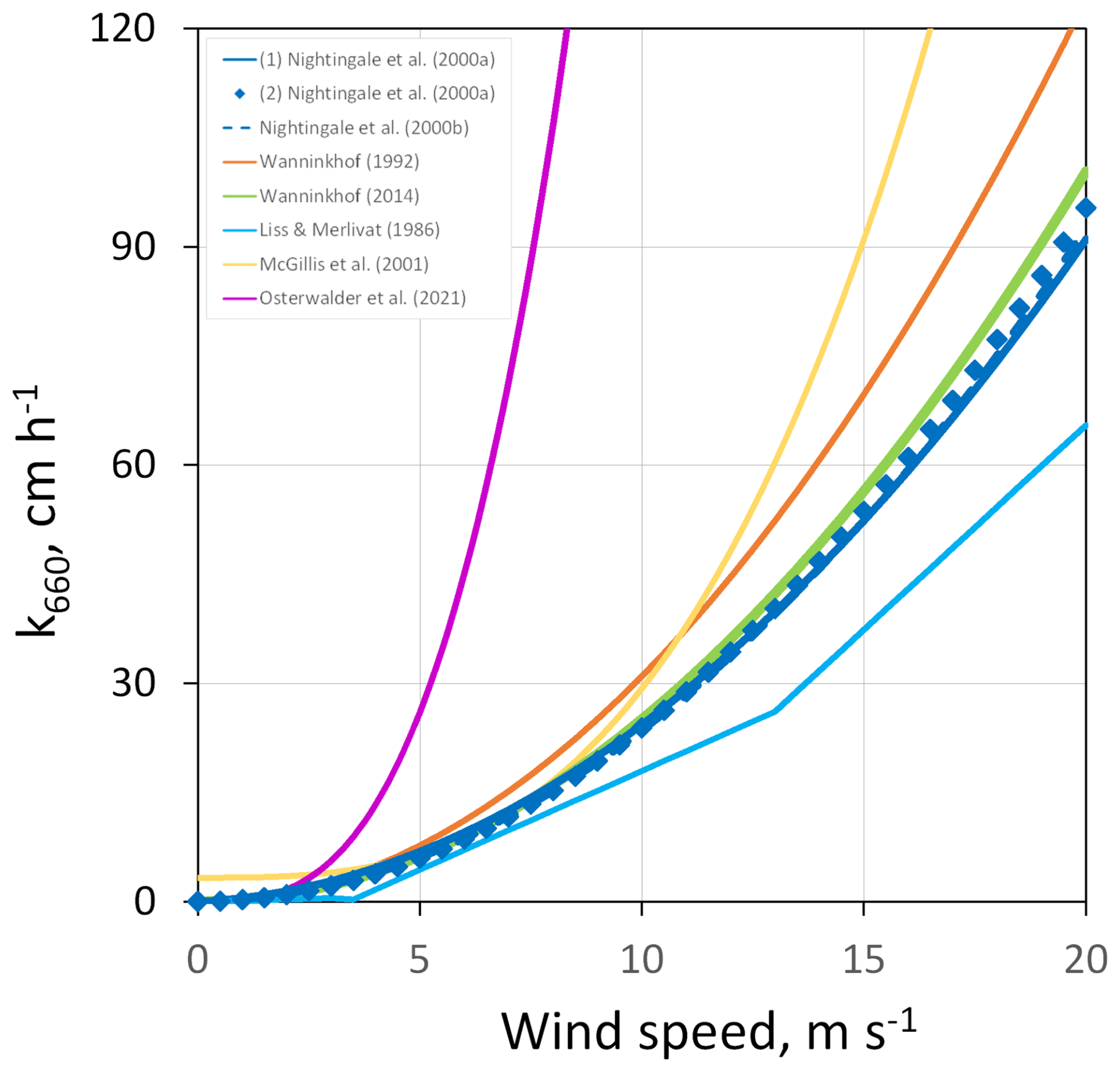
Figure B1Wind speed dependence of air–water gas transfer velocities from various parameterizations often applied in Hg modeling and measurement studies scaled to a Schmidt number of 660 (CO2 in seawater at 20 °C). Nightingale et al. (2000a) parameterizations 1 and 2 (in solid dark blue) are both commonly used in Hg work and give almost identical results. The dark-blue dotted line refers to Nightingale et al. (2000b), the orange line to Wanninkhof (1992), the green line to Wanninkhof (2014), the light-blue line to Liss and Merlivat (1986), the yellow line to McGillis et al. (2001), and the pink line to Osterwalder et al. (2021).
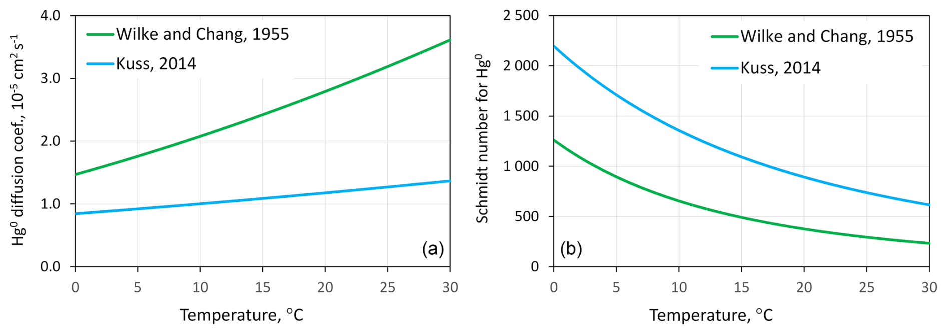
Figure B2(a) Temperature dependence of the Hg0 diffusion coefficient. (b) Temperature dependence of the Schmidt number of Hg(0) in seawater (from Wilke and Chang (1955) in green and Kuss (2014) in blue).
The temperature dependence of the gas transfer velocity of Hg is defined by the Schmidt number of Hg (Schmidt number is a ratio of water kinematic viscosity to the diffusion coefficient of a gas). The biggest differences between available parameterizations for the Schmidt number of Hg relate to the diffusion coefficient of Hg(0). For the diffusion coefficient of Hg(0) in the baseline simulations, we recommend the widely used parameterization by Wilke and Chang (1955). An alternative choice for sensitivity tests is the experimentally determined approximation from Kuss (2014), which provides lower values for the diffusion coefficient and consequently larger values for the Schmidt number (Fig. B2). Parameterizations of water kinematic viscosities by Kestin et al. (1978) and Sharqawy et al. (2010; freshwater and saltwater versions) do not differ significantly from each other. Of the two available parameterizations of the water kinematic viscosity for seawater (Wanninkhof, 1992; Sharqawy et al., 2010), we suggest the latter to be more universal since it provides values for a wide range of salinity. Figure B3 shows the temperature dependence on the transfer velocity for parameterizations recommended compared to the alternative combination.
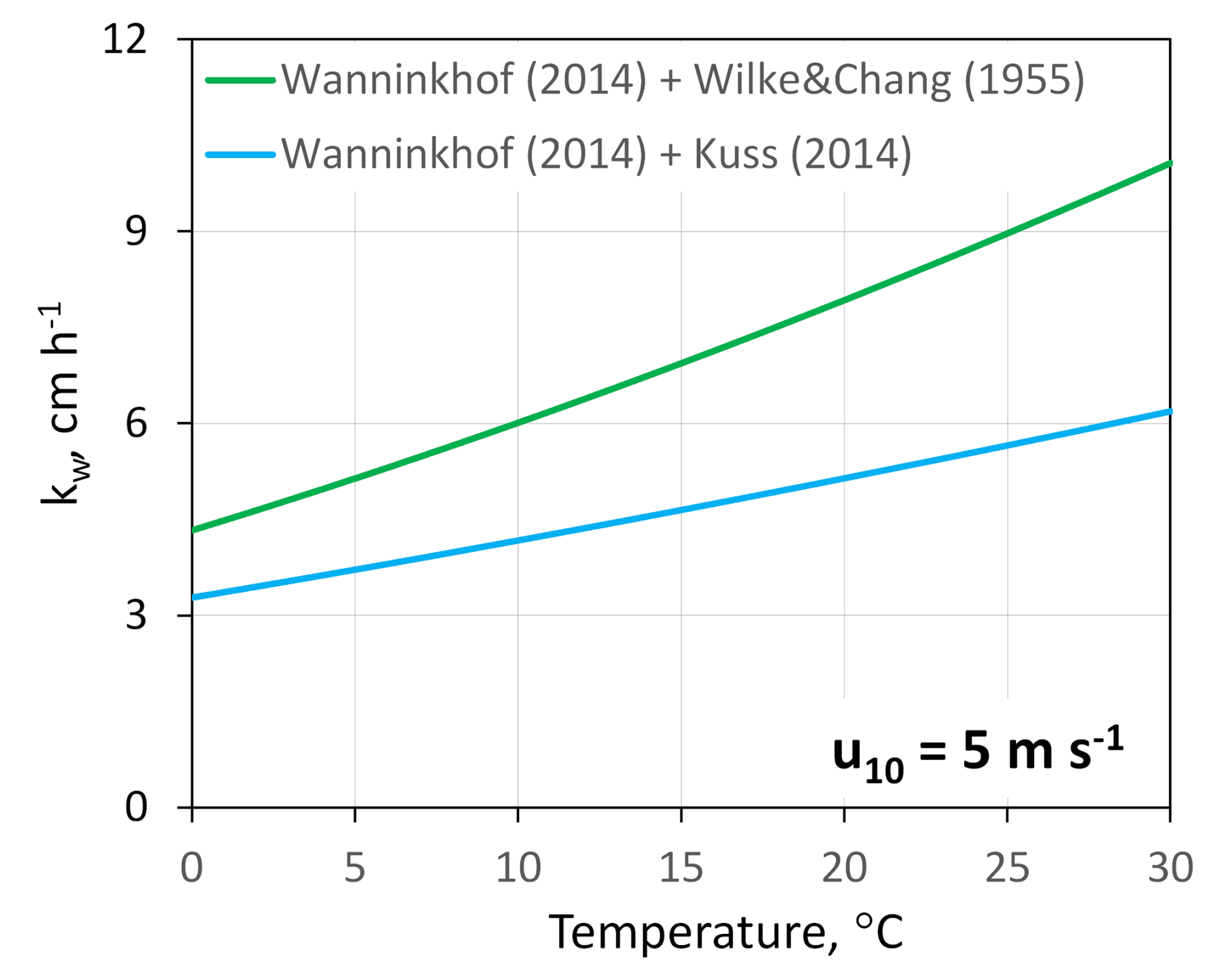
Figure B3Temperature dependence of air–seawater gas transfer velocity for Hg(0) (from Wilke and Chang, 1955, and Wanninkhof, 2014 – green; Kuss, 2014, and Wanninkhof, 2014 – blue).
The equations below outline all recommendations for Hg(0) air–water exchange parameterizations for the model experiments under MCHgMAP. Parameterization of Hg(0) exchange flux between air and seawater (S=35 g kg−1) approach:
ca and cw are concentrations of Hg(0) in air and water [ng m−3].
(Andersson et al., 2008a). T is the water temperature [K].
(Wanninkhof, 2014). u10 is wind speed at 10 m height [m s−1].
(Sharqawy et al., 2010).
t is water temperature [°C];
(Wilke and Chang, 1955). T is the water temperature [K]; Φw=2.26 is the solvent association factor (Hayduk and Laudie, 1974); Mw=18.01 is the molecular weight of water [g mol−1]; Vb=12.74 is the molar volume of mercury at its normal boiling temperature [cm3 mol−1] (Loux, 2004; Soerensen et al., 2010); η=ηswis the dynamic viscosity of seawater [g cm−1 s−1].
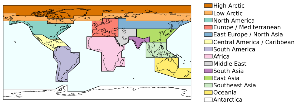
Figure C1Geographical source and receptor regions for atmospheric model analysis.
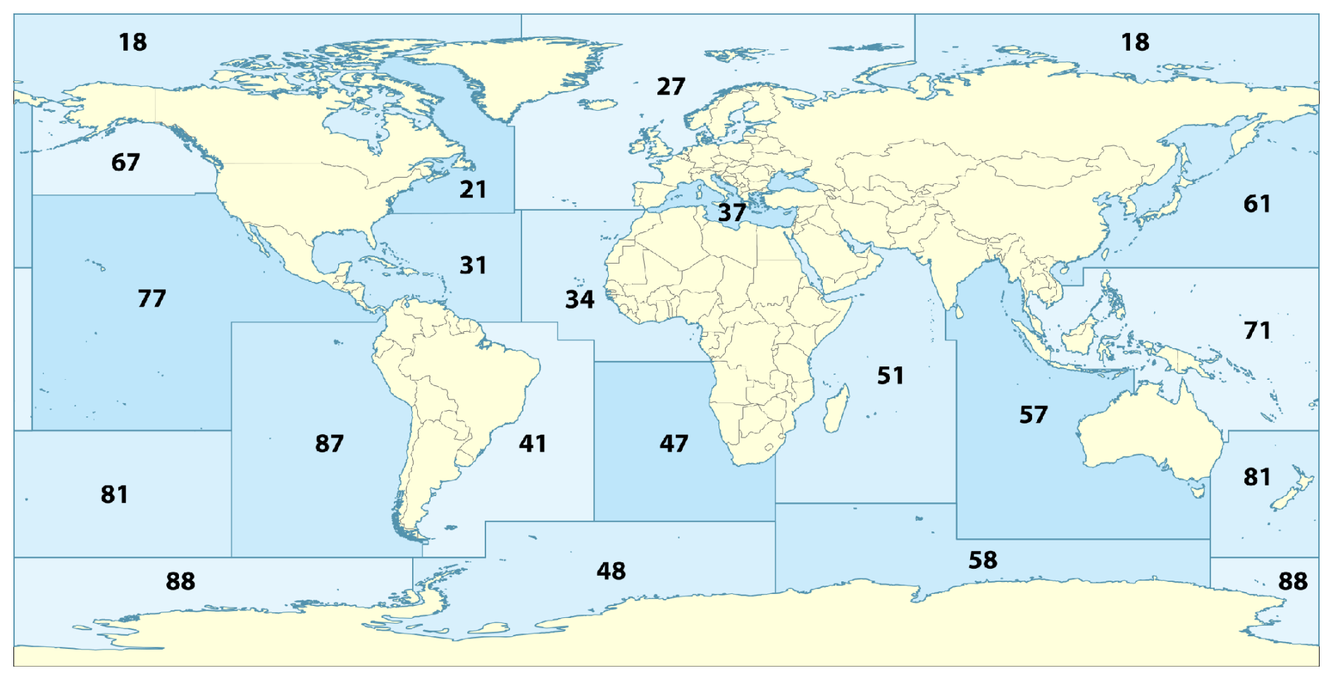
Figure C2Aquatic receptor regions for ocean model analysis (FAO major fishing areas, https://www.fao.org/fishery/en/area/search, last access: 1 May 2025).
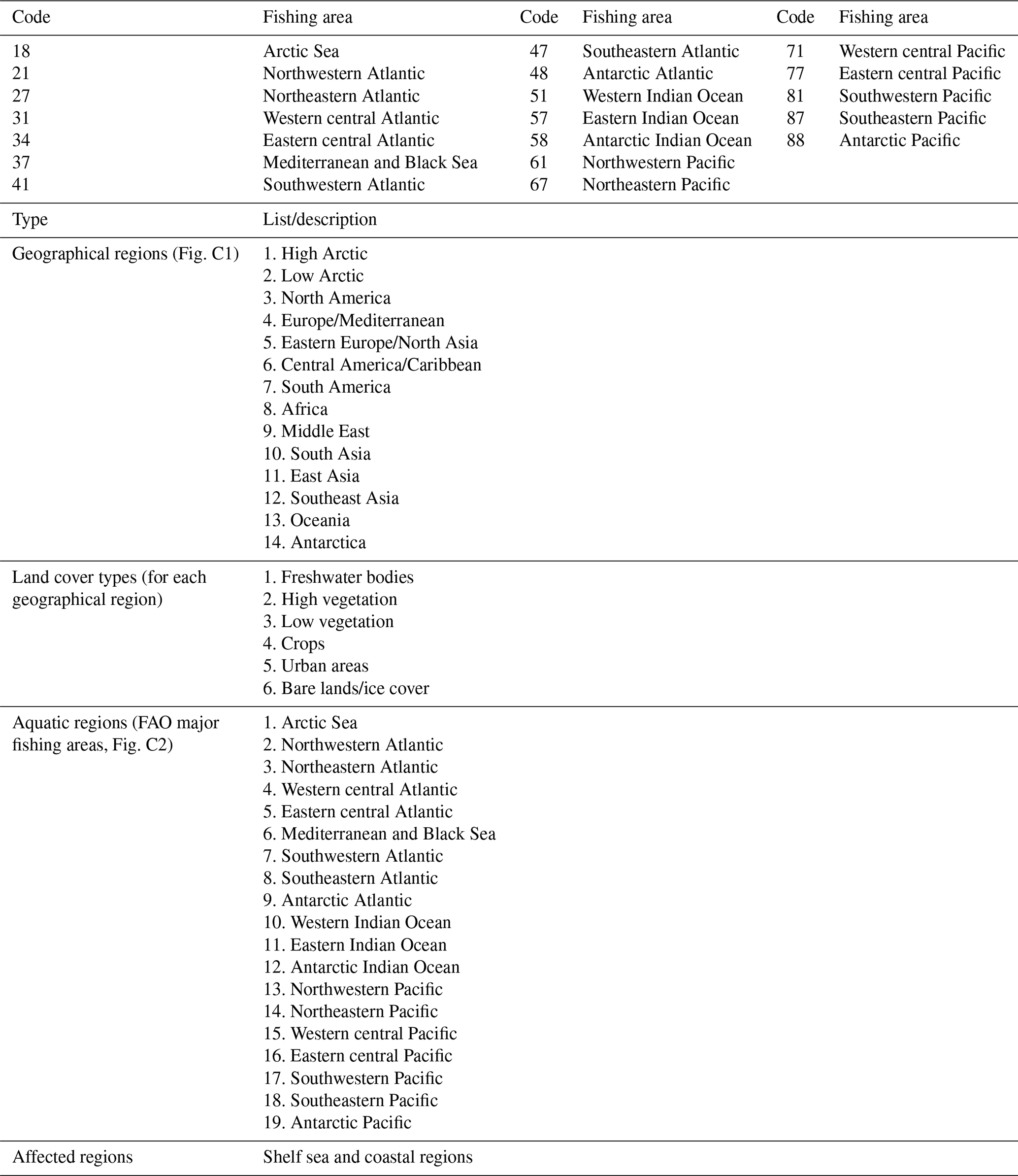
The following formatting rules are required for data submission:
-
All netCDF files should adhere to COARDS conventions. These conventions suggest appropriate attributes (name, units, etc.) for the dimensions of a netCDF file (including time, lev, lat, and long). More details about the requested coordinate dimensions and their metadata can be found in the Supplement Excel spreadsheet detailing the format of output variables (MCHgMAP_atm_output_variables_v4.xlsx). One can use the script isCoards provided by the GEOS-Chem support team to verify whether your file is COARDS-compliant (ignore errors related to _bnds variables or GCHP-specific errors). See here for instructions.
-
netCDF files should be concatenated to reduce the number of files that need to be opened and make I/O more efficient. We have suggested using one file per output variable per month or year, requiring concatenation of individual files. Yearly files are requested for monthly averaged data. Monthly files are requested for daily averaged data and the diurnal-cycle-averaged variables.
-
All netCDF files should be provided with global attributes that describe information about the institution, model experiment, model version and type, contact person, and additional comments. For a full list, see the Excel spreadsheet (MCHgMAP_atm_output_variables_v4.xlsx).
-
All data should be stored in
floatprecision where possible (we do not want to store too much data, sodoubleprecision is unnecessary). -
netCDF files should be deflated (compressed) to reduce their size. This can be done with the command
nccopy -- d1 in_file.nc out_file.nc. -
A README file should be included detailing the data source and contents. It would be helpful to include expected results in this README file, especially for input emission files (i.e., global emission totals for each species or source).
-
Where possible, include scripts used to produce the data. For example, if an input emission file is being submitted, include the script where these emission data are created.
-
Each requested variable (listed in MCHgMAP_atm_output_variables_v4.xlsx in the Supplement) should be provided in a separate file containing all time steps for a year (for monthly averages) or month (for daily or diurnal averages). The files should be constructed according to the convention
mchgmap_<ModelName>_<ExperimentName>_<VariableName>_<VerticalCoordinate Type>_<Period>_<Frequency>.ncwhere: <ModelName> should be chosen so that the model's name, model version, and possibly the institution can be identified. No underscores (_) are allowed in <ModelName>, use hyphens (–) instead. Restrict <ModelName> to a maximum of 20 characters. <ExperimentName> should correspond to the model experiment codes from Tables F8 to F10. <VariableName> should correspond to the output variable short names in the Excel spreadsheet (MCHgMAP_atm_output_variables_v4.xlsx). <VerticalCoordinateType> is the surface or model level from the output spreadsheet. <Period> is the year and/or month of the data, in format YYYY (monthly data) or YYYYMM (daily data). <Frequency> refers to time-invariant, monthly, daily, or diurnal. -
Several variables (related to meteorological data) are only requested for the baseline simulations. A column in MCHgMAP_atm_output_variables_v4.xlsx details whether the variables are necessary for all of the simulations or only the baseline simulation.
E1 Historical anthropogenic emissions
Table E1Overview of the anthropogenic atmospheric Hg emission inventories.
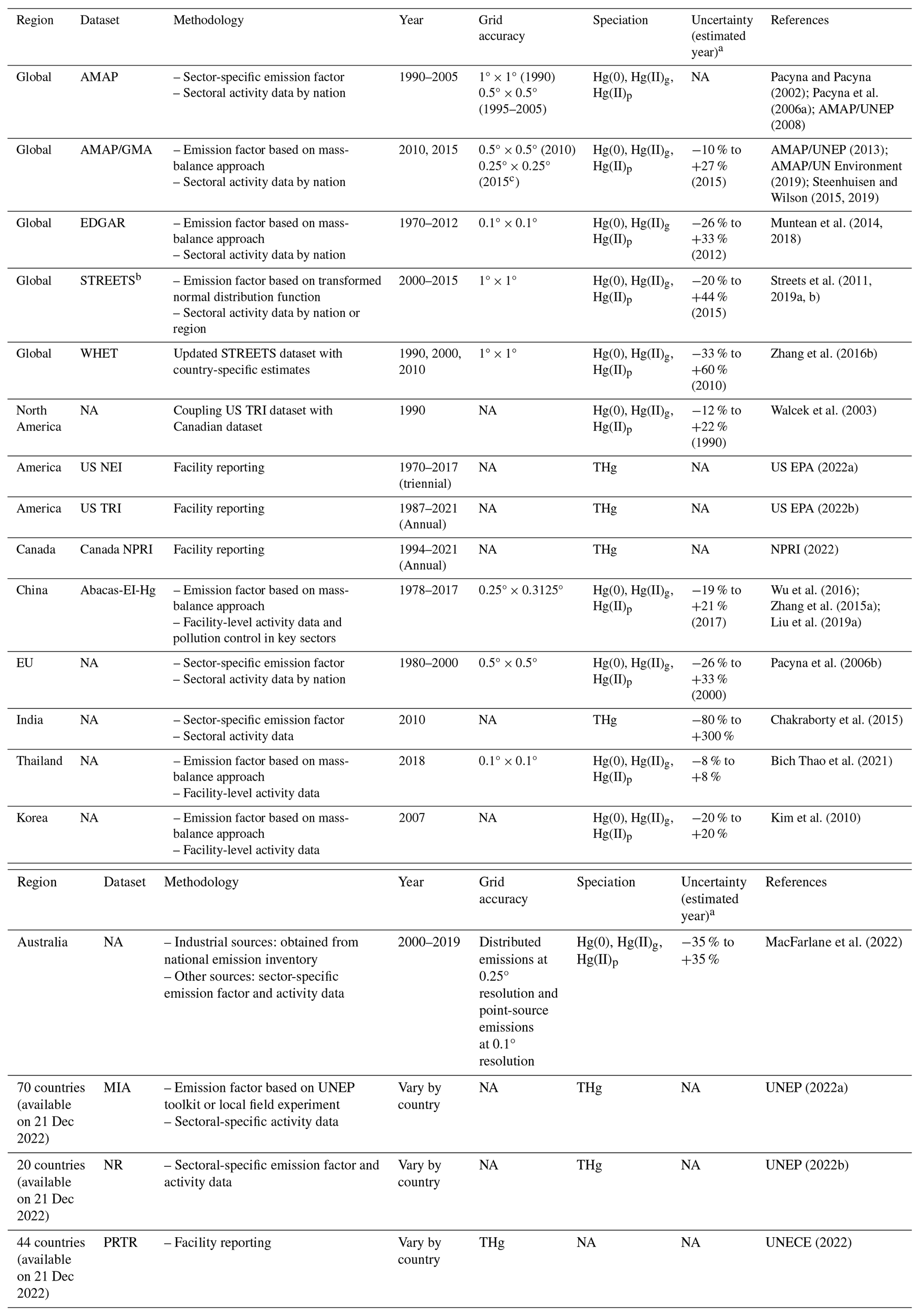
Notes: a If the studied inventory involves emission in multiple years, only the uncertainty range of the latest year is listed in the table. b The Hg emission inventory compiled by Streets et al. (2011, 2019a, b) is referred to as STREETS in this paper. c Also available at 0.1° grid resolution. NA – not available; Hg(0) – gaseous elemental Hg; Hg(II)g – gaseous oxidized Hg; Hg(II)p – particulate-bound Hg; MIA – Hg initial assessment; NR – national report to UNEP; THg – total Hg.
Table E2Sectoral emissions in different global anthropogenic atmospheric Hg emission inventories.
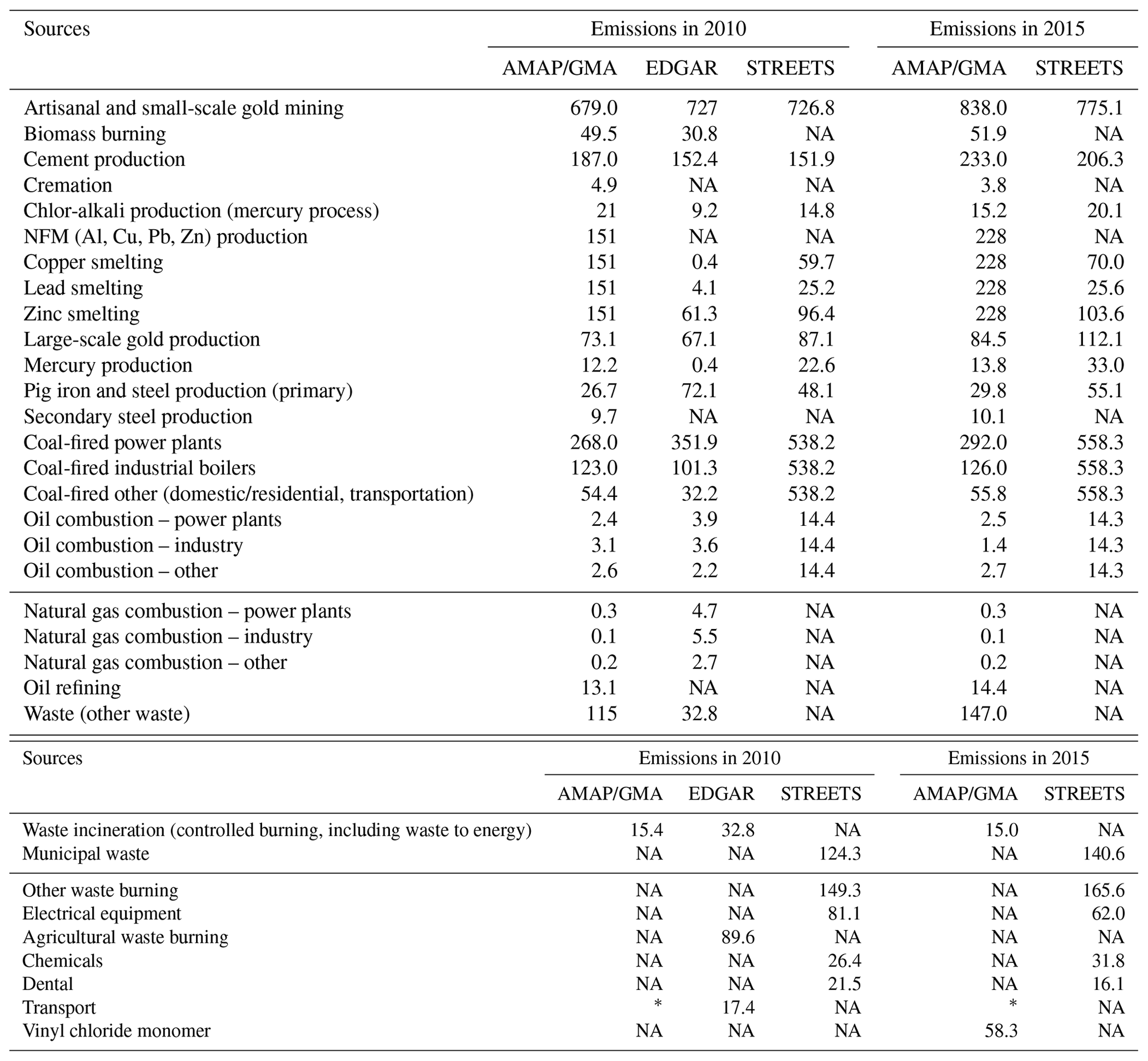
Note: NA – Not available; * – included in coal/oil/gas combustion “other”.
Table E3Spatial point source and proxy rasters applied in different anthropogenic Hg emission inventories. Minamata Convention target sectors are shown in bold.
Notes: 1 In EDGARv4 1970–2012, the mercury emissions from biomass combustion in power generation are distributed using the proxies of coal, gas, oil, and auto-producers7. 2 AMAP_1990 was distributed using the 1990 global population and a limited number of large emission point sources. 3 AMAP 1995–2005 was distributed using an increasing number of point sources over time. The remaining (diffuse) emissions were distributed over several different proxies. A percentage of point source and spatial proxy distribution would only be valid for a specific year and therefore cannot be given for the 1995–2005 period. 4 Percentages for the 2015 emission distribution. 5 AMAP/UN Environnement utilizes point source emission information derived from national emission inventories and from additional (open) sources as described in Steenhuisen and Wilson (2015, 2019). 6 Combustion emissions from fuel use during the manufacture of secondary and tertiary products from solid fuels, including production of charcoal (IPCC, 2006, classification 1.A.1.c). 7 Activities which generate electricity or heat wholly or partly for their own use, as an activity that supports their primary activity (EDGAR 1.A.1.a). When all emissions (100 %) of a given sector are distributed using point source information, no proxy raster has been used. Hence, the proxy raster is listed as NA. Minamata target sectors (in bold): coal-fired power plants; coal-fired industrial boilers; nonferrous metal smelting (zinc, lead, copper, and large-scale gold production); waste incineration; cement clinker production; ASGM; and mercury (primary) production.
Table E4Speciation profile used in the AMAP/GMA, WHET, and EDGAR (%) global Hg emission inventories. Bold is the generic speciation profile.
NA: not available.
E2 Future anthropogenic emissions
Table E6Scenario design for future Hg emissions: considerations and resulting scenarios.
Table E7Data sources and other considerations for building future Hg emission scenarios.
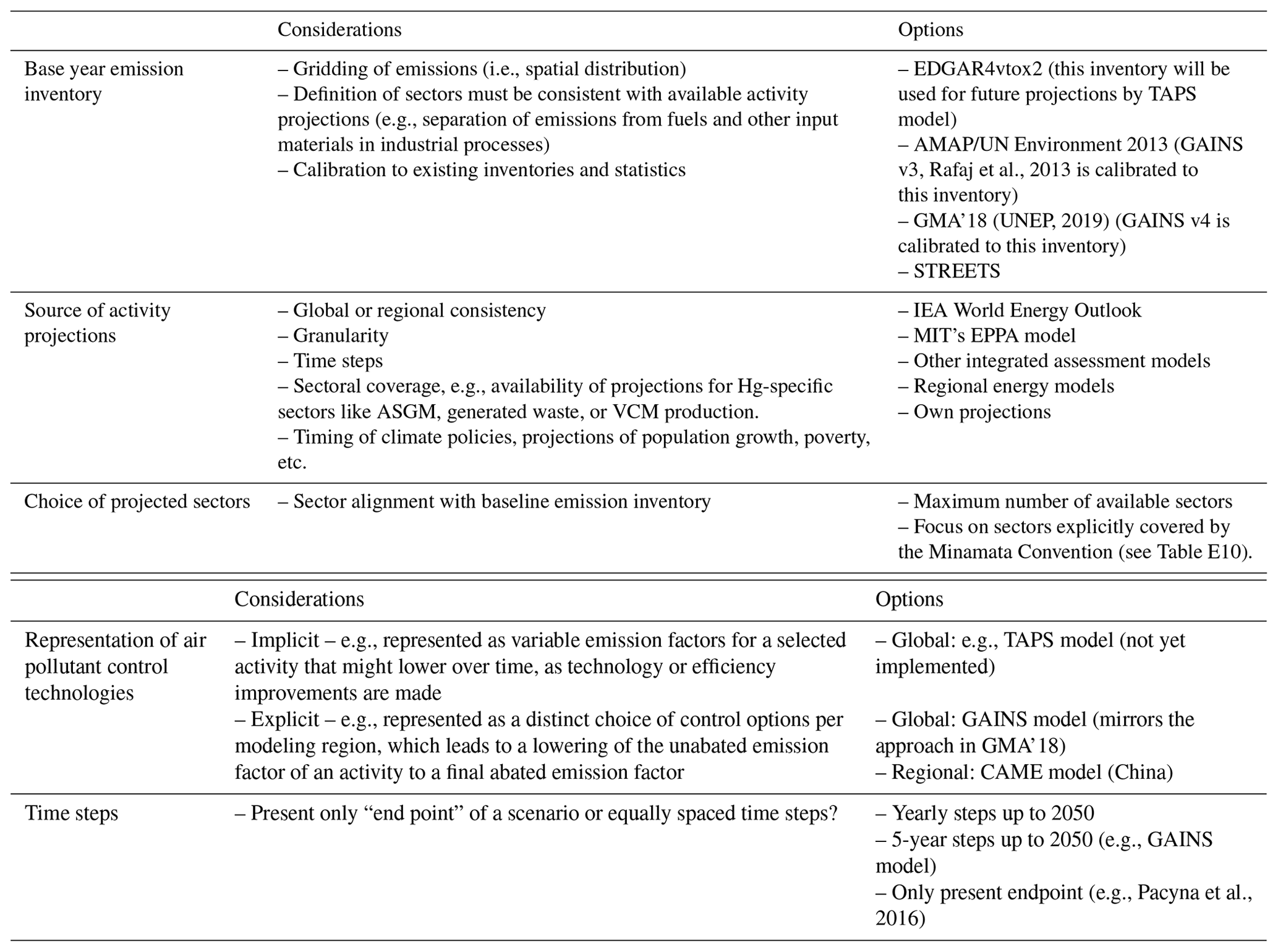
Table E8Global projections of mercury emissions in the literature. BAS – baseline energy or activity scenario; CLIM – climate mitigation scenario for energy and activities; CLE – current legislation for Hg pollution control; MFR – maximum feasible Hg reduction; SRES – Special Report on Emission Scenarios; WEO – World Energy Outlook; ETP – Energy Technology Perspectives.
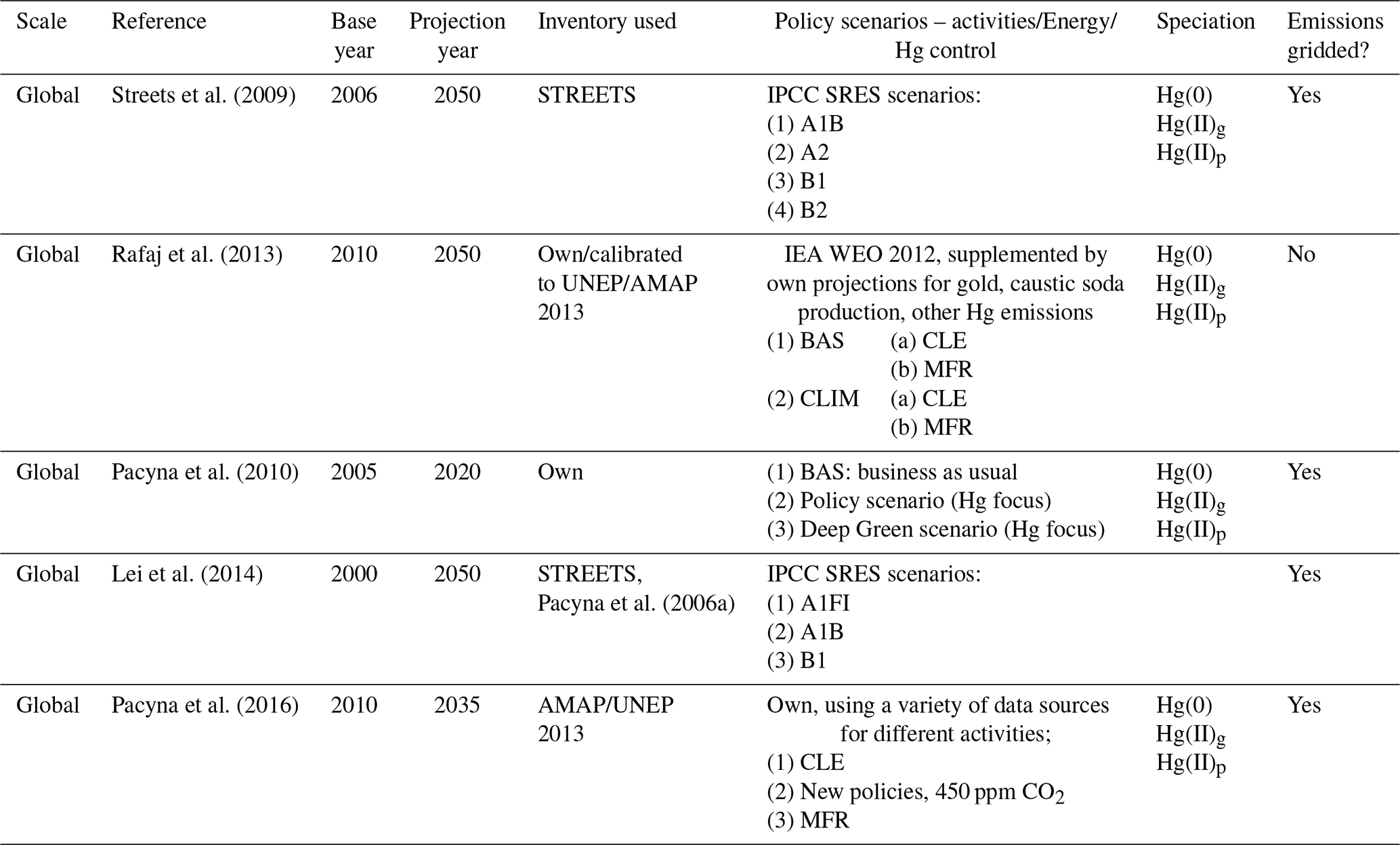
Table E9Regional projections of mercury emissions in the literature. APCD – air pollution control device; BAS – baseline energy or activity scenario; BAU – business-as-usual scenario; CCS – carbon capture and storage; CLIM – climate mitigation scenario for energy and activities; CLE – current legislation for Hg pollution control; HgCD – Hg control device; MFR – maximum feasible Hg reduction; SRES —Special Report on Emission Scenarios; WEO – IEA World Energy Outlook.
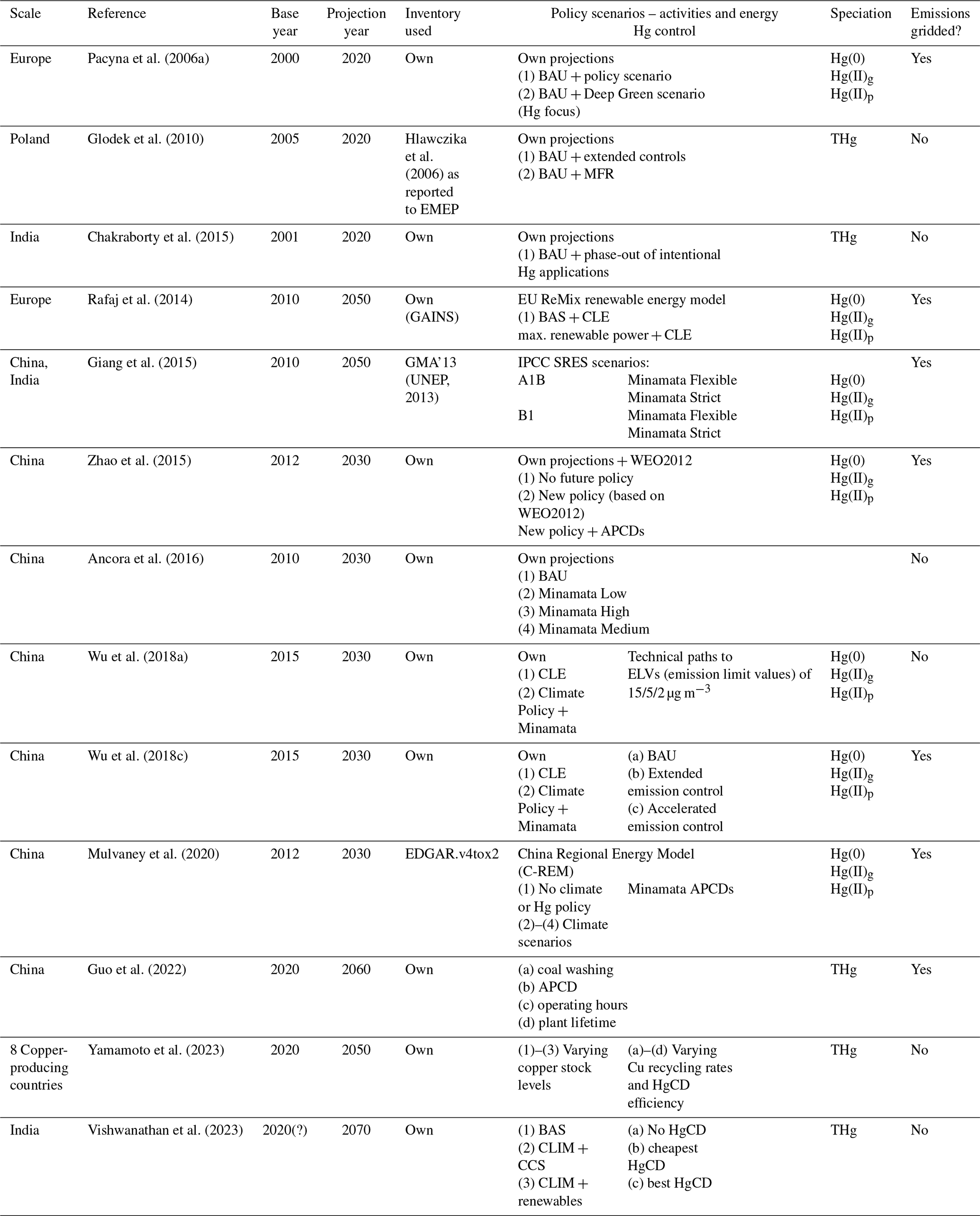
Table E10Anthropogenic emission sectors covered by different future global emission scenario modeling efforts in the literature. ASGM – artisanal and small-scale gold mining; EC – emission control; Red/BAN – reduction or ban; VCM – vinyl chloride monomer production.
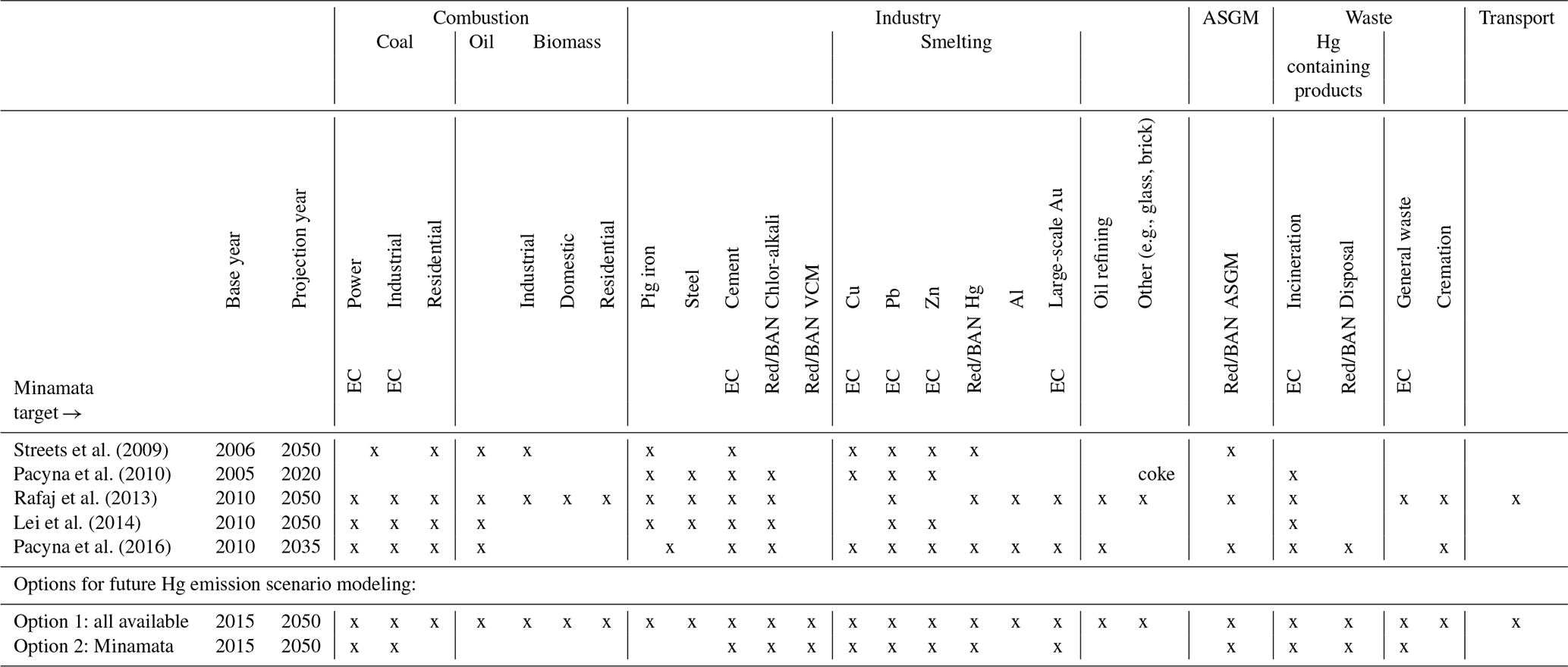
Table E11Proposed setup for GAINS v4 and TAPS future Hg emission scenarios.
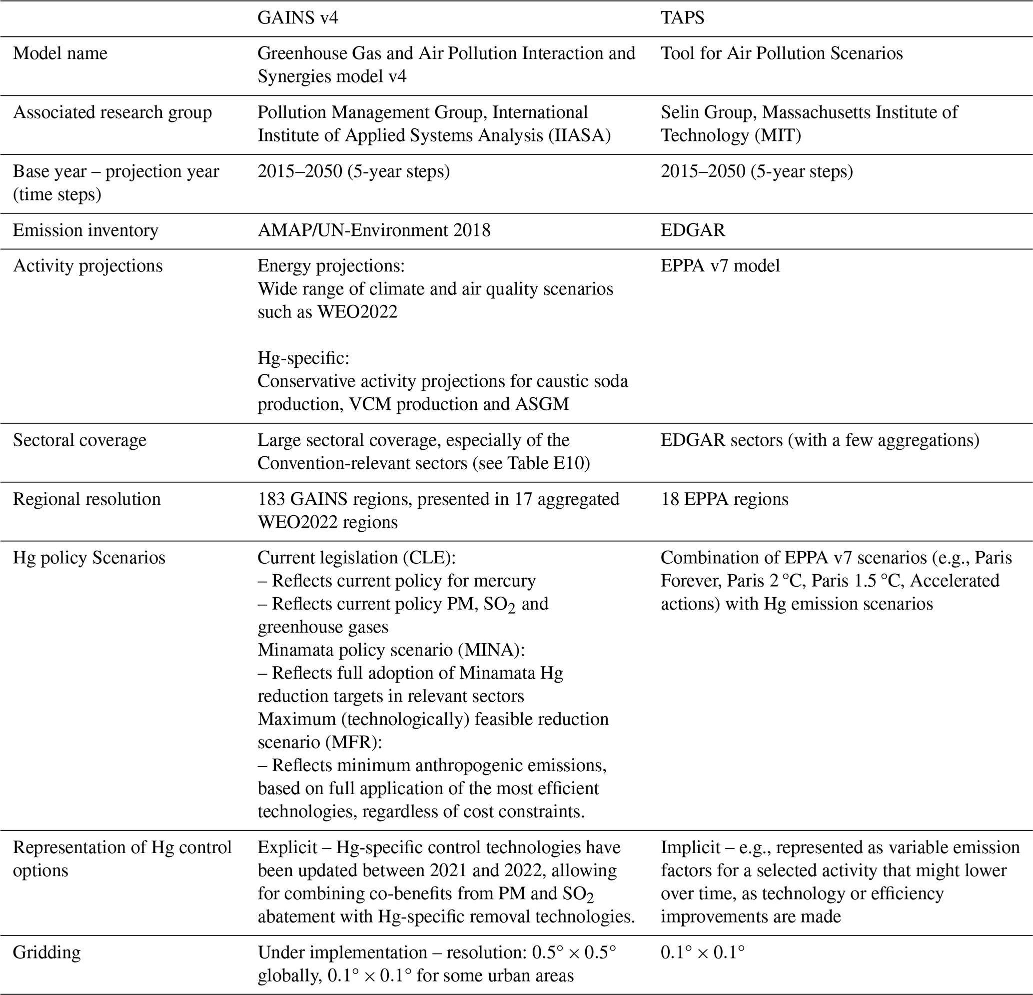
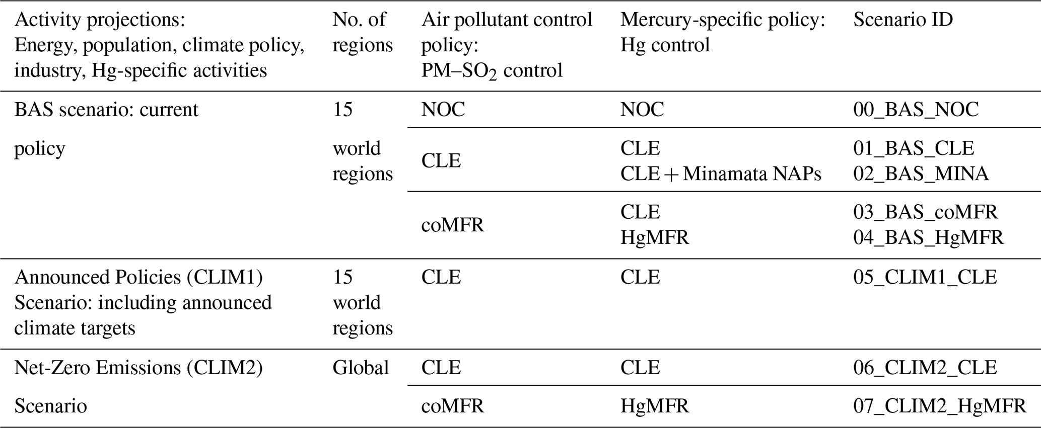
IIASA's GAINS model has been used to evaluate air pollution and greenhouse gas policies for several decades (Amann et al., 2011). As a multi-pollutant model, GAINS includes emission factors and control strategies for SO2, PM, NH3, N2O, NOx, CH4, CO2, CO, VOC, F-gases and Hg from anthropogenic emission sources. Currently, 55 emission sectors are combined with 15 activity types are associated with Hg emission factors, leading to a nuanced description of Hg emissions. The model relies on exogenous activity inputs from integrated assessment models, extended by additional mercury-specific activity inputs. It contains a bottom-up inventory of pollution control options for each pollutant, on the basis of its 182 regions on the global level, which for many regions are coordinated in consultation with local experts. Mercury co-benefits from existing PM and SO2 control are calculated automatically for all applicable combustion and industry sectors and additional mercury control strategies can be added, based on current and future policy. Results are presented in 5-year steps up to 2050.
The following paragraphs describe the most current Hg-GAINS scenarios, for which publication is planned in 2023.
Inventory used and activity projections
The World Energy Outlook scenarios for 2022 are currently implemented in GAINS and have been used as activities for the most recent Hg scenarios. Data on ASGM, caustic soda production, Hg mining, and VCM were derived from the Global Mercury Assessment, USGS mineral yearbooks, and similar sources. ASGM and VCM production are kept constant until 2050, representing a conservative estimate which can be used to illustrate policy changes clearly. The ratio of bodies cremated is kept constant until 2050, but cremation activities are driven by population growth.
Emission factors
Unabated mercury emission factors in GAINS are derived from different literature sources and the Global Mercury Assessment, aggregated (e.g., the nonferrous metal sector) and disaggregated (e.g., the iron and steel sectors) as appropriate to the model resolution. Emission factors for the combustion sectors are documented in Rafaj et al. (2013), and others have been developed based on information in the GMA'18 (Global Mercury Assessment 2018, 2020). Unabated emission factors are constant through all the model years. Specific emission factors were developed for the waste sector. GAINSv4 was calibrated to the 2015 emissions in GMA'18 (highest transparency), and all changes are documented.
Air pollution control policies in GAINS
The global mercury scenarios make use of the most up-to-date PM and SO2 control policies from the recently implemented WEO2022 scenarios, utilizing both the CLE and cost-optimal maximum feasible reduction (MFR) scenarios for PM and SO2 control. Hg co-benefits for the PM–SO2 CLE and MFR are calculated within the model for all types of combustion and industry sectors. Where relevant legislation exists, e.g., in the EU, Hg-specific control options are then added to the co-benefit control strategy. Where a Hg-specific control strategy overlaps with existing PM or SO2, a hierarchy of controls is implemented whereby the most efficient ones are assumed to be implemented in the most technologically advanced installations. Additional Hg-specific controls include, e.g., the EU directive on large combustion plants concerning waste incineration, phase-out of caustic soda production using mercury cells, and all Minamata National Action Plans for ASGM reduction published until December 2022.
Results from the scenarios will be reported following the regional resolution of the IEA World Energy Outlook 2022, which uses 15 world regions: (1) North America excluding the United States; (2) the United States; (3) Central and South America excluding Brazil; (4) Brazil; (5) Europe excluding the European Union; (6) the European Union; (7) Africa excluding South Africa; (8) South Africa; (9) the Middle East; (10) Eurasia; (11) Asia Pacific excluding China, India, Japan, and Southeast Asia; (12) China; (13) India; (14) Japan; and (15) Southeast Asia.
Table F1Three-dimensional global and regional atmospheric Hg models.
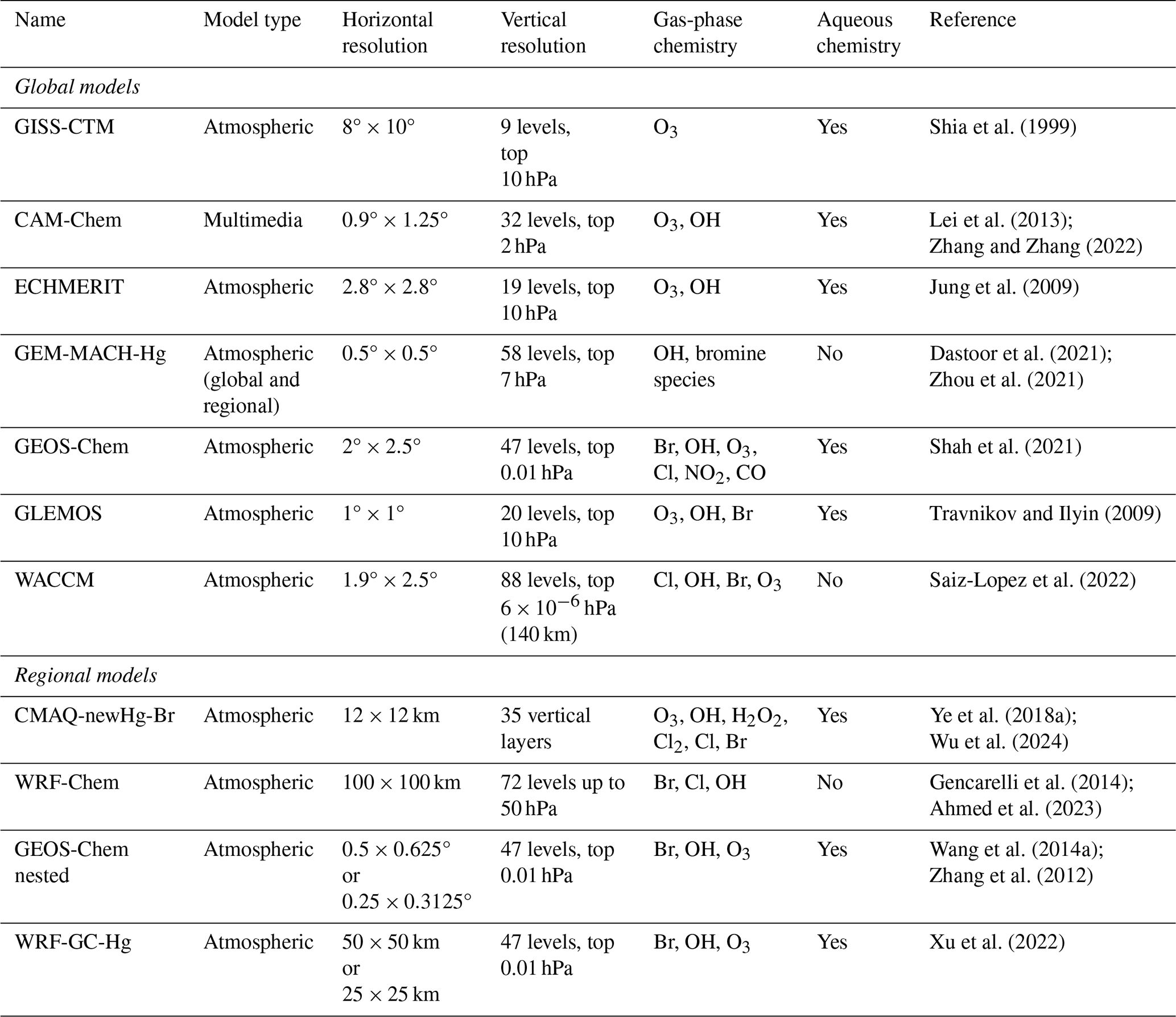
Table F2Three-dimensional global and regional ocean Hg models.
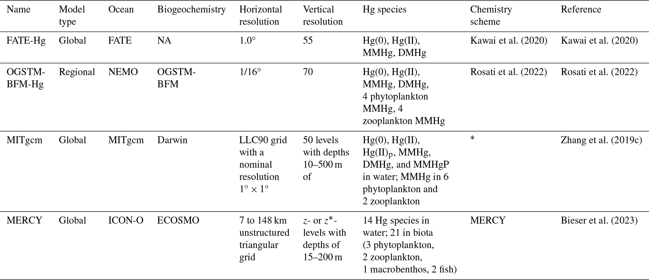
* The inorganic Hg chemistry in MITgcm-Hg includes photochemical and biological redox conversions between dissolved Hg(0) and Hg(II) in the oceanic mixed layer and biologically mediated redox reactions in the subsurface ocean. The dark oxidation of dissolved Hg(0) in the mixed layer is also included. The formation rates of methylated Hg are parameterized according to microbial remineralization of organic carbon. The photochemical and dark demethylation processes are included. The rate constants of photochemical reactions are scaled by the shortwave radiation intensity attenuated by ocean pigments (chlorophyll and dissolved organic carbon). The dark demethylation rate is calculated as a function of seawater temperature. CH3Hg uptake by phytoplankton is simulated with volume concentration factors as a function of cell size and seawater DOC concentration. The trophic transfer of CH3Hg to zooplankton is modeled with the processes including zooplankton grazing, excretion, and mortality. NA is not applicable.
Table F3Multimedia mass balance models. The numbers in parentheses give the number of boxes per media.
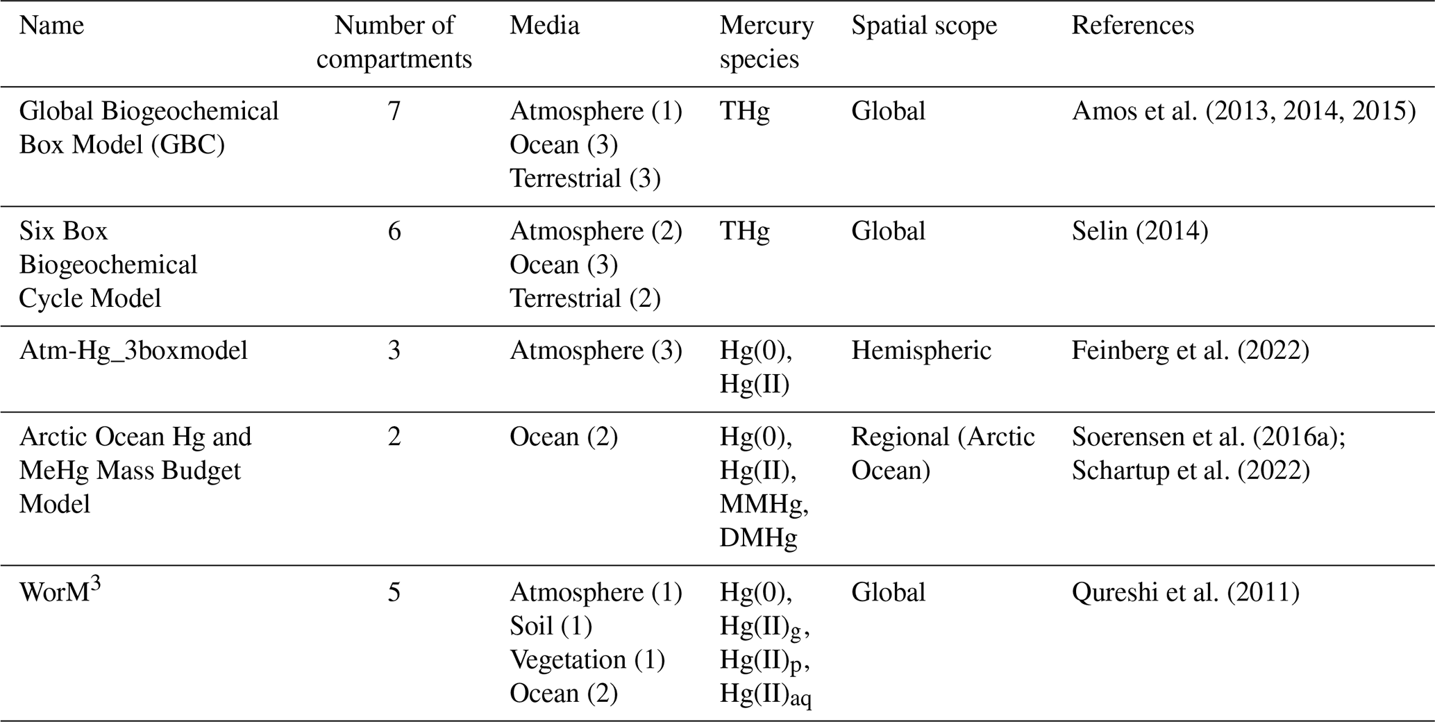
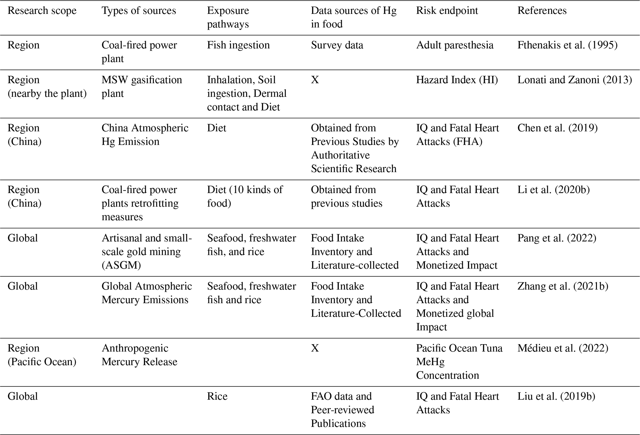
Table F5Global atmospheric model drivers. External and internal atmospheric model drivers. Different options for harmonizing drivers for the multimodel exercise are given in the last column, with the option for the baseline simulation being highlighted in bold.
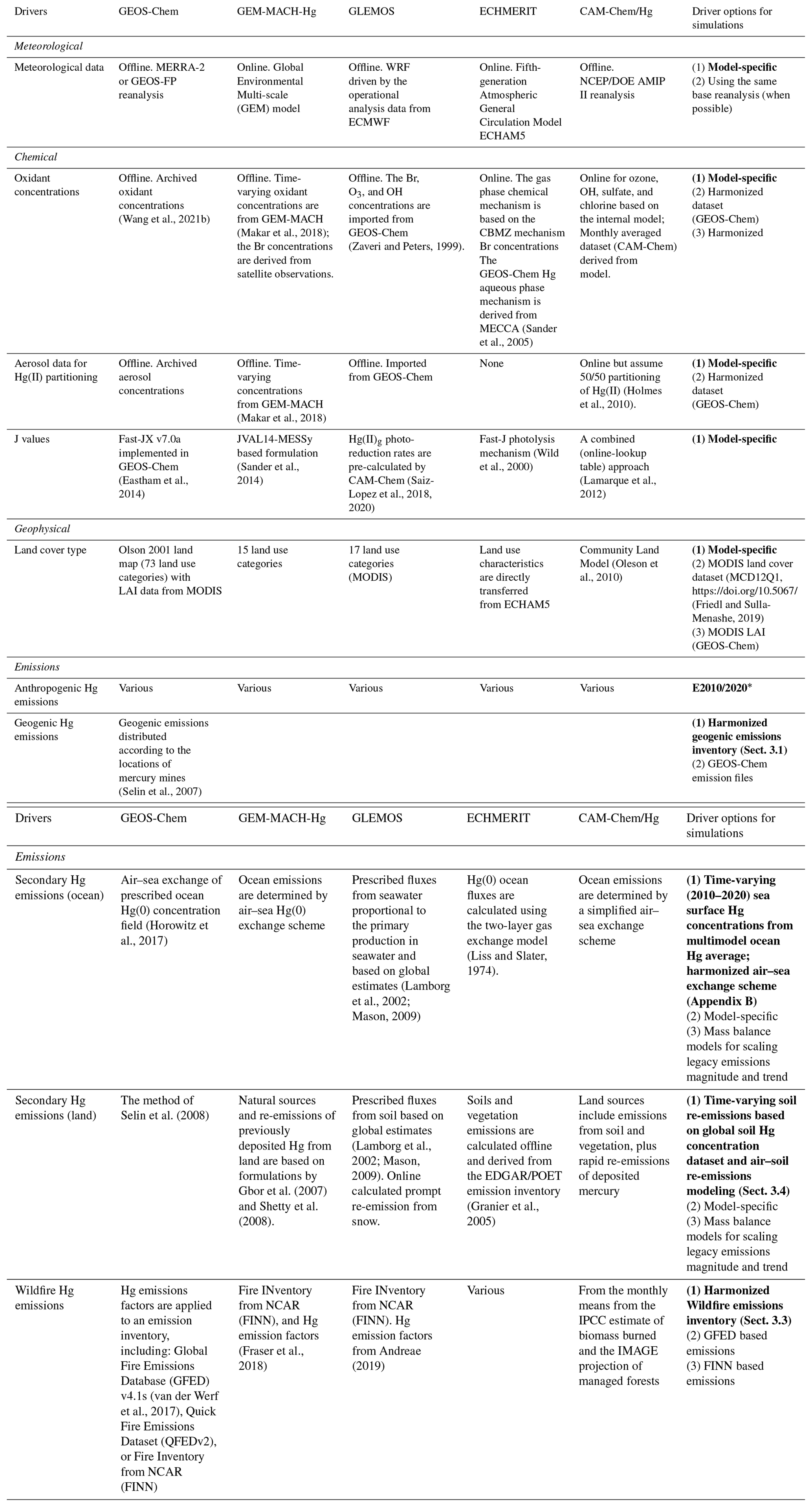
* E2010/2020: Updated spatially distributed global anthropogenic emission inventories from 2010 to 2020 as available for the study (see Sect. 3.2.1).
Table F6Ocean model drivers. External and internal marine model environmental drivers that could be the cause of trends in regional or global ocean Hg concentration during the past and coming decades. References are focused on prior model studies on the impact of these drivers (regional to global context).
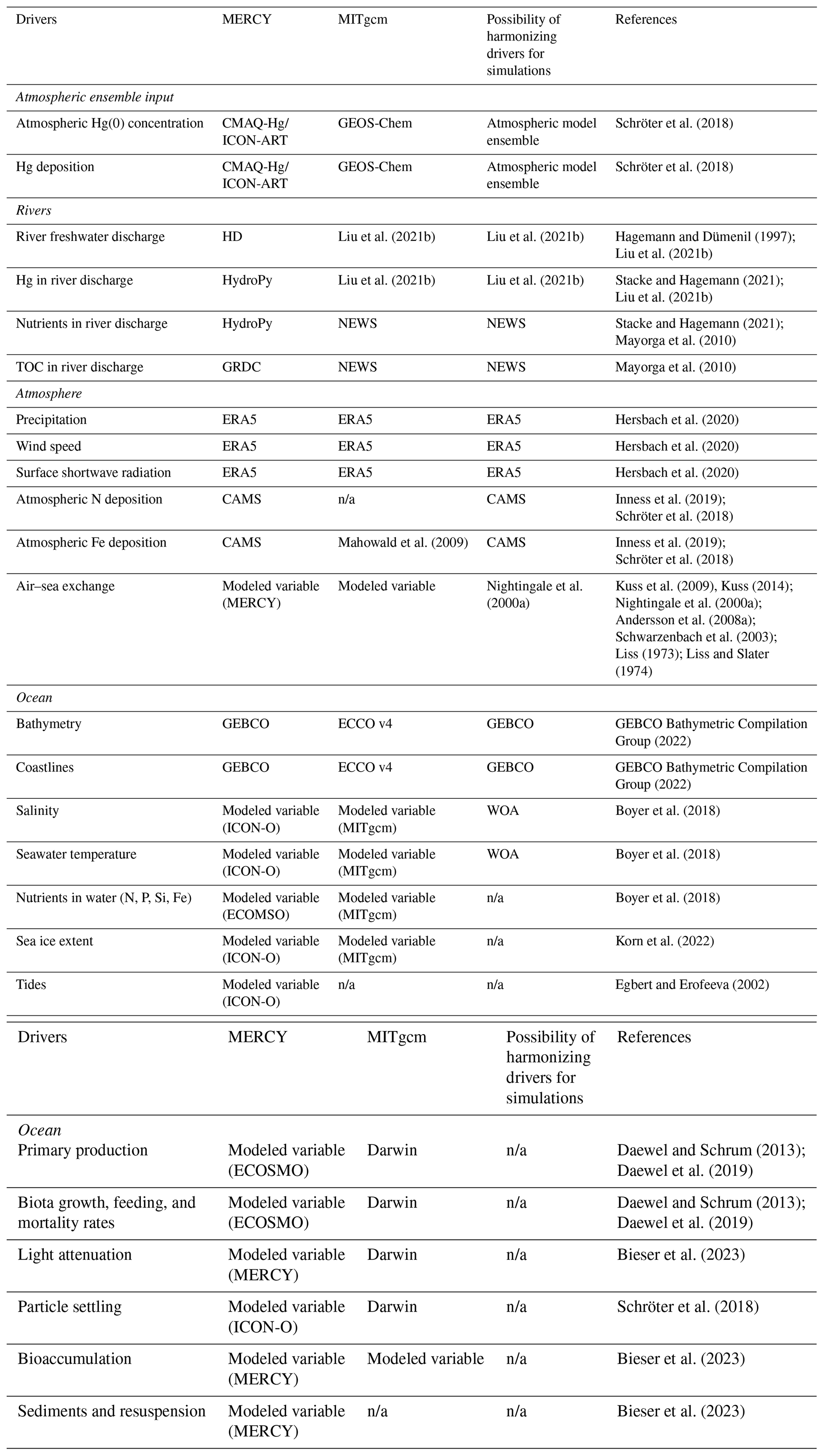
“n/a” stands for not applicable.
Table F8Atmospheric multimodel ensemble simulations.
a Priority ranking: (1) “Core simulations”, expected to be performed by all global models; (2) “Optional simulations”, expected to be performed by as many models as possible; and (3) “Future simulations” to be conducted by a multimodel study following the modeling and analysis study based on retrospective simulations (i.e., priority rankings 1 and 2). b Simulations with the other emission inventories will depend on availability of these inventories at the time of the multimodel project (see Sect. 3.2.1 for discussion of inventories). c Abbreviations: E_mos – Mosaic inventory, i.e., E2010/2020 + available regional emission inventories for the time period. 1 The contribution of a source type to Hg levels is obtained by subtraction of results of the perturbation simulation from results of the baseline simulation (Simulation A1). The contribution of oceanic Hg re-emissions is calculated by subtracting all other source simulations (A2.1–A2.4) from baseline (A1). 2 The contribution of a factor to changes in Hg levels is obtained by subtraction of results of the perturbation simulation from results of the baseline simulation (Simulation A1). 3 The contribution of a factor to future changes in Hg levels is obtained by subtraction of results of the perturbation simulation from results of the future baseline simulation (Simulation A6.1).
Table F9Ocean multimodel ensemble simulations.
a Priority ranking: (1) “Core simulations”, expected to be performed by all global models; (2) “Optional simulations”, expected to be performed by as many models as possible; and (3) “Future simulations” to be conducted by a multimodel study following the modeling and analysis study based on retrospective simulations (i.e., priority rankings 1 and 2). b Abbreviations: E_mos – Mosaic inventory: E2010/2020 + available regional emission inventories for the time period. c Simulations with the other emission inventories will depend on availability of these inventories at the time of the multimodel project (see Sect. 3.2.1 for a discussion of the inventories).
Table F10Mass balance model simulations. All simulations will be performed with the model ensemble (see Sect. 5.3) to account for uncertainties in Hg emissions, rate constants, and fluxes. In addition, all the simulations listed here are “core simulations”.
* All simulations begin from the analytical steady state calculated for model rates + geogenic emissions.
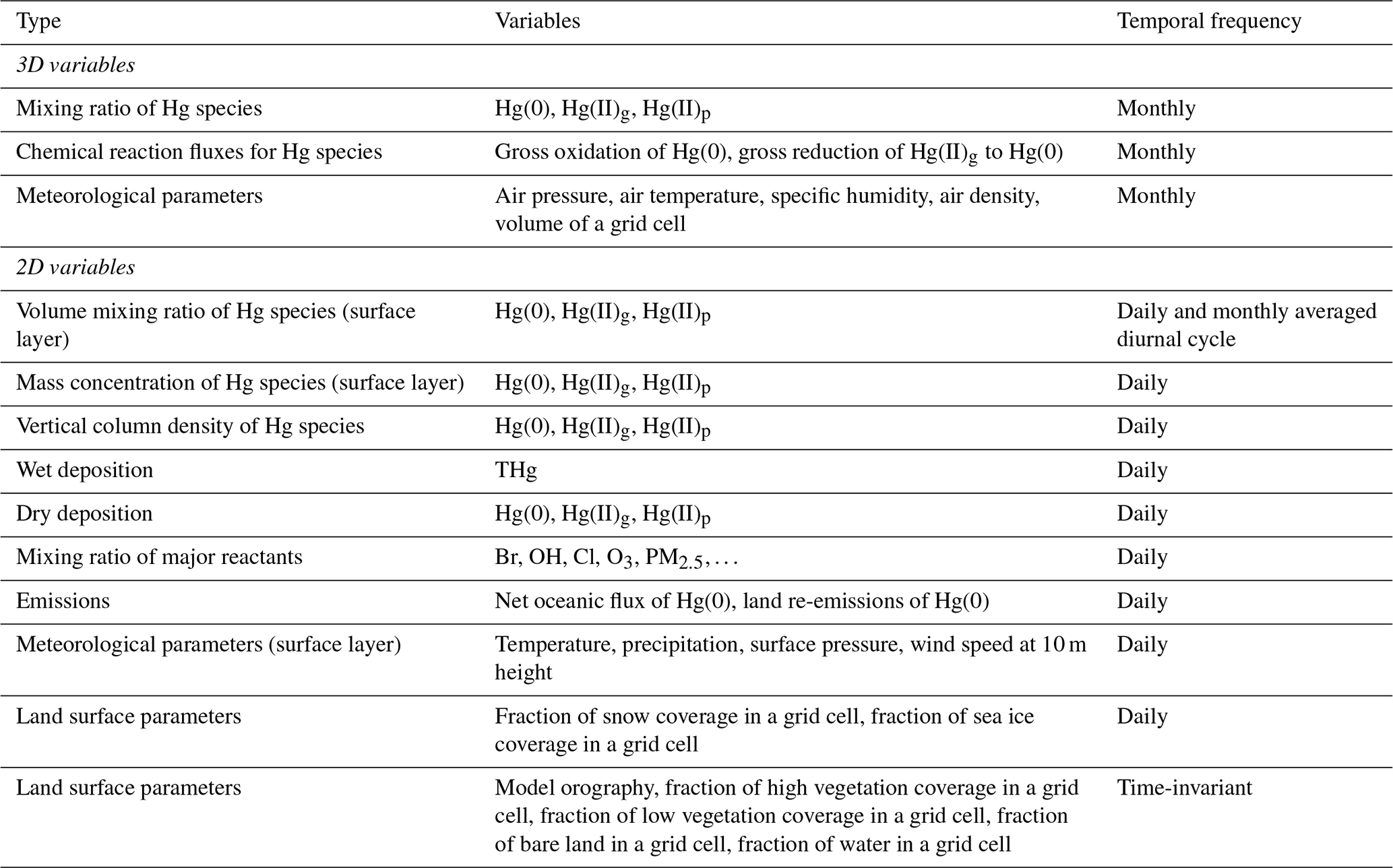
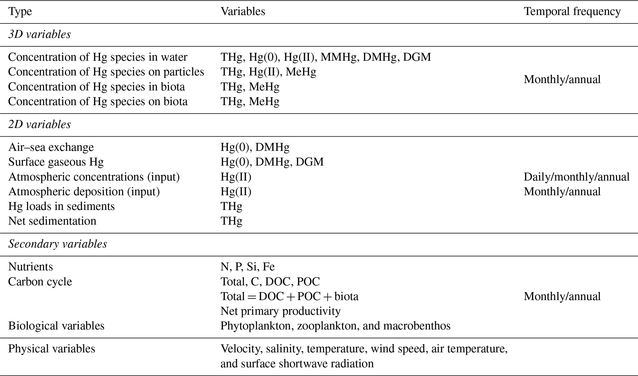
The anthropogenic emission datasets analyzed in this study are available publicly (EDGAR: https://doi.org/10.5281/zenodo.12155169, Muntean et al., 2017; AMAP: https://doi.org/10.34894/F3J91I, Steenhuisen and Wilson, 2024, and https://doi.org/10.34894/SZ2KOI, Steenhuisen and Wilson, 2022; and STREETS: https://doi.org/10.5281/zenodo.11717314, Wu, 2024).
AD led the overall design and development of the study and writing of the article with contributions from all the authors, listed in alphabetical order with the lead authors identified in bold: AD, HA, JB, FB, BE, AF, XF, BG, CG, YH, IMH, II, JK, CJL, IL, RM, DM, MM, PR, EMR, AR, NES, FDS, ALS, FS, OT, SW, XW, SW, RW, QW, YZ, JZ, WZ, and SZ.
The contact author has declared that none of the authors has any competing interests.
Publisher's note: Copernicus Publications remains neutral with regard to jurisdictional claims made in the text, published maps, institutional affiliations, or any other geographical representation in this paper. While Copernicus Publications makes every effort to include appropriate place names, the final responsibility lies with the authors.
We thank Terry Keating, co-chair of the Minamata Convention OESG and the LRTAP Convention TF-HTAP, for organizing the modeling initiative by fostering the dialog with international institutions and contributing to the discussion throughout the development of this work. We thank Jenny Fisher for the review and comments on the manuscript.
Qingru Wu was supported by the National Natural Science Foundation of China (grant nos. 42394094 and 2222604). Aryeh Feinberg was supported by the Swiss National Science Foundation (grant no. P2EZP2_195424), the US National Science Foundation (grant no. 1924148), and Horizon Europe (Marie Skłodowska-Curie grant agreement no. 101103544). Contribution of Oleg Travnikov was funded by the EU GMOS-Train project of the European Union's Horizon 2020 research and innovation program under Marie Sklodowska-Curie grant agreement no. 860497 and co-funded by the ARRS Research Programme P1-0143 and J1-3033 (IsoCont). The views expressed are those of the authors and do not necessarily represent those of their employers or funding agencies.
This paper was edited by Yilong Wang and reviewed by four anonymous referees.
Aas, W. and Bohlin-Nizzetto, P.: Heavy Metals and POP Measurements, NILU, https://nilu.brage.unit.no/nilu-xmlui/handle/11250/2828494 (last access: 1 May 2025), 2019.
Agather, A. M., Bowman, K. L., Lamborg, C. H., and Hammerschmidt, C. R.: Distribution of mercury species in the Western Arctic Ocean (U.S. GEOTRACES GN01), Mar. Chem., 216, 103686, https://doi.org/10.1016/j.marchem.2019.103686, 2019.
Agnan, Y., Le Dantec, T., Moore, C. W., Edwards, G. C., and Obrist, D.: New Constraints on Terrestrial Surface–Atmosphere Fluxes of Gaseous Elemental Mercury Using a Global Database, Environ. Sci. Technol., 50, 507–524, https://doi.org/10.1021/acs.est.5b04013, 2016.
Ahmed, S., Thomas, J. L., Angot, H., Dommergue, A., Archer, S. D., Bariteau, L., Beck, I., Benavent, N., Blechschmidt, A.-M., Blomquist, B., Boyer, M., Christensen, J. H., Dahlke, S., Dastoor, A., Helmig, D., Howard, D., Jacobi, H.-W., Jokinen, T., Lapere, R., Laurila, T., Quéléver, L. L. J., Richter, A., Ryjkov, A., Mahajan, A. S., Marelle, L., Pfaffhuber, K. A., Posman, K., Rinke, A., Saiz-Lopez, A., Schmale, J., Skov, H., Steffen, A., Stupple, G., Stutz, J., Travnikov, O., and Zilker, B.: Modelling the coupled mercury-halogen-ozone cycle in the central Arctic during spring, Elem. Sci. Anthr., 11, 00129, https://doi.org/10.1525/elementa.2022.00129, 2023.
Aiuppa, A., Dongarrà, G., Valenza, M., Federico, C., and Pecoraino, G.: Degassing of Trace Volatile Metals During the 2001 Eruption of Etna, in: Volcanism and the Earth's Atmosphere, AGU – American Geophysical Union, 41–54, https://doi.org/10.1029/139GM03, 2004.
Aiuppa, A., Bagnato, E., Witt, M. L. I., Mather, T. A., Parello, F., Pyle, D. M., and Martin, R. S.: Real-time simultaneous detection of volcanic Hg and SO2 at La Fossa Crater, Vulcano (Aeolian Islands, Sicily), Geophys. Res. Lett., 34, L21307, https://doi.org/10.1029/2007GL030762, 2007.
Amann, M., Bertok, I., Borken-Kleefeld, J., Cofala, J., Heyes, C., Höglund-Isaksson, L., Klimont, Z., Nguyen, B., Posch, M., Rafaj, P., Sandler, R., Schöpp, W., Wagner, F., and Winiwarter, W.: Cost-effective control of air quality and greenhouse gases in Europe: Modeling and policy applications, Environ. Model. Softw., 26, 1489–1501, https://doi.org/10.1016/j.envsoft.2011.07.012, 2011.
AMAP: AMAP Assessment Report: Arctic Pollution Issues, AMAP – Arctic Monitoring and Assessment Programme, Oslo, Norway, https://www.amap.no/documents/doc/amap-assessment-report-arctic-pollution-issues/68 (last access: 1 May 2025), 1998.
AMAP/UN Environnement: Technical Background Report for the Global Mercury Assessment 2018, Arctic Monitoring and Assessment Programme, Oslo, Norway/UN Environnement Programme, Chemicals and Health Branch, Geneva, Switzerland, https://www.amap.no/documents/doc/technical-background-report-for-the-global-mercury-assessment (last access: 1 May 2025), 2019.
AMAP/UNEP: Technical Background Report to the Global Atmospheric Mercury Assessment, Arctic Monitoring and Assessment Programme/UNEP Chemicals Branch, https://www.amap.no/documents/doc/technical-background-report-to-the-global-atmospheric-mercury (last access: 1 May 2025), 2008.
AMAP/UNEP: Technical Background Report for the Global Mercury Assessment 2013, Arctic Monitoring and Assessment Porgramme, Oslo, Norway, UNEP Chemicals Branch, Geneva, Switzerland, https://www.amap.no/documents/doc/technical-background-report-for-the-global-mercury (last access: 1 May 2025), 2013.
Ambrose, J., Tsiros, and Wool: Modeling mercury fluxes and concentrations in a Georgia watershed receiving atmospheric deposition load from direct and indirect sources, J. Air Waste Manage. Assoc., 55, 547–558, https://doi.org/10.1080/10473289.2005.10464643, 2005.
Ammar, Y., Faxneld, S., Sköld, M., and Soerensen, A. L.: Long-term database for contaminants in fish, mussels, and bird eggs from the Baltic Sea, Sci. Data, 11, 400, https://doi.org/10.1038/s41597-024-03216-0, 2024.
Amos, H. M., Jacob, D. J., Streets, D. G., and Sunderland, E. M.: Legacy impacts of all-time anthropogenic emissions on the global mercury cycle, Global Biogeochem. Cy., 27, 410–421, https://doi.org/10.1002/gbc.20040, 2013.
Amos, H. M., Jacob, D. J., Kocman, D., Horowitz, H. M., Zhang, Y., Dutkiewicz, S., Horvat, M., Corbitt, E. S., Krabbenhoft, D. P., and Sunderland, E. M.: Global Biogeochemical Implications of Mercury Discharges from Rivers and Sediment Burial, Environ. Sci. Technol., 48, 9514–9522, https://doi.org/10.1021/es502134t, 2014.
Amos, H. M., Sonke, J. E., Obrist, D., Robins, N., Hagan, N., Horowitz, H. M., Mason, R. P., Witt, M., Hedgecock, I. M., Corbitt, E. S., and Sunderland, E. M.: Observational and Modeling Constraints on Global Anthropogenic Enrichment of Mercury, Environ. Sci. Technol., 49, 4036–4047, https://doi.org/10.1021/es5058665, 2015.
Amptmeijer, D. J. and Bieser, J.: The relevance of feeding strategy on the accumulation of Hg and MMHg, in: Goldschmidt 2023 Conference, Lyon, https://conf.goldschmidt.info/goldschmidt/2023/meetingapp.cgi/Paper/20541 (last access: 1 May 2025), 2023.
Ancora, M. P., Zhang, L., Wang, S., Schreifels, J. J., and Hao, J.: Meeting Minamata: Cost-effective compliance options for atmospheric mercury control in Chinese coal-fired power plants, Energy Policy, 88, 485–494, 2016.
Andersson, M. E., Gårdfeldt, K., Wängberg, I., and Strömberg, D.: Determination of Henry's law constant for elemental mercury, Chemosphere, 73, 587–592, https://doi.org/10.1016/j.chemosphere.2008.05.067, 2008a.
Andersson, M. E., Sommar, J., Gårdfeldt, K., and Lindqvist, O.: Enhanced concentrations of dissolved gaseous mercury in the surface waters of the Arctic Ocean, Mar. Chem., 110, 190–194, https://doi.org/10.1016/j.marchem.2008.04.002, 2008b.
Andreae, M. O.: Emission of trace gases and aerosols from biomass burning – an updated assessment, Atmos. Chem. Phys., 19, 8523–8546, https://doi.org/10.5194/acp-19-8523-2019, 2019.
Angot, H., Dastoor, A., De Simone, F., Gårdfeldt, K., Gencarelli, C. N., Hedgecock, I. M., Langer, S., Magand, O., Mastromonaco, M. N., Nordstrøm, C., Pfaffhuber, K. A., Pirrone, N., Ryjkov, A., Selin, N. E., Skov, H., Song, S., Sprovieri, F., Steffen, A., Toyota, K., Travnikov, O., Yang, X., and Dommergue, A.: Chemical cycling and deposition of atmospheric mercury in polar regions:review of recent measurements and comparison with models, Atmos. Chem. Phys., 16, 10735–10763, https://doi.org/10.5194/acp-16-10735-2016, 2016.
Angot, H., Hoffman, N., Giang, A., Thackray, C. P., Hendricks, A. N., Urban, N. R., and Selin, N. E.: Global and Local Impacts of Delayed Mercury Mitigation Efforts, Environ. Sci. Technol., 52, 12968–12977, https://doi.org/10.1021/acs.est.8b04542, 2018.
Arnold, J., Gustin, M. S., and Weisberg, P. J.: Evidence for Nonstomatal Uptake of Hg by Aspen and Translocation of Hg from Foliage to Tree Rings in Austrian Pine, Environ. Sci. Technol., 52, 1174–1182, https://doi.org/10.1021/acs.est.7b04468, 2018.
Assad, M., Parelle, J., Cazaux, D., Gimbert, F., Chalot, M., and Tatin-Froux, F.: Mercury uptake into poplar leaves, Chemosphere, 146, 1–7, https://doi.org/10.1016/j.chemosphere.2015.11.103, 2016.
Atkinson, W., Eastham, S. D., Chen, Y.-H. H., Morris, J., Paltsev, S., Schlosser, C. A., and Selin, N. E.: A tool for air pollution scenarios (TAPS v1.0) to enable global, long-term, and flexible study of climate and air quality policies, Geosci. Model Dev., 15, 7767–7789, https://doi.org/10.5194/gmd-15-7767-2022, 2022.
Back, S.-K., Mojammal, A. H. M., Kim, J.-H., Kim, Y.-H., Seok, K.-S., and Seo, Y.-C.: Mercury distribution analyses and estimation of recoverable mercury amount from byproducts in primary metal production facilities using UNEP toolkit and on-site measurement, J. Mater. Cycl. Waste Manage., 21, 915–924, https://doi.org/10.1007/s10163-019-00851-3, 2019.
Bagnato, E., Aiuppa, A., Parello, F., Calabrese, S., D'Alessandro, W., Mather, T. A., McGonigle, A. J. S., Pyle, D. M., and Wängberg, I.: Degassing of gaseous (elemental and reactive) and particulate mercury from Mount Etna volcano (Southern Italy), Atmos. Environ., 41, 7377–7388, https://doi.org/10.1016/j.atmosenv.2007.05.060, 2007.
Bagnato, E., Parello, F., Valenza, M., and Caliro, S.: Mercury content and speciation in the Phlegrean Fields volcanic complex: Evidence from hydrothermal system and fumaroles, J. Volcanol. Geoth. Res., 187, 250–260, https://doi.org/10.1016/j.jvolgeores.2009.09.010, 2009.
Bagnato, E., Aiuppa, A., Parello, F., Allard, P., Shinohara, H., Liuzzo, M., and Giudice, G.: New clues on the contribution of Earth's volcanism to the global mercury cycle, Bull. Volcanol., 73, 497–510, https://doi.org/10.1007/s00445-010-0419-y, 2011.
Bagnato, E., Tamburello, G., Aiuppa, A., Sprovieri, M., Vougioukalakis, G. E., and Parks, M.: Mercury emissions from soils and fumaroles of Nea Kameni volcanic centre, Santorini (Greece), Geochem. J., 47, 437–450, https://doi.org/10.2343/geochemj.2.0263, 2013.
Bagnato, E., Barra, M., Cardellini, C., Chiodini, G., Parello, F., and Sprovieri, M.: First combined flux chamber survey of mercury and CO2 emissions from soil diffuse degassing at Solfatara of Pozzuoli crater, Campi Flegrei (Italy): Mapping and quantification of gas release, J. Volcanol. Geoth. Res., 289, 26–40, https://doi.org/10.1016/j.jvolgeores.2014.10.017, 2014.
Bagnato, E., Tamburello, G., Avard, G., Martinez-Cruz, M., Enrico, M., Fu, X., Sprovieri, M., and Sonke, J. E.: Mercury fluxes from volcanic and geothermal sources: an update, Geol. Soc. Lond. Spec. Publ., 410, 263–285, https://doi.org/10.1144/SP410.2, 2015.
Bagnato, E., Viveiros, F., Pacheco, J. E., D'Agostino, F., Silva, C., and Zanon, V.: Hg and CO2 emissions from soil diffuse degassing and fumaroles at Furnas Volcano (São Miguel Island, Azores): Gas flux and thermal energy output, J. Geochem. Explor., 190, 39–57, https://doi.org/10.1016/j.gexplo.2018.02.017, 2018.
Ballabio, C., Jiskra, M., Osterwalder, S., Borrelli, P., Montanarella, L., and Panagos, P.: A spatial assessment of mercury content in the European Union topsoil, Sci. Total Environ., 769, 144755, https://doi.org/10.1016/j.scitotenv.2020.144755, 2021.
Bash, J. O.: Description and initial simulation of a dynamic bidirectional air-surface exchange model for mercury in Community Multiscale Air Quality (CMAQ) model, J. Geophys. Res.-Atmos., 115, D0635, https://doi.org/10.1029/2009JD012834, 2010.
Bash, J. O., Miller, D. R., Meyer, T. H., and Bresnahan, P. A.: Northeast United States and Southeast Canada natural mercury emissions estimated with a surface emission model, Atmos. Environ., 38, 5683–5692, 2004.
Beal, S., Osterberg, E. C., Zdanowicz, C., and Fisher, D.: An ice core perspective on mercury pollution during the past 600 years, Environ. Sci. Technol., 49, 7641–7647, 2015.
Bebout, D. C.: Mercury: Inorganic & Coordination Chemistry, in: Encyclopedia of Inorganic Chemistry, John Wiley & Sons, Ltd, https://doi.org/10.1002/0470862106.ia131, 2006.
Becnel, J., Falgeust, C., Cavalier, T., Gauthreaux, K., Landry, F., Blanchard, M., Beck, M. J., and Beck, J. N.: Correlation of mercury concentrations in tree core and lichen samples in southeastern Louisiana, Microchem. J., 78, 205–210, https://doi.org/10.1016/j.microc.2004.06.002, 2004.
Bich Thao, P. T., Pimonsree, S., Suppoung, K., Bonnet, S., Junpen, A., and Garivait, S.: Development of an anthropogenic atmospheric mercury emissions inventory in Thailand in 2018, Atmos. Pollut. Res., 12, 101170, https://doi.org/10.1016/j.apr.2021.101170, 2021.
Bieser, J. and Schrum, C.: Impact of marine mercury cycling on coastal atmospheric mercury concentrations in the North- and Baltic Sea region, Elem. Sci. Anthr., 4, 000111, https://doi.org/10.12952/journal.elementa.000111, 2016.
Bieser, J., Simone, F. D., Gencarelli, C., Geyer, B., Hedgecock, I., Matthias, V., Travnikov, O., and Weigelt, A.: A diagnostic evaluation of modeled mercury wet depositions in Europe using atmospheric speciated high-resolution observations, Environ. Sci. Pollut. Res., 21, 9995–10012, https://doi.org/10.1007/s11356-014-2863-2, 2014.
Bieser, J., Slemr, F., Ambrose, J., Brenninkmeijer, C., Brooks, S., Dastoor, A., DeSimone, F., Ebinghaus, R., Gencarelli, C. N., Geyer, B., Gratz, L. E., Hedgecock, I. M., Jaffe, D., Kelley, P., Lin, C.-J., Jaegle, L., Matthias, V., Ryjkov, A., Selin, N. E., Song, S., Travnikov, O., Weigelt, A., Luke, W., Ren, X., Zahn, A., Yang, X., Zhu, Y., and Pirrone, N.: Multi-model study of mercury dispersion in the atmosphere: vertical and interhemispheric distribution of mercury species, Atmos. Chem. Phys., 17, 6925–6955, https://doi.org/10.5194/acp-17-6925-2017, 2017.
Bieser, J., Amptmeijer, D. J., Daewel, U., Kuss, J., Soerensen, A. L., and Schrum, C.: The 3D biogeochemical marine mercury cycling model MERCY v2.0 – linking atmospheric Hg to methylmercury in fish, Geosci. Model Dev., 16, 2649–2688, https://doi.org/10.5194/gmd-16-2649-2023, 2023.
Biester, H. and Scholz, C.: Determination of Mercury Binding Forms in Contaminated Soils: Mercury Pyrolysis versus Sequential Extractions, Environ. Sci. Technol., 31, 233–239, https://doi.org/10.1021/es960369h, 1997.
Biester, H., Pérez-Rodríguez, M., Gilfedder, B.-S., Martínez Cortizas, A., and Hermanns, Y.-M.: Solar irradiance and primary productivity controlled mercury accumulation in sediments of a remote lake in the Southern Hemisphere during the past 4000 years, Limnol. Oceanogr., 63, 540–549, https://doi.org/10.1002/lno.10647, 2018.
Bindler, R.: Estimating the natural background atmospheric deposition rate of mercury utilizing ombrotrophic bogs in southern Sweden, Environ. Sci. Technol., 37, 40–46, https://doi.org/10.1021/es020065x, 2003.
Bishop, K., Shanley, J. B., Riscassi, A., de Wit, H. A., Eklöf, K., Meng, B., Mitchell, C., Osterwalder, S., Schuster, P. F., Webster, J., Zhu, W.: Recent advances in understanding and measurement of mercury in the environment: Terrestrial Hg cycling, Sci. Total Environ., 721, 137647, https://doi.org/10.1016/j.scitotenv.2020.137647, 2020.
Biswas, A., Blum, J. D., Klaue, B., and Keeler, G. J.: Release of mercury from Rocky Mountain forest fires, Global Biogeochem. Cy., 21, GB1002, https://doi.org/10.1029/2006GB002696, 2007.
Biswas, A., Blum, J. D., Bergquist, B. A., Keeler, G. J., and Xie, Z.: Natural Mercury Isotope Variation in Coal Deposits and Organic Soils, Environ. Sci. Technol., 42, 8303–8309, https://doi.org/10.1021/es801444b, 2008.
Blackwell, B. D. and Driscoll, C. T.: Using foliar and forest floor mercury concentrations to assess spatial patterns of mercury deposition, Environ. Pollut., 202, 126–134, https://doi.org/10.1016/j.envpol.2015.02.036, 2015.
Blais, J. M., Kalff, J., Cornett, R. J., and Evans, R. D.: Evaluation of 210Pb dating in lake sediments using stable Pb, Ambrosia pollen, and 137Cs, J. Paleolimnol., 13, 169–178, https://doi.org/10.1007/BF00678105, 1995.
Bousquet, P., Ringeval, B., Pison, I., Dlugokencky, E. J., Brunke, E.-G., Carouge, C., Chevallier, F., Fortems-Cheiney, A., Frankenberg, C., Hauglustaine, D. A., Krummel, P. B., Langenfelds, R. L., Ramonet, M., Schmidt, M., Steele, L. P., Szopa, S., Yver, C., Viovy, N., and Ciais, P.: Source attribution of the changes in atmospheric methane for 2006–2008, Atmos. Chem. Phys., 11, 3689–3700, https://doi.org/10.5194/acp-11-3689-2011, 2011.
Bowdalo, D. R., Evans, M. J., and Sofen, E. D.: Spectral analysis of atmospheric composition: application to surface ozone model–measurement comparisons, Atmos. Chem. Phys., 16, 8295–8308, https://doi.org/10.5194/acp-16-8295-2016, 2016.
Bowman, K. L., Hammerschmidt, C. R., Lamborg, C. H., and Swarr, G.: Mercury in the North Atlantic Ocean: The U.S. GEOTRACES zonal and meridional sections, Deep-Sea Res. Pt. II, 116, 251–261, https://doi.org/10.1016/j.dsr2.2014.07.004, 2015.
Bowman, K. L., Hammerschmidt, C. R., Lamborg, C. H., Swarr, G. J., and Agather, A. M.: Distribution of mercury species across a zonal section of the eastern tropical South Pacific Ocean (U.S. GEOTRACES GP16), Mar. Chem., 186, 156–166, https://doi.org/10.1016/j.marchem.2016.09.005, 2016.
Bowman, K. L., Lamborg, C. H., and Agather, A. M.: A global perspective on mercury cycling in the ocean, Sci. Total Environ., 710, 136166, https://doi.org/10.1016/j.scitotenv.2019.136166, 2019.
Bowman, K. L., Lamborg, C. H., and Agather, A. M.: A global perspective on mercury cycling in the ocean, Sci. Total Environ., 710, 136166, https://doi.org/10.1016/j.scitotenv.2019.136166, 2020.
Box, J. E., Colgan, W. T., Christensen, T. R., Schmidt, N. M., Lund, M., Parmentier, F.-J. W., Brown, R., Bhatt, U. S., Euskirchen, E. S., Romanovsky, V. E., Walsh, J. E., Overland, J. E., Wang, M., Corell, R. W., Meier, W. N., Wouters, B., Mernild, S., Mård, J., Pawlak, J., and Olsen, M. S.: Key indicators of Arctic climate change: 1971–2017, Environ. Res. Lett., 14, 045010, https://doi.org/10.1088/1748-9326/aafc1b, 2019.
Boyer, T. P., García, H. E., Locarnini, R. A., Zweng, M. M., Mishonov, A. V., Reagan, J. R., Weathers, K. A., Baranova, O. K., Paver, C. R., Seidov, D., and Smolyar, I. V.: World Ocean Atlas 2018, NOAA National Centers for Environmental Information [data set], https://www.ncei.noaa.gov/archive/accession/NCEI-WOA18 (last access: 1 May 2025), 2018.
Bratkič, A., Vahèiè, M., Kotnik, J., Obu, V. K., Begu, E., Woodward, E., Malcolm, S., and Horvat, M.: Mercury presence and speciation in the South Atlantic Ocean along the 40° S transect, Global Biogeochem. Cy., 30, 105–119, https://doi.org/10.1002/2015GB005275, 2016.
Bridge, M.: Tree Rings and Climate by H. C. Fritts, Blackburn Press, Caldwell, 567 pp., ISBN 1930665393, 2001.
Brocza, F. M., Rafaj, P., Sander, R., Wagner, F., and Jones, J. M.: Global scenarios of anthropogenic mercury emissions, Atmos. Chem. Phys., 24, 7385–7404, https://doi.org/10.5194/acp-24-7385-2024, 2024.
Bruggeman, J. and Bolding, K.: A general framework for aquatic biogeochemical models, Environ. Model. Softw., 61, 249–265, https://doi.org/10.1016/j.envsoft.2014.04.002, 2014.
Brunke, E.-G. and Labuschagne, C.: Gaseous mercury emissions from a fire in the Cape peninsula, south africa, during january 2000, Geophys. Res. Lett., 28, 1483–1486, 2001.
Bullock, O. R. and Brehme, K. A.: Atmospheric mercury simulation using the CMAQ model: formulation description and analysis of wet deposition results, Atmos. Environ., 36, 2135–2146, https://doi.org/10.1016/S1352-2310(02)00220-0, 2002.
Burger Chakraborty, L., Qureshi, A., Vadenbo, C., and Hellweg, S.: Anthropogenic mercury flows in India and impacts of emission controls, Environ. Sci. Technol., 47, 8105–8113, https://doi.org/10.1021/es401006k, 2013.
Cabassi, J., Venturi, S., Di Bennardo, F., Nisi, B., Tassi, F., Magi, F., Ricci, A., Picchi, G., and Vaselli, O.: Flux measurements of gaseous elemental mercury (GEM) from the geothermal area of “Le Biancane” natural park (Monterotondo Marittimo, Grosseto, Italy): Biogeochemical processes controlling GEM emission, J. Geochem. Explor., 228, 106824, https://doi.org/10.1016/j.gexplo.2021.106824, 2021.
Campeau, A., Eklöf, K., Soerensen, A. L., Åkerblom, S., Yuan, S., Hintelmann, H., Bieroza, M., Köhler, S., and Zdanowicz, C.: Sources of riverine mercury across the Mackenzie River Basin; inferences from a combined HgC isotopes and optical properties approach, Sci. Total Environ., 806, 150808, https://doi.org/10.1016/j.scitotenv.2021.150808, 2022.
Carn, S. A., Fioletov, V. E., McLinden, C. A., Li, C., and Krotkov, N. A.: A decade of global volcanic SO2 emissions measured from space, Sci. Rep., 7, 44095, https://doi.org/10.1038/srep44095, 2017.
Carnevale, C., Finzi, G., Pederzoli, A., Pisoni, E., Thunis, P., Turrini, E., and Volta, M.: Applying the delta tool to support the Air Quality Directive: evaluation of the TCAM chemical transport model, Air Qual. Atmos. Health, 7, 335–346, https://doi.org/10.1007/s11869-014-0240-4, 2014.
Carpi, A. and Lindberg, S. E.: Sunlight-mediated emission of elemental mercury from soil amended with municipal sewage sludge, Environ. Sci. Technol., 31, 2085–2091, 1997.
Caruso, B. S., Cox, T. J., Runkel, R. L., Velleux, M. L., Bencala, K. E., Nordstrom, D. K., Julien, P. Y., Butler, B. A., Alpers, C. N., Marion, A., and Smith, K. S.: Metals fate and transport modelling in streams and watersheds: state of the science and USEPA workshop review, Hydrol. Process., 22, 4011–4021, https://doi.org/10.1002/hyp.7114, 2008.
Castro, M. and Moore, C.: Importance of Gaseous Elemental Mercury Fluxes in Western Maryland, Atmosphere, 7, 110, https://doi.org/10.3390/atmos7090110, 2016.
Castro, P. J., Kellö, V., Cernušák, I., and Dibble, T. S.: Together, Not Separately, OH and O3 Oxidize Hg(0) to Hg(II) in the Atmosphere, J. Phys. Chem. A, 126, 8266–8279, https://doi.org/10.1021/acs.jpca.2c04364, 2022.
Cesário, R., O'Driscoll, N. J., Justino, S., Wilson, C. E., Monteiro, C. E., Zilhão, H., and Canário, J.: Air Concentrations of Gaseous Elemental Mercury and Vegetation–Air Fluxes within Saltmarshes of the Tagus Estuary, Portugal, Atmosphere, 12, 228, https://doi.org/10.3390/atmos12020228, 2021.
Chakraborty, P., Sarkar, A., Vudamala, K., Naik, R., and Nath, B. N.: Organic Matter – A Key Factor in Controlling Mercury Distribution in Estuarine Sediment, Mar. Chem., 173, 302–309, https://doi.org/10.1016/j.marchem.2014.10.005, 2015.
Chang, K.-L., Schultz, M. G., Lan, X., McClure-Begley, A., Petropavlovskikh, I., Xu, X., and Ziemke, J. R.: Trend detection of atmospheric time series: Incorporating appropriate uncertainty estimates and handling extreme events, Elem. Sci. Anthr., 9, 00035, https://doi.org/10.1525/elementa.2021.00035, 2021.
Chang, K.-L., Schultz, M. G., Koren, G., and Selke, N.: Guidance note on best statistical practices for TOAR analyses, arXiv [preprint], https://doi.org/10.48550/arXiv.2304.14236, 2023.
Chellman, N., McConnell, J. R., Arienzo, M., Pederson, G. T., Aarons, S. M., and Csank, A.: Reassessment of the Upper Fremont Glacier Ice-Core Chronologies by Synchronizing of Ice-Core-Water Isotopes to a Nearby Tree-Ring Chronology, Environ. Sci. Technol., 51, 4230–4238, https://doi.org/10.1021/acs.est.6b06574, 2017.
Chen, H. S., Wang, Z. F., Li, J., Tang, X., Ge, B. Z., Wu, X. L., Wild, O., and Carmichael, G. R.: GNAQPMS-Hg v1.0, a global nested atmospheric mercury transport model: model description, evaluation and application to trans-boundary transport of Chinese anthropogenic emissions, Geosci. Model Dev., 8, 2857–2876, https://doi.org/10.5194/gmd-8-2857-2015, 2015.
Chen, L., Wang, H. H., Liu, J. F., Tong, Y. D., Ou, L. B., Zhang, W., Hu, D., Chen, C., and Wang, X. J.: Intercontinental transport and deposition patterns of atmospheric mercury from anthropogenic emissions, Atmos. Chem. Phys., 14, 10163–10176, https://doi.org/10.5194/acp-14-10163-2014, 2014.
Chen, L., Zhang, W., Zhang, Y., Tong, Y., Liu, M., Wang, H., Xie, H., and Wang, X.: Historical and future trends in global source-receptor relationships of mercury, Sci. Total Environ., 610, 24–31, https://doi.org/10.1016/j.scitotenv.2017.07.182, 2018.
Chen, L., Liang, S., Liu, M., Yi, Y., Mi, Z., Zhang, Y., Li, Y., Qi, J., Meng, J., Tang, X., Zhang, H., Tong, Y., Zhang, W., Wang, X., Shu, J., and Yang, Z.: Trans-provincial health impacts of atmospheric mercury emissions in China, Nat. Commun., 10, 1484, https://doi.org/10.1038/s41467-019-09080-6, 2019.
Chen, Y.-H. H., Paltsev, S., Gurgel, A., Reilly, J. M., and Morris, J.: A Multisectoral Dynamic Model for Energy, Economic, and Climate Scenario Analysis, Low Carbon Econ., 13, 70–111, https://doi.org/10.4236/lce.2022.132005, 2022.
Chételat, J., McKinney, M. A., Amyot, M., Dastoor, A., Douglas, T. A., Heimbürger-Boavida, L.-E., Kirk, J., Kahilainen, K. K., Outridge, P. M., Pelletier, N., Skov, H., St. Pierre, K., Vuorenmaa, J., and Wang, F.: Climate change and mercury in the Arctic: Abiotic interactions, Sci. Total Environ., 824, 153715, https://doi.org/10.1016/j.scitotenv.2022.153715, 2022.
Chiarantini, L., Rimondi, V., Benvenuti, M., Beutel, M. W., Costagliola, P., Gonnelli, C., Lattanzi, P., and Paolieri, M.: Black pine (Pinus nigra) barks as biomonitors of airborne mercury pollution, Sci. Total Environ., 569–570, 105–113, https://doi.org/10.1016/j.scitotenv.2016.06.029, 2016.
Ci, Z., Peng, F., Xue, X., and Zhang, X.: Air–surface exchange of gaseous mercury over permafrost soil: an investigation at a high-altitude (4700 m a.s.l.) and remote site in the central Qinghai–Tibet Plateau, Atmos. Chem. Phys., 16, 14741–14754, https://doi.org/10.5194/acp-16-14741-2016, 2016a.
Ci, Z., Zhang, X., Yin, Y., Chen, J., and Wang, S.: Mercury Redox Chemistry in Waters of the Eastern Asian Seas: From Polluted Coast to Clean Open Ocean, Environ. Sci. Technol., 50, 2371–2380, https://doi.org/10.1021/acs.est.5b05372, 2016b.
Cinnirella, S. and Pirrone, N.: Spatial and temporal distributions of mercury emissions from forest fires in Mediterranean region and Russian federation, Atmos. Environ., 40, 7346–7361, https://doi.org/10.1016/j.atmosenv.2006.06.051, 2006.
Cizdziel, J. V., Jiang, Y., Nallamothu, D., Brewer, J. S., and Gao, Z.: Air/Surface Exchange of Gaseous Elemental Mercury at Different Landscapes in Mississippi, USA, Atmosphere, 10, 538, https://doi.org/10.3390/atmos10090538, 2019.
Clackett, S., Porter, T., and Lehnherr, I.: A 400-year record of atmospheric mercury from tree-rings in northwestern Canada, Environ. Sci. Technol., 52, 9625–9633, https://doi.org/10.1021/acs.est.8b01824, 2018.
Clackett, S. P., Porter, T. J., and Lehnherr, I.: The tree-ring mercury record of Klondike gold mining at Bear Creek, central Yukon, Environ. Pollut., 268, 115777, https://doi.org/10.1016/j.envpol.2020.115777, 2021.
Clarke, H., Gibson, R., Cirulis, B., Bradstock, R. A., and Penman, T. D.: Developing and testing models of the drivers of anthropogenic and lightning-caused wildfire ignitions in south-eastern Australia, J. Environ. Manage., 235, 34–41, https://doi.org/10.1016/j.jenvman.2019.01.055, 2019.
Cohen, M. D., Draxler, R. R., Artz, R. S., Blanchard, P., Gustin, M. S., Han, Y.-J., Holsen, T. M., Jaffe, D. A., Kelley, P., Lei, H., Loughner, C. P., Luke, W. T., Lyman, S. N., Niemi, D., Pacyna, J. M., Pilote, M., Poissant, L., Ratte, D., Ren, X., Steenhuisen, F., Steffen, A., Tordon, R., and Wilson, S. J.: Modeling the global atmospheric transport and deposition of mercury to the Great Lakes, Elementa, 4, 000118, https://doi.org/10.12952/journal.elementa.000118, 2016.
Cole, A. S., Steffen, A., Pfaffhuber, K. A., Berg, T., Pilote, M., Poissant, L., Tordon, R., and Hung, H.: Ten-year trends of atmospheric mercury in the high Arctic compared to Canadian sub-Arctic and mid-latitude sites, Atmos. Chem. Phys., 13, 1535–1545, https://doi.org/10.5194/acp-13-1535-2013, 2013.
Cole, A. S., Steffen, A., Eckley, C. S., Narayan, J., Pilote, M., Tordon, R., Graydon, J. A., St. Louis, V. L., Xu, X., and Branfireun, B. A.: A survey of mercury in air and precipitation across Canada: patterns and trends, Atmosphere, 5, 635–668, 2014.
Cooke, C. A., Martínez-Cortizas, A., Bindler, R., and Sexauer Gustin, M.: Environmental archives of atmospheric Hg deposition – A review, Sci. Total Environ., 709, 134800, https://doi.org/10.1016/j.scitotenv.2019.134800, 2020.
Corbitt, E. S., Jacob, D. J., Holmes, C. D., Streets, D. G., and Sunderland, E. M.: Global Source–Receptor Relationships for Mercury Deposition Under Present-Day and 2050 Emissions Scenarios, Environ. Sci. Technol., 45, 10477–10484, https://doi.org/10.1021/es202496y, 2011.
Cossa, D., Coquery, M., Gobeil, C., and Martin, J.-M.: Mercury Fluxes at the Ocean Margins, in: Global and Regional Mercury Cycles: Sources, Fluxes and Mass Balances, edited by: Baeyens, W., Ebinghaus, R., and Vasiliev, O., Springer Netherlands, Dordrecht, 229–247, https://doi.org/10.1007/978-94-009-1780-4_11, 1996.
Cossa, D., Heimbürger, L.-E., Pérez, F. F., García-Ibáñez, M. I., Sonke, J. E., Planquette, H., Lherminier, P., Boutorh, J., Cheize, M., Menzel Barraqueta, J. L., Shelley, R., and Sarthou, G.: Mercury distribution and transport in the North Atlantic Ocean along the GEOTRACES-GA01 transect, Biogeosciences, 15, 2309–2323, https://doi.org/10.5194/bg-15-2309-2018, 2018.
Cossa, D., Knoery, J., Bãnaru, D., Harmelin-Vivien, M., Sonke, J. E., Hedgecock, I. M., Bravo, A. G., Rosati, G., Canu, D., Horvat, M., Sprovieri, F., Pirrone, N., and Heimbürger-Boavida, L.-E.: Mediterranean Mercury Assessment 2022: An Updated Budget, Health Consequences, and Research Perspectives, Environ. Sci. Technol., 56, 3840–3862, https://doi.org/10.1021/acs.est.1c03044, 2022.
Custódio, D., Pfaffhuber, K. A., Spain, T. G., Pankratov, F. F., Strigunova, I., Molepo, K., Skov, H., Bieser, J., and Ebinghaus, R.: Odds and ends of atmospheric mercury in Europe and over the North Atlantic Ocean: temporal trends of 25 years of measurements, Atmos. Chem. Phys., 22, 3827–3840, https://doi.org/10.5194/acp-22-3827-2022, 2022.
Daewel, U. and Schrum, C.: Simulating long-term dynamics of the coupled North Sea and Baltic Sea ecosystem with ECOSMO II: Model description and validation, J. Mar. Syst., 119–120, 30–49, https://doi.org/10.1016/j.jmarsys.2013.03.008, 2013.
Daewel, U., Schrum, C., and Macdonald, J. I.: Towards end-to-end (E2E) modelling in a consistent NPZD-F modelling framework (ECOSMO E2E_v1.0): application to the North Sea and Baltic Sea, Geosci. Model Dev., 12, 1765–1789, https://doi.org/10.5194/gmd-12-1765-2019, 2019.
Dai, M. Q., Geyman, B. M., Hu, X. C., Thackray, C. P., and Sunderland, E. M.: Sociodemographic Disparities in Mercury Exposure from United States Coal-Fired Power Plants, Environ. Sci. Technol. Lett., 10, 589–595, https://doi.org/10.1021/acs.estlett.3c00216, 2023.
Dastoor, A., Ryzhkov, A., Durnford, D., Lehnherr, I., Steffen, A., and Morrison, H.: Atmospheric mercury in the Canadian Arctic. Part II: Insight from modeling, Sci. Total Environ., 509–510, 16–27, https://doi.org/10.1016/j.scitotenv.2014.10.112, 2015.
Dastoor, A., Ryjkov, A., Kos, G., Zhang, J., Kirk, J., Parsons, M., and Steffen, A.: Impact of Athabasca oil sands operations on mercury levels in air and deposition, Atmos. Chem. Phys., 21, 12783–12807, https://doi.org/10.5194/acp-21-12783-2021, 2021.
Dastoor, A., Angot, H., Bieser, J., Christensen, J. H., Douglas, T. A., Heimbürger-Boavida, L.-E., Jiskra, M., Mason, R. P., McLagan, D. S., Obrist, D., Outridge, P. M., Petrova, M. V., Ryjkov, A., St. Pierre, K. A., Schartup, A. T., Soerensen, A. L., Toyota, K., Travnikov, O., Wilson, S. J., and Zdanowicz, C.: Arctic mercury cycling, Nat. Rev. Earth Environ., 3, 589–595, https://doi.org/10.1038/s43017-022-00269-w, 2022a.
Dastoor, A., Wilson, S. J., Travnikov, O., Ryjkov, A., Angot, H., Christensen, J. H., Steenhuisen, F., and Muntean, M.: Arctic atmospheric mercury: Sources and changes, Sci. Total Environ., 839, 156213, https://doi.org/10.1016/j.scitotenv.2022.156213, 2022b.
Dastoor, A. P. and Larocque, Y.: Global circulation of atmospheric mercury: a modelling study, Atmos. Environ., 38, 147–161, 2004.
Davis, E., Lee, D., and O'Brien, K.: CF Conventions for netCDF, ESS Open Arch., https://www.authorea.com/users/524106/articles/595394-cf-conventions-for-netcdf (last access: 1 May 2025), 2020.
DeBano, L. F.: The role of fire and soil heating on water repellency in wildland environments: a review, J. Hydrol., 231–232, 195–206, https://doi.org/10.1016/S0022-1694(00)00194-3, 2000.
Dedeurwaerder, H., Decadt, G., and Baeyens, W.: Estimations of mercury fluxes emitted by Mount Etna Volcano, Bull. Volcanol., 45, 191–196, https://doi.org/10.1007/BF02597729, 1982.
de Groot, W. J., Flannigan, M. D., and Cantin, A. S.: Climate change impacts on future boreal fire regimes, Forest Ecol. Manage., 294, 35–44, https://doi.org/10.1016/j.foreco.2012.09.027, 2013.
Demers, J. D., Blum, J. D., and Zak, D. R.: Mercury isotopes in a forested ecosystem: Implications for air-surface exchange dynamics and the global mercury cycle, Global Biogeochem. Cy., 27, 222–238, https://doi.org/10.1002/gbc.20021, 2013.
Denkenberger, J. S., Driscoll, C. T., Branfireun, B. A., Eckley, C. S., Cohen, M., and Selvendiran, P.: A synthesis of rates and controls on elemental mercury evasion in the Great Lakes Basin, Environ. Pollut., 161, 291–298, https://doi.org/10.1016/j.envpol.2011.06.007, 2012.
Denzler, B., Bogdal, C., Henne, S., Obrist, D., Steinbacher, M., and Hungerbühler, K.: Inversion Approach to Validate Mercury Emissions Based on Background Air Monitoring at the High Altitude Research Station Jungfraujoch (3580 m), Environ. Sci. Technol., 51, 2846–2853, https://doi.org/10.1021/acs.est.6b05630, 2017.
De Simone, F., Gencarelli, C. N., Hedgecock, I. M., and Pirrone, N.: A Modeling Comparison of Mercury Deposition from current Anthropogenic Mercury Emission Inventories, Environ. Sci. Technol., 50, 5154–5162, https://doi.org/10.1021/acs.est.6b00691, 2016.
De Simone, F., Hedgecock, I. M., Carbone, F., Cinnirella, S., Sprovieri, F., and Pirrone, N.: Estimating Uncertainty in Global Mercury Emission Source and Deposition Receptor Relationships, Atmosphere, 8, 236, https://doi.org/10.3390/atmos8120236, 2017a.
De Simone, F., Artaxo, P., Bencardino, M., Cinnirella, S., Carbone, F., D'Amore, F., Dommergue, A., Feng, X. B., Gencarelli, C. N., Hedgecock, I. M., Landis, M. S., Sprovieri, F., Suzuki, N., Wängberg, I., and Pirrone, N.: Particulate-phase mercury emissions from biomass burning and impact on resulting deposition: a modelling assessment, Atmos. Chem. Phys., 17, 1881–1899, https://doi.org/10.5194/acp-17-1881-2017, 2017b.
De Simone, F., D'Amore, F., Marasco, F., Carbone, F., Bencardino, M., Hedgecock, I. M., Cinnirella, S., Sprovieri, F., and Pirrone, N.: A Chemical Transport Model Emulator for the Interactive Evaluation of Mercury Emission Reduction Scenarios, Atmosphere, 11, 878, https://doi.org/10.3390/atmos11080878, 2020.
De Simone, F., D'Amore, F., Bencardino, M., Carbone, F., Hedgecock, I. M., Sprovieri, F., Cinnirella, S., and Pirrone, N.: The GOS4M Knowledge Hub: A web-based effectiveness evaluation platform in support of the Minamata Convention on Mercury, Environ. Sci. Policy, 124, 235–246, https://doi.org/10.1016/j.envsci.2021.06.021, 2021.
De Simone, F., D'Amore, F., Hedgecock, I. M., Bruno, D. E., Cinnirella, S., Sprovieri, F., and Pirrone, N.: Will action taken under the Minamata Convention on Mercury need to be coordinated internationally? Evidence from an optimization study suggests it will, Environ. Sci. Policy, 127, 22–30, https://doi.org/10.1016/j.envsci.2021.10.006, 2022.
Desservettaz, M., Paton-Walsh, C., Griffith, D. W. T., Kettlewell, G., Keywood, M. D., Vanderschoot, M. V., Ward, J., Mallet, M. D., Milic, A., Miljevic, B., Ristovski, Z. D., Howard, D., Edwards, G. C., and Atkinson, B.: Emission factors of trace gases and particles from tropical savanna fires in Australia, J. Geophys. Res.-Atmos., 122, 6059–6074, https://doi.org/10.1002/2016JD025925, 2017.
DiMento, B. P., Mason, R. P., Brooks, S., and Moore, C.: The impact of sea ice on the air-sea exchange of mercury in the Arctic Ocean, Deep-Sea Res. Pt. I, 144, 28–38, https://doi.org/10.1016/j.dsr.2018.12.001, 2019.
Drevnick, P. E., Yang, H., Lamborg, C. H., and Rose, N. L.: Net atmospheric mercury deposition to Svalbard: Estimates from lacustrine sediments, Atmos. Environ., 59, 509–513, https://doi.org/10.1016/j.atmosenv.2012.05.048, 2012.
Drevnick, P. E., Cooke, C. A., Barraza, D., Blais, J. M., Coale, K. H., Cumming, B. F., Curtis, C. J., Das, B., Donahue, W. F., Eagles-Smith, C. A., Engstrom, D. R., Fitzgerald, W. F., Furl, C. V., Gray, J. E., Hall, R. I., Jackson, T. A., Laird, K. R., Lockhart, W. L., Macdonald, R. W., Mast, M. A., Mathieu, C., Muir, D. C. G., Outridge, P. M., Reinemann, S. A., Rothenberg, S. E., Ruiz-Fernández, A. C., Louis, V. L. St., Sanders, R. D., Sanei, H., Skierszkan, E. K., Van Metre, P. C., Veverica, T. J., Wiklund, J. A., and Wolfe, B. B.: Spatiotemporal patterns of mercury accumulation in lake sediments of western North America, Sci. Total Environ., 568, 1157–1170, https://doi.org/10.1016/j.scitotenv.2016.03.167, 2016.
Driscoll, C. T., Mason, R. P., Chan, H. M., Jacob, D. J., and Pirrone, N.: Mercury as a Global Pollutant: Sources, Pathways, and Effects, Environ. Sci. Technol., 47, 4967–4983, https://doi.org/10.1021/es305071v, 2013.
Dunham-Cheatham, S. M., Lyman, S., and Gustin, M. S.: Comparison and calibration of methods for ambient reactive mercury quantification. Sci. Total Environ. 856, 159219, https://doi.org/10.1016/j.scitotenv.2022.159219, 2023.
Eastham, S. D., Weisenstein, D. K., and Barrett, S. R. H.: Development and evaluation of the unified tropospheric–stratospheric chemistry extension (UCX) for the global chemistry-transport model GEOS-Chem, Atmos. Environ., 89, 52–63, https://doi.org/10.1016/j.atmosenv.2014.02.001, 2014.
Eccles, K. M., Majeed, H., Porter, T. J., and Lehnherr, I.: A Continental and Marine-Influenced Tree-Ring Mercury Record in the Old Crow Flats, Yukon, Canada, ACS Earth Space Chem., 4, 1281–1290, https://doi.org/10.1021/acsearthspacechem.0c00081, 2020.
Eckley, C. S., Tate, M. T., Lin, C.-J., Gustin, M., Dent, S., Eagles-Smith, C., Lutz, M. A., Wickland, K. P., Wang, B., Gray, J. E., Edwards, G. C., Krabbenhoft, D. P., and Smith, D. B.: Surface-air mercury fluxes across Western North America: A synthesis of spatial trends and controlling variables, Sci. Total Environ., 568, 651–665, https://doi.org/10.1016/j.scitotenv.2016.02.121, 2016.
Edwards, B. A., Kushner, D. S., Outridge, P. M., and Wang, F.: Fifty years of volcanic mercury emission research: Knowledge gaps and future directions, Sci. Total Environ., 757, 143800, https://doi.org/10.1016/j.scitotenv.2020.143800, 2021.
Edwards, B. A., Pfeffer, M. A., Ilyinskaya, E., Kleine-Marshall, B. I., Mandon, C. L., Cotterill, A., Aiuppa, A., Outridge, P. M., and Wang, F.: Exceptionally low mercury concentrations and fluxes from the 2021 and 2022 eruptions of Fagradalsfjall volcano, Iceland, Sci. Total Environ., 917, 170457, https://doi.org/10.1016/j.scitotenv.2024.170457, 2024.
Egbert, G. D. and Erofeeva, S. Y.: Efficient Inverse Modeling of Barotropic Ocean Tides, J. Atmos. Ocean. Tech., 19, 183–204, https://doi.org/10.1175/1520-0426(2002)019<0183:EIMOBO>2.0.CO;2, 2002.
Eklöf, K., Kraus, A., Futter, M., Schelker, J., Meili, M., Boyer, E. W., and Bishop, K.: Parsimonious model for simulating total mercury and methylmercury in boreal streams based on riparian flow paths and seasonality, Environ. Sci. Technol., 49, 7851–7859, 2015.
Elgiar, T. R., Lyman, S. N., Andron, T. D., Gratz, L., Hallar, A. G., Horvat, M., Vijayakumaran Nair, S., O'Neil, T., Volkamer, R., and Zivkovic, I.: Traceable calibration of atmospheric oxidized mercury measurements, Environ. Sci. Technol., 58, 10706–10716, 2024.
Engle, M. A., Gustin, M. S., Goff, F., Counce, D. A., Janik, C. J., Bergfeld, D., and Rytuba, J. J.: Atmospheric mercury emissions from substrates and fumaroles associated with three hydrothermal systems in the western United States, J. Geophys. Res.-Atmos., 111, D17304, https://doi.org/10.1029/2005JD006563, 2006.
Engstrom, D. R., Fitzgerald, W. F., Cooke, C. A., Lamborg, C. H., Drevnick, P. E., Swain, E. B., Balogh, S. J., and Balcom, P. H.: Atmospheric Hg Emissions from Preindustrial Gold and Silver Extraction in the Americas: A Reevaluation from Lake-Sediment Archives, Environ. Sci. Technol., 48, 6533–6543, https://doi.org/10.1021/es405558e, 2014.
Enrico, M., Roux, G. L., Marusczak, N., Heimbürger, L.-E., Claustres, A., Fu, X., Sun, R., and Sonke, J. E.: Atmospheric Mercury Transfer to Peat Bogs Dominated by Gaseous Elemental Mercury Dry Deposition, Environ. Sci. Technol., 50, 2405–2412, https://doi.org/10.1021/acs.est.5b06058, 2016.
Enrico, M., Le Roux, G., Heimburger, L.-E., Van Beek, P., Souhaut, M., Chmeleff, J., and Sonke, J. E.: Holocene atmospheric mercury levels reconstructed from peat bog mercury stable isotopes, Environ. Sci. Technol., 51, 5899–5906, https://doi.org/10.1021/acs.est.6b05804, 2017.
Eyrikh, S., Eichler, A., Tobler, L., Malygina, N., Papina, T., and Schwikowski, M.: A 320 Year Ice-Core Record of Atmospheric Hg Pollution in the Altai, Central Asia, Environ. Sci. Technol., 51, 11597–11606, https://doi.org/10.1021/acs.est.7b03140, 2017.
Eyring, V., Bony, S., Meehl, G. A., Senior, C. A., Stevens, B., Stouffer, R. J., and Taylor, K. E.: Overview of the Coupled Model Intercomparison Project Phase 6 (CMIP6) experimental design and organization, Geosci. Model Dev., 9, 1937–1958, https://doi.org/10.5194/gmd-9-1937-2016, 2016.
Faïn, X., Ferrari, C. P., Dommergue, A., Albert, M. R., Battle, M., Severinghaus, J., Arnaud, L., Barnola, J.-M., Cairns, W., Barbante, C., and Boutron, C.: Polar firn air reveals large-scale impact of anthropogenic mercury emissions during the 1970s, P. Natl. Acad. Sci. USA, 106, 16114–16119, https://doi.org/10.1073/pnas.0905117106, 2009.
Fay, L. and Gustin, M.: Assessing the Influence of Different Atmospheric and Soil Mercury Concentrations on Foliar Mercury Concentrations in a Controlled Environment, Water. Air. Soil Pollut., 181, 373–384, https://doi.org/10.1007/s11270-006-9308-6, 2007.
Feinberg, A., Dlamini, T., Jiskra, M., Shah, V., and Selin, N. E.: Evaluating atmospheric mercury (Hg) uptake by vegetation in a chemistry-transport model, Environ. Sci. Process. Imp., 24, 1303–1318, https://doi.org/10.1039/D2EM00032F, 2022.
Feinberg, A., Jiskra, M., Borrelli, P., Biswakarma, J., and Selin, N. E.: Land use change as an anthropogenic driver of mercury pollution, Environ. Sci. Technol., 58, 3246–3257, https://doi.org/10.1021/acs.est.3c07851, 2023.
Feinberg, A., Selin, N. E., Braban, C. F., Chang, K.-L., Custódio, D., Jaffe, D. A., Kyllönen, K., Landis, M. S., Leeson, S. R., Molepo, K. M., Murovec, M., Mastromonaco, M. G. N., Pfaffhuber, K. A., Rüdiger, J., Sheu, G.-R., and St. Louis, V. L.: Unexpected anthropogenic emission decreases explain recent atmospheric mercury concentration declines, P. Natl. Acad. Sci. USA, 121, e2401950121, https://doi.org/10.1073/pnas.2401950121, 2024.
Feng, X., Li, P., Fu, X., Wang, X., Zhang, H., and Lin, C.-J.: Mercury pollution in China: implications on the implementation of the Minamata Convention, Environ. Sci. Process. Imp., 24, 634–648, https://doi.org/10.1039/D2EM00039C, 2022a.
Feng, Z., Xiao, T., Xu, Q., Zhang, G., and Wang, D.: Gaseous elemental mercury (GEM) exchange flux from soil-vegetation to atmosphere at a meadow steppe, Biogeochemistry, 162, 267–284, https://doi.org/10.1007/s10533-022-01004-9, 2022b.
Ferrara, R., Mazzolai, B., Lanzillotta, E., Nucaro, E., and Pirrone, N.: Temporal trends in gaseous mercury evasion from the Mediterranean seawaters, Sci. Total Environ., 259, 183–190, https://doi.org/10.1016/S0048-9697(00)00581-7, 2000.
Fioletov, V. E., McLinden, C. A., Griffin, D., Abboud, I., Krotkov, N., Leonard, P. J. T., Li, C., Joiner, J., Theys, N., and Carn, S.: Version 2 of the global catalogue of large anthropogenic and volcanic SO2 sources and emissions derived from satellite measurements, Earth Syst. Sci. Data, 15, 75–93, https://doi.org/10.5194/essd-15-75-2023, 2023.
Fischer, T. P. and Chiodini, G.: Chapter 45 – Volcanic, Magmatic and Hydrothermal Gases, in: The Encyclopedia of Volcanoes, 2nd Edn., edited by: Sigurdsson, H., Academic Press, Amsterdam, 779–797, https://doi.org/10.1016/B978-0-12-385938-9.00045-6, 2015.
Fischer, T. P., Arellano, S., Carn, S., Aiuppa, A., Galle, B., Allard, P., Lopez, T., Shinohara, H., Kelly, P., Werner, C., Cardellini, C., and Chiodini, G.: The emissions of CO2 and other volatiles from the world's subaerial volcanoes, Sci. Rep., 9, 18716, https://doi.org/10.1038/s41598-019-54682-1, 2019.
Fisher, J. A., Jacob, D. J., Soerensen, A. L., Amos, H. M., Steffen, A., and Sunderland, E. M.: Riverine source of Arctic Ocean mercury inferred from atmospheric observations, Nat. Geosci., 5, 499–504, https://doi.org/10.1038/ngeo1478, 2012.
Fisher, J. A., Jacob, D. J., Soerensen, A. L., Amos, H. M., Corbitt, E. S., Streets, D. G., Wang, Q., Yantosca, R. M., and Sunderland, E. M.: Factors driving mercury variability in the Arctic atmosphere and ocean over the past 30 years, Global Biogeochem. Cy., 27, 2013GB004689, https://doi.org/10.1002/2013GB004689, 2013.
Fitzgerald, W. F. and Lamborg, C. H.: 11.4 – Geochemistry of Mercury in the Environment, in: Treatise on Geochemistry (Second Edition), edited by: Holland, H. D. and Turekian, K. K., Elsevier, Oxford, 91–129, https://doi.org/10.1016/B978-0-08-095975-7.00904-9, 2014.
Fitzgerald, W. F., Engstrom, D., Mason, R. P., and Nater, E. A.: The case for atmospheric mercury contamination in remote areas, Environ. Sci. Technol., 32, 1–12, 1998.
Fitzgerald, W. F., Lamborg, C. H., and Hammerschmidt, C. R.: Marine Biogeochemical Cycling of Mercury, Chem. Rev., 107, 641–662, https://doi.org/10.1021/cr050353m, 2007.
Floreani, F., Zappella, V., Faganeli, J., and Covelli, S.: Gaseous mercury evasion from bare and grass-covered soils contaminated by mining and ore roasting (Isonzo River alluvial plain, Northeastern Italy), Environ. Pollut., 318, 120921, https://doi.org/10.1016/j.envpol.2022.120921, 2023.
Forkel, M., Dorigo, W., Lasslop, G., Chuvieco, E., Hantson, S., Heil, A., Teubner, I., Thonicke, K., and Harrison, S. P.: Recent global and regional trends in burned area and their compensating environmental controls, Environ. Res. Commun., 1, 051005, https://doi.org/10.1088/2515-7620/ab25d2, 2019.
Fraser, A., Dastoor, A., and Ryjkov, A.: How important is biomass burning in Canada to mercury contamination?, Atmos. Chem. Phys., 18, 7263–7286, https://doi.org/10.5194/acp-18-7263-2018, 2018.
Friedl, M. and Sulla-Menashe, M.: MCD12Q1 MODIS/Terra+Aqua Land Cover Type Yearly L3 al 500 m SIN Grid V006, NASA EOSDIS Land Processes Distributed Active Archive Center, https://doi.org/10.5067/MODIS/MCD12Q1.006, 2019.
Friedli, H. R., Radke, L. F., Lu, J. Y., Banic, C. M., Leaitch, W. R., and MacPherson, J. I.: Mercury emissions from burning of biomass from temperate North American forests: laboratory and airborne measurements, Atmos. Environ., 37, 253–267, https://doi.org/10.1016/S1352-2310(02)00819-1, 2003a.
Friedli, H. R., Radke, L. F., Prescott, R., Hobbs, P. V., and Sinha, P.: Mercury emissions from the August 2001 wildfires in Washington State and an agricultural waste fire in Oregon and atmospheric mercury budget estimates, Global Biogeochem. Cy., 17, 1039, https://doi.org/10.1029/2002GB001972, 2003b.
Friedli, H. R., Radke, L. F., Payne, N. J., McRae, D. J., Lynham, T. J., and Blake, T. W.: Mercury in vegetation and organic soil at an upland boreal forest site in Prince Albert National Park, Saskatchewan, Canada, J. Geophys. Res.-Biogeo., 112, G01004, https://doi.org/10.1029/2005JG000061, 2007.
Friedli, H. R., Arellano, A. F., Cinnirella, S., and Pirrone, N.: Initial Estimates of Mercury Emissions to the Atmosphere from Global Biomass Burning, Environ. Sci. Technol., 43, 3507–3513, https://doi.org/10.1021/es802703g, 2009.
Fthenakis, V. M., Lipfert, F. W., Moskowitz, P. D., and Saroff, L.: An assessment of mercury emissions and health risks from a coal-fired power plant, J. Hazard. Mater., 44, 267–283, https://doi.org/10.1016/0304-3894(95)00058-3, 1995.
Fu, X., Zhu, W., Zhang, H., Sommar, J., Yu, B., Yang, X., Wang, X., Lin, C.-J., and Feng, X.: Depletion of atmospheric gaseous elemental mercury by plant uptake at Mt. Changbai, Northeast China, Atmos. Chem. Phys., 16, 12861–12873, https://doi.org/10.5194/acp-16-12861-2016, 2016.
Futter, M. N., Poste, A. E., Butterfield, D., Dillon, P. J., Whitehead, P. G., Dastoor, A. P., and Lean, D. R. S.: Using the INCA-Hg model of mercury cycling to simulate total and methyl mercury concentrations in forest streams and catchments, Sci. Total Environ., 424, 219–231, https://doi.org/10.1016/j.scitotenv.2012.02.048, 2012.
Gagliano, A. L., Calabrese, S., Daskalopoulou, K., Cabassi, J., Capecchiacci, F., Tassi, F., Bellomo, S., Brusca, L., Bonsignore, M., Milazzo, S., Giudice, G., Li Vigni, L., Parello, F., and D'Alessandro, W.: Degassing and Cycling of Mercury at Nisyros Volcano (Greece), Geofluids, 2019, e4783514, https://doi.org/10.1155/2019/4783514, 2019.
Galindo, I., Ivlev, L. S., González, A., and Ayala, R.: Airborne measurements of particle and gas emissions from the December 1994–January 1995 eruption of Popocatépetl volcano (Mexico), J. Volcanol. Geoth. Res., 83, 197–217, https://doi.org/10.1016/S0377-0273(98)00033-X, 1998.
Galmarini, S., Koffi, B., Solazzo, E., Keating, T., Hogrefe, C., Schulz, M., Benedictow, A., Griesfeller, J. J., Janssens-Maenhout, G., Carmichael, G., Fu, J., and Dentener, F.: Technical note: Coordination and harmonization of the multi-scale, multi-model activities HTAP2, AQMEII3, and MICS-Asia3: simulations, emission inventories, boundary conditions, and model output formats, Atmos. Chem. Phys., 17, 1543–1555, https://doi.org/10.5194/acp-17-1543-2017, 2017.
Gao, Y., Wang, Z., Zhang, X., and Wang, C.: Observation and estimation of mercury exchange fluxes from soil under different crop cultivars and planting densities in North China Plain, Environ. Pollut., 259, 113833, https://doi.org/10.1016/j.envpol.2019.113833, 2020.
Garcia-Menendez, F., Monier, E., and Selin, N. E.: The role of natural variability in projections of climate change impacts on U.S. ozone pollution, Geophys. Res. Lett., 44, 2911–2921, https://doi.org/10.1002/2016GL071565, 2017.
Garrett, R. G.: Natural Sources of Metals to the Environment, Hum. Ecol. Risk Assess. Int. J., 6, 945–963, https://doi.org/10.1080/10807030091124383, 2000.
Gay, D. A., Schmeltz, D., Prestbo, E., Olson, M., Sharac, T., and Tordon, R.: The Atmospheric Mercury Network: measurement and initial examination of an ongoing atmospheric mercury record across North America, Atmos. Chem. Phys., 13, 11339–11349, https://doi.org/10.5194/acp-13-11339-2013, 2013.
Gbor, P. K., Wen, D., Meng, F., Yang, F., Zhang, B., and Sloan, J. J.: Improved model for mercury emission, transport and deposition, Atmos. Environ., 40, 973–983, 2006.
Gbor, P. K., Wen, D., Meng, F., Yang, F., and Sloan, J. J.: Modeling of mercury emission, transport and deposition in North America, Atmos. Environ., 41, 1135–1149, https://doi.org/10.1016/j.atmosenv.2006.10.005, 2007.
GEBCO Bathymetric Compilation Group: The GEBCO 2022 Grid – a continuous terrain model of the global oceans and land, https://www.gebco.net/data-products/gridded-bathymetry-data/gebco-2022 (last access: 1 May 2025), 2022.
Gencarelli, C. N., De Simone, F., Hedgecock, I. M., Sprovieri, F., and Pirrone, N.: Development and application of a regional-scale atmospheric mercury model based on WRF/Chem: a Mediterranean area investigation, Environ. Sci. Pollut. Res., 21, 4095–4109, https://doi.org/10.1007/s11356-013-2162-3, 2014.
Gencarelli, C. N., Bieser, J., Carbone, F., De Simone, F., Hedgecock, I. M., Matthias, V., Travnikov, O., Yang, X., and Pirrone, N.: Sensitivity model study of regional mercury dispersion in the atmosphere, Atmos. Chem. Phys., 17, 627–643, https://doi.org/10.5194/acp-17-627-2017, 2017.
Gerson, J. R., Szponar, N., Zambrano, A. A., Bergquist, B., Broadbent, E., Driscoll, C. T., Erkenswick, G., Evers, D. C., Fernandez, L. E., Hsu-Kim, H., Inga, G., Lansdale, K. N., Marchese, M. J., Martinez, A., Moore, C., Pan, W. K., Purizaca, R. P., Sánchez, V., Silman, M., Ury, E. A., Vega, C., Watsa, M., and Bernhardt, E. S.: Amazon forests capture high levels of atmospheric mercury pollution from artisanal gold mining, Nat. Commun., 13, 559, https://doi.org/10.1038/s41467-022-27997-3, 2022.
Geyman, B. M., Thackray, C. P., Jacob, D. J., and Sunderland, E. M.: Impacts of Volcanic Emissions on the Global Biogeochemical Mercury Cycle: Insights From Satellite Observations and Chemical Transport Modeling, Geophys. Res. Lett., 50, e2023GL104667, https://doi.org/10.1029/2023GL104667, 2023.
Ghotra, A., Lehnherr, I., Porter, T. J., and Pisaric, M. F. J.: Tree-Ring Inferred Atmospheric Mercury Concentrations in the Mackenzie Delta (NWT, Canada) Peaked in the 1970s but Are Increasing Once More, ACS Earth Space Chem., 4, 457–466, https://doi.org/10.1021/acsearthspacechem.0c00003, 2020.
Giang, A. and Selin, N. E.: Benefits of mercury controls for the United States, P. Natl. Acad. Sci. USA, 113, 286–291, https://doi.org/10.1073/pnas.1514395113, 2016.
Giang, A., Stokes, L. C., Streets, D. G., Corbitt, E. S., and Selin, N. E.: Impacts of the Minamata Convention on Mercury Emissions and Global Deposition from Coal-Fired Power Generation in Asia, Environ. Sci. Technol., 49, 5326–5335, https://doi.org/10.1021/acs.est.5b00074, 2015.
Giang, A., Song, S., Muntean, M., Janssens-Maenhout, G., Harvey, A., Berg, E., and Eckley Selin, N.: Understanding factors influencing the detection of mercury policies in modelled Laurentian Great Lakes wet deposition, Environ. Sci. Process. Imp., 20, 1373–1389, https://doi.org/10.1039/C8EM00268A, 2018.
Giglio, L., Randerson, J. T., and Werf, G. R. van der: Analysis of daily, monthly, and annual burned area using the fourth-generation global fire emissions database (GFED4), J. Geophys. Res.-Biogeo., 118, 317–328, https://doi.org/10.1002/jgrg.20042, 2013.
Gill, G. A. and Fitzgerald, W. F.: Mercury in surface waters of the open ocean, Global Biogeochem. Cy., 1, 199–212, 1987.
Glodek, A., Panasiuk, D., and Pacyna, J. M.: Mercury Emission from Anthropogenic Sources in Poland and Their Scenarios to the Year 2020, Water. Air. Soil Pollut., 213, 227–236, https://doi.org/10.1007/s11270-010-0380-6, 2010.
GMD/ACP/BG inter-journal Special issue: Mercury science to inform international policy: the Multi-Compartment Hg Modeling and Analysis Project (MCHgMAP) and other research, Geosci. Model Dev. https://gmd.copernicus.org/articles/special_issue1294.html (last access: 1 May 2025), 2023.
Golden, H. E., Knightes, C. D., Conrads, P. A., Feaster, T. D., Davis, G. M., Benedict, S. T., and Bradley, P. M.: Climate change and watershed mercury export: a multiple projection and model analysis, Environ. Toxicol. Chem., 32, 2165–2174, https://doi.org/10.1002/etc.2284, 2013.
Granier, C., Lamarque, J.-F., Mieville, A., Muller, J., Olivier, J., Orlando, J., Peters, J., Pétron, G., Tyndall, G., and Wallens, S.: POET, a database of surface emissions of ozone precursors, POET inventory, http://accent.aero.jussieu.fr/POET_metadata.php (last access: 1 May 2025), 2005.
Grasby, S. E., Beauchamp, B., Bond, D. P. G., Wignall, P., Talavera, C., Galloway, J. M., Piepjohn, K., Reinhardt, L., and Blomeier, D.: Progressive environmental deterioration in northwestern Pangea leading to the latest Permian extinction, GSA Bull., 127, 1331–1347, https://doi.org/10.1130/B31197.1, 2015.
Greger, M., Wang, Y., and Neuschütz, C.: Absence of Hg transpiration by shoot after Hg uptake by roots of six terrestrial plant species, Environ. Pollut., 134, 201–208, https://doi.org/10.1016/j.envpol.2004.08.007, 2005.
Grigal, D. F.: Mercury sequestration in forests and peatlands: a review, J. Environ. Qual., 32, 393–405, https://doi.org/10.2134/jeq2003.3930, 2003.
Guerrero, S.: The history of silver refining in New Spain, 16c to 18c: back to the basics, Hist. Technol., 32, 2–32, https://doi.org/10.1080/07341512.2016.1191864, 2016.
Guerrero, S. and Schneider, L.: The global roots of pre-1900 legacy mercury, P. Natl. Acad. Sci. USA, 120, e2304059120, https://doi.org/10.1073/pnas.2304059120, 2023.
Minamata Convention|Minamata Convention on Mercury; Guidance on monitoring mercury and mercury compounds to support the effectiveness evaluation of the Minamata Convention|Minamata Convention on Mercury, https://www.mercuryconvention.org/en/documents/guidance-monitoring-mercury-and-mercury-compounds-support (last access: 27 February 2023), 2023.
Guo, W., Liu, M., Zhang, Q., Deng, Y., Chu, Z., Qin, H., Li, Y., Liu, Y-R, Zhang, H., Zhang, W., Tao, S., and Xuejun Wang, X.: Warming-Induced Vegetation Greening May Aggravate Soil Mercury Levels Worldwide, Environ. Sci. Technol., 58, 15078–15089, https://doi.org/10.1021/acs.est.4c01923, 2024.
Guo, Y., Chen, B., Li, Y., Zhou, S., Zou, X., Zhang, N., Zhou, Y., Chen, H., Zou, J., Zeng, X., Shan, Y., and Li, J.: The co-benefits of clean air and low-carbon policies on heavy metal emission reductions from coal-fired power plants in china, Resour. Conserv. Recycl., 181, 106258, https://doi.org/10.1016/j.resconrec.2022.106258, 2022.
Gustin, M. S.: Are mercury emissions from geologic sources significant? A status report, Sci. Total Environ., 304, 153–167, https://doi.org/10.1016/S0048-9697(02)00565-X, 2003.
Gustin, M. S., Lindberg, S. E., and Weisberg, P. J.: An update on the natural sources and sinks of atmospheric mercury, Appl. Geochem., 23, 482–493, 2008.
Gustin, M. S., Huang, J., Miller, M. B., Peterson, C., Jaffe, D. A., Ambrose, J., Finley, B. D., Lyman, S. N., Call, K., Talbot, R., Feddersen, D., Mao, H., and Lindberg, S. E.: Do we understand what the mercury speciation instruments are actually measuring? Results of RAMIX, Environ. Sci. Technol., 47, 7295–7306, 2013.
Gustin, M. S., Dunham-Cheatham, S. M., Huang, J., Lindberg, S., and Lyman, S. N.: Development of an understanding of reactive mercury in ambient air: a review, Atmosphere, 12, 73, https://doi.org/10.3390/atmos12010073, 2021.
Gustin, M. S., Dunham-Cheatham, S. M., Lyman, S., Horvat, M., Gay, D. A., Gaènik, J., Gratz, L., Kempkes, G., Khalizov, A., Lin, C.-J., Lindberg, S. E., Lown, L., Martin, L., Mason, R. P., MacSween, K., Nair, S. V., Nguyen, L. S. P., O'Neil, T., Sommar, J., Weiss-Penzias, P., Zhang, L., and Živkoviæ, I.: Measurement of atmospheric mercury: current limitations and suggestions for paths forward, Environ. Sci. Technol., 58, 12853–12864, 2024.
Hagemann, S. and Dümenil, L.: A Parametrization of the Lateral Waterflow for the Global Scale, Clim. Dynam., 14, 17–31, https://doi.org/10.1007/s003820050205, 1997.
Hammerschmidt, C. R., Lamborg, C. H., and Fitzgerald, W. F.: Aqueous phase methylation as a potential source of methylmercury in wet deposition, Atmos. Environ., 41, 1663–1668, https://doi.org/10.1016/j.atmosenv.2006.10.032, 2007.
Hammerschmidt, C. R., Finiguerra, M. B., Weller, R. L., and Fitzgerald, W. F.: Methylmercury Accumulation in Plankton on the Continental Margin of the Northwest Atlantic Ocean, Environ. Sci. Technol., 47, 3671–3677, https://doi.org/10.1021/es3048619, 2013.
Hayduk, W. and Laudie, H.: Prediction of Diffusion Coefficients for Nonelectrolytes in Dilute Aqueous Solutions, AIChE J., 20, 611–615, https://doi.org/10.1002/aic.690200329, 1974.
Haynes, K. M., Kane, E. S., Potvin, L., Lilleskov, E. A., Kolka, R. K., and Mitchell, C. P. J.: Gaseous mercury fluxes in peatlands and the potential influence of climate change, Atmos. Environ., 154, 247–259, https://doi.org/10.1016/j.atmosenv.2017.01.049, 2017.
He, F., Zheng, W., Liang, L., and Gu, B.: Mercury photolytic transformation affected by low-molecular-weight natural organics in water, Sci. Total Environ., 416, 429–435, https://doi.org/10.1016/j.scitotenv.2011.11.081, 2012.
Hersbach, H., Bell, B., Berrisford, P., Hirahara, S., Horányi, A., Muñoz-Sabater, J., Nicolas, J., Peubey, C., Radu, R., Schepers, D., Simmons, A., Soci, C., Abdalla, S., Abellan, X., Balsamo, G., Bechtold, P., Biavati, G., Bidlot, J., Bonavita, M., De Chiara, G., Dahlgren, P., Dee, D., Diamantakis, M., Dragani, R., Flemming, J., Forbes, R., Fuentes, M., Geer, A., Haimberger, L., Healy, S., Hogan, R. J., Hólm, E., Janisková, M., Keeley, S., Laloyaux, P., Lopez, P., Lupu, C., Radnoti, G., de Rosnay, P., Rozum, I., Vamborg, F., Villaume, S., and Thépaut, J.-N.: The ERA5 global reanalysis, Q. J. Roy. Meteorol. Soc., 146, 1999–2049, https://doi.org/10.1002/qj.3803, 2020.
Hlawczika, S., Cenowski, M., and Fudala, J.: Inwentaryzacja emisji niemetanowych lotnych zwiazkow organicznych i metali ciezkich za rok 2005, 2006.
Hoang, C., Magand, O., Brioude, J., Dimuro, A., Brunet, C., Ah-Peng, C., Bertrand, Y., Dommergue, A., Duan Lei, Y., and Wania, F.: Probing the limits of sampling gaseous elemental mercury passively in the remote atmosphere, Environ. Sci. Atmos., 3, 268–281, https://doi.org/10.1039/D2EA00119E, 2023.
Hojdová, M., Navrátil, T., Rohovec, J., Žák, K., Vanìk, A., Chrastný, V., Baèe, R., and Svoboda, M.: Changes in Mercury Deposition in a Mining and Smelting Region as Recorded in Tree Rings, Water. Air. Soil Pollut., 216, 73–82, https://doi.org/10.1007/s11270-010-0515-9, 2011.
Holmes, C. D., Jacob, D. J., Corbitt, E. S., Mao, J., Yang, X., Talbot, R., and Slemr, F.: Global atmospheric model for mercury including oxidation by bromine atoms, Atmos. Chem. Phys., 10, 12037–12057, https://doi.org/10.5194/acp-10-12037-2010, 2010.
Horowitz, H. M., Jacob, D. J., Zhang, Y., Dibble, T. S., Slemr, F., Amos, H. M., Schmidt, J. A., Corbitt, E. S., Marais, E. A., and Sunderland, E. M.: A new mechanism for atmospheric mercury redox chemistry: implications for the global mercury budget, Atmos. Chem. Phys., 17, 6353–6371, https://doi.org/10.5194/acp-17-6353-2017, 2017.
Howard, D. and Edwards, G. C.: Mercury fluxes over an Australian alpine grassland and observation of nocturnal atmospheric mercury depletion events, Atmos. Chem. Phys., 18, 129–142, https://doi.org/10.5194/acp-18-129-2018, 2018.
Hsu-Kim, H., S. Eckley, C., and E. Selin, N.: Modern science of a legacy problem: mercury biogeochemical research after the Minamata Convention, Environ. Sci. Process. Imp., 20, 582–583, https://doi.org/10.1039/C8EM90016G, 2018.
Huang, J., Miller, M. B., Weiss-Penzias, P., and Gustin, M. S.: Comparison of Gaseous Oxidized Hg Measured by KCl-Coated Denuders, and Nylon and Cation Exchange Membranes, Environ. Sci. Technol., 47, 7307–7316, https://doi.org/10.1021/es4012349, 2013.
Huang, S. and Zhang, Y.: Interannual Variability of Air–Sea Exchange of Mercury in the Global Ocean: The “Seesaw Effect” in the Equatorial Pacific and Contributions to the Atmosphere, Environ. Sci. Technol., 55, 7145–7156, https://doi.org/10.1021/acs.est.1c00691, 2021.
Hui, M. L., Wu, Q. R., Wang, S. X., Liang, S., Zhang, L., Wang, F. Y., Lenzen, M., Wang, Y. F., Xu, L. X., Lin, Z. T., Yang, H., Lin, Y., Larssen, T., Xu, M., and Hao, J. M.: Mercury flows in China and global drivers, Environ. Sci. Technol. 51, 222–231, 2017.
Humber, M. L., Boschetti, L., Giglio, L., and Justice, C. O.: Spatial and temporal intercomparison of four global burned area products, Int. J. Digit. Earth, 12, 460–484, https://doi.org/10.1080/17538947.2018.1433727, 2019.
Inness, A., Ades, M., Agustí-Panareda, A., Barré, J., Benedictow, A., Blechschmidt, A.-M., Dominguez, J. J., Engelen, R., Eskes, H., Flemming, J., Huijnen, V., Jones, L., Kipling, Z., Massart, S., Parrington, M., Peuch, V.-H., Razinger, M., Remy, S., Schulz, M., and Suttie, M.: The CAMS reanalysis of atmospheric composition, Atmos. Chem. Phys., 19, 3515–3556, https://doi.org/10.5194/acp-19-3515-2019, 2019.
IPCC: Emissions Scenarios – IPCC, https://www.ipcc.ch/report/emissions-scenarios (last access: 2 May 2025), 2000.
IPCC: Guidelines for National Greenhouse Gas Inventories – IPCC, https://www.ipcc.ch/report/2006-ipcc-guidelines-for-national-greenhouse-gas-inventories/ (last access: 1 May 2025), 2006.
Jaffe, D. A., Lyman, S., Amos, H. M., Gustin, M. S., Huang, J., Selin, N. E., Levin, L., Schure, A., Mason, R. P., Talbot, R., Rutter, A. P., Finley, B., Jaeglé, L., Shah, V., McClure, C., Ambrose, J., Gratz, L., Lindberg, S. E., Weiss-Penzias, P., Sheu, G.-R., Feddersen, D., Horvat, M., Dastoor, A., Hynes, A. J., Mao, H., Sonke, J. E., Slemr, F., Fisher, J. A., Ebinghaus, R., Zhang, B., and Edwards, D. P.: Progress on understanding atmospheric mercury hampered by uncertain measurements, Environ. Sci. Technol., 48, 7204–7206, https://doi.org/10.1021/es5026432, 2014.
Janssens-Maenhout, G., Crippa, M., Guizzardi, D., Muntean, M., Schaaf, E., Dentener, F., Bergamaschi, P., Pagliari, V., Olivier, J. G. J., Peters, J. A. H. W., van Aardenne, J. A., Monni, S., Doering, U., Petrescu, A. M. R., Solazzo, E., and Oreggioni, G. D.: EDGAR v4.3.2 Global Atlas of the three major greenhouse gas emissions for the period 1970–2012, Earth Syst. Sci. Data, 11, 959–1002, https://doi.org/10.5194/essd-11-959-2019, 2019.
Jeong, J., Yang, J., Han, S., Seo, Y.-S., and Hong, Y.: Assessment of coupled hydrologic and biogeochemical Hg cycles in a temperate forestry watershed using SWAT-Hg, Environ. Model. Softw., 126, 104644, https://doi.org/10.1016/j.envsoft.2020.104644, 2020.
Jiskra, M., Wiederhold, J. G., Skyllberg, U., Kronberg, R.-M., Hajdas, I., and Kretzschmar, R.: Mercury deposition and re-emission pathways in boreal forest soils investigated with Hg isotope signatures, Environ. Sci. Technol., 49, 7188–7196, https://doi.org/10.1021/acs.est.5b00742, 2015.
Jiskra, M., Sonke, J. E., Obrist, D., Bieser, J., Ebinghaus, R., Myhre, C. L., Pfaffhuber, K. A., Wängberg, I., Kyllönen, K., Worthy, D., Martin, L. G., Labuschagne, C., Mkololo, T., Ramonet, M., Magand, O., and Dommergue, A.: A vegetation control on seasonal variations in global atmospheric mercury concentrations, Nat. Geosci., 11, 244–250, https://doi.org/10.1038/s41561-018-0078-8, 2018.
Jiskra, M., Heimbürger-Boavida, L.-E., Desgranges, M.-M., Petrova, M. V., Dufour, A., Ferreira-Araujo, B., Masbou, J., Chmeleff, J., Thyssen, M., Point, D., and Sonke, J. E.: Mercury stable isotopes constrain atmospheric sources to the ocean, Nature, 597, 678–682, https://doi.org/10.1038/s41586-021-03859-8, 2021.
Jitaru, P., Gabrielli, P., Marteel, A., Plane, J. M. C., Planchon, F. A. M., Gauchard, P.-A., Ferrari, C. P., Boutron, C. F., Adams, F. C., Hong, S., Cescon, P., and Barbante, C.: Atmospheric depletion of mercury over Antarctica during glacial periods, Nat. Geosci., 2, 505–508, https://doi.org/10.1038/ngeo549, 2009.
Jonsson, S., Nerentorp Mastromonaco, M. G., Gårdfeldt, K., and Mason, R. P.: Distribution of total mercury and methylated mercury species in Central Arctic Ocean water and ice, Mar. Chem., 242, 104105, https://doi.org/10.1016/j.marchem.2022.104105, 2022.
Juillerat, J. I., Ross, D. S., and Bank, M. S.: Mercury in litterfall and upper soil horizons in forested ecosystems in Vermont, USA, Environ. Toxicol. Chem., 31, 1720–1729, https://doi.org/10.1002/etc.1896, 2012.
Jung, G., Hedgecock, I. M., and Pirrone, N.: ECHMERIT V1.0 – a new global fully coupled mercury-chemistry and transport model, Geosci. Model Dev., 2, 175–195, https://doi.org/10.5194/gmd-2-175-2009, 2009.
Jung, R. and Ahn, Y. S.: Distribution of Mercury Concentrations in Tree Rings and Surface Soils Adjacent to a Phosphate Fertilizer Plant in Southern Korea, Bull. Environ. Contam. Toxicol., 99, 253–257, https://doi.org/10.1007/s00128-017-2115-5, 2017.
Kawai, T., Sakurai, T., and Suzuki, N.: Application of a new dynamic 3-D model to investigate human impacts on the fate of mercury in the global ocean, Environ. Model. Softw., 124, 104599, https://doi.org/10.1016/j.envsoft.2019.104599, 2020.
Keating, M. H., Mahaffey, K. R., Schoeny, R., Rice, G. E., and Bullock, O. R.: Mercury study report to Congress. Volume 1. Executive summary, Environmental Protection Agency, Office of Air Quality Planning and Standards, Research Triangle Park, NC, USA, https://doi.org/10.2172/575110, 1997.
Kersten, M. and Smedes, F.: Normalization procedures for sediment contaminants in spatial and temporal trend monitoring, J. Environ. Monit., 4, 109–115, https://doi.org/10.1039/B108102K, 2002.
Kestin, J., Sokolov, M., and Wakeham, W. A.: Viscosity of liquid water in the range −8 °C to 150 °C, J. Phys. Chem. Ref. Data, 7, 941–948, https://doi.org/10.1063/1.555581, 1978.
Khan, T. R., Obrist, D., Agnan, Y., Selin, N. E., and Perlinger, J. A.: Atmosphere-terrestrial exchange of gaseous elemental mercury: parameterization improvement through direct comparison with measured ecosystem fluxes, Environ. Sci. Process. Imp., 21, 1699–1712, https://doi.org/10.1039/C9EM00341J, 2019.
Kikuchi, T., Ikemoto, H., Takahashi, K., Hasome, H., and Ueda, H.: Parameterizing soil emission and atmospheric oxidation-reduction in a model of the global biogeochemical cycle of mercury, Environ. Sci. Technol., 47, 12266–12274, 2013.
Kim, H., Soerensen, A. L., Hur, J., Heimbürger, L.-E., Hahm, D., Rhee, T. S., Noh, S., and Han, S.: Methylmercury Mass Budgets and Distribution Characteristics in the Western Pacific Ocean, Environ. Sci. Technol., 51, 1186–1194, https://doi.org/10.1021/acs.est.6b04238, 2017.
Kim, J., Soerensen, A. L., Kim, M. S., Eom, S., Rhee, T. S., Jin, Y. K., and Han, S.: Mass Budget of Methylmercury in the East Siberian Sea: The Importance of Sediment Sources, Environ. Sci. Technol., 54, 9949–9957, https://doi.org/10.1021/acs.est.0c00154, 2020.
Kim, J.-H., Park, J.-M., Lee, S.-B., Pudasainee, D., and Seo, Y.-C.: Anthropogenic mercury emission inventory with emission factors and total emission in Korea, Atmos. Environ., 44, 2714–2721, https://doi.org/10.1016/j.atmosenv.2010.04.037, 2010.
Kirk, J. L., Muir, D. C. M., Antoniades, D., Douglas, M. S. V., Evans, M. S., Jackson, T. A., Kling, H., Lamoureux, S., Lim, D. S. S., Pienitz, R., Smol, J. P., Stewart, K., Wang, X., and Yang, F.: Climate Change and Mercury Accumulation in Canadian High and Subarctic Lakes, Environ. Sci. Technol., 45, 964–970, https://doi.org/10.1021/es102840u, 2011.
Korn, P., Brüggemann, N., Jungclaus, J. H., Lorenz, S. J., Gutjahr, O., Haak, H., Linardakis, L., Mehlmann, C., Mikolajewicz, U., Notz, D., Putrasahan, D. A., Singh, V., von Storch, J.-S., Zhu, X., and Marotzke, J.: ICON-O: The Ocean Component of the ICON Earth System Model – Global Simulation Characteristics and Local Telescoping Capability, J. Adv. Model. Earth Syst., 14, e2021MS002952, https://doi.org/10.1029/2021MS002952, 2022.
Kumar, A. and Wu, S.: Mercury Pollution in the Arctic from Wildfires: Source Attribution for the 2000s, Environ. Sci. Technol., 53, 11269–11275, https://doi.org/10.1021/acs.est.9b01773, 2019.
Kumar, A., Wu, S., Huang, Y., Liao, H., and Kaplan, J. O.: Mercury from wildfires: Global emission inventories and sensitivity to 2000–2050 global change, Atmos. Environ., 173, 6–15, https://doi.org/10.1016/j.atmosenv.2017.10.061, 2018.
Kuss, J.: Water-air gas exchange of elemental mercury: an experimentally determined mercury diffusion coefficient for Hg0 water-air flux calculations, Limnol. Oceanogr., 59, 1461–1467, 2014.
Kuss, J., Holzmann, J., and Ludwig, R.: An elemental mercury diffusion coefficient for natural waters determined by molecular dynamics simulation, Environ. Sci. Technol., 43, 3183–3186, https://doi.org/10.1021/es8034889, 2009.
Kuss, J., Zülicke, C., Pohl, C., and Schneider, B.: Atlantic mercury emission determined from continuous analysis of the elemental mercury sea-air concentration difference within transects between 50° N and 50° S, Global Biogeochem. Cy., 25, GB3021, https://doi.org/10.1029/2010GB003998, 2011.
Kwon, S. Y. and Selin, N. E.: Uncertainties in Atmospheric Mercury Modeling for Policy Evaluation, Curr. Pollut. Rep., 2, 103–114, https://doi.org/10.1007/s40726-016-0030-8, 2016.
Laacouri, A., Nater, E. A., and Kolka, R. K.: Distribution and Uptake Dynamics of Mercury in Leaves of Common Deciduous Tree Species in Minnesota, U.S.A., Environ. Sci. Technol., 47, 10462–10470, https://doi.org/10.1021/es401357z, 2013.
Lamarque, J.-F., Emmons, L. K., Hess, P. G., Kinnison, D. E., Tilmes, S., Vitt, F., Heald, C. L., Holland, E. A., Lauritzen, P. H., Neu, J., Orlando, J. J., Rasch, P. J., and Tyndall, G. K.: CAM-chem: description and evaluation of interactive atmospheric chemistry in the Community Earth System Model, Geosci. Model Dev., 5, 369–411, https://doi.org/10.5194/gmd-5-369-2012, 2012.
Lamborg, C. H., Fitzgerald, W. F., Damman, A. W. H., Benoit, J. M., Balcom, P. H., and Engstrom, D. R.: Modern and historic atmospheric mercury fluxes in both hemispheres: Global and regional mercury cycling implications, Global Biogeochem. Cy., 16, 51-1–51-11, https://doi.org/10.1029/2001GB001847, 2002.
Lamborg, C. H., Von Damm, K. L., Fitzgerald, W. F., Hammerschmidt, C. R., and Zierenberg, R.: Mercury and monomethylmercury in fluids from Sea Cliff submarine hydrothermal field, Gorda Ridge, Geophys. Res. Lett., 33, L17606, https://doi.org/10.1029/2006GL026321, 2006.
Lamborg, C. H., Hammerschmidt, C. R., Bowman, K. L., Swarr, G. J., Munson, K. M., Ohnemus, D. C., Lam, P. J., Heimbürger, L.-E., Rikjenberg, M. J. A., and Saito, M. A.: A global ocean inventory of anthropogenic mercury based on water column measurements, Nature, 512, 65–69, https://doi.org/10.1038/nature13563, 2014.
Lawrence, D. M., Fisher, R. A., Koven, C. D., Oleson, K. W., Swenson, S. C., Bonan, G., Collier, N., Ghimire, B., van Kampenhout, L., Kennedy, D., Kluzek, E., Lawrence, P. J., Li, F., Li, H., Lombardozzi, D., Riley, W. J., Sacks, W. J., Shi, M., Vertenstein, M., Wieder, W. R., Xu, C., Ali, A. A., Badger, A. M., Bisht, G., van den Broeke, M., Brunke, M. A., Burns, S. P., Buzan, J., Clark, M., Craig, A., Dahlin, K., Drewniak, B., Fisher, J. B., Flanner, M., Fox, A. M., Gentine, P., Hoffman, F., Keppel-Aleks, G., Knox, R., Kumar, S., Lenaerts, J., Leung, L. R., Lipscomb, W. H., Lu, Y., Pandey, A., Pelletier, J. D., Perket, J., Randerson, J. T., Ricciuto, D. M., Sanderson, B. M., Slater, A., Subin, Z. M., Tang, J., Thomas, R. Q., Val Martin, M., and Zeng, X.: The Community Land Model Version 5: Description of New Features, Benchmarking, and Impact of Forcing Uncertainty, J. Adv. Model. Earth Syst., 11, 4245–4287, https://doi.org/10.1029/2018MS001583, 2019.
Lee, J. H., Kwon, S. Y., Yin, R., Motta, L. C., Kurz, A. Y., and Nam, S.-I.: Spatiotemporal Characterization of Mercury Isotope Baselines and Anthropogenic Influences in Lake Sediment Cores, Global Biogeochem. Cy., 35, e2020GB006904, https://doi.org/10.1029/2020GB006904, 2021.
Lei, D., Xiaohui, S., Yao, L., Baoyu, D., Qiong, W., Kaiyun, L., Jiawei, Z., Qingru, W., and Shuxiao, W.: Soil-atmosphere exchange of gaseous elemental mercury in three subtropical forests with different substrate Hg concentrations, Atmos. Environ., 244, 117869, https://doi.org/10.1016/j.atmosenv.2020.117869, 2021.
Lei, H., Liang, X.-Z., Wuebbles, D. J., and Tao, Z.: Model analyses of atmospheric mercury: present air quality and effects of transpacific transport on the United States, Atmos. Chem. Phys., 13, 10807–10825, https://doi.org/10.5194/acp-13-10807-2013, 2013.
Lei, H., Wuebbles, D. J., Liang, X.-Z., Tao, Z., Olsen, S., Artz, R., Ren, X., and Cohen, M.: Projections of atmospheric mercury levels and their effect on air quality in the United States, Atmos. Chem. Phys., 14, 783–795, https://doi.org/10.5194/acp-14-783-2014, 2014.
Lemire, D.: Using Ice and Sediment Cores to Quantify Climate-warming Induced Inputs of Legacy Mercury to Lake Hazen, Nunavut, Thesis, http://hdl.handle.net/1807/109245 (last access: 2 May 2025), 2021.
Lepak, R. F., Janssen, S. E., Engstrom, D. R., Krabbenhoft, D. P., Tate, M. T., Yin, R., Fitzgerald, W. F., Nagorski, S. A., and Hurley, J. P.: Resolving Atmospheric Mercury Loading and Source Trends from Isotopic Records of Remote North American Lake Sediments, Environ. Sci. Technol., 54, 9325–9333, https://doi.org/10.1021/acs.est.0c00579, 2020.
Li, C., Liang, H., Liang, M., Chen, Y., and Zhou, Y.: Mercury emissions flux from various land uses in old mining area, Inner Mongolia, China, J. Geochem. Explor., 192, 132–141, https://doi.org/10.1016/j.gexplo.2018.06.011, 2018a.
Li, C., Liang, H., Liang, M., Chen, Y., and Zhou, Y.: Soil surface Hg emission flux in coalfield in Wuda, Inner Mongolia, China, Environ. Sci. Pollut. Res. Int., 25, 16652–16663, https://doi.org/10.1007/s11356-018-1804-x, 2018b.
Li, C., Sonke, J. E., Le Roux, G., Piotrowska, N., Van der Putten, N., Roberts, S. J., Daley, T., Rice, E., Gehrels, R., Enrico, M., Mauquoy, D., Roland, T. P., and De Vleeschouwer, F.: Unequal Anthropogenic Enrichment of Mercury in Earth's Northern and Southern Hemispheres, ACS Earth Space Chem., 4, 2073–2081, https://doi.org/10.1021/acsearthspacechem.0c00220, 2020a.
Li, J., Zhou, S., Wei, W., Qi, J., Li, Y., Chen, B., Zhang, N., Guan, D., Qian, H., Wu, X., Miao, J., Chen, L., Feng, K., and Liang, S.: China's retrofitting measures in coal-fired power plants bring significant mercury-related health benefits, One Earth, 3, 777–787, https://doi.org/10.1016/j.oneear.2020.11.012, 2020b.
Lim, A. G., Jiskra, M., Sonke, J. E., Loiko, S. V., Kosykh, N., and Pokrovsky, O. S.: A revised pan-Arctic permafrost soil Hg pool based on Western Siberian peat Hg and carbon observations, Biogeosciences, 17, 3083–3097, https://doi.org/10.5194/bg-17-3083-2020, 2020.
Lin, C.-J., Lindberg, S. E., Ho, T. C., and Jang, C.: Development of a processor in BEIS3 for estimating vegetative mercury emission in the continental United States, Atmos. Environ., 39, 7529–7540, https://doi.org/10.1016/j.atmosenv.2005.04.044, 2005.
Lin, C.-J., Gustin, M. S., Singhasuk, P., Eckley, C., and Miller, M.: Empirical Models for Estimating Mercury Flux from Soils, Environ. Sci. Technol., 44, 8522–8528, https://doi.org/10.1021/es1021735, 2010.
Lindberg, S., Bullock, R., Ebinghaus, R., Engstrom, D., Feng, X., Fitzgerald, W., Pirrone, N., Prestbo, E., and Seigneur, C.: A Synthesis of Progress and Uncertainties in Attributing the Sources of Mercury in Deposition, Ambio J. Hum. Environ., 36, 19–33, https://doi.org/10.1579/0044-7447(2007)36[19:ASOPAU]2.0.CO;2, 2007.
Liss, P. S.: Processes of gas exchange across an air-water interface, Deep-Sea Res. Oceanogr. Abstr., 20, 221–238, https://doi.org/10.1016/0011-7471(73)90013-2, 1973.
Liss, P. S. and Merlivat, L.: Air-Sea Gas Exchange Rates: Introduction and Synthesis, in: The Role of Air-Sea Exchange in Geochemical Cycling, edited by: Buat-Ménard, P., Springer Netherlands, Dordrecht, 113–127, https://doi.org/10.1007/978-94-009-4738-2_5, 1986.
Liss, P. S. and Slater, P. G.: Flux of Gases across the Air-Sea Interface, Nature, 247, 181–184, https://doi.org/10.1038/247181a0, 1974.
Liu, C., Chen, L., Liang, S., and Li, Y.: Distribution of total mercury and methylmercury and their controlling factors in the East China Sea, Environ. Pollut., 258, 113667, https://doi.org/10.1016/j.envpol.2019.113667, 2020.
Liu, K., Wu, Q., Wang, L., Wang, S., Liu, T., Ding, D., Tang, Y., Li, G., Tian, H., Duan, L., Wang, X., Fu, X., Feng, X., and Hao, J.: Measure-Specific Effectiveness of Air Pollution Control on China's Atmospheric Mercury Concentration and Deposition during 2013–2017, Environ. Sci. Technol., 53, 8938–8946, https://doi.org/10.1021/acs.est.9b02428, 2019a.
Liu, M., Zhang, Q., Cheng, M., He, Y., Chen, L., Zhang, H., Cao, H., Shen, H., Zhang, W., Tao, S., and Wang, X.: Rice life cycle-based global mercury biotransport and human methylmercury exposure, Nat. Commun., 10, 1–14, https://doi.org/10.1038/s41467-019-13221-2, 2019b.
Liu, M., Zhang, Q., Yu, C., Yuan, L., He, Y., Xiao, W., Zhang, H., Guo, J., Zhang, W., Li, Y., Zhang, Q., Chen, L., and Wang, X.: Observation-Based Mercury Export from Rivers to Coastal Oceans in East Asia, Environ. Sci. Technol., 55, 14269–14280, https://doi.org/10.1021/acs.est.1c03755, 2021a.
Liu, M., Zhang, Q., Maavara, T., Liu, S., Wang, X., and Raymond, P. A.: Rivers as the largest source of mercury to coastal oceans worldwide, Nat. Geosci., 14, 672–677, https://doi.org/10.1038/s41561-021-00793-2, 2021b.
Liu, Y. R., Guo, L., Yang, Z., Xu, Z., Zhao, J., Wen, S. H., Delgado-Baquerizo, M., and Chen, L.: Multidimensional Drivers of Mercury Distribution in Global Surface Soils: Insights from a Global Standardized Field Survey, Environ. Sci. Technol., 57, 12442–12452, https://doi.org/10.1021/acs.est.3c04313, 2023.
Lockhart, W. L., Macdonald, R. W., Outridge, P. M., Wilkinson, P., DeLaronde, J. B., and Rudd, J. W.: Tests of the fidelity of lake sediment core records of mercury deposition to known histories of mercury contamination, Sci. Total Environ., 260, 171–180, https://doi.org/10.1016/s0048-9697(00)00561-1, 2000.
Logemann, K., Linardakis, L., Korn, P., and Schrum, C.: Global tide simulations with ICON-O: testing the model performance on highly irregular meshes, Ocean Dynam., 71, 43–57, https://doi.org/10.1007/s10236-020-01428-7, 2021.
Lonati, G. and Zanoni, F.: Monte-Carlo human health risk assessment of mercury emissions from a MSW gasification plant, Waste Manage., 33, 347–355, https://doi.org/10.1016/j.wasman.2012.10.015, 2013.
Loring, D. H.: Normalization of heavy-metal data from estuarine and coastal sediments, ICES J. Mar. Sci., 48, 101–115, https://doi.org/10.1093/icesjms/48.1.101, 1991.
Loux, N. T.: A Critical Assessment of Elemental Mercury Air/Water Exchange Parameters, Chem. Spec. Bioavailabil., 16, 127–138, https://doi.org/10.3184/095422904782775018, 2004.
Luo, Y., Duan, L., Driscoll, C. T., Xu, G., Shao, M., Taylor, M., Wang, S., and Hao, J.: Foliage/atmosphere exchange of mercury in a subtropical coniferous forest in south China, J. Geophys. Res.-Biogeo., 121, 2006–2016, https://doi.org/10.1002/2016JG003388, 2016.
Lyman, S. N., Jaffe, D. A., and Gustin, M. S.: Release of mercury halides from KCl denuders in the presence of ozone, Atmos. Chem. Phys., 10, 8197–8204, https://doi.org/10.5194/acp-10-8197-2010, 2010.
Lyman, S. N., Gratz, L. E., Dunham-Cheatham, S. M., Gustin, M. S., and Luippold, A.: Improvements to the Accuracy of Atmospheric Oxidized Mercury Measurements, Environ. Sci. Technol., 54, 13379–13388, https://doi.org/10.1021/acs.est.0c02747, 2020a.
Lyman, S. N., Cheng, I., Gratz, L. E., Weiss-Penzias, P., and Zhang, L.: An updated review of atmospheric mercury, Sci. Total Environ., 707, 135575, https://doi.org/10.1016/j.scitotenv.2019.135575, 2020b.
Ma, M., Sun, T., Du, H., and Wang, D.: A Two-Year Study on Mercury Fluxes from the Soil under Different Vegetation Cover in a Subtropical Region, South China, Atmosphere, 9, 30, https://doi.org/10.3390/atmos9010030, 2018.
MacDougall, A. H., Mallett, J., Hohn, D., and Mengis, N.: Substantial regional climate change expected following cessation of CO2 emissions, Environ. Res. Lett., 17, 114046, https://doi.org/10.1088/1748-9326/ac9f59, 2022.
MacFarlane, S., Fisher, J. A., Horowitz, H. M., and Shah, V.: Two decades of changing anthropogenic mercury emissions in Australia: inventory development, trends, and atmospheric implications, Environ. Sci. Process. Imp., 24, 1474–1493, https://doi.org/10.1039/D2EM00019A, 2022.
MacMillan, G. A., Girard, C., Chételat, J., Laurion, I., and Amyot, M.: High Methylmercury in Arctic and Subarctic Ponds is Related to Nutrient Levels in the Warming Eastern Canadian Arctic, Environ. Sci. Technol., 49, 7743–7753, https://doi.org/10.1021/acs.est.5b00763, 2015.
MacSween, K. and Edwards, G. C.: The role of precipitation and soil moisture in enhancing mercury air-surface exchange at a background site in south-eastern Australia, Atmos. Environ., 255, 118445, https://doi.org/10.1016/j.atmosenv.2021.118445, 2021.
MacSween, K., Edwards, G. C., and Beggs, P. J.: Seasonal gaseous elemental mercury fluxes at a terrestrial background site in south-eastern Australia, Elem. Sci. Anthr., 8, 27, https://doi.org/10.1525/elementa.423, 2020.
MacSween, K., Stupple, G., Aas, W., Kyllönen, K., Pfaffhuber, K. A., Skov, H., Steffen, A., Berg, T., and Mastromonaco, M. N.: Updated trends for atmospheric mercury in the Arctic: 1995–2018, Sci. Total Environ., 837, 155802, https://doi.org/10.1016/j.scitotenv.2022.155802, 2022.
Mahowald, N. M., Engelstaedter, S., Luo, C., Sealy, A., Artaxo, P., Benitez-Nelson, C., Bonnet, S., Chen, Y., Chuang, P. Y., Cohen, D. D., Dulac, F., Herut, B., Johansen, A. M., Kubilay, N., Losno, R., Maenhaut, W., Paytan, A., Prospero, J. M., Shank, L. M., and Siefert, R. L.: Atmospheric Iron Deposition: Global Distribution, Variability, and Human Perturbations, Annu. Rev. Mar. Sci., 1, 245–278, https://doi.org/10.1146/annurev.marine.010908.163727, 2009.
Maillard, F., Girardclos, O., Assad, M., Zappelini, C., Pérez Mena, J. M., Yung, L., Guyeux, C., Chrétien, S., Bigham, G., Cosio, C., and Chalot, M.: Dendrochemical assessment of mercury releases from a pond and dredged-sediment landfill impacted by a chlor-alkali plant, Environ. Res., 148, 122–126, https://doi.org/10.1016/j.envres.2016.03.034, 2016.
Makar, P. A., Akingunola, A., Aherne, J., Cole, A. S., Aklilu, Y., Zhang, J., Wong, I., Hayden, K., Li, S.-M., Kirk, J., Scott, K., Moran, M. D., Robichaud, A., Cathcart, H., Baratzedah, P., Pabla, B., Cheung, P., Zheng, Q., and Jeffries, D. S.: Estimates of exceedances of critical loads for acidifying deposition in Alberta and Saskatchewan, Atmos. Chem. Phys., 18, 9897–9927, https://doi.org/10.5194/acp-18-9897-2018, 2018.
Martin, R. S., Witt, M. L. I., Pyle, D. M., Mather, T. A., Watt, S. F. L., Bagnato, E., and Calabrese, S.: Rapid oxidation of mercury (Hg) at volcanic vents: Insights from high temperature thermodynamic models of Mt Etna's emissions, Chem. Geol., 283, 279–286, https://doi.org/10.1016/j.chemgeo.2011.01.027, 2011.
Martínez, S. I., Contreras, C. P., Acevedo, S. E., and Bonilla, C. A.: Unveiling soil temperature reached during a wildfire event using ex-post chemical and hydraulic soil analysis, Sci. Total Environ., 822, 153654, https://doi.org/10.1016/j.scitotenv.2022.153654, 2022.
Marumoto, K., Takeuchi, A., Imai, S., Kodamatani, H., and Suzuki, N.: Mercury evasion fluxes from sea surfaces of the Tsushima Strait and Kuroshio Current in the East China Sea, Geochem. J., 52, 1–12, https://doi.org/10.2343/geochemj.2.0485, 2018.
Marumoto, K., Suzuki, N., Shibata, Y., Takeuchi, A., Takami, A., Fukuzaki, N., Kawamoto, K., Mizohata, A., Kato, S., Yamamoto, T., Chen, J., Hattori, T., Nagasaka, H., and Saito, M.: Long-Term Observation of Atmospheric Speciated Mercury during 2007–2018 at Cape Hedo, Okinawa, Japan, Atmosphere, 10, 362, https://doi.org/10.3390/atmos10070362, 2019.
Mashyanov, N. R., Pogarev, S. E., Sholupov, S. E., Ryzhov, V. V., Obolkin, V. A., Khodzher, T. V., Potemkin, V. L., Molozhnikova, E. V., and Kalinchuk, V. V.: Air mercury monitoring in the Baikal area (2011–2021), Limnol. Freshw. Biol., 1315–1318, https://doi.org/10.31951/2658-3518-2022-A-3-1315, 2022.
Mason, R. P.: Mercury emissions from natural processes and their importance in the global mercury cycle, in: Mercury Fate and Transport in the Global Atmosphere: Emissions, Measurements and Models, edited by: Mason, R. and Pirrone, N., Springer US, Boston, MA, 173–191, https://doi.org/10.1007/978-0-387-93958-2_7, 2009.
Mason, R. P. and Fitzgerald, W. F.: Sources, Sinks and Biogeochemical Cycling of Mercury in the Ocean, in: Global and Regional Mercury Cycles: Sources, Fluxes and Mass Balances, edited by: Baeyens, W., Ebinghaus, R., and Vasiliev, O., Springer Netherlands, Dordrecht, 249–272, https://doi.org/10.1007/978-94-009-1780-4_12, 1996.
Mason, R. P. and Sheu, G.-R.: Role of the ocean in the global mercury cycle, Global Biogeochem. Cy., 16, 40-1–40-14, https://doi.org/10.1029/2001GB001440, 2002.
Mason, R. P., Fitzgerald, W. F., and Morel, F. M. M.: The biogeochemical cycling of elemental mercury: Anthropogenic influences, Geochim. Cosmochim. Ac., 58, 3191–3198, https://doi.org/10.1016/0016-7037(94)90046-9, 1994.
Mason, R. P., Choi, A. L., Fitzgerald, W. F., Hammerschmidt, C. R., Lamborg, C. H., Soerensen, A. L., and Sunderland, E. M.: Mercury biogeochemical cycling in the ocean and policy implications, Environ. Res., 119, 101–117, https://doi.org/10.1016/j.envres.2012.03.013, 2012.
Mason, R. P., Hammerschmidt, C. R., Lamborg, C. H., Bowman, K. L., Swarr, G. J., and Shelley, R. U.: The air-sea exchange of mercury in the low latitude Pacific and Atlantic Oceans, Deep-Sea Res. Pt. I, 122, 17–28, https://doi.org/10.1016/j.dsr.2017.01.015, 2017.
Mataix-Solera, J., Cerdà, A., Arcenegui, V., Jordán, A., and Zavala, L. M.: Fire effects on soil aggregation: A review, Earth-Sci. Rev., 109, 44–60, https://doi.org/10.1016/j.earscirev.2011.08.002, 2011.
Mathis, M., Logemann, K., Maerz, J., Lacroix, F., Hagemann, S., Chegini, F., Ramme, L., Ilyina, T., Korn, P., and Schrum, C.: Seamless Integration of the Coastal Ocean in Global Marine Carbon Cycle Modeling, J. Adv. Model. Earth Syst., 14, e2021MS002789, https://doi.org/10.1029/2021MS002789, 2022.
Mayorga, E., Seitzinger, S. P., Harrison, J. A., Dumont, E., Beusen, A. H. W., Bouwman, A. F., Fekete, B. M., Kroeze, C., and Van Drecht, G.: Global Nutrient Export from WaterSheds 2 (NEWS 2): Model development and implementation, Environ. Model. Softw., 25, 837–853, https://doi.org/10.1016/j.envsoft.2010.01.007, 2010.
McGillis, W. R., Edson, J. B., Hare, J. E., and Fairall, C. W.: Direct covariance air-sea CO2 fluxes, J. Geophys. Res.-Oceans, 106, 16729–16745, https://doi.org/10.1029/2000JC000506, 2001.
McKenzie, D. and Kennedy, M. C.: Power laws reveal phase transitions in landscape controls of fire regimes, Nat. Commun., 3, 726, https://doi.org/10.1038/ncomms1731, 2012.
McLagan, D., Mitchell, C. P. J., Steffen, A., Hung, H., Shin, C., Stupple, G. W., Olson, M. L., Luke, W. T., Kelley, P., Howard, D., Edwards, G. C., Nelson, P. F., Xiao, H., Sheu, G.-R., Dreyer, A., Huang, H., Abdul Hussain, B., Lei, Y. D., Tavshunsky, I., and Wania, F.: Global evaluation and calibration of a passive air sampler for gaseous mercury, Atmos. Chem. Phys., 18, 5905–5919, https://doi.org/10.5194/acp-18-5905-2018, 2018a.
McLagan, D., Hussain, B. A., Huang, H., Lei, Y. D., Wania, F., and Mitchell, C. P. J.: Identifying and evaluating urban mercury emission sources through passive sampler-based mapping of atmospheric concentrations, Environ. Res. Lett., 13, 074008, https://doi.org/10.1088/1748-9326/aac8e6, 2018b.
McLagan, D. S., Monaci, F., Huang, H., Lei, Y. D., Mitchell, C. P. J., and Wania, F.: Characterization and Quantification of Atmospheric Mercury Sources Using Passive Air Samplers, J. Geophys. Res.-Atmos., 124, 2351–2362, https://doi.org/10.1029/2018JD029373, 2019.
McLagan, D. S., Stupple, G. W., Darlington, A., Hayden, K., and Steffen, A.: Where there is smoke there is mercury: Assessing boreal forest fire mercury emissions using aircraft and highlighting uncertainties associated with upscaling emissions estimates, Atmos. Chem. Phys., 21, 5635–5653, https://doi.org/10.5194/acp-21-5635-2021, 2021.
McLagan, D. S., Biester, H., Navrátil, T., Kraemer, S. M., and Schwab, L.: Internal tree cycling and atmospheric archiving of mercury: examination with concentration and stable isotope analyses, Biogeosciences, 19, 4415–4429, https://doi.org/10.5194/bg-19-4415-2022, 2022.
Médieu, A., Point, D., Itai, T., Angot, H., Buchanan, P. J., Allain, V., Fuller, L., Griffiths, S., Gillikin, D. P., Sonke, J. E., Heimbürger-Boavida, L.-E., Desgranges, M.-M., Menkes, C. E., Madigan, D. J., Brosset, P., Gauthier, O., Tagliabue, A., Bopp, L., Verheyden, A., and Lorrain, A.: Evidence that Pacific tuna mercury levels are driven by marine methylmercury production and anthropogenic inputs, P. Natl. Acad. Sci. USA, 119, e2113032119, https://doi.org/10.1073/pnas.2113032119, 2022.
Melendez-Perez, J. J., Fostier, A. H., Carvalho, J. A., Windmöller, C. C., Santos, J. C., and Carpi, A.: Soil and biomass mercury emissions during a prescribed fire in the Amazonian rain forest, Atmos. Environ., 96, 415–422, https://doi.org/10.1016/j.atmosenv.2014.06.032, 2014.
Millhollen, A. G., Gustin, M. S., and Obrist, D.: Foliar Mercury Accumulation and Exchange for Three Tree Species, Environ. Sci. Technol., 40, 6001–6006, https://doi.org/10.1021/es0609194, 2006.
Moore, C. and Carpi, A.: Mechanisms of the emission of mercury from soil: Role of UV radiation, J. Geophys. Res.-Atmos., 110, D24302, https://doi.org/10.1029/2004JD005567, 2005.
Muir, D. C. G., Wang, X., Yang, F., Nguyen, N., Jackson, T. A., Evans, M. S., Douglas, M., Köck, G., Lamoureux, S., Pienitz, R., Smol, J. P., Vincent, W. F., and Dastoor, A.: Spatial Trends and Historical Deposition of Mercury in Eastern and Northern Canada Inferred from Lake Sediment Cores, Environ. Sci. Technol., 43, 4802–4809, https://doi.org/10.1021/es8035412, 2009.
Mulvaney, K. M., Selin, N. E., Giang, A., Muntean, M., Li, C.-T., Zhang, D., Angot, H., Thackray, C. P., and Karplus, V. J.: Mercury Benefits of Climate Policy in China: Addressing the Paris Agreement and the Minamata Convention Simultaneously, Environ. Sci. Technol., 54, 1326–1335, https://doi.org/10.1021/acs.est.9b06741, 2020.
Munson, K. M., Lamborg, C. H., Swarr, G. J., and Saito, M. A.: Mercury species concentrations and fluxes in the Central Tropical Pacific Ocean, Global Biogeochem. Cy., 29, 656–676, https://doi.org/10.1002/2015GB005120, 2015.
Muntean, M., Janssens-Maenhout, G., Song, S., Selin, N. E., Olivier, J. G. J., Guizzardi, D., Maas, R., and Dentener, F.: Trend analysis from 1970 to 2008 and model evaluation of EDGARv4 global gridded anthropogenic mercury emissions, Sci. Total Environ., 494–495, 337–350, https://doi.org/10.1016/j.scitotenv.2014.06.014, 2014.
Muntean, M., Crippa, M., Guizzardi, D., Schaaf, E., and Janssens-Maenhout, G.: Global Toxic Pollutants Emissions: EDGARv4.tox2 (Version v4), Zenodo [data set], https://doi.org/10.5281/zenodo.12155169, 2017.
Muntean, M., Janssens-Maenhout, G., Song, S., Giang, A., Selin, N. E., Zhong, H., Zhao, Y., Olivier, J. G. J., Guizzardi, D., Crippa, M., Schaaf, E., and Dentener, F.: Evaluating EDGARv4.tox2 speciated mercury emissions ex-post scenarios and their impacts on modelled global and regional wet deposition patterns, Atmos. Environ., 184, 56–68, https://doi.org/10.1016/j.atmosenv.2018.04.017, 2018.
Navrátil, T., Šimeèek, M., Shanley, J. B., Rohovec, J., Hojdová, M., and Houška, J.: The history of mercury pollution near the Spolana chlor-alkali plant (Neratovice, Czech Republic) as recorded by Scots pine tree rings and other bioindicators, Sci. Total Environ., 586, 1182–1192, https://doi.org/10.1016/j.scitotenv.2017.02.112, 2017.
Navrátil, T., Nováková, T., Shanley, J. B., Rohovec, J., Matoušková, Š., Vaòková, M., and Norton, S. A.: Larch Tree Rings as a Tool for Reconstructing 20th Century Central European Atmospheric Mercury Trends, Environ. Sci. Technol., 52, 11060–11068, https://doi.org/10.1021/acs.est.8b02117, 2018.
Navrátil, T., Nováková, T., Roll, M., Shanley, J. B., Kopáèek, J., Rohovec, J., Kaòa, J., and Cudlín, P.: Decreasing litterfall mercury deposition in central European coniferous forests and effects of bark beetle infestation, Sci. Total Environ., 682, 213–225, https://doi.org/10.1016/j.scitotenv.2019.05.093, 2019.
Nerentorp Mastromonaco, M. G., Gårdfeldt, K., and Wängberg, I.: Seasonal and spatial evasion of mercury from the western Mediterranean Sea, Mar. Chem., 193, 34–43, https://doi.org/10.1016/j.marchem.2017.02.003, 2017a.
Nerentorp Mastromonaco, M. G., Gårdfeldt, K., Assmann, K. M., Langer, S., Delali, T., Shlyapnikov, Y. M., Zivkovic, I., and Horvat, M.: Speciation of mercury in the waters of the Weddell, Amundsen and Ross Seas (Southern Ocean), Mar. Chem., 193, 20–33, https://doi.org/10.1016/j.marchem.2017.03.001, 2017b.
Nguyen, L. S. P., Sheu, G.-R., Lin, D.-W., and Lin, N.-H.: Temporal changes in atmospheric mercury concentrations at a background mountain site downwind of the East Asia continent in 2006–2016, Sci. Total Environ., 686, 1049–1056, https://doi.org/10.1016/j.scitotenv.2019.05.425, 2019.
Nightingale, P. D., Malin, G., Law, C. S., Watson, A. J., Liss, P. S., Liddicoat, M. I., Boutin, J., and Upstill-Goddard, R. C.: In situ evaluation of air-sea gas exchange parameterizations using novel conservative and volatile tracers, Global Biogeochem. Cy., 14, 373–387, https://doi.org/10.1029/1999GB900091, 2000a.
Nightingale, P. D., Liss, P. S., and Schlosser, P.: Measurements of air-sea gas transfer during an open ocean algal bloom, Geophys. Res. Lett., 27, 2117–2120, https://doi.org/10.1029/2000GL011541, 2000b.
Niu, Z., Zhang, X., Wang, S., Zeng, M., Wang, Z., Zhang, Y., and Ci, Z.: Field controlled experiments on the physiological responses of maize (Zea mays L.) leaves to low-level air and soil mercury exposures, Environ. Sci. Pollut. Res. Int., 21, 1541–1547, https://doi.org/10.1007/s11356-013-2047-5, 2014.
Nováková, T., Navrátil, T., Demers, J. D., Roll, M., and Rohovec, J.: Contrasting tree ring Hg records in two conifer species: Multi-site evidence of species-specific radial translocation effects in Scots pine versus European larch, Sci. Total Environ., 762, 144022, https://doi.org/10.1016/j.scitotenv.2020.144022, 2021.
NPRI: Pollutant Release and Transfer Data Reported by Facilities, Single Year Tabular Format in National Pollutant Release Inventory, https://www.canada.ca/en/services/environment/pollution-waste-management/national-pollutant-release-inventory.html (last access: 2 May 2025), 2022.
Nriagu, J. O.: A global assessment of natural sources of atmospheric trace metals, Nature, 338, 47–49, 1989.
Nriagu, J. O. and Becker, C.: Volcanic emissions of mercury to the atmosphere: global and regional inventories, Sci. Total Environ., 304, 3–12, 2003.
Obrist, D., Moosmüller, H., Schürmann, R., Chen, L.-W. A., and Kreindenweis, S. M.: Particulate-phase and gaseous elemental mercury emissions during biomass combustion: controlling factors and correlation with particulate matter emissions, Environ. Sci. Technol., 42, 721–727, 2008.
Obrist, D., Johnson, D. W., and Edmonds, R. L.: Effects of vegetation type on mercury concentrations and pools in two adjacent coniferous and deciduous forests, J. Plant Nutr. Soil Sci., 175, 68–77, https://doi.org/10.1002/jpln.201000415, 2012.
Obrist, D., Agnan, Y., Jiskra, M., Olson, C. L., Colegrove, D. P., Hueber, J., Moore, C. W., Sonke, J. E., and Helmig, D.: Tundra uptake of atmospheric elemental mercury drives Arctic mercury pollution, Nature, 547, 201–204, https://doi.org/10.1038/nature22997, 2017.
Obrist, D., Kirk, J. L., Zhang, L., Sunderland, E. M., Jiskra, M., and Selin, N. E.: A review of global environmental mercury processes in response to human and natural perturbations: Changes of emissions, climate, and land use, Ambio, 47, 116–140, https://doi.org/10.1007/s13280-017-1004-9, 2018.
Obrist, D., Roy, E. M., Harrison, J. L., Kwong, C. F., Munger, J. W., Moosmüller, H., Romero, C. D., Sun, S., Zhou, J., and Commane, R.: Previously unaccounted atmospheric mercury deposition in a midlatitude deciduous forest, P Natl. Acad. Sci. USA, 118, e2105477118, https://doi.org/10.1073/pnas.2105477118, 2021.
Odabasi, M., Tolunay, D., Kara, M., Ozgunerge Falay, E., Tuna, G., Altiok, H., Dumanoglu, Y., Bayram, A., and Elbir, T.: Investigation of spatial and historical variations of air pollution around an industrial region using trace and macro elements in tree components, Sci. Total Environ., 550, 1010–1021, https://doi.org/10.1016/j.scitotenv.2016.01.197, 2016.
O'Driscoll, N. J., Siciliano, S. D., Lean, D. R. S., and Amyot, M.: Gross photoreduction kinetics of mercury in temperate freshwater lakes and rivers: application to a general model of DGM dynamics, Environ. Sci. Technol., 40, 837–843, 2006.
Oleson, W., Lawrence, M., Bonan, B., Flanner, G., Kluzek, E., Lawrence, J., Levis, S., Swenson, C., Thornton, E., Dai, A., Decker, M., Dickinson, R., Feddema, J., Heald, L., Hoffman, F., Lamarque, J.-F., Mahowald, N., Niu, G.-Y., Qian, T., Randerson, J., Running, S., Sakaguchi, K., Slater, A., Stockli, R., Wang, A., Yang, Z.-L., Zeng, X., and Zeng, X.: Technical Description of version 4.0 of the Community Land Model (CLM), NCAR, https://doi.org/10.5065/D6FB50WZ, 2010.
Olson, C. I., Fakhraei, H., and Driscoll, C. T.: Mercury Emissions, Atmospheric Concentrations, and Wet Deposition across the Conterminous United States: Changes over 20 Years of Monitoring, Environ. Sci. Technol. Lett., 7, 376–381, https://doi.org/10.1021/acs.estlett.0c00185, 2020.
Olson, C. I., Geyman, B. M., Thackray, C. P., Krabbenhoft, D. P., Tate, M. T., Sunderland, E. M., and Driscoll, C. T.: Mercury in soils of the conterminous United States: patterns and pools, Environ. Res. Lett., 17, 074030, https://doi.org/10.1088/1748-9326/ac79c2, 2022.
Olson, C. L., Jiskra, M., Sonke, J. E., and Obrist, D.: Mercury in tundra vegetation of Alaska: Spatial and temporal dynamics and stable isotope patterns, Sci. Total Environ., 660, 1502–1512, https://doi.org/10.1016/j.scitotenv.2019.01.058, 2019.
Osterwalder, S., Fritsche, J., Alewell, C., Schmutz, M., Nilsson, M. B., Jocher, G., Sommar, J., Rinne, J., and Bishop, K.: A dual-inlet, single detector relaxed eddy accumulation system for long-term measurement of mercury flux, Atmos. Meas. Tech., 9, 509–524, https://doi.org/10.5194/amt-9-509-2016, 2016.
Osterwalder, S., Bishop, K., Alewell, C., Fritsche, J., Laudon, H., Åkerblom, S., and Nilsson, M. B.: Mercury evasion from a boreal peatland shortens the timeline for recovery from legacy pollution, Sci. Rep., 7, 1–9, https://doi.org/10.1038/s41598-017-16141-7, 2017.
Osterwalder, S., Huang, J.-H., Shetaya, W. H., Agnan, Y., Frossard, A., Frey, B., Alewell, C., Kretzschmar, R., Biester, H., and Obrist, D.: Mercury emission from industrially contaminated soils in relation to chemical, microbial, and meteorological factors, Environ. Pollut., 250, 944–952, https://doi.org/10.1016/j.envpol.2019.03.093, 2019.
Osterwalder, S., Eugster, W., Feigenwinter, I., and Jiskra, M.: Eddy covariance flux measurements of gaseous elemental mercury over a grassland, Atmos. Meas. Tech., 13, 2057–2074, https://doi.org/10.5194/amt-13-2057-2020, 2020.
Osterwalder, S., Nerentorp, M., Zhu, W., Jiskra, M., Nilsson, E., Nilsson, M. B., Rutgersson, A., Soerensen, A. L., Sommar, J., Wallin, M. B., Wängberg, I., and Bishop, K.: Critical Observations of Gaseous Elemental Mercury Air-Sea Exchange, Global Biogeochem. Cy., 35, e2020GB006742, https://doi.org/10.1029/2020GB006742, 2021.
Outridge, P. M., Mason, R. P., Wang, F., Guerrero, S., and Heimbürger-Boavida, L. E.: Updated Global and Oceanic Mercury Budgets for the United Nations Global Mercury Assessment 2018, Environ. Sci. Technol., 52, 11466–11477, https://doi.org/10.1021/acs.est.8b01246, 2018.
Pacyna, E., Pacyna, J., and Pirrone, N.: Atmospheric mercury emissions in Europe from anthropogenic sources, Atmos. Environ., 35, 2987–2996, 2001.
Pacyna, E. G. and Pacyna, J. M.: Global Emission of Mercury from Anthropogenic Sources in 1995, Water. Air Soil Pollut., 137, 149–165, https://doi.org/10.1023/A:1015502430561, 2002.
Pacyna, E. G., Pacyna, J. M., Steenhuisen, F., and Wilson, S.: Global anthropogenic mercury emission inventory for 2000, Atmos. Environ., 40, 4048–4063, https://doi.org/10.1016/j.atmosenv.2006.03.041, 2006a.
Pacyna, E. G., Pacyna, J. M., Fudala, J., Strzelecka-Jastrzab, E., Hlawiczka, S., and Panasiuk, D.: Mercury emissions to the atmosphere from anthropogenic sources in Europe in 2000 and their scenarios until 2020, Sci. Total Environ., 370, 147–156, https://doi.org/10.1016/j.scitotenv.2006.06.023, 2006b.
Pacyna, E. G., Pacyna, J. M., Sundseth, K., Munthe, J., Kindbom, K., Wilson, S., Steenhuisen, F., and Maxson, P.: Global emission of mercury to the atmosphere from anthropogenic sources in 2005 and projections to 2020, Atmos. Environ., 44, 2487–2499, 2010.
Pacyna, J. M., Pacyna, E. G., Steenhuisen, F., and Wilson, S.: Mapping 1995 global antropogenic emissions of mercury, Atmos. Environ., 37, S109–S117, 2003.
Pacyna, J. M., Travnikov, O., De Simone, F., Hedgecock, I. M., Sundseth, K., Pacyna, E. G., Steenhuisen, F., Pirrone, N., Munthe, J., and Kindbom, K.: Current and future levels of mercury atmospheric pollution on a global scale, Atmos. Chem. Phys., 16, 12495–12511, https://doi.org/10.5194/acp-16-12495-2016, 2016.
Pakhomova, S., Yakushev, E., Protsenko, E., Rigaud, S., Cossa, D., Knoery, J., Couture, R.-M., Radakovitch, O., Yakubov, S., Krzeminska, D., and Newton, A.: Modeling the Influence of Eutrophication and Redox Conditions on Mercury Cycling at the Sediment-Water Interface in the Berre Lagoon, Front. Mar. Sci., 5, 291, https://doi.org/10.3389/fmars.2018.00291, 2018.
Pan, L., Lin, C.-J., Carmichael, G. R., Streets, D. G., Tang, Y., Woo, J.-H., Shetty, S. K., Chu, H.-W., Ho, T. C., Friedli, H. R., and Feng, X.: Study of atmospheric mercury budget in East Asia using STEM-Hg modeling system, Sci. Total Environ., 408, 3277–3291, https://doi.org/10.1016/j.scitotenv.2010.04.039, 2010.
Pan, X., Ichoku, C., Chin, M., Bian, H., Darmenov, A., Colarco, P., Ellison, L., Kucsera, T., da Silva, A., Wang, J., Oda, T., and Cui, G.: Six global biomass burning emission datasets: intercomparison and application in one global aerosol model, Atmos. Chem. Phys., 20, 969–994, https://doi.org/10.5194/acp-20-969-2020, 2020.
Panagos, P., Jiskra, M., Borrelli, P., Liakos, L., and Ballabio, C.: Mercury in European topsoils: Anthropogenic sources, stocks and fluxes, Environ. Res., 201, 111556, https://doi.org/10.1016/j.envres.2021.111556, 2021.
Pang, Q., Gu, J., Wang, H., and Zhang, Y.: Global health impact of atmospheric mercury emissions from artisanal and small-scale gold mining, iScience, 25, 104881, https://doi.org/10.1016/j.isci.2022.104881, 2022.
Pannu, R.: Quantifying mercury reduction kinetics in soils, http://hdl.handle.net/10388/ETD-2012-12-827 (last access: 2 May 2025), 2013.
Park, S., Western, L. M., Saito, T., Redington, A. L., Henne, S., Fang, X., Prinn, R. G., Manning, A. J., Montzka, S. A., Fraser, P. J., Ganesan, A. L., Harth, C. M., Kim, J., Krummel, P. B., Liang, Q., Mühle, J., O'Doherty, S., Park, H., Park, M.-K., Reimann, S., Salameh, P. K., Weiss, R. F., and Rigby, M.: A decline in emissions of CFC-11 and related chemicals from eastern China, Nature, 590, 433–437, https://doi.org/10.1038/s41586-021-03277-w, 2021.
Parrella, J. P., Jacob, D. J., Liang, Q., Zhang, Y., Mickley, L. J., Miller, B., Evans, M. J., Yang, X., Pyle, J. A., Theys, N., and Van Roozendael, M.: Tropospheric bromine chemistry: implications for present and pre-industrial ozone and mercury, Atmos. Chem. Phys., 12, 6723–6740, https://doi.org/10.5194/acp-12-6723-2012, 2012.
Peckham, M. A., Gustin, M. S., and Weisberg, P. J.: Assessment of the Suitability of Tree Rings as Archives of Global and Regional Atmospheric Mercury Pollution, Environ. Sci. Technol., 53, 3663–3671, https://doi.org/10.1021/acs.est.8b06786, 2019a.
Peckham, M. A., Gustin, M. S., Weisberg, P. J., and Weiss-Penzias, P.: Results of a controlled field experiment to assess the use of tree tissue concentrations as bioindicators of air Hg, Biogeochemistry, 142, 265–279, 2019b.
Perone, A., Cocozza, C., Cherubini, P., Bachmann, O., Guillong, M., Lasserre, B., Marchetti, M., and Tognetti, R.: Oak tree-rings record spatial-temporal pollution trends from different sources in Terni (Central Italy), Environ. Pollut., 233, 278–289, https://doi.org/10.1016/j.envpol.2017.10.062, 2018.
Perrot, V., Ma, T., Vandeputte, D., Smolikova, V., Bratkic, A., Leermakers, M., Baeyens, W., and Gao, Y.: Origin and partitioning of mercury in the polluted Scheldt Estuary and adjacent coastal zone, Sci. Total Environ., 878, 163019, https://doi.org/10.1016/j.scitotenv.2023.163019, 2023.
Perry, E., Norton, S. A., Kamman, N. C., Lorey, P. M., and Driscoll, C. T.: Deconstruction of Historic Mercury Accumulation in Lake Sediments, Northeastern United States, Ecotoxicology, 14, 85–99, https://doi.org/10.1007/s10646-004-6261-2, 2005.
Petrova, M. V., Krisch, S., Lodeiro, P., Valk, O., Dufour, A., Rijkenberg, M. J. A., Achterberg, E. P., Rabe, B., Rutgers van der Loeff, M., Hamelin, B., Sonke, J. E., Garnier, C., and Heimbürger-Boavida, L.-E.: Mercury species export from the Arctic to the Atlantic Ocean, Mar. Chem., 225, 103855, https://doi.org/10.1016/j.marchem.2020.103855, 2020.
Pirrone, N., Keeler, G. J., and Nriagu, J. O.: Regional differences in worldwide emissions of mercury to the atmosphere, Atmos. Environ., 30, 2981–2987, https://doi.org/10.1016/1352-2310(95)00498-X, 1996.
Pirrone, N., Allegrini, I., Keeler, G. J., Nriagu, J. O., Rossmann, R., and Robbins, J. A.: Historical atmospheric mercury emissions and depositions in North America compared to mercury accumulations in sedimentary records, Atmos. Environ., 32, 929–940, https://doi.org/10.1016/S1352-2310(97)00353-1, 1998.
Pirrone, N., Cinnirella, S., Feng, X., Finkelman, R., Friedli, H., Leaner, J., Mason, R., Mukherjee, A., Stracher, G., Streets, D., and Telmer, K.: Global mercury emissions to the atmosphere from anthropogenic and natural sources, Atmos.Chem. Phys., 10, 5951–5964, https://doi.org/10.5194/acp-10-5951-2010, 2010.
Pudasainee, D., Seo, Y.-C., Kim, J.-H., Hong, J.-H., and Park, J.-M.: National inventory of mercury release into different phase media estimated by UNEP Toolkit in South Korea, Atmos. Pollut. Res., 5, 630–638, https://doi.org/10.5094/APR.2014.072, 2014.
Pyle, D. M. and Mather, T. A.: The importance of volcanic emissions for the global atmospheric mercury cycle, Atmos. Environ., 37, 5115–5124, 2003.
Quinones, J. L. and Carpi, A.: An Investigation of the Kinetic Processes Influencing Mercury Emissions from Sand and Soil Samples of Varying Thickness, J. Environ. Qual., 40, 647–652, https://doi.org/10.2134/jeq2010.0327, 2011.
Qureshi, A., O'Driscoll, N. J., MacLeod, M., Neuhold, Y.-M., and Hungerbühler, K.: Photoreactions of mercury in surface ocean water: gross reaction kinetics and possible pathways, Environ. Sci. Technol., 44, 644–649, 2010.
Qureshi, A., MacLeod, M., and Hungerbühler, K.: Quantifying uncertainties in the global mass balance of mercury, Global Biogeochem. Cy., 25, GB4012, https://doi.org/10.1029/2011GB004068, 2011.
Rafaj, P., Bertok, I., Cofala, J., and Schöpp, W.: Scenarios of global mercury emissions from anthropogenic sources, Atmos. Environ., 79, 472–479, https://doi.org/10.1016/j.atmosenv.2013.06.042, 2013.
Rafaj, P., Cofala, J., Kuenen, J., Wyrwa, A., and Zyœk, J.: Benefits of European Climate Policies for Mercury Air Pollution, Atmosphere, 5, 45–59, https://doi.org/10.3390/atmos5010045, 2014.
Ramo, R., Roteta, E., Bistinas, I., van Wees, D., Bastarrika, A., Chuvieco, E., and van der Werf, G. R.: African burned area and fire carbon emissions are strongly impacted by small fires undetected by coarse resolution satellite data, P Natl. Acad. Sci. USA, 118, e2011160118, https://doi.org/10.1073/pnas.2011160118, 2021.
Ravindra Babu, S., Nguyen, L. S. P., Sheu, G.-R., Griffith, S. M., Pani, S. K., Huang, H.-Y., and Lin, N.-H.: Long-range transport of La Soufrière volcanic plume to the western North Pacific: Influence on atmospheric mercury and aerosol properties, Atmos. Environ., 268, 118806, https://doi.org/10.1016/j.atmosenv.2021.118806, 2022.
Richardson, J. B. and Friedland, A. J.: Mercury in coniferous and deciduous upland forests in northern New England, USA: implications of climate change, Biogeosciences, 12, 6737–6749, https://doi.org/10.5194/bg-12-6737-2015, 2015.
Risch, M. R., DeWild, J. F., Gay, D. A., Zhang, L., Boyer, E. W., and Krabbenhoft, D. P.: Atmospheric mercury deposition to forests in the eastern USA, Environ. Pollut., 228, 8–18, https://doi.org/10.1016/j.envpol.2017.05.004, 2017.
Roberts, S., Kirk, J. L., Wiklund, J. A., Muir, D. C. G., Yang, F., Gleason, A., and Lawson, G.: Mercury and metal(loid) deposition to remote Nova Scotia lakes from both local and distant sources, Sci. Total Environ., 675, 192–202, https://doi.org/10.1016/j.scitotenv.2019.04.167, 2019.
Roberts, S. L., Kirk, J. L., Muir, D. C. G., Wiklund, J. A., Evans, M. S., Gleason, A., Tam, A., Drevnick, P. E., Dastoor, A., Ryjkov, A., Yang, F., Wang, X., Lawson, G., Pilote, M., Keating, J., Barst, B. D., Ahad, J. M. E., and Cooke, C. A.: Quantification of Spatial and Temporal Trends in Atmospheric Mercury Deposition across Canada over the Past 30 Years, Environ. Sci. Technol., 55, 15766–15775, https://doi.org/10.1021/acs.est.1c04034, 2021.
Rosati, G., Canu, D., Lazzari, P., and Solidoro, C.: Assessing the spatial and temporal variability of methylmercury biogeochemistry and bioaccumulation in the Mediterranean Sea with a coupled 3D model, Biogeosciences, 19, 3663–3682, https://doi.org/10.5194/bg-19-3663-2022, 2022.
Rubin, K.: Degassing of metals and metalloids from erupting seamount and mid-ocean ridge volcanoes: Observations and predictions, Geochim. Cosmochim. Ac., 61, 3525–3542, https://doi.org/10.1016/S0016-7037(97)00179-8, 1997.
Rutter, A. P., Schauer, J. J., Shafer, M. M., Creswell, J. E., Olson, M. R., Robinson, M., Collins, R. M., Parman, A. M., Katzman, T. L., and Mallek, J. L.: Dry deposition of gaseous elemental mercury to plants and soils using mercury stable isotopes in a controlled environment, Atmos. Environ., 45, 848–855, 2011.
Rytuba, J. J.: Mercury from mineral deposits and potential environmental impact, Environ. Geol., 43, 326–338, https://doi.org/10.1007/s00254-002-0629-5, 2003.
Saiz-Lopez, A., Sitkiewicz, S. P., Roca-Sanjuán, D., Oliva-Enrich, J. M., Dávalos, J. Z., Notario, R., Jiskra, M., Xu, Y., Wang, F., Thackray, C. P., Sunderland, E. M., Jacob, D. J., Travnikov, O., Cuevas, C. A., Acuña, A. U., Rivero, D., Plane, J. M. C., Kinnison, D. E., and Sonke, J. E.: Photoreduction of gaseous oxidized mercury changes global atmospheric mercury speciation, transport and deposition, Nat. Commun., 9, 1–9, https://doi.org/10.1038/s41467-018-07075-3, 2018.
Saiz-Lopez, A., Travnikov, O., Sonke, J. E., Thackray, C. P., Jacob, D. J., Carmona-García, J., Francés-Monerris, A., Roca-Sanjuán, D., Acuña, A. U., Dávalos, J. Z., Cuevas, C. A., Jiskra, M., Wang, F., Bieser, J., Plane, J. M. C., and Francisco, J. S.: Photochemistry of oxidized Hg(I) and Hg(II) species suggests missing mercury oxidation in the troposphere, P. Natl. Acad. Sci. USA, 117, 30949–30956, https://doi.org/10.1073/pnas.1922486117, 2020.
Saiz-Lopez, A., Acuña, A. U., Mahajan, A. S., Dávalos, J. Z., Feng, W., Roca-Sanjuán, D., Carmona-García, J., Cuevas, C. A., Kinnison, D. E., Gómez Martín, J. C., Francisco, J. S., and Plane, J. M. C.: The chemistry of mercury in the stratosphere, Geophys. Res. Lett., 49, e2022GL097953, https://doi.org/10.1029/2022GL097953, 2022.
Sander, R., Kerkweg, A., Jöckel, P., and Lelieveld, J.: Technical note: The new comprehensive atmospheric chemistry module MECCA, Atmos. Chem. Phys., 5, 445–450, https://doi.org/10.5194/acp-5-445-2005, 2005.
Sanei, H., Grasby, S. E., and Beauchamp, B.: Latest Permian mercury anomalies, Geology, 40, 63–66, https://doi.org/10.1130/G32596.1, 2012.
Sarmiento, J. L., Slater, R., Barber, R., Bopp, L., Doney, S. C., Hirst, A. C., Kleypas, J., Matear, R., Mikolajewicz, U., Monfray, P., Soldatov, V., Spall, S. A., and Stouffer, R.: Response of ocean ecosystems to climate warming, Global Biogeochem. Cy., 18, GB3003, https://doi.org/10.1029/2003GB002134, 2004.
Saros, J. E., Anderson, N. J., Juggins, S., McGowan, S., Yde, J. C., Telling, J., Bullard, J. E., Yallop, M. L., Heathcote, A. J., Burpee, B. T., Fowler, R. A., Barry, C. D., Northington, R. M., Osburn, C. L., Pla-Rabes, S., Mernild, S. H., Whiteford, E. J., Grace Andrews, M., Kerby, J. T., and Post, E.: Arctic climate shifts drive rapid ecosystem responses across the West Greenland landscape, Environ. Res. Lett., 14, 074027, https://doi.org/10.1088/1748-9326/ab2928, 2019.
Scanlon, T. M., Riscassi, A. L., Demers, J. D., Camper, T. D., Lee, T. R., and Druckenbrod, D. L.: Mercury Accumulation in Tree Rings: Observed Trends in Quantity and Isotopic Composition in Shenandoah National Park, Virginia, J. Geophys. Res.-Biogeos., 125, e2019JG005445, https://doi.org/10.1029/2019JG005445, 2020.
Schaefer, K., Elshorbany, Y., Jafarov, E., Schuster, P. F., Striegl, R. G., Wickland, K. P., and Sunderland, E. M.: Potential impacts of mercury released from thawing permafrost, Nat. Commun., 11, 1–6, https://doi.org/10.1038/s41467-020-18398-5, 2020.
Schartup, A. T., Qureshi, A., Dassuncao, C., Thackray, C. P., Harding, G., and Sunderland, E. M.: A Model for Methylmercury Uptake and Trophic Transfer by Marine Plankton, Environ. Sci. Technol., 52, 654–662, https://doi.org/10.1021/acs.est.7b03821, 2018.
Schartup, A. T., Soerensen, A. L., Angot, H., Bowman, K., and Selin, N. E.: What are the likely changes in mercury concentration in the Arctic atmosphere and ocean under future emissions scenarios?, Sci. Total Environ., 836, 155477, https://doi.org/10.1016/j.scitotenv.2022.155477, 2022.
Schneider, L., Allen, K., Walker, M., Morgan, C., and Haberle, S.: Using Tree Rings to Track Atmospheric Mercury Pollution in Australia: The Legacy of Mining in Tasmania, Environ. Sci. Technol., 53, 5697–5706, https://doi.org/10.1021/acs.est.8b06712, 2019.
Schneider, L., Fisher, J. A., Diéguez, M. C., Fostier, A.-H., Guimaraes, J. R. D., Leaner, J. J., and Mason, R.: A synthesis of mercury research in the Southern Hemisphere, part 1: Natural processes, Ambio, 52, 897–917, https://doi.org/10.1007/s13280-023-01832-5, 2023.
Scholtz, M. T., Van Heyst, B. J., and Schroeder, W. H.: Modelling of mercury emissions from background soils, Sci. Total Environ., 304, 185–207, https://doi.org/10.1016/S0048-9697(02)00568-5, 2003.
Schröter, J., Rieger, D., Stassen, C., Vogel, H., Weimer, M., Werchner, S., Förstner, J., Prill, F., Reinert, D., Zängl, G., Giorgetta, M., Ruhnke, R., Vogel, B., and Braesicke, P.: ICON-ART 2.1: a flexible tracer framework and its application for composition studies in numerical weather forecasting and climate simulations, Geosci. Model Dev., 11, 4043–4068, https://doi.org/10.5194/gmd-11-4043-2018, 2018.
Schuster, P. F., Krabbenhoft, D. P., Naftz, D. L., Cecil, L. D., Olson, M. L., Dewild, J. F., Susong, D. D., Green, J. R., and Abbott, M. L.: Atmospheric Mercury Deposition during the Last 270 Years: A Glacial Ice Core Record of Natural and Anthropogenic Sources, Environ. Sci. Technol., 36, 2303–2310, https://doi.org/10.1021/es0157503, 2002.
Schwarzenbach, R. P., Gschwend, P. M., and Imboden, D. M.: Environmental organic chemistry, in: 2nd Rdn., J. Wiley & Sons, Inc., Hoboken, New Jersey, 1313 pp., https://doi.org/10.1002/0471649643, 2003.
Schwesig, D. and Matzner, E.: Pools and fluxes of mercury and methylmercury in two forested catchments in Germany, Sci. Total Environ., 260, 213–223, https://doi.org/10.1016/s0048-9697(00)00565-9, 2000.
Selin, N. E.: Global change and mercury cycling: Challenges for implementing a global mercury treaty, Environ. Toxicol. Chem., 33, 1202–1210, https://doi.org/10.1002/etc.2374, 2014.
Selin, N. E.: A proposed global metric to aid mercury pollution policy, Science, 360, 607–609, https://doi.org/10.1126/science.aar8256, 2018.
Selin, N. E. and Jacob, D. J.: Seasonal and spatial patterns of mercury wet deposition in the United States: constraints on the contribution from North American anthropogenic sources, Atmos. Environ., 42, 5193–5204, 2008.
Selin, N. E., Jacob, D. J., Park, R. J., Yantosca, R. M., Strode, S., Jaeglé, L., and Jaffe, D. A.: Chemical cycling and deposition of atmospheric mercury: global constraints from observations, J. Geophys. Res., 112, D02308, https://doi.org/10.1029/2006JD007450, 2007.
Selin, N. E., Jacob, D. J., Yantosca, R. M., Strode, S., Jaeglé, L., and Sunderland, E. M.: Global 3-D land-ocean-atmosphere model for mercury: Present-day versus preindustrial cycles and anthropogenic enrichment factors for deposition, Global Biogeochem. Cy., 22, GB2011, https://doi.org/10.1029/2007GB003040, 2008.
Selin, N. E., Sunderland, E. M., Knightes, C. D., and Mason, R. P.: Sources of mercury exposure for US seafood consumers: implications for policy, Environ. Health Perspect., 118, 137–143, 2010.
Semeniuk, K. and Dastoor, A.: Development of a global ocean mercury model with a methylation cycle: Outstanding issues, Global Biogeochem. Cy., 31, 400–433, https://doi.org/10.1002/2016GB005452, 2017.
Shah, V., Jaeglé, L., Gratz, L. E., Ambrose, J. L., Jaffe, D. A., Selin, N. E., Song, S., Campos, T. L., Flocke, F. M., Reeves, M., Stechman, D., Stell, M., Festa, J., Stutz, J., Weinheimer, A. J., Knapp, D. J., Montzka, D. D., Tyndall, G. S., Apel, E. C., Hornbrook, R. S., Hills, A. J., Riemer, D. D., Blake, N. J., Cantrell, C. A., and Mauldin III, R. L.: Origin of oxidized mercury in the summertime free troposphere over the southeastern US, Atmos. Chem. Phys., 16, 1511–1530, https://doi.org/10.5194/acp-16-1511-2016, 2016.
Shah, V., Jacob, D. J., Thackray, C. P., Wang, X., Sunderland, E. M., Dibble, T. S., Saiz-Lopez, A., Èernušák, I., Kellö, V., Castro, P. J., Wu, R., and Wang, C.: Improved Mechanistic Model of the Atmospheric Redox Chemistry of Mercury, Environ. Sci. Technol., 55, 14445–14456, https://doi.org/10.1021/acs.est.1c03160, 2021.
Sharif, A., Monperrus, M., Tessier, E., Bouchet, S., Pinaly, H., Rodriguez-Gonzalez, P., Maron, P., and Amouroux, D.: Fate of mercury species in the coastal plume of the Adour River estuary (Bay of Biscay, SW France), Sci. Total Environ., 496, 701–713, https://doi.org/10.1016/j.scitotenv.2014.06.116, 2014.
Sharqawy, M. H., Lienhard, J. H., and Zubair, S. M.: Thermophysical properties of seawater: a review of existing correlations and data, Desalin. Water Treat., 16, 354–380, https://doi.org/10.5004/dwt.2010.1079, 2010.
Shetty, S. K., Lin, C.-J., Streets, D. G., and Jang, C.: Model estimate of mercury emission from natural sources in East Asia, Atmos. Environ., 42, 8674–8685, 2008.
Sheu, G.-R., Gay, D. A., Schmeltz, D., Olson, M., Chang, S.-C., Lin, D.-W., and Nguyen, L. S. P.: A New Monitoring Effort for Asia: The Asia Pacific Mercury Monitoring Network (APMMN), Atmosphere, 10, 481, https://doi.org/10.3390/atmos10090481, 2019.
Shi, J., Chen, Y., Xu, L., Hong, Y., Li, M., Fan, X., Yin, L., Chen, Y., Yang, C., Chen, G., Liu, T., Ji, X., and Chen, J.: Measurement report: Atmospheric mercury in a coastal city of Southeast China – inter-annual variations and influencing factors, Atmos. Chem. Phys., 22, 11187–11202, https://doi.org/10.5194/acp-22-11187-2022, 2022.
Shia, R.-L., Seigneur, C., Pai, P., Ko, M., and Sze, N. D.: Global simulation of atmospheric mercury concentrations and deposition fluxes, J. Geophys. Res.-Atmos., 104, 23747–23760, https://doi.org/10.1029/1999JD900354, 1999.
Si, L. and Ariya, P. A.: Aqueous photoreduction of oxidized mercury species in presence of selected alkanethiols, Chemosphere, 84, 1079–1084, https://doi.org/10.1016/j.chemosphere.2011.04.061, 2011.
Si, L. and Ariya, P. A.: Photochemical reactions of divalent mercury with thioglycolic acid: formation of mercuric sulfide particles, Chemosphere, 119, 467–472, https://doi.org/10.1016/j.chemosphere.2014.07.022, 2015.
Siegel, S. M. and Siegel, B. Z.: First estimate of annual mercury flux at the Kilauea main vent, Nature, 309, 146–147, https://doi.org/10.1038/309146a0, 1984.
Sirois, A., Olson, M., and Pabla, B.: The use of spectral analysis to examine model and observed O3 data, Atmos. Environ., 29, 411–422, https://doi.org/10.1016/1352-2310(94)00268-P, 1995.
Siwik, E. I. H., Campbell, L. M., and Mierle, G.: Distribution and trends of mercury in deciduous tree cores, Environ. Pollut., 158, 2067–2073, https://doi.org/10.1016/j.envpol.2010.03.002, 2010.
Slemr, F., Martin, L., Labuschagne, C., Mkololo, T., Angot, H., Magand, O., Dommergue, A., Garat, P., Ramonet, M., and Bieser, J.: Atmospheric mercury in the Southern Hemisphere – Part 1: Trend and inter-annual variations in atmospheric mercury at Cape Point, South Africa, in 2007–2017, and on Amsterdam Island in 2012–2017, Atmos. Chem. Phys., 20, 7683–7692, https://doi.org/10.5194/acp-20-7683-2020, 2020.
Smith-Downey, N. V., Sunderland, E. M., and Jacob, D. J.: Anthropogenic impacts on global storage and emissions of mercury from terrestrial soils: Insights from a new global model, J. Geophys. Res.-Biogeo., 115, G03008, https://doi.org/10.1029/2009JG001124, 2010.
Soerensen, A. L., Sunderland, E. M., Holmes, C. D., Jacob, D. J., Yantosca, R. M., Skov, H., Christensen, J. H., Strode, S. A., and Mason, R. P.: An Improved Global Model for Air-Sea Exchange of Mercury: High Concentrations over the North Atlantic, Environ. Sci. Technol., 44, 8574–8580, https://doi.org/10.1021/es102032g, 2010.
Soerensen, A. L., Jacob, D. J., Streets, D. G., Witt, M. L. I., Ebinghaus, R., Mason, R. P., Andersson, M., and Sunderland, E. M.: Multi-decadal decline of mercury in the North Atlantic atmosphere explained by changing subsurface seawater concentrations, Geophys. Res. Lett., 39, L21810, https://doi.org/10.1029/2012GL053736, 2012.
Soerensen, A. L., Mason, R. P., Balcom, P. H., and Sunderland, E. M.: Drivers of Surface Ocean Mercury Concentrations and Air–Sea Exchange in the West Atlantic Ocean, Environ. Sci. Technol., 47, 7757–7765, https://doi.org/10.1021/es401354q, 2013.
Soerensen, A. L., Mason, R. P., Balcom, P. H., Jacob, D. J., Zhang, Y., Kuss, J., and Sunderland, E. M.: Elemental mercury concentrations and fluxes in the tropical atmosphere and ocean, Environ. Sci. Technol., 48, 11312–11319, https://doi.org/10.1021/es503109p, 2014.
Soerensen, A. L., Jacob, D. J., Schartup, A. T., Fisher, J. A., Lehnherr, I., Louis, V. L. S., Heimbürger, L.-E., Sonke, J. E., Krabbenhoft, D. P., and Sunderland, E. M.: A mass budget for mercury and methylmercury in the Arctic Ocean, Global Biogeochem. Cy., 30, 560–575, https://doi.org/10.1002/2015GB005280, 2016a.
Soerensen, A. L., Schartup, A. T., Gustafsson, E., Gustafsson, B. G., Undeman, E., and Björn, E.: Eutrophication Increases Phytoplankton Methylmercury Concentrations in a Coastal Sea – A Baltic Sea Case Study, Environ. Sci. Technol., 50, 11787–11796, https://doi.org/10.1021/acs.est.6b02717, 2016b.
Soerensen, A. L., Schartup, A. T., Skrobonja, A., Bouchet, S., Amouroux, D., Liem-Nguyen, V., and Björn, E.: Deciphering the Role of Water Column Redoxclines on Methylmercury Cycling Using Speciation Modeling and Observations From the Baltic Sea, Global Biogeochem. Cy., 32, 1498–1513, https://doi.org/10.1029/2018GB005942, 2018.
Solazzo, E. and Galmarini, S.: Error apportionment for atmospheric chemistry-transport models – a new approach to model evaluation, Atmos. Chem. Phys., 16, 6263–6283, https://doi.org/10.5194/acp-16-6263-2016, 2016.
Sommar, J., Zhu, W., Shang, L., Lin, C.-J., and Feng, X.: Seasonal variations in metallic mercury (Hg0) vapor exchange over biannual wheat–corn rotation cropland in the North China Plain, Biogeosciences, 13, 2029–2049, https://doi.org/10.5194/bg-13-2029-2016, 2016.
Sommar, J., Osterwalder, S., and Zhu, W.: Recent advances in understanding and measurement of Hg in the environment: Surface-atmosphere exchange of gaseous elemental mercury (Hg0), Sci. Total Environ., 721, 137648, https://doi.org/10.1016/j.scitotenv.2020.137648, 2020.
Song, S., Selin, N. E., Soerensen, A. L., Angot, H., Artz, R., Brooks, S., Brunke, E.-G., Conley, G., Dommergue, A., Ebinghaus, R., Holsen, T. M., Jaffe, D. A., Kang, S., Kelley, P., Luke, W. T., Magand, O., Marumoto, K., Pfaffhuber, K. A., Ren, X., Sheu, G.-R., Slemr, F., Warneke, T., Weigelt, A., Weiss-Penzias, P., Wip, D. C., and Zhang, Q.: Top-down constraints on atmospheric mercury emissions and implications for global biogeochemical cycling, Atmos. Chem. Phys., 15, 7103–7125, https://doi.org/10.5194/acp-15-7103-2015, 2015.
Song, S., Angot, H., Selin, N. E., Gallée, H., Sprovieri, F., Pirrone, N., Helmig, D., Savarino, J., Magand, O., and Dommergue, A.: Understanding mercury oxidation and air–snow exchange on the East Antarctic Plateau: a modeling study, Atmos. Chem. Phys., 18, 15825–15840, https://doi.org/10.5194/acp-18-15825-2018, 2018.
Song, Z., Sun, R., and Zhang, Y.: Modeling mercury isotopic fractionation in the atmosphere, Environ. Pollut., 307, 119588, https://doi.org/10.1016/j.envpol.2022.119588, 2022.
Sonke, J. E., Teisserenc, R., Heimbürger-Boavida, L.-E., Petrova, M. V., Marusczak, N., Dantec, T. L., Chupakov, A. V., Li, C., Thackray, C. P., Sunderland, E. M., Tananaev, N., and Pokrovsky, O. S.: Eurasian river spring flood observations support net Arctic Ocean mercury export to the atmosphere and Atlantic Ocean, P. Natl. Acad. Sci. USA, 115, 11586–11594, https://doi.org/10.1073/pnas.1811957115, 2018.
Sonke, J. E., Angot, H., Zhang, Y., Poulain, A., Björn, E., and Schartup, A.: Global change effects on biogeochemical mercury cycling, Ambio, 52, 853–876, https://doi.org/10.1007/s13280-023-01855-y, 2023.
Sprovieri, F., Pirrone, N., Bencardino, M., D'Amore, F., Carbone, F., Cinnirella, S., Mannarino, V., Landis, M., Ebinghaus, R., Weigelt, A., Brunke, E.-G., Labuschagne, C., Martin, L., Munthe, J., Wängberg, I., Artaxo, P., Morais, F., Barbosa, H. D. M. J., Brito, J., Cairns, W., Barbante, C., Diéguez, M. D. C., Garcia, P. E., Dommergue, A., Angot, H., Magand, O., Skov, H., Horvat, M., Kotnik, J., Read, K. A., Neves, L. M., Gawlik, B. M., Sena, F., Mashyanov, N., Obolkin, V., Wip, D., Feng, X. B., Zhang, H., Fu, X., Ramachandran, R., Cossa, D., Knoery, J., Marusczak, N., Nerentorp, M., and Norstrom, C.: Atmospheric mercury concentrations observed at ground-based monitoring sites globally distributed in the framework of the GMOS network, Atmos. Chem. Phys., 16, 11915–11935, https://doi.org/10.5194/acp-16-11915-2016, 2016.
Sprovieri, F., Pirrone, N., Bencardino, M., D'Amore, F., Angot, H., Barbante, C., Brunke, E.-G., Arcega-Cabrera, F., Cairns, W., Comero, S., Diéguez, M. D. C., Dommergue, A., Ebinghaus, R., Feng, X. B., Fu, X., Garcia, P. E., Gawlik, B. M., Hageström, U., Hansson, K., Horvat, M., Kotnik, J., Labuschagne, C., Magand, O., Martin, L., Mashyanov, N., Mkololo, T., Munthe, J., Obolkin, V., Ramirez Islas, M., Sena, F., Somerset, V., Spandow, P., Vardè, M., Walters, C., Wängberg, I., Weigelt, A., Yang, X., and Zhang, H.: Five-year records of mercury wet deposition flux at GMOS sites in the Northern and Southern hemispheres, Atmos. Chem. Phys., 17, 2689–2708, https://doi.org/10.5194/acp-17-2689-2017, 2017.
Stacke, T. and Hagemann, S.: HydroPy (v1.0): a new global hydrology model written in Python, Geosci. Model Dev., 14, 7795–7816, https://doi.org/10.5194/gmd-14-7795-2021, 2021.
Stamenkovic, J. and Gustin, M. S.: Nonstomatal versus Stomatal Uptake of Atmospheric Mercury, Environ. Sci. Technol., 43, 1367–1372, https://doi.org/10.1021/es801583a, 2009.
Steenhuisen, F. and Wilson, S. J.: Identifying and characterizing major emission point sources as a basis for geospatial distribution of mercury emissions inventories, Atmos. Environ., 112, 167–177, https://doi.org/10.1016/j.atmosenv.2015.04.045, 2015.
Steenhuisen, F. and Wilson, S. J.: Development and application of an updated geospatial distribution model for gridding 2015 global mercury emissions, Atmos. Environ., 211, 138–150, https://doi.org/10.1016/j.atmosenv.2019.05.003, 2019.
Steenhuisen, F. and Wilson, S. J.: Geospatially distributed (gridded) global mercury emissions to air from anthropogenic sources in 2015, V1, DataverseNL [data set], https://doi.org/10.34894/SZ2KOI, 2022.
Steenhuisen, F. and Wilson, S. J.: Geospatially distributed (gridded) global mercury emissions to air from anthropogenic sources in 2010.v2, V1, DataverseNL [data set], https://doi.org/10.34894/F3J91I, 2024.
Steffen, A., Lehnherr, I., Cole, A., Ariya, P., Dastoor, A., Durnford, D., Kirk, J., and Pilote, M.: Atmospheric mercury in the Canadian Arctic. Part I: A review of recent field measurements, Sci. Total Environ., 509–510, 3–15, https://doi.org/10.1016/j.scitotenv.2014.10.109, 2015.
Steffen, A., Angot, H., Dastoor, A., Dommergue, A., Heimbürger-Boavida, L.-E., Obrist, D., and Poulain, A.: Mercury in the Cryosphere, in: Chemistry in the Cryosphere, vol. 3, World Scientific, 459–502, https://doi.org/10.1142/9789811230134_0009, 2021.
Stoof, C. R., Wesseling, J. G., and Ritsema, C. J.: Effects of fire and ash on soil water retention, Geoderma, 159, 276–285, https://doi.org/10.1016/j.geoderma.2010.08.002, 2010.
Streets, D. G., Zhang, Q., and Wu, Y.: Projections of Global Mercury Emissions in 2050, Environ. Sci. Technol., 43, 2983–2988, https://doi.org/10.1021/es802474j, 2009.
Streets, D. G., Devane, M. K., Lu, Z., Bond, T. C., Sunderland, E. M., and Jacob, D. J.: All-Time Releases of Mercury to the Atmosphere from Human Activities, Environ. Sci. Technol., 45, 10485–10491, https://doi.org/10.1021/es202765m, 2011.
Streets, D. G., Horowitz, H. M., Jacob, D. J., Lu, Z., Levin, L., ter Schure, A. F. H., and Sunderland, E. M.: Total Mercury Released to the Environment by Human Activities, Environ. Sci. Technol., 51, 5969–5977, https://doi.org/10.1021/acs.est.7b00451, 2017.
Streets, D. G., Lu, Z., Levin, L., ter Schure, A. F. H., and Sunderland, E. M.: Historical releases of mercury to air, land, and water from coal combustion, Sci. Total Environ., 615, 131–140, https://doi.org/10.1016/j.scitotenv.2017.09.207, 2018.
Streets, D. G., Horowitz, H. M., Lu, Z., Levin, L., Thackray, C. P., and Sunderland, E. M.: Five hundred years of anthropogenic mercury: spatial and temporal release profiles, Environ. Res. Lett., 14, 084004, https://doi.org/10.1088/1748-9326/ab281f, 2019a.
Streets, D. G., Horowitz, H. M., Lu, Z., Levin, L., Thackray, C. P., and Sunderland, E. M.: Global and regional trends in mercury emissions and concentrations, 2010–2015, Atmos. Environ., 201, 417–427, https://doi.org/10.1016/j.atmosenv.2018.12.031, 2019b.
Strode, S. A., Jaeglé, L., Selin, N. E., Jacob, D. J., Park, R. J., Yantosca, R. M., Mason, R. P., and Slemr, F.: Air-sea exchange in the glocal mercury cycle, Global Biogeochem. Cy., 21, GB1017, https://doi.org/10.1029/2006GB002766, 2007.
Sun, R., Hintelmann, H., Wiklund, J. A., Evans, M. S., Muir, D., and Kirk, J. L.: Mercury Isotope Variations in Lake Sediment Cores in Response to Direct Mercury Emissions from Non-Ferrous Metal Smelters and Legacy Mercury Remobilization, Environ. Sci. Technol., 56, 8266–8277, https://doi.org/10.1021/acs.est.2c02692, 2022.
Sunderland, E. M. and Mason, R. P.: Human impacts on open ocean mercury concentrations, Global Biogeochem. Cy., 21, GB4022, https://doi.org/10.1029/2006GB002876, 2007.
Sunderland, E. M., Li, M., and Bullard, K.: Decadal Changes in the Edible Supply of Seafood and Methylmercury Exposure in the United States, Environ. Health Perspect., 126, 017006, https://doi.org/10.1289/EHP2644, 2018.
Sung, J.-H., Joo-Sung, O., M, M. A. H., Seung-Ki, B., Eun-Song, L., Seong-Heon, K., and Yong-Chil, S.: Estimation and Future Prediction of Mercury Emissions from Anthropogenic Sources in South Korea, J. Chem. Eng. Jpn., 51, 800–808, https://doi.org/10.1252/jcej.17we129, 2018.
Tang, Y., Wu, Q., Gao, W., Wang, S., Li, Z., Liu, K., and Han, D.: Impacts of Anthropogenic Emissions and Meteorological Variation on Hg Wet Deposition in Chongming, China, Atmosphere, 11, 1301, https://doi.org/10.3390/atmos11121301, 2020.
Tao, Z., Liu, Y., Zhou, M., and Chai, X.: Exchange pattern of gaseous elemental mercury in landfill: mercury deposition under vegetation coverage and interactive effects of multiple meteorological conditions, Environ. Sci. Pollut. Res., 24, 26586–26593, https://doi.org/10.1007/s11356-017-0275-9, 2017.
Temme, C., Blanchard, P., Steffen, A., Banic, C., Beauchamp, S., Poissant, L., Tordon, R., and Wiens, B.: Trend, seasonal and multivariate analysis study of total gaseous mercury data from the Canadian atmospheric mercury measurement network (CAMNet), Atmos. Environ., 41, 5423–5441, 2007.
Thunis, P., Pernigotti, D., and Gerboles, M.: Model quality objectives based on measurement uncertainty. Part I: Ozone, Atmos. Environ., 79, 861–868, https://doi.org/10.1016/j.atmosenv.2013.05.018, 2013.
Tørseth, K., Aas, W., Breivik, K., Fjæraa, A. M., Fiebig, M., Hjellbrekke, A. G., Lund Myhre, C., Solberg, S., and Yttri, K. E.: Introduction to the European Monitoring and Evaluation Programme (EMEP) and observed atmospheric composition change during 1972–2009, Atmos. Chem. Phys., 12, 5447–5481, https://doi.org/10.5194/acp-12-5447-2012, 2012.
Tournigand, P.-Y., Cigala, V., Lasota, E., Hammouti, M., Clarisse, L., Brenot, H., Prata, F., Kirchengast, G., Steiner, A. K., and Biondi, R.: A multi-sensor satellite-based archive of the largest SO2 volcanic eruptions since 2006, Earth Syst. Sci. Data, 12, 3139–3159, https://doi.org/10.5194/essd-12-3139-2020, 2020.
Travnikov, O. and Ilyin, I.: The EMEP/MSC-E Mercury Modelling System, in: Mercury Fate and Transport in the Global Atmosphere: Emissions, Measurements, and Models, edited by: Pirrone, N. and Mason, R. P., Springer, 571–587, ISBN 978-0-387-93957-5, https://doi.org/10.1007/978-0-387-93958-2, 2009.
Travnikov, O., Angot, H., Artaxo, P., Bencardino, M., Bieser, J., D'Amore, F., Dastoor, A., De Simone, F., Diéguez, M. D. C., Dommergue, A., Ebinghaus, R., Feng, X. B., Gencarelli, C. N., Hedgecock, I. M., Magand, O., Martin, L., Matthias, V., Mashyanov, N., Pirrone, N., Ramachandran, R., Read, K. A., Ryjkov, A., Selin, N. E., Sena, F., Song, S., Sprovieri, F., Wip, D., Wängberg, I., and Yang, X.: Multi-model study of mercury dispersion in the atmosphere: atmospheric processes and model evaluation, Atmos. Chem. Phys., 17, 5271–5295, https://doi.org/10.5194/acp-17-5271-2017, 2017.
Turetsky, M. R., Harden, J. W., Friedli, H. R., Flannigan, M., Payne, N., Crock, J., and Radke, L.: Wildfires threaten mercury stocks in northern soils, Geophys. Res. Lett., 33, L16403, https://doi.org/10.1029/2005GL025595, 2006.
UNECE: PRTR Global map|PRTR, https://prtr.unece.org/prtr-global-map (last access: 2 May 2025), 2022.
UNEP: Global Mercury Assessment 2013: Sources, Emissions, Releases and Environmental Transport, UNEP Chemicals Branch, Geneva, Switzerland, 44 pp., https://www.unep.org/resources/report/global-mercury-assessment-2013-sources-emissions-releases (last access: 2 May 2025), 2013.
UNEP: Global Mercury Assessment 2018, https://www.unep.org/resources/publication/global-mercury-assessment-2018 (last access: 2 May 2025), 2019.
UNEP: Guidance on monitoring mercury and mercury compounds to support the effectiveness evaluation of the Minamata Convention|Minamata Convention on Mercury, https://www.unep.org/globalmercurypartnership/events/unep-event/guidance-monitoring-support-effectiveness-evaluation-reasoning (last access: 2 May 2025), 2021.
UNEP: Minamata Convention Initial Assessments (MIAs)|Minamata Convention on Mercury, https://minamataconvention.org/en/parties/minamata-initial-assessments (last access: 2 May 2025), 2022a.
UNEP: National Action Plans|Minamata Convention on Mercury, https://minamataconvention.org/en/parties/national-action-plans (last access: 2 May 2025), 2022b.
US EPA: 2020 National Emissions Inventory (NEI) Data, https://www.epa.gov/air-emissions-inventories/2020-national-emissions-inventory-nei-data (last access: 2 May 2025), 2022a.
US EPA, O.: TRI Data and Tools, https://www.epa.gov/toxics-release-inventory-tri-program/tri-data-and-tools (last access: 2 May 2025), 2022b.
van der Werf, G. R., Randerson, J. T., Giglio, L., van Leeuwen, T. T., Chen, Y., Rogers, B. M., Mu, M., van Marle, M. J. E., Morton, D. C., Collatz, G. J., Yokelson, R. J., and Kasibhatla, P. S.: Global fire emissions estimates during 1997–2016, Earth Syst. Sci. Data, 9, 697–720, https://doi.org/10.5194/essd-9-697-2017, 2017.
Varekamp, J. C. and Buseck, P. R.: Mercury emissions from Mount St Helens during September 1980, Nature, 293, 555–556, https://doi.org/10.1038/293555a0, 1981.
Varekamp, J. C. and Buseck, P. R.: Global mercury flux from volcanic and geothermal sources, Appl. Geochem., 1, 65–73, 1986.
Vishwanathan, S. S., Hanaoka, T., and Garg, A.: Impact of Glasgow Climate Pact and Updated Nationally Determined Contribution on Mercury Mitigation Abiding by the Minamata Convention in India, Environ. Sci. Technol., 57, 16265–16275, https://doi.org/10.1021/acs.est.3c01820, 2023.
Walcek, C., De Santis, S., and Gentile, T.: Preparation of mercury emissions inventory for eastern North America, Environ. Pollut., 123, 375–381, https://doi.org/10.1016/s0269-7491(03)00028-9, 2003.
Walker, X. J., Baltzer, J. L., Cumming, S. G., Day, N. J., Ebert, C., Goetz, S., Johnstone, J. F., Potter, S., Rogers, B. M., Schuur, E. A. G., Turetsky, M. R., and Mack, M. C.: Increasing wildfires threaten historic carbon sink of boreal forest soils, Nature, 572, 520–523, https://doi.org/10.1038/s41586-019-1474-y, 2019.
Wang, B., Yuan, W., Wang, X., Li, K., Lin, C.-J., Li, P., Lu, Z., Feng, X., and Sommar, J.: Canopy-Level Flux and Vertical Gradients of Hg0 Stable Isotopes in Remote Evergreen Broadleaf Forest Show Year-Around Net Hg0 Deposition, Environ. Sci. Technol., 56, 5950–5959, https://doi.org/10.1021/acs.est.2c00778, 2022.
Wang, C., Wang, Z., and Zhang, X.: Characteristics of mercury speciation in seawater and emission flux of gaseous mercury in the Bohai Sea and Yellow Sea, Environ. Res., 182, 109092, https://doi.org/10.1016/j.envres.2019.109092, 2020a.
Wang, C., Wang, Z., Gao, Y., and Zhang, X.: Planular-vertical distribution and pollution characteristics of cropland soil Hg and the estimated soil–air exchange fluxes of gaseous Hg over croplands in northern China, Environ. Res., 195, 110810, https://doi.org/10.1016/j.envres.2021.110810, 2021a.
Wang, J., Zhang, L., and Xie, Z.: Total gaseous mercury along a transect from coastal to central Antarctic: Spatial and diurnal variations, J. Hazard. Mater., 317, 362–372, https://doi.org/10.1016/j.jhazmat.2016.05.068, 2016a.
Wang, L., Wang, S., Zhang, L., Wang, Y., Zhang, Y., Nielsen, C., McElroy, M. B., and Hao, J.: Source apportionment of atmospheric mercury pollution in China using the GEOS-Chem model, Environ. Pollut., 190, 166–175, 2014a.
Wang, X., Lin, C.-J., and Feng, X.: Sensitivity analysis of an updated bidirectional air–surface exchange model for elemental mercury vapor, Atmos. Chem. Phys., 14, 6273–6287, https://doi.org/10.5194/acp-14-6273-2014, 2014b.
Wang, X., Zhang, H., Lin, C.-J., Fu, X., Zhang, Y., and Feng, X.: Transboundary transport and deposition of Hg emission from springtime biomass burning in the Indo-China Peninsula, J. Geophys. Res.-Atmos., 120, 9758–9771, https://doi.org/10.1002/2015JD023525, 2015.
Wang, X., Bao, Z., Lin, C.-J., Yuan, W., and Feng, X.: Assessment of Global Mercury Deposition through Litterfall, Environ. Sci. Technol., 50, 8548–8557, https://doi.org/10.1021/acs.est.5b06351, 2016b.
Wang, X., Lin, C.-J., Yuan, W., Sommar, J., Zhu, W., and Feng, X.: Emission-dominated gas exchange of elemental mercury vapor over natural surfaces in China, Atmos. Chem. Phys., 16, 11125–11143, https://doi.org/10.5194/acp-16-11125-2016, 2016c.
Wang, X., Yuan, W., Lin, C.-J., Zhang, L., Zhang, H., and Feng, X.: Climate and Vegetation As Primary Drivers for Global Mercury Storage in Surface Soil, Environ. Sci. Technol., 53, 10665–10675, https://doi.org/10.1021/acs.est.9b02386, 2019.
Wang, X., Luo, J., Yuan, W., Lin, C.-J., Wang, F., Liu, C., Wang, G., and Feng, X.: Global warming accelerates uptake of atmospheric mercury in regions experiencing glacier retreat, P. Natl. Acad. Sci. USA, 117, 2049–2055, https://doi.org/10.1073/pnas.1906930117, 2020b.
Wang, X., Yuan, W., Lin, C.-J., Luo, J., Wang, F., Feng, X., Fu, X., and Liu, C.: Underestimated Sink of Atmospheric Mercury in a Deglaciated Forest Chronosequence, Environ. Sci. Technol., 54, 8083–8093, https://doi.org/10.1021/acs.est.0c01667, 2020c.
Wang, X., Jacob, D. J., Downs, W., Zhai, S., Zhu, L., Shah, V., Holmes, C. D., Sherwen, T., Alexander, B., Evans, M. J., Eastham, S. D., Neuman, J. A., Veres, P. R., Koenig, T. K., Volkamer, R., Huey, L. G., Bannan, T. J., Percival, C. J., Lee, B. H., and Thornton, J. A.: Global tropospheric halogen (Cl, Br, I) chemistry and its impact on oxidants, Atmos. Chem. Phys., 21, 13973–13996, https://doi.org/10.5194/acp-21-13973-2021, 2021b.
Wang, X., Yuan, W., Lin, C.-J., Wu, F., and Feng, X.: Stable mercury isotopes stored in Masson Pinus tree rings as atmospheric mercury archives, J. Hazard. Mater., 415, 125678, https://doi.org/10.1016/j.jhazmat.2021.125678, 2021c.
Wanninkhof, R.: Relationship between wind speed and gas exchange over the ocean, J. Geophys. Res.-Oceans, 97, 7373–7382, https://doi.org/10.1029/92JC00188, 1992.
Wanninkhof, R.: Relationship between wind speed and gas exchange over the ocean revisited, Limnol. Oceanogr. Meth., 12, 351–362, https://doi.org/10.4319/lom.2014.12.351, 2014.
Weiss-Penzias, P. S., Gay, D. A., Brigham, M. E., Parsons, M. T., Gustin, M. S., and ter Schure, A.: Trends in mercury wet deposition and mercury air concentrations across the U.S. and Canada, Sci. Total Environ., 568, 546–556, https://doi.org/10.1016/j.scitotenv.2016.01.061, 2016.
Werner, C., Fischer, T. P., Aiuppa, A., Edmonds, M., Cardellini, C., Carn, S., Chiodini, G., Cottrell, E., Burton, M., Shinohara, H., and Allard, P.: Carbon Dioxide Emissions from Subaerial Volcanic Regions: Two Decades in Review, in: Deep Carbon: Past to Present, edited by: Orcutt, B. N., Daniel, I., and Dasgupta, R., Cambridge University Press, Cambridge, 188–236, https://doi.org/10.1017/9781108677950, 2019.
Wesely, M. L.: Parameterization of surface resistances to gaseous dry deposition in regional-scale numerical models, Atmos. Environ., 23, 1293–1304, https://doi.org/10.1016/0004-6981(89)90153-4, 1989.
Wiklund, J. A., Kirk, J. L., Muir, D. C. G., Evans, M., Yang, F., Keating, J., and Parsons, M. T.: Anthropogenic mercury deposition in Flin Flon Manitoba and the Experimental Lakes Area Ontario (Canada): A multi-lake sediment core reconstruction, Sci. Total Environ., 586, 685–695, https://doi.org/10.1016/j.scitotenv.2017.02.046, 2017.
Wild, O., Zhu, X., and Prather, M. J.: Fast-J: Accurate Simulation of In- and Below-Cloud Photolysis in Tropospheric Chemical Models, J. Atmos. Chem., 37, 245–282, https://doi.org/10.1023/A:1006415919030, 2000.
Wilke, C. R. and Chang, P.: Correlation of diffusion coefficients in dilute solutions, AIChE J., 1, 264–270, https://doi.org/10.1002/aic.690010222, 1955.
Witt, M. L. I., Fischer, T. P., Pyle, D. M., Yang, T. F., and Zellmer, G. F.: Fumarole compositions and mercury emissions from the Tatun Volcanic Field, Taiwan: Results from multi-component gas analyser, portable mercury spectrometer and direct sampling techniques, J. Volcanol. Geoth. Res., 178, 636–643, https://doi.org/10.1016/j.jvolgeores.2008.06.035, 2008.
Wongsoonthornchai, M., Kwonpongsagoon, S., and Scheidegger, R.: Modeling Mercury Flows in Thailand on the Basis of Mathematical Material Flow Analysis, CLEAN – Soil Air Water, 44, 16–24, https://doi.org/10.1002/clen.201400670, 2016.
Woodruff, L. G. and Cannon, W. F.: Immediate and Long-Term Fire Effects on Total Mercury in Forests Soils of Northeastern Minnesota, Environ. Sci. Technol., 44, 5371–5376, https://doi.org/10.1021/es100544d, 2010.
Wright, L. P. and Zhang, L.: An approach estimating bidirectional air-surface exchange for gaseous elemental mercury at AMNet sites, J. Adv. Model. Earth Syst., 7, 35–49, https://doi.org/10.1002/2014MS000367, 2015.
Wu, L., Mao, H., Ye, Z., Dibble, T. S., Saiz-Lopez, A., and Zhang, Y.: Improving Simulation of Gas-Particle Partitioning of Atmospheric Mercury Using CMAQ-newHg-Br v2, J. Adv. Model. Earth Syst., 16, e2023MS003823, https://doi.org/10.1029/2023MS003823, 2024.
Wu, Q.: Summary of anthropogenic mercury emission inventories [Data set], Zenodo [data set], https://doi.org/10.5281/zenodo.11717314, 2024.
Wu, Q., Wang, S., Li, G., Liang, S., Lin, C.-J., Wang, Y., Cai, S., Liu, K., and Hao, J.: Temporal Trend and Spatial Distribution of Speciated Atmospheric Mercury Emissions in China During 1978–2014, Environ. Sci. Technol., 50, 13428–13435, https://doi.org/10.1021/acs.est.6b04308, 2016.
Wu, Q., Wang, S., Liu, K., Li, G., and Hao, J.: Emission-Limit-Oriented Strategy To Control Atmospheric Mercury Emissions in Coal-Fired Power Plants toward the Implementation of the Minamata Convention, Environ. Sci. Technol., 52, 11087–11093, https://doi.org/10.1021/acs.est.8b02250, 2018a.
Wu, Q., Li, G., Wang, S., Liu, K., and Hao, J.: Mitigation options of atmospheric Hg emissions in China, Environ. Sci. Technol., 52, 12368–12375, https://doi.org/10.1021/acs.est.8b03702, 2018b.
Wu, Q., Li, G., Wang, S., Liu, K., and Hao, J.: Mitigation Options of Atmospheric Hg Emissions in China, Environ. Sci. Technol., 52, 12368–12375, https://doi.org/10.1021/acs.est.8b03702, 2018c.
Wu, Q., Tang, Y., Wang, S., Li, L., Deng, K., Tang, G., Liu, K., Ding, D., and Zhang, H.: Developing a statistical model to explain the observed decline of atmospheric mercury, Atmos. Environ., 243, 117868, https://doi.org/10.1016/j.atmosenv.2020.117868, 2020.
Wunsch, C. and Ferrari, R.: Vertical Mixing, Energy, And The General Circulation Of The Oceans, Annu. Rev. Fluid Mech., 36, 281–314, https://doi.org/10.1146/annurev.fluid.36.050802.122121, 2004.
Xia, J., Wang, J., Zhang, L., Wang, X., Yuan, W., Anderson, C. W. N., Chen, C., Peng, T., and Feng, X.: Significant mercury efflux from a Karst region in Southwest China – Results from mass balance studies in two catchments, Sci. Total Environ., 769, 144892, https://doi.org/10.1016/j.scitotenv.2020.144892, 2021.
Xu, X., Yang, X., R. Miller, D., Helble, J. J., and Carley, R. J.: Formulation of bi-directional atmosphere-surface exchanges of elemental mercury, Atmos. Environ., 33, 4345–4355, https://doi.org/10.1016/S1352-2310(99)00245-9, 1999.
Xu, X., Feng, X., Lin, H., Zhang, P., Huang, S., Song, Z., Peng, Y., Fu, T.-M., and Zhang, Y.: Modeling the high-mercury wet deposition in the southeastern US with WRF-GC-Hg v1.0, Geosci. Model Dev., 15, 3845–3859, https://doi.org/10.5194/gmd-15-3845-2022, 2022.
Yamamoto, R., Dente, S., and Hashimoto, S.: Scenarios for reducing copper smelting-related atmospheric mercury emissions through copper recycling and mercury removal technologies in major countries, J. Mater. Cy. Waste Manage., 25, 2612–2618, https://doi.org/10.1007/s10163-023-01656-1, 2023.
Yang, J., Kim, H., Kang, C.-K., Kim, K.-R., and Han, S.: Distributions and fluxes of methylmercury in the East/Japan Sea, Deep-Sea Res. Pt. I, 130, 47–54, https://doi.org/10.1016/j.dsr.2017.10.009, 2017.
Yang, Y., Yanai, R. D., Driscoll, C. T., Montesdeoca, M., and Smith, K. T.: Concentrations and content of mercury in bark, wood, and leaves in hardwoods and conifers in four forested sites in the northeastern USA, PloS One, 13, e0196293, https://doi.org/10.1371/journal.pone.0196293, 2018.
Yang, Z., Fang, W., Lu, X., Sheng, G.-P., Graham, D. E., Liang, L., Wullschleger, S. D., and Gu, B.: Warming increases methylmercury production in an Arctic soil, Environ. Pollut., 214, 504–509, https://doi.org/10.1016/j.envpol.2016.04.069, 2016.
Ye, Z., Mao, H., Driscoll, C. T., Wang, Y., Zhang, Y., and Jaeglé, L.: Evaluation of CMAQ Coupled With a State-of-the-Art Mercury Chemical Mechanism (CMAQ-newHg-Br), J. Adv. Model. Earth Syst., 10, 668–690, https://doi.org/10.1002/2017MS001161, 2018a.
Ye, Z., Mao, H., and Driscoll, C. T.: Primary effects of changes in meteorology vs. anthropogenic emissions on mercury wet deposition: A modeling study, Atmos. Environ., 254, 118349, https://doi.org/10.1016/j.atmosenv.2018.10.052, 2018b.
Yu, Q., Luo, Y., Wang, S., Wang, Z., Hao, J., and Duan, L.: Gaseous elemental mercury (GEM) fluxes over canopy of two typical subtropical forests in south China, Atmos. Chem. Phys., 18, 495–509, https://doi.org/10.5194/acp-18-495-2018, 2018.
Yuan, T., Zhang, P., Song, Z., Huang, S., Wang, X., and Zhang, Y.: Buffering effect of global vegetation on the air-land exchange of mercury: Insights from a novel terrestrial mercury model based on CESM2-CLM5, Environ. Int., 174, 107904, https://doi.org/10.1016/j.envint.2023.107904, 2023.
Yuan, W., Wang, X., Lin, C.-J., Sommar, J., Lu, Z., and Feng, X.: Process factors driving dynamic exchange of elemental mercury vapor over soil in broadleaf forest ecosystems, Atmos. Environ., 219, 117047, https://doi.org/10.1016/j.atmosenv.2019.117047, 2019a.
Yuan, W., Sommar, J., Lin, C.-J., Wang, X., Li, K., Liu, Y., Zhang, H., Lu, Z., Wu, C., and Feng, X.: Stable Isotope Evidence Shows Re-emission of Elemental Mercury Vapor Occurring after Reductive Loss from Foliage, Environ. Sci. Technol., 53, 651–660, https://doi.org/10.1021/acs.est.8b04865, 2019b.
Yuan, W., Wang, X., Lin, C.-J., Wu, F., Luo, K., Zhang, H., Lu, Z., and Feng, X.: Mercury Uptake, Accumulation, and Translocation in Roots of Subtropical Forest: Implications of Global Mercury Budget, Environ. Sci. Technol., 56, 14154–14165, https://doi.org/10.1021/acs.est.2c04217, 2022.
Yue, F., Xie, Z., Zhang, Y., Yan, J., and Zhao, S.: Latitudinal Distribution of Gaseous Elemental Mercury in Tropical Western Pacific: The Role of the Doldrums and the ITCZ, Environ. Sci. Technol., 56, 2968–2976, https://doi.org/10.1021/acs.est.1c07229, 2022.
Yue, F., Li, Y., Zhang, Y., Wang, L., Li, D., Wu, P., Liu, H., Lin, L., Li, D., Hu, J., and Xie, Z.: Elevated methylmercury in Antarctic surface seawater: The role of phytoplankton mass and sea ice, Sci. Total Environ., 882, 163646, https://doi.org/10.1016/j.scitotenv.2023.163646, 2023.
Zaveri, R. A. and Peters, L. K.: A new lumped structure photochemical mechanism for large-scale applications, J. Geophys. Res.-Atmos., 104, 30387–30415, https://doi.org/10.1029/1999JD900876, 1999.
Zdanowicz, C., Krümmel, E. M., Lean, D., Poulain, A. J., Yumvihoze, E., Chen, J., and Hintelmann, H.: Accumulation, storage and release of atmospheric mercury in a glaciated Arctic catchment, Baffin Island, Canada, Geochim. Cosmochim. Ac., 107, 316–335, https://doi.org/10.1016/j.gca.2012.11.028, 2013.
Zdanowicz, C., Kruemmel, E., Lean, D., Poulain, A., Kinnard, C., Yumvihoze, E., Chen, J., and Hintelmann, H.: Pre-industrial and recent (1970–2010) atmospheric deposition of sulfate and mercury in snow on southern Baffin Island, Arctic Canada, Sci. Total Environ., 509–510, 104–114, https://doi.org/10.1016/j.scitotenv.2014.04.092, 2015.
Zdanowicz, C., Karlsson, P., Beckholmen, I., Roach, P., Poulain, A., Yumvihoze, E., Martma, T., Ryjkov, A., and Dastoor, A.: Snowmelt, glacial and atmospheric sources of mercury to a subarctic mountain lake catchment, Yukon, Canada, Geochim. Cosmochim. Ac., 238, 374–393, https://doi.org/10.1016/j.gca.2018.06.003, 2018.
Zdanowicz, C. M., Krümmel, E. M., Poulain, A. J., Yumvihoze, E., Chen, J., Štrok, M., Scheer, M., and Hintelmann, H.: Historical variations of mercury stable isotope ratios in Arctic glacier firn and ice cores, Global Biogeochem. Cy., 30, 1324–1347, https://doi.org/10.1002/2016GB005411, 2016.
Zhang, C., Wu, S., Zhang, J., Christie, P., Wong, M., and Liang, P.: Soil Mercury Accumulation and Emissions in a Bamboo Forest in a Compact Fluorescent Lamp Manufacturing Area, Bull. Environ. Contam. Toxicol., 103, 16–22, https://doi.org/10.1007/s00128-018-2412-7, 2019a.
Zhang, H., Holmes, C. D., and Wu, S.: Impacts of Changes in Climate, Land Use and Land Cover on Atmospheric Mercury, Atmos. Environ., 141, 230–244, https://doi.org/10.1016/j.atmosenv.2016.06.056, 2016a.
Zhang, H., Wu, S., and Leibensperger, E. M.: Source–Receptor Relationships for Atmospheric Mercury Deposition in the Context of Global Change, Atmos, Environ., 254, 118349, https://doi.org/10.1016/j.atmosenv.2021.118349, 2021a.
Zhang, L., Qian, J.-L., and Planas, D.: Mercury concentration in tree rings of black spruce (Picea mariana Mill. B.S.P.) in boreal Quebec, Canada, Water Air Soil Pollut., 81, 163–173, https://doi.org/10.1007/BF00477263, 1995.
Zhang, L., Brook, J. R., and Vet, R.: A revised parameterization for gaseous dry deposition in air-quality models, Atmos. Chem. Phys., 3, 2067–2082, https://doi.org/10.5194/acp-3-2067-2003, 2003.
Zhang, L., Wright, L. P., and Blanchard, P.: A review of current knowledge concerning dry deposition of atmospheric mercury, Atmos. Environ., 43, 5853–5864, https://doi.org/10.1016/j.atmosenv.2009.08.019, 2009.
Zhang, L., Wang, S., Wang, L., Wu, Y., Duan, L., Wu, Q., Wang, F., Yang, M., Yang, H., Hao, J., and Liu, X.: Updated Emission Inventories for Speciated Atmospheric Mercury from Anthropogenic Sources in China, Environ. Sci. Technol., 49, 3185–3194, https://doi.org/10.1021/es504840m, 2015a.
Zhang, L., Zhou, P., Cao, S., and Zhao, Y.: Atmospheric mercury deposition over the land surfaces and the associated uncertainties in observations and simulations: a critical review, Atmos. Chem. Phys., 19, 15587–15608, https://doi.org/10.5194/acp-19-15587-2019, 2019b.
Zhang, P. and Zhang, Y.: Earth system modeling of mercury using CESM2 – Part 1: Atmospheric model CAM6-Chem/Hg v1.0, Geosci. Model Dev., 15, 3587–3601, https://doi.org/10.5194/gmd-15-3587-2022, 2022.
Zhang, Y., Jaeglé, L., van Donkelaar, A., Martin, R. V., Holmes, C. D., Amos, H. M., Wang, Q., Talbot, R., Artz, R., Brooks, S., Luke, W., Holsen, T. M., Felton, D., Miller, E. K., Perry, K. D., Schmeltz, D., Steffen, A., Tordon, R., Weiss-Penzias, P., and Zsolway, R.: Nested-grid simulation of mercury over North America, Atmos Chem Phys, 12, 6095–6111, https://doi.org/10.5194/acp-12-6095-2012, 2012.
Zhang, Y., Jaeglé, L., and Thompson, L. A.: Natural biogeochemical cycle of mercury in a global-three dimensional ocean tracer model, Global Biogeochem. Cy., 28, 553–570, 2014a.
Zhang, Y., Jaeglé, L., Thompson, L., and Streets, D. G.: Six centuries of changing oceanic mercury, Global Biogeochem. Cy., 28, 1251–1261, https://doi.org/10.1002/2014GB004939, 2014b.
Zhang, Y., Jacob, D. J., Dutkiewicz, S., Amos, H. M., Long, M. S., and Sunderland, E. M.: Biogeochemical drivers of the fate of riverine mercury discharged to the global and Arctic oceans, Global Biogeochem. Cy., 29, 854–864, https://doi.org/10.1002/2015GB005124, 2015b.
Zhang, Y., Jacob, D. J., Horowitz, H. M., Chen, L., Amos, H. M., Krabbenhoft, D. P., Slemr, F., Louis, V. L. S., and Sunderland, E. M.: Observed decrease in atmospheric mercury explained by global decline in anthropogenic emissions, P. Natl. Acad. Sci. USA, 113, 526–531, https://doi.org/10.1073/pnas.1516312113, 2016b.
Zhang, Y., Horowitz, H., Wang, J., Xie, Z., Kuss, J., and Soerensen, A. L.: A Coupled Global Atmosphere-Ocean Model for Air-Sea Exchange of Mercury: Insights into Wet Deposition and Atmospheric Redox Chemistry, Environ. Sci. Technol., 53, 5052–5061, https://doi.org/10.1021/acs.est.8b06205, 2019c.
Zhang, Y., Soerensen, A. L., Schartup, A. T., and Sunderland, E. M.: A Global Model for Methylmercury Formation and Uptake at the Base of Marine Food Webs, Global Biogeochem. Cy., 34, e2019GB006348, https://doi.org/10.1029/2019GB006348, 2020.
Zhang, Y., Song, Z., Huang, S., Zhang, P., Peng, Y., Wu, P., Gu, J., Dutkiewicz, S., Zhang, H., Wu, S., Wang, F., Chen, L., Wang, S., and Li, P.: Global health effects of future atmospheric mercury emissions, Nat. Commun., 12, 3035, https://doi.org/10.1038/s41467-021-23391-7, 2021b.
Zhang, Y., Zhang, P., Song, Z., Huang, S., Yuan, T., Wu, P., Shah, V., Liu, M., Chen, L., Wang, X., Zhou, J., and Agnan, Y.: An updated global mercury budget from a coupled atmosphere-land-ocean model: 40 % more re-emissions buffer the effect of primary emission reductions, One Earth, 6, 316–325, https://doi.org/10.1016/j.oneear.2023.02.004, 2023a.
Zhang, Y., Zhang, L., Cao, S., Liu, X., Jin, J., and Zhao, Y.: Improved Anthropogenic Mercury Emission Inventories for China from 1980 to 2020: Toward More Accurate Effectiveness Evaluation for the Minamata Convention, Environ. Sci. Technol., 57, 8660–8670, https://doi.org/10.1021/acs.est.3c01065, 2023b.
Zhao, Y., Zhong, H., Zhang, J., and Nielsen, C. P.: Evaluating the effects of China's pollution controls on inter-annual trends and uncertainties of atmospheric mercury emissions, Atmos. Chem. Phys., 15, 4317–4337, https://doi.org/10.5194/acp-15-4317-2015, 2015.
Zheng, J.: Archives of total mercury reconstructed with ice and snow from Greenland and the Canadian High Arctic, Sci. Total Environ., 509–510, 133–144, https://doi.org/10.1016/j.scitotenv.2014.05.078, 2015.
Zheng, J., Pelchat, P., Vaive, J., Bass, D., and Ke, F.: Total mercury in snow and ice samples from Canadian High Arctic ice caps and glaciers: A practical procedure and method for total Hg quantification at low pgg−1 level, Sci. Total Environ., 468–469, 487–494, https://doi.org/10.1016/j.scitotenv.2013.08.078, 2014.
Zheng, W., Obrist, D., Weis, D., and Bergquist, B. A.: Mercury isotope compositions across North American forests, Global Biogeochem. Cy., 30, 2015GB005323, https://doi.org/10.1002/2015GB005323, 2016.
Zhou, J. and Obrist, D.: Global Mercury Assimilation by Vegetation, Environ. Sci. Technol., 55, 14245–14257, https://doi.org/10.1021/acs.est.1c03530, 2021.
Zhou, J., Wang, Z., Zhang, X., and Gao, Y.: Mercury concentrations and pools in four adjacent coniferous and deciduous upland forests in Beijing, China, J. Geophys. Res.-Biogeo., 122, 1260–1274, https://doi.org/10.1002/2017JG003776, 2017.
Zhou, J., Du, B., Shang, L., Wang, Z., Cui, H., Fan, X., and Zhou, J.: Mercury fluxes, budgets, and pools in forest ecosystems of China: A review, Crit. Rev. Environ. Sci. Technol., 50, 1411–1450, https://doi.org/10.1080/10643389.2019.1661176, 2020.
Zhou, J., Obrist, D., Dastoor, A., Jiskra, M., and Ryjkov, A.: Vegetation uptake of mercury and impacts on global cycling, Nat. Rev. Earth Environ., 2, 269–284, https://doi.org/10.1038/s43017-021-00146-y, 2021.
Zhu, C., Tian, H., and Hao, J.: Global anthropogenic atmospheric emission inventory of twelve typical hazardous trace elements, 1995–2012, Atmos. Environ., 220, 117061, https://doi.org/10.1016/j.atmosenv.2019.117061, 2020.
Zhu, S., Wu, P., Zhang, S., Jahn, O., Li, S., and Zhang, Y.: A high-resolution marine mercury model MITgcm-ECCO2-Hg with online biogeochemistry, Geosci. Model Dev., 16, 5915–5929, https://doi.org/10.5194/gmd-16-5915-2023, 2023.
Zhu, W., Lin, C.-J., Wang, X., Sommar, J., Fu, X., and Feng, X.: Global observations and modeling of atmosphere–surface exchange of elemental mercury: a critical review, Atmos. Chem. Phys., 16, 4451–4480, https://doi.org/10.5194/acp-16-4451-2016, 2016.
Zhu, W., Li, Z., Li, P., Yu, B., Lin, C.-J., Sommar, J., and Feng, X.: Re-emission of legacy mercury from soil adjacent to closed point sources of Hg emission, Environ. Pollut., 242, 718–727, https://doi.org/10.1016/j.envpol.2018.07.002, 2018.
Zolkos, S., Zhulidov, A. V., Gurtovaya, T. Yu., Gordeev, V. V., Berdnikov, S., Pavlova, N., Kalko, E. A., Kuklina, Y. A., Zhulidov, D. A., Kosmenko, L. S., Shiklomanov, A. I., Suslova, A., Geyman, B. M., Thackray, C. P., Sunderland, E. M., Tank, S. E., McClelland, J. W., Spencer, R. G. M., Krabbenhoft, D. P., Robarts, R., and Holmes, R. M.: Multidecadal declines in particulate mercury and sediment export from Russian rivers in the pan-Arctic basin, P. Natl. Acad. Sci. USA, 119, e2119857119, https://doi.org/10.1073/pnas.2119857119, 2022.
- Abstract
- Introduction
- Environmental mercury models
- Mercury sources
- Mercury observations
- Coordinated mercury multimodel design
- Model evaluation
- Modeling analysis: effectiveness evaluation
- Modeling analysis: process understanding
- Modeling future scenarios
- Summary
- Appendix A: The policy questions
- Appendix B: Harmonized air–sea flux formulation
- Appendix C: Geographic regions for multimodel analysis
- Appendix D: File format for data submission
- Appendix E: Anthropogenic mercury emissions
- Appendix: Additional details on the GAINS model
- Appendix F: Models, drivers, simulations, and outputs
- Data availability
- Author contributions
- Competing interests
- Disclaimer
- Acknowledgements
- Financial support
- Review statement
- References