SICNet_season V1.0: a transformer-based deep learning model for seasonal Arctic sea ice prediction by incorporating sea ice thickness data

The Arctic sea ice suffers dramatic retreat in summer and fall, which has far-reaching consequences for the global climate and commercial activities. Accurate seasonal sea ice predictions significantly infer climate change and are crucial for planning commercial activities. However, seasonal prediction of the summer sea ice encounters a significant obstacle known as the spring predictability barrier (SPB): predictions made later than the date of melt onset (roughly May) demonstrate good skill in predicting summer sea ice, while predictions made during or earlier than May exhibit considerably lower skill. This study develops a transformer-based deep learning model, SICNet_season (V1.0), to predict the Arctic sea ice concentration on a seasonal scale. Including spring sea ice thickness (SIT) data in the model significantly improves the prediction skill at the SPB point. A 20-year (2000–2019) test demonstrates that the detrended anomaly correlation coefficient (ACC) of September sea ice extent (sea ice concentration >15 %) predicted by our model during May and April is improved by 7.7 % and 10.61 %, respectively, compared to the ACC predicted by the state-of-the-art dynamic model SEAS5 from the European Centre for Medium-Range Weather Forecasts (ECMWF). Compared with the anomaly persistence benchmark, the mentioned improvement is 41.02 % and 36.33 %. Our deep learning model significantly reduces prediction errors in terms of September's sea ice concentration on seasonal scales compared to SEAS5 and the anomaly persistence model (Persistence). The spring SIT data are key in optimizing the predictions around the SPB, contributing to an enhancement in ACC of more than 20 % in September's sea ice extent (SIE) for 4- to 5-month-lead predictions. Our model achieves good generalizability in predicting the September SIE of 2020–2023.

1 Introduction

Arctic sea ice plays a significant role in the global climate because it modulates the thermal and dynamic exchanges between the ocean and the atmosphere (Ding et al., 2017; Kapsch et al., 2013; Liu et al., 2021a; Olonscheck et al., 2019). In recent decades, global warming has resulted in a dramatic retreat in Arctic sea ice during the summer and fall (Cao et al., 2017; Shu et al., 2022). This decline triggers a system-positive feedback mechanism that causes the Arctic's surface air temperature to increase 2–4 times faster than the global mean state, known as the Arctic amplification (AA) (England et al., 2021; Pithan and Mauritsen, 2014; Screen et al., 2013; Screen and Simmonds, 2010). AA accelerates sea ice decline, strengthening positive feedback (Jenkins and Dai, 2021; Kumar et al., 2010). If the situation is unchanged, climate models project that the Arctic will become ice-free during summer by the 2050s (Jahn et al., 2024; Kim et al., 2023). The dramatic Arctic sea ice loss has consequences for global climate (Francis and Vavrus, 2012) and commercial activities (Min et al., 2022). For example, it may weaken the stratospheric polar vortex in the winter, increasing extreme cold events in the Northern Hemisphere (Blackport et al., 2019; Cohen et al., 2014). Furthermore, the lower sea ice area during summer extends the navigability of the Arctic Passage to seasonal scales (Cao et al., 2022).

Sea ice predictions are helpful in better understanding global climate change and in supporting human activities in the Arctic (Lindsay et al., 2008; Merryfield et al., 2013). Therefore, sea ice prediction, commonly represented by parameters such as sea ice concentration (SIC) or sea ice extent (SIE, defined as the sum of a grid cell area where SIC > 15 %), has always attracted substantial efforts (Guemas et al., 2016; Stroeve and Notz, 2015). Various prediction systems are proposed, such as numerical (Chevallier et al., 2013; Liang et al., 2020; Mu et al., 2020; Wang et al., 2013; Yang et al., 2019; Zhang et al., 2008, 2022), statistical (Gregory et al., 2020; Wang et al., 2016, 2022; Yuan et al., 2016) and deep learning models (Jun Kim et al., 2020; Ren et al., 2022; Ren and Li, 2023). However, accurate sea ice prediction for Arctic summer remains challenging, particularly at seasonal or even longer scales (Zampieri et al., 2018; Blanchard-Wrigglesworth et al., 2015, 2023). One of the biggest challenges is the spring predictability barrier (SPB): predictions for summer sea ice made before or during the timing of melt onset show significantly lower skill than predictions made after the timing of melt onset (Bonan et al., 2019; Bushuk et al., 2020; Day et al., 2014; Zeng et al., 2023). Studies show that SPB is evident in nearly all of the fully coupled global climate models (GCMs) in Phase 5 of the Coupled Model Intercomparison Project (CMIP5), a crucial initiative providing climate projections to support essential climate research worldwide (Blanchard-Wrigglesworth et al., 2011; Tietsche et al., 2014). Thus, optimizing the predictions around the SPB is an urgent task for accurate summer sea ice predictions.

Experiments based on ensemble simulations reveal that the predictability of summer SIE is limited before spring due to the ice motion and growth in winter (Bushuk et al., 2020). However, the predictability increases rapidly after the melting processes in the spring (Bushuk et al., 2020). The satellite observations show that the spring sea ice thickness (SIT) correlates more with the summer SIE than the spring SIE (Landy et al., 2022). These findings indicate that the spring SIT may be a key factor in optimizing the predictions around the SPB (Bushuk et al., 2020). Recently, researchers assimilated the CryoSat-2 observed SIT data, the first summer SIT observations, into the Geophysical Fluid Dynamics Laboratory (GFDL) ocean–sea ice model and found that the prediction skill of September's SIC is improved significantly when the model is initialized with SIT anomalies in July and August (Zhang et al., 2023). This study further proves that the summer SIT data contribute to September's sea ice predictions. However, as the SPB flag is May for most studies, whether the predictions around the SPB could be optimized by including SIT data remains largely unknown.

Currently, numerical models are widely used in operational sea ice prediction, but they are inflexible and have been limited by the SPB (Msadek et al., 2014; Sigmond et al., 2013). Statistical models are good at long-term prediction but cannot model complex nonlinear relationships and face SPB challenges. Deep learning models are more flexible than numerical models and more potent than traditional statistical ones, and they have been successfully used in Earth prediction problems (Li et al., 2021; Reichstein et al., 2019). Researchers have successfully developed deep learning models to predict polar sea ice states from synoptic to sub-seasonal scales (Andersson et al., 2021; Dong et al., 2024; Li et al., 2024; Mu et al., 2023; Palerme et al., 2024; Ren et al., 2022; Ren and Li, 2023; Song et al., 2024; Wu et al., 2022; Yang et al., 2024.; Zhu et al., 2023), bringing about new potential to solve the SPB problem to improve the seasonal prediction skill from a data-driven perspective.

This work develops a seasonal sea ice prediction model named SICNet_season (V1.0) to optimize the predictions around the SPB. SICNet_season is a transformer-based deep learning model with a physically constrained loss function based on SIC morphology. It takes historical SIC and SIT data as predictors and predicts the SIC of the following 6 months. The SIC data are the satellite-observed data from the National Snow and Ice Data Center (NSIDC) (DiGirolamo et al., 2022). The SICNet_season model is trained on data from the period 1979–2019 and is tested with data from the period 2000–2019 by means of a leave-1-year-out strategy. Data from the 4 most recent years, 2020–2023, are employed to verify the model's generalizability. Experiments demonstrate that our model significantly optimizes the SPB, with a higher detrended anomaly correlation coefficient (ACC) compared with the anomaly persistence model (Persistence) and the state-of-the-art dynamic model SEAS5 from the European Centre for Medium-Range Weather Forecasts (ECMWF) (Johnson et al., 2019). Our model significantly reduces the errors of September's SIC and SIE in 4- to 5-month-lead predictions. The spring SIT data are key in optimizing the predictions around the SPB. Our model generalized well in predicting the September SIE of 2020–2023. Finally, we compare our SICNet_season model with an IceNet-inspired U-Net model (Andersson et al., 2021). IceNet is a probability prediction model for Arctic SIE based on convolutional neural network (CNN) units and the U-Net architecture. The IceNet model achieved state-of-the-art performance in predicting the probability of SIE for 6 months (Andersson et al., 2021). Therefore, we construct an IceNet-inspired U-Net model as a comparison model.

2 Data

2.1 Sea ice concentration data

The SIC data of 1979–2023 are experiment data. The SIC is made up of the satellite-observed data obtained from the NSIDC. It is a daily observation derived from the Nimbus-7 Scanning Multichannel Microwave Radiometer (SMMR) and the Defense Meteorological Satellite Program (DMSP) Special Sensor Microwave Imager (SSM/I and SSMIS) (DiGirolamo et al., 2022). The projection of the SIC data is the North Polar Stereographic with a 25 km spatial resolution.

2.2 Sea ice thickness data

The SIT data are the reanalysis SIT from the Pan-Arctic Ice Ocean Modeling and Assimilation System (PIOMAS). PIOMAS is a numerical model with sea ice and ocean components, and it assimilates SIC and sea surface temperature (Zhang and Rothrock, 2003). PIOMAS SIT agrees well with in situ, airborne and satellite measurements (Schweiger et al., 2011). It is made up of daily data with an 18 km spatial resolution. Although PIOMAS generally overestimates thin ice and underestimates thick ice regions, it is widely adopted by Arctic studies (Collow et al., 2015; Kwok et al., 2020; Nakanowatari et al., 2022). The SIC and PIOMAS SIT data are converted to a Northern Polar Stereographic grid with 80 km resolution. The temporal resolution is 1 month.

3 Method

3.1 Framework of SICNet_season

The SICNet_season model is derived from a transformation-based U-Net deep learning model, Swin-UNet (Cao et al., 2023). It accepts a three-dimensional sea ice data sequence and predicts a three-dimensional SIC sequence for the future (Fig. 1). The inputs of the model are monthly mean fields. The predicted target is the SIC of the next 6 months. For example, if we make predictions in May, the 6-month predictions will cover the months from June to November.

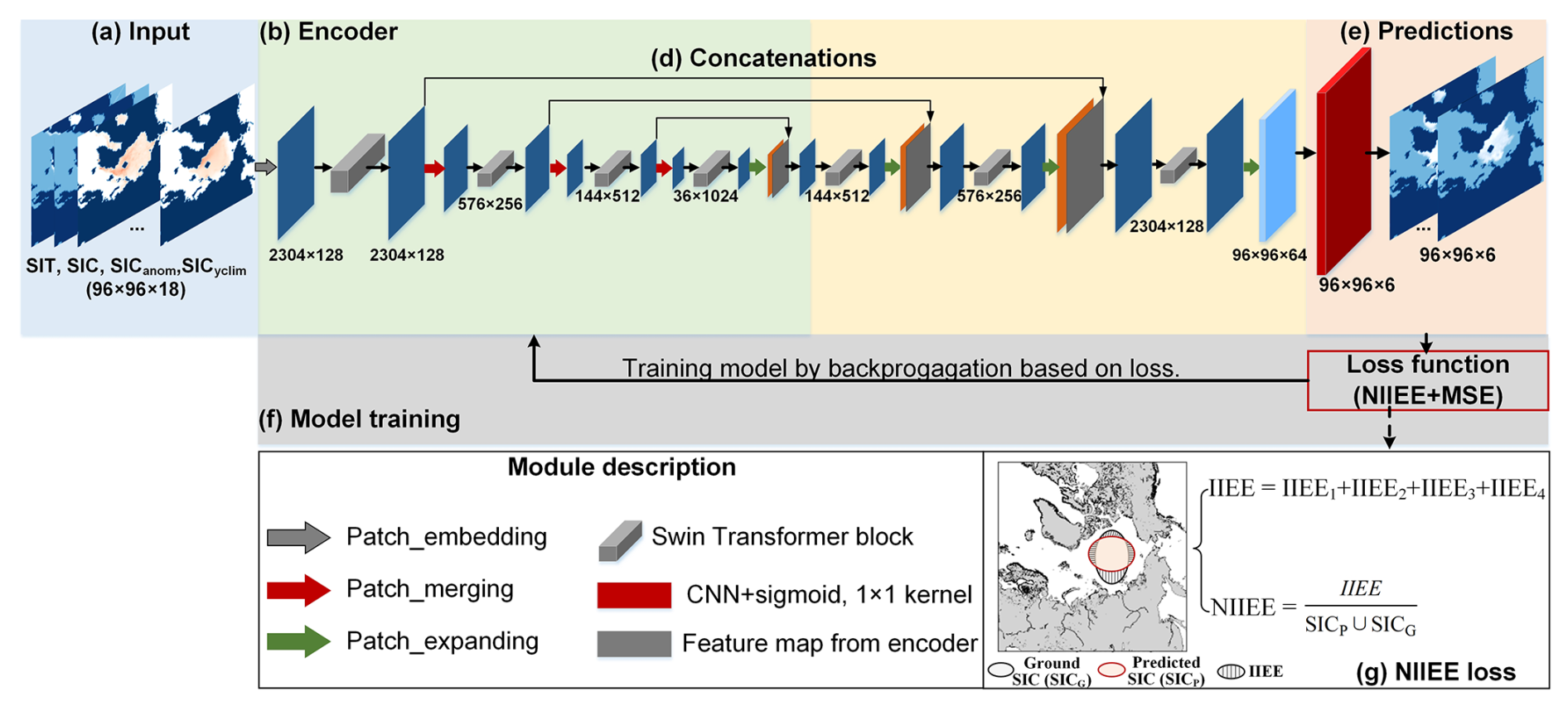
Figure 1 Framework of the model SICNet_season. (a) Input consists of SIT of the last 3 months, SIC of the last 6 months, SIC anomaly of the last 3 months and SIC climatology of 6 target months ($\mathrm{96}\times \mathrm{96}\times \mathrm{18}$). (b) The encoder comprises four Swin Transformer blocks and three patch-merging operators. (c) The decoder contains three Swin Transformer blocks and four patch-expanding operators. (d) Concatenations connect the feature maps from the encoder and the decoder module. (e) A CNN layer with a sigmoid activation transforms the feature map to the predicted SIC of 6-month leads. (f) Model training procedure. The loss function combines the normalized integrated ice edge error (NIIEE) and the mean square error (MSE).

The input for SICNet_season is a $\mathrm{96}\times \mathrm{96}\times \mathrm{18}$ SIC and SIT sequence, composed of SIT of the last 3 months, SIC of the last si6 months, SIC anomaly of the last 3 months and SIC climatology of the 6 target months (Fig. 1a). We determine the length of the input factors by combining domain knowledge and manual-tuning experiments. The primary domain of knowledge we considered is the spring–fall re-emergence mechanism. This occurs between pairs of months where the ice edge is in the same position, such as in May and December (Blanchard-Wrigglesworth et al., 2011; Day et al., 2014). The spring sea ice anomaly is positively correlated with fall sea ice anomalies, and there is also a weaker re-emergence between fall sea ice anomalies and anomalies of the following spring (Bushuk et al., 2015). Therefore, we set the initial input length of the SIC–SIT–SIC anomaly as 6 months. We change the input length manually (from 6 to 1 in step one) to fine-tune the deep learning model to find the best-matched length for each factor. The SIC climatology of the target months provides an essential mean state of the prediction SIC. It represents the monthly cycle signal that IceNet has considered (Andersson et al., 2021).

The input is fed into the encoder to capture spatiotemporal correlations among SIC–SIT data sequences at different levels to form multi-scale correlation maps. The encoder comprises four Swin Transformer (Liu et al., 2021b) blocks and three patch-merging operators (Fig. 1b). A Swin Transformer block is a transformer unit integrated with shifted windows (Liu et al., 2021b). A transformer operator captures global dependencies through an attention mechanism. The shifted windows help the transformer operator capture local dependencies like the convolution operator. Therefore, local and global spatiotemporal dependencies among sea ice sequences can be captured. The patch-merging operator downscales the captured feature maps like the pooling layer in CNN models. The decoder upscales the feature maps through the patch-expanding operator and Swin Transformer blocks (Fig. 1c). The extracted correlation maps of the encoder and decoder are stacked to form fused spatiotemporal maps (Fig. 1d). A CNN layer transforms the decoded feature maps into the same shape as the target SIC sequence. Here, it is a $\mathrm{96}\times \mathrm{96}\times \mathrm{6}$ array (Fig. 1e). As the range of SIC is 0–1, we employ the sigmoid function to activate the last feature map to transform the predicted values to 0–1.

During the training procedure, the loss is calculated between the predicted and ground values. Then, the model's parameters are trained by minimizing the loss value literately. We will explain the loss function in the following section.

3.2 Integrated ice-edge-constrained loss function

For a deep learning model, the loss function is crucial during the training procedure as it guides the optimization of the model's parameters. Here, the loss is the difference between the predicted values and the ground ones from NSIDC. Generally, the mean square error (MSE) is a fundamental loss function for prediction tasks. The MSE measures the mean state for all predicted values and cannot reflect the spatial differences between two-dimensional SIC patterns. To address the issue, we proposed a normalized integrated ice edge error (NIIEE) loss function that considers the spatial distribution of SIC to constrain the model's optimization (Fig. 1g).

The NIIEE loss is based on the integrated ice edge error (IIEE), a professional metric for sea ice predictions. The IIEE represents the error regions the prediction model overestimated and underestimated (Goessling et al., 2016). It measures the spatial similarity between two two-dimensional SIC patterns. Initially, the IIEE binaries the SIC by 15 % to describe the SIE. For the SIC prediction here, we do not perform binarization. Let P_SIC and G_SIC represent the predicted and ground SIC; the IIEE is calculated with Eq. (1). We normalize IIEE to the range of 0–1 to form the NIIEE loss with Eq. (2). If the NIIEE loss is 0 then the predicted SIC and the ground SIC will match spatially and numerically. The fundamental MSE loss has been demonstrated to be adequate for prediction tasks. If the number of all predicted values is N, the MSE is calculated with Eq. (3). We combine the NIIEE with MSE to be the loss function of SICNet_season. A constant scale factor, 0.01, is multiplied by NIIEE to balance its range with that of MSE; see Eq. (4).

$$\begin{array}{}\text{(1)}& {\displaystyle }\mathrm{IIEE}=\left(P_{\mathrm{SIC}}\cup G_{\mathrm{SIC}}\right)-\left(P_{\mathrm{SIC}}\cap G_{\mathrm{SIC}}\right)\text{(2)}& {\displaystyle }\mathrm{NIIEE}={\displaystyle \frac{\mathrm{IIEE}}{P_{\mathrm{SIC}}\cup G_{\mathrm{SIC}}}}=\mathrm{1}-{\displaystyle \frac{P_{\mathrm{SIC}}\cap G_{\mathrm{SIC}}}{P_{\mathrm{SIC}}\cup G_{\mathrm{SIC}}}}\text{(3)}& {\displaystyle }\mathrm{MSE}={\displaystyle \frac{\sum (P_{\mathrm{SIC}}-G_{\mathrm{SIC}}{)}^{\mathrm{2}}}{N}}\text{(4)}& {\displaystyle }\mathrm{Loss}=\mathrm{0.01}\times \mathrm{NIIEE}+\mathrm{MSE}\end{array}$$

4 Experiments

4.1 Model training

The model is trained on a computer station with an NVIDIA Tesla V100 32-GB card. The training and test samples are constructed by step-by-step sliding. The testing period is 2000–2019. The leave-1-year-out strategy is adopted to train and/or evaluate our SICNet_season model. For example, if the testing year is 2000, the training set is from 1979 to 1999 and from 2001 to 2019. The leave-1-year-out strategy is widely adopted by statistical models to maximize the sample volume while obtaining a multi-year evaluation (Wang et al., 2022; Yuan et al., 2016). The validation set is split by 20 % from the training set. We set the batch size to be 8 and the initial learning rate to be 0.0001. We employ the early-stopping strategy to break the training procedure when the validation loss does not decrease. The model is trained three times to eliminate random errors. The testing set is run on three trained models, and the mean values are adopted as the final predictions. Data from the 4 most recent years, 2020–2023, are employed to verify the model's generalizability. Data from these 4 years do not participate in the training stage. They are fed into the trained models obtained by the leave-1-year-out strategy to obtain the predictions. The predictions are the mean values of the 20 trained models.

4.2 Evaluation metrics

The mean absolute error (MAE), binary accuracy (BACC) and detrended ACC are evaluation metrics. The MAE is for SIC, and the other two metrics are for SIE. To accurately calculate the metrics, we use the maximum observed monthly SIE since 1979 to mask the predictions. Assuming that the predicted and truth values of the ith grid are p_i and g_i, the number of validation grids is N. The MAE values are calculated with Eq. (5). The BACC of time t is obtained by using a value of 1 and subtracting from this the ratio of IIEE to the area of the activated grid cell region (the maximum observed SIE during 1979–2019) of t with Eq. (6). The detrended ACC of SIE is the anomaly correlation coefficient of two detrended SIE series. Each SIE series has 20 elements from 2000 to 2019.

$$\begin{array}{}\text{(5)}& {\displaystyle }\mathrm{MAE}={\displaystyle \frac{\sum _{\mathrm{1}}^N\mathrm{|}{p}_i-g_i\mathrm{|}}{N}}\text{(6)}& {\displaystyle }\begin{array}{rl}& \mathrm{BACC}=\\ & \left(\mathrm{1}-{\displaystyle \frac{\mathrm{IIEE}}{\mathrm{area}\mathrm{of}\mathrm{the}\mathrm{activated}\mathrm{grid}\mathrm{cell}\mathrm{region}}}\right)\times \mathrm{100}\mathit{\%}\end{array}\end{array}$$

4.3 Model skill in seasonal predictions

We compare SICNet_season with Persistence and SEAS5 to validate our model's ability to optimize the predictions around the SPB. The persistence is the anomaly persistence model. It assumes that the anomaly is constant in time and estimates the target SIC values by adding the current anomaly to the climate mean state at the target time, widely adopted as a benchmark for sea ice prediction (Wang et al., 2016). The SEAS5 is a new seasonal forecast system from the ECMWF that shows excellent sea ice prediction skills (Johnson et al., 2019). A BACC value of 100 % indicates that the predicted SIE matches the observed SIE by 100 % spatially. The metrics are calculated for 20 testing years, 2000–2019, in a leave-1-year-out training–testing strategy. As the SPB occurred in the target summer month, we focus on the 4 summer months of June to September.

Figure 2 shows the detrended ACC and BACC of the target months, June–September, based on 6-month-lead predictions. As shown in Fig. 2a and b, the predictions of Persistence and SEAS5 show an apparent SPB: the detrended ACC drops sharply when the predictions are made earlier than May, with a maximum ACC gap between 2 adjacent lead months marked by black lines. Taking September, for example, the detrend ACC is 56.39 % for Persistence when the prediction is made in June (3-month lead). Then, it decreases to 26.59 % in May's prediction (4-month lead); see Fig. 2a. For SEAS5, the ACC of June's prediction is 83.94 %, which then drops to 59.91 % for May's prediction, forming a 24.03 % ACC gap; see Fig. 2b. Although the SICNet_season prediction also shows an SPB feature (see the black line in Fig. 2c), the ACC of May's prediction is improved to 67.61 %, and the ACC gap is reduced to 15.6 %. Furthermore, the ACC difference is calculated between SICNet_season and Persistence and SEAS5. Compared with Persistence, SICNet_season improves the ACC in most predictions; see Fig. 2d. The ACC improvements along the SPB flag are more than 30 % on average (the lead months right on the black line in Fig. 2d). Compared with SEAS5, SICNet_season also improves the prediction skill of the SPB. When the target months are June and July, SICNet_season shows a much higher prediction skill than SEAS5 in 4- to 6-month-lead predictions; see Fig. 2e. For the target month of September, SICNet_season improves the ACC by 7.70 % or 10.61 % compared to SEAS5 when the prediction is made in May or April (4- or 5-month-lead in Fig 2e). For the target month of August or September, SICNet_season shows lower ACCs than SEAS5 when prediction is made during or before March (5- or 6-month-lead for August or September). However, for the predictions made adjacent to the SPB flag line, SICNet_season achieves larger ACCs than SEAS5 (values right along the black line in Fig. 2e). Therefore, SICNet_season optimizes the SPBs significantly compared to the well-known numerical model.

The BACC of SEAS5 also shows a similar SPB characteristic to the ACC. A sharp BACC drop occurred when the prediction was made during and before May; see the black line in Fig. 2g. The maximum BACC gaps of Persistence and SICNet_season occurred in the second lead month. However, the maximum BACC gap of SICNet_season is about 2 %, much lower than the 10 % gap of Persistence and SEAS5. Compared with Persistence and SEAS5, SICNet_season improves the BACC by more than 10 % in predicting the SIE of August and September (3 to 6-month-lead; see Fig. 2i and j).

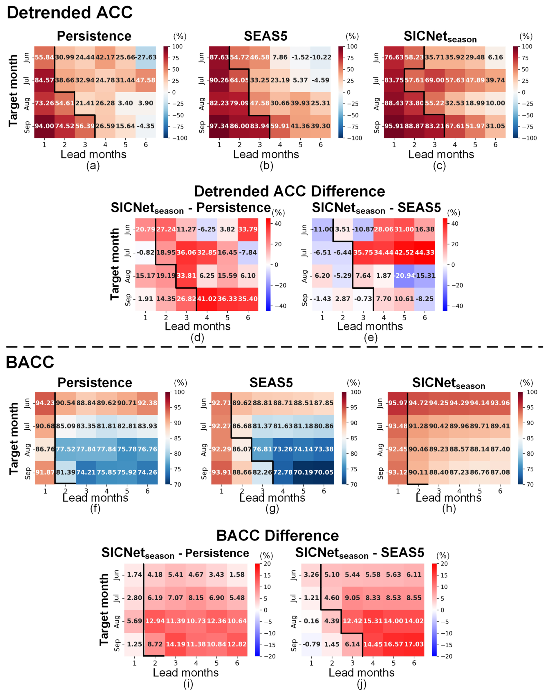
Figure 2 Detrended ACC of SIE and detrended BACC of SIE, as well as the differences between Persistence, SEAS5 and SICNet_season from June to September, averaged for 2000–2019. (a)–(c) Detrended ACC of three models. Two detrend SIE series (predicted and observed) calculate each value. (d)–(e) Detrended ACC differences between SICNet_season and Persistence and SEAS5. (f)–(h) BACC of three models. Each BACC is a mean value of 20 testing years. (i)–(j) BACC differences between SICNet_season and Persistence and SEAS5. The black line indicates the SPB: a maximum decrease between 2 adjacent lead months. The red signifies a high or improvement in ACC and/or BACC, and the blue signifies a decrease.

4.4 Performance in predicting SIC of September

As September's sea ice draws wider attention than other months, we calculate the MAE of the SIC of September predicted by three models. Figure 3 shows the spatial MAE of Persistence, SEAS5 and SICNet_season based on 6 lead months. The MAE in the three models is not very different for the first 2 lead months. When the lead month duration is 1, the MAE of SEAS5 is slightly better than that of Persistence and SICNet_season, indicating that the SEAS5 model performs well in monthly predictions. This result may be due to the good atmospheric initialization in SEAS5, which beat many machine learning and dynamical models in sub-seasonal-scale SIC prediction (Bushuk et al., 2024). However, when the lead month duration is longer than 3, the SEAS5 MAEs are much more than 45 % in the Pacific sector, mainly containing the Beaufort Sea, the Chukchi Sea, the East Siberian Sea and the Laptev Sea; see Fig. 3j–l. SICNet_season reduces the MAEs to 20 %–30 % for most regions in the Pacific Arctic; see Fig. 3q–r. Compared with Persistence, SICNet_season also reduces MAEs by 5 %–10 % in the four mentioned local seas; see Fig. 3d–f. Therefore, SICNet_season significantly reduces the SIC errors of September in seasonal-scale predictions (3- to 6-month lead).

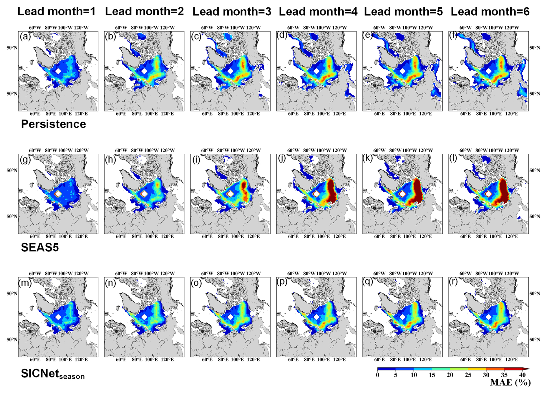
Figure 3 The MAEs of September's predictions are based on three compared models: each value is averaged by 20 testing years. (a)–(g) MAEs of Persistence. (h)–(m) MAEs of SEAS5. (n)–(s) MAEs of SICNet_season.

4.5 SIT contributions to seasonal predictions

We further conduct a comparison experiment to validate the role of SIT data in seasonal predictions based on SICNet_season. The model without SIT as an input is named SICNet_{season_nosit}. The other settings for SICNet_{season_nosit} are the same as those for SICNet_season. The detrended ACC and BACC are shown in Fig. 4.

Without the SIT data as input, the model's prediction skill drops noticeably in 3- to 6-month-lead predictions; see Fig. 4a. For the target month of September, the detrend ACC is 76.41 % when the prediction is made in June (3-month lead). Then, the ACC drops to 26.43 % for May's prediction (4-month lead). By including SIT data as input, the ACC of May's prediction is improved by 41.18 % in the model SICNet_season; Fig. 4c. For the target month of August, the ACC improvement for May's prediction (3-month lead) as a result of including SIT data is 42.44 %. Therefore, the SIT data are important to improve the model's prediction skill with regard to SPB.

For the target months of August and September, the BACCs of SICNet_{season_nosit} show an apparent drop in 3- to 6-month-lead predictions. By including SIT data as the model's input, the BACC improvement is 0.95 % and 2.02 % for the target months of August and September for May's predictions; see Fig. 4f. Then, we calculate the MAE of the target month of September; see Fig. 5. The MAEs of the first 2 lead months are similar for the two models. When the lead month duration is larger than 3, the MAEs of SICNet_{season_nosit} in the Beaufort Sea, the East Siberian Sea and the Laptev Sea are 30 %–45 %, as shown by the red circles in Fig. 5d–f. By including SIT data, the MAEs in the three mentioned regions are reduced to 20 %–35 % by SICNet_season, as shown with the red circles in Fig. 5j–l. Therefore, including SIT data reduces the errors of September's SIC by more than 10 % in seasonal-scale predictions.

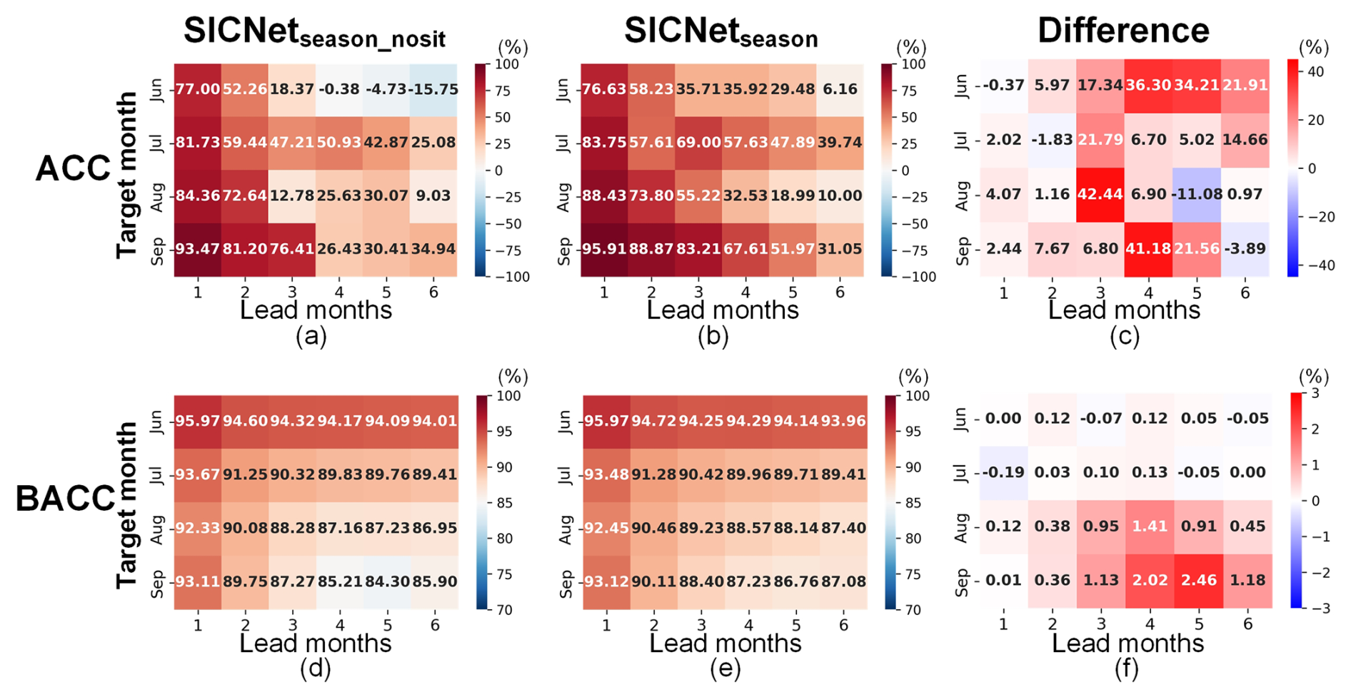
Figure 4 Detrended ACC of SICNet_{season_nosit} (a) and SICNet_season (b). (c) ACC difference obtained with SICNet_season minus SICNet_{season_nosit}. BACC of SICNet_{season_nosit} (d) and SICNet_season (e). (f) BACC difference as in (c). The red signifies a high or improvement in ACC and/or BACC, and the blue signifies a decrease.

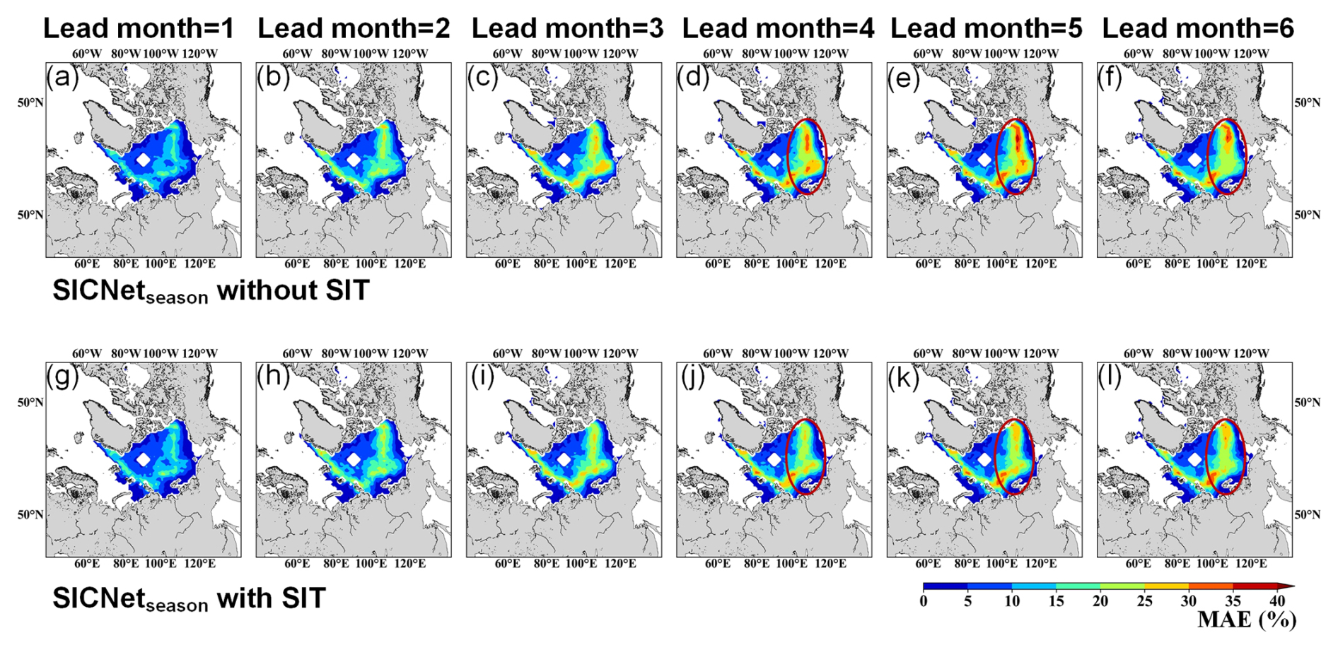
Figure 5 The MAEs of September's SIC predicted by SICNet_season and SICNet_{season_nosit}. Each value is averaged by 20 testing years. (a)–(g) MAE of SICNet_{season_nosit}. (h)–(m) MAE of SICNet_season. The red cycles mark the regions where the MAE is typically reduced as a result of including SIT data.

4.6 Generalizability in predicting the SIEs of 2020–2023

To verify our model's generalizability in predicting the SIEs of recent years, we employed the 20 trained models to predict the SIE of the 4 most recent years of 2020–2023. The 20 models are trained for 2000–2019, as mentioned in the earlier sections. The data from the period 2020–2023 are “blind” for the models. The mean values of the 20 models' predictions are the final predictions. As the temporal span of 4 years is too short for calculating ACC, we use the BACC as the metric (Fig. 6). Compared with Persistence and SEAS5, SICNet_season achieves higher BACCs in predicting the SIEs of August and September. For the target month of September, the BACC of SICNet_seaon is 10 % higher than those of the other two models in 3- to 6-month-lead predictions.

We draw the observed and predicted September SIEs of 2020, 2022 and 2023 in Fig. 7. The September SIEs in 2020 and 2023 (4.0×10⁶ and 4.37×10⁶ km²) are the second and sixth lowest recorded in the Arctic since 1979. The SIE in September 2022 (4.90 mil km²) has been so large since 2015. We focus on the seasonal-scale predictions with 4- to 6-month leads. Our SICNet_season model shows obvious advantages over SEAS5 and Persistence. For predictions made during or before May, with lead months of 4 to 6, the BACCs of SICNet_season are much higher than those of Persistence and SEAS5; see Fig. 7. For May's prediction, our model achieved a BACC of 82.25 %, 90.39 % and 82.08 % in 2020, 2022 and 2023, more than 10 % higher compared to Persistence and SEAS5; see Fig. 7a, d and g. Therefore, the SICNet_season model achieves good generalizability in predicting the SIEs of 2020–2023.

Figure 6 BACC of 2020–2023. (a) Persistence, (b) SEAS5 and (c) SICNet_season. Each value is a mean value of the 4 testing years. The horizontal axis represents the 6 lead months, and the vertical axis represents the target months of June to September. The red signifies a high or improvement in ACC and/or BACC, and the blue signifies a decrease.

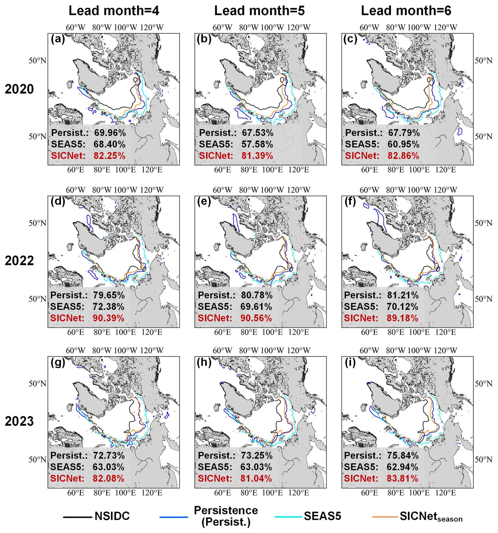
Figure 7 Predicted September SIEs and their BACCs of 2020, 2022 and 2023 for 4- to 6-month leads by Persistence, SEAS5 and SICNet_season. (a)–(c) 2020, (d)–(f) 2022 and (g)–(i) 2023.

4.7 Comparison with the representative deep learning model

We compare SICNet_season against the representative deep learning sea ice prediction model, the U-Net (IceNet-inspired) model. IceNet is a seasonal sea ice prediction model that performs state-of-the-art SIE probability prediction (Andersson et al., 2021). It is a CNN-based U-Net model for classification tasks, and it outputs the probability of three classes: open water (SIC ≤ 15 %), marginal ice (15 % < SIC < 80 %) and full ice (SIC ≥ 80 %). Differently, our SICNet_season outputs the 0 %–100 % range SIC values. The IceNet inputs consist of 50 monthly mean variables, including SIC, 11 climate variables, statistical SIC forecasts and metadata. The original IceNet model has some unique designs in terms of inputs and training strategy. As we focus on the differences in model structures, we construct a U-Net (IceNet-inspired) model for comparison.

We set the inputs (including SIT data) of U-Net (IceNet-inspired) to the same ones as SICNet_season. The loss function is also set as the NIIEE together with the MSE. We set the output layer of U-Net (IceNet-inspired) as a sigmoid activation function to output continuous values of 0 %–100 %. We also change the number of CNN filters to make the number of training parameters in U-Net (IceNet-inspired) equal to that in SICNet_season, about 140 million. The training and testing settings of U-Net (IceNet-inspired) are the same as those of SICNet_season. U-Net (IceNet-inspired) is trained using the same leave-1-year-out strategy as SICNet_season. For example, if the testing year is 2019, the training set is made up of data from the period 1979–2018, and the testing data are from 2019. Then, the testing data are moved to 2018; the remaining data (1979–2017, 2019) make up the training set. For each training–testing pair, the model is trained three times to eliminate randomness, and the final prediction for the testing data is the mean value of the three models.

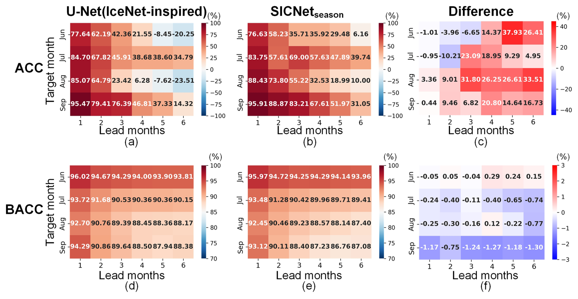
Figure 8 Detrended ACC of U-Net (IceNet-inspired) (a) and SICNet_season (b). (c) ACC difference obtained by SICNet_season minus U-Net (IceNet-inspired). BACC of U-Net (IceNet-inspired) (d) and SICNet_season (e). (f) BACC difference as in (c). The red signifies a high or improvement in ACC and/or BACC, and the blue signifies a decrease.

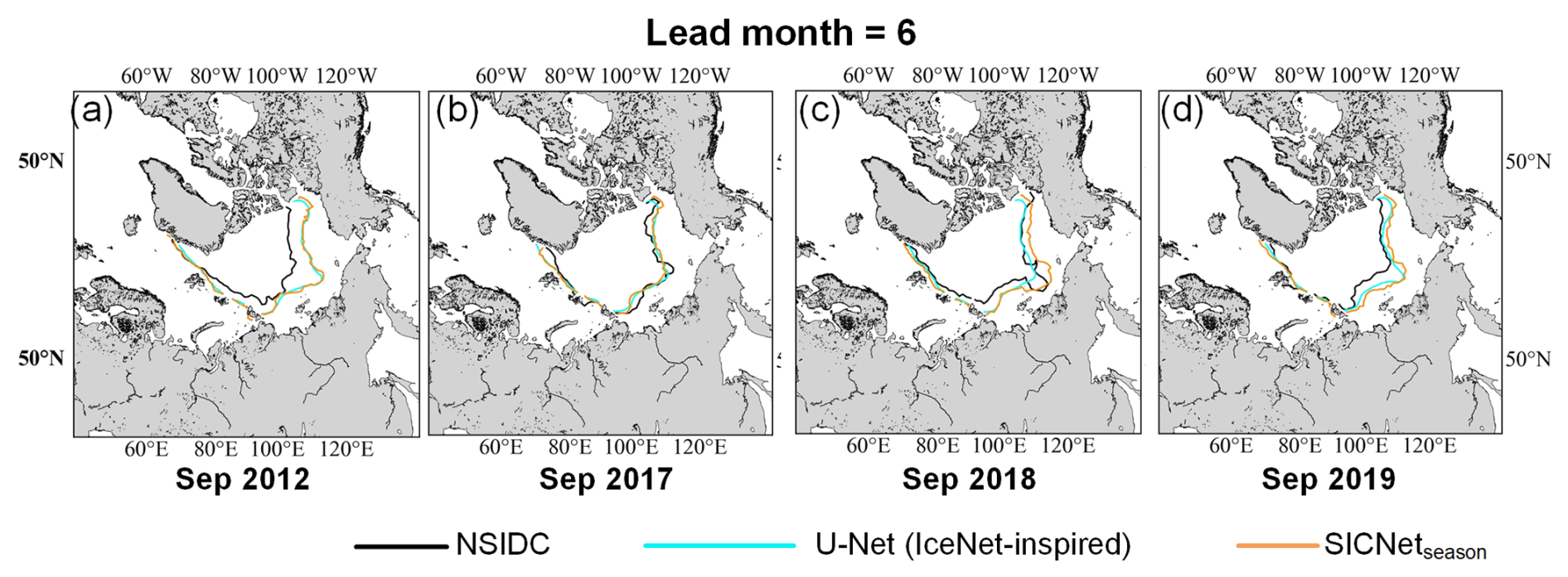
Figure 9 The predicted September SIEs of U-Net (IceNet-inspired) and SICNet_season in for 6-month lead: (a) 2012, (b) 2017, (c) 2018 and (d) 2019.

Figure 8 shows the detrend ACC and BACC, as well as the differences between the two models. Compared with the U-Net (IceNet-inspired) model, our SICNet_season model significantly improves the ACC for most predictions; see Fig. 8c. For the target months of August and September, the SPB feature is obvious in U-Net (IceNet-inspired): the maximum ACC gap is about 40 % and 30 %, respectively, for predictions made in May and June; see Fig. 8a. Our SICNet_season model optimizes the ACC gap with an improvement of 31.8 % and 20.8 % for May's predictions; Fig. 8c. The ACC improvements are also larger than 15 % for predictions made before May. Therefore, compared with the state-of-the-art deep learning model U-Net (IceNet-inspired), our model achieves more skillful seasonal predictions by optimizing the predictions around the SPB.

Unlike the ACC values, the BACC values of U-Net (IceNet-inspired) are more significant than those of SICNet_season for most predictions; see Fig. 8f. This result implies that U-Net (IceNet-inspired) depends more on SIE trends than SICNet_season. This difference can be attributed to the distinct fundamental units employed by the two models. The U-Net (IceNet-inspired) model is a CNN-based model, and the weight-sharing mechanism of convolutional kernels forces the model to capture the most “common” local dependencies spatially. Though representative, these common local dependencies tend to yield smoother model outputs. SICNet_season is a transformer-based model. The attention mechanism of the transformer can capture global dependencies without weight-sharing. As a result, “personalized” global dependencies are extracted, and the output is not smooth like the output of a CNN-based model. The common local dependencies have more apparent trend features than the personalized global dependencies. Figure 9 shows the September SIEs predicted by U-Net (IceNet-inspired) and SICNet_season in the 6-month lead. The SIEs of U-Net (IceNet-inspired) are smoother than those of SICNet_season. For 2012 and 2017, the SIE locations of the two models are very similar. For the other 2 years, the SIEs of U-Net (IceNet-inspired) match the observed SIEs better than those of SICNet_season. However, the SIEs of U-Net (IceNet-inspired) are over-smoothed and fail to characterize some abnormal characteristics, such as the SIE in September 2018; see Fig. 9c.

Therefore, our transformer-based SICNet_season is more skillful than the representative CNN-based model U-Net (IceNet-inspired) in optimizing the predictions around the SPB. SICNet_season exhibits a lower dependency on SIE trends and fewer smooth results than the CNN-based model.

5 Conclusions

This study develops a deep learning model, SICNet_season, to predict the Arctic SIC on a seasonal scale. The model is derived from a Swin-UNet architecture. It inputs the historical SIC, SIT and SIC climatology of target months and predicts the SIC of the next 6 months. A spatially constrained loss function NIIEE is employed to train the model by considering the sea ice distribution. We employ a 20-year (2000–2019) testing set to validate the model's performance. The summer season, June to September, is the target period. The detrend ACC, BACC and MAE are metrics. Comparison experiments with Persistence and seasonal predictions of SEAS5 are made to validate our model's performance. In particular, an ablation experiment is carried out to investigate the role of SIT data in optimizing the predictions around the SPB. A generalizability experiment with data from the last 4 years, 2020–2023, is carried out – the seasonal predictions of September SIEs are analyzed. Finally, we discuss the advantages and disadvantages of our model and the typical CNN-based model, U-Net (IceNet-inspired). Given the mentioned efforts, our study draws the following conclusions.

First, our deep learning model, SICNet_season, is skillful in predicting the Arctic sea ice seasonally. Compared with the dynamic model SEAS5, SICNet_season optimizes the SPB significantly. The detrended ACC of September SIE predicted by SICNet_season in May and April is improved by 7.7 % and 10.61 % over the ACC predicted by SEAS5. Compared with the anomaly persistence benchmark, the mentioned improvement is 41.02 % and 36.33 %, respectively. Our deep learning model significantly reduces the prediction errors of September's SIC on seasonal scales compared to SEAS5 and Persistence, a 20 %–30 % reduction measured by MAE.

Second, the spring SIT data are key in optimizing the predictions around the SPB, contributing to a more than 20 % ACC enhancement in September's SIE at 4 to 5-month-lead predictions. By including SIT data, the MAEs in the Beaufort Sea, the East Siberian Sea and the Laptev Sea are reduced by more than 10 % compared with those without SIT data.

Third, our model achieves good generalizability in predicting the September SIEs of 2020–2023. When predicting the September's SIE in 2020 and 2023 (second and sixth lowest record) in May, SICNet_season achieved a BACC of 82.25 % and 82.08 %, about 12 % and 10 % higher than Persistence and SEAS5.

Fourth, our transformer-based SICNet_season is more skillful than the CNN-based U-Net (IceNet-inspired) model in seasonal sea ice predictions. Our SICNet_season model optimizes the ACC gap with an improvement of 31.8 % and 20.8 % for May's predictions compared to U-Net (IceNet-inspired). SICNet_season exhibits a lower dependency on SIE trends and fewer smooth results than the CNN-based model. This is due to the attention mechanism of the transformer operator extracting personalized global dependencies, while the CNN operator captures the most common local dependencies globally. The common local dependencies smooth the map and depend more on the trend than personalized ones.