NN-TOC v1: global prediction of total organic carbon in marine sediments using deep neural networks

Spatial predictions of total organic carbon (TOC) concentrations and stocks are crucial for understanding marine sediments’ role as a significant carbon sink in the global carbon cycle. In this study, we present a geospatial prediction of global TOC concentrations and stocks on a 5 × 5 arcmin grid, using a novel neural network approach. We also provide and apply a new compilation of over 21 000 global TOC measurements and a new set of predictors, including features such as seafloor lithologies, benthic oxygen fluxes, and chlorophyll-a satellite data. Moreover, we compare different machine learning models based on their performance metrics and predictions and assess their strengths and limitations. For the dataset used, we find that the performance metrics of the models are comparable and that the neural network approach outperforms, on unseen data, methods such as k-nearest neighbours and random forests, which tend to overfit the training data. We provide estimates of mean TOC concentrations and stocks, both on continental shelves and in deep-sea settings across various marine regions and oceans. Our model suggests that the upper 10 cm of oceanic sediments harbour approximately 156 Pg of TOC stocks and have a mean TOC concentration of 0.61 %. Furthermore, we introduce a standardized methodology for quantifying predictive uncertainty using Monte Carlo dropout. The method was applied to our neural network model and underlying features to generate a map of information gain that measures the expected increase in model knowledge, achieved through additional sampling at specific locations, which is pivotal for sampling strategy planning.

1 Introduction

Burial of particulate organic carbon in marine sediments removes carbon dioxide (CO₂) from the atmosphere and generates molecular oxygen (O₂) that accumulates in the atmosphere (Berner, 1982; Hedges and Keil, 1995). It is a key process in the global carbon cycle that largely controls the atmospheric partial pressures of O₂ and CO₂ on geological timescales (Berner, 1982, 2004). The mechanisms controlling concentrations, standing stocks, and degradation and accumulation rates of organic carbon at the seabed are, however, complex and remain a topic of active research (Arndt et al., 2013; Burdige, 2007; Hedges and Keil, 1995; LaRowe et al., 2020b; Bradley and Arndt, 2022). Furthermore, present estimates of the spatial distribution of sedimentary carbon concentrations and stocks across the global ocean, including shelf regions, are limited due to sparse data and the high spatial variability observed in shelf deposits (Atwood et al., 2020; Diesing et al., 2021; Lee et al., 2019; Legge et al., 2020; Seiter et al., 2004). An improved map of global organic carbon concentrations and stocks in marine surface sediments, including the continental shelf, could, hence, help to better understand processes governing the turnover and accumulation of organic carbon at the seabed.

Sedimentary organic carbon concentrations are typically reported as total organic carbon (TOC in weight percent), which includes particulate organic carbon bound to sediment grains and a minor contribution by organic carbon dissolved in sediment porewater (Hedges and Keil, 1995). TOC varies between different geological environments (Emerson and Hedges, 1988). Fine-grained shelf and delta sediments deposited close to river mouths typically contain 0.5 %–1.0 % TOC at 0–10 cm sediment depth (Berner, 1982). A major fraction of TOC deposited in these environments (up to 67 %) is not formed by marine plankton but is produced by land plants (Burdige, 2005). Shelf regions where neritic carbonates are formed by corals and other organisms at the seabed contain about 1 % TOC (Berner, 1982). However, large parts of the continent shelf (about 50 %–70 %) do not receive sediment inputs and are covered by relict sands (Emery, 1968; Hall, 2002) that contain only minor amounts of TOC (about 0.1 %). Typical deep-sea sediments, which are not associated with high-productivity regions, contain about 0.2 %–0.4 % TOC (Baturin, 2007; Berner, 1982; Lee et al., 2019; Seiter et al., 2004). In oceanic upwelling regions with high productivity, large amounts of TOC are rapidly deposited at the seabed such that sedimentary TOC concentrations are usually higher than 1 % and may reach up to 10 % (Berner, 1982; Lee et al., 2019; Seiter et al., 2004). Elevated TOC values are also reported for surface sediments deposited in the Arctic Ocean (1.0 %) and the deep basins of the Black Sea (2.0 %) (Berner, 1982; Lee et al., 2019; Seiter et al., 2004). Considering these observations, the global mean TOC concentration in both shelf and deep-sea sediments seems to be close to 0.5 % to 1.0 %.

The inventory or standing stock of TOC in surface sediments (in mass of carbon per seafloor area) is calculated by multiplying TOC concentrations by the dry bulk density of sediments and the thickness of the considered surface layer. Different methods have been applied to derive the standing stock of TOC at regional and global scales. An early estimate based on limited data and expert knowledge concluded that the global TOC stock is 146 Pg TOC for a 30 cm surface layer (Emerson and Hedges, 1988). The first estimate of the global TOC inventory derived by a machine learning approach (k-nearest neighbours – kNNs) using an extended database (5623 data points) yielded a global inventory of 87 ± 43 Pg TOC in the top 5 cm layer (Lee et al., 2019). In subsequent publications with an extended database (11 574 sediment cores) and a more advanced machine learning approach (random forest model), the global inventory was estimated as 2322 Pg TOC for the top 1 m of the sediment column (Atwood et al., 2020). This inventory exceeds the global TOC inventory in terrestrial soils and suggests that TOC in marine surface sediments is the largest TOC pool at Earth's surface (Atwood et al., 2020). Another estimate of the global TOC inventory was derived by reactive transport modelling of sedimentary processes employing a range of global datasets (LaRowe et al., 2020a). This model yields a global inventory of 170 Pg TOC for the top 10 cm affected by biological mixing processes.

Since about 70 % of Earth's surface is covered by oceans and sampling sediments at the seafloor is costly, data coverage will always be sparse. Therefore, advanced methods are required to derive spatial information on sediment properties from a limited number of point measurements. Machine learning approaches, which have rapidly advanced in recent years, are the most promising approach to tackling this challenge. So far, k-nearest neighbours and random forest models have been applied to derive global maps of sediment porosity (Martin et al., 2015), TOC concentration (Lee et al., 2019), TOC inventory (Atwood et al., 2020), sedimentation rate (Restreppo et al., 2021, 2020), and regional estimates of TOC accumulation rates (Diesing et al., 2021). However, machine learning techniques have their own challenges and limitations. Overfitting issues are often encountered, and a standardized approach for estimating predictive uncertainty has not yet been established (Lee et al., 2019).

Given these challenges, this paper aims to derive more robust maps of TOC concentrations and inventories for the global ocean. These maps, including the continental shelf, are based on a new, larger TOC measurement database and an extended collection of predictors to improve the accuracy of predictions for highly heterogeneous and undersampled geological settings. We compiled an enlarged database of TOC concentrations in surface sediments with 21 125 entries and applied a deep neural network (DNN) as a more advanced machine learning approach that considers the non-linear relationships between TOC and other geological features. The global ocean was divided into two different domains (shelf and deep sea), and the network was trained separately for each of these domains. Moreover, we introduced a standardized methodology called Monte Carlo dropout to quantify predictive uncertainties in the DNN model and derive information gain to guide future sampling efforts.

2 Materials

2.1 Features

An extensive repository of features from both the sea surface and the seafloor at a 5 × 5 arcmin grid resolution has been compiled using previously reported feature lists (Lee et al., 2019; Restreppo et al., 2021; Hart-Davis et al., 2021) that include a range of oceanographic, geological, geographic, biological, and biogeochemical parameters. It is worth noting that oceanographic features are updated very often from newer models and measurements, and some of the features used here might be outdated. Features deemed irrelevant to TOC distributions (e.g. crustal and mantle properties, distance to the plate boundary, continental ridges, and trenches) were excluded. Additional features that may influence TOC distributions were added to improve TOC predictions. These include total oxygen uptake (respiration rates) at the seabed (Jørgensen et al., 2022), sediment lithology (Garlan et al., 2018), tidal velocities (Hart-Davis et al., 2021), and chlorophyll-a concentrations at the sea surface (NASA, 2014).

Ninety-nine raw feature grids are compiled for a comprehensive representation of the marine environment, providing the necessary input for the neural network analysis in this study to predict TOC concentrations in marine sediments. Most of these features are easily measurable from the sea surface by e.g. satellite observations, making them a reliable dataset compared to the less accessible properties of the seafloor. Some of the seafloor feature grids used in this work were previously generated from raw data using machine learning methods (e.g. a porosity grid provided by Martin et al., 2015). Others were reprocessed in this work to achieve global coverage at a resolution of 5 × 5 arcmin (e.g. sediment lithology, Garlan et al., 2018).

Neighbourhood information was incorporated for a subset of the features. Specifically, 40 of the 99 initial features were averaged spatially using a 50 km radius (Lee et al., 2019). Spatial averaging was applied when TOC concentrations are assumed to be affected not only by the local feature value, but also feature values in the surrounding area. This approach was used for selected physical (e.g. current velocity), chemical (e.g. dissolved compounds), and biological (e.g. bio-fauna abundance) parameters.

Overall, a total of 139 features, including 99 original features and 40 additional spatially averaged features, is used in the model. The complete feature list is presented in Appendix A.

2.2 TOC data

The dataset for TOC concentrations (in weight percent) utilized in this study has been compiled from multiple sources. It includes global datasets (Seiter et al., 2004; Romankevich et al., 2009; van der Voort et al., 2021; Paradis et al., 2023) and regional datasets for the northern Gulf of Mexico (Beazley, 2003) and the North Sea (Wenyen Zhang, personal communication, 2023, HEREON). Each label represents a known measurement (TOC concentration) and is paired with the nearest grid point on the 139-feature grids via L2 distance computation, resulting in the association of a feature vector with each label. For those stations where TOC is reported as function of sediment depth, we calculated the mean TOC concentration for the top 10 cm and used this mean as the model label. For many stations, values are only reported for the top 1–2 cm (around 19 000 measurements). We included these stations in our model since they contain valuable information, but we acknowledge that they may be somewhat higher than those integrated over the top 10 cm since TOC concentrations tend to decrease with sediment depth due to ongoing TOC degradation. However, most sediments deposited on the continental shelf and in high-productivity regions of the open ocean are affected by intense biogenic and physical mixing processes (Boudreau, 1997) such that the downcore TOC decrease is usually small within the mixed surface layer (0–10 cm sediment depth). The labelled data are pre-processed to enhance the reliability and robustness of the dataset for subsequent model development and validation. We first searched for duplicates in our combined database that may arise when the same data are reported in multiple databases. They were removed from the combined database when longitudes, latitudes, and TOC concentrations were identical. Moreover, coastal regions often exhibit clustered measurements, potentially resulting in shared feature vectors, as all the measurements lie in the same feature grid cell. To mitigate this, a variance assessment is conducted. Labels that share the same feature vectors, exhibiting high variance (the standard deviation of these labels is higher than 20 % of the maximum of these labels) are excluded, while those with low variance are averaged, and the shared feature vector is assigned. Also, some data points situated in close proximity to land were not captured adequately by the 5 × 5 arcmin grid. To address this, reasonable values are assigned by interpolating from the nearest points, ensuring the overall quality of the dataset. Our database includes a total of 110 149 data points that have been consolidated as discussed above such that the final TOC database employed in the model is composed of 21 125 entries (Fig. 1). Both the datasets for the labels and features can be downloaded at https://doi.org/10.5281/zenodo.11186224 (Parameswaran et al., 2024b).

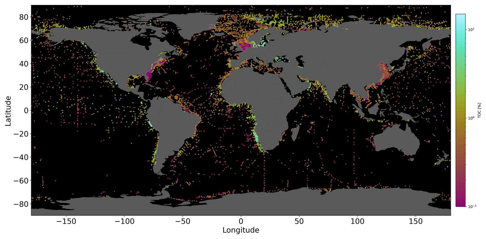
Figure 1 Quantitative TOC measurements (i.e. labels) acquired from various sources (Seiter et al., 2004; Romankevich et al., 2009; van der Voort et al., 2021; Beazley, 2003; Paradis et al., 2023). Notably, data point clusters are observed in close proximity to coastal regions. The colour maps used for the figures in this paper are from Crameri (2023) and Thyng et al. (2016).

3 Methods

The primary objective of this study is to build a supervised prediction model that uses feature grid maps as inputs to predict TOC concentrations as outputs. Additionally, we aim to quantify prediction uncertainties using Monte Carlo dropout and information theory techniques. The supervised model is trained using the set of labels (TOC data) and their corresponding feature vectors. Due to the non-linearity in the relationships between data and features, we choose deep-learning models, which are good at understanding such patterns. Deep neural networks (DNNs) transform data non-linearly with non-linear activation functions such as ReLU (rectified linear unit), a piecewise linear function that outputs 0 for negative inputs and the input itself for positive inputs, introducing non-linearity into the DNN. Therefore, even after one layer, multi-collinearity in the data is eliminated. In our case of a deep neural network, the final output is controlled by numerous combinations of ReLU functions involving higher-order interactions of original features (De Veaux and Ungar, 1994).

3.1 Deep-learning model

Deep neural networks have achieved state-of-the-art results in a variety of tasks in ocean observation, prediction, and forecasting of ocean phenomena (Song et al., 2023). DNN architectures, which are intrinsically non-parametric and non-linear, are less susceptible to the curse of dimensionality. They capture complex relationships between data and features at different levels of abstraction through their hierarchical nature, which makes them well-suited to resolving highly complex geoscientific problems (LeCun et al., 2015).

Here, we use a multi-layer perceptron (MLP), feed-forward DNN to predict global TOC in sediments and introduce a new approach to mapping uncertainty in predictions that serves as a quantifiable measure of information gain from sampling. To further improve our predictions, the global ocean was separated into a continental shelf and deep-sea region using the 200 m water depth horizon as a boundary. Two separate models were trained for these regions (shelf: 0–200 m, deep sea: > 200 m) to consider the different processes that drive sedimentation and control TOC values in the deep-sea and shelf environments. The same set of features is used for both regions, but the interplay of these features differs between the contrasting environments. The weights and biases in the DNN are initialized using the technique proposed by He et al. (2015). Batch normalization (which normalizes the inputs of each layer for faster and more stable training) and dropout (which assigns a probability of being deactivated to each node during training and thus prevents overfitting) are applied to each layer for regularization. ReLU is used as the activation function.

The Monte Carlo dropout method is implemented here to estimate uncertainty in the DNN model, leveraging dropout layers as approximate Bayesian inferences (Gal and Ghahramani, 2016). It gives us an ensemble of predictions from different subsets of neurons in the same DNN model. Kullback–Leibler (KL) divergence is used to map information gain from the quantified predictive uncertainty. In the field of information theory, KL divergence represents the information gain and is defined as the difference of the cross-entropy between the observation and prediction of an event and the entropy in the observation of the event (Kullback and Leibler, 1951). In our context, the predicted distribution arises from the Monte Carlo dropout prediction ensemble, while the reconstructed observed distribution is modelled with a normal distribution, with the predicted value as a mean and a standard deviation of 0.05 TOC % arising from both technical handling and the precision of the weighting tool (Pape et al., 2020).

Uncertainty and information gain are inherently associated insofar as there cannot be high information gain without high uncertainty. However, information gain also depends on the observation probability distribution and is constrained by it. In other words, information gain measures the expected increase in model knowledge achieved through field sampling at a specific location. This concept provides a strategic guide for determining optimal sampling strategies: taking samples in regions with the highest information gain values is the most efficient way of refining our model’s representation of the real world. The mathematical formulation of entropy, cross-entropy, and information gain is detailed in Appendix B.

4 Results and discussions

Understanding the global distribution of TOC concentrations and stocks is crucial for advancing our knowledge of the carbon cycle and sedimentary environments worldwide. Before delving into the prediction maps from the DNN, we first compare the performance of three methods: DNNs, kNNs, and random forests. Separate models are run for the deep-sea and continental shelf regions, and the outcomes are summarized in Table 1. For kNN, five neighbours were utilized for the continental shelves and four for the deep sea, based on a sensitivity analysis with respect to model performance. Random forests employed 100 estimators for both marine regions. The DNN consists of 10 layers with 128 nodes each. The choice of hyperparameters in the models is discussed in Appendix C. This comparison sets the groundwork for a detailed exploration of DNN results. All of the methods were run with the same training–testing splits of the dataset, and the random split is seeded to make the methods reproducible.

Table 1 Comparison of machine learning methods based on performance metrics: Pearson correlation coefficient (Pearson CC), coefficient of determination (R²), and mean squared error (MSE) for predicted values vs. observed labels for the training and testing data. The train:test data ratio is 85:15. The better-performing method, based on the metric, is highlighted in bold.

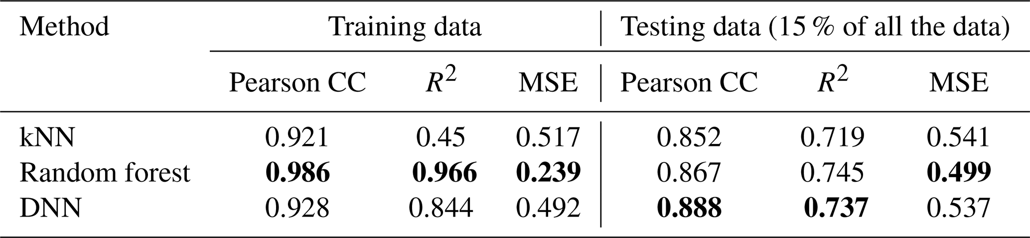
The results of this model comparison show that random forest and kNN algorithms exhibit higher correlation coefficients and superior overall performance in the training dataset than the DNN. However, the DNN outperforms the other two algorithms in the testing data performance (Table 1) for the dataset used. This discrepancy suggests a potential overfitting issue, where the kNN and random forest models may have become specialized in learning the training data. The emphasis on generalization capabilities is crucial in our context due to data scarcity in many regions, making predictions in unexplored areas a priority. The correlation plot between the measured and predicted data shows similar errors for the training and testing datasets, which confirms that the DNN model largely avoids overfitting (Fig. 2). The observed underestimation of TOC concentrations at higher values is likely due to the distribution of the ground truth dataset, which is predominantly composed of low TOC concentrations (< 1 %). Training an NN model on such an imbalanced dataset often results in a model that is biased towards predicting lower values, effectively “erring on the side of caution”. Several approaches could be employed to address this issue, such as weighting the gradient descent steps based on concentration values, applying a logarithmic transformation to the TOC scale, or balancing the dataset by withholding low-value labels. However, each of these methods is likely to introduce trade-offs, potentially reducing accuracy in other areas. Ultimately, the most effective way of improving the model's performance in predicting higher TOC concentrations is to obtain additional TOC samples within this higher range.

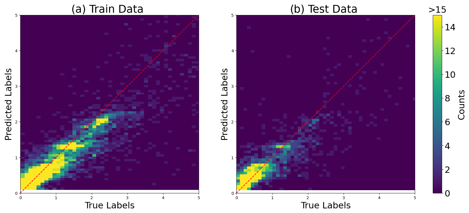
Figure 2 Heatmap of the correlation plot between measured (labels) and predicted data (targets) using DNN for (a) training data and (b) testing data in order to assess the model performance. The minimal difference observed between the training and testing errors serves as an indicator of the model's ability to avoid overfitting.

The prediction map of the DNN is presented in Fig. 3, while maps generated by kNN and random forests are provided in Appendix C (Figs. C1 and C2). Both the kNN and random forests showed artifacts, particularly in the equatorial Pacific and Atlantic oceans, similar to the map published by Lee et al. (2019). As stated by Lee et al. (2019), there is no standard means of quantifying uncertainty in kNN. In random forests, the variance or standard deviation of all the sub-output values for measuring the regression uncertainty is considered an uncertainty quantification method, but it is difficult to provide the uncertainty for an individual base learner (Lucas and Giles, 2016). Estimating the confidence of the predictions should be an important factor in deciding which model to use. On the other hand, uncertainty quantification in the DNN is an active field of research and has standardized methods. Nonetheless, kNNs and random forests are useful learning algorithms when computational resources are constrained and require an out-of-the-box solution.

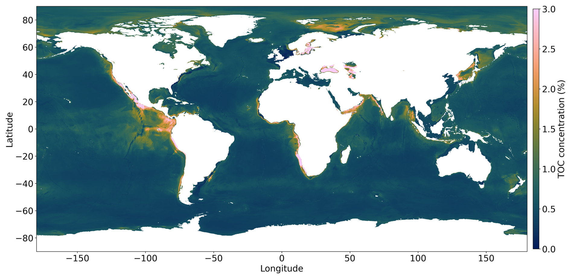
Figure 3 Global prediction map of the TOC concentration using a DNN. A higher TOC concentration is observed in the Arctic region and in upwelling areas located along the western continental margins of America and Africa, the equatorial Pacific, and the Arabian Sea.

We also tested a DNN model where the global ocean was not separated into shelf and deep-sea regions but treated as one entity. The resulting TOC map shows spurious features in the Pacific Ocean (Appendix E), similar to those found in previous predictions. This additional model shows that the separation of the ocean into shelf and deep-sea regions improves the model results.

Our DNN-based map of TOC concentrations (Fig. 3) shows similarities to maps previously published by Seiter et al. (2004) and Lee et al. (2019), who used geostatistical methods and a kNN model. All of the maps show elevated concentrations in the Arctic region and in upwelling areas located along the western continental margins of North America, South America, Africa, the equatorial Pacific, and the Arabian Sea. This pattern can be explained by elevated rates of marine primary and export production in upwelling regions delivering large fluxes of TOC to the seabed. The low TOC values in the open oceans are related to lower productivity and the large water depths limiting the TOC flux to the deep-sea floor. The predictions in Fig. 3 are also consistent with the early work on TOC distributions by Berner (1982) and Emerson and Hedges (1988), showing low TOC values in the open oceans and elevated values for upwelling regions and the Arctic region. The high TOC concentrations predicted for the Black Sea and Baltic Sea (Fig. 3) are probably related to the lack of oxygen in the bottom waters of these marginal seas that promotes TOC preservation (Hedges and Keil, 1995). The map published by Lee et al. (2019) shows several large areas in the open Pacific that have unusually high TOC concentrations. These patches are probably not realistic since they do not appear in other maps and are not consistent with our understanding of the TOC cycle. They may be artifacts generated by the kNN method and the sparse data coverage in these regions. Our new map avoids these artifacts and presents a pattern that corresponds better to our understanding of TOC accumulation on the seafloor for both the deep sea and the continental shelf, which were never modelled individually on previous maps.

We also produced a map of TOC stocks for the global ocean (Fig. 4). The TOC stocks were calculated using the global porosity grid provided by Martin et al. (2015) and a density of dry solids (d_s) of 2.6 g cm⁻³. We performed the calculation for the top 10 cm of the sediment column since our TOC data have been measured within this mixed surface layer. Moreover, the top 10 cm are the most vulnerable and dynamic part of the sedimentary TOC pool since they are subject to frequent biological and physical mixing processes (Song et al., 2022) and are affected by human interventions such as bottom trawling (Sala et al., 2021).

$$\begin{array}{}\text{(1)}& \begin{array}{rl}\text{TOC stock}& =(\mathrm{1}-\text{porosity})\times d_{\mathrm{s}}\\ & \times \text{TOC concentration}\times \text{10\hspace{0.17em}cm}\end{array}\end{array}$$

Figure 4 TOC stock map using the global porosity grid provided by Martin et al. (2015). The colour map is shown on a logarithmic scale.

The TOC stock is computed for global oceans and major seas (Flanders Marine Institute, 2021), considering both continental shelves and deep-sea regions within each ocean and sea (Table 2). Notably, the mean TOC concentration on continental shelves exhibits significant variability across regions. A visualization of the TOC stock in the oceans is provided in Appendix D.

Table 2 TOC stock in the continental shelf and deep-sea regions.

^* The total sums and the mean concentrations in the continental shelves include the Baltic Sea and the Caspian Sea. Without these regions, the total TOC stock in the continental shelves is 18.66 Pg, the area of the continental shelves is 25.42 ×10⁶ km², and the mean TOC concentration is 0.66 %.

According to our model, most the TOC stock can be found in the vast deep-sea basins of the Pacific, Indian, and Atlantic oceans, which is due to the large area of these basins (Table 2). The shelf region harbours 12.1 % of the global stock (Table 2, excluding the Baltic Sea and Caspian Sea), similar to the fraction previously derived by Atwood et al. (2020), who suggested that 11.5 % of the global TOC stock is located on the continental shelves. The global TOC stock derived from our model amounts to 155.8 Pg carbon for the 10 cm layer considered in our calculations (Table 2). This value is close to the global stock in the top 10 cm derived by reactive transport modelling (170 Pg carbon, LaRowe et al., 2020a). The other stock estimates were calculated by applying a range of sediment thicknesses. When normalized to 10 cm, the stock reported by Lee et al. (2019) amounts to 174 Pg carbon, while the stock derived by Atwood et al. (2020) amounts to 232 Pg carbon. The first stock estimate, which was based on expert knowledge and a limited database, corresponds to only 49 Pg carbon when normalized to 10 cm (Emerson and Hedges, 1988), which is lower than our estimate. Our new global stock assessment, hence, falls into the range of previous estimates.

According to our DNN model, the mean TOC concentration in continental shelf sediments, excluding the Baltic Sea and the Caspian Sea (0.70 %), is close to the concentration in deep-sea sediments (0.59 %, Table 2). This is a surprising result since the high marine productivity and low water depths on the shelf induce high TOC fluxes to the seabed that should result in elevated TOC concentrations in surface sediments. Moreover, large amounts of terrestrial particulate organic carbon (POC) produced by land plants are deposited in shelf sediments (Burdige, 2005), which should further increase TOC concentrations in these deposits. However, TOC concentrations in shelf surface sediments are diminished by a number of factors: (i) frequent biological and physical reworking that accelerates TOC degradation processes (Song et al., 2022), (ii) dilution of TOC by inorganic material (clay, silt, and sand) in delta deposits and other shelf regions with high sedimentation rates (Berner, 1982), (iii) strong bottom currents that inhibit sediment deposition such that large shelf areas are covered by relict coarse-grained sediments that were deposited in the geological past and that do not contain significant amounts of TOC (Emery, 1968), and (iv) frequent bottom trawling that exposes sedimentary TOC to oxygen and accelerates TOC degradation (Atwood et al., 2020). According to our DNN model, these factors could potentially decrease TOC concentrations in shelf sediments to such a degree that they attain mean values that are close to those observed in deep-sea sediments (Table 2). It should, however, be noted that most TOC burial occurs on the shelf, where sedimentation rates are elevated due to the deposition of riverine particles (Bradley and Arndt, 2022).

A method based on cooperative game theory (SHAP, SHapley Additive exPlanations) is used to analyse our results further and identify features that have a large effect on the predicted distribution of TOC concentrations (Lundberg and Lee, 2017). The higher the SHAP value for a feature, the more important the feature is for the predictions of that particular model. According to our model analysis, the total oxygen uptake feature (Jørgensen et al., 2022) has the largest effect (SHAP value) on predicted TOC concentrations in shelf sediments, while the global porosity grid (Martin et al., 2015) was the most important feature for deep-sea sediments. It should, however, be noted that the feature importance ranking is only valid for our specific model set-up and might not be representative of the real world. Model interpretability and feature importance ranking are discussed further in Appendix F.

To guide future sampling, a new information gain map is provided (Fig. 5). It identifies the regions that should be explored in order to improve the current model predictions. Some of the main takeaways from the information gain map are that (i) regions with high information gain are found in parts of the equatorial Pacific Ocean, in Zealandia, and around Papua New Guinea. These regions are less explored geographically, and hence the model is not trained with the features in this region. (ii) The continental slopes on the western coast of North America, in the east of Iceland, and in parts of the eastern coast of Africa have a higher information gain, though they have more measurements. This could be due to the steep slopes and rough topography in these regions that may induce a high spatial heterogeneity in TOC values that is not yet resolved by the model. (iii) Though the Southern Ocean is not well-explored, regions with higher information gain are only found with relatively steep terrain, such as areas located close to islands and ocean ridges. These examples show that an abundance of measurements does not necessarily correspond to lower information gain and vice versa. Information gain depends not only on the geographical proximity of measurements, but also on their proximity in the parameter space and the congruence of the measurements made there. Including measurements from a region of higher information gain should lead to higher model knowledge, and hence this is more valuable compared to regions of low information gain. An experiment showing this is presented in Appendix B.

Figure 5 The information gain map serves as a guide for determining optimal sampling locations, i.e. those with high information gain values. The colour scheme highlights the high information gain regions with brighter colours. Information gain does not have any units and is non-negative – [0,inf).

5 Conclusions

The comparison between different modelling approaches, including DNNs, kNNs, and random forests, highlights the effectiveness of each method in predicting TOC concentrations. While kNN and random forest models exhibit higher correlation coefficients and overall performance in the training dataset, the DNN outperforms them in testing data performance. This suggests a potential overfitting issue with the kNN and random forest models, where they may have become specialized in learning the training data. Nonetheless, these algorithms remain useful, especially when computational resources are limited.

Our DNN-based map of TOC concentrations shows elevated values in specific regions such as the Arctic and upwelling areas along continental margins. These patterns are consistent with known processes of marine primary and export production. Notably, our model that treats the shelf and deep-sea regions as separate entities captures their individual dynamics with higher accuracy and yields a better global map of TOC concentrations than a model version that simulates the entire ocean as one continuous system. It specifically avoids artifacts like unrealistically high TOC concentrations in open-ocean regions with poor data coverage that have also been encountered in previous kNN and forest models. The computed TOC stock for global oceans and major seas provides valuable insights into the distribution and magnitude of TOC storage. Despite significant variability in the mean TOC concentration across continental shelves, our model confirms that the majority of the TOC stock is found in deep-sea basins. Surprisingly, mean TOC concentrations in continental shelves are close to those in deep-sea sediments, suggesting complex processes at play that diminish TOC concentrations in shelf sediments.

The analysis of information gain highlights regions with sparse or contradicting measurements and higher uncertainty, providing guidance for future sampling efforts. It reveals that the abundance of measurements does not necessarily correspond to lower uncertainty, emphasizing the importance of considering both geographical proximity and parameter space proximity in sampling strategies.

In conclusion, our study contributes to a better understanding of global TOC distributions and stocks, shedding light on the complex interplay between biological, physical, and geological processes in marine sedimentary environments. The insights gained from our modelling approach can inform future research and management efforts aimed at preserving and managing marine carbon sinks.

Appendix A: Feature list

File names adhere to the naming conventions discussed below. The naming structure is partitioned by underscores and periods in the following order: the interface to which the gridded values refer, the quantity of values contained within the grid, the units and reference values or units (e.g. metres below sea level), the data source, the statistic calculated (if applicable), the grid pitch, and the file extension.

SS	Sea surface–atmosphere interface (may also be the average of the entire water column)
SF	Seafloor–water interface (may also be denoted by GL – ground level)
(r50 km) – raw feature and feature averaged at a 50 km radius
The units referenced are as follows.
KGM3	Kilograms per cubic metre
MS	Metres per second
KM	Kilometres
M_ASL	Metres above sea level (i.e. metres referenced to the sea level)
MWM2	Milliwatt per square metre
TGCYR	Teragrams of carbon per year
TGYR	Teragrams per year
MA	Mega-annum
M	Metres
MGCM2	Milligrams of carbon per square metre
DEG	Degrees
S	Seconds

Most of the features presented below were collected by Lee et al. (2020) and Phrampus et al. (2019). The new datasets, including the additions from this work, are available at https://doi.org/10.5281/zenodo.11186224 (Parameswaran et al., 2024b).

National Geophysical Data Center (2006)National Geophysical Data Center (2006)National Geophysical Data Center (2006)National Geophysical Data Center (2006)Ludwig et al. (2011)Ludwig et al. (2011)Ludwig et al. (2011)Ludwig et al. (2011)Ludwig et al. (2011)Whittaker et al. (2013)Hart-Davis et al. (2021)Hart-Davis et al. (2021)NASA (2014)NASA (2014)Becker et al. (2014)National Geophysical Data Center (2006)Martin et al. (2015)Kim and Wessel (2011)Boyer et al. (2013)National Geophysical Data Center (2006)The HYCOM+NCODA Ocean Reanalysis (2014)National Geophysical Data Center (1976)Joint Panel on Oceanographic Tables and Standards (1991)Boyer et al. (2013)Boyer et al. (2013)Boyer et al. (2013)Boyer et al. (2013)Boyer et al. (2013)Boyer et al. (2013)Boyer et al. (2013)Boyer et al. (2013)Pavlis et al. (2008)Lee et al. (2019)Wei et al. (2010)NASA (2014)Lee et al. (2020)NASA (2011)Pavlis et al. (2008)Goyet et al. (2000)NASA (2014)The HYCOM+NCODA Ocean Reanalysis (2014)NASA (2011)Jørgensen et al. (2022)Garlan et al. (2018)Garlan et al. (2018)Garlan et al. (2018)Garlan et al. (2018)Garlan et al. (2018)Garlan et al. (2018)Garlan et al. (2018)

Table A1 Feature list with the descriptions and references used as input for all of the models in the paper.

Appendix B: Information gain

In this paper, KL divergence, also known as information gain or relative entropy, has been used to quantify model uncertainty. As Rényi (1961) pointed out, in the absence of observational information, the amount of information can be taken to be numerically equal to the amount of uncertainty concerning the model prediction. The mathematical derivation of KL divergence against the theoretical background of information theory (Shannon, 1948) is presented below. The information entropy of a random variable X with a probability distribution P is represented as

$$\begin{array}{}\text{(B1)}& H\left(P\right)=-\sum _{i}P\left({\mathit{x}}_i\right)\log P\left({\mathit{x}}_i\right).\end{array}$$

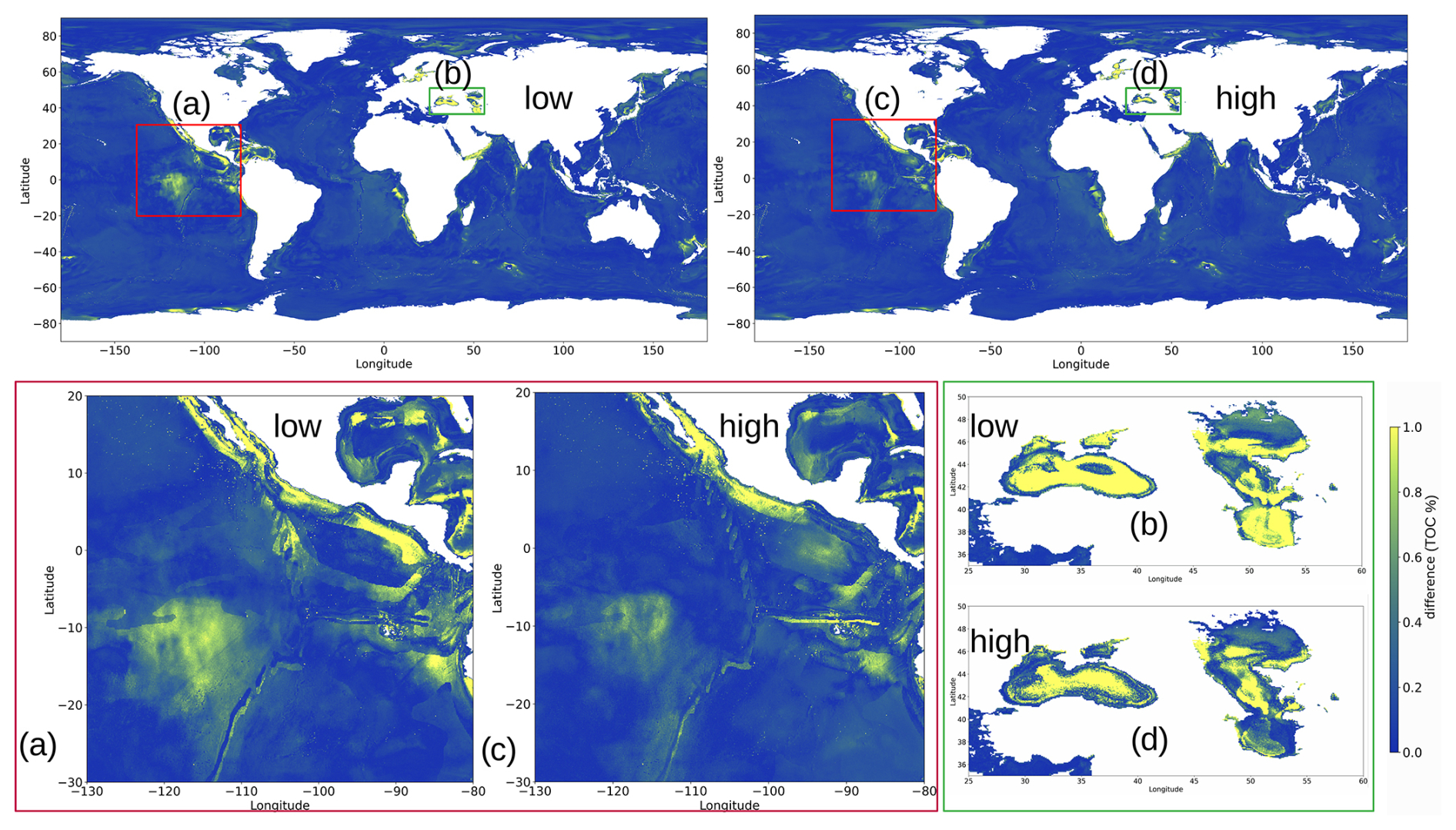
Figure B1 Top left: difference in the prediction of the TOC concentration between $\mathit{\varphi }(\mathit{x},\mathbf{W},\mathit{b})$ and ${\mathit{\varphi }}_{\mathrm{wh}+\mathrm{low}\mathrm{\_}\mathrm{ig}}(\mathit{x},\mathbf{W},\mathit{b}{)}_{\mathrm{2}}$. Top right: difference in the prediction of the TOC concentration between $\mathit{\varphi }(\mathit{x},\mathbf{W},\mathit{b})$ and ${\mathit{\varphi }}_{\mathrm{wh}+\mathrm{high}\mathrm{\_}\mathrm{ig}}(\mathit{x},\mathbf{W},\mathit{b}{)}_{\mathrm{2}}$. Brighter colours (shades of yellow) show higher differences, and darker colours (shades of blue) show lower differences. Bottom left (red box): zoomed-in version of the equatorial Pacific region in panels (a) and (c). Bottom right (green box): zoomed-in versions of the Caspian and Black seas in panels (b) and (d).

The Shannon (1948) definition of entropy determines the minimum channel capacity required to reliably transmit the information as encoded binary digits. Usually, the true distribution P(X) denotes observed data, measurements, or an exact probability distribution. Here, P(X) is constructed using a normal distribution with a mean value equal to Monte Carlo dropout prediction and a standard deviation of 0.05 TOC %, which arises from both technical handling and the precision of the weighting tool (Pape et al., 2020). The predicted distribution Q(X) is derived from the Monte Carlo dropout prediction ensemble. The measure Q(X) typically represents a theoretical framework, a model, a description, or an approximation of P(X). The cross-entropy between P(X) and Q(X) measures the average number of binary digits to represent an event from P(X) by Q(X). It is represented as

$$\begin{array}{}\text{(B2)}& H(P,Q)=-\sum _{i}P\left({\mathit{x}}_i\right)\log Q\left({\mathit{x}}_i\right).\end{array}$$

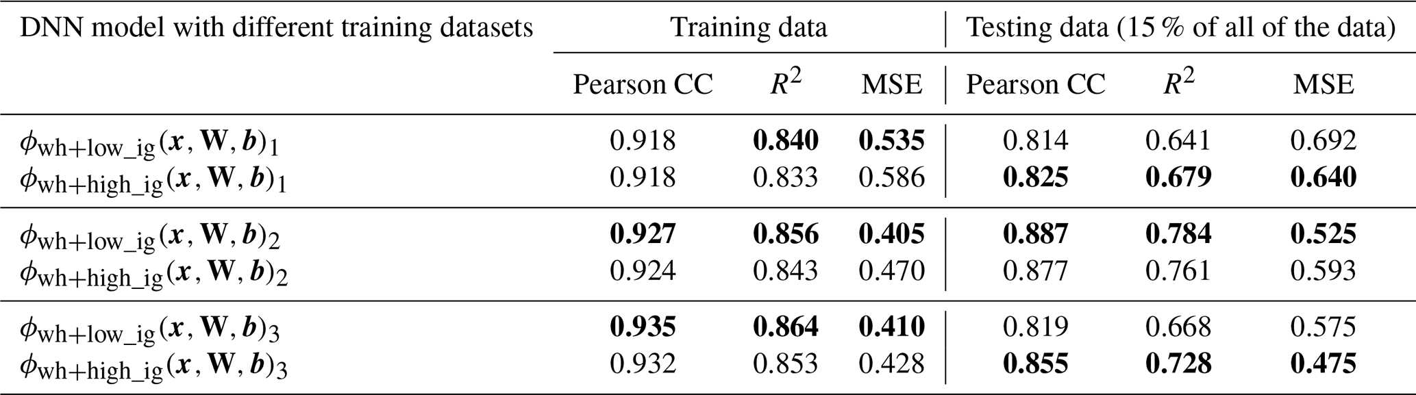
Table B1 Performance metrics of models trained on different subsets of data based on information gain for different splits of data (seeds): Pearson CC, R², and MSE for predicted values vs. observed labels for the training and testing data. The train:test data ratio is 85:15. The better-performing dataset, based on the metric, is highlighted in bold. It shows that the performance on the test dataset, or the generalisation is mostly higher when using the dataset with higher information gain.

The information gain that measures the difference between the cross-entropy (Eq. B2) and the entropy (Eq. B1) is represented as D_KL(P‖Q).

$$\begin{array}{}\text{(B3)}& \begin{array}{rl}{D}_{\text{KL}}(P\Vert Q)& =H(P,Q)-H\left(P\right)\\ & =\sum _{i}P\left({\mathit{x}}_i\right)\log \left({\displaystyle \frac{P\left({\mathit{x}}_i\right)}{Q\left({\mathit{x}}_i\right)}}\right)\end{array}\end{array}$$

D_KL(P‖Q) is always non-negative and remains well-defined for continuous distributions. To obtain the continuous distribution for the predicted distribution Q(X), the prediction ensemble is binned into histograms to obtain an approximate probability density function (PDF). This PDF is then modelled using curve-fitting techniques typically fitted to a Gaussian distribution (Algorithm G2). D_KL(P‖Q) is calculated globally for each prediction and plotted on the information gain map.

In supervised machine learning, a model's predictive performance is usually determined by withholding a test dataset during the training phase and comparing the final model outputs to these known values. Such a procedure is not possible when evaluating the performance of information gain: firstly, the concept of a ground truth for the information gain values does not exist. Secondly, we aim to measure the effect that data point selection guided by information gain has on the model output, not the information gain itself. Thus, in order to explore the effect that information gain has on data sampling and model refinement, we devised the following experiment: a DNN model with the same parameters as the original one was trained while withholding one-third of the original training dataset: ${\mathit{\varphi }}_{\mathrm{wh}}(\mathit{x},\mathbf{W},\mathit{b})$. Afterwards, this model was used to calculate the information gain for each point in the withheld data. These additional data points were sorted according to their information gain values and divided into two subsets of equal size. Each of these subsets was used along with the initial two-thirds to train two new DNN models: one with added high information gain data points (${\mathit{\varphi }}_{\mathrm{wh}+\mathrm{high}\mathrm{\_}\mathrm{ig}}(\mathit{x},\mathbf{W},\mathit{b})$) and one with added low information gain data points (${\mathit{\varphi }}_{\mathrm{wh}+\mathrm{low}\mathrm{\_}\mathrm{ig}}(\mathit{x},\mathbf{W},\mathit{b})$). To validate the entirety of the training data, the process was repeated two more times, withholding a different third of the dataset each time.

In two of the three executions, the (test) performance of ${\mathit{\varphi }}_{\mathrm{wh}+\mathrm{high}\mathrm{\_}\mathrm{ig}}(\mathit{x},\mathbf{W},\mathit{b})$ was superior to that of ${\mathit{\varphi }}_{\mathrm{wh}+\mathrm{low}\mathrm{\_}\mathrm{ig}}(\mathit{x},\mathbf{W},\mathit{b})$ (Table B1). While the difference in performance from the different data subsets might be small in magnitude, the selection of high information gain points also has a positive effect on the structure of the global inference patterns: in Fig. B1 we took the prediction maps for both models of the worst-performing data subset, ${\mathit{\varphi }}_{\mathrm{wh}+\mathrm{high}\mathrm{\_}\mathrm{ig}}(\mathit{x},\mathbf{W},\mathit{b}{)}_{\mathrm{2}}$ and ${\mathit{\varphi }}_{\mathrm{wh}+\mathrm{low}\mathrm{\_}\mathrm{ig}}(\mathit{x},\mathbf{W},\mathit{b}{)}_{\mathrm{2}}$, and calculated the absolute difference between them and the inference map of the original model $\mathit{\varphi }(\mathit{x},\mathbf{W},\mathit{b})$ in Fig. 3. Regardless of the performance metrics, the high information gain model resembles the output of the original model more closely than the low information gain model.

Appendix C: Comparison of the methods

One of the drawbacks of using DNN is the number of hyperparameters that needs to be tuned. The number of layers and the nodes in each layer were decided using a trial-and-error method starting with the simplest configuration of three layers of eight neurons. The model complexity was increased till the validation and training performance were comparable, thus avoiding overfitting while still getting relatively good performance in the test dataset. The initial learning rate was chosen based on the model convergence. The DNN model had 10 layers of 128 nodes each with a learning rate of 0.01. The batch size, decided based on the amount of data, was set to 500 and was also chosen based on model convergence. On the other hand, the parameters that were tuned in the random forest algorithm and kNNs were the number of trees in the forest (controlled by the number of estimators in sklearn) and the number of neighbours, respectively. They are tuned using the performance metrics for 1–50 neighbours for kNN. The number of estimators is 10, 20, 30, …, 100 for random forests.

Though it is difficult to tune the DNN model, Table 1 highlights superior performance in the training dataset for kNNs and random forests, while their test performance or generalization capability lags behind that of DNNs. Figures C1 and C2 show artifacts of the global predictions from kNNs and random forests, particularly in the equatorial Pacific and Atlantic oceans.

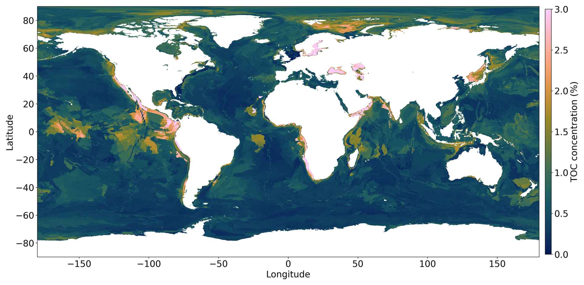
Figure C1 Global prediction map of TOC concentrations using a k-nearest neighbour algorithm, with the five nearest neighbours in the continental shelves and the four nearest neighbours in the deep sea. Spurious patches are observed in the equatorial Pacific Ocean and in the Atlantic Ocean.

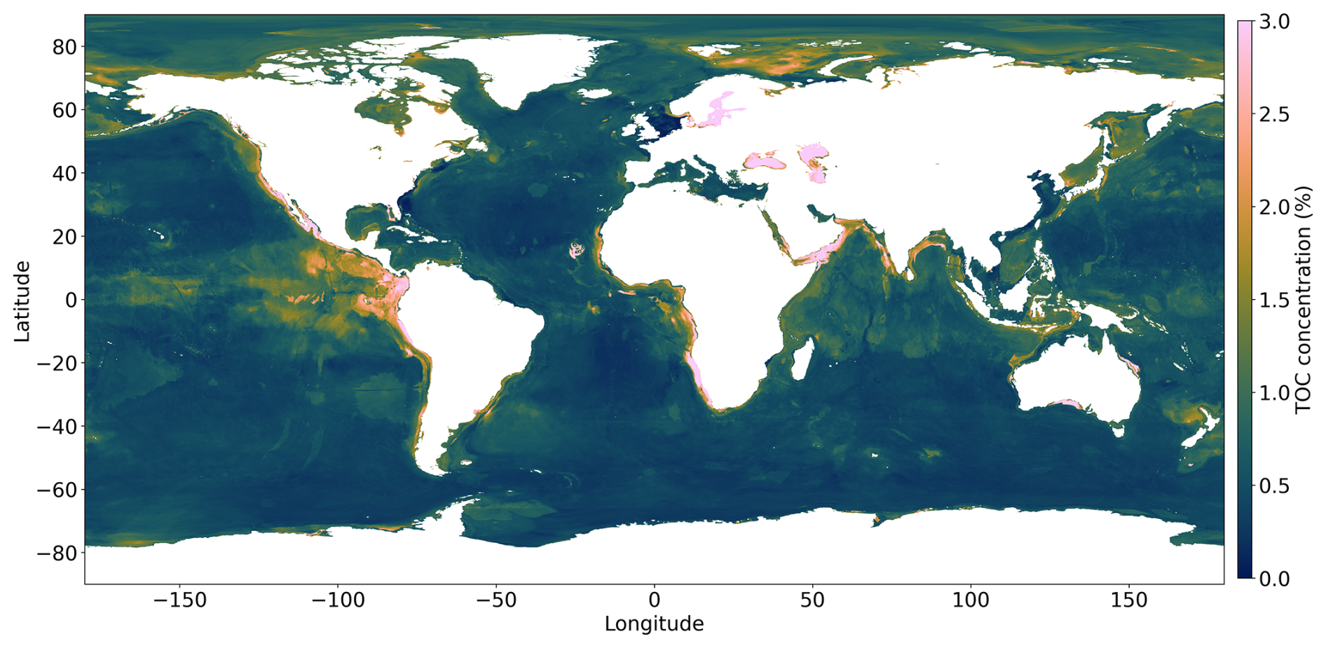
Figure C2 Global prediction map of TOC concentrations using a random forest algorithm with 100 estimators. Spurious patches are observed in the Atlantic Ocean and the Bay of Bengal.

Appendix D: TOC stock in different marine regions

Table 2 breaks down how much TOC stock is found in different parts of the ocean. Each region is listed, showing how much TOC is there. Here we show a visualization of the different regions in Fig. D1.

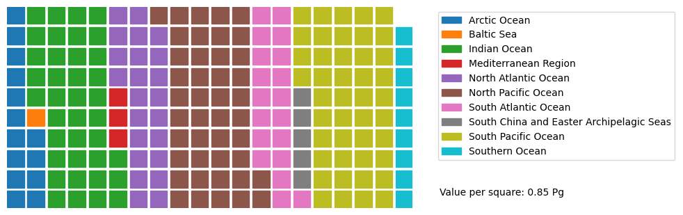
In Fig. D2, we use a waffle chart to make it easier to see how the TOC is split among these regions. It is like dividing a pie into slices, but here we use squares. With a total of about 156 Pg of TOC worldwide, the South Pacific Ocean gets the biggest share, while the Baltic Sea gets the smallest.

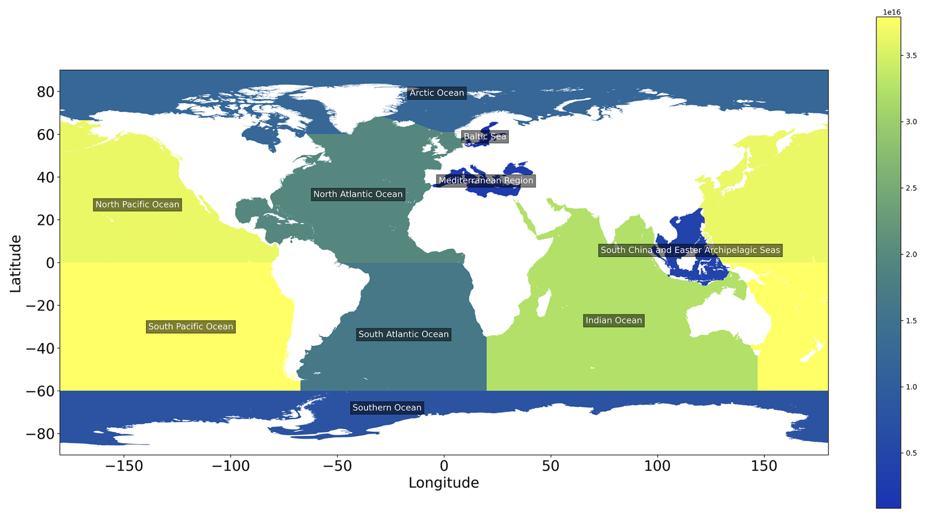
Figure D1 TOC stocks in different oceans.

Figure D2 TOC stocks in different oceans: waffle chart.

Appendix E: DNN model run without separation of deep-sea and shelf environments

Here, we test a DNN model where the global ocean was not separated into shelf and deep-ocean regions but treated as one entity. The resulting TOC map shows spurious features in the Pacific Ocean, similar to those that occur in the map published by Lee et al. (2019). These results underscore the importance of separating shelf and deep-ocean regions in order to achieve more accurate and realistic model outcomes.

Figure E1 TOC concentration map when the DNN model was not separated into shelf and deep-ocean regions. We see unrealistic TOC concentrations, especially in the Pacific Ocean.

Appendix F: Model interpretability using SHAP values

Explaining and understanding why a model makes a certain prediction is as crucial as accuracy and uncertainty in the predictions. This becomes particularly challenging in high-dimensional spaces, where interpreting complex models can be more intricate compared to simpler yet less accurate models. Lundberg and Lee (2017) proposed SHAP as a unified framework for interpreting predictions. SHAP assigns importance values to each feature for a particular prediction, providing a comprehensive understanding of the model's decision-making process. In our supervised learning model f trained on features $X\in \mathcal{X}\subseteq {\mathbb{R}}^d$ to predict outcomes $Y\in \mathcal{Y}\subseteq \mathbb{R}$, SHAP, a feature attribution method, considers the model predictions to be decomposed as a sum $f\left(x\right)={\mathit{\varphi }}_{\mathrm{0}}+{\sum }_{j=\mathrm{1}}^d\mathit{\varphi }(j,x)$, where ϕ₀ is the baseline expectation (i.e. ϕ₀=𝔼[f(x)]) and ϕ(j,x) denotes the Shapley value of feature j at point x.

In our analysis, we aim to simplify the interpretation process by presenting the average importance of features across all of the predictions, from the deep sea to the continental shelves. All of the effects describe the behaviour of the model and are not necessarily causal in the real world.

The summary plot in Figs. F1 and F2 combines the feature importance with feature effects. The summary plot displays Shapley values representing the impact of features on predictions. Each point represents a Shapley value for a feature and an instance. The y axis position indicates the feature, while the x axis position corresponds to the Shapley value. Feature values are represented by colours ranging from low (blue) to high (red). To visualize feature importance, points are spread along the y axis to reveal the distribution of Shapley values per feature. The features are ordered based on their importance, determined by the mean absolute Shapley values across all of the predictions. The Shapley value is expressed in the same units as the TOC concentration. This indicates the extent to which a specific feature value influences the TOC concentration and whether it drives it towards higher or lower values.

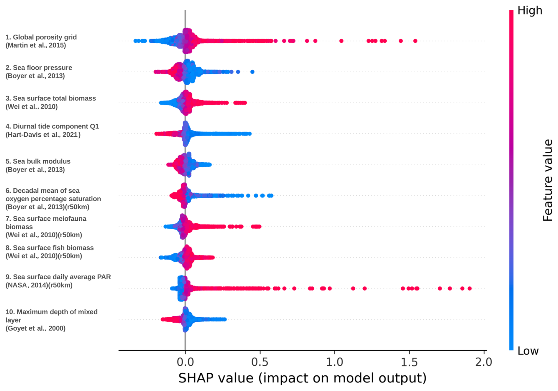
Figure F1 Summary plot of Shapley values of the deep-sea DNN model. The global porosity grid (Martin et al., 2015) has the highest feature importance. Regions with high porosity lead to higher TOC concentrations and vice versa. In the mechanistic model of Bradley and Arndt (2022), porosity is positively correlated with the organic carbon flux through a specific depth. The biological features that include total biomass, meiofauna, fish biomass in the sea surface (Wei et al., 2010), oxygen concentration in bottom waters (Boyer et al., 2013), and daily average PAR (NASA, 2014) show that higher biomass or marine productivity leads to higher TOC concentrations, as expected. On the other hand, higher oxygen saturation leads to oxic conditions, resulting in the oxidation of the organic carbon and hence a lower TOC concentration. The other features which dominate are the physical oceanographic features, where higher feature values result in lower TOC concentrations, such as tidal features (Q1 loading) (Hart-Davis et al., 2021), sea bulk modulus (Boyer et al., 2013), and seafloor pressure (Boyer et al., 2013).

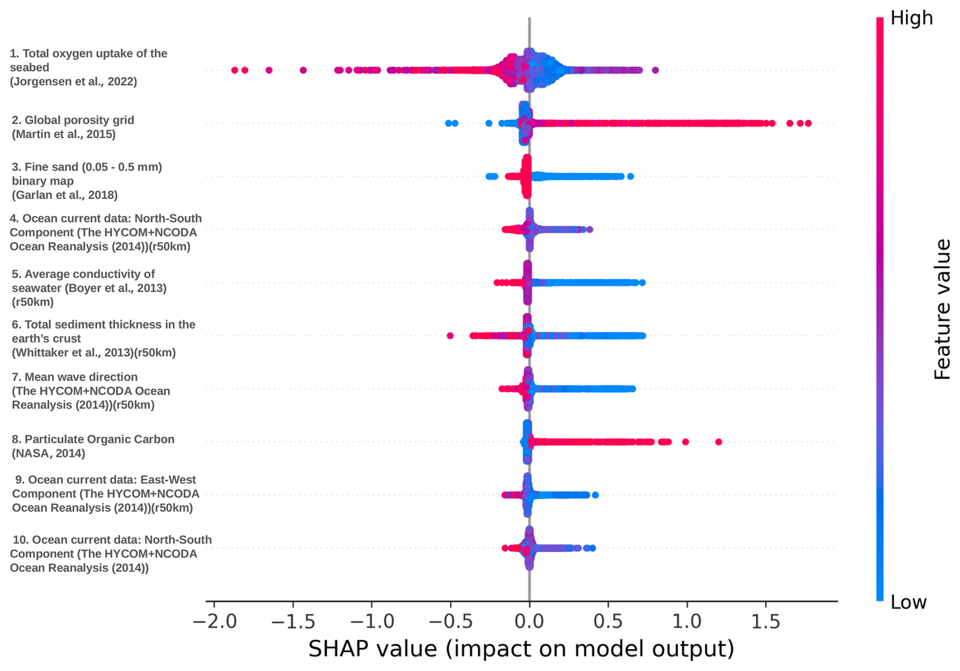
Figure F2 Summary plot of Shapley values of the continental shelf DNN model. The total oxygen uptake (Jørgensen et al., 2022) of the seabed has the highest feature importance, with regions of higher oxygen uptake resulting in lower TOC concentrations and denoting oxic conditions. Regions with higher porosity (Martin et al., 2015) result in higher TOC concentrations, while regions with lower porosity result in lower TOC concentrations but with less impact. The lithology map is a binary map. Regions with fine sand, with grain sizes between 0.05 and 0.5 mm (1 mm being the higher feature value), have low TOC concentrations. Higher sediment thicknesses in Earth's crust lead to lower TOC concentrations because of dilution (Berner, 1982). The bottom current components, north–south and east–west, result in reduced TOC concentrations due to higher resuspension of sediments, the inhibition of sedimentation, and burial of organic carbon. Higher average seawater conductivity results in lower TOC concentrations. Higher particulate organic carbon (POC) in the water column has a positive impact on the TOC concentrations, as expected. It can be seen that the feature importance is not as clearly defined as in the deep ocean (as the high (red) and low (blue) feature values are mixed) because of the complex dynamics on continental shelves.

Appendix G: Algorithms

Algorithm G1 DNN training with batch normalization and dropout, including Monte Carlo dropout for inference.

Require:

Labelled dataset $D=\mathit{\left\{}\right(x_{\mathrm{1}},y_{\mathrm{1}}),(x_{\mathrm{2}},y_{\mathrm{2}}),\mathrm{\dots },(x_N,y_N\left)\mathit{\right\}}$

x_i: feature vector for the ith label

y_i: corresponding TOC %

1:

Input: feature vector x_j

2:

Output: predicted TOC % predicted% for x_j

3:

Method: construct a neural network with 10 layers and 128 nodes per layer: $\mathit{\varphi }(\mathit{x},\mathbf{W},\mathit{b})$

4:

Apply batch normalization and dropout to each layer.

5:

Initialize optimizer (e.g. Adam) with appropriate learning rate and parameters.

6:

Initialize loss function (e.g. mean squared error) for regression.

7:

Train the neural network with D for 1000 epochs:

8:

for epoch=1 to num_epochs do

9:

Randomly shuffle the training dataset..

10:

for (x_i,y_i) in D do

11:

Forward pass: compute predictions $\widehat{y_i}=\mathit{\varphi }({\mathit{x}}_i,\mathbf{W},\mathit{b})$.

12:

Compute target loss: ${\text{loss}}_{\text{target}}=\text{MSE}(y_i,\widehat{y_i})$.

13:

Back-propagation: update weights and biases using optimizer, with loss_target as the cost function.

14:

end for

15:

end for

16:

Set dropout to active during inference

17:

Perform Monte Carlo dropout for M forward runs:

18:

${\widehat{y}}_j^{\text{ensemble}}=\mathit{\varphi }({\mathit{x}}_j,\mathbf{W},\mathit{b},{\text{dropout\_mask}}_T)$

19:

Predicted TOC %, $\widehat{y_j}$ for ${\mathit{x}}_j=\frac{\mathrm{1}}{M}{\sum }_{m=\mathrm{1}}^M{\widehat{y}}_j^{\text{ensemble}}$

Algorithm G2 Calculating information gain for the predictions.

Require:

Monte Carlo dropout prediction ensemble, ${\widehat{y}}^{\text{ensemble}}$, for each grid cell

1:

for each grid cell do

2:

Fit a Gaussian probability density function Q_j(y) for ${\widehat{y}}_j^{\text{ensemble}}$ using histograms and curve fitting algorithm.

3:

Generate original distribution P_j(y) with mean $\widehat{y_j}$ and standard deviation 0.05 (sampling error).

4:

Calculate Kullback–Leibler divergence:

$D_{\text{KL}}(P_j\Vert Q_j)={\sum }_i{P}_j\left({\mathit{y}}_i\right)\log \left(\frac{P_j\left({\mathit{y}}_i\right)}{Q_j\left({\mathit{y}}_i\right)}\right)$

5:

end for