LM4-SHARC v1.0: resolving the catchment-scale soil–hillslope aquifer–river continuum for the GFDL Earth system modeling framework

Catchment-scale representation of the groundwater and its interaction with other parts of the hydrologic cycle is crucial for accurately depicting the land water–energy balance in Earth system models (ESMs). Despite existing efforts to describe the groundwater in the land component of ESMs, most ESMs still need a prognostic framework for describing catchment-scale groundwater based on its emergent properties to understand the implications for the broader Earth system. To fill this gap, we developed a new parameterization scheme to resolve the groundwater and its two-way interactions with the unsaturated soil and stream at the catchment scale. We implemented this new parameterization scheme (SHARC, or the soil–hillslope aquifer–river continuum) in the Geophysical Fluid Dynamics Laboratory (GFDL) land model (i.e., LM4-SHARC) and evaluated its performance. By bridging the gap between hydraulic groundwater theory and ESM land hydrology, the new LM4-SHARC provides a path to learning groundwater emergent properties from available streamflow data (i.e., recession analysis), enhancing the representation of subgrid variability in water–energy states induced by the groundwater. LM4-SHARC has been applied to the Providence headwater catchment at Southern Sierra, NV, and tested against in situ observations. We found that LM4-SHARC leads to noticeable improvements in the representation of key hydrologic variables such as streamflow, near-surface soil moisture, and soil temperature. In addition to enhancing the representation of the water and energy balance, our analysis showed that accounting for groundwater convergence can induce a more significant hydrologic contrast, with higher sensitivity of soil water storage to groundwater properties in the riparian zone. Our findings indicate the feasibility of incorporating two-way interactions among groundwater, unsaturated soil, and streams into the hydrological components of ESMs and show a further need to explore the implications of these interactions in the context of Earth system dynamics.

1 Introduction

The significance of understanding the relationship between the hydrologic cycle and climate variability has been increasingly recognized in a warming climate (Milly et al., 2008). As a major component of the terrestrial water cycle, groundwater (i.e., water in saturated zones beneath the land surface) plays a pivotal role in developing the surface thermal energy and moisture dynamics and the land–atmosphere coupling by regulating how the water and thermal energy are stored and transported across the landscape (Andreae et al., 2002; Mu et al., 2011; McCabe et al., 2008; Gentine et al., 2019; Fan, 2015). The effects of the groundwater state (e.g., storage) on the water–energy balance at the land surface have been discussed in several studies based on an explicitly treated groundwater scheme (Miguez-Macho et al., 2007; Liang et al., 2003; Yeh and Eltahir, 2005; Zeng et al., 2016; Maxwell et al., 2011; Maxwell and Kollet, 2008). The studies commonly found higher sensitivity of the surface energy balance to groundwater storage if the water table is shallow (e.g., the water table depth is less than 5 m).

However, many Earth system models (ESMs) only represent the top few meters of soil, and most, if not all, ignore two-way interactions between the groundwater and other components of the hydrologic cycle. In particular, ESMs lack proper land surface scheme(s) to represent the two-way interactions between the groundwater and the stream/river while conserving the hydraulic continuity between them. In most cases, the river routing module implemented in the ESMs exists mainly for traditional purposes (e.g., linking precipitation-induced runoff to the ocean) without the ability to consider the groundwater variations driven by the horizontal hydraulic gradients between the stream and the groundwater (Li et al., 2013; De Rosnay et al., 2002; Lawrence et al., 2011, 2019; Miguez-Macho and Fan, 2012; Best et al., 2011; Takata et al., 2003).

Furthermore, the resolution of climate-/water-related information provided by the current ESMs is too low to characterize hydrological extremes and address the stakeholders' need to evaluate potential impact of future climate change. Even atmosphere–land water information produced at a resolution of 0.25° (Delworth et al., 2020) – the highest resolution in ESMs – is still not sufficiently fine to generate fine-scale data for decision-making. The land components of ESMs generate the streamflow estimates only at a grid scale (typically ranging from 0.5 to 1.0°) (Oleson et al., 2013; Miguez-Macho et al., 2007; Fan et al., 2007; Pappenberger et al., 2012; Campoy et al., 2013), and since such coarse-resolution streamflow data, for example, is not suitable for directly locating hydrologic events at a fine scale, even in the case of extremes (e.g., flooding), the scale mismatch (between the stakeholders and ESMs) could reduce the usability of the ESM-derived projections. Another challenge lies in the high degree of land heterogeneity with respect to soil and topographic characteristics, which needs to be resolved at the ESM grid scale. Considering the significant impacts of the fine-scale soil/topographic properties on the hydrologic processes, the two-way interactions between the groundwater and the rest of the hydrologic cycle must be parameterized at the subgrid scale (e.g., catchment) to adequately represent the subgrid variability in hydrologic states and to show its implications for the broader Earth system processes and interactions (Gleeson et al., 2020; Xu et al., 2023; Maxwell and Kollet, 2008; Pokhrel et al., 2013).

Catchments provide an appropriate scale to properly capture such subgrid spatial heterogeneity and its effect on the interactions among the hydrological cycle components (Clark et al., 2015; Fan et al., 2019; Blyth et al., 2021). This is mainly due to the suitability of the catchment scale in describing the topographically driven flow characteristics of water and other major fluxes (e.g., thermal energy) caused by water transport. In fact, catchments are sometimes considered hydrologic spatial units (or response units), where the theoretical conceptualization of surface and subsurface water transport can be tested with readily available observational data, such as streamflow measurements (Sivapalan, 2006; Troch et al., 2013; Kirchner, 2009). Over the past decades, a strong effort has been made to depict the hydraulically based interactions among the distinct flow domains at the hillslope and catchment scales (Kollet and Maxwell, 2006; Niu et al., 2011; Shen and Phanikumar, 2010; Gochis, 2021). This effort mainly aimed to represent the water–energy coupled balance while considering the time-dependent nonlinear relationship between water states and fluxes based on Darcian flow (Clark et al., 2015; Fan et al., 2019).

However, when specifically targeting the representation of the groundwater and its interactions with the overlying soil and the stream/river, the spatial heterogeneity of groundwater properties (e.g., diffusivity or effective (drainable) porosity) remains a significant challenge for enhancing the predictability of terrestrial water storage and exchange fluxes (Clark et al., 2009; Jing et al., 2019). Notably, accurate description of groundwater properties/processes at the catchment-scale is crucial because the hydrologic convergence (to the riparian zone) and divergence (from the hilltops) by the groundwater movement significantly affects the catchments' water and energy dynamics (Fan, 2015; Miguez-Macho and Fan, 2012; Chen and Hu, 2004; Maxwell et al., 2007). Even in previous studies that captured the interactions among the soil, groundwater, and streams, the properties of the groundwater were treated as constant and not as emergent and were treated as dynamic properties as the result of transient groundwater storage affected by the climate (e.g., precipitation) or human activities (e.g., land use change or groundwater pumping) (Li and Ameli, 2022; Bart and Hope, 2014; Jachens et al., 2020b; Hong and Mohanty, 2023a; Trotter et al., 2024). For example, these studies empirically fit coefficients to a storage–discharge function (e.g., bucket model) or to a predefined soil properties dataset to parameterize the groundwater domains (Zeng et al., 2016; Gochis, 2021; Newman et al., 2014; Kollet and Maxwell, 2008; Leung et al., 2011; Li and Ameli, 2022). Thus, a theoretical approach to capture the dynamic, emergent properties of the catchment-scale groundwater has largely been absent in these efforts.

The Dupuit–Forchheimer (DF) approximation allows the incorporation of the catchment-scale groundwater into ESMs and accounts for emergent properties/processes that shape the interactions with the unsaturated soil and the stream (Dupuit, 1863; Forchheimer, 1986). According to the DF approximation, heterogeneity in groundwater properties can be represented by effective parameters reflecting the combined effects of the groundwater property variability on fluxes (e.g., baseflow), assuming that the lateral groundwater discharge is from the homogeneous/isotropic (or systemically defined) groundwater (Rupp and Selker, 2006; Strack, 1995; Beven and Kirkby, 1979). The DF approximation is especially relevant, as the heterogeneity of groundwater properties that are not representable below a model-specific resolution can be considered one of the challenges for the accuracy of modeled data (Baroni et al., 2019; Maxwell et al., 2015; Niu et al., 2011; Bisht et al., 2017). The DF approximation is derived by recasting the analytical solution of the Boussinesq equation (Boussinesq, 1903) into the power law streamflow recession model by Brutsaert and Nieber (1977). This method of streamflow recession analysis provides a theoretical basis for estimating the effective groundwater properties on a catchment scale using (relatively readily) available streamflow observations (Tashie et al., 2021; Hong and Mohanty, 2023a; Vannier et al., 2014; Brutsaert and Lopez, 1998; Troch et al., 1993; Xu et al., 2018).

The catchment-scale processes can be resolved at the ESM grid scale via approaches to the subgrid model structure such as HydroBlocks (Chaney et al., 2016, 2018). The hierarchical multivariate clustering (HMC) approach, as implemented in LM4-HydroBlocks (Chaney et al., 2018), enables the partitioning of a macroscale land domain grid (e.g., 0.5°, 1.0°) into subgrid terrain units (termed tiles) (Milly et al., 2014; Zhao et al., 2018; Dunne et al., 2020). This study presents a new parameterization of the two-way soil–hillslope aquifer–river continuum, namely SHARC (v1.0), tailored to the fourth generation of the Geophysical Fluid Dynamics Laboratory (GFDL) land model (i.e., LM4), aiming to represent the catchment-scale two-way interactions among the unsaturated soil (i.e., vadose zone), the groundwater, and the stream/river in the GFDL Earth system modeling framework. LM4-SHARC has been developed by extending the hillslope hydrology scheme that is currently used in LM4-HydroBlocks (Subin et al., 2014; Chaney et al., 2018) and by relying on the catchment-scale hydrologic partitioning (of the macroscale grid cell) using HMC approach for the explicit treatment of divergence fluxes among soil, groundwater, and streams.

In sum, LM4-SHARC (1) explicitly characterizes the catchment-scale groundwater while accounting for its emergent properties, such as groundwater diffusivity; (2) represents the two-way water and energy exchanges in the vertical direction between the soil and the groundwater and in the lateral direction between the groundwater and the stream; and (3) accounts for the groundwater-induced variations in surface water–energy budgets to enhance the ESM's land hydrology realism. This study primarily compares the two model configurations to evaluate the importance of accurately describing the catchment-scale groundwater in the land component of the ESM. As a proof of concept, we apply LM4-SHARC and LM4-HydroBlocks to a headwater catchment in the Sierra National Forest, Nevada, and evaluate the modeled outputs vs. the corresponding observations. Additionally, we discuss how the hydrologic convergence of liquid water and thermal energy due to the groundwater flow to the river valley (and divergence from the hilltop) could contribute to hydrologic contrast in a catchment based on simulations.

2 Methods

2.1 Characterization of the catchment-scale spatial domain and its heterogeneity

A hierarchical multivariate clustering (HMC) method (Chaney et al., 2018, 2016) was used to characterize the catchment-scale model domain and its spatial heterogeneity. The conceptual approach uses available environmental datasets (such as soil properties, topography, meteorology, and land cover) to characterize the subgrid spatial heterogeneity within each grid cell of an Earth system model (ESM) land domain (Chaney et al., 2018). In fact, the HMC method has been used previously when constructing land domains for LM4-HydroBlocks to account for the subgrid spatial variability in land properties within a regular latitude–longitude climate grid cell (e.g., at a 0.5° or 1.0° resolution). The land fraction of each grid cell in the LM4-HydroBlocks domain is partitioned into soil, glacier, and lake components. The soil component of a grid cell is composed of hillslopes clustered into a set of k characteristic hillslopes (CHs). Each CH has unique attributes, such as slope, aspect, and convexity, which are local averages of these fields obtained by high-resolution datasets. Each CH is further partitioned into l units denoted height bands (HBs), which are obtained by partitioning each CH based on elevation bins of size dh. Finally, each HB can be further divided into p clusters (i.e., tiles), and then each tile is considered a representative element volume (REV) of the soil with respect to the covariates incorporated for clustering (Chaney et al., 2018). The channels were delineated using an area threshold of 100 000 m². Three parameters, k, dh, and p, are required in the land preprocessing code: k determines the number of CHs in the land model domain, and dh defines the height difference between adjacent HBs, thus determining the number of HBs in a CH. The parameter p sets the number of tiles in an HB (i.e., the intra-HB variability). For further details on the HMC algorithm, see Chaney et al. (2018, 2021).

Unlike the previous configuration of the land input dataset for a regular grid cell, this study, for the first time, refined the existing HMC framework to generate a land input dataset for a catchment domain with an irregular boundary. This refinement has been designed to assess the GFDL land model's performance at the catchment level while enhancing the interpretability of the land model's hydrologic outputs. The catchment's boundary was determined by computing the geographic extent of the area that drains to a specific point (i.e., the catchment outlet). Since the catchment areas are significantly variable (ranging from less than ∼ 1km² to hundreds of km²), the resolution of the digital elevation model (DEM) used to cluster the terrain characteristics should be fine enough to capture the intra-catchment heterogeneity of terrain characteristics adequately. To this end, the USGS 3DEP 0.33 arcsec (i.e., 10 m resolution) DEM was used in this study (USGS, 2019).

2.2 Representation of the soil–groundwater processes in LM4-HydroBlocks

In the current configuration of GFDL LM4-HydroBlocks, the impermeable bedrock is assumed to exist 10 m below the ground, and the subgrid-scale (e.g., reach) river dynamics are not represented. The lateral liquid water flux between the saturated soil layers in each adjacent tile is considered groundwater flow. Hence, the groundwater properties depend on the surface/near-surface properties from which each soil column's soil properties are derived (Milly et al., 2014; Shevliakova et al., 2024). Each soil column in a catchment is composed of a vertical 1D model (i.e., soil–bedrock column) from the canopy air down to an impermeable bedrock layer (Milly et al., 2014). The processes resolved by the 1D model include the surface energy balance, vegetation dynamics, plant hydraulics, photosynthesis, snow physics, and soil thermal and hydraulic physics (Zorzetto et al., 2023; Subin et al., 2014; Milly et al., 2014). All the soil–bedrock columns are simulated with a 10 m soil depth at a 30 min physical time step. The 10 m soil–bedrock column is discretized into 20 layers. At the surface, the water flux boundary condition is tentatively set to the difference between the sum of rainfall and snowmelt minus evaporation at each time step (i.e., time-dependent flow). The heat flux boundary condition at the surface is determined by the balance between the turbulent and radiative fluxes. At the bottom of the soil–bedrock column (i.e., 10 m below the land surface), water flux is assumed to be zero, implying that the impermeable bedrock is always located 10 m below the land surface. Due to this impermeable layer assumption, the water table is always identified within 10 m of the land surface. A constant geothermal heat flux is prescribed at the bottom of the soil–bedrock columns (Milly et al., 2014).

The catchment-scale hydrologic structure within the macroscale grid cell is described based on the inter-tile connection enforced through the flow accumulation area derived from the digital elevation model (DEM) (Chaney et al., 2018). The water fluxes between adjacent tiles (i.e., inter-tile) are simulated on a layer-to-layer basis, defined following the soil layer order from the land surface according to the gradient of the total pressure head between the corresponding soil layers. The inter-tile heat and dissolved organic carbon fluxes advected by water transport are also represented. While the tile located right next to the river reach interacts with the river, the flux from the tile to the river is a one-way flux, as the reach-scale streams' (corresponding to a catchment) hydrographs are not accounted for in LM4-HydroBlocks. With respect to the flux exchange between the river and the soil–bedrock column (adjacent to the reach), the river stage is set to zero (static pressure head in the reach). Consequently, the water flux is invariably one-way, from the hillslope to the river.

2.3 Representation of the soil–hillslope aquifer–river interactions in LM4-SHARC

2.3.1 Two-way water transport and conservation in LM4-SHARC

LM4-SHARC solves the nonlinear Boussinesq equation, which was derived from the DF approximation to represent the lateral groundwater discharge flux from the hilltop to the river in homogeneous and isotropic unconfined groundwater (i.e., the stream–hillslope interface) (Basha, 2013; Hong and Mohanty, 2023b; Hornberger and Remson, 1970). According to the DF approximation, the unconfined groundwater flows laterally, and the lateral discharge flux is proportional to the saturated groundwater thickness (Dupuit, 1863; Forchheimer, 1986). Therefore, the lateral hydraulic gradient is the only driver of groundwater lateral discharge fluxes, as the equipotential lines in the saturated zone are assumed to be vertical (i.e., hydrostatic). For saturated groundwater flow in unconfined groundwater lying over an impermeable bedrock of slope θ, the lateral groundwater discharge flux is estimated following Eq. (1).

$$\begin{array}{}\text{(1)}& q_{\mathrm{l}}=-K_{\mathrm{s}}\left[\cos \mathit{\theta }\left({\displaystyle \frac{\partial N}{\partial x}}\right)+\sin \mathit{\theta }\right],\end{array}$$

where q_l is the speed of the lateral groundwater divergence flux (mm s⁻¹). K_s is the saturated lateral hydraulic conductivity (mm s⁻¹). Thus, the groundwater flow rate per unit width of the groundwater is given by q_lN, where N is the thickness of the groundwater layer perpendicular to the impermeable bedrock (m). Inserting flux Eq. (1) into the mass continuity equation yields the Boussinesq groundwater Eq. (2).

$$\begin{array}{}\text{(2)}& f{\displaystyle \frac{\partial N}{\partial t}}=\cos \mathit{\theta }{\displaystyle \frac{\partial }{\partial x}}\left(K_{\mathrm{s}}N{\displaystyle \frac{\partial N}{\partial x}}\right)+\sin \mathit{\theta }{\displaystyle \frac{\partial }{\partial x}}\left(K_{\mathrm{s}}N\right),\end{array}$$

where f is the effective porosity of the groundwater (m³ m⁻³). As implied by the Boussinesq equation, the groundwater properties are considered homogeneous across tiles, including K_s,f, and the bedrock slope θ. $\frac{\partial N}{\partial x}$ denotes the groundwater hydraulic gradient between adjacent tiles. At each tile, the water table (H) is determined by the balance of the soil–groundwater and the lateral groundwater fluxes (Eq. 3).

$$\begin{array}{}\text{(3)}& H_i^{j+\mathrm{1}}=H_i^j+\left({\displaystyle \frac{r_i^j-q_{{\mathrm{l}}_i}^j}{\mathit{\rho }f}}\right)\mathrm{\Delta }t(i=\mathrm{1},\mathrm{\dots },n_{\text{HB}}),\end{array}$$

where $H_i^j$ is the hydraulic head of the water table (m) at the ith height band (HB) at the jth time step. Based on the continuity equation, the N−H relationship can be established as $H=\frac{N}{\cos \mathit{\theta }}$. n_HB is the total number of HBs in the catchment. ρ is the liquid water density (1000 kg m⁻³), and $r_i^j$ is the liquid water flux between the soil–bedrock column and the water table (mm s⁻¹) at the ith height band at the jth time step. The physical time step Δt of the model is 1800 s (30 min). $q_{\mathrm{l}i}^j$ denotes the divergence of the lateral groundwater flux at the ith height band at the jth time step and is set to the difference between the lateral divergence from/to the HBs immediately above and below. In particular, in HB₁ (i.e., the height band nearest to the river reach), $q_{\mathrm{l}\mathrm{1}}^j$ is determined by the balance of the groundwater discharge from HB₂ and the baseflow (if going up the reach) or the channel infiltration (if going down the reach). If multiple tiles exist in an HB, r_i is effectively calculated by arithmetically averaging the r values from each tile belonging to the ith height band.

LM4-SHARC also resolves the reach-scale streamflow dynamics, and the resulting hydrograph is used as the time-dependent boundary condition at the interface between the stream and the hillslope. The Saint-Venant continuity equation with a kinematic wave assumption is solved for the streamflow dynamics. For a kinematic wave, the momentum equation assumes that the energy grade line is parallel to the streambed (De St Venant, 1871; Strelkoff, 1970). Thus, the friction slope (S_f) is assumed to be equal to the streambed slope (S_o), physically implying that the flow is primarily governed by gravity and friction (Eq. 4). Manning's equation was used to express the flow resistance implied in Eq. (4). Using Manning's equation, the stream discharge Q (m³ s⁻¹) can be related to the cross-section area of flow U (m²) using a coefficient that depends on channel roughness, slope, and geometry (α) and an exponent determined by the flow characteristics (β) (Eq. 5) (Manning, 1891). Given that at any cross-section, Q and U are functionally related as Eq. (5), the continuity equation can expressed as Eq. (6).

$$\begin{array}{}\text{(4)}& {\displaystyle }& {\displaystyle }{S}_{\mathrm{f}}=S_{\mathrm{o}}\text{(5)}& {\displaystyle }& {\displaystyle }U=\mathit{\alpha }{Q}^{\mathit{\beta }}\text{(6)}& {\displaystyle }& {\displaystyle \frac{\mathrm{d}Q}{\mathrm{d}y}}={\displaystyle \frac{\partial Q}{\partial y}}+{\displaystyle \frac{\partial Q}{\partial t}}{\displaystyle \frac{\mathrm{d}Q}{\mathrm{d}U}}={\displaystyle \frac{\mathrm{2}{q}_{\mathrm{l}}{H}_{\mathrm{1}}}{\mathit{\rho }}},\end{array}$$

where $\frac{\mathrm{d}Q}{\mathrm{d}U}$ is the kinematic wave celerity (m s⁻¹), and y denotes the river flow direction coordinate. H₁ is the vertical thickness of the groundwater at HB₁, which effectively defines the wetted perimeter at the stream–hillslope interface (m). $\frac{\mathrm{2}{q}_{\mathrm{l}}{H}_{\mathrm{1}}}{\mathit{\rho }}$ is the lateral inflow per unit channel width (m² s⁻¹), as q_l is estimated from Eq. (1). Once the spatial derivative of the stream discharge Q (i.e., $\frac{\mathrm{d}Q}{\mathrm{d}y}$) is resolved by Eq. (6), the reach outflow (i.e., discharge at the catchment outlet) was used to inversely estimate the river stage, which was in turn used to determine the lateral hydraulic gradients between the river stage and the water table in HB₁.

We changed the soil column's bottom boundary condition from a zero-flux to a variable-flux boundary condition to allow for the two-way interaction between the soil columns and the newly introduced groundwater domain. As shown in Fig. 1, due to the hydraulic gradient between the bottommost soil layer and the water table, the vertical liquid flux (r in Eq. 3) defines the soil column bottom boundary condition if the water table is deeper than 10 m from the land's surface (Eqs. 7 and 8). However, if the water table is within 10 m from the ground, the vertical liquid flux at the soil base is considered zero since the equipotential line is assumed to be vertical in the saturated zone, so the vertical hydraulic gradient is zero (Eq. 7). The variable–flux boundary condition chosen allows the soil bottom drainage (SBD) at 10 m in depth. This enables the consideration of the effects of groundwater on the unsaturated soil processes depending on the groundwater configuration, such as groundwater properties and the water table depth.

$$\begin{array}{}\text{(7)}& {\displaystyle }& {\displaystyle }{r}_i^j=\left\{\begin{array}{ll}\frac{K_{\text{stog},i}^j\left({\mathit{\psi }}_{\text{btm},i}^j+\mathrm{\Delta }{L}_i^j\right)}{\mathrm{\Delta }{L}_i^j}& (\text{water table depth}>\mathrm{10}\mathrm{m})\\ \mathrm{0}& (\text{water table depth}\le \mathrm{10}\mathrm{m})\end{array}\right.\text{(8)}& {\displaystyle }& {\displaystyle }\mathrm{\Delta }{L}_i^j=e_{\text{btm},i}-\left(H_i^j+{\mathit{\text{hl}}}_i\tan \mathit{\theta }\right),\end{array}$$

where $r_i^j$ is the vertical liquid water flux (mm s⁻¹), and $K_{\text{stog},i}^j$ is the hydraulic conductivity between the bottommost unsaturated soil layer and the water table at the ith height band at the jth time step (mm s⁻¹), which is calculated by the harmonic mean of hydraulic conductivity values in the bottommost soil layer and the groundwater. ${\mathit{\psi }}_{\text{btm},i}^j$ is the soil matrix potential at the ith height band at the jth time step (m) and e_btm,i the elevation of the central node in the bottommost soil layer (m). ${\mathit{\text{wt}}}_i^j$ is the pressure head of the water table at the ith height band at the jth time step (m). hl_i is the total hillslope length from the reach of the ith height band characterized by the HMC approach (m). Therefore, Eq. (8) shows that $\mathrm{\Delta }{L}_i^j$ is the distance between the bottommost soil node and the water table at the ith height band at the jth time step (m) when considering the bedrock slope θ.

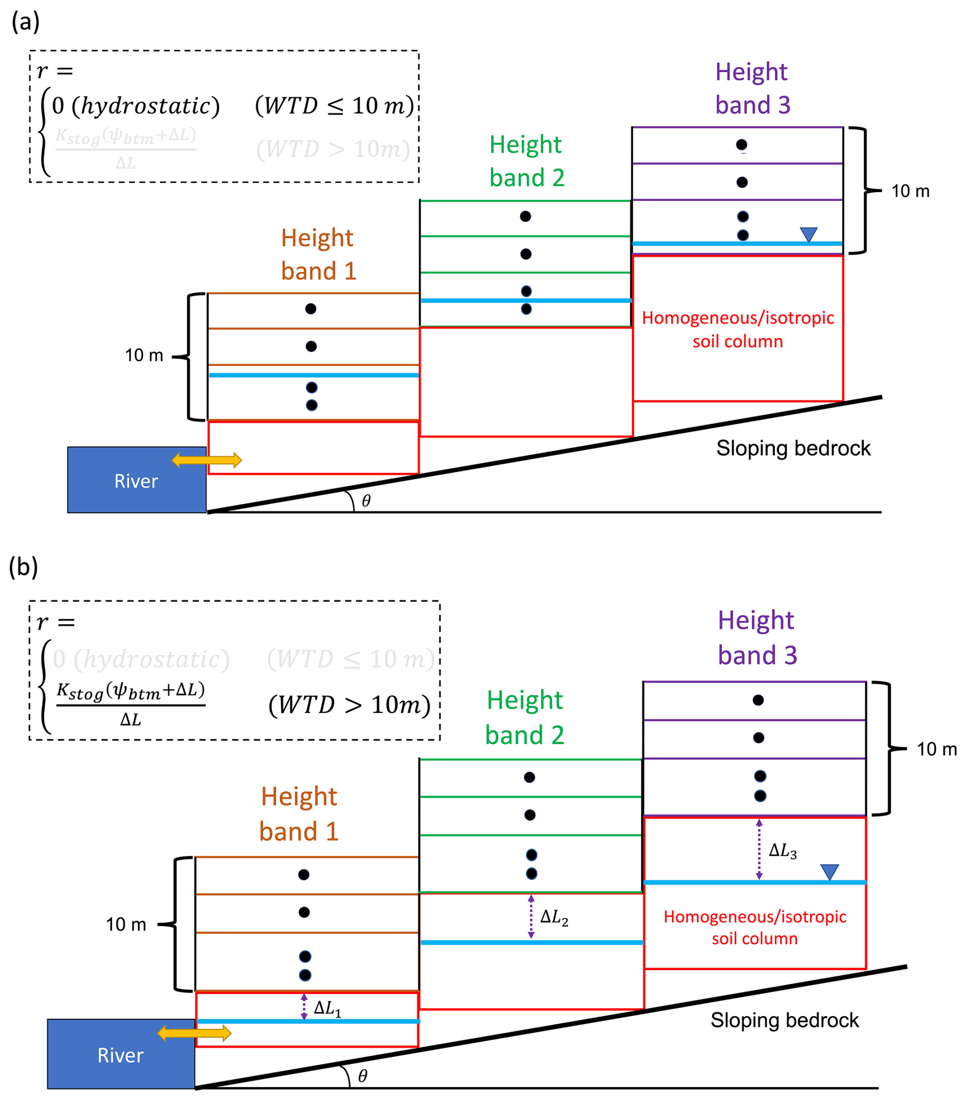
Figure 1 The LM4-SHARC's modified boundary condition (BC) at the soil base depending on the depth of the water table. (a) The equipotential line is assumed to be vertical (i.e., hydrostatic) if the depth of the water table is less than 10 m; (b) the soil base BC changes from zero flux to variable flux according to the hydraulic gradient between the bottommost soil layer and the water table. WTD denotes the water table depth. The black dots refers to the nodes located at the center of each soil layer.

2.3.2 Two-way energy transport and conservation in LM4-SHARC

LM4-SHARC accounts for the phase change of water in the groundwater domain by calculating the ice content according to the groundwater temperature (Eq. 9).

$$\begin{array}{}\text{(9)}& {\text{ws}}_{\text{gw},i}^{j+\mathrm{1}}=\left\{\begin{array}{l}{\text{ws}}_{\text{gw},i}^j-min\left({\text{ws}}_{\text{gw},i}^j\left(T_{\text{gw},i}^j-T_{\text{freeze}}\right)\frac{{\text{hc}}_{\text{gw},i}^j}{\text{hf}}\right)\\ \left({\text{ws}}_{\text{gw},i}^j>\mathrm{0},T_{\text{gw},i}^j>T_{\text{freeze}}\right)\\ {\text{ws}}_{\text{gw},i}^j+min\left({\text{wl}}_{\text{gw},i}^j\left(T_{\text{freeze}}-T_{\text{gw},i}^j\right)\frac{{\text{hc}}_{\text{gw},i}^j}{\text{hf}}\right)\\ \left({\text{wl}}_{\text{gw},i}^j>\mathrm{0},T_{\text{gw},i}^j<T_{\text{freeze}}\right),\end{array}\right.\end{array}$$

where wl_gw and ws_gw are the liquid and ice contents of the groundwater, respectively (–). T_gw is the groundwater temperature (K) and T_freeze the freezing point of 273.15 K. hf is the latent heat of fusion, a constant of $\mathrm{3.3358}\times {\mathrm{10}}^{\mathrm{5}}\mathrm{J}{\mathrm{kg}}^{-\mathrm{1}}$. hc_gw is the dynamic heat capacity of the groundwater ($\mathrm{J}{\mathrm{K}}^{-\mathrm{1}}{\mathrm{m}}^{-\mathrm{2}}$). The groundwater temperature in each HB is dynamically updated, taking into account time-dependent heat capacity (hc_gw) and heat fluxes conducted and advected from/to adjacent flow domains. Similar to the water-table-dependent boundary condition at the soil base, the heat flux boundary condition at the soil base is also affected by the groundwater condition since the water advection is zero if the water table depth is less than 10 m (Eq. 10).

$$\begin{array}{}\text{(10)}& {\mathit{\delta }}_{v_i}^j=\left\{\begin{array}{ll}\left({\mathit{\delta }}_{v_{\text{adv},i}}^j+{\mathit{\delta }}_{v_{\text{cnd},i}}^j\right)& (\text{water table depth}>\mathrm{10}\mathrm{m})\\ {\mathit{\delta }}_{v_{\text{cnd},i}}^j& (\text{water table depth}\le \mathrm{10}\mathrm{m}),\end{array}\right.\end{array}$$

where ${\mathit{\delta }}_{v_{\text{cnd},i}}^j$ is the vertical heat conduction flux, and ${\mathit{\delta }}_{v_{\text{adv},i}}^j$ is the advected heat flux between the soil column and groundwater ($\mathrm{J}{\mathrm{m}}^{-\mathrm{2}}{\mathrm{s}}^{-\mathrm{1}}$). The equations of the vertical heat conduction (${\mathit{\delta }}_{v_{\text{cnd},i}}^j$) and advection (${\mathit{\delta }}_{v_{\text{adv},i}}^j$) based on the dynamic groundwater heat capacity are addressed in Appendix A. The direction of ${\mathit{\delta }}_{v_{\text{adv},i}}^j$ is determined by the water flux (i.e., downward recharge or upward capillary) according to the hydraulic gradient. Thus, the soil columns and groundwater temperatures are simulated with the modified heat flux boundary condition (at the soil column base) from constant-thermal to variable-thermal fluxes in LM4-SHARC. The lateral heat transport in the groundwater domain (${\mathit{\delta }}_{\mathrm{l}i}^j$) is another component that determines the groundwater temperature (Eqs. 11–13).

$$\begin{array}{}\text{(11)}& {\displaystyle }& {\displaystyle }{\displaystyle }{\mathit{\delta }}_{\mathrm{l}i}^j=-q_{\mathrm{l},i}^j\text{clw}\left(T_{\text{gw},i}^j-T_{\text{freeze}}\right)(i=n_{\text{HB}})\text{(12)}& {\displaystyle }& {\displaystyle }\begin{array}{rl}{\displaystyle }{\mathit{\delta }}_{\mathrm{l}i}^j& {\displaystyle }=\\ {\displaystyle }& {\displaystyle }\text{clw}\left[q_{\mathrm{l},i+\mathrm{1}}^j\left(T_{\text{gw},i+\mathrm{1}}^j-T_{\text{freeze}}\right)-q_{\mathrm{l},i}^j\left(T_{\text{gw},i}^j-T_{\text{freeze}}\right)\right]\\ {\displaystyle }& {\displaystyle }(i=\mathrm{2},\mathrm{\dots },n_{\text{HB}}-\mathrm{1})\end{array}\text{(13)}& {\displaystyle }& {\displaystyle }\begin{array}{rl}{\displaystyle }{\mathit{\delta }}_{\mathrm{l}\mathrm{1}}^j& {\displaystyle }=\\ {\displaystyle }& {\displaystyle }\left\{\begin{array}{l}\text{clw}\left[q_{\mathrm{l},\mathrm{2}}^j\left(T_{\text{gw},\mathrm{2}}^j-T_{\text{freeze}}\right)-q_{\mathrm{l},\mathrm{1}}^j\left(T_{\text{gw},\mathrm{1}}^j-T_{\text{freeze}}\right)\right]\\ (q_{\mathrm{l}}\ge \mathrm{0})\\ \text{clw}\left[q_{\mathrm{l},\mathrm{2}}^j\left(T_{\text{gw},\mathrm{2}}^j-T_{\text{freeze}}\right)-q_{\mathrm{l},\mathrm{1}}^j\left(T_{\text{stream}}^j-T_{\text{freeze}}\right)\right]\\ (q_{\mathrm{l}}<\mathrm{0}),\end{array}\right.\end{array}\end{array}$$

where ${\mathit{\delta }}_{\mathrm{l}i}^j$ is the lateral groundwater heat flux ($\mathrm{J}{\mathrm{m}}^{-\mathrm{2}}{\mathrm{s}}^{-\mathrm{1}}$). The groundwater temperature at the ith height band at the jth time step $\left(T_{\text{gw},i}^j\right)$ is determined based on the time-dependent heat capacity and the vertical/lateral heat fluxes from/to the ith height band at the jth time step (Eq. 14).

$$\begin{array}{}\text{(14)}& T_{\text{gw},i}^{j+\mathrm{1}}=T_{\text{gw},i}^j-{\displaystyle \frac{\left[\left({\mathit{\delta }}_{v_{\text{cnd},i}}^j-{\mathit{\delta }}_{v_{\text{adv},i}}^j\right)+{\mathit{\delta }}_{\mathrm{l}i}^j\right]\mathrm{\Delta }t}{{\text{hc}}_{\text{gw},i}^j}}\end{array}$$

For the lateral heat exchange fluxes between the stream and HB₁, the stream temperature is considered if the channel loses water to the riparian zone (i.e., q_l<0). The stream temperature is estimated considering how much heat flows into the stream from the hillslopes and out of it through the catchment outlet (Eq. 15).

$$\begin{array}{}\text{(15)}& \begin{array}{rl}{\displaystyle }& {\displaystyle }{T}_{\text{stream}}^{j+\mathrm{1}}=T_{\text{stream}}^j\\ {\displaystyle }& {\displaystyle }+{\displaystyle \frac{\left[\left({\mathit{\delta }}_{\mathrm{l}\mathrm{1}}^j+{\mathit{\delta }}_{{\text{unsat}}_i}^j\right)-\text{clw}\left(T_{\text{stream}}^j-T_{\text{freeze}}\right)\frac{\mathit{\rho }{Q}^j}{A^j}\right]\mathrm{\Delta }t}{{\text{hc}}_{\text{stream}}^j}},\end{array}\end{array}$$

where ${\mathit{\delta }}_{{\text{unsat}}_i}^j$ is the heat flux advection from the unsaturated soil to the reach by interflow ($\mathrm{J}{\mathrm{m}}^{-\mathrm{2}}{\mathrm{s}}^{-\mathrm{1}}$). $Q_i^j$ is the stream discharge at the catchment outlet (m³ s⁻¹), and A^j is the flow area at the outlet at the ith height band at the jth time step. ${\text{hc}}_{\text{stream},i}^j$ is the heat capacity of the catchment outflow according to the streamflow hydrograph at the outlet ($\mathrm{J}{\mathrm{m}}^{-\mathrm{2}}{\mathrm{K}}^{-\mathrm{1}}$). Consequently, in LM4-SHARC, states and fluxes for each domain are determined by accounting for the two-way water–heat exchanges among the unsaturated soil, the hillslope aquifer, and the river.

2.4 The streamflow recession analysis for the groundwater parameterization

Brutsaert and Nieber (1977) showed that the time derivative of the recession hydrograph can be expressed as a function of the streamflow Q (Eq. 16). Since the analytical solutions to the Boussinesq equation can be recast in the form of a power law, the Boussinesq groundwater can be effectively characterized based on groundwater parameters such as K_s,f, the initial saturated groundwater thickness N_ini, and the contributing area A (Hong and Mohanty, 2023a, b; Rupp and Selker, 2006; Brutsaert and Nieber, 1977; Szilagyi et al., 1998; Tashie et al., 2021).

$$\begin{array}{}\text{(16)}& -{\displaystyle \frac{\mathrm{d}Q}{\mathrm{d}t}}=a{Q}^b,\end{array}$$

where b is a constant, and a is a function of the groundwater properties. Since the geometric similarity of unit-width Boussinesq groundwater throughout the entire catchment is assumed, the catchment outflow Q was estimated as Q=2q_lHL_reach (where L_reach is the length of the reach). This geometric similarity assumption is also reflected in the numerical estimation of the catchment outflow hydrograph (Eq. 6). Because the recession parameters a and b are readily estimated by a logarithmic regression of Q on $-\frac{\mathrm{d}Q}{\mathrm{d}t}$, streamflow observations can be used to infer the effective groundwater properties.

2.4.1 Selecting analytical models

Theoretical catchment outflow from the Boussinesq groundwater yields two hydraulic regimes: the early (i.e., high-flow) and late (i.e., low-flow) time domains. Since LM4-SHARC considers sloping groundwater, we only consider the analytical solution of the Boussinesq equation for sloping groundwater. We used the analytical solutions obtained by Brutsaert (1994), considering their applicability for a broader range of bedrock slopes (Pauritsch et al., 2015). Thus, the recession parameter a for the early time domain (a_early) is expressed in Eq. (17), with b_early set to 3.0, and the parameter a for the late time domain (a_late) is defined in Eq. (18), with b_late set to 1.0. As a result, Eqs. (17) and (18) were used to interpret the intercept (i.e., log (a)) and slope (i.e., b) of the logarithmic regression of Q on $-\frac{\mathrm{d}Q}{\mathrm{d}t}$ derived from observational streamflow data in the early time and late time domains, respectively.

$$\begin{array}{}\text{(17)}& {\displaystyle }& {\displaystyle }{a}_{\text{early}}={\displaystyle \frac{\mathrm{1.33}}{K_{\mathrm{s}}f{N}_{\text{ini}}^{\mathrm{3}}{L}^{\mathrm{2}}\cos \mathit{\theta }}},b_{\text{early}}=\mathrm{3.0}\text{(18)}& {\displaystyle }& {\displaystyle }\begin{array}{rl}{\displaystyle }{a}_{\text{late}}& {\displaystyle }={\displaystyle \frac{{\mathit{\pi }}^{\mathrm{2}}p{K}_{\mathrm{s}}{N}_{\text{ini}}{L}^{\mathrm{2}}}{f{A}^{\mathrm{2}}}}\cos \mathit{\theta }\left[\mathrm{1}+{\left({\displaystyle \frac{\frac{B}{T_{\text{ini}}}\tan \mathit{\theta }}{\mathit{\pi }p}}\right)}^{\mathrm{2}}\right],\\ {\displaystyle }& {\displaystyle }{b}_{\text{late}}=\mathrm{1.0},\end{array}\end{array}$$

where A is the subsurface drainage area (m²) that effectively contributes to the recession slope characteristics, and p is a constant set to $\mathrm{1}/\mathrm{3}$. B is the contributing groundwater's characteristic length (m) under the geometric similarity assumption, calculated as $B=A/\left(\mathrm{2}L\right)$.

2.4.2 Event-scale recession analysis

This study recognized that the recession parameters from the point cloud data (i.e., collective recession data) could be artifacts of the variability in individual recession events (REs) (Jachens et al., 2020a; Tashie et al., 2020; Karlsen et al., 2019). To fill this gap, we performed an event-scale recession analysis to account for the variability in recession slope characteristics among individual REs, which results in different estimates of groundwater properties. The onset of the REs was started 5 d after the peak to exclude the influence of overland flow (i.e., runoff) on the streamflow hydrograph. We examined the continuous decline in daily discharge observational data to decide the duration of an RE, and the end date of an RE was determined when the daily stream discharge was at its lowest.

For each RE, we performed the logarithmic regression of Q on $-\frac{\mathrm{d}Q}{\mathrm{d}t}$ in bi-logarithmic space. The time derivative of Q ($\frac{\mathrm{d}Q}{\mathrm{d}t}$) was computed based on the daily streamflow. Each RE's hydraulic regime transition point, from the early to the late time domain, was identified daily using the method suggested by Hong and Mohanty (2023a). In this method, the transition point from the early time to the late time domain is determined based on the abrupt and most noticeable change in R² values from linear regression with a fixed slope of 3.0 while incrementing the number of the data pair of $\log (-\frac{\mathrm{d}Q}{\mathrm{d}t})$–log (Q) in descending order in the bi-logarithmic space. To this end, we selectively used the daily streamflow time series of REs that lasted for more than 20 d to get enough data pairs of log (Q)–$\log (-\frac{\mathrm{d}Q}{\mathrm{d}t})$ to distinguish the hydraulic regime. For further details on the method for identifying the hydraulic regime transition in an event-scale recession analysis, see Hong and Mohanty (2023a). The process workflow of our method determining the catchment-scale hydraulic diffusivity parameters by the combined use of the analytical and numerical models is described in Fig. 2.

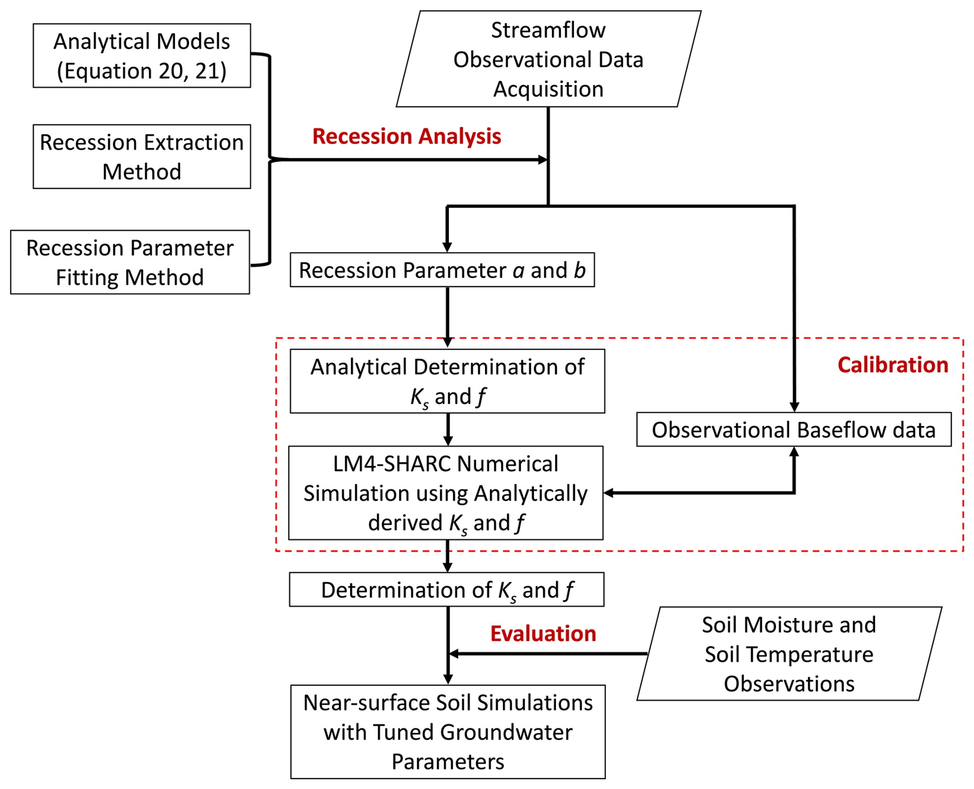
Figure 2 A workflow diagram of the method presented to calibrate and evaluate the catchment-scale groundwater diffusivity parameters based on streamflow recession analysis and the combined use of the analytical models and LM4-SHARC numerical simulations.

2.5 Experimental design for model comparison

LM4-SHARC's new parameterization for the groundwater and its interaction with the soil and river was evaluated based on a comparison of the baseflow and near-surface soil moisture/temperature outputs from the retrospective runs of LM4-SHARC and LM4-HydroBlocks, respectively. For the spinup, we used periodically cycled GSWP3 10-year forcing. The GSWP3 forcing from 1901–1910 was used repeatedly in each model cycle until a steady-state in the groundwater-related model variables was reached by replacing the initial condition for a new spinup with the final output state from the previous cycle. The groundwater-related variables include (1) soil moisture content (SMC) in the bottommost soil layer, (2) baseflow, and (3) the water table, and we considered the model to have reached a steady state if the simulated difference between the end of the nth and (n−1)th cycle for the variables used satisfied our criteria simultaneously. In this study, we set the criteria for each variable to 0 .001m³ m⁻³ (0.1 %) for the bottommost layer's SMC, 0.1 m d⁻¹ for the baseflow, and 0.001 m for the water table. We note that the soil–groundwater two-way fluxes (r in Eq. 7) were additionally considered in LM4-SHARC to evaluate a steady state, as they are a new variable in LM4-SHARC.

Using the confirmed steady state outputs as an initial condition, both model configurations were compared for the period from 1 October 2003 to 30 September 2014 (WYs 2004–2014, 11 years). In this study, the in situ precipitation and air temperature were assimilated into the GSWP3 forcing data by being directly inserted (i.e., direct insertion data assimilation). This was done to improve the accuracy of the model outputs, given the inconsistency between the GSWP3 forcing and the local meteorological conditions, which was primarily due to scale differences (i.e., 0.5°×0.5° vs. 1 km²). We considered precipitation and air temperature to be the most significant atmospheric variables determining the catchment's water and energy budgets, so the in situ precipitation and air temperature data obtained during the evaluation period replaced the corresponding variables in the GSWP3 forcing. LM4-HydroBlocks and LM4-SHARC were then operated using the identical forcing inputs. Two statistical metrics, Pearson's correlation coefficient (R²) and RMSE (root-mean-square error), were used to evaluate the temporal agreement of the modeled hydrologic outputs vs. the corresponding observations and errors, respectively.

3 Study area and observational data

3.1 Study area and the HMC parameters

The study area is the 1km² Providence Creek P301 headwater catchment in the Sierra National Forest, Nevada (Fig. 3a). The P301 headwater catchment is one of eight primary headwater catchments of the Kings River Experimental Watershed (KREW) project. The US Department of Agriculture's (USDA) Pacific Southwest Research Station initiated and operated the KREW project as part of the National Science Foundation's Southern Sierra Critical Zone Observatory (Jepsen et al., 2016; Hunsaker et al., 2012). The eight catchments are clustered into two groups, Providence and Bull, and, in this study, the P301 headwater catchment that belongs to Providence Creek was selected. We selected the P301 catchment because it contains only one first-order reach with no tributaries flowing into the reach. Since the connectivity between the catchment and reach had to be established to develop LM4-SHARC, the hydrologic configuration of the P301 catchment was considered ideal for evaluating the newly developed model.

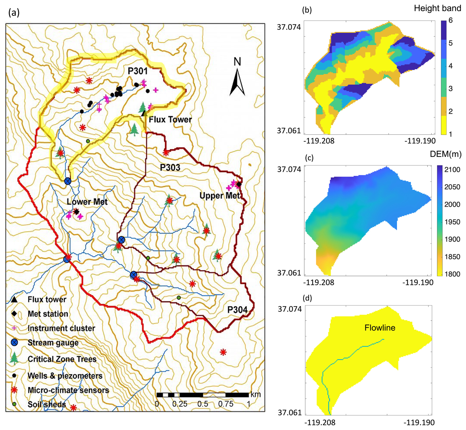
Figure 3 (a) The yellow highlighted area indicates the spatial extent of the headwater catchment P301. While the soil moisture and temperature data measured at the Lower Met station are not within the P301 catchment, the measurements from the Lower Met station were used due to the station's proximity to the catchment and the superior quantity and continuity of the observational data compared to other measurement points within the P301 catchment. (b) Using the HMC method, the P301 catchment was clustered into six different height bands (HBs). (c) The digital elevation map (DEM) of the P301 and (d) the flowline delineated by the land input dataset preprocessing. Further division of the study catchment into hillslopes is indicated in Fig. S1 in the Supplement.

Surface elevation in the P301 catchment range from 1755 to 2114 m (Hunsaker et al., 2012) on an average topographic slope of 19°. The length of the first-order reach in the P301 catchment is 1.5 km, and the average width of the reach was approximated at 10 m to define the channel geometry. The Providence P301 catchment represents a rain–snow mixed-conifer forest site with an annual mean precipitation of 1315 mm yr⁻¹. The site has a Mediterranean climate, with cool, wet winters and dry summers from approximately May through October (Safeeq and Hunsaker, 2016). During the WY 2004–2014 evaluation period, about 90 % of precipitation occurred between November and June. The mean annual air temperature was measured at 6.8 °C. Precipitation falls as a mix of rain and snow, and precipitation transitions from mostly rainfall to mostly snow at approximately 2000 m in elevation (Bales et al., 2018; Hunsaker et al., 2012).

In compiling the land input dataset for the given catchment, k was set to 1, as the study area is a single catchment. The surface elevation data from 3DEP DEM were used as the sole variable to account for the intra-catchment variability in terrain properties, and each HB's spatial extent was determined using a dh value of 20 m. p was set to 1; however, we note that the number of tiles in each HB can increase (or decrease) depending on factors such as natural mortality, land use, and fire events applied to each tile. The stream flowline was also delineated according to the 3DEP DEM using an area threshold of 100 000 m². Consequently, the P301 catchment was clustered into six HBs with a delineated area of 0.9904 km² and a stream length of 1.3 km, nearly identical to the field measurements (Fig. 3b–d).

3.2 Observations for models evaluation

3.2.1 Streamflow and baseflow

Streamflow observations measured at the outlet of the P301 catchment were used. The primary stream height measurement device is an ISCO 730 air bubbler (Teledyne Isco). Backup stage measurements were initially obtained using an AquaRod capacitance water level sensor (Advanced Measurements and Controls, Inc.) or a Telog pressure transducer (Trimble Water, Inc.). The stream height is measured at 15 min intervals and converted into the discharge rate using the standard rating curve supplied by the flume and weir manufacturers (Bales et al., 2018). The stream discharge monitoring began in September 2003 (i.e., WY 2004). The streamflow was averaged daily from WY 2004 to WY 2014 (i.e., 1 October 2003–30 September 2014, 11 years in total) and was used to evaluate the daily basis simulation outputs in this study. We derived the daily baseflow rate from the daily observational stream flow data using the baseflow separation method suggested by Szilagyi and Parlange (1998). The baseflow separation method applied assumes that the drainage from the Boussinesq groundwater maintains the stream recession flow. Thus, the baseflow separation method ensures consistency between the analytical models applied and the observational baseflow data. Szilagyi and Parlange's separation method requires the catchment area, length of channels, and the initial groundwater thickness as parameters. For consistency, the values of these parameters were determined following the parameters used in the analytical models for the recession analysis (Eqs. 17 and 18). Therefore, the catchment area (A) and channel length (L) are considered static according to the field measurement (area – 1 km²; length – 1.5 km). Applying the A value of 1 km² assumes that the entire catchment area contributes to the streamflow recession characteristics. However, if only a portion of the catchment contributes to baseflow, this assumption could create uncertainty in the baseflow estimates (Hong and Mohanty, 2023a). The initial saturated groundwater thickness N_ini, assumed to be constant at a value of 10 m across the individual REs and equivalent to the initial value of groundwater thickness applied in LM4-SHARC, could also be a source of uncertainty in the baseflow estimates. However, due to the lack of observation-based A and N_ini values, this study conducted baseflow separation under these assumptions for the two parameters.

3.2.2 Soil moisture, soil temperature, and snow depth

The soil volumetric water content (i.e., soil moisture content, SMC, and soil temperature, ST) were measured at the Lower Met using ECHO-TM sensors (METER Group). The SMC and ST were measured at 10, 30, 60, and 90 cm below the soil surface, and the measurements were used as representative values for each soil depth above and below each sensor (Bales et al., 2018). The measurements at the Lower Met station were used due to its proximity to the P301 headwater catchment (∼480 m to the outlet of the P301 catchment). The elevation difference between the Lower Met station and the nearest drainage point (i.e., reach) is about 13 m. At the station, the sensor nodes were installed at locations with different canopy coverage characteristics, such as drip edge, under canopy, and open canopy, to account for the effect of shade (i.e., radiation interception due to the canopy) on SMC and ST. Snow depth was also measured at the same Met station, and the distance to snow (or soil if no snow cover exists) was measured using an acoustic depth sensor located 3 m above the soil surface (Judd Communication LLC) (Bales et al., 2018). The sensors were installed in 2008 (i.e., WY 2009); however, due to the availability of the 10 cm depth SMC observations at the open canopy spot, the observations and simulations were compared from WY 2009 to WY 2012 (4 years). The SMC and ST observations measured at the depth nearest to the land surface (10 cm) were used to evaluate the near-surface modeled outputs from LM4-SHARC and LM4-HydroBlocks.

3.2.3 Meteorological observations

The meteorological data for model forcing were obtained concurrently from a weather station located at the Lower Met station (elevation of 1750 m). We used the SMC, ST, and snow observations. Precipitation was measured with a Belfort 5-780 shielded weighing rain gauge (Belfort Instrument) located 3 m above the soil surface. The air temperature sensor is 6 m above the soil surface (Vaisala Corporation) (Bales et al., 2018).

4 Results and discussion

4.1 Suitability of the select analytical model

We compared the analytical and numerical solutions of baseflow flux for different combinations of the groundwater diffusivity (D) and bedrock slope (θ) to test the agreement required for the application of analytically derived groundwater properties to the numerical groundwater domain. We defined the case of slow groundwater flow (SLW), with K_s of $\mathrm{2}\times {\mathrm{10}}^{-\mathrm{3}}\mathrm{mm}{\mathrm{s}}^{-\mathrm{1}}$ and f of 0.2; K_s of $\mathrm{9}\times {\mathrm{10}}^{-\mathrm{3}}\mathrm{mm}{\mathrm{s}}^{-\mathrm{1}}$ and f of 0.05 for normal groundwater flow (NRM); and K_s of $\mathrm{2}\times {\mathrm{10}}^{-\mathrm{2}}\mathrm{mm}{\mathrm{s}}^{-\mathrm{1}}$ and f of 0.02 for fast groundwater flow (FST). In each diffusivity case, the baseflow was also simulated for distinct bedrock slope conditions, such as relatively flat bedrock with a tan θ of 0.001° (MLD) and steep bedrock with a tan θ of 0.2° (STP). The hydraulic conditions, except for D and tan θ, for this gaining reach experiment are as follows: (1) river stages at jth time step at the discharge boundary follow a power function using the initial river stage $h_{\mathrm{s}}^j=h_{\mathrm{s}}^{\mathrm{0}}\times t^{-\mathrm{0.01}}$, which represents a falling limb of the hydrograph after peak discharge. (2) The initial head difference between the initial saturated groundwater thickness (N_ini) and h_s was set to the half of N_ini (i.e., $h_{\mathrm{s}}^j{\mathrm{|}}_{j=\mathrm{0}}=N_{\text{ini}}/\mathrm{2}$). Identical hydraulic conditions were applied to both analytical and numerical simulations.

The temporal agreement and the total magnitude of groundwater divergence fluxes per unit width (i.e., q_lN) were investigated during the recession duration of 15 d. As shown in Fig. 4, q_lN decreases as the hydraulic gradient between the river stage h_s and water table (at height band 1) decreases due to the discharging groundwater. For the representativeness of the time series, the R² and RMSE were estimated for the average q_lat at each time step (i.e., ${\mathit{\text{qN}}}_{\text{ave}}=\frac{q{N}_{\text{stp}}+q{N}_{\text{mld}}}{\mathrm{2}}$). The RMSE and R² were calculated at 0.00088 m² s⁻¹ and 0.98 in the SLW case, 0.0015 m² s⁻¹ and 0.97 in the NRM case, and 0.0027 m² s⁻¹ and 0.96 in the FST case. Although the gaps between the analytical and numerical qN_ave showed a bit of a drop in the agreement as the groundwater diffusivity increased, we understand that the similarly good estimation of the daily cumulative numerical qN_ave and temporal agreement (R² 0.96–0.98) could compensate for the gap and yield groundwater discharge estimates that are accurate enough to model the streamflow recession. Specifically, care needs to be taken when the analytical model is used to tune the numerical Boussinesq groundwater with extremely high D and steeper bedrock (Fig. 4c). Except for such hydraulically extreme cases that are unrealistic in real catchments (i.e., $D>\mathrm{1.0}\mathrm{mm}{\mathrm{s}}^{-\mathrm{1}}$), the numerical simulation of the Boussinesq groundwater's discharge with analytically tuned parameters can be justifiable.

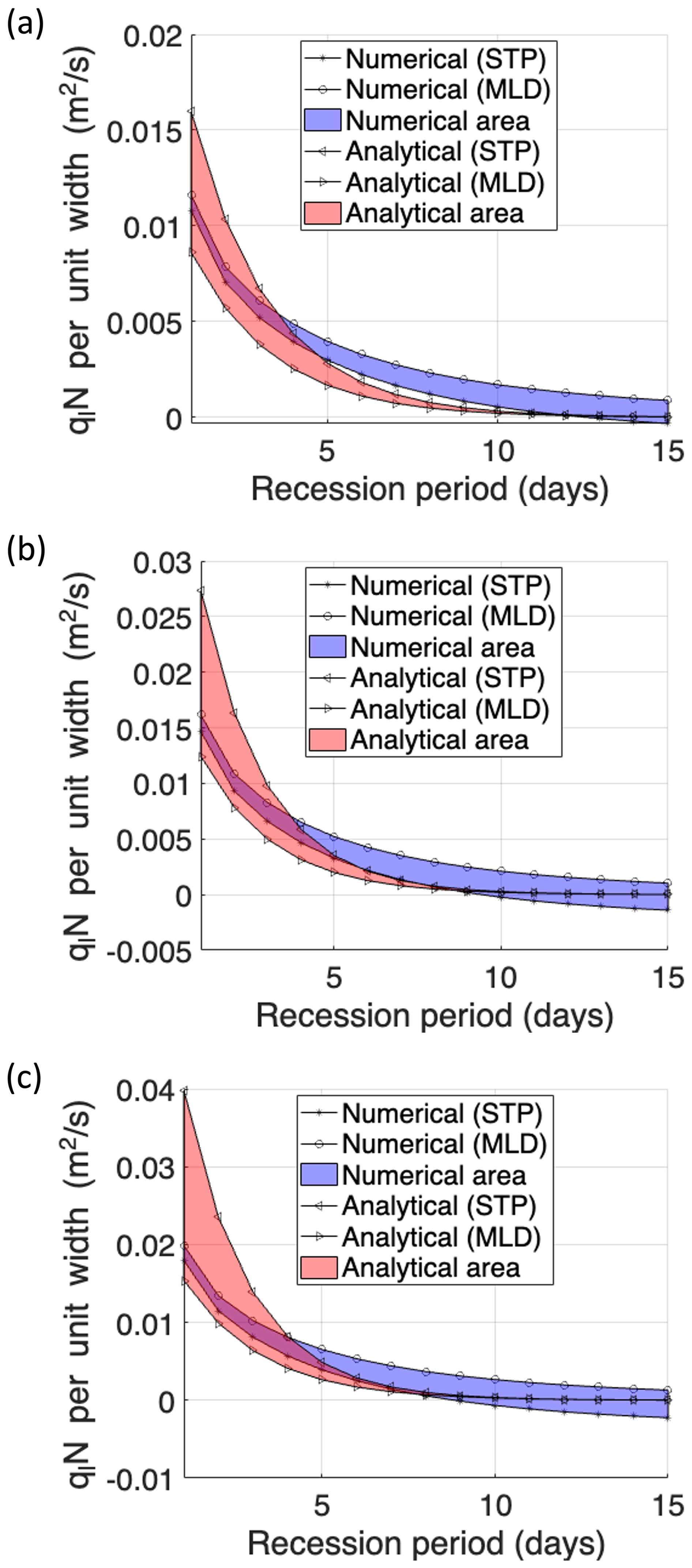
Figure 4 Comparison between the baseflow flux solutions derived from the analytical and numerical models selected. (a) The SLW case with K_s of $\mathrm{2.0}\times {\mathrm{10}}^{-\mathrm{3}}\mathrm{mm}{\mathrm{s}}^{-\mathrm{1}}$ and f of 0.20. (b) The NRM case with K_s of $\mathrm{9.0}\times {\mathrm{10}}^{-\mathrm{3}}\mathrm{mm}{\mathrm{s}}^{-\mathrm{1}}$ and f of 0.05. (c) The FST case with K_s of $\mathrm{2.0}\times {\mathrm{10}}^{-\mathrm{2}}\mathrm{mm}{\mathrm{s}}^{-\mathrm{1}}$ and f of 0.02. The numerical and analytical areas refer to the uncertainty bands of numerical and analytical solutions due to slope variations.

4.2 Event-scale recession analysis and calibration

4.2.1 Quantifying the uncertainty in hydraulic diffusivity estimates

We performed the event-scale recession analysis to estimate the effective groundwater properties of the study catchment. Following the extraction criteria (Sect. 2.4.2), 18 individual REs were extracted from the 13-year series of streamflow observations, and the recession parameters a and b were estimated for each hydraulic regime (Table 1). Figure 5a presents an example showing how an individual RE was analyzed with the selected analytical models for its early and late time domains using daily streamflow data from the P301 catchment. Once the recession parameters a and b were estimated for each RE, the range of bedrock slope θ should be adequately constrained in order to determine the hydraulic diffusivity parameters K_s and f. The characteristic length B is calculated by assuming the geometric similarity between both sides of the hillslope in the catchment; thus, $B=A/\left(\mathrm{2}L\right)$. The following criteria were applied to define the upper and lower bounds of θ: (1) the effective porosity f should range from 0.1 % to 20.0 % (Brutsaert and Lopez, 1998; Tashie et al., 2021; Troch et al., 1993; Hong and Mohanty, 2023b, a; Heath, 2004), and (2) the catchment-scale effective groundwater lateral hydraulic conductivity K_s cannot exceed 1.0 mm s⁻¹ (Fan and Miguez-Macho, 2011; Gómez-Hernández and Gorelick, 1989; Tashie et al., 2021).

Table 1 Recession period, recession characteristics, and parameters a and b for each recession event under different diffusivity conditions. The variability in the parameter a indicates the variability in the distinct diffusivity of groundwater across individual recession events.

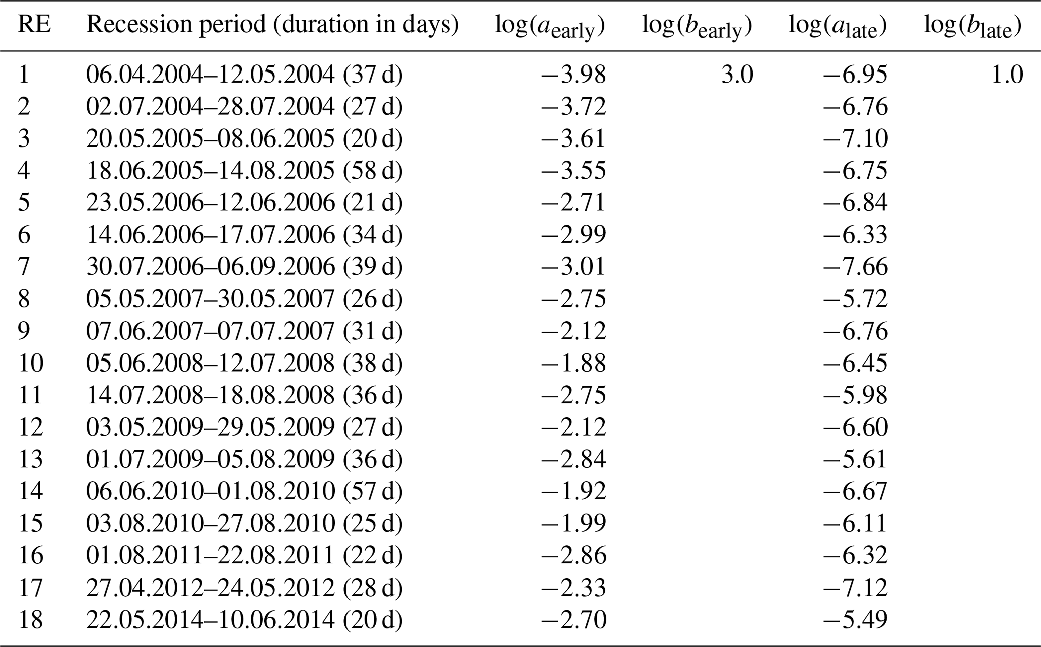
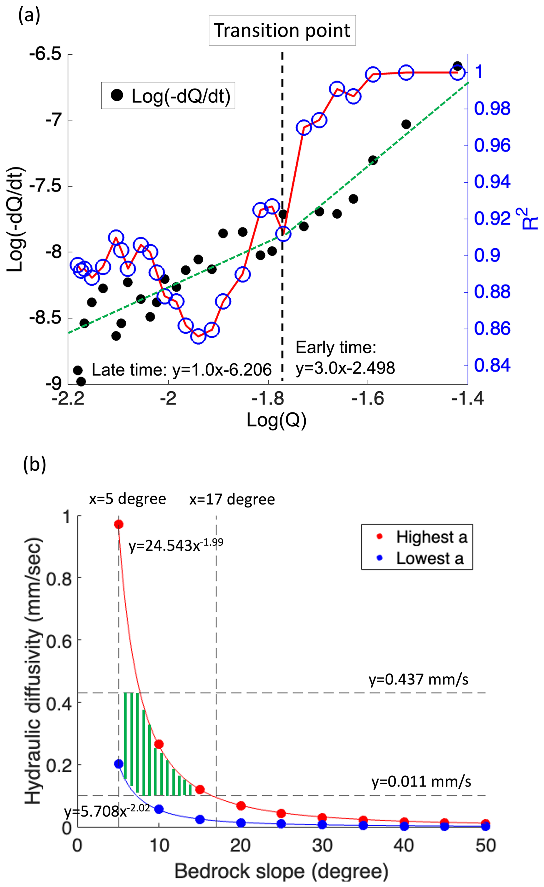
Figure 5 (a) An example showing how the transition point of a hydraulic regime (from the early to the late time domain) is determined from an individual recession event. Understanding the combined recession parameters a_early and a_late enables us to infer the groundwater properties such as hydraulic diffusivity D. (b) The uncertainty in the groundwater properties D and θ was constrained by the power function relationship between them, which results from the variability in the recession parameter a across individual recession events.

The variability in recession characteristics was quantified by the recession parameter a (since b is fixed) in the early and late time domains (i.e., a_early and a_late) (Fig. 5b). Essentially, this parameter provides insights into the variability in the groundwater's effective properties dependent on the memory effects of the catchment (e.g., groundwater storage). The 98 % confidence intervals for a_early and a_late were estimated to be [$-\mathrm{3.10},-\mathrm{2.43}$] and [$-\mathrm{6.81},-\mathrm{6.20}$], respectively, from the analysis of 18 REs. Following the above criteria, the value distributions of K_s, f, and θ corresponding to the ranges of a_early and a_late were estimated. The uncertainty in K_s, f, and θ was then quantified by determining the intersection range between K_s, f, and θ values derived from the lowest a (i.e., $\log (-\frac{\mathrm{d}Q}{\mathrm{d}t})=-\mathrm{3.10}\log \left(\mathrm{d}Q\right)-\mathrm{6.81})$ and the highest a (i.e., $\log (-\frac{\mathrm{d}Q}{\mathrm{d}t})=-\mathrm{2.43}\log \left(\mathrm{d}Q\right)-\mathrm{6.20})$. The upper and lower bounds of K_s were thus estimated as [0.0026, 0.0138 mm s⁻¹]. For f, the bounds were identified as [0.033, 0.190], and for θ they were [5.0, 17.0°]. Also, for each set of data pairs of $\log (-\frac{\mathrm{d}Q}{\mathrm{d}t})-\log \left(\mathrm{d}Q\right)$ with the lowest and highest a, the relationship between hydraulic diffusivity (per unit of wetted perimeter) D and the bedrock slope θ follows a power function. Consequently, we considered the (θ,D) space in which solutions of D and θ (potentially representing the catchment average behavior) could exist to be further constrained by the range of parameters specified, K_s, f, and θ, between the power functions (Fig. 5b).

4.2.2 Calibrating groundwater properties based on baseflow flux accuracy

While the groundwater properties vary across the REs due to the catchment's memory effect, the groundwater properties that represent the long-term average behavior of the groundwater need to be tuned in the LM4-SHARC groundwater domain. Based on the value range of θ and D that was identified, we tried to determine a single pair of (θ,D) that shows the optimal accuracy by comparing the modeled and observed baseflow data. The modeled baseflow fluxes were estimated by summing the liquid fluxes from saturated soil to the stream, and baseflow observations during this study's evaluation period (from 1 October 2003 to 30 September 2014, WYs 2004–2014) were used for calibration. We considered a (θ,D) that best represents the temporal dynamics and magnitudes of baseflow observations to be the calibrated (θ,D) for the study catchment.

We identified the fact that a specific parameter pair (θ,D) can be specified in the uncertainty space. Figure 6 shows that (1) the temporal agreement between the modeled and observed baseflow was generally related to the magnitude predictions and (2) the most significant improvements to R² and RMSE (from LM4-HydroBlocks to LM4-SHARC) were identified at the same time at a specific pair of (θ,D). We found the most pronounced improvements to the baseflow predictions in LM4-SHARC compared to LM4-HydroBlocks, with an R² improvement of 0.155 and an RMSE reduction of 0.220 mm d⁻¹ at θ=5.0° and $D=\mathrm{4.6}\times {\mathrm{10}}^{-\mathrm{2}}\mathrm{mm}{\mathrm{s}}^{-\mathrm{1}}$. The R² and RMSE of the LM4-SHARC-derived baseflow estimates vs. the observations (over the 11 years) were estimated at 0.402 and 0.556 mm d⁻¹, while those of the LM4-derived baseflow estimates were estimated at 0.247 and 0.776 mm d⁻¹, respectively. With the calibrated groundwater properties, we confirmed that the recession behaviors of the P301 catchment streamflow hydrograph over the 11-year evaluation period were generally better captured in the LM4-SHARC baseflow estimates compared to those of LM4-HydroBlocks (Fig. 7).

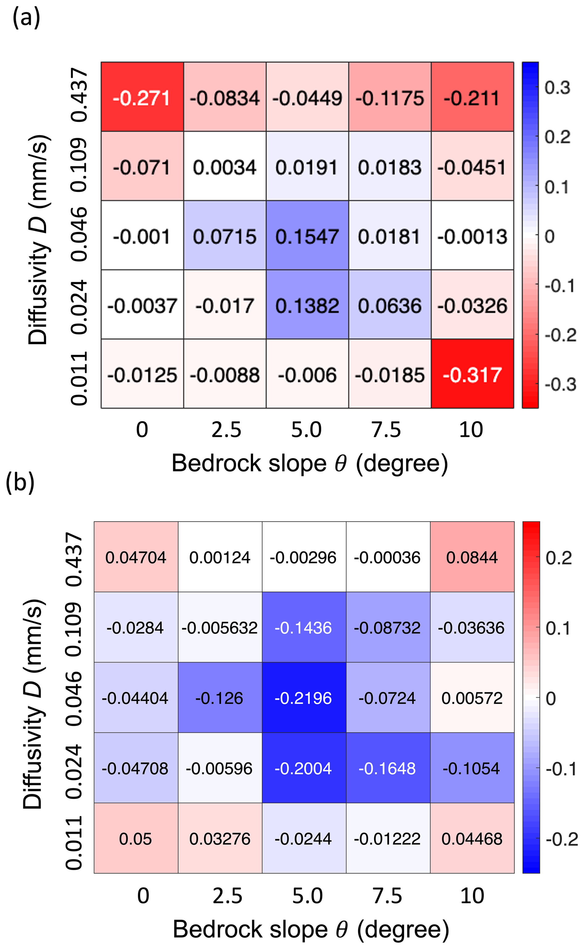
Figure 6 A pair of groundwater parameters (θ,D) was specified to calibrate the catchment groundwater. (a) The R² difference (improvement) between LM4-SHARC and LM4-HydroBlocks ($R_{\text{LM4-SHARC}}^{\mathrm{2}}-R_{\text{LM4-HydroBlocks}}^{\mathrm{2}}$). Here, R² denotes the coefficient of determination between the modeled baseflow and observations for the 11-year evaluation period. (b) For the same period, the RMSE difference (reduction) between LM4-SHARC and LM4-HydroBlocks (RMSE_LM4-SHARC−RMSE_{LM4-HydroBlocks}) was evaluated.

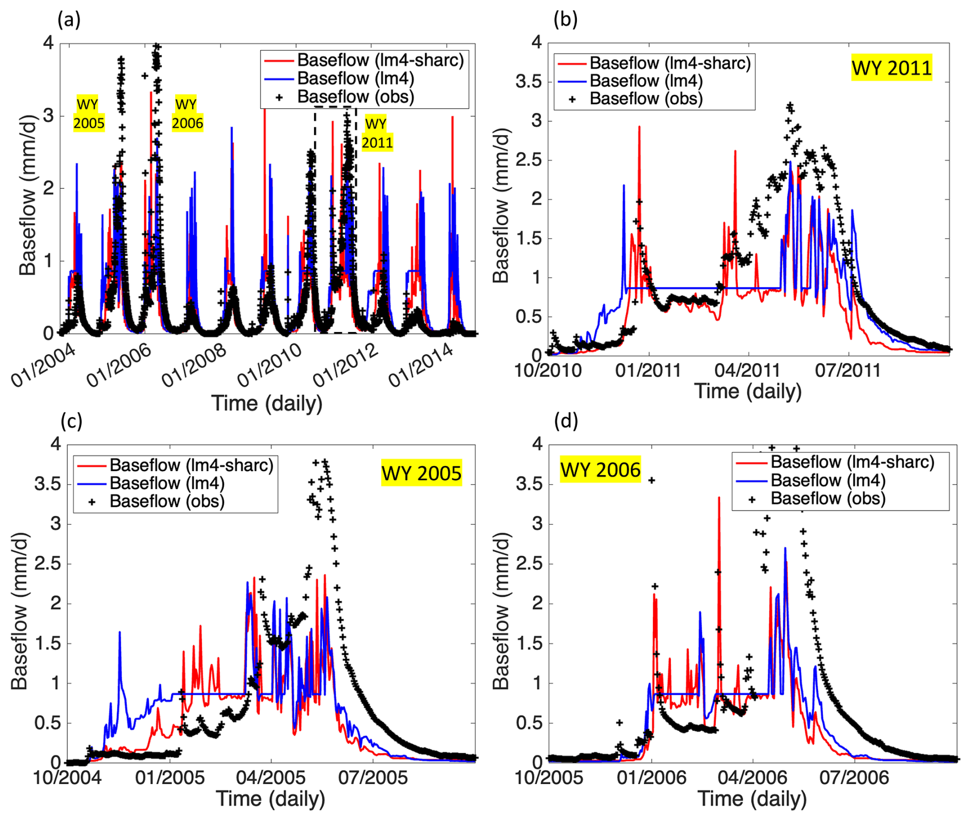
Figure 7 Comparative time series of baseflow estimates from LM4-SHARC (red), LM4-HydroBlocks (LM4 in the legend, blue), and the corresponding observations. (a) Daily time series of the baseflow data over the evaluation period of 11 years. (b) Time series in water year (WY) 2011, (c) time series in water year (WY) 2005, and (d) time series in water year (WY) 2006. The streamflow recession behavior was generally better represented in LM4-SHARC compared to LM4-HydroBlocks.

4.3 The effect of groundwater on near-surface water and energy balances

4.3.1 Near-surface soil moisture and temperature predictions

Using the calibrated groundwater diffusivity properties, we assessed the effects of groundwater-induced soil processes on the near-surface water and energy budgets. We applied θ=5.0° and $D=\mathrm{4.6}\times {\mathrm{10}}^{-\mathrm{2}}\mathrm{mm}{\mathrm{s}}^{-\mathrm{1}}$ to tune the Boussinesq groundwater domain (in LM4-SHARC) and compared the soil moisture and temperature estimates at 10 cm in depth from both configurations. The evaluation of near-surface soil moisture and temperature predictions was performed for 4 years, from WY 2009 to WY 2012. Figure 8a–d show the comparative time series of 10 cm depth soil moisture, soil temperature, and snow mass among LM4-HydroBlocks, LM4-SHARC, and in situ observations in each WY. From all 4 years of the evaluation period, we identified the fact that soil bottom drainage (SBD) facilitation due to the modified boundary condition from zero-flux to variable-flux BC at the base of the soil columns (Fig. 1a) significantly affected the soil moisture content (SMC) at 10 cm in depth. The time series of 10 cm SMC from LM4-SHARC showed significantly reduced SMC compared to that of LM4-HydroBlocks. The entire soil column reached full saturation too quickly in LM4-HydroBlocks, and the downward liquid transport facilitated due to drier lower layers of soil in LM4-SHARC was found to be effective in correcting the soil's wet biases. As a result, the temporal variability and total storage of the observed SMC was better captured in LM4-SHARC. The average of the four R² values from the yearly time series comparison (i.e., 2009–2012) improved from 0.831 (LM4-HydroBlocks) to 0.849 (LM4-SHARC), while noticeably reducing the average RMSE from 0.0722 m³ m⁻³ (LM4-HydroBlocks) to 0.0425m³ m⁻³ (Fig. 9a and b).

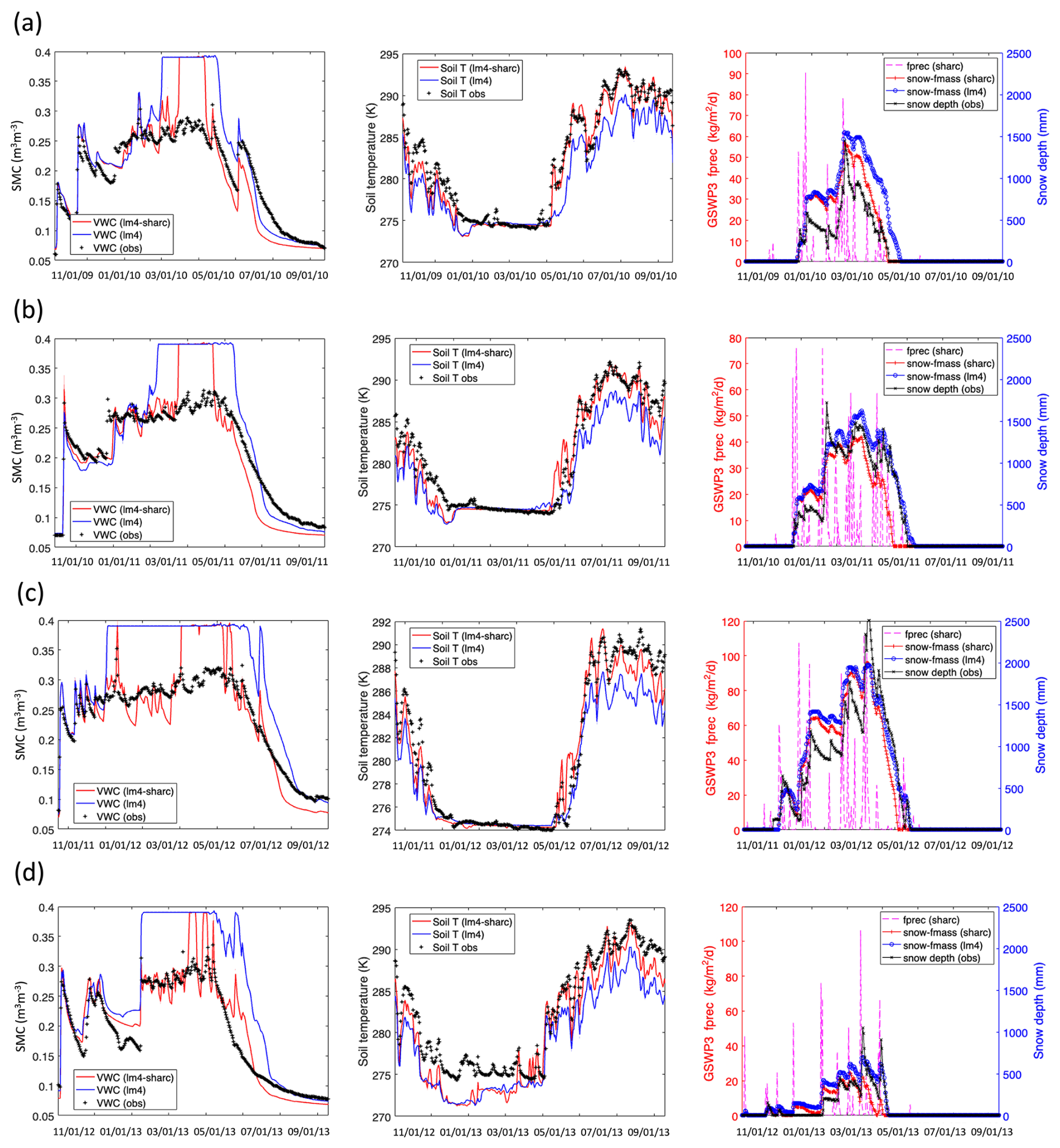
Figure 8 Comparative yearly time series of soil moisture, temperature, and snow mass for the evaluation periods in (a) WY 2009, (b) WY 2010, (c) WY 2011, and (d) WY 2012. For all years, higher soil temperature at 10 cm in depth due to drier soil was generally identified. GSWP3 fprec (y-axis label in the third column) stands for frozen precipitation, denoting the snowfall rate in units of $\mathrm{kg}{\mathrm{m}}^{-\mathrm{2}}{\mathrm{d}}^{-\mathrm{1}}$.

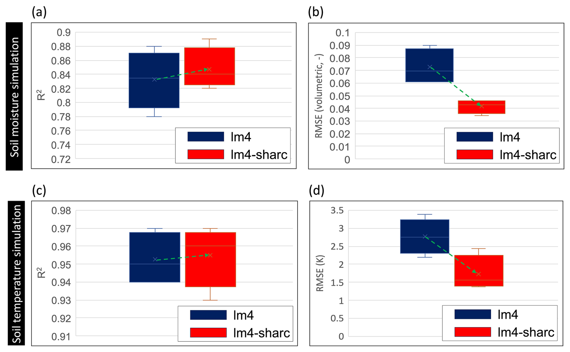
Figure 9 (a, b) The average of the four R² from the yearly time series comparison of 10 cm depth soil moisture (i.e., 2009–2012) improved from 0.831 (LM4-HydroBlocks) to 0.849 (LM4-SHARC), while significantly reducing the average RMSE from 0.0722 m³ m⁻³ (LM4-HydroBlocks) to 0.0425 m³ m⁻³. (c, d) R² from the yearly time series comparison between the modeled and observed soil temperature at 10 cm in depth increased from 0.952 to 0.957, and the RMSE significantly decreased, from 2.77 to 1.67 K. LM4 denotes LM4-HydroBlocks.

We also found that the enhanced representation of SMC resulted in better capture of near-surface soil temperature dynamics. The decreased SMC reduces the evapotranspiration rate, especially during daytime, leading to increased sensible heat in the soil's energy balance. Also, the reduced soil heat capacity due to decreased SMC (i.e., liquid water) increased the soil temperature under the given net radiation. Consequently, we identified the fact that soil temperature predictions at the 10 cm depth showed significant improvements in LM4-SHARC, primarily during warmer seasons, and showed better agreement with the observations. The soil temperature estimates from both model configurations showed similar values when the surface was covered by snow (i.e., snow depth>0). In this case, the soil is insulated by snow and thus variations in soil water predicted by the two model configurations do not lead to appreciable differences in soil temperature. From the improved skill in predicting near-surface soil temperature in LM4-SHARC, we conclude that the soil columns with applied zero-flux BC at 10 m in depth could hold too much soil water due to the shallow water table imposed. This overestimation in soil water content could lead to an inaccurate description of the land energy balance (e.g., overestimated ET/less sensible heat) and thus to biases in soil temperature. We note that the average of the four R² values from the yearly time series comparison between the modeled and observed soil temperature increased from 0.952 to 0.957, and the RMSE significantly decreased, from 2.77 to 1.67 K (Fig. 9c and d).

The simulated snow depth from both LM4-HydroBlocks and LM4-SHARC generally showed reasonable agreement with the measured snow depth in the catchment. We note that the meltout timing of snow involves the mutual influence of soil temperature. Specifically, we noticed that the timing of snow meltout is affected by soil temperature, as the warmer ground expedites the melting. The meltout timing of snow in the 4 evaluation years was represented sooner in LM4-SHARC than LM4-HydroBlocks due to increased soil temperature (Fig. 8). Also, as the snow melted out, the soil temperature quickly increased, as the soil was no longer insulated by snow, leading to a higher correlation with surface air temperature.

4.3.2 Sensitivity of soil water storage to stream–groundwater diffusivity

After examining the enhancement in the catchment-scale water and energy balance, we further explored to what extent groundwater properties affect soil processes in LM4-SHARC, focusing on soil water storage (SWS). We investigated the sensitivity of SWS to the groundwater properties θ and D by estimating differences in SWS per unit area (i.e., ΔSWS (kg m⁻²)) between LM4-SHARC and LM4-HydroBlocks. ΔSWS was calculated by subtracting the total SWS per unit area of the soil columns (in the catchment), which was derived from LM4-HydroBlocks, from that of LM4-SHARC at the end of the simulation. To this end, we need to verify that the model reaches a steady state for the given groundwater properties. The variability in SWS (ΔSWS) is evaluated only after the steady state has been reached. Figure 10a–d show that the simulations of the four variables reduce their deviations (from the previous cycle) as the cycles progress and that the model was considered to be steady state based on the agreement of variables from the nth and (n−1)th cycles. We also identified the fact that the groundwater properties influenced the time to reach a steady state (i.e., spinup time), as the variations in groundwater diffusivity affect the flux velocity. More detail can be found in Fig. S2 in the Supplement.

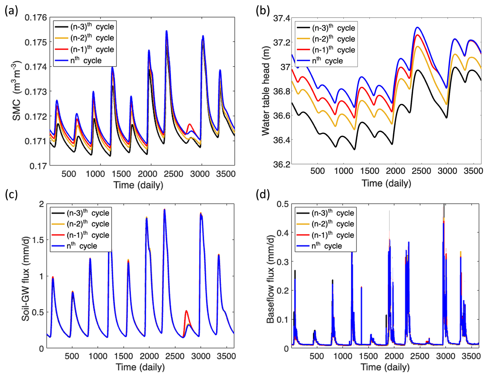
Figure 10 (a) The volumetric soil moisture content at the bottommost soil layer. (b) The groundwater table. (c) The groundwater recharge fluxes (positive). (d) The baseflow fluxes reduce their deviations (compared to the previous cycle) as the cycles progress. They are considered steady state based on the differences between the nth and (n−1)th cycle.

ΔSWS due to groundwater discharge was investigated based on the steady state of the model. The working hypothesis here is that the lateral groundwater discharge could facilitate the SBD by inducing downward hydraulic gradients from the subsurface soil and water table. Figure 11a shows the variability and magnitude of the entire catchment's annual mean of ΔSWS (over 10 years) according to θ and D (y-axis values denote the average ΔSWS per soil column). It is noticeable that the annual mean of ΔSWS gradually increased negatively (i.e., less SWS in LM4-SHARC) with increasing D until the water table dynamics did not significantly affect hydraulic gradients between subsurface soil and the water table (i.e., lack of groundwater storage). This happened when the downward groundwater recharge fluxes were continuously less than q_l in the groundwater domain. Also, the catchment's total ΔSWS was found to be lower if the slope is steep. While the steeper bedrock showed a greater q_l with the increased gravitationally driven discharge fluxes, ΔSWS values were more noticeably affected by the lowered water table due to relatively flatter bedrock in the groundwater domain. In the case of this catchment, it was also observed that for D values greater than 0.1 mm s⁻¹, the lack of groundwater storage occurred irrespective of the bedrock slope.

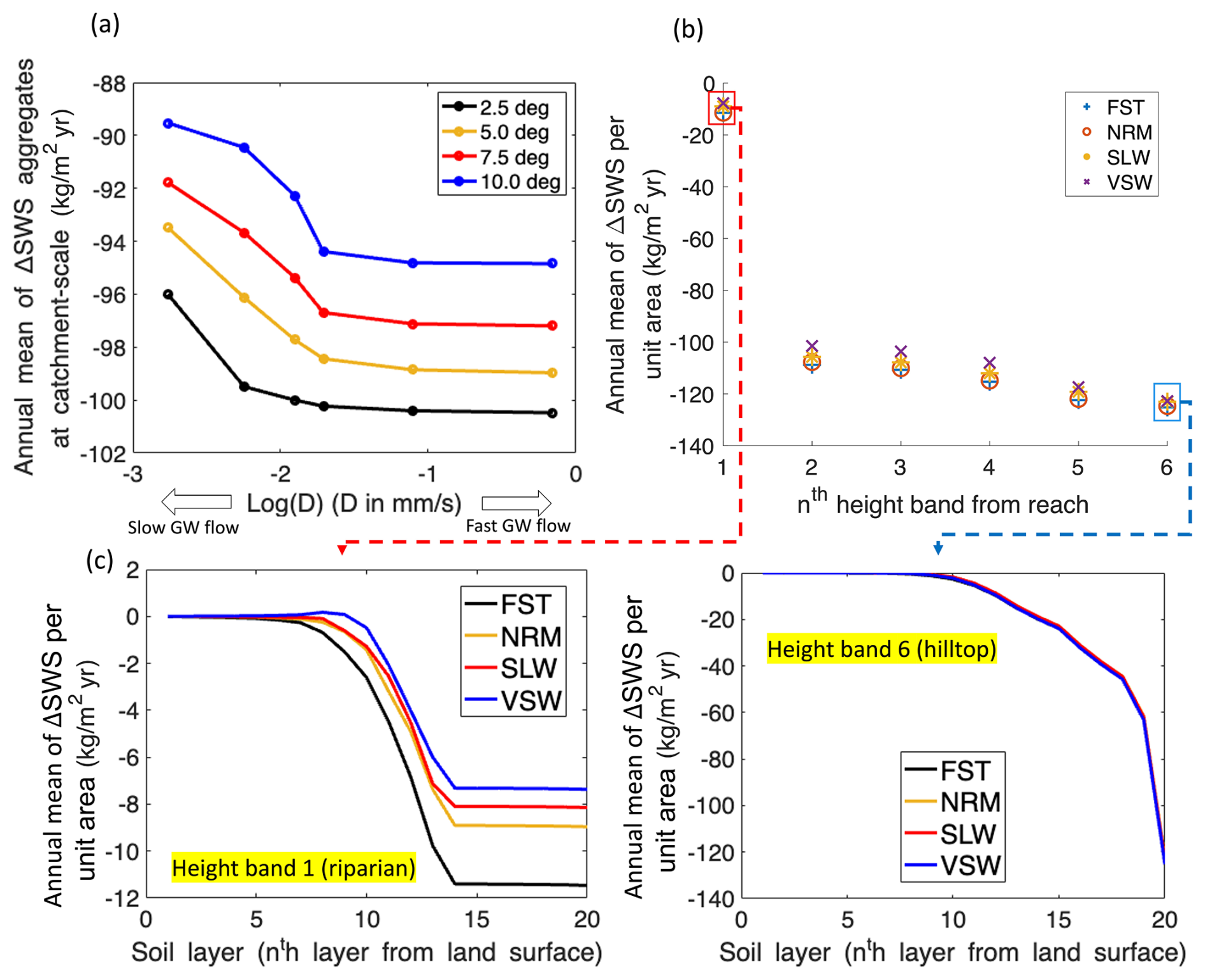
Figure 11 (a) Sensitivity of soil water storage (SWS) to the diffusivity D and bedrock slope θ. (b) The soil drainage (i.e., downward recharge) due to the groundwater lateral discharge was more noticeable as the height band was farther from the reach. (c, d) More-significant effects of groundwater flow conditions on the SWS in the riparian zone compared to those in the hilltop area.

Moreover, SBD facilitation due to the groundwater lateral discharge was more noticeable, as the height band was farther from the reach. The annual mean of ΔSWS per unit area gradually decreased from HB₆ ($\sim \mathrm{120}\mathrm{kg}{\mathrm{m}}^{-\mathrm{2}}{\mathrm{yr}}^{-\mathrm{1}}$) to HB₁ ($\sim \mathrm{10}\mathrm{kg}{\mathrm{m}}^{-\mathrm{2}}{\mathrm{yr}}^{-\mathrm{1}}$), with a sharp decrease at HB₁ (Fig. 11b). It was also noticeable that the distinct D made less difference among the values of ΔSWS per unit area, as the height band was farther from the reach. Figure 11c and d illustrate that the effects of groundwater flow conditions on the SWS variability could be more significant in the riparian/river valley compared to the hilltop area. This also implies that the groundwater effects on the water content in the partially saturated soil depend on the depth of the water table, leading to higher sensitivity of SMC to groundwater diffusivity if the water table is shallow than if it is deep. While the HB₆ annual ΔSWS per unit area (m²) values were the greatest among HB₁ to HB₆, ranging from 121.45 $\mathrm{kg}{\mathrm{m}}^{-\mathrm{2}}{\mathrm{yr}}^{-\mathrm{1}}$ (VSW, very slow) to 121.89 mm (FST), the ΔSWS difference (between VSW and FST) of 0.44 $\mathrm{kg}{\mathrm{m}}^{-\mathrm{2}}{\mathrm{yr}}^{-\mathrm{1}}$ was minor compared to the result from HB₁. From HB₁, the ΔSWS values were found to range from 7.75 $\mathrm{kg}{\mathrm{m}}^{-\mathrm{2}}{\mathrm{yr}}^{-\mathrm{1}}$ (VSW) to 11.70 $\mathrm{kg}{\mathrm{m}}^{-\mathrm{2}}{\mathrm{yr}}^{-\mathrm{1}}$ (FST), yielding a difference of 3.94 $\mathrm{kg}{\mathrm{m}}^{-\mathrm{2}}{\mathrm{yr}}^{-\mathrm{1}}$ due to the groundwater diffusivity.

4.4 Distinct vegetation characteristics in the catchment due to hydrologic contrast

The water convergence due to the groundwater lateral flow induces the hydrologic contrast at the catchment scale, leading to distinct vegetation characteristics depending on the distance from the river (Fan et al., 2019). Here, we used the modeled leaf-area index (LAI) to infer distinct vegetation characteristics (i.e., plant density) in the study catchment. The LAI was simulated from 1901 to 2014 (114 years) in both model configurations without spinup using the GSWP3 forcing with assimilated in situ precipitation/air temperature data (i.e., GSWP3 (January 1901–September 2003) and in situ data (October 2003–September 2014)). Comparison of the LAI time series between LM4-SHARC and LM4-HydroBlocks revealed that the differences in the LAI in the hilltop area (i.e., HB₆) were more dramatic than those in the riparian zone (i.e., HB₁) as the vegetation evolved (Fig. 12a and b). With a closer look at the LAI time series for the recent 4 water years (i.e., WYs 2009–2012, as studied in Sect. 5.3.1) in the riparian zone and on the hilltop, we found that the LAI contrast was, moreover, more significant during the warmer season in the hilltop area, while the overall trend in the LM4-SHARC-derived LAI evolved comparably to that of the LM4-derived LAI in the riparian zone (Fig. 12c and d). The hydrologic convergence in the riparian zone explains the comparable LAI dynamics in the riparian zone, as the subsoil domain readily saturated by the converging water impedes SBD, leading to higher water retention in the partially saturated soil. Different soil moisture availability (between HB₁ and HB₆) resulting from the contrasting SBD dynamics is thus emphasized by the density of plants, especially during the warm(er) season when the plants yield higher transpiration rates. The varied transpiration rates in LM4-SHARC also consistently explain the LAI contrast due to different soil moisture conditions. We found that the transpiration rate on the hilltop was reduced by 29.5 % in LM4-SHARC, while the rate was reduced by 10.3 % in the riparian zone in LM4-SHARC (Fig. 12e and f). Overall, we found that the variations in SWS, transpiration, and LAI simulations are consistent in that the groundwater convergence to the river valley intensified the catchment's contrasting hydrologic states.

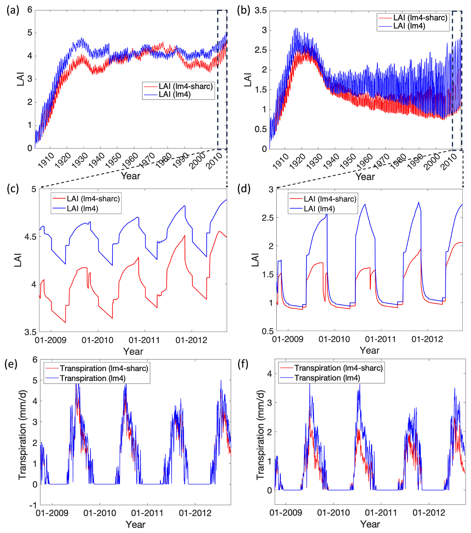
Figure 12 Temporal evolution of LAI from 1901 to 2014 (114 years) using GSWP3 forcing at (a) the riparian zone (HB1) and (b) the hilltop (HB6). The differences in the LAI (between LM4-SHARC and LM4-HydroBlocks) in the hilltop area were more dramatic than those in the riparian zone. (c, d) The LAI time series for the recent 4 WYs (i.e., WY 2009–2012) and (e, f) the time series of the plant transpiration rate (mm d⁻¹) for the same period. LM4 denotes LM4-HydroBlocks. The effects of varying transpiration dynamics in LM4-SHARC on evapotranspiration estimates are discussed in Fig. S3 in the Supplement.

4.5 Applicability of LM4-SHARC in an ESM

4.5.1 Testing LM4-SHARC in various climatic and orographic zones

To support the implementation of LM4-SHARC in the GFDL ESM, we need to investigate the performance of LM4-SHARC in various climatic and orographic zones. For this purpose, three additional headwater catchments were selected based on their precipitation and topographic slope characteristics (Fig. 13a): the Musselshell (MT), Maine (ME), and Clearwater (WA) headwater catchments. The precipitation and slope characteristics of these sites vary from those of the Clearwater catchment (the wettest, 3136 mm yr⁻¹, and steepest, 0.547 m m⁻¹, catchment) to those of the Musselshell catchment (the driest, 397 mm yr⁻¹, and flattest, 0.094 m m⁻¹). In this experiment, the groundwater properties in the additional catchments were assumed to be identical to those of the P301 headwater catchment, so diffusivity D was set to 0.046 mm s⁻¹ and the slope of the groundwater bedrock θ was assumed to be 5° in all three headwater catchments. The steady state of the groundwater and any adjacent flow domains was also ensured, and the evaluation was performed using the 10-year model outputs.

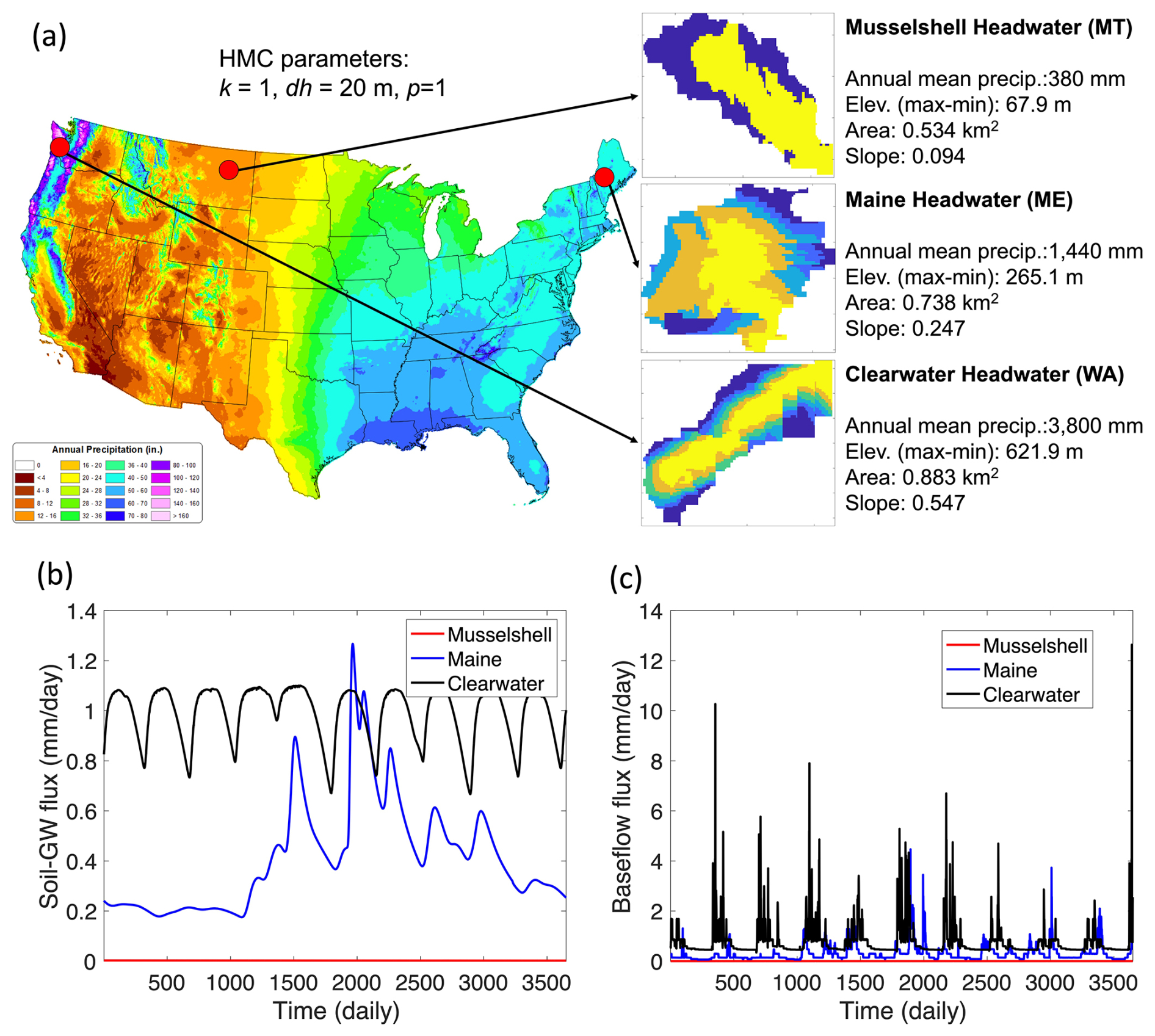
Figure 13 (a) The three additional sites are marked (red dots) on the PRISM 30-year normal precipitation map (2022, PRISM Group, Oregon State University). The sites include the Musselshell headwater (MT), Maine headwater (ME), and Clearwater headwater (WA) catchments. (b) LM4-SHARC's daily soil–groundwater exchange fluxes (mm d⁻¹) over 10 years from the three catchments and (c) the simulated daily baseflow fluxes (mm d⁻¹) for the corresponding period and sites.

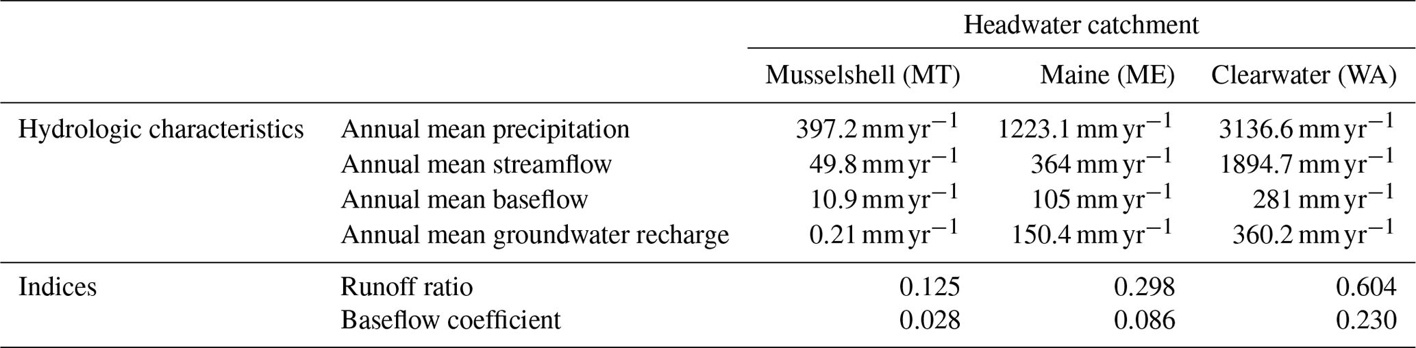
We tried to identify whether the model is robust under diverse conditions by examining the consistency between hydrologic characteristics and indices. The hydrologic indices include (1) the runoff ratio (i.e., the ratio of streamflow to precipitation) and (2) the baseflow coefficient (i.e., the ratio of baseflow to precipitation). The annual mean baseflow/streamflow of each catchment was estimated at 10.9$/$49.8 mm yr⁻¹, 105$/$364.0 mm yr⁻¹, and 281$/$1897.4 mm yr⁻¹ from the Musselshell, Maine, and Clearwater catchments, respectively. Using the respective annual mean precipitation of each catchment (i.e., Musselshell – 397.2 mm yr⁻¹; Maine – 1223.1 mm yr⁻¹; and Clearwater – 3136.6 mm yr⁻¹), each catchment's baseflow coefficient/runoff ratio was estimated at $\mathrm{0.028}/\mathrm{0.125}$, $\mathrm{0.086}/\mathrm{0.298}$, and $\mathrm{0.230}/\mathrm{0.604}$. The established positive correlation between the baseflow coefficient and runoff ratio is consistent with what has been reported in previous studies (Cheng et al., 2021; Ouyang et al., 2018) (Table 2). We also found that the value gradients of baseflow/recharge estimates correspond to what is expected from the slope/precipitation gradients. For example, the highest yield of baseflow from the Clearwater catchment (i.e., 0.77 mm d⁻¹) can be explained by its high precipitation and steep slope, which contribute to higher drought flow (i.e., baseflow during dry seasons) and peaks. Also, the partially saturated soil found in most parts of the Musselshell catchment explains the minimal baseflow amounts due to the lack of groundwater storage from the limited groundwater recharge (Fig. 13b and c).

Table 2 The hydrologic characteristics and indices of the three additional headwater catchments from the simulated outputs with the GSWP3 forcing from 1901 to 1910. The annual mean values of each catchment are estimated from the 10-year cycle based on the confirmed steady state.

4.5.2 Inferring groundwater properties for global-scale SHARC simulations

Since the parameterization scheme SHARC presented in this paper relies on the observationally derived recession characteristics of streamflow, a method must be developed to quantify the recession variability (using the parameter a) of catchments with no streamflow information. This necessity is particularly emphasized, as the SHARC scheme will ultimately be used for global simulations. While not providing specific research findings, this section aims to discuss several possible approaches based on existing studies. Essentially, we expect that existing global-scale datasets of soil, topography, climatology, and remotely sensed hydrologic data can be used in conjunction to infer the ungauged catchments' recession characteristics. For example, the significant correlation between the recession parameter a and catchments' soil/geology attributes (from a global database) was established by means of simple regression analysis or machine learning (ML) techniques (e.g., a random forest) (Zecharias and Brutsaert, 1988; Hong and Mohanty, 2023b; Tashie et al., 2021; Cai et al., 2021). In particular, Hong and Mohanty (2023b) examined the relationship between the local catchment's mean soil permeability derived from the STATSGO2 soil map dataset, and the recession parameter a, enabling parameterization of Boussinesq groundwater at a large-scale that encompassed three major basins in Texas. In this context, we will explore the applicability of existing global soil datasets such as SoilGrids (Poggio et al., 2021) and GSDE (Shangguan et al., 2014) by identifying generalizable relationship(s) between the catchment average soil properties and recession characteristics (established among gauged catchments globally) to tune LM4-SHARC's groundwater parameters at ungauged catchments. For example, Hong and Mohanty (2023b) found a significant relationship between the STATSGO2-derived catchment average soil permeability and observationally derived recession parameters, and they parameterized the catchment-scale groundwater in all 33 436 catchments (including 40 gauged and 33 396 ungauged catchments). Furthermore, in addition to global soil property data, the utility of remotely sensed and global in situ hydrologic data will be studied to understand whether the groundwater recession behavior could be predicted using machine learning (ML) frameworks (e.g., random forests). ML frameworks that efficiently compute the correlation between the target (e.g., model parameters) and independent variables (e.g., observationally derived data) greatly facilitate parameter inference in data-scarce or ungauged regions, improving the scalability of processes. We aim to explore globally available remote sensing hydrologic/ecologic data, such as SMAP, GRACE-FO, MODIS, SWOT/SMOS, and AirMOSS, as well as global large-sample hydrology in situ data such as Caravan (Kratzert et al., 2023), the GCN250 runoff application (Sujud and Jaafar, 2022), and Global Runoff Data Centre (GRDC) runoff data, focusing on the robustness of groundwater parameters with the relative importance of each hydrologic variable identified.

In addition to identifying the relationship between data and recession parameters, directly utilizing baseflow/streamflow estimates available at the catchment resolution, which enable the catchment-scale estimation of net subsurface discharge (NSD), can also be considered. For example, the recent launch of the SWOT (Surface Water and Ocean Topography) spaceborne mission offers the potential to gather river discharge and baseflow data at a temporal resolution of interest (e.g., daily), with unprecedented global coverage (Baratelli et al., 2018; Li et al., 2020; Wongchuig-Correa et al., 2020). These studies aimed to overcome the spatial and temporal gaps in SWOT observations by integrating a large-scale hydrologic model with synthetic SWOT data through the assimilation of SWOT altimetry data. Based on existing findings about the utility of SWOT data for baseflow estimation, the possibility of obtaining streamflow/baseflow at the catchment resolution with a high temporal resolution (e.g., daily) will be further explored. Hong and Mohanty (2023a) showed that the NSD data could be a key hydrologic variable for the inference of the Boussinesq aquifer's diffusivity downstream of the river. The NSD data provide information on the net mass balance during drought flow by isolating baseflow component using catchments' inflow and outflow data. To this end, we will explore the data-aided streamflow estimates at the catchment resolution and use them as surrogate data (for actual streamflow measurements) to establish the catchment-scale NSD estimates with large-scale coverage. Since all these methods utilize observationally derived data in parameterizations, the emergent/dynamic properties of groundwater can be effectively represented in the framework of LM4-SHARC.

5 Conclusions

The new framework LM4-SHARC presented here harnesses the parametric efficiency of the DF-approximation-based Boussinesq groundwater in capturing the emergent properties of the catchment-scale groundwater. This study proposed a calibration method for the catchment-scale groundwater based on the accuracy of baseflow fluxes and also demonstrated the contribution of the additional groundwater domain/processes (with tuned groundwater parameters) to the improvements in the catchment-scale water/energy budgets. The streamflow recession analysis provides a physically explicit and viable way to use readily available streamflow measurements to infer the time-evolving groundwater properties. Thus, we argued how the time-evolving groundwater diffusivity could be considered in Earth system modeling through the combined use of a numerical/explicit groundwater domain and the observationally derived stream discharge information.

The notable improvement in soil moisture and temperature predictions resulting from the LM4-SHARC's hydraulic continuum scheme underscores the necessity of resolving the catchment-scale groundwater dynamics and its interactions with the soil and the stream at the grid scale of the ESM. Specifically, our analysis shows that vertical soil drainage to relatively deep groundwater should be taken into account when simulating soil moisture and temperature. We also note that the soil columns in ESMs might hold too much water without the groundwater-induced drainage dynamics. The significant amounts of facilitated drainage (i.e., ΔSWS), roughly around 90–110 mm yr⁻¹, which corresponds to about 6 %–7 % of the total precipitation at our study site, also emphasizes the importance of considering the lateral groundwater divergence (from the hilltop) and convergence (to the riparian zone) in ESM land components. The existing biases in soil moisture and surface temperature can lead to a flawed description of other land variables, impacting the surface energy balance, carbon cycle, and biogeochemistry. As the simulated soil temperature was found to be lower than observed values due to the ratio of sensible heat to latent heat and soil heat capacity as a function of SMC, liquid water contained in the partially saturated soil needs to be better quantified, as it significantly influences the dynamics of land surface energy balance.

Scaling the fine-scale surface water–energy processes to the global climate model (GCM) grid cell scales while properly considering the hydrologic interactions and heterogeneity is one of the primary objectives of the ESM community. Considering that the streamflow is a major water flux (that significantly affects energy, carbon, and biogeochemical fluxes) crossing the catchments, in order to properly scale the effects of SHARC's catchment-scale hydraulic continuum to the macroscale grid cell, a reach-to-reach connection throughout the river network (i.e., stream/river routing) needs to be established. Also, based on the enhanced baseflow production in LM4-SHARC, we expect significant qualitative enhancements of streamflow estimates, which will, in turn, lead to enhanced surface/near-surface water and energy budgets as well as flooding representation (e.g., floodplain dynamics). Overall, the improved water and energy balance in LM4-SHARC is expected to be relevant for coupled land–atmosphere simulations, where refining the land surface state plays a significant role in developing the lower-atmospheric boundary layer and also contributes to the efforts to address societal challenges produced by extreme hydrologic events, such as flooding, using enhanced streamflow production.

Appendix A: The dynamic heat capacity of the groundwater and vertical heat conduction (${\mathit{\delta }}_{v_{\text{cnd}}}$) and advection (${\mathit{\delta }}_{v_{\text{adv}}}$) between the soil column and groundwater

LM4-SHARC simulates the heat capacity of the groundwater (hc_gw) dynamically according to liquid (i.e., soil moisture) (wl_gw) and frozen water content (i.e., soil ice) (ws_gw) in the groundwater. LM4-SHARC represents two mechanisms of heat transfer, advection (${\mathit{\delta }}_{v_{\text{adv}}}$) and conduction (${\mathit{\delta }}_{v_{\text{cnd}}}$), between the soil column and the groundwater based on the dynamically estimated groundwater heat capacity.

$$\begin{array}{}\text{(A1)}& {\displaystyle }& {\displaystyle }{\mathit{\delta }}_{v_{\text{cnd},i}}^j={\mathit{\lambda }}_{\text{stog},i}^j\left(T_{\text{gw},i}^j-T_{\text{btm},i}^j\right)\text{(A2)}& {\displaystyle }& {\displaystyle }{\mathit{\delta }}_{v_{\text{adv},i}}^j=\left\{\begin{array}{ll}\frac{r_i^j}{\mathit{\rho }}\left(T_{\text{btm},i}^j-T_{\text{freeze}}\right)\frac{{\text{hc}}_{\text{gw},i}^j}{\mathrm{\Delta }t\mathrm{\Delta }{L}_i^j}& (r>\mathrm{0})\\ \frac{r_i^j}{\mathit{\rho }}\left(T_{\text{gw},i}^j-T_{\text{freeze}}\right)\frac{{\text{hc}}_{\text{gw},i}^j}{\mathrm{\Delta }t\mathrm{\Delta }{L}_i^j}& (r\le \mathrm{0}),\end{array}\right.\end{array}$$

where ${\mathit{\delta }}_{v_{\text{cnd},i}}^j$ is the vertical heat conduction flux, and ${\mathit{\delta }}_{v_{\text{adv},i}}^j$ is the advected heat flux between the soil column and groundwater ($\mathrm{J}{\mathrm{m}}^{-\mathrm{2}}{\mathrm{s}}^{-\mathrm{1}}$). ${\mathit{\lambda }}_{\text{stog},i}^j$ is the thermal transmittance ($\mathrm{W}{\mathrm{m}}^{-\mathrm{2}}{\mathrm{K}}^{-\mathrm{1}}$) between the bottommost soil layer and groundwater at the ith height band at the jth time step. $T_{\text{gw},i}^j-T_{\text{btm},i}^j$ is the temperature difference between the bottommost layer and the groundwater.

$$\begin{array}{}\text{(A3)}& \begin{array}{rl}{\displaystyle }{\text{hc}}_{\text{gw},i}^j& {\displaystyle }={\text{hc}}_{\text{btm},i}^j\times (e_{\text{btm},i}-{\mathit{\text{hl}}}_i\tan \mathit{\theta })+\text{clw}\times {\text{wl}}_{\text{gw},i}^j\\ {\displaystyle }& {\displaystyle }+\text{csw}\times {\text{ws}}_{\text{gw},i}^j,\end{array}\end{array}$$

where wl_gw and ws_gw are the liquid water and ice content of the groundwater, respectively (–). ${\text{hc}}_{\text{btm},i}^j$ is the dry-soil heat capacity of the bottommost soil layer at the ith height band at the jth time step ($\mathrm{J}{\mathrm{K}}^{-\mathrm{1}}{\mathrm{m}}^{-\mathrm{2}}$). clw is the specific heat of liquid water (4218.0 $\mathrm{J}{\mathrm{kg}}^{-\mathrm{1}}{\mathrm{K}}^{-\mathrm{1}}$), and csw is the specific heat of ice (2106.0 $\mathrm{J}{\mathrm{kg}}^{-\mathrm{1}}{\mathrm{K}}^{-\mathrm{1}}$). We note that each HB-scale groundwater domain's thermal properties were assumed to be identical to those of the corresponding soil column's bottommost soil layer.