A comprehensive land-surface vegetation model for multi-stream data assimilation, D&B v1.0

Advances in Earth observation capabilities mean that there is now a multitude of spatially resolved data sets available that can support the quantification of water and carbon pools and fluxes at the land surface. However, such quantification ideally requires efficient synergistic exploitation of those data, which in turn requires carbon and water land-surface models with the capability to simultaneously assimilate several such data streams. The present article discusses the requirements for such a model and presents one such model based on the combination of the existing Data Assimilation Linked Ecosystem Carbon (DALEC) land vegetation carbon cycle model with the Biosphere Energy-Transfer HYdrology (BETHY) land-surface and terrestrial vegetation scheme. The resulting D&B model, made available as a community model, is presented together with a comprehensive evaluation for two selected study sites of widely varying climate. We then demonstrate the concept of land-surface modelling aided by data streams that are available from satellite remote sensing. Here we present D&B with four observation operators that translate model-derived variables into measurements available from such data streams, namely fraction of photosynthetically active radiation (FAPAR), solar-induced chlorophyll fluorescence (SIF), vegetation optical depth (VOD) at microwave frequencies and near-surface soil moisture (also available from microwave measurements). As a first step, we evaluate the combined model system using local observations and finally discuss the potential of the system presented for multi-stream data assimilation in the context of Earth observation systems.

1 Introduction

Monitoring the status of land-surface carbon pools has gained significant attention following various climate-related pledges to balance carbon sources and sinks (Heiskanen et al., 2022). Indeed, even though anthropogenic carbon fluxes are responsible for creating a large imbalance of the global carbon cycle that has led to sustained and accelerating greenhouse-gas forcing, the largest CO₂ fluxes globally are related to plant photosynthesis, plant respiration and the decay of dead plant matter (Friedlingstein et al., 2022). These carbon fluxes are determined by climatic factors, the presence and amount of photosynthesising vegetation, and soil water availability, with the latter due to the intrinsic water limitation of biological processes (Gerten et al., 2005).

A reliable characterisation of both carbon and water fluxes and pools at a range of spatial scales is therefore of paramount importance, as we currently lack a robust, spatially and temporally explicit knowledge of the sources and sinks of CO₂ within the terrestrial biosphere or of the drivers of those variations. Current climate predictions and climate policy scenarios crucially depend on assumptions about the future fate of the terrestrial carbon pools and their interaction with future climate variations, but how variations in carbon fluxes interact with various forcing factors (such as climate, land use and CO₂ fertilisation) is still only partially understood (Arora et al., 2020). This makes policies that rely on future climate scenarios intrinsically unreliable.

The lack of knowledge exists despite the availability of products of net or gross carbon uptake by terrestrial vegetation, such as those from MODIS, with daily and down to 250 m resolution (Zhao et al., 2005), or from the Copernicus Global Land Service, with a 300 m spatial resolution and 10 d temporal resolution (Swinnen et al., 2019). One issue is that those products are not direct observations of carbon fluxes but rather a combination of remotely sensed information and a set of assumptions. They thus do not necessarily agree with each other or with the results of ecosystem models (Turner et al., 2006; Sun et al., 2021). Another issue is that these only refer to CO₂ sinks, while we lack spatially distributed data sets of terrestrial biosphere CO₂ sources.

However, in order to identify the drivers of terrestrial carbon sources and sinks, such as vegetation state, soil carbon content of different qualities, temperature, soil moisture, atmospheric humidity or light availability, we need models that are both internally consistent – i.e. can be run without remotely sensed input – and at the same time thoroughly evaluated against reliable observations. Those observations should be as independent of specific model assumptions as possible so that it is possible to clearly distinguish between model predictions by themselves (when we run without using those observations) and predictions resulting from the combination of observations and model assumptions.

Furthermore, if we also want to identify existing carbon sources and sinks and attribute those to certain drivers and processes, we also need to be able to run and evaluate those models at the spatial and temporal resolutions of interest. Running models at high spatial and temporal resolution is not an issue in principle. The problem lies in finding suitable observations at high temporal and spatial resolution for terrestrial ecosystem model evaluation and in finding out which model formulations, initial conditions and parameterisations can reproduce those observations.

Earth observation technology offers a powerful tool for observing the land vegetation and soil water status in multiple complementary ways across time and space. However, there remain serious challenges for their exploitation, in particular a lack of a direct link between the variable of interest and remotely sensed information. In other words, remote sensing regularly provides only an indirect measure (Disney et al., 2016; Gao et al., 2021) – with widely varying accuracy – of some underlying processes, such as photosynthetic activity, rather than a quantification of carbon pools and fluxes. Or if carbon fluxes or pools are estimated, those estimates heavily rely on models and auxiliary inputs (Running and Zhao, 2015) or have so far been validated only locally (Liu et al., 2022).

Data assimilation is a valuable method for automatically finding the optimal combination of model initial values, parameters and even input quantities given the observations assimilated, in a way that is pertinent to certain assumptions about prior values and uncertainties of models and data within a Bayesian framework (Tarantola, 2005). While not providing a ready-made answer (it always needs to be assured that the thus optimised model simulations make sense), data assimilation can be used to find the most reliable model and data-based estimates of quantities of interest, e.g. carbon fluxes, and can serve as a tool for evaluating assumptions about the inherent processes driving changes in those fluxes. What we want to avoid, however, is to assimilate data streams that themselves rely substantially on model assumptions, such as the global gross primary production (GPP) products mentioned above, because this would make the results depend on model assumptions outside of the core model used for assimilation. Thus, we expect significant added value if Earth observation data are used within a data assimilation framework, allowing the synergistic use of multiple data streams (Berger et al., 2012; Ciais et al., 2014; Scholze et al., 2017). This is particularly relevant given that remote sensing offers unparalleled data coverage at high temporal frequency over large spatial scales, ranging from regional to global.

In this study, we present a process-based modelling system that is suitable for the assimilation of a wide range of such data streams, enabling a synergistic multi-data-stream land-surface carbon monitoring and prediction system. So far, there have been a number of relevant studies, mostly using single data streams. For example, the Biosphere Energy-Transfer HYdrology scheme (BETHY; Knorr, 2000) has a long record of data assimilation studies using land-surface temperature (Knorr and Lakshmi, 2001), atmospheric CO₂ (Rayner et al., 2005), fraction of photosynthetically active radiation (FAPAR; Knorr et al., 2010; Kaminski et al., 2012), eddy flux measurements (Knorr and Kattge, 2005; Kato et al., 2013), solar-induced fluorescence (SIF; Norton et al., 2018, 2019), and the combination of CO₂ and passive-microwave-derived soil moisture (Scholze et al., 2016) as well as the combination of CO₂, L-band passive-microwave soil moisture and vegetation optical depth (VOD; Scholze et al., 2019). BETHY is a combined carbon and water land-surface model that focuses on faster processes, such as energy and water exchanges, and carbon fluxes at timescales from hours up to several years, coinciding with the typical time span of satellite missions. BETHY is also the core of the first Carbon Cycle Data Assimilation System (CCDAS; Rayner et al., 2005; Kaminski et al., 2013). BETHY has been developed specifically for the purpose of assimilating both satellite and locally measured carbon and energy flux data. The main limitation of the above studies, however, is that BETHY does not account for plant growth and allocation; therefore, it cannot capture slow increases in living-plant biomass over time.

Following up from the experiences gained from the studies previously cited, we identify the following essential requirements for a process-based model at the centre of the envisaged land-surface carbon monitoring system:

• representation of internal processes affecting carbon, water and energy fluxes at timescales of hours to several years to permit spatial and temporal scaling;

• representation of specific variables that directly link to remotely sensed information and, if needed, related observation operators, i.e. modules that simulate the same variable as provided by the assimilated data stream (e.g. FAPAR, VOD);

• computational efficiency, high degree of simplicity while retaining sufficient realism, and ideally the availability of the adjoint model code to enable the use of efficient variational assimilation approaches.

There are a number of models that could potentially fulfil those requirements. They range from carbon models incorporated into routine weather forecasting, such as C-TESSEL (Boussetta et al., 2013), to highly complex land-surface and ecosystem models that can be operated within Earth system models or independently, such as JULES (Best et al., 2011; Harper et al., 2016) or ORCHIDEE (Traore et al., 2014). Of these, C-TESSEL has probably the strongest track record for assimilation of satellite data, mainly for the purpose of constraining soil moisture (Scipal et al., 2008). However, it does not simulate the mass balance of carbon, despite simulating photosynthesis and respiration, nor can it predict leaf area index (LAI), which it requires as input data. C-TESSEL is therefore of limited use when assimilating FAPAR or variables related to biomass.

By contrast, JULES includes a full set of carbon fluxes and pools (Clark et al., 2011). An adjoint version of JULES has been developed to optimise parameters at the site level using eddy flux data (Raoult et al., 2016). ORCHIDEE includes not only carbon but also nitrogen cycling (Vuichard et al., 2019). A data assimilation framework for ORCHIDEE also exists, which has been successfully employed at the site level for the stepwise optimisation of model parameters using remote sensing data (e.g. FAPAR), as well as water and carbon flux observations from the eddy covariance flux networks (Peylin et al., 2016).

We note that less complex models such as C-TESSEL are often much better suited for data assimilation than complex models, because a simpler structure with fewer parameters, omitting processes not relevant at the timescales of interest, makes optimisation both computationally and mathematically much more feasible. For example, C-TESSEL and BETHY lack representation of carbon pools (except for leaf area in the case of BETHY) due to a focus on short timescales of up to a few years. This is contrasted by another model, DALEC (Data Assimilation Linked Ecosystem Carbon; Williams et al., 2005), which focuses on carbon pools and longer-term processes but is structurally also simple. DALEC has been developed specifically for assimilating information on C fluxes and pools from satellite observations (Bloom and Williams, 2015), eddy covariance systems (Bloom and Williams, 2015; Famiglietti et al., 2021) and biometric data including biomass (Smallman et al., 2017; Quegan et al., 2019).

In this study, we therefore address the above requirements by the development of a new process model, which combines the BETHY and DALEC models, both of which have been specifically designed with data assimilation in mind and have a corresponding track record. BETHY provides a detailed representation of fast and intermediate timescale (hours to months) processes, while DALEC provides a focus on slower processes of carbon allocation and turnover (months to years). This combination opens up the possibility of retrieving variables such as biomass carbon stocks that were not the focus of assimilation studies using BETHY. DALEC is a mass-balance model that simulates the dynamics of live and dead carbon pools and associated fluxes (Williams et al., 2005; Bloom and Williams, 2015). Data assimilation is used to assign parameter values and their uncertainty ranges, as well as model initial conditions, at the pixel scale across the modelled domain. DALEC requires input in the form of either gross or net primary production (NPP) from a separate model – in this case BETHY. In return, DALEC provides information on leaf area back to BETHY.

In this contribution, we present the newly developed D&B (DALEC and BETHY) model together with original measurements from two study sites of widely varying climate and vegetation. Both the model development and the field campaign were carried out within the ESA-funded Land surface Carbon Constellation (LCC) study. Due to the considerable computational demands of data assimilation, D&B avoids any complexity that cannot be justified by the need to improve the realistic simulation of target variables. Coupling of the two models together with their respective components and state and driving variables is shown in Sect. 2 (Fig. 1). D&B has been developed with the specific purpose of providing a modular and flexible modelling scheme for the assimilation of multiple data streams. We present the various components of the core model and a detailed evaluation of the prior, uncalibrated model. We also present observation operators for FAPAR, SIF, VOD and near-surface soil moisture, as well as a further evaluation of the model combined with each observation operator against locally measured data, as a precursor to the use of satellite-derived Earth observation data.

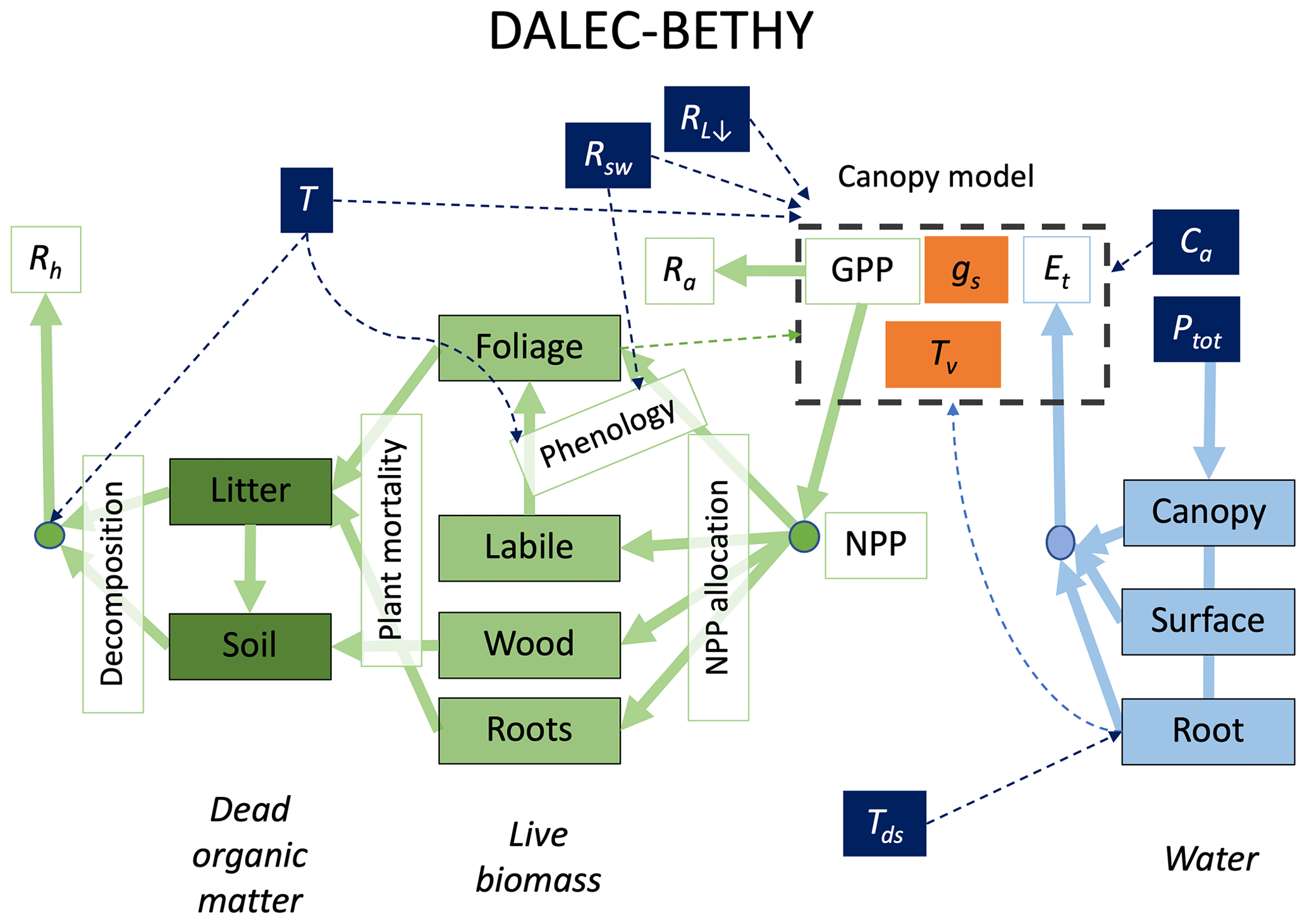
Figure 1 Structure of the DALEC–BETHY coupled model. State variables are in filled boxes: green for carbon, pale blue for water and orange for canopy states of stomatal conductance (g_s) and leaf temperature (T_v). Drivers are shown with white text in dark blue boxes (T: air temperature, T_ds: deep-soil temperature, R_sw: downwelling shortwave radiation, R_L↓: downwelling longwave radiation; P_tot: total precipitation, C_a: CO₂ concentration in air). Fluxes are shown as solid arrows and annotated by open boxes (coloured green for C fluxes and pale blue for water). GPP is gross primary production, NPP is net primary production, R_A is autotrophic respiration, R_H is heterotrophic respiration and E_t is evapotranspiration. Dashed arrows show influences – for example, T and R_sw influence the modelling of phenology.

2 Model description

The D&B model is comprised of three interconnected components: (i) photosynthesis and autotrophic respiration, (ii) energy and water balance, and (iii) carbon allocation and cycling (Fig. 1). The first component comprises processes that lead to the uptake of CO₂ via plant photosynthetic activity (gross primary production, GPP), influenced by temperature, light absorption across the canopy and stomatal control, as well as carbon loss from the respiration of live vegetation (R_A, autotrophic respiration). The remaining carbon flux is then passed as net primary production (NPP = GPP − R_A) to the carbon allocation and cycling component. The energy and water balance component determines the energy input to and output from the canopy in the form of radiative heat, latent and sensible heat transport, taking into account the water balance of the canopy and soil, as well as the rate of water uptake from the roots. Components (i) and (ii) are based on BETHY, and component (iii) is based on DALEC.

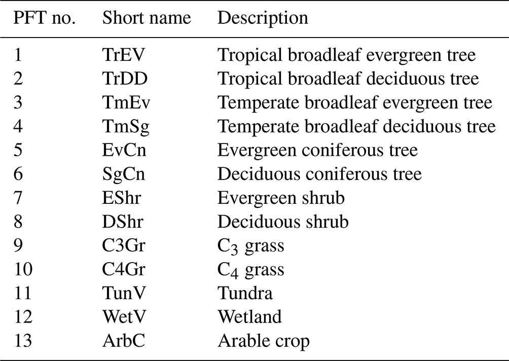
Depending on the domain for which the model is set up, D&B distinguishes between up to 13 plant functional types (PFTs), as shown in Table 1. Each PFT is characterised by a unique set of parameter values. All PFTs use the C₃ photosynthetic pathway, except for PFT 10, for which a separate module for C₄ photosynthesis is used (see Sect. S1.1.1 in the Supplement). Management of arable crops is represented by appropriate parameters for leaf onset and fall, as well as assumptions about a minimum level to which soil moisture is allowed to fall, as an approximation of irrigation (Sect. S1.2.7).

Table 1 Parameter combinations are available for the following plant functional types in D&B.

The fundamental model time step is 1 h. The following components are, however, simulated at a daily time step in order to decrease the computational effort:

• soil water balance,

• canopy water balance,

• snow module,

• the observation operators for VOD and surface soil moisture.

The model simulates several PFTs in sub-grid tiles. Each PFT is simulated separately as if it would cover the full grid cell, with the results rescaled by multiplying them with the grid-cell fraction occupied by the specific tile. Inter-PFT competition for light or water is neglected. A given grid cell can thus comprise several PFTs each with its specific cover fraction.

2.1 Photosynthesis and autotrophic respiration

The C₃ photosynthesis module (Sect. S1.1.1) is based on the biochemical model of photosynthesis by Farquhar et al. (1980). It determines light absorption, light-limited electron transport, CO₂-limited carboxylation rate and the resulting gas exchange of CO₂. Light absorption in the photosynthetically active spectrum is calculated within a two-flux approximation (Sect. S1.1.3), following Sellers (1985). D&B divides the canopy into several vertical layers of equal LAI, the sum of which constitutes the total canopy LAI. In the standard configuration, the number of layers is three. The amount of light absorbed and thus available for photosynthesis is dependent on LAI, statistical leaf orientation (assumed to be isotropic) and leaf single-scattering albedo. Photosynthetic capacity decreases from top to bottom of the canopy, assuming that decreasing levels of daily-average solar radiation drive decreases in leaf nitrogen content and maximum rates of light-limited photosynthesis.

The photosynthesis module further divides GPP into NPP and R_A (Sect. S1.1.2). R_A is modelled as the sum of maintenance and growth respiration (Knorr, 1997). While maintenance respiration is proportional to photosynthetic capacity, growth respiration is proportional to NPP, and it is zero when NPP is negative. Both continually increase with temperature. Negative NPP is also passed on to the C allocation and cycling component, where it leads to the depletion of the labile C pool.

The rate of photosynthesis is first computed under standard conditions without limitation by water availability. This potential photosynthesis rate is translated into an equivalent stomatal conductance, i.e. the stomatal conductance necessary to provide the flow of CO₂ to the leaf interior. This value for stomatal conductance without water limitation is reduced depending on the vapour pressure deficit of the surrounding air and available soil moisture. This modified stomatal conductance, or actual stomatal conductance, then determines actual photosynthesis and, using information from the energy and water balance component, the rate of transpiration.

2.2 Energy and water balance

The energy and water balance component requires the rate of transpiration from the photosynthesis module, due to the tight coupling between water loss through transpiration and CO₂ uptake by leaves. Transpiration (Sect. S1.2.4) is subsequently combined with other evaporative fluxes, namely of intercepted water (canopy evaporation, Fig. 2, Sect. S1.2.3) and from the soil surface (soil evaporation, Sect. S1.2.5), including snow sublimation (Sect. S1.2.7), to derive total evapotranspiration and latent heat flux. Latent heat flux is constrained by the available net radiative energy input, which the model computes separately for the vegetation canopy and the soil (Sect. S1.2.6). Sensible heat flux is computed from the assumption of energy closure from net radiation, latent heat flux and soil heat flux. The model uses incoming shortwave (solar) and longwave (thermal) radiation as input, but it simulates both outgoing radiation components internally, using information on the albedo of the soil background and vegetation (Sect. S1.2.8).

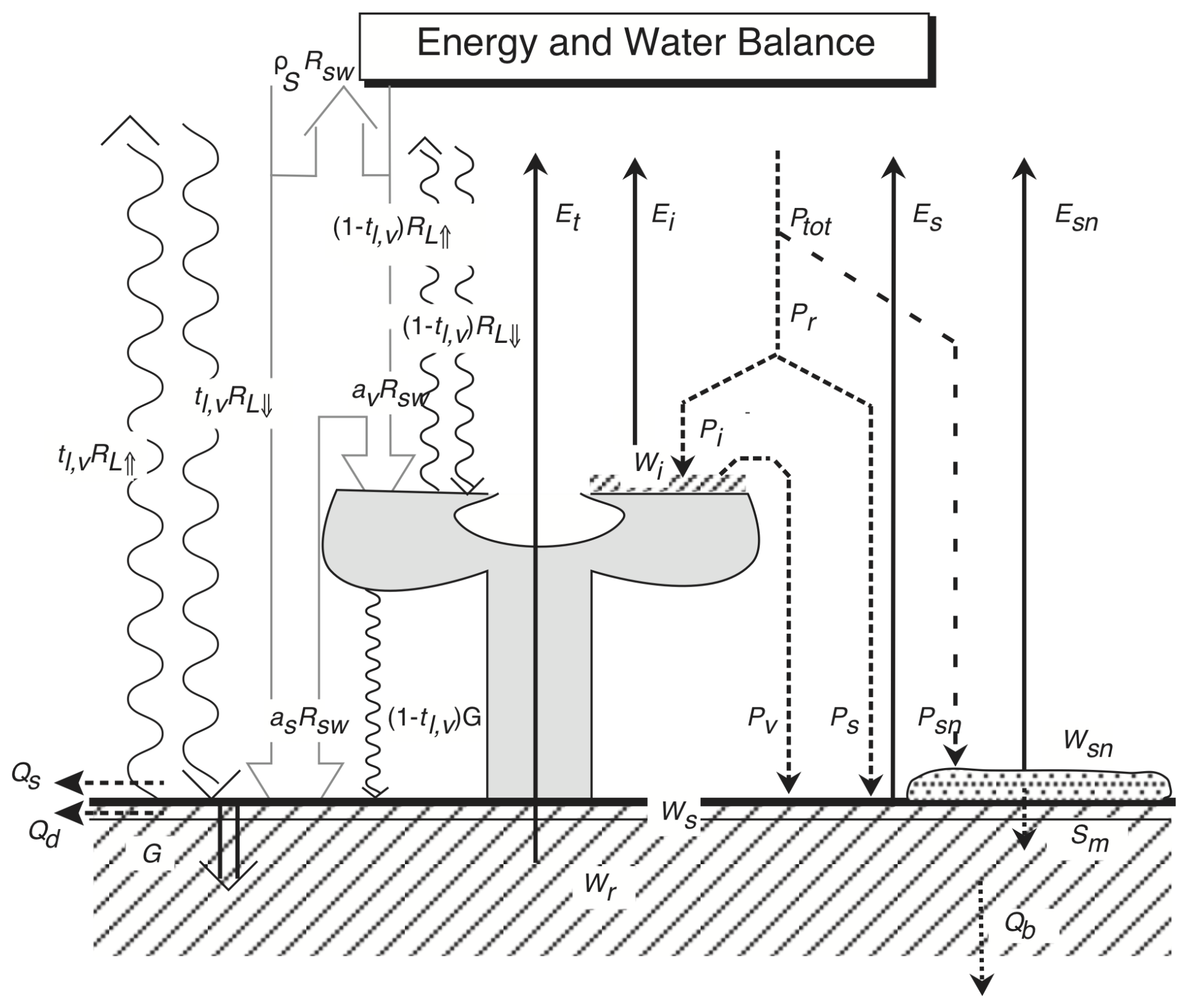
Figure 2 Energy and water balance of the D&B model. a_s: soil absorption of shortwave radiation, a_v: canopy absorption of shortwave radiation, E_i: intercepted-water (canopy) evaporation, E_s: soil evaporation; E_sn: snow evaporation, E_t: transpiration, G: ground heat flux, P_i: intercepted rainfall; P_r: rainfall; P_s rainfall on soil; P_sn: snowfall, P_tot: total precipitation; P_v: throughfall, Q_b: baseflow, Q_d: horizontal drainage, Q_s: surface runoff, $R_{\mathrm{L},\uparrow }$: upwelling longwave radiation, $R_{\mathrm{L},\downarrow }$: downwelling longwave radiation, R_sw: downwelling shortwave radiation, S_m: snowmelt, t_l,v: longwave canopy transmission, W_i: intercepted water amount, W_r: root-zone soil moisture, W_s: surface-layer soil moisture, W_sn: snow amount, and ρ_S: surface reflectance.

Soil evaporation proceeds at the equilibrium rate driven by the soil net radiation from a thin surface layer. This corresponds to a typical depth for which microwave remote sensing can provide soil moisture estimates (Babaeian et al., 2019). Evapotranspiration from the canopy happens as either canopy evaporation from leaf surfaces at the equilibrium rate (Jarvis and McNaughton, 1986) or as transpiration through leaf pores. Precipitation enters either the leaf interception pool or the soil pool (Sect. S1.2.1). Precipitation happens as either snow (Sect. S1.2.7) or rainfall, partitioned into a canopy-interception part, soil infiltration and surface runoff. Soil water drains as subsurface runoff or base flow. Infiltration into the soil (Sect. S1.2.2), runoff, drainage and baseflow (Sect. S1.2.5) are simulated following a new implementation of the variable infiltration capacity approach (Wood et al., 1992), where a thin surface layer has been added to a single root-zone layer (Scholze et al., 2016). The surface soil moisture layer overlaps with the root-zone layer so that the near-surface soil water pool forms part of the root-zone soil water pool (Fig. 2). The former has a nominal depth of 4 cm, the latter has a depth equal to a PFT-specific root depth, d_r (Table S1 in Sect. S1.1.2). Both depths are limited by depth to bedrock. Soil water exiting the root zone downwards is considered subsurface drainage, while there is no upwards water movement from below the root zone. The root-zone soil moisture pool contains all simulated soil water, while the surface layer is added in order to be able to calculate soil evaporation, as well as for diagnostic purposes, accounting for the impact of surface soil moisture on microwave remote sensing.

Once per day around the time of maximum evaporative demand, assumed to be at the hourly time step closest to 13:00 local solar time (Knorr, 1997), the parameters determining actual stomatal conductance are reset to reflect soil water status. To do this, transpiration is simulated as the minimum of a root water supply rate, which increases linearly as soon as soil water exceeds the permanent wilting point, reaching a maximum with soil water at field capacity, and the demand for transpiration. This rate of demand is determined by the potential rate of photosynthesis without water stress computed previously at each time step. Potential photosynthesis is assumed as the rate at a fixed ratio of leaf CO₂ content to atmosphere CO₂ content (0.87 for C₃ and 0.67 for C₄ photosynthesis). Actual photosynthesis and stomatal conductance are then set such that transpiration is downregulated from its potential rate to the rate of maximum root water supply. A supply–demand calculation then determines the rate at which leaf stomata close in response to the water vapour deficit of the surrounding air (See Sect. S1.2.4, Eq. S67).

Finally, the surface reflectance, or background albedo (ρ_S), is affected by soil brightness, surface soil water content and the presence of snow. Vegetation albedo as a function of absorption in the photosynthetically active spectrum, computed in the photosynthesis module, and snow albedo is modelled depending on snow age (Loth et al., 1996; Knorr, 1997).

2.3 Carbon allocation and cycling

The carbon cycle in D&B is expressed as a series of six equations describing the dynamics of six carbon pools. Other than the original DALEC model, D&B employs an hourly time step for allocation, i.e. the same as the time step used by the photosynthesis module. There are four live C pools, namely foliage (fol), wood (wd), fine roots (fr) and a labile (lab) pool which supports foliage expansion. There are two dead organic matter pools, namely litter (lit) and soil organic matter (SOM). The state equations describe the change over time in pool sizes on the basis of C fluxes in and out of the pool. Carbon inputs are all derived originally from NPP. NPP is allocated to each of the four live biomass pools based on fixed site or PFT-specific fractions.

The labile C pool in D&B represents the stored C used to initiate accelerated leaf development at the start of the growing season (Sect. S1.3.1). The phenology scheme parameterises the timing of local bud burst via allocation to leaves from the labile pool based on calibrated climate sensitivity. Leaf development thus depends on the allocation of labile carbon, replenished from NPP, to the leaf carbon pool in addition to direct allocation from NPP. The leaf area index is determined by the conversion of leaf carbon pool size to leaf area by way of fixed values of leaf mass per area.

Losses from fine root (fr) and wood pools (wd) are determined by first-order differential equations, using a decay constant. Biomass dynamics of plant pools are the outcome of NPP allocation and these mortality losses (Sect. S1.3.2). Parameters for the C cycle in D&B use PFT calibrations derived for DALEC using the CARDAMOM model–data fusion approach (Bloom and Williams, 2015). CARDAMOM uses ecological and dynamical constraints to ensure that allometric relationships arising from parameter selection (like emergent root / shoot ratios) are kept within ecologically realistic bounds. By calibrating DALEC using both LAI and woody biomass data, a constraint is placed on relevant model parameters to match the measured biomass of these plant organs.

Losses from the fine-root pool replenish the litter pool, added by strongly periodic inputs linked to leaf senescence, while wood directly feeds SOM. The litter pool either decays to CO₂ via heterotrophic respiration or is decomposed to the SOM pool. Mineralisation of both SOM and litter C pools by heterotrophic respiration thus results in further CO₂ fluxes. Total ecosystem respiration (TER) is determined by the sum of autotrophic growth and maintenance respiration and mineralisation of dead organic matter (lit or SOM), creating a flux of heterotrophic respiration. Following the procedure used for DALEC, the prior parameter values of the carbon allocation and cycling component are set through a regional-scale calibration procedure, as described in Sect. S1.3.3.

3 Observation operators

The task of an observation operator is to simulate the equivalent of an observation from the model's state variables. This includes the simulation of the variable that is retrieved at the time when it was observed and over the footprint of the observations, i.e. the source area of the signal measured by the respective instrument (Kaminski and Mathieu, 2017). In this paper, we will present the simulation of four data streams, namely FAPAR, SIF, L-band VOD and near-surface soil moisture, and then confront model simulations with local measurements. Of the four data streams, FAPAR and surface soil moisture are internally calculated.

3.1 Fraction of absorbed photosynthetically active radiation (FAPAR)

FAPAR is a measure of the capacity of terrestrial vegetation to absorb sunlight in the visible spectrum, i.e. that part that can be utilised for photosynthesis. It is defined as the amount of photosynthetically active radiation (PAR) absorbed by functioning green leaves divided by the total incoming PAR. FAPAR is calculated within the two-flux canopy radiative transfer scheme (Sect. S1.1.3) required for the calculation of GPP (Sect. 2.1). However, due to the dependence of FAPAR on solar zenith angle, it is necessary to take into account the solar zenith angle at time of observation. Therefore, the observation operator for FAPAR utilises FAPAR calculations performed within the model's photosynthesis component at the times and dates when model and observations solar zenith angles match.

3.2 Solar-induced fluorescence (SIF)

Strictly speaking, the canopy-level solar-induced chlorophyll fluorescence, or SIF, is a measure not of the photosynthetic rate as such but of the amount of radiation absorbed by the leaf and not used for the purpose of photosynthesis. Some of that surplus radiation is re-emitted as fluorescent light as part of a coping mechanism of the photosynthetic system. Under normal field conditions, however, SIF can often be used as an indication of photosynthetic activity, as opposed to FAPAR, which only characterises the photosynthetically active light that is potentially available (Porcar-Castell et al., 2014; Mohammed et al., 2019).

To calculate SIF, we use the formulation of Gu et al. (2019). This choice is motivated by the direct link to the photosynthesis routines and the relatively parsimonious implementation, which fits with the modelling strategy adopted here. The canopy layer SIF, S_n, is given by

$$\begin{array}{}\text{(1)}& S_n=s_{\mathrm{SIF}}{J}_n{\displaystyle \frac{\mathrm{1}-{\mathit{\psi }}_{\mathrm{PSIImax}}}{q_{\mathrm{L}}{\mathit{\psi }}_{\mathrm{PSIImax}}(\mathrm{1}+k_{\mathrm{DF}})}},\end{array}$$

where J_n is the electron transport in canopy layer n (Eq. S8), ψ_PSIImax is the maximum photochemical quantum yield of photosystem II, q_L is the fraction of open photosystem II reaction centres and k_DF is the ratio of the first-order rate constants for heat dissipation and fluorescence. We take the values prescribed by Gu et al. (2019). Note that the original equation in that paper also has a term for the photon escape probability from the canopy. In D&B, this is calculated explicitly by the layered two-stream model (Sect. S2) and hence is not required here. As an extension to the model by Gu et al. (2019) in view of the anticipated calibration in a data assimilation scheme, we further introduce the scaling factor s_SIF, which compensates for large uncertainties in (1) the values of the three constants (ψ_PSIImax, q_L and k_DF) and (2) the spectral conversion that is described below. We set the prior value of s_SIF to 1.

SIF produced by the D&B model via the layered two-stream model described in Sect. S2 has native units of mol m⁻² s⁻¹. It represents the total flux of photons into the hemisphere above the canopy for all wavelengths. Satellite measurements and in situ observations, however, are typically recorded in energy flux units per steradian per nanometre of the SIF spectra, e.g. W m⁻² s⁻¹ nm⁻¹ sr⁻¹. To convert from molar to energy units, we apply the molar form of the Planck equation, providing energy per mole of photons: $e=ahc/{\mathit{\lambda }}_{\mathit{\varphi }}$, where a is Avogadro's number, 6.023×10²³; h is the Planck constant, $\mathrm{6.626}\times {\mathrm{10}}^{-\mathrm{34}}$ m² kg s⁻¹; c is the speed of light, 3.0×10⁸ m s⁻¹; and λ_ϕ is the wavelength of the SIF photons in metres.

We convert to steradians by using a constant factor of $\frac{\mathrm{1}}{\mathrm{2}\mathit{\pi }}$, which assumes that the emittance of SIF from the top of the canopy is isotropic, and finally we weight by the relative strength of emissions at λ_ϕ compared to a reference SIF spectrum:

$$\begin{array}{}\text{(2)}& w={\displaystyle \frac{E\left({\mathit{\lambda }}_{\mathit{\varphi }}\right)}{{\sum }_{i}E\left({\mathit{\lambda }}_{\mathit{\varphi },i}\right)}},\end{array}$$

where E is the SIF emission spectrum of arbitrary units. Hence,

$$\begin{array}{}\text{(3)}& {\mathrm{SIF}}^{\prime }=\mathrm{SIF}{\displaystyle \frac{ew}{\mathrm{2}\mathit{\pi }}},\end{array}$$

where SIF has units of mol m⁻² s⁻¹, and SIF^′ has units of W m⁻² s⁻¹ sr⁻¹ nm⁻¹.

For the present study, we use a SIF emission spectrum observed at the Hyytiälä site in Finland (Magney et al., 2019). The SIF spectrum was measured for four Scots pine trees at a light level of 1200 µmol m⁻² s⁻¹ and then averaged.

3.3 Vegetation optical depth (VOD)

VOD is essentially a parameter describing the attenuation of microwave radiation at some wavelength due to the presence of vegetation. It depends on the dielectric properties (due to water content, temperature and chemical composition) as well as the structure and geometry of the vegetation and sensor properties (e.g. wavelength, polarisation). Due to the relatively static nature of vegetation structure, dynamics of VOD are generally attributed to changes in aboveground biomass and water content (Ulaby and Wilson, 1985; Konings et al., 2019). It is measured within the microwave spectrum with passive instruments, using the black-body radiation of the surface in the microwave domain, or active instruments such as scatterometers or synthetic aperture radars.

Common retrieval methods may extract both the surface soil moisture and VOD simultaneously from satellite remote sensing data, provided enough measurements are performed. For example, the SMOS (Kerr et al., 2010) retrieval algorithm (Kerr et al., 2012) is based on the so-called τ−ω formulation for the vegetation contribution (Kirdiashev et al., 1979; Mo et al., 1982) of the microwave signal, where VOD is denoted by τ, the perpendicular vegetation optical depth (Wigneron et al., 2007, 2010).

Here, however, we compare simulations to locally measured L-band passive VOD measurements. Due to the local setup where separate sensors are placed above and below the canopy (see Sect. S3.6), it is possible to measure VOD directly without having to solve for soil moisture simultaneously.

We use a semi-empirical formulation for L-band VOD, expressed as

$$\begin{array}{}\text{(4)}& {\mathit{\tau }}_{\mathit{\lambda }}=f\left(T\right)(l_{\mathrm{wd}}{C}_{\mathrm{wd}}+l_{\mathrm{fol}}{C}_{\mathrm{fol}})(l_{\mathrm{s}}{f}_{\mathrm{soil}}+l_{\mathrm{f}}{f}_{\mathrm{E}}+l_{\mathrm{0}}),\end{array}$$

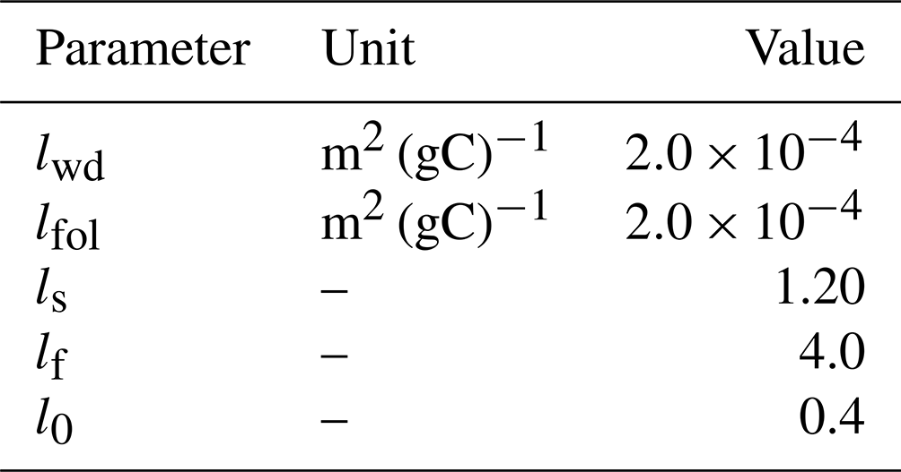
where the subscript λ denotes its wavelength dependence; C_fol and C_wd are the leaf and woody biomass pools, respectively (see Sect. S1.3.2); f_soil (Eq. S92) is fractional plant-available soil water content; and

$$\begin{array}{}\text{(5)}& f_{\mathrm{E}}=E_{\mathrm{t}}/E_{\mathrm{t},\max },\end{array}$$

i.e. the ratio of actual to potential transpiration (see Eq. S61). f_soil describes slow changes in the plant's hydrological status, hence multiplied by parameter l_s, and f_E describes fast changes, hence multiplied by parameter l_f. The other empirical parameters are l₀, l_wd for dependence on woody biomass and l_fol for dependence on leaf biomass. We note that the five empirical parameters are wavelength-dependent; for convenience, we refrain from adding an additional subscript λ.

Following Schwank et al. (2021), we include an explicit temperature dependency in the form of

$$\begin{array}{}\text{(6)}& f\left(T\right)=\mathrm{0.25}+\mathrm{0.75}/(\mathrm{1}+e^{-\mathrm{0.5}(T+\mathrm{3})}),\end{array}$$

which approximates the theoretically derived behaviour around the freezing point, with T being 2 m air temperature. This formulation can be used across a range of microwave wavelengths, using different parameter values in each case. The second multiplicative factor in Eq. (4) is an empirical linear expression using both woody and foliar biomass with the assumption that VOD will be zero if no biomass is present. The third multiplicative factor describes how the water status of the vegetation modifies this expression. This last one also contains a constant factor, l₀>0, because we expect positive VOD even if vegetation water stress is at its maximum.

In this contribution, we apply it to passive L-band microwave measurements. The values of the parameters for the empirical VOD observation operator, shown in Table 2, were selected such that the model reproduces a reasonable fit to L-band observations from SMOS over the Sodankylä and the Majadas de Tiétar sites.

Table 2 Parameters for the empirical observation operator for L-band VOD.

3.4 Near-surface soil moisture

In the D&B model, near-surface soil moisture is represented by an explicitly modelled thin surface soil moisture layer, with a depth of 4 cm, unless the depth to bedrock indicates a lower value. It is therefore a state variable in the model's soil water component and is described in detail in Sect. 2.2. This surface layer therefore serves a dual purpose: first to simulate soil evaporation and second to diagnose a variable that can be retrieved from satellite observations. Near-surface soil moisture is usually available from passive microwave measurements when retrieved simultaneously with VOD (Sect. 5.3). These retrieval algorithms explicitly separate the contributions to the microwave signal that come either from the vegetation (VOD) or from the soil (surface soil moisture).

4 Model evaluation

We first present an evaluation of the D&B model on its own, followed by an evaluation of the model together with the observation operators for the four data streams of FAPAR, SIF, L-VOD and surface soil moisture. The methods used to derive the driving data for the model as well as those of the measurements undertaken for driving and evaluating the model are described in Sect. S3.

4.1 Study sites

The D&B model is run for two study sites with widely varying climate, one representing a boreal forest – Sodankylä in Finland, a class 1 site of the Integrated Carbon Observation System (ICOS) network (Rebmann et al., 2018) – and the other representing a temperate-savannah ecosystem – Majadas de Tiétar in Spain, also an ICOS network site. The Sodankylä Scots pine forest site (67°21^′44.6^′′ N, 26°38^′18.9^′′ E) is situated 100 km north of the Arctic Circle (Thum et al., 2007; Honkanen et al., 2023). It also has an understorey of evergreen ericaceous shrub (mostly blueberry) as well as lichen and mosses. The soil is characterised as predominantly sand (clay / silt / sand / stone ratios for different depths are given; 0–10 cm: 0.5 % / 6.0 % / 88.1 % / 5.4 %, 10–20 cm: 0.3 % / 4.1 % / 93.5 % / 2.1 %, 20–40 cm: 0.2 % / 2.8 % / 91.9 % / 5.1 %).

The Majadas de Tiétar site is a Mediterranean open woodland of evergreen holm oak in western Spain (39°56^′24.68^′′ N, 5°45^′50.27^′′ E; Wang et al., 2016; El-Madany et al., 2018). The soil (Nair et al., 2020) contains an upper sandy layer (5 % clay, 20 % silt, 75 % sand, 20 cm deep) underlain by a clay layer (30 to 60 cm depth, no information for 20 to 30 cm).

4.2 Model setup

We use locally observed data to drive the model (see Sect. S3.1). C_a is set to a uniform value of 405 ppm, i.e. $C_{\mathrm{a}}=\mathrm{405}\times {\mathrm{10}}^{-\mathrm{6}}$ mol(CO₂) mol(air)⁻¹, which is approximately the annual mean value at Mauna Loa, Hawaii, centred around the beginning of 2017 (NOAA, 2024). Model runs are with a priori values of the parameters for all modules and observation operators. Initial water content of the soil was set to 50 % of field capacity. Simulations for the first 2 calendar years were discarded to avoid model biases due to initial conditions of the water balance and short-lived carbon pools. The fractional vegetation cover is set to f_c=1 for both sites.

For Sodankylä, the model simulation was run for the period 1 January 2009 to 31 December 2021, with two PFTs: evergreen coniferous forest (PFT 5, 67 % of ground area) and evergreen shrub (PFT 7, 33 %). Measured soil temperature as model input is for 1 m depth. The soil texture class is “medium/coarse” (cf. Sect. S1.2.5, Table S4), following the classification of the global soil texture data set by Zobler (1986). Parameter and initial values related to carbon turnover are set according to Table S6 (Sect. S1.4).

For Majadas de Tiétar, the simulation is for 1 April 2014 to 31 December 2021. We assume the site area to comprise C₃ grass (PFT 9, 80 % of ground area) and temperate evergreen trees (PFT 3, 20%). The model is driven by soil temperature measured at 80 cm depth averaged between four locations, two in open grassland and two under a tree canopy. The soil texture class is medium. Parameters and initial values related to carbon turnover are set according to Table S7.

4.3 Evaluation approach

The D&B model is compared against eddy covariance data of carbon and energy fluxes, locally observed radiation balance, and (in the case of the boreal site) snow depth. This is a first evaluation of the model with its prior parameterisation, and its purpose is to assess whether the model is able to reproduce measurements with a reasonable degree of realism. The role of the in situ observations is to serve as an independent evaluation data set.

We compare multi-year time series by showing the following values for both observations and model simulations: $f_j,f_j^{\min },f_j^{\max }$, where

$$\begin{array}{}\text{(7)}& f_j={\displaystyle \frac{\mathrm{1}}{n}}\sum _{i=\mathrm{1}}^{n}f(i,j),\end{array}$$

and f is the flux of interest, i counts the n simulation years used for this analysis, and j is the day within the year (1 January to 31 December). $f_j^{\min }$ and $f_j^{\max }$ denote the minimum and maximum across the n values $\mathit{\left\{}f\right(\mathrm{1},j),\mathrm{\dots },f(n,j\left)\mathit{\right\}}$, respectively. We also show the multi-year mean for both observations and models as

$$\begin{array}{}\text{(8)}& \stackrel{\mathrm{‾}}{f}={\displaystyle \frac{\mathrm{1}}{nm}}\sum _{i=\mathrm{1}}^n\sum _{j=\mathrm{1}}^{m}f(i,j),\end{array}$$

where m is the number of days per year. In addition, we provide the following metrics: root-mean-square error (RMSE) of daily,

$$\begin{array}{}\text{(9)}& {\mathrm{RMSE}}_{\mathrm{daily}}={\displaystyle \frac{\mathrm{1}}{nm}}\sqrt{\sum _{i=\mathrm{1}}^n\sum _{j=\mathrm{1}}^m{\left[f_{\mathrm{mod}}(i,j)-f_{\mathrm{obs}}(i,j)\right]}^{\mathrm{2}}},\end{array}$$

and annual values,

$$\begin{array}{}\text{(10)}& {\mathrm{RMSE}}_{\mathrm{annual}}={\displaystyle \frac{\mathrm{1}}{n}}\sqrt{\sum _{i=\mathrm{1}}^n{\left({\stackrel{\mathrm{‾}}{f}}_{i,\mathrm{mod}}-{\stackrel{\mathrm{‾}}{f}}_{i,\mathrm{obs}}\right)}^{\mathrm{2}}},\end{array}$$

with ${\stackrel{\mathrm{‾}}{f}}_i$ denoting annual average fluxes for year i for either simulations (mod) or observations (obs), as well as explained variance (r²) at daily and annual timescales:

$$\begin{array}{}\text{(11)}& r_{\mathrm{daily}}^{\mathrm{2}}={\displaystyle \frac{{\sum }_{i=\mathrm{1}}^n{\sum }_{i=j}^m{\left(f_{\mathrm{mod}}(i,j)-{\stackrel{\mathrm{‾}}{f}}_{\mathrm{obs}}\right)}^{\mathrm{2}}}{{\sum }_{i=\mathrm{1}}^n{\sum }_{i=j}^m{\left(f_{\mathrm{obs}}(i,j)-{\stackrel{\mathrm{‾}}{f}}_{\mathrm{obs}}\right)}^{\mathrm{2}}}},\end{array}$$

and

$$\begin{array}{}\text{(12)}& r_{\mathrm{annual}}^{\mathrm{2}}={\displaystyle \frac{{\sum }_{i=\mathrm{1}}^n{\left({\stackrel{\mathrm{‾}}{f}}_{i,\mathrm{mod}}-{\stackrel{\mathrm{‾}}{f}}_{\mathrm{obs}}\right)}^{\mathrm{2}}}{{\sum }_{i=\mathrm{1}}^n{\left({\stackrel{\mathrm{‾}}{f}}_{i,\mathrm{obs}}-{\stackrel{\mathrm{‾}}{f}}_{\mathrm{obs}}\right)}^{\mathrm{2}}}}.\end{array}$$

Carbon fluxes are gross primary production (GPP), total ecosystem respiration (TER) and net ecosystem exchange (NEE = TER − GPP). NEE is defined as going from the vegetation to the atmosphere, i.e. positive values denote a flux of CO₂ towards the atmosphere. Energy fluxes are latent heat flux (LHF) and sensible heat flux (SHF), with the addition of net radiation, which is the balance of incoming minus outgoing solar and thermal radiation fluxes. Both carbon and energy fluxes as well as net radiation are measured over a representative area of each ecosystem, consisting of different PFTs.

For the purpose of calculating the above statistics, we used the 6-year period from 2016 to 2021 for both sites. We additionally use snow depth measurements from the period 2011 to 2021 for validation at the Sodankylä site. Biomass and soil carbon measurements, also at the Sodankylä site, were taken in 2011 and are compared to mean values of the simulations from 2011 to 2021 (Sodankylä) or from 2016 to 2021 (Majadas de Tiétar). See Sect. S3 for details of measurement methods.

4.4 Evaluation at a boreal-forest site: Sodankylä

At the boreal-forest site (Fig. 3), measurements show a markedly smaller amplitude of the annual cycle of carbon fluxes (NEE) than the model. While in the springtime there is a reasonable agreement with an initial rapid increase in the magnitude of NEE, carbon loss during the winter as well as carbon uptake during summer and early autumn are clearly larger for the model. Between day of year (DOY) 200 and 260 (mid-July to mid-September), the discrepancy in NEE is associated with an underestimation by the model of respiration (TER) and an overestimate of GPP. Not surprisingly, GPP agrees well during the winter as it is well constrained due to the lack of light and low temperatures, but TER is generally higher for the model. There is also a conspicuous phase shift of TER between the two curves, with measurements showing TER peaking much later, while the phases of GPP agree reasonably.

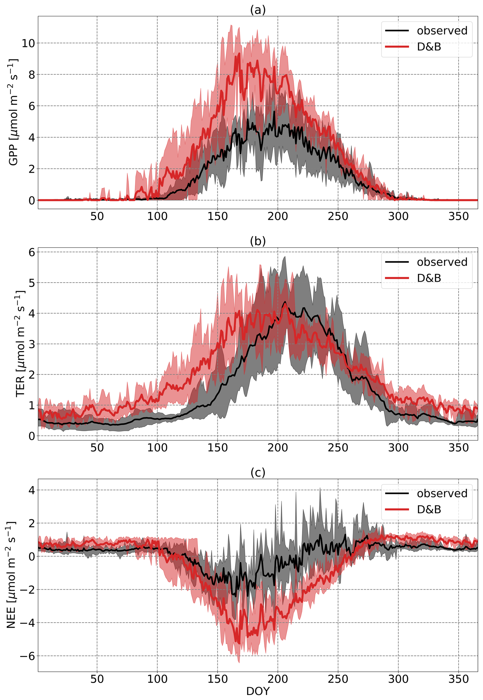
Figure 3 Annual cycles of daily (a) GPP, (b) TER and (c) NEE at Sodankylä, averaged over the years 2016 to 2021. Black line is observation based on eddy covariance data; the red line is D&B. The shaded areas represent the ranges of the observed and simulated daily cycles over the period.

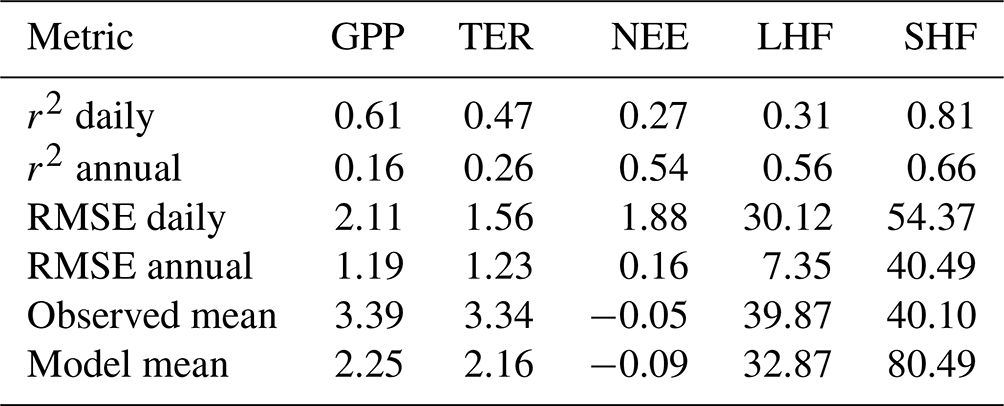
For the energy flux evaluation (Fig. 4), what stands out is the good agreement between modelled and simulated SHF, except for the spring (ca. DOY 50 to 100), where observations exceed simulations. LHF is also well matched during the summer (ca. DOY 120–260). Since in the model energy balance is exactly fulfilled, we would expect an equally good match for the net energy input (i.e. net radiation minus ground heat flux; cf. Eqs. S124, S127) if the energy balance is also fulfilled for the observations. However, observations during the summer period are systematically lower than simulations. Therefore, we attribute the mismatch in net radiation during the summer to a lack of energy closure of the eddy covariance measurements. However, for the winter months, SHF is in good agreement, but both net energy input and LHF show systematically higher values for the model; hence, there is no evidence of a lack of energy closure for the measurements. The difference might thus be mostly due to an overestimate by the model.

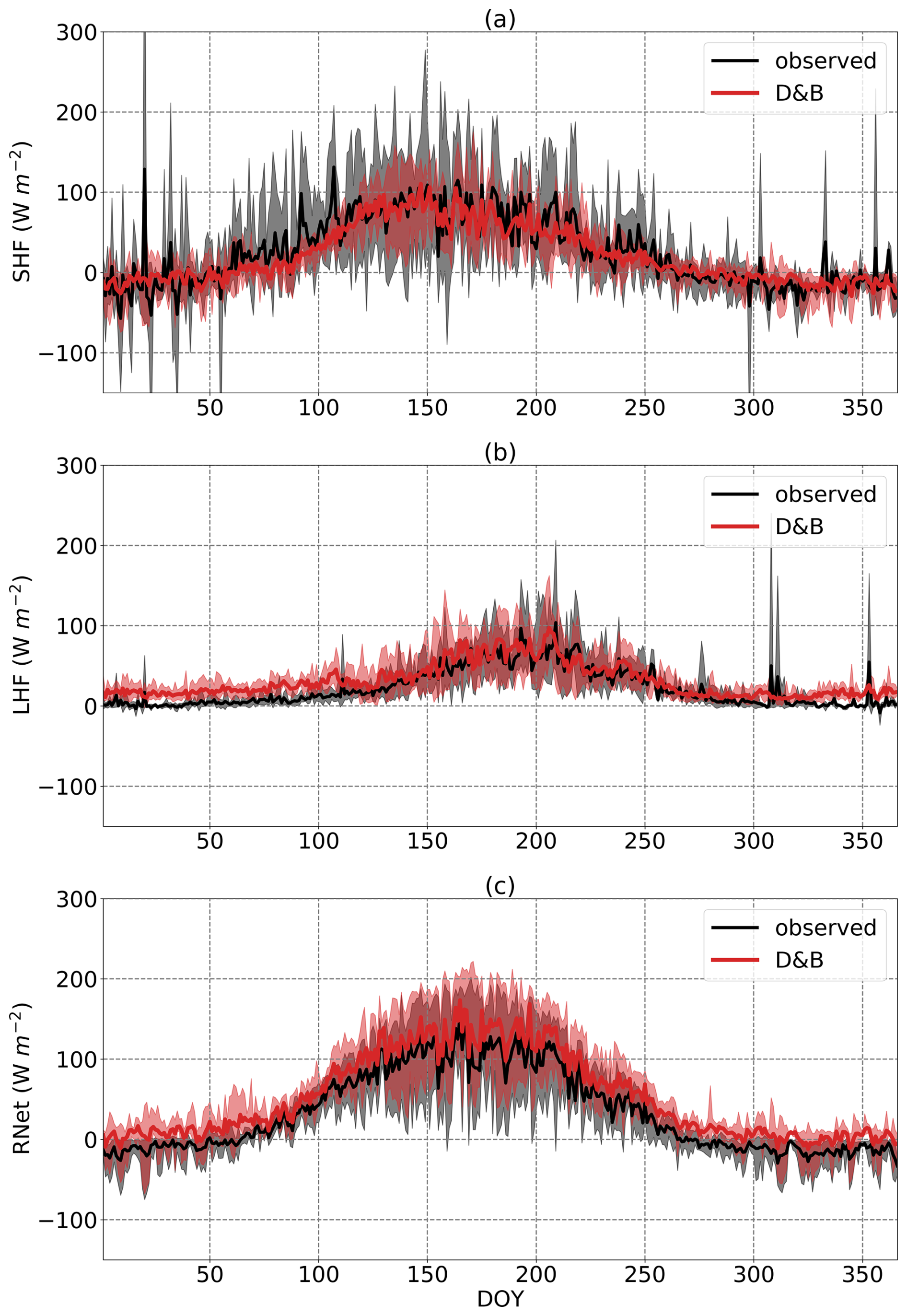
Figure 4 Annual cycles of daily (a) sensible heat flux, (b) latent heat flux and (c) net radiation minus ground heat flux at Sodankylä, averaged over the years 2016 to 2021. The shaded areas represent the ranges of the observed and simulated daily cycles over the period.

Another noteworthy period is the wintertime, where the model produces slightly negative SHF and at the same time overestimates LHF compared to observations. Both deviations just about cancel each other, and there does not seem to be an issue with energy closure for the observations.

Snow depth observations taken from within the forest and simulated snow depth for the evergreen conifer tree PFT agree generally very well (Fig. 5). The model tends to somewhat underestimate the observations, especially at the time of snowmelt, where snow depth is receding, but the differences are small and the comparison favourable, in particular when noting the good agreement in interannual variations. The peak winters with the highest values (e.g. the winter 2019/2020) are also well reproduced.

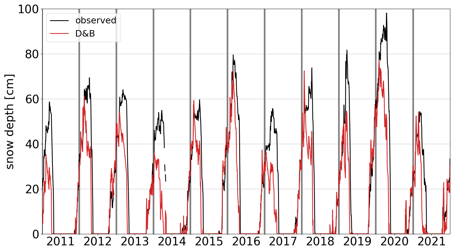
Figure 5 Daily observed (black) and simulated (red) snow depth at Sodankylä for the years 2011–2021. Simulated snow depth is for the evergreen conifer PFT only.

On an annual average basis, modelled NEE shows a small carbon sink with NEE equal to −197 gC m⁻² yr⁻¹, against a smaller source in magnitude for the measurements of +34 gC m⁻² yr⁻¹ (values given in Table 3 converted from molar units). GPP is 534 gC m⁻² yr⁻¹ when observation-derived against 927 gC m⁻² yr⁻¹ for the model. In contrast to the mean, the explained variance, r², is not sensitive to the absolute magnitude of the fluxes, and since the phases agree well (Fig. 3), it is not surprising that it shows a very high value of 0.87 for GPP at the daily time step. For TER, however, due to the phase shift previously discussed, we find a lower value (r²=0.69). The value of r² for NEE is smaller than for GPP and TER, as we would expect, because NEE is the difference of two larger fluxes and has therefore a much smaller magnitude. Let us assume that the true temporal average of NEE is zero, while each (the model and the measurements) reproduce a temporal average of GPP equal to temporal average of TER but with some temporal noise added. This noise might be due to measurement or model error, but it is uncorrelated between model and measurements. In this case, we would expect the model–measurement correlation for NEE to be zero. However, correlation between modelled and measured GPP or TER could still be substantial due to coinciding temporal variations shorter than the averaging period.

Table 3 Metrics for the different variables simulated at Sodankylä for the period January 2016 to December 2021. RMSE: root-mean-square error. Units: µmol m⁻² s⁻¹ (gross primary production, GPP; total ecosystem respiration, TER; net ecosystem exchange, NEE), W m⁻² (latent heat flux, LHF; sensitive heat flux, SHF) and centimetre (cm, snow depth).

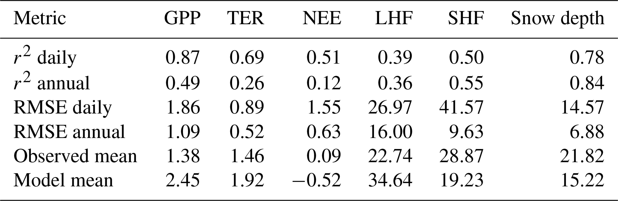
The value of the annual r² in Table 3 captures exclusively interannual variations, and the values are much smaller than derived on the basis of daily averages. It appears that the model only partially reproduces the observation-derived interannual variability, especially for NEE. Note, however, that the number of data points is only six. RMSE for GPP and NEE on a daily basis is similar to the annual mean GPP, likely due to day-to-day variations in the measurements not being captured by the model.

Over all seasons, the model shows much higher LHF than the measurements but much lower SHF (Table 3). The difference comes almost entirely from the winter and spring seasons, as noted when discussing Fig. 4. The r² values are also significantly smaller for energy than for carbon fluxes (Table 3) due to the seasonally varying model–observation differences, which create differing seasonal cycles between the two. By contrast, snow depth shows a very high r² at both the daily and annual timescales, as is apparent from Fig. 5.

Modelled carbon pools differ substantially from locally derived values: the mean and standard deviation of total soil organic carbon found was 3.70 ± 0.16 kgC m⁻², against a model-based estimate of 38.7 kgC m⁻². It appears that the model underestimates the turnover time of the slowest soil carbon pool. The observed aboveground biomass at the site was 37.3 t ha⁻¹ against a model estimate of 62.5 t ha⁻¹, assuming 50 % carbon content of dry mass and 85 % of woody biomass above ground (Helmisaari et al., 2002).

4.5 Evaluation at a temperate-savannah site: Majadas de Tiétar

The seasonal course of carbon exchanges at the temperate-savannah site (Fig. 6) is characterised by a pronounced springtime net carbon uptake and a prolonged period of carbon loss during the summer and autumn. However, the strength of the spring draw-down (ca. DOY 50 to 150) derived from the observations is much lower than the model-derived one. For the remaining seasons, model and observed NEE largely agree in terms of magnitude and timing, except for pronounced fluctuations in the measured NEE flux during summer and autumn that are not reproduced by the model. Such fluctuations are also found in the observation-derived TER flux. The discrepancy in the spring draw-down appears to be the result of a model overestimate of GPP combined with an underestimate of TER.

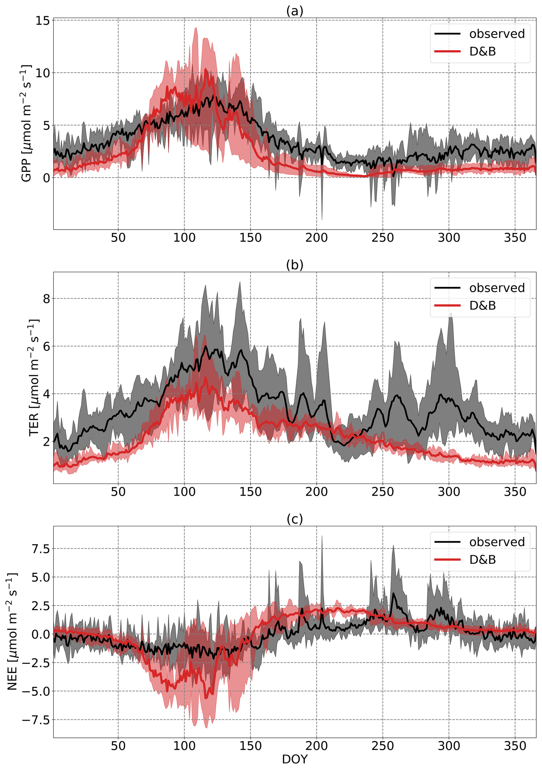
Figure 6 Annual cycles of daily (a) GPP, (b) TER and (c) NEE at Majadas de Tiétar, averaged over the years 2016 to 2021. Black line is observations based on eddy covariance data, and the red line is D&B. The shaded areas represent the ranges of the observed and simulated daily cycles over the period.

If we consider the climate of the site, with hot and dry summers, cool winters, and a winter rainfall maximum, we can assume that the most favourable growth conditions happen in the spring, where we indeed find the largest net CO₂ uptake rate in both model and observations. Under those springtime conditions, however, the model predicts a higher GPP than the observation-based value but a lower GPP value for the remaining seasons where growth is limited in either temperature and light (winter/autumn) or water (summer/autumn). In other words, compared to the observations, the model overpredicts GPP under favourable conditions but underpredicts GPP under conditions of GPP limitations – by way of dry conditions in the summer, low light levels in the autumn and temperature during winter. We thus find that the model likely overestimates moisture limitation, as well as other GPP limiting factors, while overestimating photosynthetic capacity.

On an annual basis (Table 4), simulated GPP (844 gC m⁻² yr⁻¹) is generally smaller compared to the observation-derived estimate (1283 gC m⁻² yr⁻¹). The same also applies to TER (814 gC m⁻² yr⁻¹ vs. 1264 gC m⁻² yr⁻¹ derived from eddy covariance measurements). Net flux (mean NEE) is small and agrees well (−30 vs. −19 gC m⁻² yr⁻¹ for model vs. observations). In contrast to Sodankylä, r² for the annual values shows that the interannual variability of NEE is reproduced well, in fact better than that for the components GPP and TER. However, daily r² is much lower for NEE than for GPP or TER, due to the different shape of the seasonal cycle of the model, showing a pronounced spring draw-down, as already discussed. RMSE values of GPP and TER on a daily basis are similar in magnitude to the modelled ones but less than the observed mean, while annual RMSE for NEE is remarkably low. While the high r² suggests that the model reproduces the interannual variability of the net carbon fluxes well for this site, the combination of rather high RMSE and similar observed means suggests that day-to-day variations are less well captured.

Table 4 Metrics for the different variables simulated at Majadas de Tiétar for the period January 2016 to December 2021. RMSE: root-mean-square error. Units: µmol m⁻² s⁻¹ (gross primary production, GPP; total ecosystem respiration, TER; net ecosystem exchange, NEE), W m⁻² (latent heat flux, LHF; sensitive heat flux, SHF).

As far as the energy balance is concerned, we find a similar result for Majadas de Tiétar (Fig. 7) compared to the boreal-forest site: net energy input (net radiation minus ground heat flux) agrees very well between model and observations, but there is a rather large overestimate by the model of the sensible heat flux, albeit with a very similar shape of the seasonal cycle (r²=0.81, SHF daily, Table 4). For most of the year, except for a pronounced summer decline for the model but not for the observations, LHF agrees well. This is likely related to the model's pronounced underprediction, compared to the observations, of GPP, resulting in a lower transpiration flux through more pronounced stomatal closure and thus also lower LHF. Given the strict energy closure for the model, if net energy input and LHF agree between model and measurements, then SHF should also agree. However, while the model has an exact energy closure, the data apparently do not. For instance, at the start of the years until ca. DOY 130, net radiation and LHF agreement suggests an imbalance in the observations starting close to zero at the start of the year and increasing to around 40 W m⁻². During the summer season, the model overestimates SHF by around 100 W m⁻², but underestimates LHF by only around 60 W m⁻², while net radiation agrees, which also suggests a deviation from energy closure of around 40 W m⁻². This has again to be taken into account when evaluating the model.

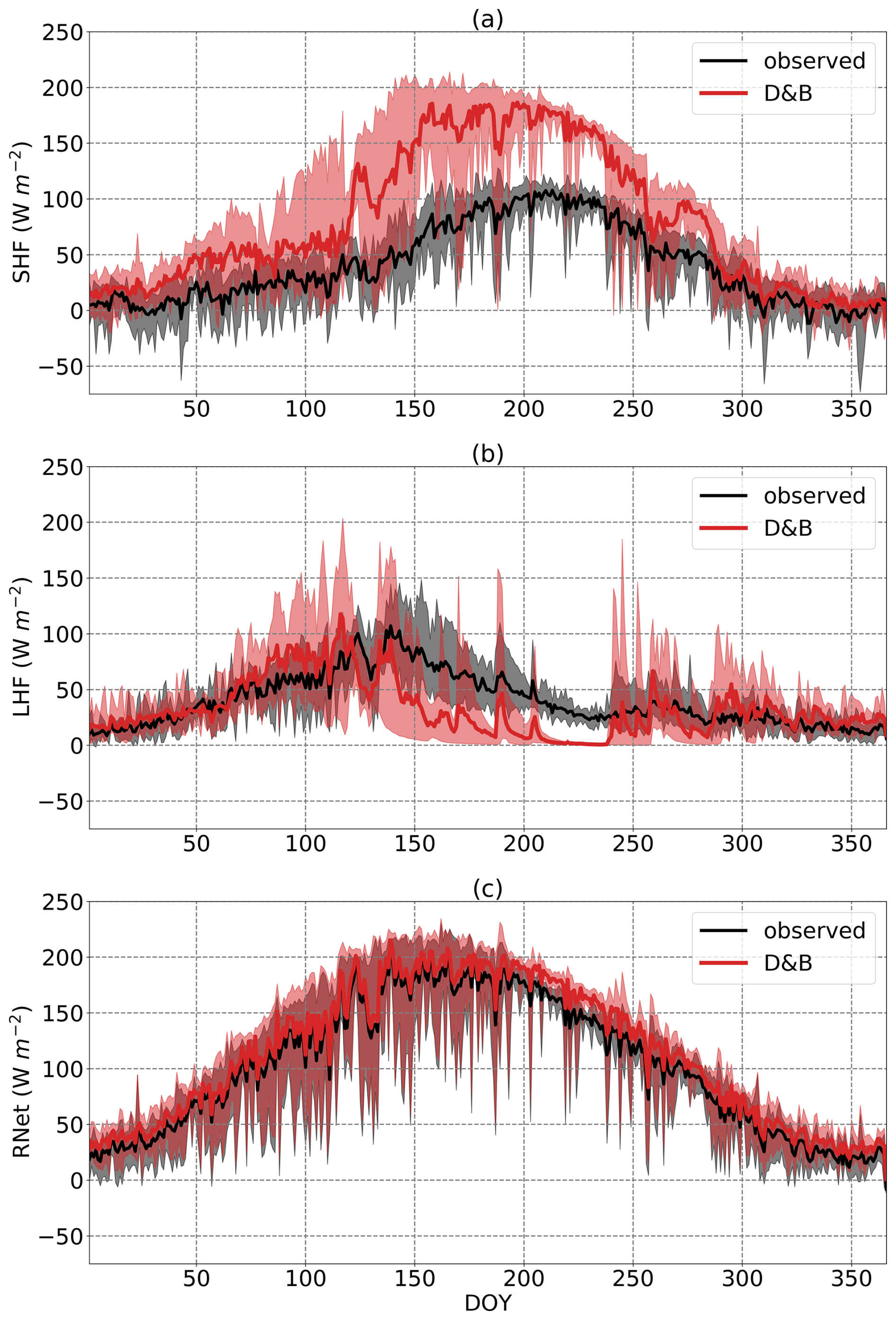
Figure 7 Annual cycles of daily (a) sensible heat flux, (b) latent heat flux and (c) net radiation minus ground heat flux at Majadas de Tiétar, averaged over the years 2016 to 2021. The shaded areas represent the ranges of the observed and simulated daily cycles over the period.

On average (Table 4), the model slightly underestimates LHF but overestimates SHF by close to a factor of 2. For both LHF and SHF, we find high values for r² based on annual averages, and a very small value for annual RMSE for LHF, which suggests that the model, apart from a general overestimate of LHF, simulates interannual variability of energy fluxes reasonably well, with the caveat that only 6 full years are being considered here.

5 Evaluation of observation operators

5.1 Evaluation of FAPAR simulations

The simulations at the Sodankylä site showed larger FAPAR values during the summer than the observations (Fig. 8), with a pronounced seasonal cycle. We find this to be a robust feature of the simulations (not shown). By contrast, observed values stay at approximately the same level during the observation period, with some larger values during the autumn. The values of the observed FAPAR match the expected behaviour of the largely aseasonal evergreen canopies of the PFTs for the boreal region. The pronounced seasonal cycle of FAPAR in the model runs corresponds to a seasonal cycle in the LAI of the model. The modelled LAI behaviour results from calibration using Copernicus LAI time series which have a strong (and unexpected) seasonality. By contrast, measured FAPAR shows only weak signs of seasonality, such as a very slight increase between DOY 170 and 200. There is, however, a cluster of elevated measured FAPAR values towards late summer/autumn, alternating with lower values in line with those measured earlier. Here we must take into account that maximum solar elevation towards the end of the measurement period (22 October) did not exceed 12°. Therefore, rays of direct sunshine have a longer path through the canopy, increasing FAPAR. The effect is also seen to a lesser extent in the simulations but with an LAI-driven seasonality dominating the time course of the data.

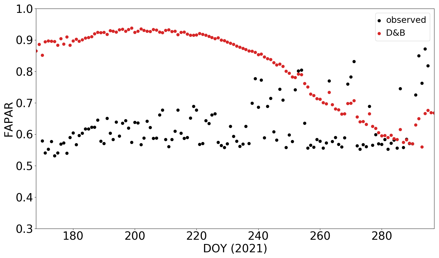
Figure 8 Observed (black) and simulated (red) FAPAR at Sodankylä between 19 June and 22 October 2021. Simulated FAPAR is for the evergreen conifer PFT only, in accordance with the vegetation within the field of view of the FAPAR sensor.

Extensive LAI sampling during summer 2022 from hemispherical photographs gives an average value of 1.37, and measurements using LI-COR LAI-2200 give an average value of 1.32. These agree rather well with a simulated annual-average LAI of 1.3 for the tree PFT; however, there is a pronounced seasonality of simulated LAI corresponding to the seasonality of FAPAR seen in Fig. 8, with significantly lower values for September (DOY 244 to 273: 1.37) than for mid-June to the end of August (from DOY 166 to 243: 2.96). The across-plot average at different dates from the hemispheric photographs show no such seasonality, with a June-to-August average (measured on DOYs 166, 192, 207, 212 and 217) of 1.39 vs. a September average of 1.34 (measured on DOYs 254 and 271).

5.2 Evaluation of SIF simulations

SIF measurements provide an opportunity to document the presence of photosynthetically active plant material and are therefore an interesting quantity for model validation. At the Sodankylä site, the observations started in spring 2021 as part of the LCC campaign activities. The measurement angle was adjusted in early June; therefore, we show comparisons to the simulations starting only from 3 June onwards.

Simulated SIF values are shown here (Figs. 9 to 11) with a multiplication factor of 10, i.e. with the scaling factor s_SIF in the SIF source term, Eq. (1), set to 10. While the prior value of s_SIF was 1, this change reflects the high uncertainty regarding the absolute magnitude of the measured SIF. Observations are shown for two methods of retrieving SIF from the actual measurements, namely Fraunhofer line discrimination and spectral fitting (see Sect. S3.5).

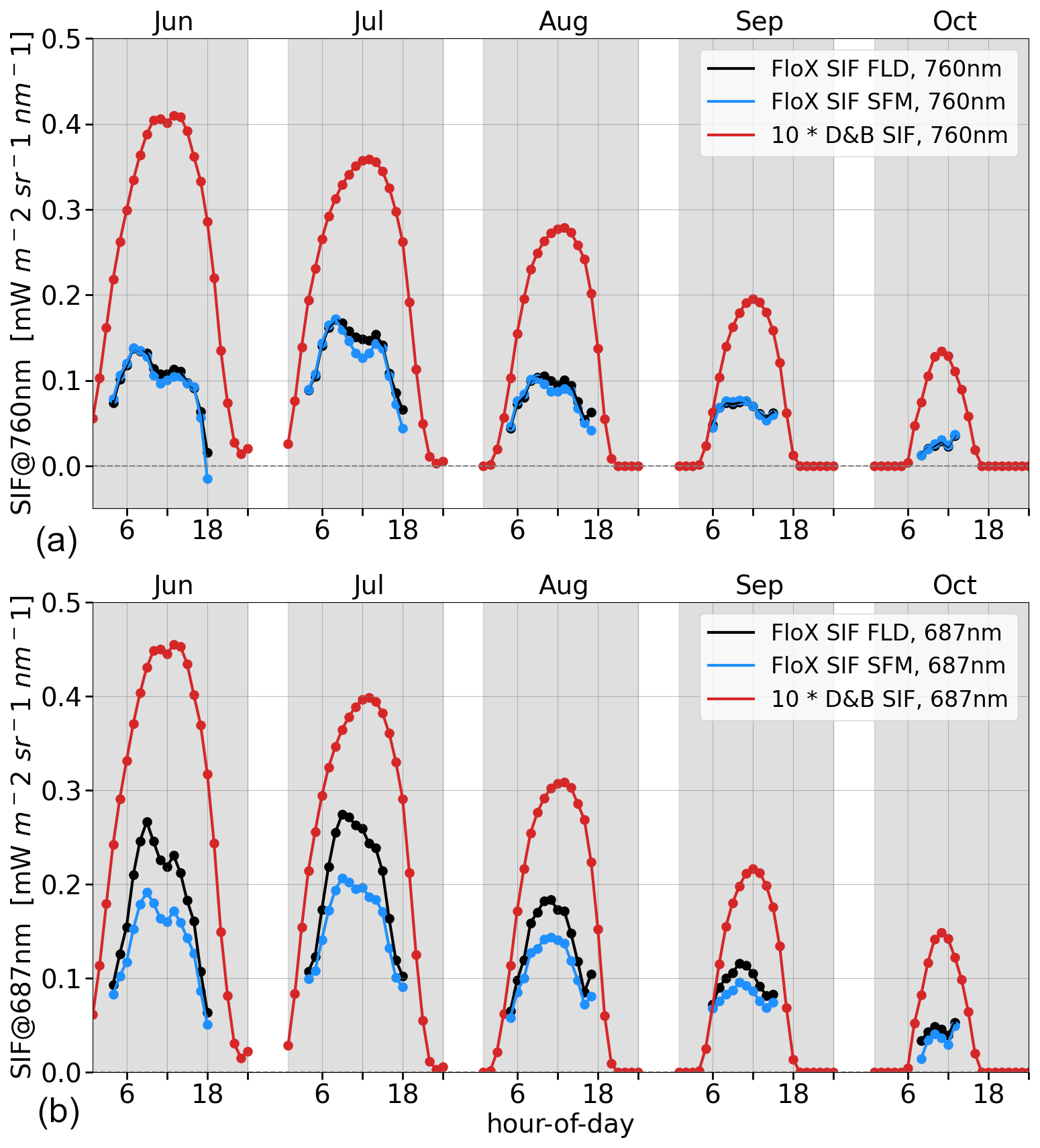
Figure 9 Average diurnal cycle by month of far-red (a) and red SIF (b) for pine forest (PFT 5) at Sodankylä for the months of June to October in 2021. D&B simulations (red) against measurements with the fluorescence box (FloX): retrievals made with the Fraunhofer line discrimination (black) and retrievals made with the spectral fitting method (blue).

The difference in magnitude between the modelled and observed SIF is likely due to the choice of prior parameters for the SIF model, taken from Gu et al. (2019), and the specific spectral conversion used (Eq. 2). Although it has not been done here, there is scope within D&B to adjust these parameters in the assimilation. This is achieved through calibration of the scaling factor s_SIF in the observation operator for SIF (Eq. 1). Given that the model with its prior parameter set can already track the seasonal and diurnal cycle of the observations reasonably well, we expect that SIF measurements will be able to provide constraints on processes that affect the temporal evolution of photosynthetic rates, such as leaf phenology, or timing of stomatal closure.

At the Sodankylä site, the simulations are able to track both the diurnal and seasonal cycles of the observations reasonably well (Fig. 9). However, there are indications of water stress in the measured diurnal cycles in June, July and August. These are shown as a dip in the far-red SIF during midday (Fig. 9a) and also for June in the red SIF (Fig. 9b). The decline in SIF is likely due to a midday depression of photosynthesis (Lin et al., 2024). The model reproduces this behaviour only for June and to a much lesser extent. Also, the model shows larger SIF signals for June compared to July but not the measurements. Since the midday depression is observed as a response to stomatal closure due to water stress, the comparison indicates that the model underestimates water stress at the boreal site. The simulations also show an earlier increase and later decrease during the day during the summer months. This may partly be attributed to retrieval problems for high sun zenith angles.

The measured far-red SIF (760 nm) of the trees at the Majadas de Tiétar site (PFT 3, Fig. 10a) shows a clear seasonal cycle of SIF peaking in July. For the red SIF (687 nm, Fig. 10b), there is no clear seasonal maximum. This is independent of the retrieval method. The model by contrast shows a clear peak in May. The diurnal cycle of SIF in the model peaks later, usually around 14:00 LT (local time) and extends further into the afternoon compared to the measurements, which peak around 11:00 to 12:00 LT (central vertical line).

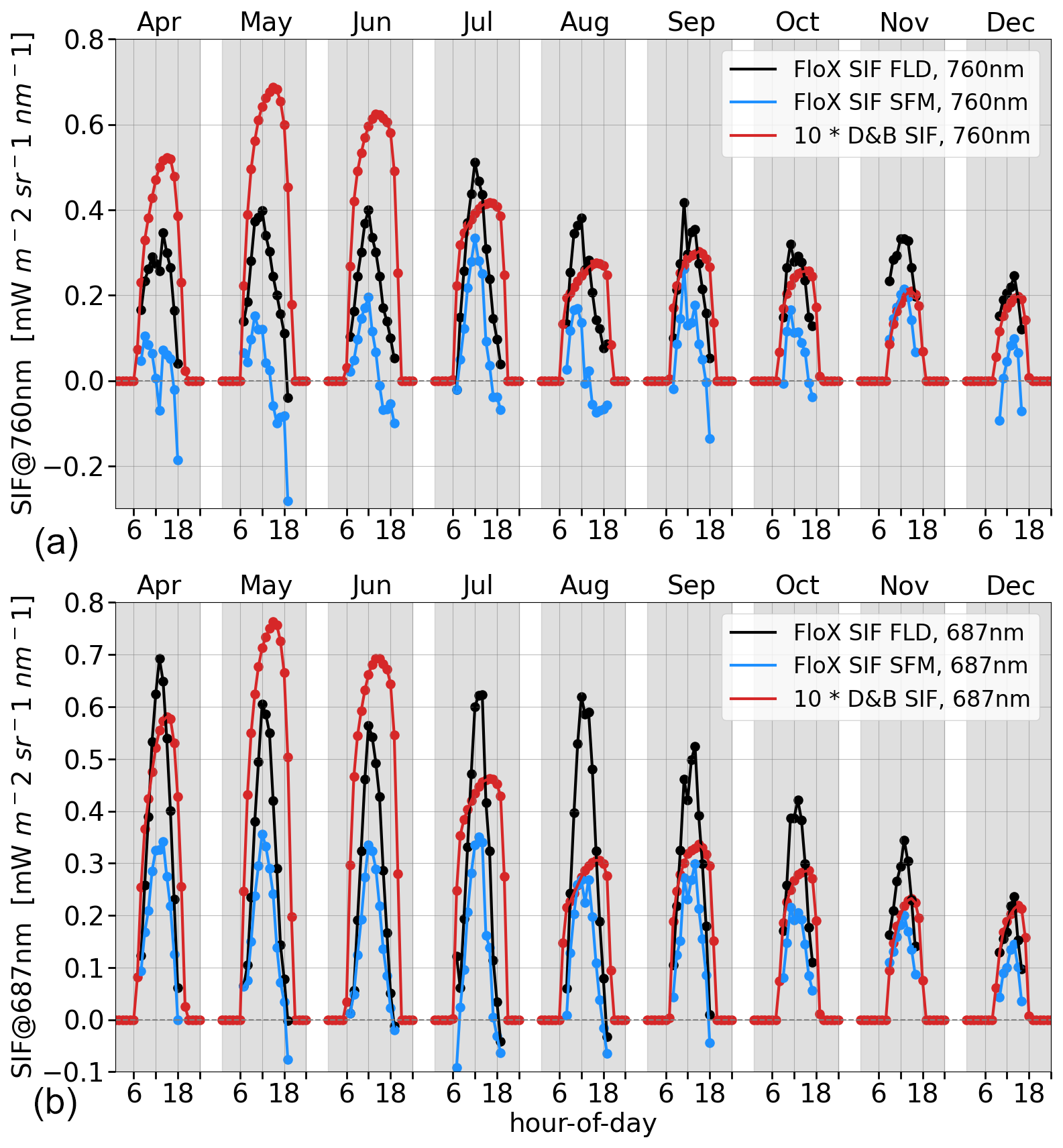
Figure 10 Average hourly diurnal cycle by month of SIF in the far-red (a) and red (b) for evergreen trees (PFT 3) at Majadas de Tiétar for the months of April to December in 2021. D&B simulations (red) against measurements: retrievals made with Fraunhofer line discrimination (black) and the spectral fitting method (blue).

By contrast, the SIF measurements for grass (PFT 9) show almost complete senescence of the grass during June and July when using the spectral fitting method, but there is some remaining activity when using Fraunhofer line discrimination of the red-spectrum signal (Fig. 11). For this combination (red SIF with Fraunhofer line discrimination), model simulations are in good agreement with the measurements, with a suitable scaling factor s_SIF in the SIF source term (Eq. 1). However, judging from the other spectral bands or retrieval methods, the results suggest that the model may underestimate the water stress of the grasses.

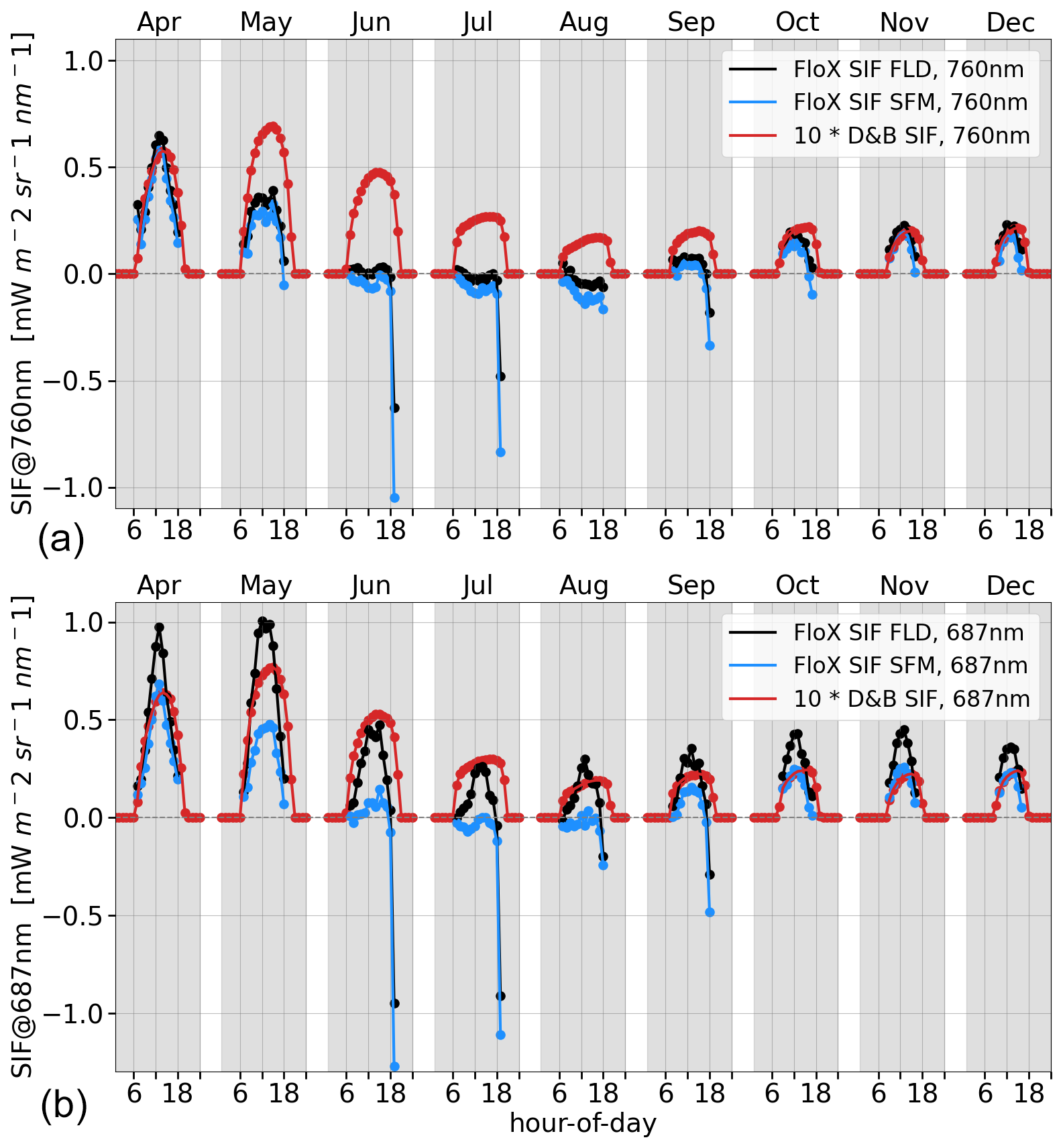
Figure 11 Average hourly diurnal cycle by month of SIF in the far-red (a) and red (b) for C₃ grass (PFT 9) at Majadas de Tiétar for the months of April to December in 2021. D&B simulations (red) against measurements: retrievals made with Fraunhofer line discrimination (black) and the spectral fitting method (blue).

5.3 Evaluation of VOD simulations

Figure 12 shows the comparison between observed and simulated L-VOD for the period after the first change in measurement geometry (for all three elevation angles) for the Sodankylä site. Observations only include the trees; therefore, simulated L-band VOD is for the tree PFT only. The temporal variations of the measurements are well captured by the simulation, in particular after the second change in viewing geometry after DOY 280.

Figure 12 L-band VOD from Elbara II over a pine stand (PFT 5) for different elevation angles compared to D&B simulated L-band VOD for PFT 5 only. Time axis starts on 18 September 2021 when the azimuth angle of the Elbara II instrument was changed for the first time.

The increase in biomass in the field of view through the first change in measurement geometry on 17 September (DOY 260) was estimated to be a factor of 3 (see Sect. S3.6). The revised field of view was also found to better represent typical conditions of the wider area, with the initial field of view capturing the signal from much sparser vegetation. To simulate L-VOD for the period before DOY 260, we therefore reduced assumed biomass entering the VOD observation operator (C_wd, C_fol in Eq. 4) to one-third of their default modelled values.

With this provision, the simulations match both the temporal variations and the magnitude of the locally measured L-VOD rather well (Fig. 13; see Sect. S3.6 for the default simulations). This includes the rise in spring, including a peak around DOY 60, and also temporal variations between DOYs 90 and 130. Only the period ca. DOYs 130 to 180 shows a systematic overestimate compared to measurements. A slow decline after DOY 220 is also reproduced by the model. We thus find a very satisfactory performance of the empirical L-VOD observation operator together with D&B.

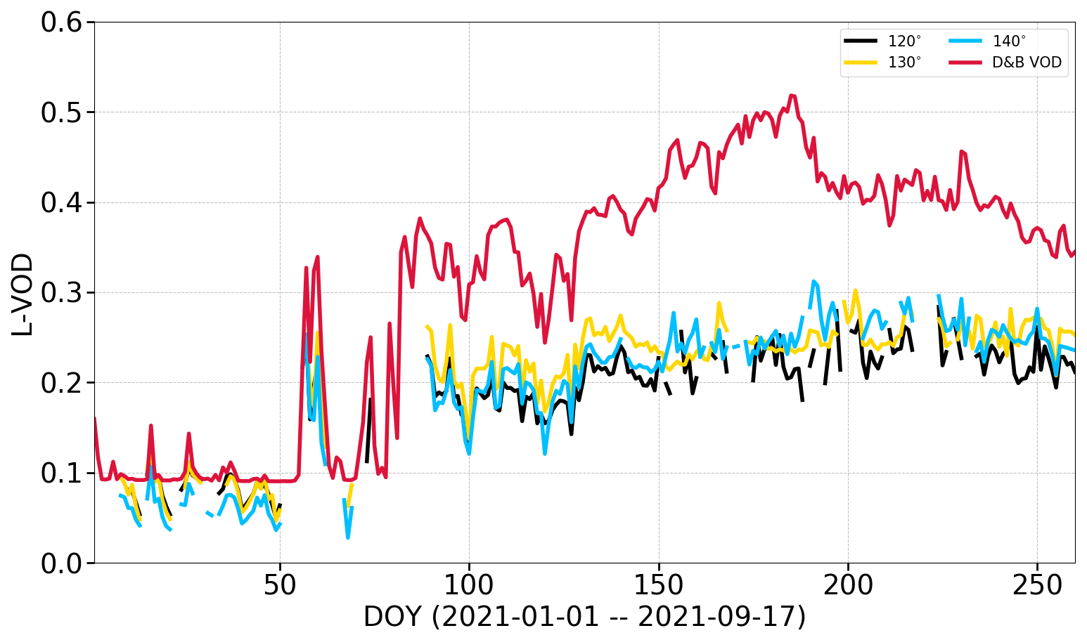
Figure 13 L-band VOD from Elbara II over a pine stand (PFT 5) for different elevation angles compared to D&B-simulated L-band VOD, for PFT 5 only, before first change in view geometry, with biomass reduced to $\mathrm{1}/\mathrm{3}$ of default simulated values.

5.4 Evaluation of surface soil moisture

Measured soil moisture at Sodankylä (Fig. 14) shows very similar temporal variations between different depths. The temporal variations of the D&B simulations are also similar, only that the overall magnitude differs, even though the magnitude of the shallowest measured depth (5 cm) is closest to the model. We point out that the depth of the surface layer in D&B is 4 cm. Both measurements and simulations also indicate significant interannual variability, with some years (e.g. 2019, 2020) exhibiting some pronounced summer drying, of which only some is captured by the measurements due to data gaps.

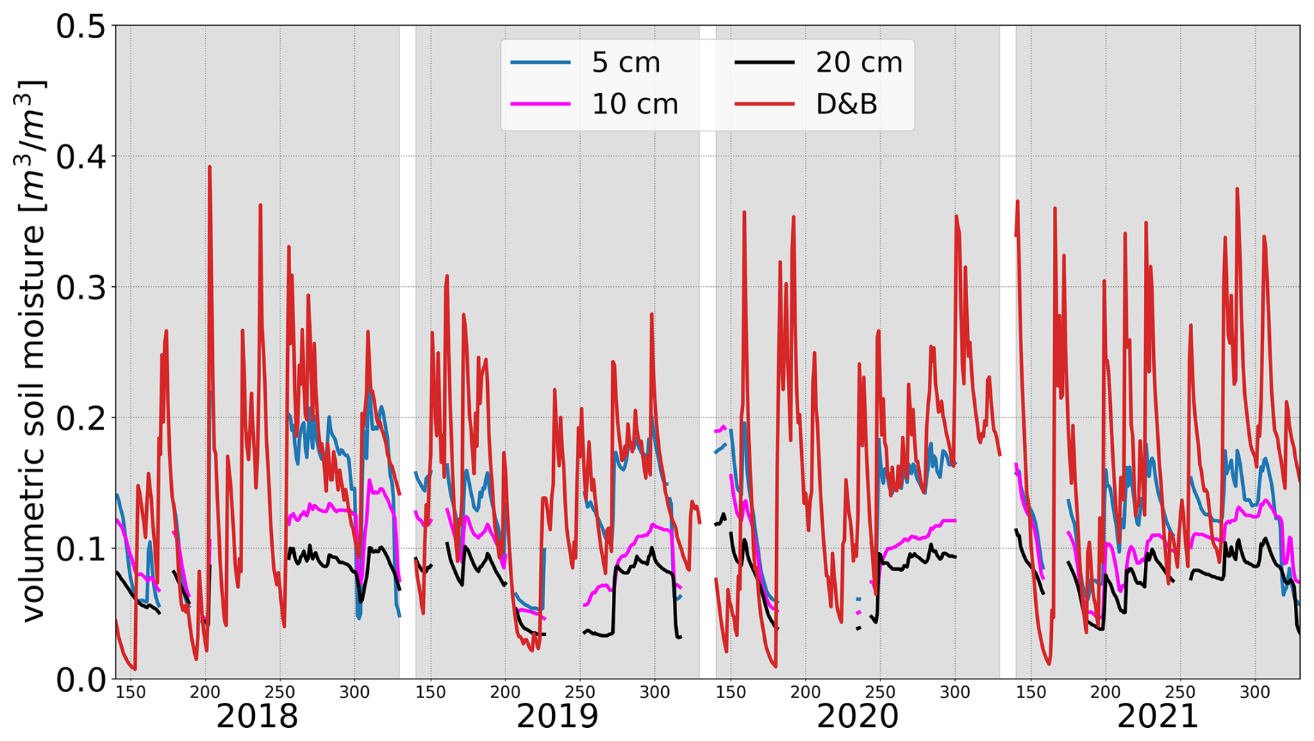
Figure 14 Daily in situ observed soil moisture at 5, 10 and 20 cm depth and simulated near-surface soil moisture, W_s, at Sodankylä for DOYs 140–330 in the years 2018–2021. Winter months not shown to avoid impact of frost on soil moisture sensors.

At Majadas de Tiétar, variations in soil moisture measured between different depths are again relatively small, showing that the exact depth for which these are simulated is of lesser importance (Fig. 15). In fact, the two depths closest to the surface (5 and 10 cm depth) show an almost identical temporal profile, including the magnitude of the maximum soil moisture depletion during the summer (July, August). The main characteristics of the observed seasonal cycle are also well reproduced by the D&B model. The timing of individual rain events can be traced in the measurements and is well reproduced by the simulations, including the lack of such events during the summer months. However, in the simulations, soil moisture decreases to near zero, whereas according to the measurements some soil moisture remains even at the peak of the summer.

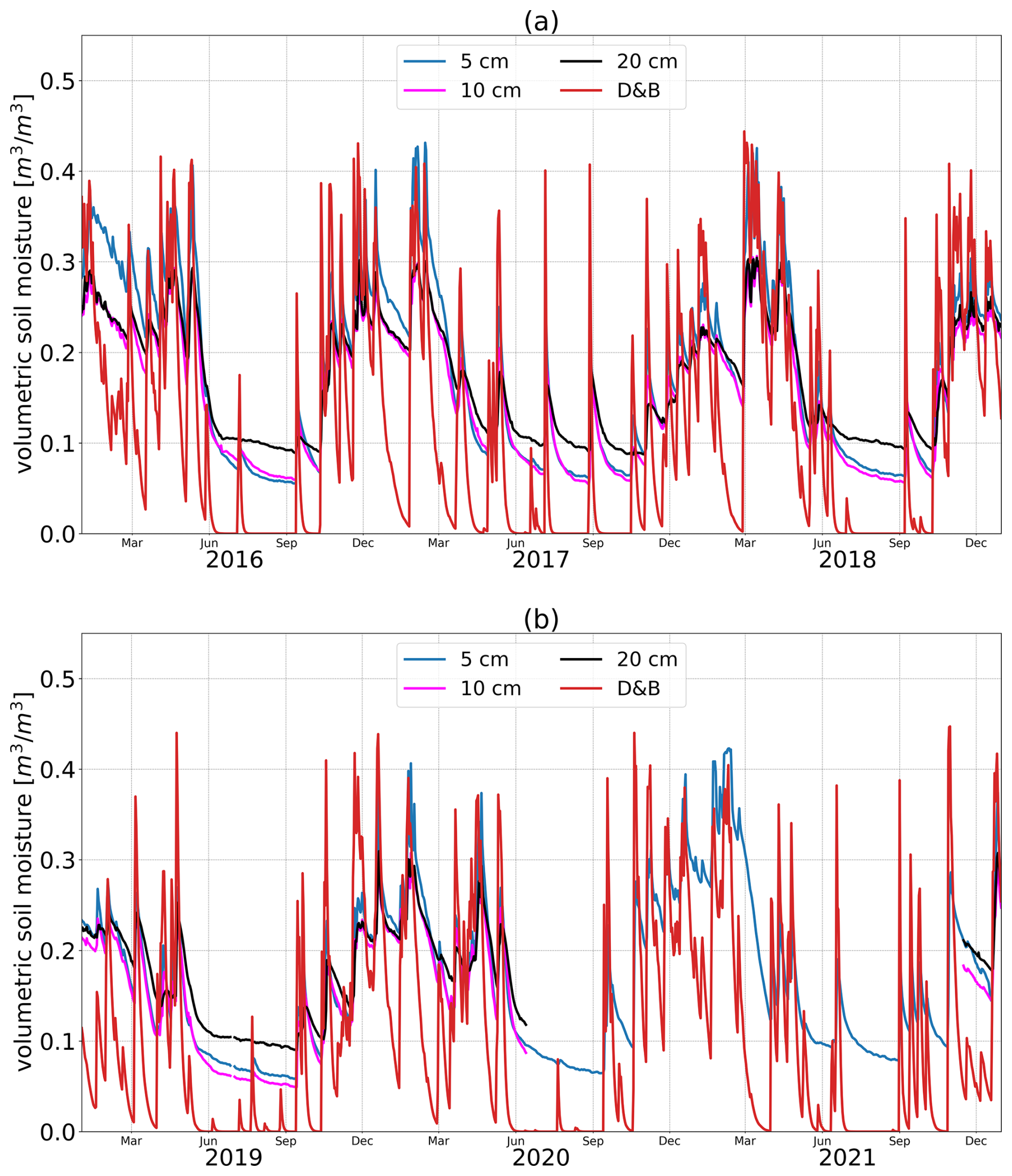
Figure 15 Daily in situ observed soil moisture at 5, 10 and 20 cm depth and simulated near-surface soil moisture, W_s, at Majadas de Tiétar for the years 2016–2018 (a) and 2019–2021 (b).

6 Discussion

6.1 Implications of study results

The comparison of the model simulations at the two sites against local data indicates that D&B does a reasonable job at representing energy and carbon fluxes between the atmosphere and terrestrial vegetation, albeit with the seasonal amplitude of the net carbon exchange overestimated at the boreal site. The comparison shows that carbon fluxes in particular are simulated reasonably well, with lesser agreement for energy fluxes but also significant imbalances between the measured energy fluxes and the net radiation available to the canopy; i.e. there is a significant deviation from energy closure. We conclude that there is a need for multi-stream data sources to be used for evaluating carbon and water flux models of terrestrial ecosystems, as opposed to relying chiefly on eddy covariance data.

The addition of dedicated observation operators led to further insights regarding model performance. In particular, local SIF measurements further revealed the power of those measurements to detect limitations on photosynthesis, such as water stress, beyond the capability of FAPAR measurements, despite remaining uncertainties regarding the absolute magnitude of the simulated SIF signal (see Fig. 9). We were able to identify a possible underestimate of soil water limitation of the Scots pine forest at Sodankylä during the summer, which may partly explain why the model overestimates GPP at this site.

At the Majadas de Tiétar temperate-savannah site, we clearly identified that the model underestimates latent heat flux during the summer months, while it also underestimated the site's overall photosynthetic uptake (GPP). This underestimation appears to be a result, in particular, of the model overestimating moisture limitations of the savannah ecosystems during the summer, possibly due to non-matching parameterisation of the stomatal model. This matched the insights provided by the SIF measurements that the trees of the ecosystem continue transpiring and photosynthesising across the summer without major limitations due to water stress. Surface soil moisture data also indicated too much soil drying during the summer months. Possibly, the model fails to represent the strongly heterogeneous soil texture at Majadas de Tiétar, with a sandy top and deeper clay soil, underestimating the soil water holding capacity of the deeper soil layers to which only the trees have access. These considerations demonstrate the added value of the dedicated observation operators for the evaluation of D&B at the local scale.

6.2 Potential for further applications

The process model in combination with its observation operators presented here has been designed to be used within a variational data assimilation framework, planned to be set up following the existing CCDAS (Rayner et al., 2005). This means that D&B will be complemented with tangent and adjoint versions, which efficiently provide derivative information for variational assimilation. The anticipated default setup in data assimilation mode is for combined calibration and initialisation, i.e. adjustment of parameters of the process model and its observation operators and of the initial state of the carbon pools. Assimilated data streams are planned to come chiefly from Earth observation sources. This setup will provide both capabilities for assimilating more data streams than previous studies (e.g. Scholze et al., 2019) while also including a full description of biomass pools as so far provided by other, more complex process models, e.g. LPJ-GUESS (Smith et al., 2001), albeit with lesser data assimilation capabilities.

In anticipation of such an application, we have in this contribution refrained from adjusting individual parameters by hand in order to improve the match to any of the validation data sets used in Sects. 4 and 5. However, we can already assess, to an initial degree, the potential of the system to obtain a superior fit to measurements by way of optimising its parameters. As an example, comparing measured and simulated surface soil moisture (Sect. 5.4) and taking into account the model's functional dependencies, we can infer that changing the assumed texture of the soil near its surface will immediately change the absolute magnitude of the simulated signal but have only a negligible impact (via soil evaporation) on its temporal course.

In particular, the good match between simulated and locally measured L-VOD, which includes details of most temporal variations, offers considerable opportunities for the assimilation of widely available satellite-derived L-VOD over larger regions.

6.3 Limitations

While the initial task to match and compare modelled and observed data streams was successfully demonstrated, the results of this study also point at the need to further investigate the representation of the seasonal cycle of LAI in northern evergreen conifer forests and shrubs. Earth observation products for the boreal region show seasonality in LAI that is not consistent with ecological expectation and FAPAR data. The phenology scheme of D&B has the flexibility to simulate vegetation with a small amount of seasonal variation in LAI if corresponding information is provided for the prior calibration of the parameters in the phenology scheme. Such information could come from field observations of LAI time series in boreal regions or improved satellite products.

Another issue that occurred is that the scaling factor s_SIF in the SIF source term (Eq. 1) is highly uncertain. In a data assimilation mode, it would be included (possibly in a PFT-specific form) in the list of parameters to be adjusted. This would effectively allow for scaling the simulated SIF time series shown in Figs. 9, 10 and 11. Similarly, the parameters in the empirical observation operator for VOD would also be included in the set of parameters to be adjusted in assimilation mode. We also note that many of the model's parameters are not very well constrained and could therefore change substantially. For example, an adjustment of the turnover times for the litter and soil organic matter pools will change heterotrophic respiration, and, according to Eq. (S153), the fit to simulated TER shown in Figs. 3 and 6. This could happen in the framework of either a local-scale assimilation of eddy flux measurements as used here for evaluation or on a regional or global scale with the assimilation of atmospheric CO₂ data, including those from space-based remote sensing (Buchwitz et al., 2017).

A further limitation we found is that the model overestimates soil water limitation at the savannah site. This may be linked to the parameterisation of soil hydrological properties or to the parameterisation of rooting depth and root penetration of the soil, both of which warrant further investigation. We also find that the model may overestimate soil evaporation for very dry soils.

A principal advantage of the process-based modelling approach presented here is that the system can be used to identify, better investigate and quantify specific processes – a fundamental and often decisive advantage over machine learning or complex statistical modelling systems (Thessen, 2016; Lary et al., 2018). The advantage translates into a principal limitation in that if a given process contributes to the measured signal, it has to be represented. Otherwise, missing process representation can lead to misleading parameter choices that use processes included within the system to compensate for the missing process – also known as “matching observations for the wrong reasons”. Therefore, process modelling requires significant expert knowledge on ecosystem functioning as well as experience with or direct contact to experimental teams, compared to statistical interference methods, including machine learning – which by definition can never be right for the wrong reasons, as they are used essentially as black boxes. The potential advantage of D&B coupled to multiple observation operators is that it allows for model testing via multiple data streams, thus providing a more comprehensive model evaluation which makes it less likely that the model matches observations while misrepresenting important processes.

6.4 Outlook

In this study, we have shown the value of the four data streams (FAPAR, SIF, VOD and surface soil moisture), as opposed to the intrinsically local measurements used for the initial evaluation, which lies in their availability over large spatial scales. Therefore, such data streams derived from Earth observation sources will make it possible to evaluate the model across larger regional scales. The immediate next step would therefore be to evaluate D&B with regional rather than local observations and see if in such a setup the noted model–observation differences are reduced. The advantage of regional comparisons is that substantial uncertainties arising from small-scale conditions are averaged out, and the scale of comparison may by more appropriate for a typical application of the model.

At such a regional scale, it will further be possible to assimilate those data streams using the principal setup described above. Here, it will be possible to adjust parameters either spatially grouped by PFT, following CCDAS (Kaminski et al., 2013), or independently at each pixel, following DALEC (Quaife et al., 2007). A further approach that has not yet been tested would be a combination of the two, where parameters are adjusted at every grid cell independently but with a partial constraint on parameter values assuming that those values co-vary depending on closeness of geographical location, altitude, land use, PFT or soil type.

A significant advantage of such a data assimilation system will be the possibility to investigate if the process model is capable of matching the observations not only for a specific parameter set but also within reasonable bounds of the entire model parameter space. Only if that is not possible can we rigorously conclude that the remaining model–observation mismatch is caused by a missing or unsuitable process representation. We consider such investigations the next logical step of development of the D&B modelling system, besides any inclusion of further Earth observation data streams. The further goal would then be to apply it to the task of routinely producing data products on carbon and energy fluxes.