A Bayesian method for predicting background radiation at environmental monitoring stations in local-scale networks

Detector networks that measure environmental radiation serve as radiological surveillance and early warning networks in many countries across Europe and beyond. Their goal is to detect anomalous radioactive signatures that indicate the release of radionuclides into the environment. Often, the background ambient dose equivalent rate ${\dot{H}}^{*}\left(\mathrm{10}\right)$ is predicted using meteorological information. However, in dense detector networks, the correlation between different detectors is expected to contain markedly more information. In this work, we investigate how the joint observations by neighbouring detectors can be leveraged to predict the background ${\dot{H}}^{*}\left(\mathrm{10}\right)$. Treating it as a stochastic vector, we show that its distribution can be approximated as multivariate normal. We reframe the question of background prediction as a Bayesian inference problem including priors and likelihood. Finally, we show that the conditional distribution can be used to make predictions. To perform the inferences we use PyMC. All inferences are performed using real data for the nuclear sites in Doel and Mol, Belgium. We validate our calibrated model on previously unseen data. Application of the model to a case with known anomalous behaviour – observations during the operation of Belgian Reactor 1 (BR1) in Mol – highlights the relevance of our method for anomaly detection and quantification.

1 Introduction

Networks that measure environmental radiation are operational in countries across Europe and beyond. Such networks monitor the environment for aberrant radioactivity that could, for example, indicate the anomalous release of radionuclides from a nuclear facility. Within Europe, observations of national networks are collected on the EUropean Radiological Data Exchange Platform, EURDEP (European Commission, 2024; Sangiorgi et al., 2020), including those of the Belgian radiological surveillance network and early warning system TELERAD (Sonck et al., 2010). Some stations come equipped with gamma-spectrometric capabilities that allow for observing the contributing gamma energies, which can be used to tease out the responsible radionuclides. More often, however, stations use Geiger–Müller tubes to measure the ambient gamma dose equivalent rate (nSv h⁻¹), denoted as ${\dot{H}}^{*}\left(\mathrm{10}\right)$. A difficulty with detecting and quantifying anomalies based on ${\dot{H}}^{*}\left(\mathrm{10}\right)$ is that gamma radiation also occurs naturally and varies as a function of time. To distinguish anomalous from normal behaviour using these detectors, therefore, one must establish what normal really means.

Under normal conditions, terrestrial radiation contributes significantly to ${\dot{H}}^{*}\left(\mathrm{10}\right)$. Potassium-40 is abundant in nature, as are the radionuclides in the uranium and thorium decay chains. When those decay chains reach radon (radon-222) and thoron (radon-220), both noble gases, exhalation occurs from the soil to the atmosphere. Radon is usually dominant over thoron due to its much longer decay time (3.8 d versus 56 s). Only radon is long-lived enough for it to be able to be transported over considerable distances through air. During precipitation events, radon daughters (lead-214 and bismuth-214) are deposited on the ground again via wet scavenging (Sportisse, 2007), which accounts for increased ${\dot{H}}^{*}\left(\mathrm{10}\right)$ (Mercier et al., 2009; Livesay et al., 2014). Besides natural radionuclides, anthropogenic contributions also exist. Caesium-137 fallout from the atmospheric nuclear weapons tests of the 1950s and early 1960s, with some as late as 1980 (Bergan, 2002), and of the Chornobyl accident in 1986 still contributes to ${\dot{H}}^{*}\left(\mathrm{10}\right)$ due to its long half-life of 30.8 years according to a complex spatial pattern (European Commission et al., 1998). Other anthropogenic sources (e.g. medical or industrial) also contribute to the inventory of environmental radionuclides (Maurer et al., 2018) although these will usually be too small to affect ${\dot{H}}^{*}\left(\mathrm{10}\right)$. Finally, cosmic radiation, at ground level mainly muons, contributes significantly to the background ${\dot{H}}^{*}\left(\mathrm{10}\right)$. We refer to the sum of these processes as background radiation. In the rest of this work, we will exclusively refer to background radiation to mean these normally occurring processes and anomalous radiation to be everything other than these normally occurring processes.

Our ability to identify and quantify anomalous radiation hinges on our ability to predict the behaviour of the background. This is relevant not only for the aforementioned detector networks, but also for mobile measurement campaigns which were used, for example, in the aftermath of the Fukushima nuclear accident (Querfeld et al., 2020; Nomura et al., 2015). Even without factoring in unknown sources, the background is a complex function of space and time governed by, for example, geological properties of the soil, land use, and (space) weather. The multifaceted nature of environmental radioactivity precludes first-principles modelling, which makes predicting the background a difficult problem. In lieu of comprehensive first-principles approaches, a rich variety of data-driven solutions exist. Various machine learning approaches have been investigated to forecast background radiation based on dose rate time series (Arahmane et al., 2024; Breitkreutz et al., 2023). Recently, long short-term memory networks (LSTMs) have shown promise in predicting background radiation based on meteorological parameters like temperature, humidity, and wind speed (Liu and Sullivan, 2019; Breitkreutz et al., 2023). When the goal is spatial interpolation rather than temporal prediction, kriging methods have been successfully employed to construct, for example, national maps based on (airborne) radiation measurements (Chernyavskiy et al., 2016; Folly et al., 2021). Bayesian approaches to background estimation exist predominantly in the context of source localisation, using either spectral data (Howarth et al., 2022) or gross count rates (Michaud et al., 2021; Brennan et al., 2005). Often, such approaches do not resolve full posterior distributions, instead relying on more computationally efficient maximum likelihood estimation (MLE). MLE approaches have also been used to discriminate between spatial background inhomogeneity in the built environment and temporal inhomogeneity due to precipitation (Liu et al., 2018).

In the current work, we present a Bayesian inference framework for the estimation of the background ambient dose equivalent rate observed in densely packed local detector networks. We assume that the processes that drive changes in the background occur at a scale that is larger than the typical scale of the local networks under consideration, and we model the response to such an external driver by looking at the effect that it has on all detectors. What sets our work apart from other work is the fact that we allow for correlations between the different detectors in the network, so the external driver does not necessarily affect all detectors equally. The Bayesian approaches mentioned in the previous paragraph all assume that the different observations are independent so that the likelihood given a large set of data simply becomes the product of the likelihoods of the individual data points. Doing so simplifies sampling the posterior significantly. In allowing for correlations, we add significantly to the dimensionality of the Bayesian inference problem – because it requires the estimation of a correlation matrix between the detectors in the network – but we get a more truthful parameterisation. Using this model, we can estimate independent means for each detector, the variance that is intrinsic to each detector due to a combination of counting statistics and measurement noise, and the collective response of the network to meteorological drivers.

The rest of this paper is structured as follows. In Sect. 2, the data and methods are described. Starting from an introduction of the TELERAD detector network, specifically the sub-networks around two nuclear facilities in Belgium, we derive a Bayesian inference problem and describe how to solve it. Additionally, we describe how the Bayesian inference problem can be extended to also allow for predictive modelling. In Sect. 3, we describe calibration and verification of our Bayesian model using various subsets of TELERAD data. In Sect. 4, we show how calibrated models can be leveraged to make predictions. Finally, in Sect. 5, we study a case that is relevant in an operational context. Using the detectors from one nuclear site (Doel) to predict the dose rate at detectors from another nuclear site (Mol) while an atmospheric release is ongoing at the latter shows how our work can be useful in anomaly detection.

2 Data and methods

2.1 The TELERAD detector network

We first present the detector network that we try to model. TELERAD, the radiological surveillance network and early warning system in Belgium (Sonck et al., 2010), measures the extent of radiological contamination both in air and soil and in water using a variety of techniques. For atmospheric measurements using gamma dosimetry, three sub-networks exist. The Immission Monitor for National area (IMN) covers the entire Belgian territory, the Immission Monitor for Agglomeration area (IMA) covers only those populated areas within several kilometres of nuclear facilities, and the Immission Monitor for Ring area (IMR) covers the immediate vicinity of nuclear facilities. Such a network is not unique to Belgium, as described in the Introduction (see Sect. 1), but the Belgian network is among the densest networks in the world. Hourly values for the IMN and IMA, dating back many years, are also publicly available on a Belgian national platform (Federal Agency for Nuclear Control, 2024) similar to EURDEP (European Commission, 2024).

We use data from IMR stations at two nuclear sites: the Belgian Nuclear Research Centre (SCK CEN) in Mol and the nuclear power plant (NPP) in Doel. The layouts of the detector networks at Doel and Mol, as well as their locations in Belgium, are shown in Fig. 1. Characteristic of the Doel site are the river Scheldt bordering it to the east and the flat farmland bordering it in other directions. Eighteen IMR stations, D01 through D18, sit along its perimeter. Characteristic of the Mol site is the largely forested area. IMR detectors are set up more complicatedly than in Doel owing to the presence of several nuclear facilities. Stations M07 through M13 surround Belgian Reactor 1 (BR1); detectors M01 through M04, M14, and M15 surround Belgian Reactor 2 (BR2); and stations M05, M06, and M16 are south of Belgian Reactor 3 (BR3). BR1 and BR2 are still operational today; BR3 has been decommissioned and is being dismantled. Of these detectors, we exclude M12 from further analysis because of several corrupted entries in the database.

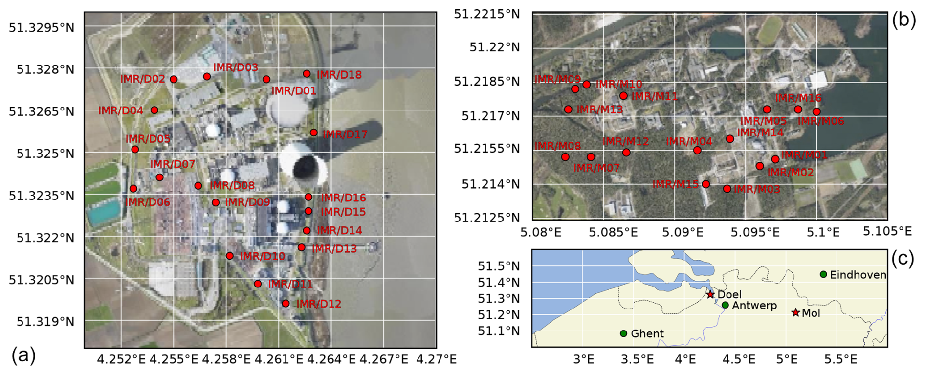
Figure 1 Maps of the TELERAD stations at the (a) Doel and (b) Mol sites. (c) The locations of Doel and Mol in Belgium. The Cartopy package (Elson et al., 2024) was used to generate the maps using aerial footage from Agentschap Digitaal Vlaanderen (2016) and geographic vector data from Natural Earth (2024).

In this work, we analyse four different combinations of IMR stations. Case BR1 includes those IMR stations that form a ring around BR1. Case MOL includes all IMR stations at SCK CEN. Case DOEL includes all IMR stations at Doel NPP. Finally, case DOEL–BR1 includes a subset of IMR stations at Doel NPP and the IMR station included in case BR1. Details are listed in Table 1.

Table 1 The four different combinations of IMR stations that are examined in this study.

All IMR stations measure the 10 min averaged ambient dose equivalent rate ${\dot{H}}^{*}\left(\mathrm{10}\right)$, which is measured in nanosieverts per hour (nSv h⁻¹). According to the definition by the ICRP (2020), “the dose H^*(d), at a point in a radiation field, is the dose equivalent that would be produced by the corresponding expanded and aligned field in the ICRU sphere at a depth, d, on the radius opposing the direction of the aligned field”. The ambient dose equivalent rate is the time derivative of the ambient dose equivalent evaluated at a depth of d=10 mm. Many IMR stations also have gamma-spectrometric capabilities, and at low dose rates the ambient dose rate is actually calculated as the accumulated spectrum rather than measured using the Geiger–Müller detector. In this work, we only look at dose rate data. Data from three periods are used: 6 August through 13 August 2022, 30 August through 1 September 2022, and 10 through 12 September 2022. Selection of these data was subject to BR1 non-operation and no precipitation. BR1 is not operated for a while during July–August, and we found the period from 6 through 13 August to also be without precipitation. The other two periods were chosen to be several weeks later than this initial period to check the temporal stability of the calibration, one requiring reactor non-operation (30 August through 1 September) and the other requiring reactor operation (10 through 12 September). Data for all three periods are available on Zenodo (Frankemölle et al., 2024a).

To supplement the data, we use source monitoring data for BR1 and precipitation data. The former are necessary because BR1 is an air-cooled reactor, the operation of which causes a noticeable artificial increase in on-site ${\dot{H}}^{*}\left(\mathrm{10}\right)$. This is not the case for the other facilities. Source term data are obtained from an in-stack monitor (Frankemölle et al., 2022b). Precipitation data are taken from nearby precipitation monitoring stations in Retie, approximately 2 km northwest of SCK CEN, and Melsele, approximately 10 km south of Doel NPP (Vlaamse Milieumaatschappij, 2023).

2.2 Modelling background radiation using Bayesian inference

To model measurements by the TELERAD sub-networks, we introduce a stochastic representation in Sect. 2.2.1 that we use to formulate a Bayesian inference problem in Sect. 2.2.2. In Sect. 2.2.3, we introduce the posterior predictive distribution to validate our Bayesian model.

2.2.1 Background radiation as a continuous stochastic vector

Consider the ambient dose equivalent (nSv) accumulated over a period T (equal to 10 min in the current study) as measured in our network:

$$\begin{array}{}\text{(1)}& \mathit{M}=\mathit{H}+\mathit{E},\end{array}$$

with $\mathit{M}=[M_{\mathrm{1}},\mathrm{\dots },M_k{]}^{\top }$ denoting the measurements reported in each sensor ($\mathrm{1},\mathrm{\dots },k$), $\mathit{H}=[H_{\mathrm{1}},\mathrm{\dots },H_k{]}^{\top }$ the real accumulated ambient dose equivalent in each sensor, and $\mathit{E}=[E_{\mathrm{1}},\mathrm{\dots },E_k{]}^{\top }$ the sensor measurement errors. We note that, typically, a dose rate is reported that corresponds to $\mathit{M}/T$ (nSv h⁻¹).

We represent the measured dose as a continuous stochastic (random) vector, which is driven by the real ambient dose equivalent, and the instrument error, both of which are stochastic processes themselves. We discuss the parameterisation of their distributions, which eventually leads to the parameterisation of the distribution of M.

Firstly, E represents the measurement noise. We can safely assume that errors are statistically independent between sensors. We further make the stronger assumption that the errors are normally distributed with zero mean, so $\mathit{E}\sim {\mathcal{N}}_k\left(\mathbf{0},{\mathbf{\Sigma }}_{\mathit{E}}\right)$ with Σ_E=diag [σ_E]I diag [σ_E], where ${\mathit{\sigma }}_{\mathit{E}}=[{\mathit{\sigma }}_{E,\mathrm{1}},\mathrm{\dots },{\mathit{\sigma }}_{E,k}{]}^{\top }$ denotes the standard deviations of the different sensor errors, which we infer in the Bayesian framework later. We note that the assumption of zero bias makes sense if instruments are properly calibrated, but validation of the Bayesian framework itself can also point to inconsistencies between sensor data which could point to the need for recalibration.

Secondly, we consider the real dose H. It is the accumulation of photons arising from the decay of a range of radionuclides that are present in the background around the sensor network. This is a process that is driven not only by the weather and other environmental phenomena, but also by the counting error resulting from the relatively low number of photons that hit the sensor. The latter can be approximated by a Gaussian distribution, but the former is much less trivial to describe. For lack of any detailed information on this distribution and to arrive at an elegant overall framework, we also presume the radionuclides' distribution to be Gaussian, but unlike E, we expect a large spatial correlation over the sensor network (although some aspects, such as the counting error or small-scale terrain effects, will not be correlated between sensors). With some further assumptions about the variabilities in both processes, we arrive at a Gaussian process for H as well, so $\mathit{H}\sim {\mathcal{N}}_k\left(\mathit{\mu },{\mathbf{\Sigma }}_{\mathit{H}}\right)$, and consequently,

$$\begin{array}{}\text{(2)}& \mathit{M}\sim {\mathcal{N}}_k\left(\mathit{\mu },{\mathbf{\Sigma }}_{\mathit{H}}+{\mathbf{\Sigma }}_{\mathit{E}}\right).\end{array}$$

At this point, we do not know the covariance matrices Σ_H and Σ_E – in Sect. 2.2.2 we use Bayesian inference to train possible distributions of their elements. We have

$$\begin{array}{}\text{(3)}& \begin{array}{rl}{\mathrm{\Sigma }}_{lm}& ={\mathrm{\Sigma }}_{\mathit{H},lm}+{\mathrm{\Sigma }}_{\mathit{E},lm}\\ & =\left\{\begin{array}{ll}{\mathit{\sigma }}_l^{\mathrm{2}}\triangleq {\mathit{\sigma }}_{\mathit{H},l}^{\mathrm{2}}+{\mathit{\sigma }}_{\mathit{E},l}^{\mathrm{2}}& \text{if}l=m,\\ {\mathit{\sigma }}_l{\mathit{\sigma }}_m{R}_{lm}& \text{otherwise},\end{array}\right.\end{array}\end{array}$$

where R with elements R_lm is the correlation matrix that we introduce here for later use. Thus, defining the diagonal matrix S=diag [σ] (with elements σ_l on the diagonal), we can also express Σ=SRS (Barnard et al., 2000).

Given k sensors and since R is symmetric, we have $\mathrm{3}k+k(k-\mathrm{1})/\mathrm{2}$ unknowns (in μ, Σ_E, Σ_H, and R), which we will train using Bayesian inference and a large dataset of measurements. However, given only measurements M and no additional information on the measurement errors, it is impossible to obtain separate information on σ_H and σ_E. Only σ can be determined, so in fact $\mathrm{2}k+k(k-\mathrm{1})/\mathrm{2}$ unknowns remain.

2.2.2 Training the mean vector and covariance matrix using Bayesian inference

Given a dataset $\mathcal{M}=\left[{\mathit{M}}_{\mathrm{1}},\mathrm{\dots },{\mathit{M}}_N\right]$, with 𝓜 an N×k matrix of measurements by the entire network of k detectors described in Sect. 2.1 at N different points in time, and given the stochastic variables of interest described in Sect. 2.2.1, we can write down Bayes's theorem (see Appendix A) for the posterior distribution $f(\mathit{\mu },\mathbf{S},\mathbf{R}|\mathcal{M})$. In terms of the likelihood $f\left(\mathcal{M}\right|\mathit{\mu },\mathbf{S},\mathbf{R})$, the prior $f(\mathit{\mu },\mathbf{S},\mathbf{R})$, and the evidence f(𝓜), this posterior is given as

$$\begin{array}{}\text{(4)}& f(\mathit{\mu },\mathbf{S},\mathbf{R}|\mathcal{M})={\displaystyle \frac{f\left(\mathcal{M}\right|\mathit{\mu },\mathbf{S},\mathbf{R}\left)f\right(\mathit{\mu },\mathbf{S},\mathbf{R})}{f\left(\mathcal{M}\right)}}.\end{array}$$

Strictly speaking, subscripts are required to indicate that Eq. (4) involves four different distributions. Instead, we denote all four distribution functions – of the posterior, likelihood, prior, and evidence – as f to avoid cluttering the equations. Their varying arguments are, after all, sufficient to tell them apart.

Here, we define the right-hand side of Eq. (4). The likelihood follows straightforwardly from Eqs. (2) and (3) as

$$\begin{array}{}\text{(5)}& \begin{array}{rl}f\left(\mathcal{M}\right|\mathit{\mu },\mathbf{S},\mathbf{R})& ={\displaystyle \frac{\mathrm{1}}{(\mathrm{2}\mathit{\pi }{)}^{k/\mathrm{2}}{\left|\mathbf{\Sigma }\right|}^{\mathrm{1}/\mathrm{2}}}}\\ & \times \prod _{i=\mathrm{1}}^N\exp \left[-{\displaystyle \frac{\mathrm{1}}{\mathrm{2}}}{\left({\mathit{M}}_i-\mathit{\mu }\right)}^{\top }{\mathbf{\Sigma }}^{-\mathrm{1}}\left({\mathit{M}}_i-\mathit{\mu }\right)\right],\end{array}\end{array}$$

where Σ=SRS with |Σ| being its determinant and Σ⁻¹ its inverse. While Eq. (5) implies M_i and M_j are independent of each other for i≠j, we should be careful not to take that at face value. Rather, this is a consequence of using the marginal distribution of some unknown higher-dimensional distribution that includes time. Since we are not interested in time, we marginalise the distribution; i.e. we “integrate out” the time. This is allowed even in the extreme case that E=0 and H is perfectly correlated in time. Marginalisation relates to drawing random samples from the time series, and so the only assumption that we actually make is that the time series is sufficiently long for it to cover the realisations of M.

The likelihood can be evaluated for any combination of μ, S, and R to determine how likely the observations 𝓜 are given that combination. This difference is particularly important when considering the evidence. For given observations 𝓜, the evidence f(𝓜) is just a number that normalises the posterior. Since we are only interested in the shape of the posterior rather than exact values, we can safely neglect it.

Finally, we consider the priors. The joint prior distribution $f(\mathit{\mu },\mathbf{S},\mathbf{R})$ can be simplified by assuming independence between μ, S, and R; i.e.

$$\begin{array}{}\text{(6)}& f(\mathit{\mu },\mathbf{S},\mathbf{R})=f\left(\mathit{\mu }\right)f\left(\mathbf{S}\right)f\left(\mathbf{R}\right).\end{array}$$

For f(μ), we choose a weakly informative prior by following the principle of maximum entropy, which yields the least informative priors given certain bounds on the support and statistical moments (Park and Bera, 2009). We know that μ is always equal to or larger than zero. Furthermore, we expect it to be centred on the time-averaged background level. The least informative prior with support [0, ∞) and a given mean is the exponential distribution

$$\begin{array}{}\text{(7)}& f\left(\mathit{\mu }\right)=\prod _{l=\mathrm{1}}^{k}f\left({\mathit{\mu }}_l\right),\end{array}$$

where $f\left(x\right)={\mathit{\lambda }}_l\exp [-{\mathit{\lambda }}_{l}x]$ and $\frac{\mathrm{1}}{{\mathit{\lambda }}_l}=\frac{\mathrm{1}}{N}{\sum }_{i=\mathrm{1}}^N{M}_{li}$.

For f(S), we choose the half-normal distribution (Gelman, 2006)

$$\begin{array}{}\text{(8)}& f\left(\mathbf{S}\right)=\prod _{l=\mathrm{1}}^{k}f\left(S_l\right),\end{array}$$

where $f\left(x\right)=\frac{\mathrm{1}}{{\mathit{\sigma }}_x}\sqrt{\frac{\mathrm{2}}{\mathit{\pi }}}\exp [-\frac{x^{\mathrm{2}}}{\mathrm{2}{\mathit{\sigma }}_x^{\mathrm{2}}}]$ for x≥0.

Finally, we formulate f(R). This is not trivial because not every combination of factors R_lm yields a matrix that is symmetric and positive semi-definite. To this end, we employ the LKJ correlation distribution (Lewandowski et al., 2009) over all possible correlation matrices. The advantage of the LKJ distribution is that it can be used as a prior for the correlation matrix R, allowing us to give a separate prior for the diagonalised scale vector S, as opposed to, for example, the inverse-Wishart distribution, which can only be used as a prior for the full covariance matrix (Gelman et al., 2013). We need the LKJ distribution, in effect, to work with the decomposition Σ=SRS (Barnard et al., 2000) that was introduced in Sect. 2.2.1. To be complete, here we reproduce from Lewandowski et al. (2009) the LKJ distribution function as

$$\begin{array}{}\text{(9)}& f\left(\mathbf{R}\right)=c_k{\left|\mathbf{R}\right|}^{\mathit{\eta }-\mathrm{1}},\end{array}$$

with |R| being the determinant of the k×k correlation matrix R; η being the sole shape parameter of the distribution; and c_k being the normalising constant, which only depends on the dimensionality k, as

$$\begin{array}{}\text{(10)}& \begin{array}{rl}{c}_k& ={\mathrm{2}}^{{\sum }_{l=\mathrm{1}}^{k-\mathrm{1}}\left(\mathrm{2}\mathit{\eta }-\mathrm{2}+k-l\right)\left(k-l\right)}\\ & \times \prod _{l=\mathrm{1}}^{k-\mathrm{1}}{\left[B\left(\mathit{\eta }+{\displaystyle \frac{\mathrm{1}}{\mathrm{2}}}\left(k-l-\mathrm{1}\right),\mathit{\eta }+{\displaystyle \frac{\mathrm{1}}{\mathrm{2}}}\left(k-l-\mathrm{1}\right)\right)\right]}^{k-l}.\end{array}\end{array}$$

Here B is the beta function, defined for two complex numbers z₁ and z₂ with positive real numbers, given as

$$\begin{array}{}\text{(11)}& B\left(z_{\mathrm{1}},z_{\mathrm{2}}\right)=\underset{\mathrm{0}}{\overset{\mathrm{1}}{\int }}{t}^{z_{\mathrm{1}}-\mathrm{1}}{\left(\mathrm{1}-t\right)}^{z_{\mathrm{2}}-\mathrm{1}}\mathrm{d}t.\end{array}$$

The shape parameter η governs the probability of off-diagonal elements. For η>1, the mode of the distribution is the identity matrix (i.e. not favouring correlations); for $\mathrm{0}<\mathit{\eta }<\mathrm{1}$, there is a dip in the distribution at the identity matrix (i.e. favouring correlations); and for η=1, all correlation matrices are equally likely. In this work, we select η=1, which is a special case where the dependence on R drops out; i.e.

$$\begin{array}{}\text{(12)}& \begin{array}{rl}f\left(\mathbf{R}\right)& =c_k{\left|\mathbf{R}\right|}^{\mathrm{0}}\\ & =c_k={\mathrm{2}}^{{\sum }_{l=\mathrm{1}}^{k-\mathrm{1}}{l}^{\mathrm{2}}}\prod _{l=\mathrm{1}}^{k-\mathrm{1}}{\left[B\left({\displaystyle \frac{l-\mathrm{1}}{\mathrm{2}}},{\displaystyle \frac{l-\mathrm{1}}{\mathrm{2}}}\right)\right]}^{k-l}.\end{array}\end{array}$$

Combining Eqs. (4)–(12), we obtain the full posterior distribution. In a network of k detectors, there are k means, 2k scale parameters, and $k\times (k-\mathrm{1})/\mathrm{2}$ off-diagonal elements so that the dimensionality of the posterior scales as $k^{\mathrm{2}}/\mathrm{2}$. As a result, brute-force computation of the posterior is generally not possible. Therefore, we will employ a Markov chain Monte Carlo (MCMC) technique instead.

The posterior is calculated using the No-U-Turn Sampler (NUTS) (Hoffman and Gelman, 2014) in PyMC (v5.13.1), a Python-based framework for Bayesian inference using MCMC (Abril-Pla et al., 2023; Wiecki et al., 2024). To check for convergence, PyMC samples several independently initialised chains and then calculates the $\widehat{R}$ convergence metric (Gelman and Rubin, 1992; Vehtari et al., 2021), since it is in general not feasible to check the traces of all different parameters. For the actual implementation of this convergence check and many other postprocessing features (e.g. summary statistics, advanced plotting), PyMC relies on ArviZ (Kumar et al., 2019; Martin et al., 2024). All computations are performed on a Lenovo ThinkPad with an 11th-generation Intel Core i5-1135G7 (four cores, eight threads, 2.4 GHz base clock, and 4.2 GHz maximum turbo frequency) and 8 GB of RAM.

2.2.3 Validating the calibrated model using the posterior predictive distribution

It is important to realise that a posterior distribution is contingent on the choice of parameterisation for the likelihood and priors. Should the choice of parameterisation be poor, so are the results. Intuitively, we expect that, if we draw new samples from our posterior and use these to generate new “observations”, the distribution of those new observations should be the same as that of the original dataset. The posterior predictive distribution formalises this as

$$\begin{array}{}\text{(13)}& f\left(\widehat{\mathcal{M}}\right|\mathcal{M})=\underset{\mathrm{\Omega }}{\int }f(\widehat{\mathcal{M}}|\mathit{\mu },\mathbf{S},\mathbf{R})f(\mathit{\mu },\mathbf{S},\mathbf{R}|\mathcal{M})\mathrm{d}\mathit{\mu }\mathrm{d}\mathbf{S}\mathrm{d}\mathbf{R},\end{array}$$

where $\widehat{\mathcal{M}}$ represents the new observations. Here $f\left(\widehat{\mathcal{M}}\right|\mathit{\mu },\mathbf{S},\mathbf{R})$ is the likelihood over all new samples given a set of governing parameters and $f(\mathit{\mu },\mathbf{S},\mathbf{R}|\mathcal{M})$ is the posterior of those governing parameters given the original data 𝓜. By integrating the product over the entire sample space Ω of possible values for the governing parameters, the posterior predictive distribution $f\left(\widehat{\mathcal{M}}\right|\mathcal{M})$ is obtained. A good match between the posterior predictive distribution and the distribution of the original dataset shows the choice for the parameterisation of the likelihood and priors is a good one.

2.3 Estimating the 10 min background using Bayesian inference

While the foregoing stochastic representation is interesting in its own right to understand the behaviour of the background radiation in a detector network, there are other potential applications of Bayesian inference for background modelling. For one, might we hope to estimate the noise-free background vector H from the noisy measurements M? This is a different question from the one encapsulated in Eq. (4). Moreover, since Bayesian inference is also used for data imputation (Holt and Nguyen, 2023), we could think of a use case with missing observations. Here, missing can actually mean missing – one or more detectors could be broken – or it might just mean compromised. In the latter case, the connection with anomaly detection is readily made: in case of a local radiation source that impacts a limited number of detectors in the network, we can use the remaining detectors to predict what background these detectors should have measured in lieu of the anomaly and within what uncertainty bounds. That in turn allows us to quantify the size of the anomaly.

This does, however, still require “expert knowledge” in the sense that the model itself does not know which detectors are affected. Physics-wise, this is related to the fact that the model is, by construction, time-independent (see Sect. 2.2.2). Correlations in time of the individual detectors, a strong drop in which could point at atypical excursions of the dose rate (like the ones discussed later in Sect. 5), are not taken into account. While there may be engineering solutions even within the frame of the currently discussed method that could allow for this method to autonomously detect anomalies, consideration of those is beyond the scope of this work.

To estimate the distribution of the background radiation vector H of a given 10 min time interval, for which data M are available and using the distribution for Σ (e.g. obtained using the method described in Sect. 2.2) as prior information, we write down a different inference problem from Eq. (4). Here, we are interested in the posterior f(H|M), which is equal, by Bayes's theorem (see Appendix A), to

$$\begin{array}{}\text{(14)}& f\left(\mathit{H}\right|\mathit{M})={\displaystyle \frac{f\left(\mathit{M}\right|\mathit{H}\left)f\right(\mathit{H})}{f\left(\mathit{M}\right)}}.\end{array}$$

Neglecting the evidence as before, we can fill in the likelihood and priors which follow from the discussion in Sect. 2.2.1 to obtain

$$\begin{array}{}\text{(15)}& \begin{array}{rl}f\left(\mathit{H}\right|\mathit{M})& \propto \exp \left[-{\displaystyle \frac{\mathrm{1}}{\mathrm{2}}}{\left(\mathit{H}-\mathit{M}\right)}^{\top }{\mathbf{\Sigma }}_{\mathit{E}}^{-\mathrm{1}}\left(\mathit{H}-\mathit{M}\right)\right]\\ & \times \exp \left[-{\displaystyle \frac{\mathrm{1}}{\mathrm{2}}}{\left(\mathit{H}-\mathit{\mu }\right)}^{\top }{\mathbf{\Sigma }}_{\mathit{H}}^{-\mathrm{1}}\left(\mathit{H}-\mathit{\mu }\right)\right]\\ & \propto \exp \left[-{\displaystyle \frac{\mathrm{1}}{\mathrm{2}}}{\left(\mathit{H}-\mathit{M}\right)}^{\top }{\mathbf{\Sigma }}_{\mathit{E}}^{-\mathrm{1}}\left(\mathit{H}-\mathit{M}\right)\right.\\ & \left.-{\displaystyle \frac{\mathrm{1}}{\mathrm{2}}}{\left(\mathit{H}-\mathit{\mu }\right)}^{\top }{\left(\mathbf{SRS}-{\mathbf{\Sigma }}_{\mathit{E}}\right)}^{-\mathrm{1}}\left(\mathit{H}-\mathit{\mu }\right)\right],\end{array}\end{array}$$

where in the second step we use ${\mathbf{\Sigma }}_{\mathit{H}}=\mathbf{SRS}-{\mathbf{\Sigma }}_{\mathit{E}}$. We observe that the argument of the exponent in Eq. (15) is equal to the cost function associated with the Kalman filter (Evensen et al., 2022, p. 67), where in the current case the measurement operator is the identity matrix I. Clearly, the above relation can only be used meaningfully if we can estimate σ_E. For this, extra data are needed since we only have knowledge of S from the calibration described in Sect. 2.2.2.

We now elaborate on a particular scenario that is of interest to anomaly detection. We presume that we know Σ_H either because we have extra information σ_E or because measurement errors in the calibration data are small, i.e. $\Vert {\mathit{\sigma }}_{\mathit{E}}\Vert \ll {\mathit{\sigma }}_{\mathit{H}}$, so that ${\mathbf{\Sigma }}_{\mathit{H}}\approx \mathbf{SRS}=\mathbf{\Sigma }$. For the spectroscopic detectors at least, which have counting-statistics-driven uncertainties on the order of 0.5 nSv h⁻¹ while typical excursions due to meteorological drivers (captured by H) are much larger, this assumption is very acceptable.

Let us further assume that in the current 10 min time interval, we do not use measurements from all sensors, e.g. because they are not available or we do not trust them. Whatever the reason, we are limited to a subset of observations M_o. Thus, we split the detector network into an observed part and an unobserved part, and we reorder the sensors and backgrounds at these detectors such that $\mathit{H}={\left[{\mathit{H}}_{\mathrm{u}}{\mathit{H}}_{\mathrm{o}}\right]}^{\top }$. Then Eqs. (14) and (15) are reduced to

$$\begin{array}{}\text{(16)}& \begin{array}{rl}f\left(\mathit{H}\right|{\mathit{M}}_{\mathrm{o}})& ={\displaystyle \frac{f\left({\mathit{M}}_{\mathrm{o}}\right|\mathit{H}\left)f\right(\mathit{H})}{f\left({\mathit{M}}_{\mathrm{o}}\right)}}\\ & \propto \exp \left[-{\displaystyle \frac{\mathrm{1}}{\mathrm{2}}}{\left({\mathit{H}}_{\mathrm{o}}-{\mathit{M}}_{\mathrm{o}}\right)}^{\top }{\mathbf{\Sigma }}_{\mathit{E},\mathrm{o}}^{-\mathrm{1}}\left({\mathit{H}}_{\mathrm{o}}-{\mathit{M}}_{\mathrm{o}}\right)\right.\\ & \left.-{\displaystyle \frac{\mathrm{1}}{\mathrm{2}}}{\left(\mathit{H}-\mathit{\mu }\right)}^{\top }{\mathbf{\Sigma }}_{\mathit{H}}^{-\mathrm{1}}\left(\mathit{H}-\mathit{\mu }\right)\right].\end{array}\end{array}$$

We now introduce the block matrices

$$\begin{array}{}\text{(17)}& {\mathbf{\Sigma }}_{\mathit{H}}=\left[\begin{array}{cc}{\mathbf{\Sigma }}_{\mathit{H},\text{uu}}& {\mathbf{\Sigma }}_{\mathit{H},\text{uo}}\\ {\mathbf{\Sigma }}_{\mathit{H},\text{ou}}& {\mathbf{\Sigma }}_{\mathit{H},\text{oo}}\end{array}\right]\end{array}$$

and partition the mean vector as $\mathit{\mu }=[{\mathit{\mu }}_{\mathrm{u}}{\mathit{\mu }}_{\mathrm{o}}{]}^{\top }$. This allows us to split the inference problem into two parts. The first one is for the sensors that are observed and gives

$$\begin{array}{}\text{(18)}& \begin{array}{rl}f\left({\mathit{H}}_{\mathrm{o}}\right|{\mathit{M}}_{\mathrm{o}})& \propto \exp \left[-{\displaystyle \frac{\mathrm{1}}{\mathrm{2}}}({\mathit{H}}_{\mathrm{o}}-{\mathit{M}}_{\mathrm{o}}{)}^{\top }{\mathbf{\Sigma }}_{\mathit{E},\mathrm{o}}^{-\mathrm{1}}({\mathit{H}}_{\mathrm{o}}-{\mathit{M}}_{\mathrm{o}})\right.\\ & \left.-{\displaystyle \frac{\mathrm{1}}{\mathrm{2}}}({\mathit{H}}_{\mathrm{o}}-{\mathit{\mu }}_{\mathrm{o}}{)}^{\top }{\mathbf{\Sigma }}_{\mathit{H},\text{oo}}^{-\mathrm{1}}({\mathit{H}}_{\mathrm{o}}-{\mathit{\mu }}_{\mathrm{o}})\right],\end{array}\end{array}$$

which can be calculated first. A second inference problem follows from applying the chain rule in two different ways:

$$\begin{array}{}\text{(19)}& {\displaystyle }f(\mathit{H},{\mathit{M}}_{\mathrm{o}})& {\displaystyle }=f\left(\mathit{H}\right|{\mathit{M}}_{\mathrm{o}}\left)f\right({\mathit{M}}_{\mathrm{o}}),\text{(20)}& {\displaystyle }f(\mathit{H},{\mathit{M}}_{\mathrm{o}})& {\displaystyle }=f\left({\mathit{H}}_{\mathrm{u}}\right|{\mathit{H}}_{\mathrm{o}},{\mathit{M}}_{\mathrm{o}}\left)f\right({\mathit{H}}_{\mathrm{o}}\left|{\mathit{M}}_{\mathrm{o}}\right)f\left({\mathit{M}}_{\mathrm{o}}\right).\end{array}$$

This gives us two known distributions (see Eqs. 16 and 18) and two unknown distributions: $f\left({\mathit{H}}_{\mathrm{u}}\right|{\mathit{H}}_{\mathrm{o}},{\mathit{M}}_{\mathrm{o}})$ and f(M_o). By equating Eqs. (19) and (20), we can eliminate the latter unknown to finally obtain

$$\begin{array}{}\text{(21)}& \begin{array}{rl}f\left({\mathit{H}}_{\mathrm{u}}\right|{\mathit{H}}_{\mathrm{o}},{\mathit{M}}_{\mathrm{o}})& ={\displaystyle \frac{f\left(\mathit{H}\right|{\mathit{M}}_{\mathrm{o}})}{f\left({\mathit{H}}_{\mathrm{o}}\right|{\mathit{M}}_{\mathrm{o}})}}\\ & \propto \exp \left[-{\displaystyle \frac{\mathrm{1}}{\mathrm{2}}}(\mathit{H}-\mathit{\mu }{)}^{\top }{\mathbf{\Sigma }}_{\mathit{H}}^{-\mathrm{1}}(\mathit{H}-\mathit{\mu })\right]\\ & \times \exp \left[{\displaystyle \frac{\mathrm{1}}{\mathrm{2}}}({\mathit{H}}_{\mathrm{o}}-{\mathit{\mu }}_{\mathrm{o}}{)}^{\top }{\mathbf{\Sigma }}_{\mathit{H},\text{oo}}^{-\mathrm{1}}({\mathit{H}}_{\mathrm{o}}-{\mathit{\mu }}_{\mathrm{o}})\right].\end{array}\end{array}$$

Given Eq. (21), a closed form of $f\left({\mathit{H}}_{\mathrm{u}}\right|{\mathit{H}}_{\mathrm{o}},{\mathit{M}}_{\mathrm{o}})$ can in fact be found. Using the block matrices described in Eq. (17), it can be shown (Holt and Nguyen, 2023) that the posterior is normally distributed: ${\mathcal{N}}_{k_{\mathrm{u}}}({\mathit{\mu }}_{\text{u|o}},{\mathbf{\Sigma }}_{\text{u|o}})$, where

$$\begin{array}{}\text{(22)}& {\displaystyle }{\mathit{\mu }}_{\text{u|o}}& {\displaystyle }={\mathit{\mu }}_{\mathrm{u}}+{\mathbf{\Sigma }}_{\mathit{H},\text{uo}}{\mathbf{\Sigma }}_{\mathit{H},\text{oo}}^{-\mathrm{1}}({\mathit{H}}_{\mathrm{o}}-{\mathit{\mu }}_{\mathrm{o}}),\text{(23)}& {\displaystyle }{\mathbf{\Sigma }}_{\text{u|o}}& {\displaystyle }={\mathbf{\Sigma }}_{\mathit{H},\text{uu}}-{\mathbf{\Sigma }}_{\mathit{H},\text{uo}}{\mathbf{\Sigma }}_{\mathit{H},\text{oo}}^{-\mathrm{1}}{\mathbf{\Sigma }}_{\mathit{H},\text{ou}}.\end{array}$$

These are the mean vector and covariance matrix, respectively, of the unobserved part of the network conditional on the observed part of the network (Holt and Nguyen, 2023). It is tempting at this point to insert the maximum a posteriori (MAP) estimates of μ and Σ to calculate MAP estimates of μ_u|o and Σ_u|o. However, since the posterior distributions of μ and Σ are actually available (see Sect. 2.2), we choose to construct the full posterior distributions of μ_u|o and Σ_u|o instead.

3 Calibration and verification

For the calibration of μ, S, and R, we select an 8 d period in the summer of 2022, 6 August through 13 August. We check that BR1 is not operational in this period and there is no rain. We calibrate our model for the four different cases described in Table 1. In all cases, the NUTS algorithm is set up to discard the first 1000 samples (the “burn-in”) and then to take another 1000 samples that are used to construct the posterior. To test whether the calibrated models adequately describe the data, we calculate posterior predictive checks.

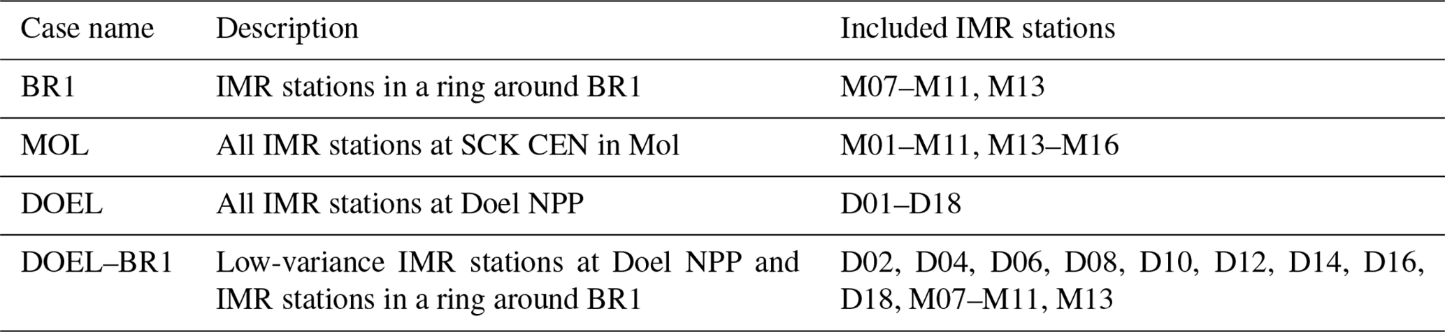
Posterior predictive distributions, plotted in Fig. 2, are a powerful tool to test the quality of Bayesian models. In all four cases, the close agreement between the black lines (observations) and orange lines (model) shows that the multivariate normal distribution is an excellent parameterisation for the distribution of the ambient dose equivalent rate vector $\mathbf{M}/T$. It shows that even if some detectors experience much higher local dose rates – the rightmost peak for the MOL case (Fig. 2b) corresponds to detector M06, which is adjacent to radioactive waste storage – the way that they covary can still be captured with a multivariate normal distribution. Likewise, it does not matter that some detectors are of a different make – the much wider central peak for the DOEL case (Fig. 2c) is due to the larger intrinsic variance of some of the detectors.

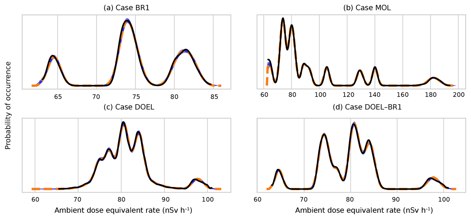
Figure 2 Posterior predictive distributions for all four analysed cases. Solid blue lines represent predicted distributions of observations. Each line is made by randomly drawing a set of parameters from the posterior distributions of parameters. Dashed orange lines represent the mean predicted distributions. Finally, the distribution of actual observations is represented in black – a kernel is used for interpolation to a continuous distribution.

The quality of the Bayesian model also becomes clear using the predictive formalism described in Sect. 2.3. Using the original training data but leaving out one or more detectors, the conditional distribution can be used to “predict” the observations by the excluded detectors. Here, we show the results for two cases: BR1 and DOEL. For the BR1 case, we predict the observations by M13 using observations by M07 through M11. Results of these “predictions” versus actual observations are plotted in Fig. 3. Again, the agreement is excellent. The calibrated model correctly captures not only the offset and the diurnal variations but also the generally rising trend. Moreover, the 1σ (68 % confidence) and 2σ (95 % confidence) intervals predicted by the model match the spread of the observations very well. This shows that the model captures not only the trends but also remaining uncertainties.

Figure 3 A prediction of detector M13 based on observations by M07 through M11. Time indices denote consecutive 10 min periods starting at 00:00 CEST on 6 August 2022 and ending at 00:00 CEST on 14 August 2022.

For the DOEL case, we predict the observations by D01 through D09 using observations by D10 through D18. These results are plotted in Fig. 4. The even-numbered stations have similar characteristics to the detectors around BR1. While offsets vary, the diurnal fluctuations, rising trend, and approximate uncertainties do not vary much between these detectors and their BR1 counterparts. Meanwhile, the odd-numbered detectors have almost an order of magnitude more uncertainty compared to the even-numbered detectors – likely owing to considerably worse counting statistics – in their model predictions, which is in excellent agreement with the actual spread in the TELERAD time traces, as evidenced by the fact that the shaded areas in Fig. 4 (which represent the uncertainty in the measurements) are much larger for the odd-numbered than for the even-numbered detectors. There is no evidence of diurnal variations or the rising trend any more, as these are dwarfed by the uncertainty inherent in the detectors. We observe that the predictions by the Bayesian algorithm are not impacted. The algorithm simply sets S_l of those detectors to high values while setting R_lm to low values so that the covariance with other detectors, S_lS_mR_lm, remains low.

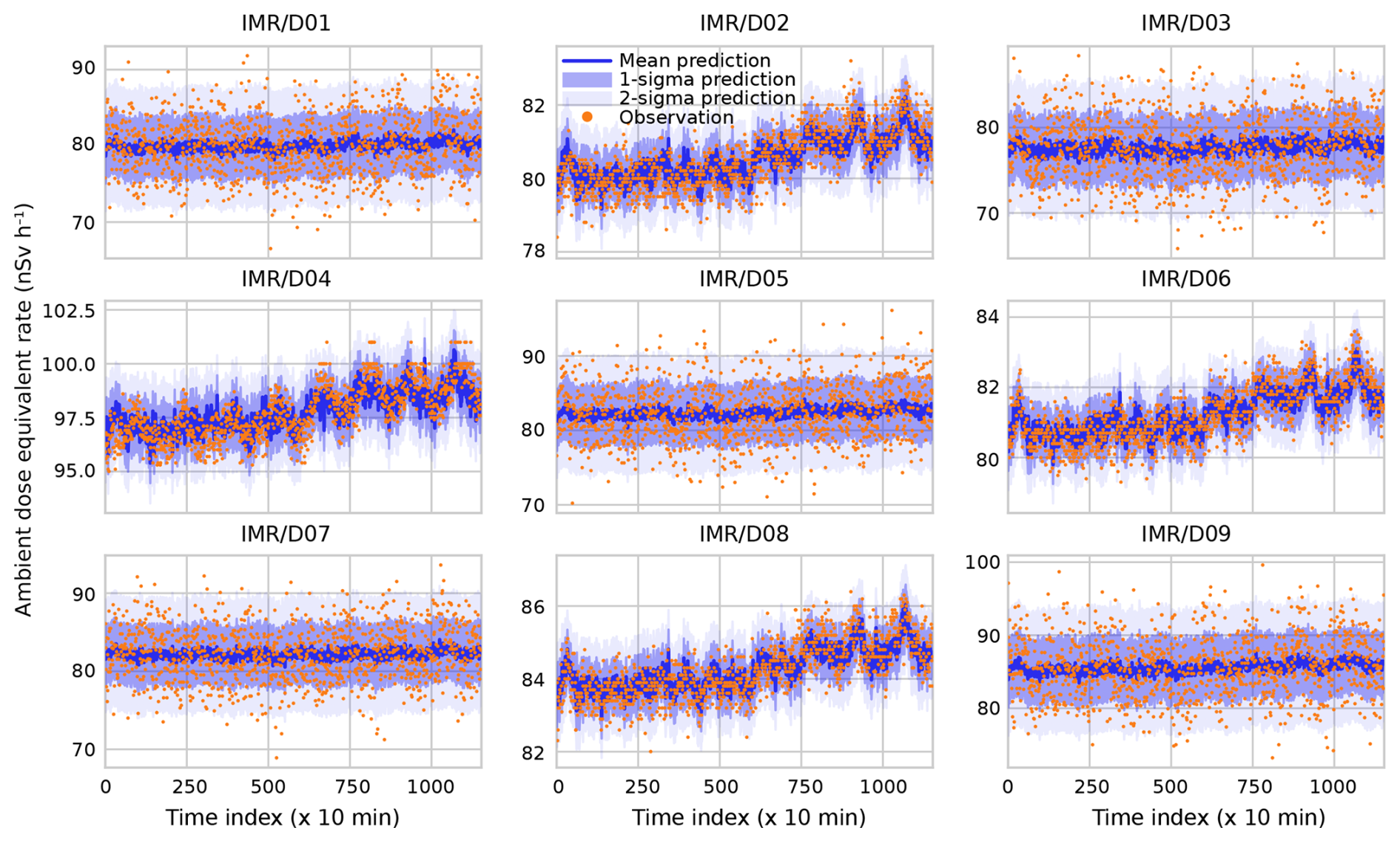
Figure 4 Predictions for the Doel detectors D01 through D09 based on observations by D10 through D18. Time indices denote consecutive 10 min periods starting at 00:00 CEST on 6 August 2022 and ending at 00:00 CEST on 14 August 2022.

4 Predictions using the conditional distribution

Using the calibrated models described in Sect. 3, trained on data between 6 and 13 August 2022, we now make predictions using data that were obtained at a different point in time in order to validate our Bayesian model. Here, we present the results for two cases, MOL and DOEL, for 10–12 September 2022. We start with the former. Similarly to the BR1 case, we exclude detector M13 and try to predict observations made by that detector using the other detectors as inputs. We then compare the prediction to the actual observations. The results can be found in Fig. 5. Focusing first on days two and three (from time index 150 onwards), the calibrated model predicts both the baseline dose rate and the peaks (around 200 and 350, so around dawn) quite well, while the variance appears to be slightly overestimated over the entire period. This is confirmed by comparing the mean of the 1 h running variances of the TELERAD data, $(\mathrm{0.15}\pm \mathrm{0.10}){\mathrm{nSv}}^{\mathrm{2}}{\mathrm{h}}^{-\mathrm{2}}$, to the mean of the predicted variances, $(\mathrm{0.21}\pm \mathrm{0.01}){\mathrm{nSv}}^{\mathrm{2}}{\mathrm{h}}^{-\mathrm{2}}$ (excluding time indices smaller than 100 because of the rain peak).

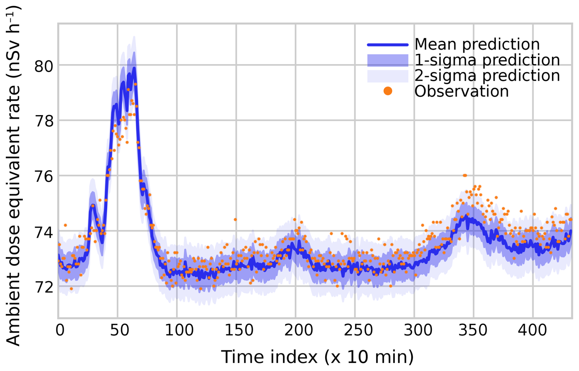
Figure 5 Prediction of the dose rate measured by detector M13 based on observations by the other detectors on the SCK CEN site. Time indices denote consecutive 10 min periods starting at 00:00 CEST on 10 September 2022 and ending at 00:00 CEST on 13 September 2022, so three diurnal cycles are included in the prediction. The larger peak between time index 25 and 75 coincided with a period of precipitation.

Most striking in Fig. 5 is the larger peak between time indices 25 and 75. It coincides with a period of precipitation measured by the station in Retie (Vlaamse Milieumaatschappij, 2023), which is known to coincide which rising dose rates (Mercier et al., 2009; Livesay et al., 2014). While our model was not trained on precipitation data, the match is nonetheless quite good. It appears that over the extent of the Mol site, precipitation has the same effect as other meteorological drivers (e.g. pressure), which cause the variations over time observed in Figs. 3 and 4. However, that does not mean that our choice of parameterisation is ideal in precipitating conditions: part of the variance in such cases might be driven by, for example, fluctuations in the precipitation rate, which may not necessarily be Gaussian. Moreover, that our model can describe the effect of precipitation has a downside in an operational context. A plume (cloud) of radioactivity that is released far enough from the site is homogeneously distributed over the site and cannot be distinguished from other background effects by on-site detectors. Our model is thus only useful to spot aberrant radioactivity at a typical scale that is smaller than that of the network, i.e. local releases.

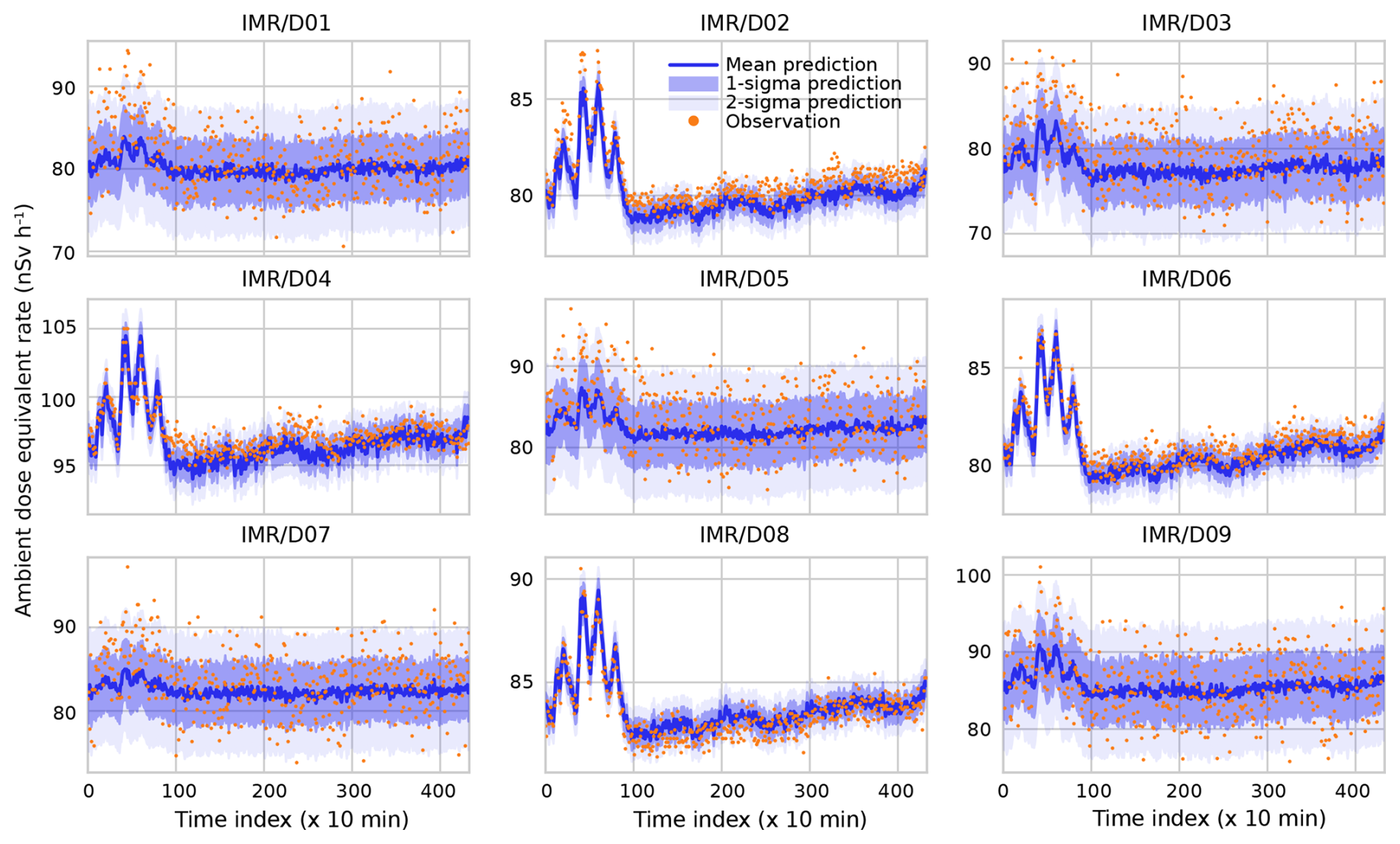
Figure 6 Prediction of the dose rate measured by detectors D01 through D09 based on observations by detectors D10 through D18. Time indices denote consecutive 10 min periods starting at 00:00 CEST on 10 September 2022 and ending at 00:00 CEST on 13 September 2022, so three diurnal cycles are included in the prediction.

Next, we present the DOEL case. Based on the observations made by detectors D10 through D18, the calibrated model predicts the observations by D01 through D09. The results are plotted in Fig. 6. Overall, the same conclusions can be drawn as for the MOL case. The precipitation peak, although a fair bit more jagged than before, is still resolved well. Some limited drift on the mean vector μ is present, and small under- or overestimations are present for some of the detectors. The fluctuations in the dose rates are still captured well however. That there should be a drift in the vector of means is interesting and suggests the involvement of a process that causes decorrelation in time. Such a process cannot be modelled under the assumptions presented in our work because we have chosen to neglect temporal correlations. Moving from a temporally independent model into, for example, a first-order Markov system would increase the dimensionality of the joint probability density function (pdf) from k² to (2k)². This would have significant computational repercussions and may not be feasible.

In the special case of the multivariate normal distribution presented in this work, solutions might exist (e.g. Kalman filtering). However, by moving to the Kalman filter approach, one loses the option to move away from the normality assumption at a later stage – this could be a problem, potentially, when introducing the effect of precipitation. An alternative that would not necessitate moving away from the Bayesian inference method would be to serve the calibrated coefficients of the background model as a prior in the predictive step and to allow small posterior updates to the vector of means to correct for drift.

5 Predictions during operation of BR1

Finally, we present simulations for the DOEL–BR1 case between 30 August and 1 September 2022. To expedite the calibration and prediction steps, we only include the even-numbered detectors in Doel. As can be seen in Figs. 4 and 6, these detectors have a considerably higher dose rate resolution than their odd-numbered counterparts and hence contain much more information. The results are shown in Fig. 7. The match between the background prediction and the actual observations is poor during several intervals which coincide with operation of BR1. BR1 was operational between approximately 09:00 and 16:00 CEST in this 3 d period (time indices 54–96, 198–240, and 342–384). Outside of those intervals, the predictions by our model and the observations match very well.

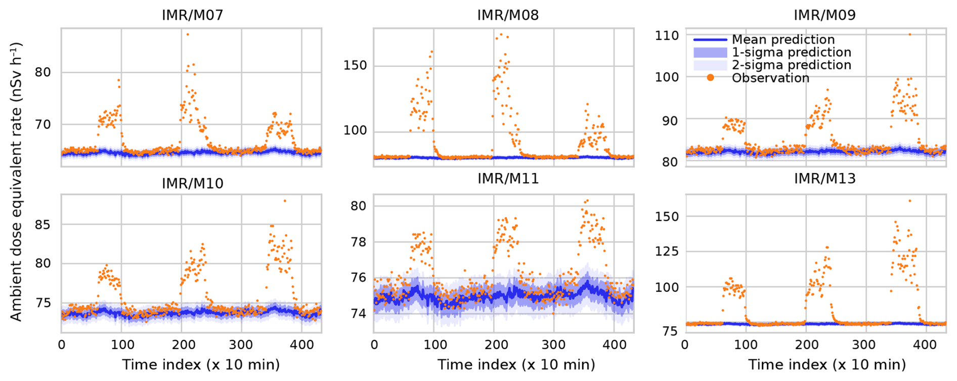
Figure 7 Prediction of the dose rate measured by the BR1 ring detectors (M07 through M11 and M13) using as inputs measurement by the even-numbered Doel detectors. Time indices denote consecutive 10 min periods starting at 00:00 CEST on 30 August 2022 and ending at 00:00 CEST on 2 September 2022, so three diurnal cycles were included in the prediction. During this period, BR1 was turned on for 3 d on end, which is apparent from the three large peaks that are not described by the background model prediction.

It is perfectly possible to describe the effect that BR1 – which is an air-cooled reactor that emits argon-41 during operation – has on the detectors using atmospheric dispersion modelling (Frankemölle et al., 2022b). However, because it is an effect that varies over a characteristic length scale that is much smaller than that of the network (ca. 50 km here), it cannot be captured by our background model. This is exactly where our background modelling can be useful for spotting anomalies. To quantify the size of the anomaly, a good estimate of the background level can be crucial, particularly for smaller atmospheric releases. While small errors in the mean and the intrinsic variance of the background are largely irrelevant for large anomalies (e.g. M08), they are relevant in situations where both effects are of the same order (e.g. M11). When release levels are even lower and occur during a much shorter interval – as was the case for the selenium-75 incident at SCK CEN for example (Frankemölle et al., 2022a) – a good understanding of the background becomes even more critical.

6 Conclusions and outlook

In this work, we presented a Bayesian inference framework for background estimation in densely packed local detector networks. We treated the background ambient dose equivalent rate observed in a dense detector network as a multivariate stochastic vector. We derived a physics-informed likelihood – a multivariate normal distribution – and priors and used these to calculate the posterior pdf's of several parameters of interest. Using data from the Immission Monitor for the Ring area (IMR) sub-network, part of the TELERAD network (Sonck et al., 2010), on the sites of the Belgian Nuclear Research Centre in Mol (SCK CEN) and the Doel nuclear power plant (NPP) in Belgium, we then put the Bayesian framework to the test.

In Sect. 3, we validated the suitability of our chosen parameterisation. That this parameterisation was a suitable choice became clear from the posterior predictive checks. The actual distribution of the observations matched very well with the modelled distribution of observations. Moreover, leave-one-out and leave-many-out checks, which leveraged the conditional distribution, were successfully used to reconstruct the training data. In Sect. 4, actual leave-one-out and leave-many-out predictions were made using new observational data in combination with a model that was calibrated using month-old training data. While the model predictions had drifted away slightly from the actual observations, the calibration overall proved to be rather stable. Diurnal fluctuations were reproduced well, and the short-term variance was matched decently. Finally, Sect. 5 showed an application of our model where detectors at Doel NPP were used to predict the observations by detectors at SCK CEN during operation of BR1. This application demonstrates the relevance of our work in the field of anomaly detection and, importantly, quantification.

Looking at the model from an operational perspective, the slow drift of the mean vector away from its calibration precludes usage of year-old calibrated models. However, the drift within a month is only very limited, so if the Bayesian model were recalibrated every week using the latest available data – which is possible thanks to the limited computational cost – the drift should not be a problem. In fact, the model itself could be used to automatically determine whether next week's data are suitable for recalibration (which amounts to checking whether no anomalies are present). Of course, in the specific case of SCK CEN – with regular anomalies due to BR1 – finding non-anomalous data can be problematic. In this case, coupling to a near-range atmospheric dispersion model is likely necessary. This would also require extending the Bayesian framework to include additional uncertainties arising from the dispersion modelling. Ideally, a similar provision would be made for precipitation, which – as discussed in this work – might come with its own temporal and spatial uncertainties.

Finally, future work could include a temporal correlation to the parameterisation of the background vector, but care should be taken that the computational complexity does not get out of hand. Should the multivariate normal distribution that was used in this work remain the best fit for the job, then recasting this work into a Kalman filter formulation might do much to alleviate these issues. Conversely, rather than taking the calibration as fixed, the vector of means might be updated as part of the prediction process, i.e. formalising the recalibration process described in the previous paragraph. The posterior obtained by calibration on training data then becomes a prior for the prediction data.

Appendix A: Bayesian inference

To describe the detector networks, we use statistical inference. Statistical inference is the process of inferring the properties of a population from a limited sample or, in other words, the process of determining the probability distribution of a stochastic (random) variable (SV) from a limited number of observations of that SV. Statistical inference comes in two flavours: the Bayesian and the frequentist. Bayesian approaches treat the properties of a population as intrinsically random SVs in turn, whose distributions are constrained by the available observations and by a subjective belief, while frequentist approaches treat them as fixed values that can be determined up to some uncertainty threshold based solely on the available data (Pishro-Nik, 2014). In our work, we take the former perspective. The simplest form of Bayes's theorem, which can be found in statistics handbooks (e.g. Pishro-Nik, 2014; Hogg et al., 2018), is

$$\begin{array}{}\text{(A1)}& P_{X|Y}\left(x\right|y)={\displaystyle \frac{P_{Y|X}\left(y\right|x\left)P_X\right(x)}{P_Y\left(y\right)}},\end{array}$$

which defines the posterior probability mass function $P_{X|Y}\left(x\right|y)$ as the product of the likelihood function $P_{Y|X}\left(y\right|x)$ and the prior probability mass function P_X(x) over the marginal likelihood function P_Y(y). They are usually simply referred to as the posterior, likelihood, prior, and evidence. The subscripts X and Y are SVs, and X=x and Y=y are realisations of those SVs. When dealing with multiple unknowns, SVs generalise to stochastic (random) vectors whose elements are SVs. Rather than with X and Y, we then deal with $\mathit{X}=[X_{\mathrm{1}},\mathrm{\dots },X_k{]}^{\top }$ and $\mathit{Y}=[Y_{\mathrm{1}},\mathrm{\dots },Y_k{]}^{\top }$ with realisations $\mathit{x}=[x_{\mathrm{1}},\mathrm{\dots },x_k{]}^{\top }$ and $\mathit{y}=[y_{\mathrm{1}},\mathrm{\dots },y_k{]}^{\top }$. Moreover, when dealing with continuous rather than discrete SVs, probability mass functions P (pmf's) become probability density functions f (pdf's). The multivariate formulation of Bayes's theorem for continuous stochastic vectors finally reads

$$\begin{array}{}\text{(A2)}& f_{\mathit{X}|\mathit{Y}}\left(\mathit{x}\right|\mathit{y})={\displaystyle \frac{f_{\mathit{Y}|\mathit{X}}\left(\mathit{y}\right|\mathit{x}\left)f_{\mathit{X}}\right(\mathit{x})}{f_{\mathit{Y}}\left(\mathit{y}\right)}},\end{array}$$

where the posterior, likelihood, prior, and evidence are now joint pdf's. Since, in the current work, we are always dealing with joint pdf's, we often refer to them as joint distributions or even simply as distributions.

Formally, we should always distinguish between stochastic variables and vectors (X and X) and their realisations (x and x). However, this makes notation cumbersome and does not always add much in the way of clarity, so in the main text we often ignore the difference.