A new global high-resolution wave model for the tropical ocean using WAVEWATCH III version 7.14

Climate change is driving sea-level rise and potentially intensifying extreme events in the tropical belt, thereby increasing coastal hazards. On tropical islands, extreme sea levels and subsequent marine flooding can be triggered by cyclones but also distant-source swells. Knowledge of sea states in the tropical ocean is thus of key importance, and their study is usually based on spectral wave models. However, existing global wave models typically employ regular grids with a coarse resolution, which fail to accurately represent volcanic archipelagos, a problem usually circumvented by the use of obstruction grids but typically resulting in large negative biases. To overcome this problem, this study presents a new global wave model with a focus on distant-source swells, which have received less attention than waves generated by cyclones. To accurately simulate sea states in tropical areas, we implemented the spectral wave model WAVEWATCH III© (WW3) over a global unstructured grid with a spatial resolution ranging from 50 km to 100 m. The model is forced by ERA5 wind fields, corrected for negative biases through a quantile–quantile approach based on satellite radiometer data. The wind input source terms adjusted accordingly and the explicit representation of tropical islands result in improved predictive skills in the tropical ocean. Moreover, this new simulation allows for the first time direct comparisons with the in situ data collected on volcanic islands at water depths ranging from 10 to 30 m, which corresponds to a few hundred meters from the shore.

1 Introduction

Over the last few decades, coastal hazards have increased due to climate change, which causes sea-level rise and a possible intensification of extreme events in the tropical belt that can lead to more frequent marine flooding (Oppenheimer et al., 2019). Recent studies have even suggested that some low-lying islands and atolls could become uninhabitable by 2060–2090 due to annual flooding (Giardino et al., 2018). In addition, rising sea surface temperatures and ocean acidification exert strong pressure and locally degrade coral reefs, increasing the exposure of coastal islands to extreme events (Gattuso et al., 2014).

On tropical islands, extreme sea levels commonly result from storm surges, driven by the combination of atmospheric perturbations associated with tropical cyclones with a wave setup due to wave dissipation over reefs (Kennedy et al., 2012). Extreme sea levels can also develop apart from cyclones due to distant-source swells (hereafter DSSs) (Hoeke et al., 2013). DSSs are generated by remote storms developing several thousand kilometers away from the tropical belt, with the resulting DSSs then propagating toward tropical coasts (Munk et al., 1997; Delpey et al., 2010; Smithers and Hoeke, 2014). DSSs are less studied than cyclonic waves, but their importance to coastal hazards has been demonstrated at several tropical islands such as the island of Réunion (Lecacheux et al., 2012), French Polynesia (Canavesio, 2019; Andréfouët et al., 2023), Hawai′i (Stopa et al., 2016), the Marshall Islands (Ford et al., 2018; Giardino et al., 2018) and the British Virgin Islands (Cooper et al., 2013). It is worthwhile to highlight that, in contrast to cyclonic events associated with strong local winds and a drop in atmospheric pressure, strong DSS events are able to impact and damage the shore by physical processes solely driven by wave action (wave setup, wave-driven currents, direct wave impact or long wave generation).

To accurately represent the propagation of DSSs over thousands of kilometers, from the swell source in high latitudes to the tropical oceans, global spectral models are nowadays the most efficient approach. Spectral models describe the space and time evolution of the wave energy spectrum, using a phase-averaged approach that typically employs a resolution of tens of kilometers in the deep ocean. However, the accurate representation of the wave field around and within archipelagos made up of islands only a few kilometers wide requires us to reach a much finer resolution. To simulate the effect of small islands on the wave field while keeping computational times acceptable on a global scale, two approaches were developed. The first one uses an obstruction mask technique, which is only applicable to structured grids. In this approach, the percentage of land within each cell is used as a coefficient to calculate the attenuation of the wave action flux through the considered cell (Tolman, 2003). The second approach is based on a source term that considers both the attenuation of the wave action flux through the considered cell and its shadowing effect on the downstream cells. This method can be used for structured and unstructured grids (Mentaschi et al., 2018).

However, state-of-the-art hindcasts usually exhibit substantial negative biases around archipelagos, suggesting that these techniques result in excessive wave energy loss (Rascle and Ardhuin, 2013; Dutheil et al., 2020). To overcome this issue, models using unstructured grids present an interesting potential since they allow small islands to be explicitly represented by locally refining the mesh. Unstructured grids were first applied using explicit schemes, but the resulting high computational cost restricted this approach to regional areas (Roland, 2008; Roland and Ardhuin, 2014; Monteiro et al., 2022). Through the adoption of implicit schemes, which enable the Courant–Friedrichs–Lewy (CFL) constraint to be overcome and significantly reduce simulation duration (Abdolali et al., 2020), unstructured grids slowly started to be used at a global scale (Brus et al., 2021; Mentaschi et al., 2023). Yet, the spatial resolution used in these studies remains too coarse to allow for a direct validation around volcanic tropical islands because available in situ data, coming from wave buoys or bottom-moored pressure sensors, are usually located very close to shore (i.e., less than 1 km) due to the steep seabed slope around islands. Aiming to improve our capacity to accurately simulate sea states in tropical areas, we set up a new global spectral wave model based on an unstructured grid with a resolution ranging from 50 km to 100 m. Such fine resolution is set to allow for direct comparisons with measurements available at a water depth of 10–30 m, which is very close to shore. The subsequent sections of this paper are structured as follows. First, we describe the spectral wave model, its implementation, and the observational data used for model validation at global and coastal scales. Section 3 highlights the model improvements through wind field corrections and the explicit representation of small islands both in the deep ocean and nearshore. Finally, we discuss the added value and limitations of the present approach, including the remaining challenges associated with spectral wave modeling on unstructured grids in tropical areas.

2 Material and methods

2.1 Global wave models

2.1.1 Model description

Spectral wave models such as WAVEWATCH III© (WW3 Development Group, 2019) are typically used for large-scale applications, including for operational or academic purposes. Spectral models are increasingly being applied to coastal areas, thanks to the development of unstructured grid versions, the better representation of coastal physics, and the development of adaptive numerical schemes and integration strategies. In this work, we evaluate the performance of the model in simulating the sea states in the tropical ocean using version 7.14 of WW3.

WW3 calculates the evolution of the wave spectrum by solving the wave action equation (Komen et al., 1996). The source terms of this equation represent several key processes involved in wave transformation. In deep water, wave generation by wind (S_in) and wave dissipation by whitecapping (S_ds) are computed according to Ardhuin et al. (2010). Nonlinear wave interactions (S_nl) are modeled using the discrete interaction approximation (DIA) of Hasselmann et al. (1985). The representation of wave–sea ice interactions follow Liu and Mollo-Christensen (1988), Liu et al. (1991), and Ardhuin et al. (2015) for wave damping by ice (S_ice) and the approach of Moon et al. (2007) for scattering and dissipation by sea ice (S_is). In shallow water, three other source terms become important: wave dissipation by bottom friction (S_bot), represented here using the SHOWEX parameterization of Ardhuin et al. (2003); breaking-induced wave dissipation (S_db), which follows the formulation of Battjes and Janssen (1978); and nonlinear triad interactions modeled using the LTA model of Eldeberky (1996). For structured grids, the spatial propagation is solved using the explicit third-order Ultimate Quickest scheme (Leonard, 1991). This scheme is robust and stable but is limited by the CFL constraint, which discards the possibility of employing a spatial resolution fine enough to capture nearshore wave transformations at a global scale. Implicit schemes can be used to avoid prohibitive calculation costs at a regional scale while maintaining good scalability (e.g., Booij et al., 1999) on large cores and mesh refinement. The WW3 implicit scheme, used in many studies and operational applications (e.g., Abdolali et al., 2020, 2021; Alves et al., 2022), computes a non-split solution of the wave action equation using a block Gauss–Seidel (Ferziger and Peric, 2002) solver for source terms and advection, avoiding splitting errors associated with the usual fractional step method. Recently, the integration methods and the numerical limiter were reformulated following Hersbach and Janssen (1999). Under-relaxation (e.g., Moukalled et al., 2016) for the strong and nonlinear terms describing near-resonant triplet interactions and shallow-water-induced wave breaking was added. Additional improvements on parallelization were implemented (Roland, 2008; Abdolali et al., 2020). Here we use the domain decomposition methods based on ParMETIS (Karypis, 2011), which is interfaced using the Parallel Domain Decomposition Library (PDLIB).

2.1.2 Model implementations

Two grids are implemented to assess the relevance of a new unstructured grid compared to a classical structured grid.

The unstructured grid (hereafter UG) is created using the Surface-water Modeling System (SMS; Aquaveo, 2014). The mesh totals 296 199 nodes, with a resolution ranging from 50 km in the deep ocean to about 1 km around most islands (Fig. 2). Around the selected validation sites (see Sect. 2.2.2), the spatial resolution ranges from 1000 to 500 m. At Réunion, where pressure transducer data are available only 400 m from the shoreline, the spatial resolution was further refined to 100 m. Such a fine resolution allows the water depth in the model to match that of the pressure transducer, which is essential for providing a consistent comparison. All islands smaller than 10 km² were arbitrarily removed to limit CPU time. The periodic continuity between −180 and 180° is guaranteed through the modification of the grid connectivity table.

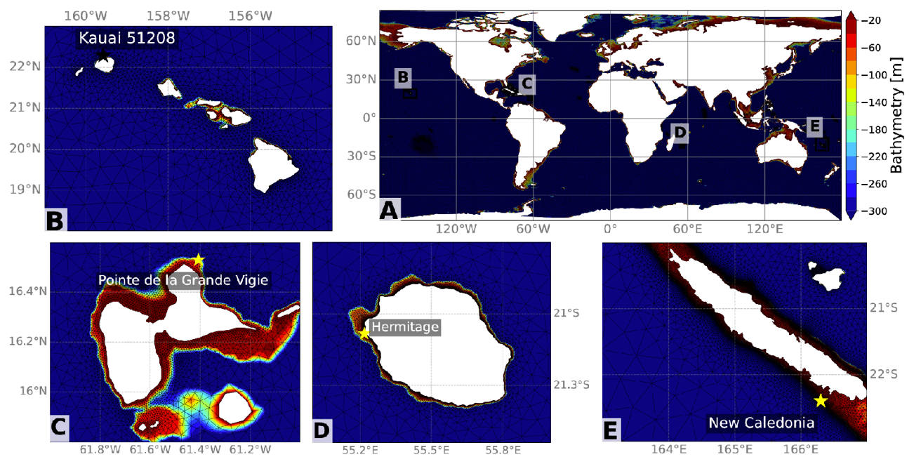
Figure 1 The global unstructured grid (a) with refinement in Hawai′i (b), Guadeloupe (c), Réunion (d) and New Caledonia (e). The bathymetry is represented by the color legend.

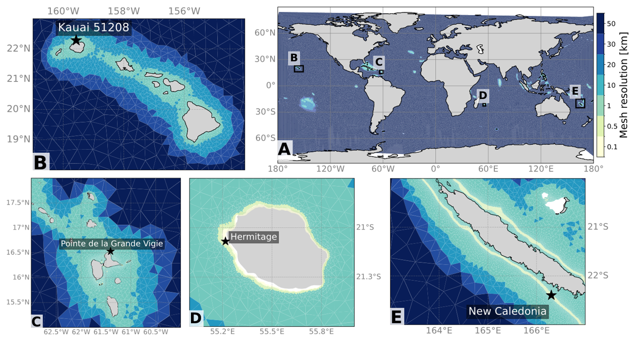
Figure 2 The global unstructured grid (a) with refinement in Hawai′i (b), Guadeloupe (c), Réunion (d) and New Caledonia (e). The mesh resolution is represented by the color legend.

The structured grid (hereafter SG) has a uniform global resolution of 0.5°, and islands smaller than the cell size are represented with an obstruction grid (Rascle and Ardhuin, 2013). The spectral grid consists of 24 directions and 36 frequencies logarithmically spanning the range 0.035–1.01 Hz (meaning a frequency interval exponent of 1.1). For SG, time steps are set to 1350 s for global, 450 s for geographic advection and 600 s for spectral advection. The minimum time step for source term integration is 35 s. For UG, the implicit scheme does not require any splitting, and a time step of 800 s is set. The global bathymetry comes from the General Bathymetric Chart of the Oceans (GEBCO) dataset (Weatherall et al., 2015). For UG, a higher-resolution bathymetry is used around French tropical islands (New Caledonia, Réunion, Mayotte, French Polynesia, West Indies), originating from the digital elevation models of HOMONIM of 100 m resolution (Biscara and Maspataud, 2018).

Wind and ice forcing comes from the ERA5 reanalysis (Hersbach et al., 2020) with a 3 h time resolution and a spatial resolution of 0.5° globally. ERA5 also offers hourly data, but sensitivity tests revealed similar results with 3 h wind fields. The ERA5 winds were preferred to the CFSR winds as they are more consistent over time (Liu et al., 2021). However, ERA5 winds are known to exhibit strong negative biases for the strongest winds (Pineau-Guillou et al., 2018; Campos et al., 2022). To solve this issue, Alday et al. (2021) proposed a correction of 5 % of the wind speeds above 20 m s⁻¹ and a new parameterization of the source term in WW3 where the betamax parameter, which controls the wave generation by the wind, is adjusted to 1.75. Our initial tests have shown that this approach reproduces the most energetic sea states well but results in positive biases for calmer conditions. Given that ERA5 winds are unbiased for light to moderate winds, we developed an alternative strategy, where wind fields are corrected using a quantile–quantile approach, based on wind field estimates from radiometers as described by Bentamy and Croize-Fillon (2012), available since 1992. The proposed correction is based on a piecewise multiplication factor displayed in Table 1.

Table 1 Wind speed and correction factor calculated through a quantile–quantile approach, based on wind field estimates from radiometers.

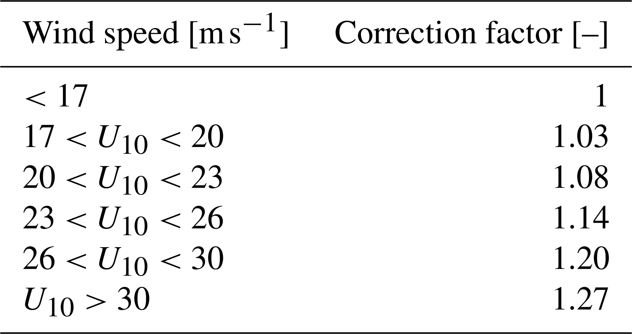
ERA5 wind fields were compared against radiometer data over different oceanic basins (Pacific, Indian, Atlantic) for selected 1-month periods (July 1996, May 2007, January 2014, respectively), encompassing major past swell events and enhanced very strong winds. In the southern Pacific Ocean, a major storm in July 1996 produced one of the largest distant swells ever reported (Canavesio, 2019), with wind fields reaching 30 m s⁻¹ (Fig. 3c). In the southern Indian Ocean, a strong storm in May 2007 produced winds over 30 m s⁻¹ (Fig. 3b), which drove a major distant swell (Lecacheux et al., 2012). Finally, in the NE Atlantic Ocean, the winter of 2014 exhibited an unprecedented succession of violent storms (Masselink et al., 2016), with several events driving winds over 35 m s⁻¹ (Fig. 3a). For these three periods and regions, the comparison confirms that ERA5 winds are unbiased for speeds up to 15 m s⁻¹, while for higher winds, the bias correction reaches 10 % at 20 m s⁻¹ and 15 % at 25 m s⁻¹. Remarkably, this correction holds for all oceanic basins and time periods where the comparison is performed. Finally, the “Test471” parameterization of Rascle and Ardhuin (2013) is used for the wind growth and whitecapping dissipation source terms, where the betamax parameter has been adjusted to 1.43. The new parameterization proposed in this study is hereafter called “ERA5_QC”.

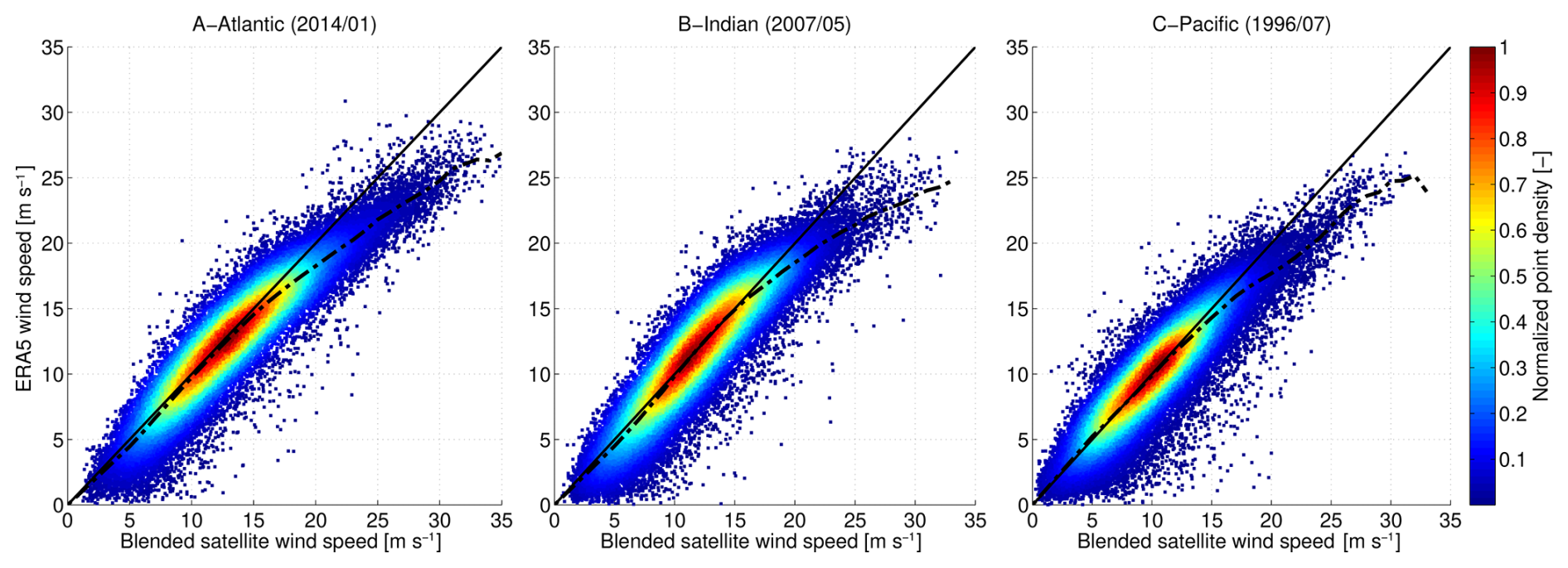
Figure 3 Comparisons between blended winds and ERA5 winds for (a) the Atlantic ocean, (b) the Indian Ocean and (c) the Pacific Ocean.

Other source terms are set to default settings.

2.2 Observational data

Altimetry data and in situ measurements are used for global and coastal validation, respectively.

2.2.1 Altimetry data for global validation

The model evaluation in the deep ocean is performed against the European Space Agency Climate Change Initiative (ESA CCI) altimetry data (Dodet et al., 2020; Schlembach et al., 2021). The ESA CCI v3 dataset used here was retrieved from multiple satellite missions spanning 2002 to 2022. For the present model validation, an entire year (2007) is used to cover a wide range of sea states. The simulated significant wave height H_m0 over the full spectral range is interpolated in time and space to match the satellite “denoised” significant wave height at approximately 6 km spatial resolution (Quilfen and Chapron, 2021; Schlembach et al., 2021). Both satellite data and interpolated WW3 outputs are averaged over 0.5° grid cells, which enables us to calculate stable statistical values for the collocated satellite and model data. All satellite values outside of the model time and space ranges were skipped. Coastal values in a 50 km range from the shoreline were flagged due to possible coastline interference with the signal and the lack of model resolution along the coast.

2.2.2 Coastal and nearshore data

For each coastal/nearshore site, the model validation is performed over a 4-month period, selected to represent a wide variety of wave conditions. The WW3 wave bulk parameters (H_m0 and T_m02) are calculated from the modeled spectrum using a specific frequency cut-off, depending on the water depth or the device employed (see Table 2). For bottom pressure data, the nonlinear moderately dispersive reconstruction described by Martins et al. (2021) is employed. Wave bulk parameters are then computed using classical spectral analysis.

Table 2 Description of coastal and nearshore data used for model validation at the four study sites.

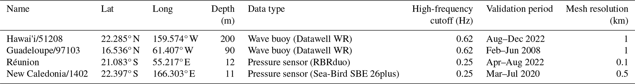
For Hawai′i (Pacific Ocean), the validation data are provided by the 51208 wave buoy from the National Data Buoy Center (NDBC), and the period from August to December 2022 was chosen due to the occurrence of highly energetic events. The data are owned and maintained by the Pacific Islands Ocean Observing System (PacIOOS) and provided by the Scripps Institution of Oceanography. The buoy is located above Hanalei Bay, to the north of Kauai at 200 m water depth (see Fig. 1b). For this buoy, only H_m0 and T_p time series were available.

For Guadeloupe (Atlantic Ocean), the validation data are collected by the 97103 Candhis wave buoy from the Centre d'études et d'expertise sur les risques, l'environnement, la mobilité et l'aménagement (CEREMA) and Météo-France. The period from March to July 2008 was chosen for validation due to the occurrence of an extreme swell event (Lefèvre, 2009). The buoy is located in the French West Indies, above the Pointe de la Grande Vigie, northeast of Guadeloupe at 90 m water depth (see Fig. 1c).

For Réunion (Indian Ocean), the pressure sensor data are collected continuously in the framework of the Service National d’Observation (SNO) DYNALIT, and the SNO ReefTEMPS-OI (Cordier et al., 2024), which are part of an instrumented site of the research infrastructure ILICO. The period from April to August 2022, during which a strong swell event occurred, was chosen for validation. The pressure sensor is located in the reef slope in front of Hermitage Beach, bottom moored by a mean water depth of 12 m (see Fig. 1d).

For New Caledonia (Pacific Ocean), pressure sensor data were collected from October 2019 to November 2020 during the GEOCEAN-NC 2019 field campaign (Chupin et al., 2023). The pressure sensor was moored in the reef slope to the southwest of the main island by a mean water depth of 11 m (see Fig. 1e). The period from March to July 2020 was chosen for validation as it encompasses several energetic events.

Lastly, as the 3 h resolution of the wind forcing does not allow us to capture the high-frequency wave variability, observational data were low-pass filtered with a 3 h window.

2.3 Validation metrics

Several metrics are used to assess the errors between modeled results and observational data, including the normalized mean square error (NRMSE) defined as

$$\begin{array}{}\text{(1)}& \text{NRMSE}\left(X\right)=\sqrt{{\displaystyle \frac{\sum (X_{\text{mod}}-X_{\text{obs}}{)}^{\mathrm{2}}}{\sum X_{\text{obs}}^{\mathrm{2}}}}},\end{array}$$

where X_mod is the modeled result and X_obs the observed value. The normalized bias is defined as

$$\begin{array}{}\text{(2)}& \text{NBIAS}\left(X\right)={\displaystyle \frac{\sum (X_{\text{mod}}-X_{\text{obs}})}{\sum X_{\text{obs}}}}.\end{array}$$

3 Results

3.1 Global validation in deep water

The model validation in deep water is first performed only on structured grids to evaluate the effect of wind field correction. Next, the evaluation of the spatial discretization is carried out comparing SG and UG approaches, both including the wind correction.

3.1.1 Impact of wind field correction

Initial results with the parameterization T475 of Alday et al. (2021) on SG show a global mean NRMSE of 14.1 % and a global positive bias of 3.36 % (see Fig. 4a). Around island archipelagos (e.g., French Polynesia, Indonesia, West Indies, Maldives), higher errors occur locally, exceeding 30 %. These larger errors are mostly associated with strong negative biases and are presumably linked to the obstruction grid. The implementation of the wind correction leads to better results, especially in the Atlantic, Indian and Pacific oceans, away from island areas, with a global NRMSE of 12.9 % (Fig. 4b). Strong positive biases are locally lowered, which results in a global mean normalized bias of −4.4 %.

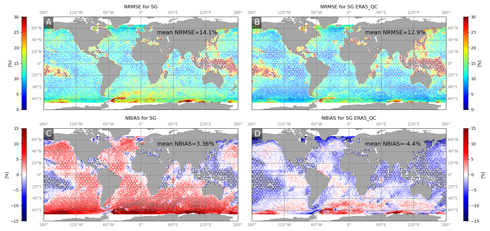
Figure 4 Normalized RMS error (a) and normalized bias (c) between H_m0 deduced from altimetry and simulated with the T475 parameterization and normalized RMS error (b) and normalized bias (d) with the ERA5_QC parameterization.

3.1.2 Impact of spatial discretization: SG vs. UG

Figure 5 displays the comparison between SG and UG configurations, both employing ERA5_QC. The unstructured grid leads to a lower global NRMSE of 11.6 % (see Fig. 5b). Much stronger local improvements are observed around archipelagos all around the globe. In SG, tropical archipelagos are generally associated with large NRMSE and strong negative bias. In UG, NRMSE is drastically reduced, while the bias shifts to weakly positive. Restricting the NRMSE computation to the tropical band, between 23.27° N and 23.27° S, the error drops from 15.3 % to 11 % with the UG. The global mean normalized bias is considerably reduced to 1.5 % with the ERA5_QC parameterization.

The results obtained globally for the UG ERA5_QC configuration are further analyzed and discussed in Sect. 4, where we investigate the implications of the remaining biases and their potential sources, particularly focusing on regions such as Antarctica, semi-enclosed seas, coastlines, the Mozambique Channel and the inner seas of Indonesia where higher errors persist.

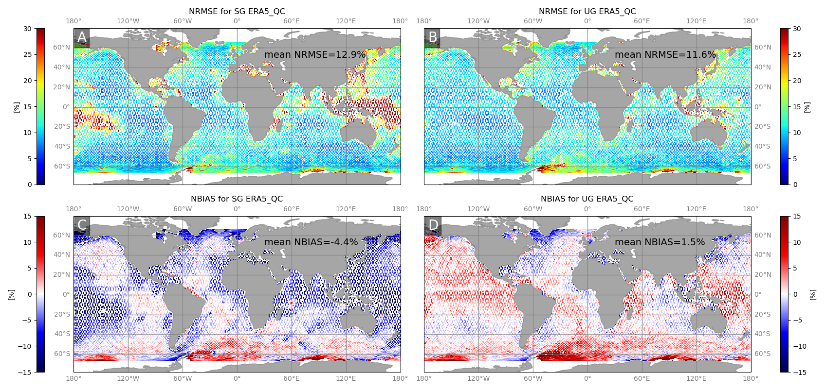
Figure 5 Normalized RMS error (a) and bias (c) between H_m0 deduced from altimetry and simulated with the UG ERA5_QC configuration and normalized RMS error (b) and normalized bias (d) with the SG ERA5_QC parameterization.

The distribution of the bias as a function of H_m0 is shown in Fig. 6 for the three model configurations. With SG, the ERA5_QC parameterization results in a lower bias compared to T475. Indeed, the T475 parameterization uses a higher betamax parameter, which controls the wind input term and hence the wave growth, set to 1.75 compared to 1.43 in the ERA5_QC parameterization. This higher betamax leads to greater wave growth and therefore a positive bias, although winds are lighter in T475 than in ERA5_QC. For the UG ERA5_QC, the bias is positive for H_m0 between 1 and 2.5 m, and the bias slowly decreases after and is negative for H_m0 values ranging from 2.5 to 12 m. The bias reaches its lowest value at −0.4 m for H_m0 of 11 m. The observed lower biases for the SG and the ERA5_QC models in the 10–12 m wave bins are discussed further in the paper.

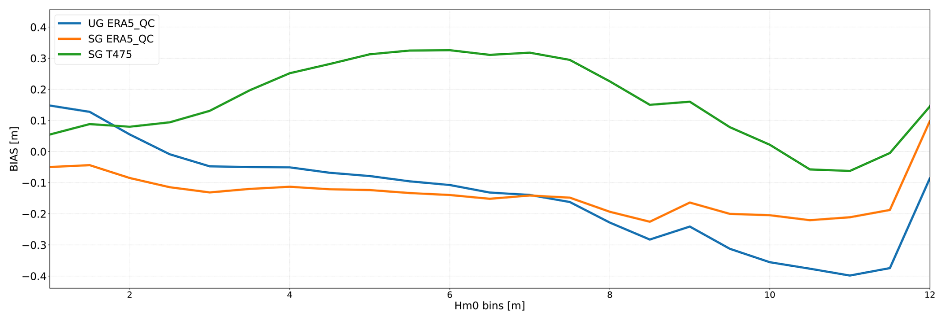
Figure 6 Distribution of the bias as a function of H_m0 for each simulation (SG T475, SG ERA5_QC and UG ERA5_QC) for the year 2007 at a global scale.

3.2 Example of coastal validation

Long-term in situ wave data are scarce in the nearshore area of tropical islands bordered by steep slopes. The coastal validation of the model is carried out at four tropical islands: Réunion in the Indian Ocean, Guadeloupe in the Atlantic Ocean, and New Caledonia and Kauai (Hawai′i archipelago) in the Pacific Ocean. These islands are representative of steep-slope tropical islands exposed to multi-modal sea states. For each island, in situ measurements are available at water depths ranging from 11 to 200 m for periods over 1 year, allowing us to evaluate the performance of a global wave model very close to shore for the first time.

3.2.1 Réunion

Figure 7 displays the comparison between model and bulk parameters computed from pressure sensor data at Réunion (12 m water depth) for H_m0, T_m02 and T_p. Overall, the model is able to capture the variability of the sea state over the selected time period, including the extreme DSS of 29 June 2022 where H_m0 reached 7 m with T_p exceeding 21 s. The NRMSE for H_m0 of 19.82 % is similar to the NRMSE obtained in the deep ocean around Réunion (see Fig. 5). The consistency between the results obtained globally and the results obtained in shallow water at Hermitage demonstrates the ability of the model to represent the wave transformation from the deep ocean to a shallow area. H_m0 tends to be slightly overestimated, which also matches the deep-water bias in this region (Fig. 5). Wave periods are represented well, with NRMSE of 9.31 % and 8.29 % for T_m02 and T_p, respectively.

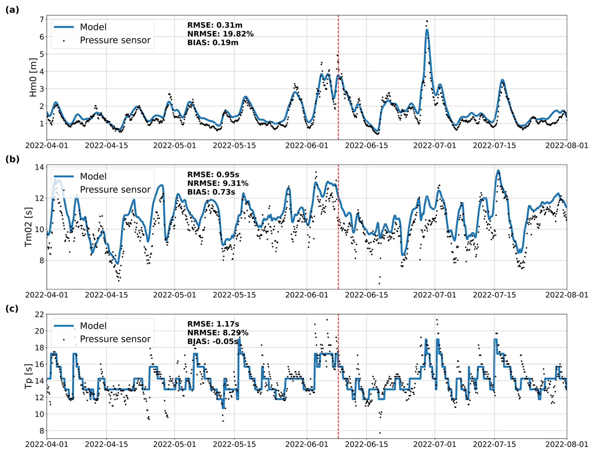
Figure 7 Wave bulk parameters derived from the pressure sensor against the model for April to August 2022 at Hermitage (Réunion) for (a) H_m0, (b) T_m02 and (c) T_p. The red line corresponds to a particular time where the power spectral density (PSD) is compared in the discussion.

3.2.2 Hawai′i

Figure 8 shows the comparison between model and wave buoy data in Hawai′i (200 m water depth) for H_m0 and T_p. The general temporal evolution of the wave bulk parameters is correctly represented, with H_m0 and T_p NRMSEs of 15.82 % and 12.99 %, respectively. However, the peaks in H_m0 tend to be underestimated by up to 1 m (see the event on 20 December in Fig. 8). The discrepancies between the modeled and observed T_p are generally related to quick shifts under multi-modal sea states, i.e., from DSS (T_p ranging from 10 to 17 s) to local wind sea (T_p ranging from 5 to 8 s) or vice versa.

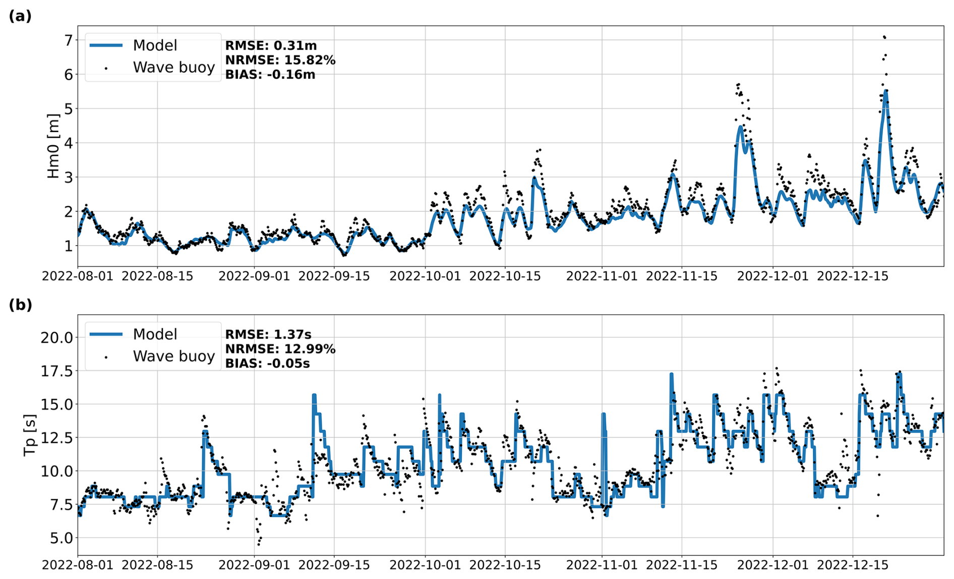
Figure 8 Wave bulk parameters estimated from the wave buoy against the model for August to December 2022 at Kauai (Hawai′i) for (a) H_m0 and (b) T_p.

3.2.3 Guadeloupe

Figure 9 depicts the comparison between model and wave buoy data at Pointe de la Grande Vigie to the north of Guadeloupe (90 m water depth) in the Caribbean Sea for H_m0, T_m02 and T_p. This figure reveals very good behavior of the model with NRMSE under 12 % for the wave bulk parameters. The strongest DSS event over the observed period (March to July 2008) is correctly captured in terms of wave periods, but the maximal H_m0 peak is again underestimated by up to 1 m. This problem is further discussed in this paper.

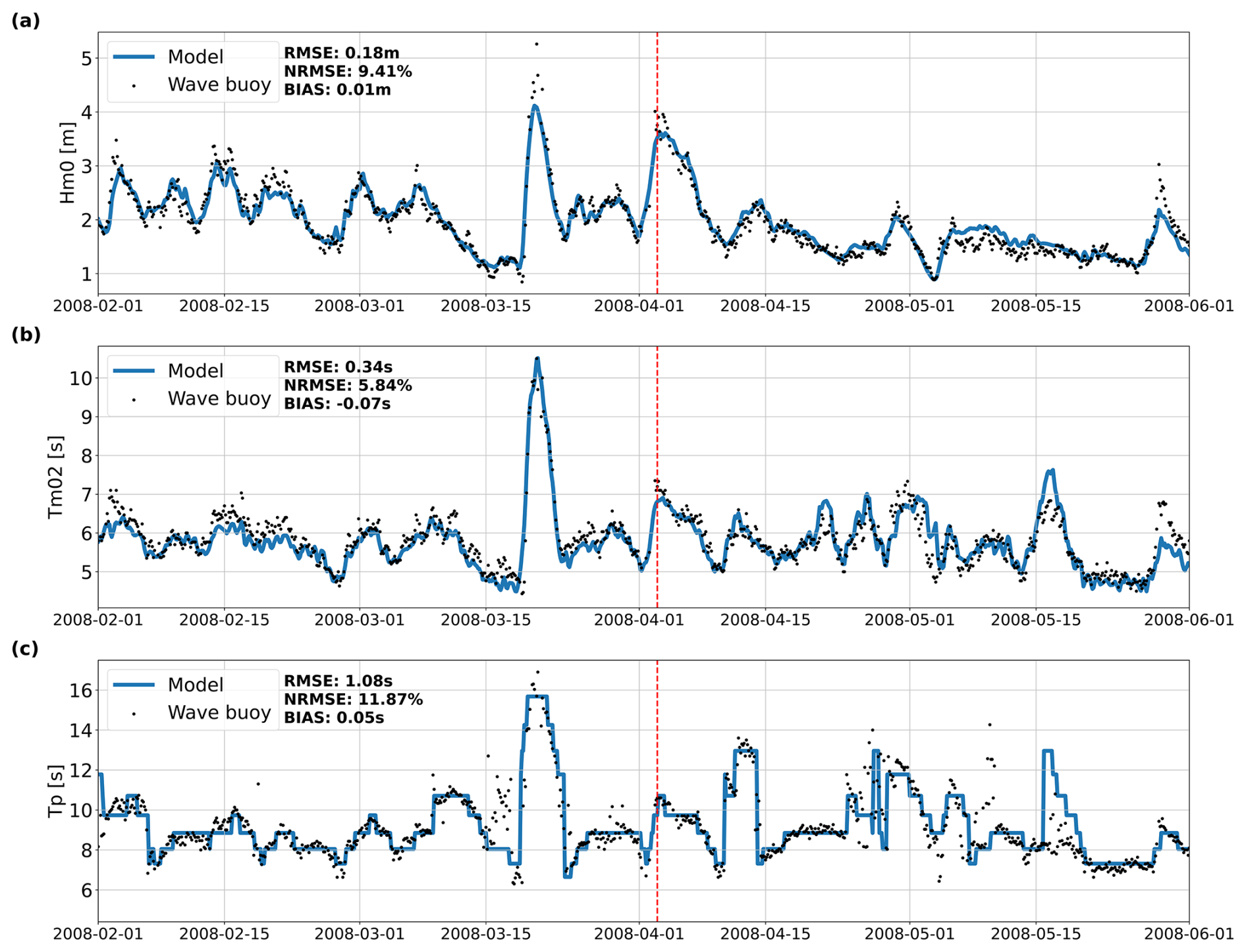
Figure 9 Wave bulk parameters derived from the wave buoy against the model for March to July 2008 at La Pointe de la Grande Vigie (Guadeloupe) for (a) H_m0, (b) T_m02 and (c) T_p. The red line corresponds to a particular time where the PSD is compared in the discussion.

3.2.4 New Caledonia

Figure 10 displays the comparison between the model and the wave bulk computed from the pressure sensor data at Nouméa (11 m water depth) for H_m0, T_m02 and T_p. The NRMSE and bias for H_m0 are 16.75 % and 0.07 m, respectively. The periods are also correctly represented with NRMSE values of 7.92 % and 14.09 % for T_m02 and T_p, respectively. Similar to Kauai, rapid fluctuations in multi-modal sea states are difficult to represent in the model and result in a higher error in T_p. More specifically, the peak of H_m0 exceeding 4.5 m on 15 March 2020 is associated with the category 1 to 2 cyclone Gretel, which passed about 150 km to the southwest of New Caledonia. This event is accurately reproduced by the model, which suggests that the sea states associated with tropical cyclones can also be accurately simulated by our model.

4 Discussion

4.1 Predictive skills and comparisons to existing global hindcasts

Focusing first on the sole wind correction by the quantile–quantile approach, better H_m0 predictions are obtained compared to the results obtained with the wind correction and source term of Alday et al. (2021). The approach presented in this study reduces the positive bias present for calmer conditions and consequently improves the general wave representation. In more detail, as seen in Fig. 6, the uncorrected SG has a lower absolute bias than either of the ERA5_QC parameterizations for the 10–12 m wave bins. Such large waves are driven by extreme winds (i.e., larger than 25–30 m s⁻¹), for which we have a limited number of observations, as can be seen in Fig. 3. Therefore, the quantile–quantile wind correction could be further improved for very high winds, provided more observations are available.

It should be mentioned that the comparison was performed using the same wind correction and source term as T475, but the whole configuration of the model presented in Alday et al. (2021) also included a multigrid approach, improved ice forcing and ocean current forcing. In our configuration, one single structured grid is used with standard ice forcing and no current effect. One can expect better results combining the comprehensive configuration of Alday et al. (2021) with our wind correction.

Existing hindcasts such as ERA5 can result in poor predictive skills when compared with coastal measurements (Samou et al., 2023). Similarly, coastal comparisons of the existing hindcasts ERA5-I and CFRS-W are limited by their global resolution of 0.3 and 0.5°, respectively (Stopa and Cheung, 2014). Global unstructured grid models emerged recently (Brus et al., 2021; Mentaschi et al., 2023), which avoid the use of the obstruction masks required for regular grids. However, the resolution employed in these studies also remains too coarse to allow for a direct validation in nearshore shallow depths. A few studies have already compared global wave models with stations located at 10–30 m water depth, although these wave buoys were moored at gently sloping inner shelves or in big lakes (Zheng et al., 2016; Alday et al., 2021). The novelty here is that, due to the steep slopes usually surrounding volcanic islands where our stations are located, such water depths are found very close to shore, typically a few hundred meters away. Specifically designed to simulate sea states around tropical islands, our new model is able to explicitly represent small islands and reach a local resolution, allowing a direct comparison with nearshore observations and a correct representation of wave transformation from deep to shallow water. Even multigrid systems, such as the ones described by Rascle and Ardhuin (2013) refined at 3^′ resolution, or more recently Dutheil et al. (2020) and Alday et al. (2021), both refined at 0.05°, are too coarse to make a direct comparison with coastal observations, often located only a few hundred meters from the coast.

4.2 Remaining challenges in deep water

However, despite these advances, areas such as polar regions, semi-enclosed seas, the Mozambique Channel and the inner seas of Indonesia, display larger errors compared to the other ocean basins (Fig. 5). In polar regions such as the Antarctic, overestimated H_m0 is likely related to inaccuracies in the representation of sea-ice dissipation, despite efforts to include icebergs (improvement of the NRMSE of 0.1 % when the icebergs were added in the present model). The sea-ice concentration in ERA5 remains uncertain, especially in the marginal ice zone (MIZ) (Renfrew et al., 2021). The oversimplified parameterization of wave propagation within sea-ice areas does not take into account the calving and drifting of icebergs into the Southern Ocean, which cause significant blocking of the wave energy (Ardhuin et al., 2011; Khan et al., 2021). Moreover, the altimetry data used for model assessment can suffer from inaccuracies in the presence of ice (Dodet et al., 2020).

Around coastlines and in semi-enclosed seas, model errors can result from wind inaccuracies associated with the land–sea transition (Xie et al., 2001; Chelton et al., 2004). In addition, ERA5 wind is known to be less accurate in mountainous areas such as in the Mediterranean Sea, where the steep orography is misrepresented by the limited resolution of the reanalysis (Graf et al., 2019; Dörenkämper et al., 2020; Gutiérrez et al., 2024). Moreover, the spatial resolution and the representation of the strongest winds may limit our ability to accurately model hurricanes (Jullien et al., 2024), although model data comparison during Cyclone Gretel off Nouméa (Fig. 10) suggests that the associated sea states can be accurately simulated a few hundred kilometers away from the cyclone eye. In the Mozambique Channel, the higher errors are probably due to the fact that currents are not represented in our model. Indeed, the strong Agulhas Current has a direct influence on the wave field propagation (Ardhuin et al., 2017). Similarly, in the Southern Ocean, accounting for the circumpolar current is known to significantly reduce the positive bias of the modeled wave height (Rapizo et al., 2018). Although currents are known to improve the model results (Marechal and Ardhuin, 2021), one of the main priorities was to produce a hindcast consistent over time. Considering that CMEMS-GlobCurrent surface currents are only available from 1993, it was decided to neglect currents in the model.

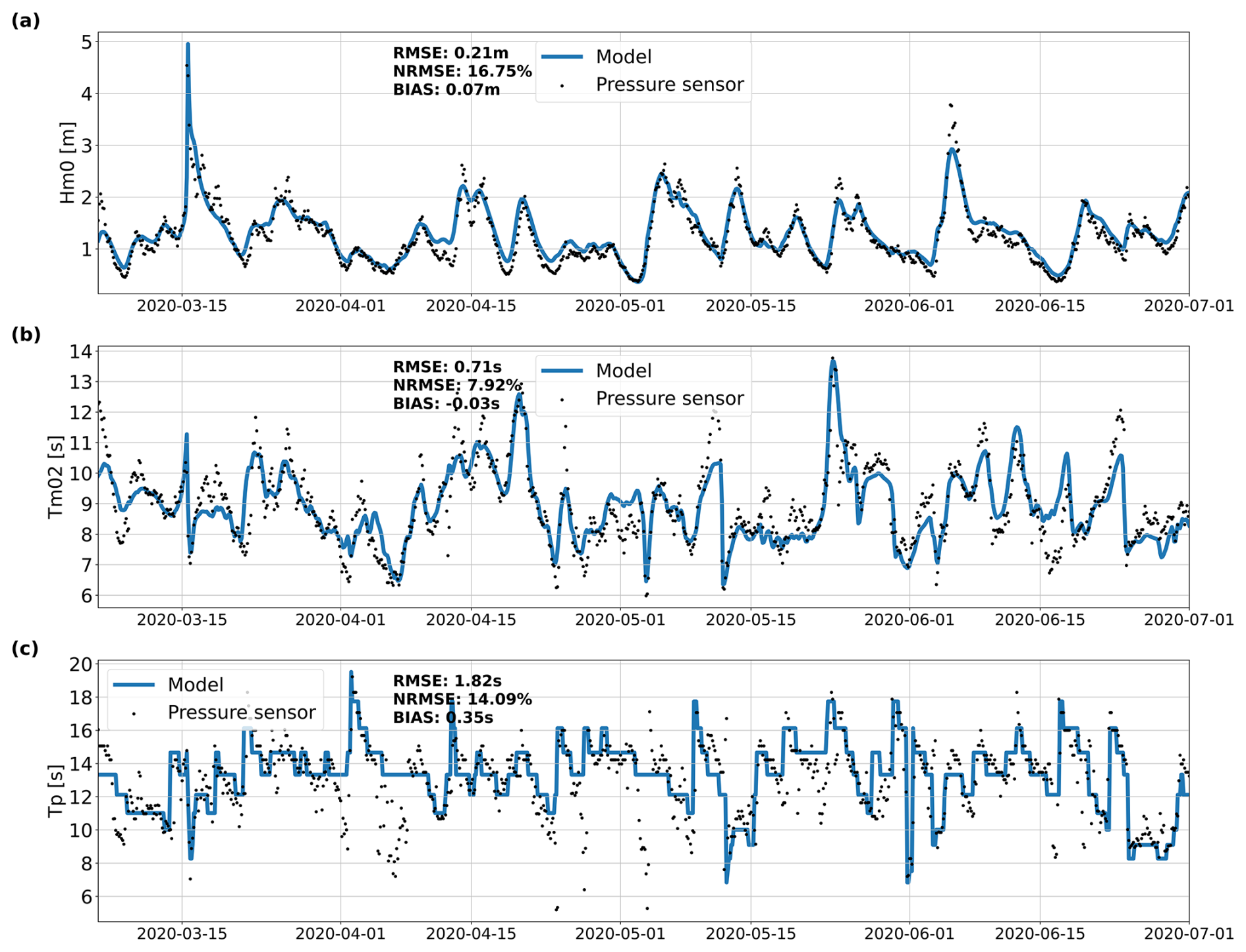
Figure 10 Wave bulk parameters estimated from pressure sensor against the model for 2020 at Nouméa (New Caledonia) for (a) H_m0, (b) T_m02 and (c) T_p.

Although the explicit representation of islands whose areas are larger than 10 km² in our UG considerably improves wave predictions in archipelago grids compared to obstruction grids, this threshold remains arbitrary. One can wonder if representing smaller islands could further improve the predictions, namely in areas with tens of thousands of islands such as Indonesia. A possible alternative would be to combine the present approach with obstruction grids for the smallest islands, following, for instance, the method of Mentaschi et al. (2018).

Keeping in mind these limitations, the present approach based on implicit schemes remains an efficient compromise between simulating the generation and propagation of sea states down to nearshore regions and maintaining a low computational cost. Modeling the sea states at a global scale with fine refinement at coastal scales is hardly practical with explicit schemes, as simulating 1 year with 200 cores takes over 50 h. The simulation presented in this study was only possible thanks to the use of implicit schemes, which overcomes the CFL constraint and therefore considerably reduces the simulation time (Abdolali et al., 2020). Indeed, for the same computational resources, a 1-year simulation with an implicit scheme took 12 h. At the wave event scale, the H_m0 peaks tend to be underestimated at some locations for the most energetic events. In order to investigate if this problem is already present in the deep ocean, Fig. 11 provides a comparison during the major 2007 DSS event between UG implicit and SG explicit results and data deduced from satellite altimetry. This comparison reveals a diffusion behavior of the UG run with an underestimation of the peak up to 0.7 m. Indeed, a possible explanation for the underestimation of the peaks of H_m0 can be the diffusion of the implicit schemes used for the UG (Roland and Ardhuin, 2014; Abdolali et al., 2020).

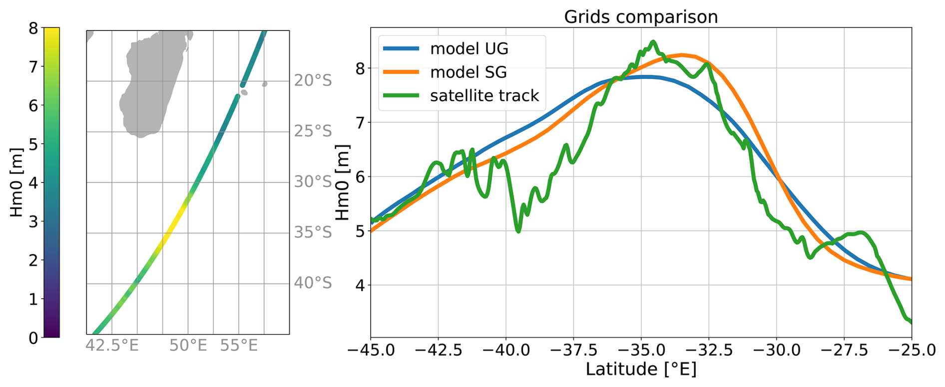
Figure 11 Comparisons between altimetry and modeled H_m0 WW3 numerical schemes at 25° S, 52° E during the major DSS on 13 May 2007.

So far, the latest version of WW3 with implicit schemes was only tested and validated for hurricanes (Abdolali et al., 2020, 2022) with short fetches and a relatively small propagation area compared to the DSS example considered here. Further research efforts are therefore required to develop new higher-order implicit schemes able to reduce diffusion and better capture H_m0 peaks. A second-order implicit scheme must remain positive and monotonous, even at high CFL numbers, which is inevitable when increasing the resolution along the coasts. For example, the Crank–Nicolson time discretization maintains monotonicity only up to a CFL number of 2. Beyond this, achieving positivity and monotonicity becomes challenging because, according to the Godunov theorem, the scheme must be nonlinear.

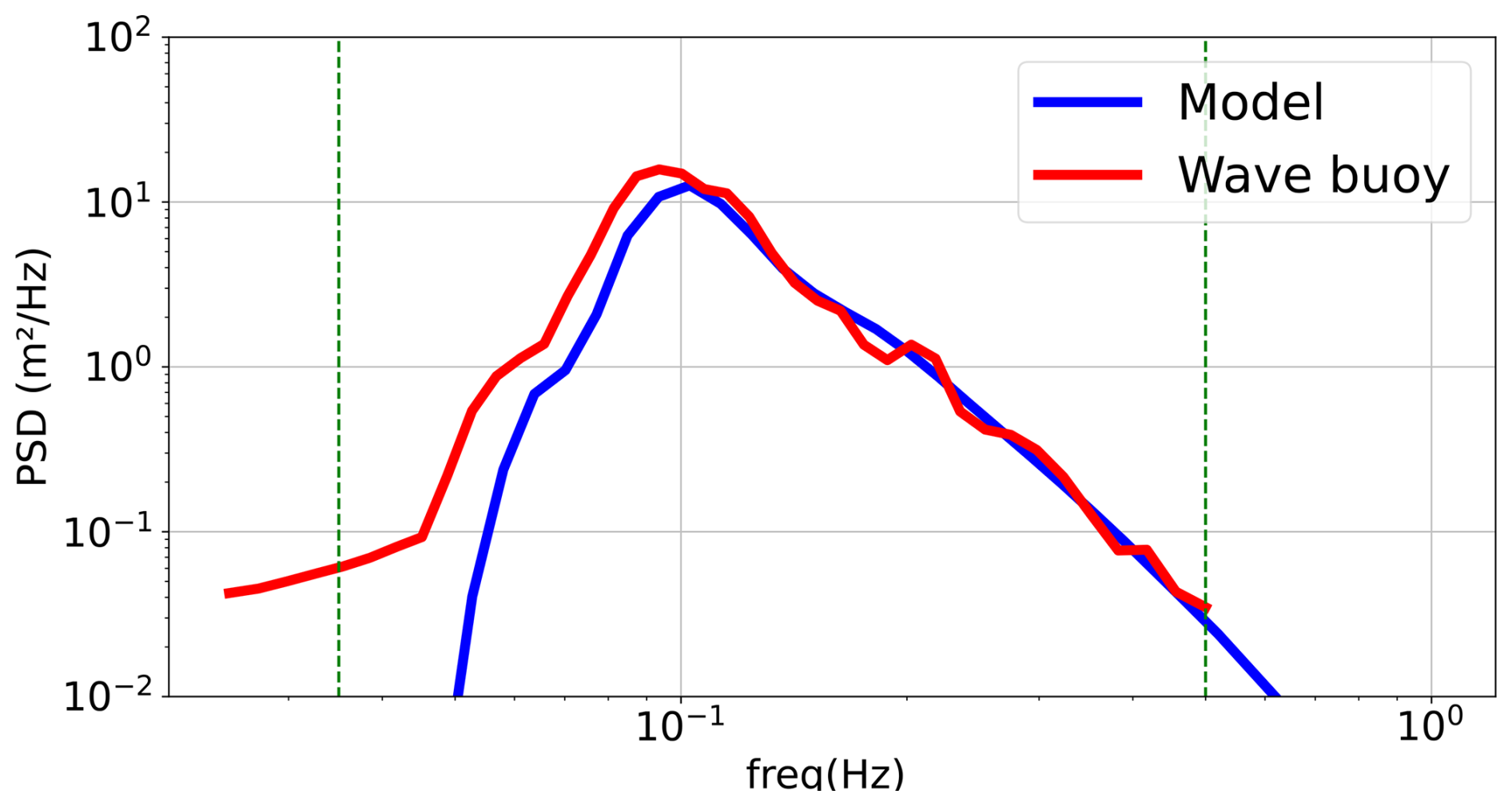
Figure 12 Comparison between modeled and observed power spectral density at 18:00 UTC on 2 April 2008 (Pointe de la Grande Vigie, Guadeloupe).

In order to further investigate the discrepancies observed, a comparison between modeled and observed power spectral density is shown at Pointe de la Grande Vigie (see Fig. 12).

This comparison shows an underestimation of the wave energy spectrum between 0.04 Hz and the peak frequency. This underestimation can be due to the parameterization of the nonlinear quadruplet wave interactions, which uses the discrete interaction approximation (DIA) of Hasselmann et al. (1985). Although widely used, the DIA is a crude approximation, as shown by Benoit (2007), van Vledder et al. (2012), and Alday and Ardhuin (2023). Other alternative methods exist (Webb, 1978; Tracy and Resio, 1982; Hasselmann and Hasselmann, 1985; Masuda, 1980) but require very high computational costs and are therefore not practical with a global model. The underestimation of the wave energy spectrum below 0.04 Hz is discussed in the next section.

4.3 Remaining challenges in coastal water

At a global scale, the comparison between altimeter data and modeled H_m0 results in a NRMSE of 11.6 %. In coastal zones, the comparison against in situ data shows H_m0 NRMSE values between 9 % and 22 %, i.e., generally consistent with the error observed in surrounding deep waters. Very close to shore and in shallow depths (Réunion and New Caledonia), the model also shows comparable predictive skills, which demonstrates that the wave transformations from deep to shallow water are correctly simulated, despite the challenges associated with the presence of steep slopes. Both modeled wave periods T_m02 and T_p display similar accuracy to that of H_m0 (NRMSE values <20 %), although T_p remains more unstable under multi-modal sea states.

In coastal zones, the underestimation of the energy spectrum below 0.04 Hz that can be seen in Figs. 14 and 12 can be attributed to the presence of infragravity waves (see Bertin et al., 2018, for a recent review), which are not represented in the present model. At Grande Vigie station (Fig. 12), the 90 m water depth implies that energy in the IG wave band corresponds to free IG waves reflected along the coast, a problem discussed by Alday et al. (2021). Part of the discrepancies closest to shore can be attributed to the finest mesh resolution of 100 m (Fig. 13). Even though it is a very high refinement for a global model, it remains too crude to represent the rapidly varying bathymetry related to the complex reef (Buckley et al., 2016). In order to make clear recommendations concerning the minimum resolution required for such comparisons, we need more adequate measurements, and we await forthcoming high-resolution simulations to carry out comparative studies. Additionally, the issue of resolution remains closely tied to interpolation issues when comparing measurements and models in rapidly varying media.

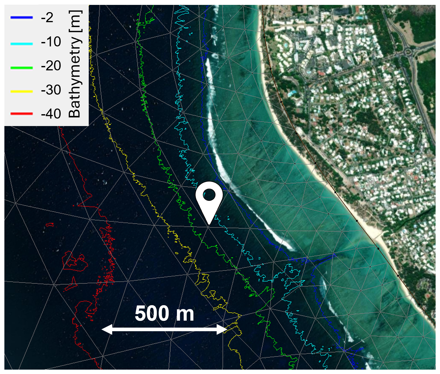
Figure 13 Satellite view of the Hermitage fringing reef (Réunion) with the extension of the model grid, a detailed bathymetry map (extracted from Litto3D lidar data (IGN and SHOM)) and the location of the pressure sensor on the reef.

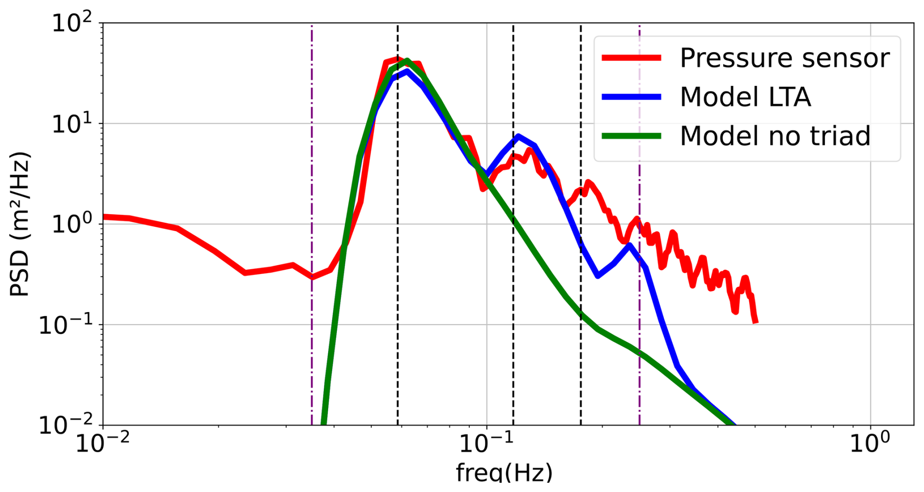
Figure 14 Comparison between power spectral density derived from pressure measurements (red) and modeled with (blue) and without (green) triads at 09:00 UTC on 8 June 2022 (Hermitage, Réunion). The purple lines represent the cut-off frequencies. The black lines represent the peak frequency and the superharmonic frequencies.

The steep bathymetries usually bordering tropical islands (with bottom slopes locally easily exceeding 1:10) pose an additional challenge to spectral models. Indeed, spectral models are based on the wave action equation, which was derived for waves propagating in “slowly varying media” (Bretherton et al., 1968), a condition that is not met for such steep slopes.

When the waves approach the coast, triad interactions transfer energy from the peak frequency to lower (subharmonics) and higher (superharmonic) frequencies. In this model, the lumped triad approximation (LTA) of Eldeberky (1996) is used to reproduce the energy transfer towards higher frequencies. Although widely used, the LTA is a crude approximation and can only represent the second harmonic, which can result in high energy differences at high frequencies, as seen in Fig. 14. Since the mean period T_m02 is sensitive to high frequencies, this problem could explain why we have higher errors in this parameter in shallow depths (as seen in Fig. 7).

5 Conclusions

A new global high-resolution wave model for the tropical ocean is presented in this paper. The model aims at better simulating the sea state in the tropical ocean, which requires capturing the large extent of DSS propagation (i.e., global model) while having a high local refinement to explicitly represent islands (i.e., high refinement). Our approach combines the use of an unstructured grid, with a global resolution of 50 km refined down to 100 m in nearshore areas of interest, and an implicit scheme, which substantially reduces computational cost. In addition, we develop a new quantile–quantile correction for ERA5 wind, resulting in small biases for most wave heights. In addition to classic validation in deep waters against satellite altimetry data, this modeling strategy allows us to perform for the first time direct comparisons in shallow depths that are very close to shore due to the steep slopes usually surrounding tropical islands.

Despite difficulties related to the possible diffusion of the implicit scheme and the representation of nonlinear interactions, the model gives promising results with a correct representation of the wave transformation, from deep to shallow water. The availability of long-term in situ data remains one of the main challenges in validating wave models in tropical volcanic islands. The lack of wave measurements is usually due to a combination of remote location, difficult access, very steep seabed slopes and strong exposure to waves, which makes deployment in shallow areas even more challenging. The availability of spectrum data is particularly helpful in understanding the origins of possible discrepancies between the model and observations. In addition to the need to pursue the deployment of local in situ surveys, new satellite data, such as the recently launched Surface Water and Ocean Topography (SWOT) mission, should provide useful high-resolution wave measurements close to shore (Chelton et al., 2022) and facilitate validation of global and coastal models.