The unicellular NUM v.0.91: a trait-based plankton model evaluated in two contrasting biogeographic provinces

Trait-based models founded on biophysical principles are becoming popular in planktonic ecological modeling, and justifiably so. They allow for slim, efficient models with a significant reduction in parameters that are well-suited to modeling past and future climate changes. In their idealized forms, trait-based models describe the ecosystem in one set of parameters defined by first principles and rooted in physics, chemistry, geometry, and evolution. The result is an emerging ecosystem defined by physical and chemical limitations at the cell level. At present, however, a significant part of these parameters is not fully constrained, which potentially introduces considerable uncertainty into the model results. Here, we investigate how these parameters influence the ecosystem structure of one of the simplest trait-based models, the Nutrient-Unicellular-Multicellular (NUM) model. We describe the unicellular module of the NUM model and, through an extensive parameter sensitivity analysis, we demonstrate that the model – with a large span in parameters – can capture the general features of the picoplanktonic, nanoplanktonic, and microplanktonic ecosystem in a high-productivity upwelling system. We demonstrate that it is possible to narrow the range of parameters to get a stable and acceptable solution. Finally, the model responds correctly in an oligotrophic downwelling system using parameters fitted to the upwelling system. Our analysis demonstrates that the unicellular module of the NUM model is broadly accessible without detailed knowledge of the parameter settings and that the first-principles approach is well-suited to modeling poorly resolved regions and ecosystem evolution during current and deep-time climate change.

1 Introduction

Trait-based models are becoming an important tool for understanding the spatial and temporal pattern of the planktonic ecosystem structure (e.g., Follows et al., 2007; Dutkiewicz et al., 2021; Ward et al., 2019; Eckford-Soper et al., 2022). Rooted in first principles of biophysics and biochemistry, trait-based models alleviate many of the caveats that confine traditional functional planktonic ecosystem models: they allow for large-scale ocean domains without the need to add increased complexity, they reduce the amount of parameter tuning, and they allow for modeling of evolution in the past and future under climate change where ecosystems were different from the ones we know today (Reinhard et al., 2020; Sauterey et al., 2017; Wilson et al., 2018; Archibald et al., 2022).

There are a variety of approaches to trait-based modeling. For most of the trait-based plankton ecosystem models, size is used as a master trait, as it scales with many of the cell processes and rates (Ward et al., 2019; Sauterey et al., 2015; Andersen et al., 2015). One particularly simple size-based plankton model is the Nutrient-Unicellular-Multicellular (NUM) model (Andersen and Visser, 2023; Serra-Pompei et al., 2020; Serra-Pompei et al., 2022). The NUM model is founded on the biophysical and chemical processes of the cell scaled up to the community level (Fig. 1). With the cell processes at the center, the result is a simple and fast model where the size spectrum, rates of photosynthesis, and uptakes of nutrients, dissolved organic carbon (DOC), and food (phagotrophy) emerge from the specific physical conditions of the oceanographic conditions (Andersen and Visser, 2023; Serra-Pompei et al., 2020).

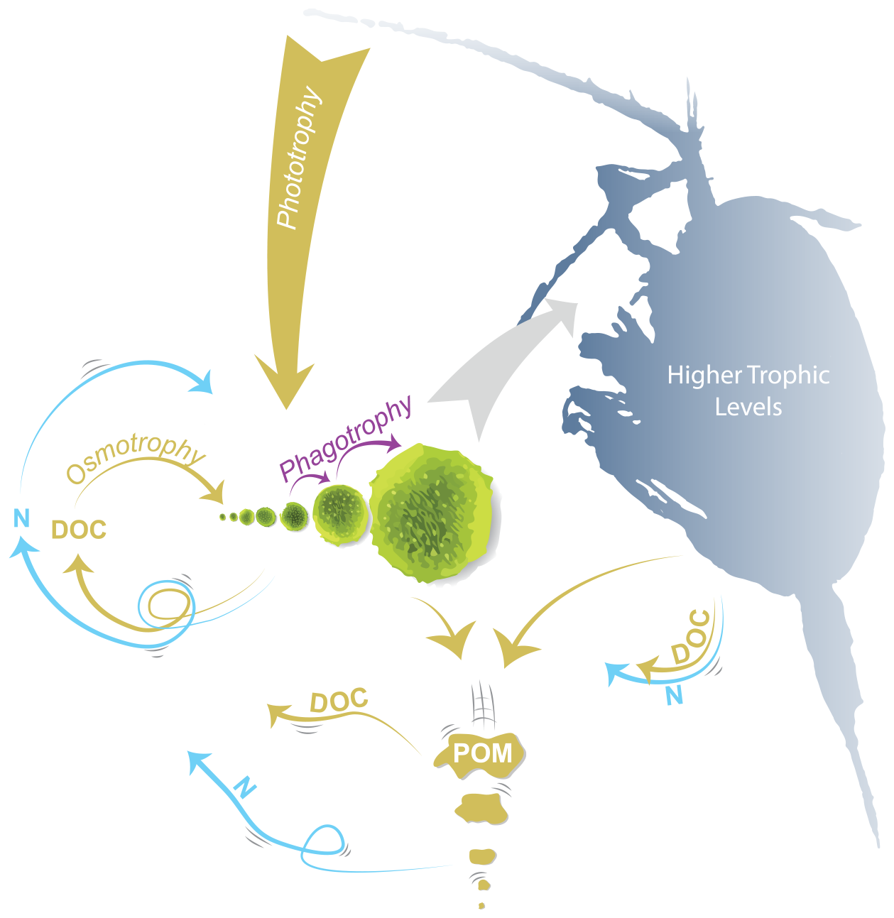
Figure 1 Schematic of the unicellular module of the Nutrient-Unicellular-Multicellular (NUM) model. The unicellular organisms are represented here by seven size classes of organisms that can all get their nutrients and carbon from osmotrophy, phototrophy, and phagotrophy. The uptake rates depend on the biophysics of the cell and the environmental availability of dissolved organic carbon (DOC), nutrients (N), light, and food (smaller cells). Higher trophic levels are parameterized here as feeding on a specific size range of cells. Exudation, viral lysis, assimilation losses, and higher trophic level losses replenish the nutrients and carbon. Losses from sloppy feeding by phagotrophy and higher trophic levels are reintroduced as particulate organic matter (POM) that sinks down through the water column and is remineralized into DOC and N. The model formulations are listed in Sect. S1.

Despite the simplicity of the NUM model, it – like any other model – relies on a set of parameters (Table 1). In principle, these parameters are universal and common to all organisms; however, they are not all well-established. Some parameters are well-defined by cell physiology, e.g., the maximum diffusive nutrient affinity coefficient (α_D) that is limited by cell surface area, but many have a range of uncertainty that emerges from natural cell variability or from a limited understanding of a parameter. As with any model, the output of the NUM model reflects the parameter choices. It is still, however, unclear how much the parameters influence the result, how much tuning the model requires, and how well the model transfers between sites with the current parameter uncertainty.

Table 1 Parameters used in this study. The reference values are based on arguments from Andersen and Visser (2023) and the standard values used in the NUM model setup.

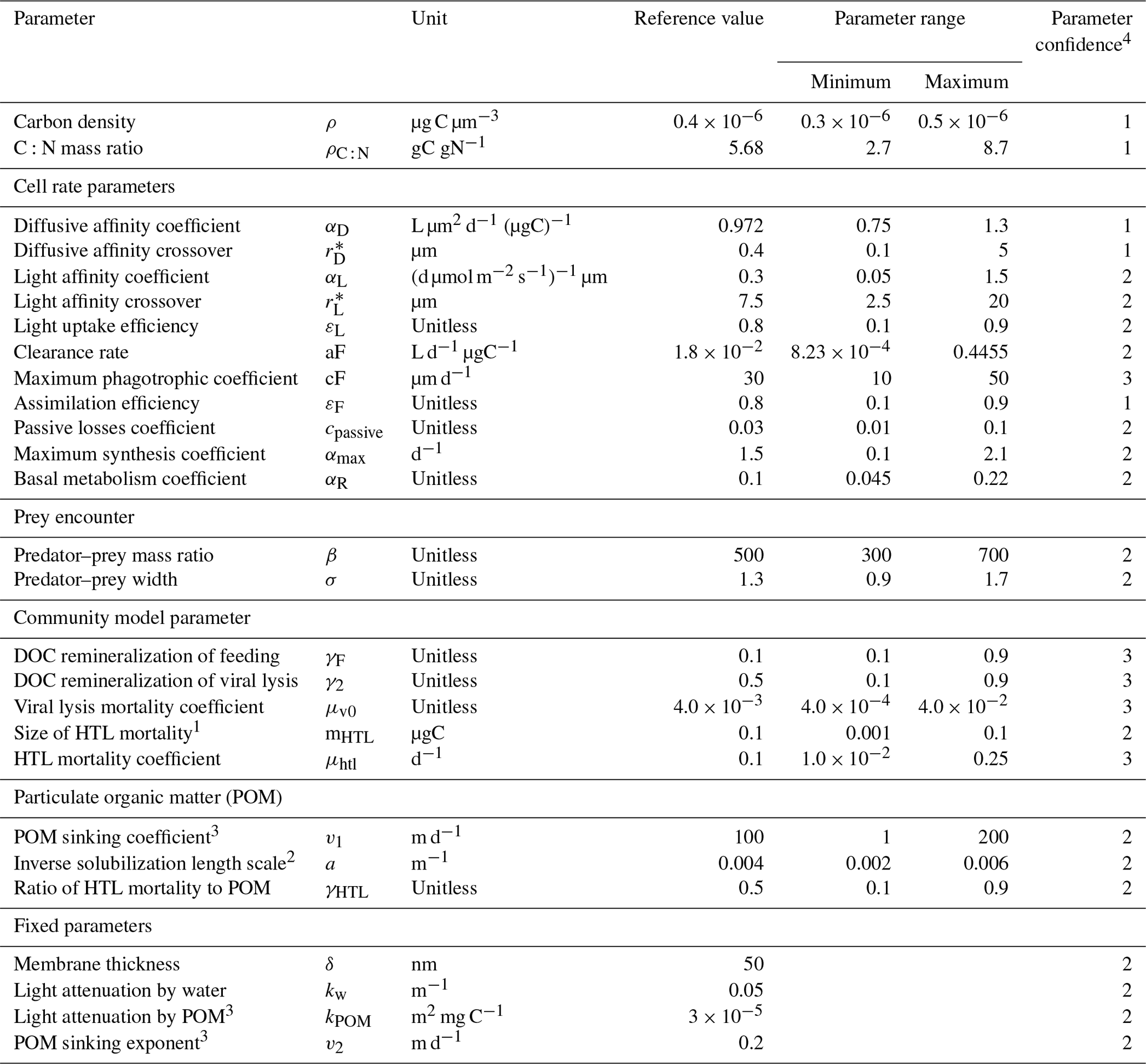
¹ The HTL mortality is between 100 and 10000 times smaller than the largest cell size. ² Fennel et al. (2001). ³ POM was not included in previous versions of the NUM model, and the parameters written in the reference value signify the values used in the initial evaluation of the model. Based on arguments in Sect. S1, a k_POM value of 3 × 10⁻⁵ m² mg C⁻¹ is used for all the simulations in this article. The choices of POM sinking coefficient and exponent result in sinking speeds of 0.01–3 m d⁻¹ for the smallest POM size classes and 1–200 m d⁻¹ for the largest ones using the formulation for POM sinking in Sect. S1. ⁴ Qualitative parameter uncertainty ranging from 1 (low) to 3 (high) (Andersen and Visser, 2023). The parameter uncertainty stems from limited understanding of the processes and/or empirical evidence.

In this article, we describe the unicellular module of the NUM model and evaluate the model's ability to capture well-established key ecosystem descriptors, its robustness, its geographical transferability, and the relative importance of the underlying parameters. Specifically, we start by evaluating the model's ability to capture the size structure of the planktonic biomass of the California Current Ecosystem (CCE) (California-Current-Ecosystem-LTER and Landry, 2019; Taylor and Landry, 2018) using the default model parameters. Hereafter we evaluate how the parameter uncertainty affects the model sensitivity. We conclude by applying the identified optimal parameter values for the CCE to station ALOHA north of Oahu, Hawaii, in a test of the model's geographical transferability (Pasulka et al., 2013; Taylor and Landry, 2018).

2 Model description

2.1 The Nutrient-Unicellular-Multicellular model framework

The NUM model is built on an additive model framework that relies on formulations of the fundamental properties of the organism (Andersen and Visser, 2023; Serra-Pompei et al., 2020; Serra-Pompei et al., 2022). The NUM model initially included copepods and protists as the unicellular and multicellular components, along with nutrient (N) and fecal pellets (Serra-Pompei et al., 2020). Serra-Pompei et al. (2020) implemented the model in MATLAB with a chemostat setup. Later, Serra-Pompei et al. (2022) coupled the NUM model to a transport matrix, enabling both water column and global simulations. A major update of the NUM model resulted in the current version where the core NUM model was translated from MATLAB to FORTRAN95. The model can be run directly from FORTRAN but can also be initialized from MATLAB and R, which makes the model accessible to users without FORTRAN experience. In this update, the NUM framework was extended to include a DOC module and a particulate organic carbon (POM) module.

The NUM model can be used in three different setups. It can be used in a global simulation where it is coupled to a transport matrix that provides the advection, diffusion, and temperature for the simulation (Khatiwala, 2007). It can be used in a chemostat setup with a constant mixing rate and deep nutrient concentration. Finally, as we do here, it can be used in a water column simulation where the temperature and diffusion at a single location are extracted from the transport matrix. Here, we describe and evaluate the unicellular organisms and the particulate matter, and we will therefore limit the description of the NUM framework to these parts. The model formulations are provided in Sect. S1 in the Supplement. Section 2.2 describes the unicellular module and parameters, while Sect. 2.3 describes the new simple DOC and POM modules and the associated parameters.

2.2 The unicellular module

The backbone of the NUM model is the unicellular module that comprises the classic functional groups of phytoplankton, osmotrophic bacteria, and zooplankton. While unicellular organisms span many orders of magnitude across all types of trophic strategies (feeding mechanisms), they are all described with one set of parameters in the unicellular subroutine of NUM. Here, the cell may be visualized as one type of organism – we refer to this as a generalist – that is essentially a mixotroph in the sense that it is able to perform osmotrophy (diffusive uptake of DOC), photosynthesis, and phagotrophy (food consumption) to gain nutrients and carbon. The generalist can utilize all three trophic strategies at the same time. However, the yield from each of these strategies depends on the size of the generalist and the surrounding environmental conditions (light level, nutrient and dissolved organic carbon concentration, and food). The model contains several of these generalists, with the only difference being the size of the organism, which is defined in logarithmic size bins of mass m. The output of the generalist subroutine is the biomass of each of the generalist size bins and the associated rates of phototrophy (J_auto), osmotrophy (J_osmo), and phagotrophy (J_phag). This approach makes the unicellular module especially well-adapted to handling mixotrophic organisms. In the following subsections, we will go through the most important processes controlling the generalist growth and size structure. The aim of this section is to give the reader an understanding of the mechanisms that control the organism and a sense of the parameters that are evaluated in this study. The important parameters are highlighted in bold in the text below. The following sections summarize the more detailed descriptions of the model given in Serra-Pompei et al. (2020) and Andersen and Visser (2023).

2.2.1 Resource uptake

The organism's affinity for (meaning its ability to take up) dissolved organic matter and nutrients (a_D), light (a_L), and food phagotrophy (a_F) is dependent on its size. The affinities for uptake of these resources are determined by the encounter rate (how many resources the generalist is in contact with) and the assimilation rate (how fast it can take up a resource it encounters).

The affinity for diffusive uptake of nutrients and DOC is modeled as a crossover between two size regimes: large and small organism sizes. For large organisms, the limiting factor is the rate of diffusion towards the outer cell membrane. In contrast, for smaller organisms, it is the number of cell porter channels that transport the resource across the cell membrane (Eq. 1; all equations referred to are listed in Table 2). The parameter $r_{\mathrm{D}}^{*}$ determines the organism size where the crossover between the two regimes occurs, and the diffusive affinity coefficient, α_D, defines the upper limit of the diffusive encounter.

Table 2 Equations used for the unicellular submodule. A full model description is given in Sect. S1.

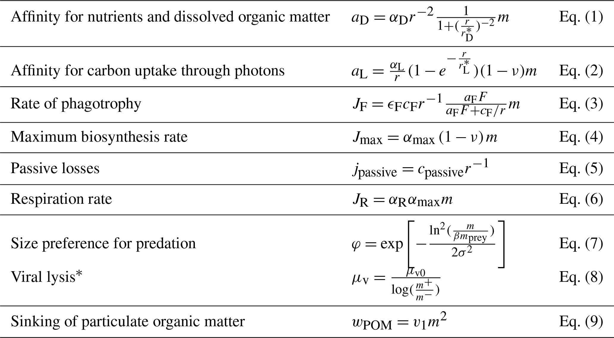
^* m⁺ and m⁻ are the masses of the upper and lower limits of the size bin.

The affinity for uptake of carbon through photosynthesis, a_L, is also modeled as a crossover between two regimes (Eq. 2). For small organisms, a_L is dependent on an organism's mass, while for larger organisms, where light-harvesting complexes create internal shading, a_L is dependent on the cell surface area. The parameter $r_{\mathrm{L}}^{*}$ determines the crossover size between the two regimes. The parameter α_L is defined as ${\mathit{\alpha }}_{\mathrm{L}}=\mathrm{3}y/\left(\mathrm{4}\mathit{\rho }\right)$, where y is the quantum yield (describing the efficiency of the process relative to the available photons) and ρ is the carbon density of the individual cell (Andersen and Visser, 2023). The light uptake efficiency (ε_L) is a fraction that defines how efficient the organism is at utilizing the available light.

Phagotrophy is modeled as a hyperbolic curve where the amount of prey ingested increases with the prey density until saturation of prey ingestion occurs. Such an ecological type-II functional response has a constant affinity (the clearance rate a_F) and a maximum assimilated phagotrophic uptake that are dependent on the assimilation efficiency (ε_F) and the maximum phagotrophic coefficient (c_F) (Eq. 3).

2.2.2 Synthesis, respiration, and losses

The generalist might be able to take up more nutrient and carbon than it is able to synthesize. The rate of biosynthesis is controlled by the maximum synthesis coefficient (α_max, Eq. 4). Nutrients and excess carbon leak out of the cell. Besides the resource uptake, the organism passively leaks carbon and nutrients through the cell membrane. This process is modeled as a constant, c_passive, divided by the radius of the organism (Eq. 5). Finally, the organism's respiration rate is modeled as a fraction of the maximum synthesis coefficient (Eq. 6). This is called the basal metabolism coefficient, α_R.

2.2.3 Prey–predator interactions

The generalist is potential prey for two groups: other larger generalists and predators from higher trophic levels. The generalist's internal prey–predator relationship is based on the two parameters β and σ (Eq. 7). B defines the mean mass ratio between the prey and the predator. The parameter σ defines the wideness of the preferred size range that a predator preys on. The mortality from higher trophic levels is likewise defined by two parameters, i.e., m_HTL, which defines the lower limit (expressed as mass) of organisms that are preyed on by higher trophic levels, and the higher trophic level mortality coefficient, μ_HTL, which defines the rate of predation by higher trophic levels. Lastly, the generalists undergo viral lysis. The rate is controlled by the parameter μ_v0 and is dependent on the logarithmic size bin length (Eq. 8)

2.3 Dissolved organic carbon and particulate organic matter

This version of NUM incorporates both dissolved and particulate matter into a simplified approach (Fig. 1). Dissolved nutrients, both containing inorganic and organic N, are modeled as one dissolved N pool, while DOC is modeled separately. The POM contains both C and N in a fixed ratio. Dead cells, feeding losses, and higher trophic level mortality produce both POM and dissolved constituents (DOC and N). Note that the choice of pooling inorganic and organic N in a single pool means that the microbial consumption and remineralization of N are not explicitly resolved as being dependent on osmotrophy. In contrast, consumption of DOC as an energy source for heterotrophic osmotrophy is explicitly modeled as presented above (Sect. 2.2.1). The pool of DOC in this model represents “labile” DOC. The divisions between the particulate and dissolved fractions are determined by the γ parameters (γ₂, γ_F, and γ_HTL), which describe how much of each flux (mortality, feeding losses, and higher trophic level mortality) is routed to the dissolved fractions, with the remaining losses transferred to POM. Particulate organic matter is divided here into two different size fractions (a number that can readily be increased in future applications). POM derived from dead cells and feeding losses is transferred to the largest POM size fraction, which is smaller than the size of the original cell. POM from higher trophic level mortality is transferred to the largest POM size fraction. POM sinks with a size-dependent velocity, which is described as a power function with parameter v₁ and exponent v₂ (Eq. 9). POM is assumed to remineralize directly to the dissolved N and DOC pools. This process of remineralization is not explicitly microbial-cell-related in the model but occurs at a constant rate determined by the inverse of the solubilization length scale (a) as rem_POM=aw_POM. The model formulation of nutrients and the DOC and POM modules are given in Sect. S1.

3 Modeling approach

In this article, we use the water column setup of the NUM model to simulate the conditions at the southern CCE and station ALOHA. We initially perform a general validation of the model with default parameters against the mean biomass size spectrum and nutrient profile for the two locations. The subsequent analysis is aimed at understanding the model's performance, robustness, transferability, and parameter sensitivity.

The investigation has two levels: an overall broad random parameter evaluation followed by three more detailed statistical sub-analyses. The first-level parameter study is comprised of 100 000 simulations with quasi-random input parameters in the range defined in Table 1. Of the 23 free parameters, several are assigned a span of several orders of magnitude, which is computationally demanding but enables a genuine investigation of the solution space and variability for the model. We use a Latin hypercube sampling scheme for all 23 parameters to ensure an even spread in the entire parameter space (McKay et al., 1979; Stein, 1987) and evaluate the model performance by comparing the results with observations, using a set of statistical matrices that will be described below. We moreover use this first-level parameter study and evaluation to identify optimized parameter combinations that result in a good model fit to the CCE observations. These optimized parameter combinations define a restricted parameter span that permits us to perform three additional statistical sub-analyses for CCE. The first sub-analysis is a set of 10 000 simulations where the input parameters are quasi-randomly sampled with the Latin hypercube sampling scheme within the restricted parameter span. This sub-analysis allows us to determine whether only a very specific combination of parameters results in a good model fit or whether the model performance is increased by simply reducing the parameter span. The second sub-analysis is a set of local sensitivity analyses where the model's sensitivity to each of the parameters is evaluated separately with the outset in an initial parameter combination (Zhou and Lin, 2008). The local sensitivity analysis is done with the outset and the initial parameter combinations that perform best for CCE. Each of the parameters is varied successively in 50 evenly distributed intervals within the restricted parameter span. This sub-analysis showed that several of the parameters result in system bifurcation points where the model solution changes abruptly. While extremely interesting, detailed analysis of such bifurcation points is beyond our current scope and remains a prospect for future analyses. The sub-analysis also showed that most parameters are highly coupled in terms of ecosystem sensitivity, where the effects of individual parameters are intertwined and result in a highly nonlinear system. The sensitivity analysis with a specific parameter outset yielded nearly equal sensitivities for almost all of the parameters, whereas, with a different parameter outset, ε_F was the absolute most important parameter. Because of these highly nonlinear parameter interactions, local sensitivity studies give little added information about model performance. We have added two of these seven tests in Sect. S4. The third sub-analysis is a global variance-based sensitivity analysis using Sobol's method and a sensitivity index (Bilal, 2014; Sobol, 1993, 2001). The global variance-based sensitivity analysis accounts not only for the effect of each individual parameter on the modeled result (the first-order effect), but also, more interestingly, the effect of a parameter through its interactions with other parameters (total effect) (Bilal, 2014; Zhou and Lin, 2008). The global sensitivity analysis is done following Bilal (2014) with a set of 20 000 simulations with parameter combinations based on random sampling of the restricted parameter span. Then, for each of the 20 000 simulations, we step through the parameters and perform two simulations: (1) the parameter in question is kept at its value while the other 22 parameters are selected quasi-randomly within the restricted parameter span, and (2) the parameter in question is randomly selected in the parameter span while all the other parameters are kept at their values (Bilal, 2014; Sobol, 2001). A step-by-step description of the process for setting up the global sensitivity analysis is included in Sect. S5.

The model evaluation and statistical test against the CCE permit us to identify seven optimized parameter combinations that result in a good model fit to observations for CCE. We then finally evaluate how the model performs within the restricted parameter spans at station ALOHA that, with its different physical and chemical conditions, represent an oligotrophic downwelling system. These results are evaluated against a first-level parameter study at ALOHA with 100 000 quasi-random parameter combinations.

3.1 Observational data

Compilations of the compositions of phytoplanktonic communities have illuminated some systematic trends in the size distribution of planktonic organisms as a function of chlorophyll and autotrophic biomass concentration (AC_bio) (Taylor and Landry, 2018; Maranon et al., 2012; Ward et al., 2014). Analyses across various provinces in the Atlantic and North Pacific broadly reveal that, when chlorophyll a (chl a) or primary production is low, ∼ 40 % of the biomass is dominated by picophytoplankton (0.2–2 µm), irrespective of temperature. As chl a increases, microphytoplankton (> 20 µm) increase in biomass and dominate when chl a is high. Nanophytoplankton (2–20 µm) are intermediate between picoplankton and microphytoplankton at both low and high chl a. Similar trends are present at the subregional or local scale in detailed work that is described below (Taylor and Landry, 2018; Taylor et al., 2015; Goericke, 2011) (Fig. 2). Because of the apparent pervasiveness of these trends and characteristics of the planktonic community in marine ecosystems, size structure represents an excellent test for the model's adaptability across oceanographic regimes.

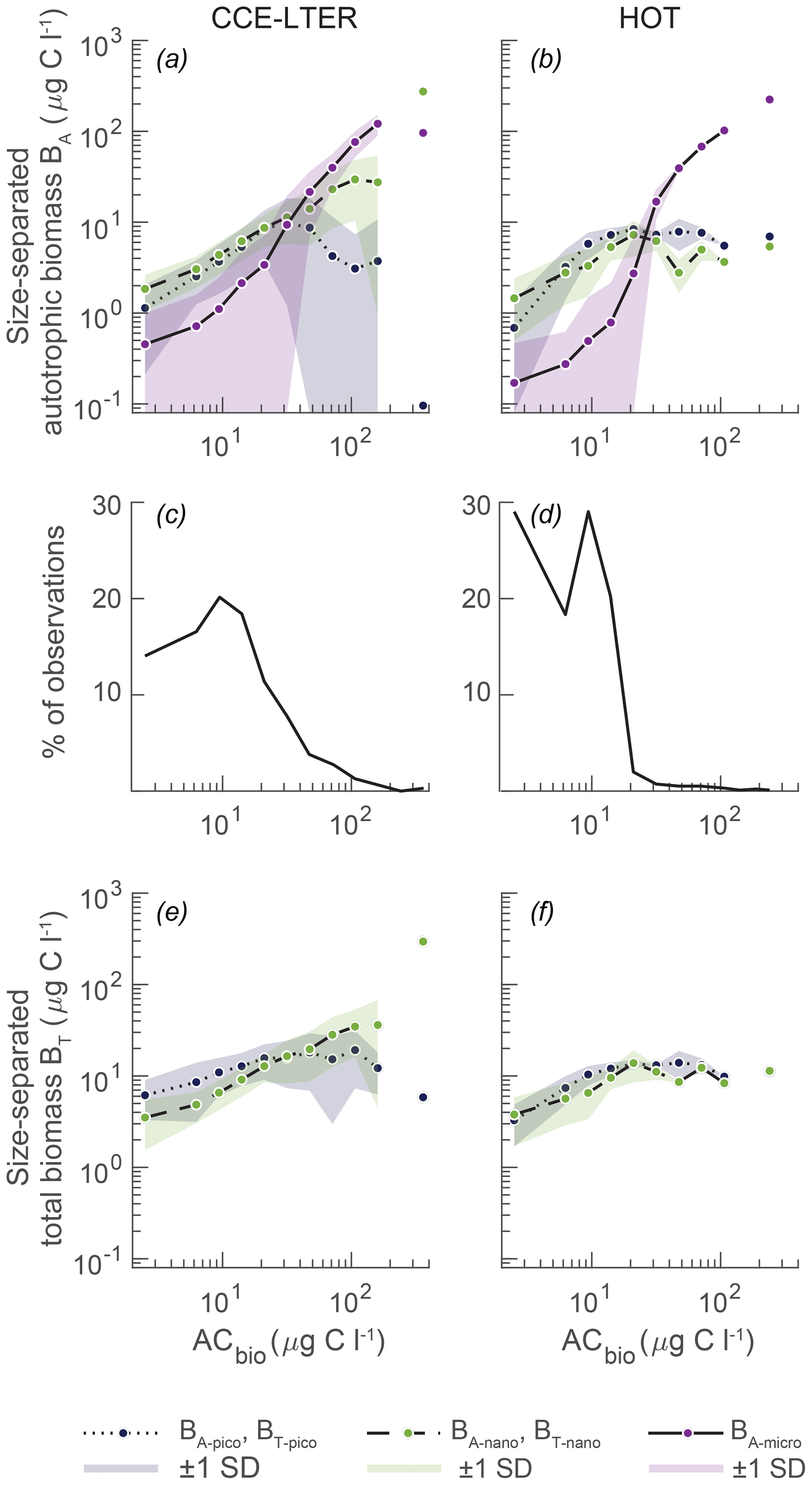
Figure 2 Observed plankton biomass as a function of total autotrophic biomass (AC_bio). (a, b) Mean biomass of picoautotrophs (< 2 µm, B_A-pico), nanoautotrophs (2–20 µm, B_A-nano), and microautotrophs (> 20 µm, B_A-micro) at (a) CCE with upwelling and (b) HOT with downwelling. The data have been compiled from depths of 0 to 200 m from 2004 to 2011 and placed in logarithmically distributed bins. (c, d) Number of observations per bin at the respective sites. (e, f) The total picoplankton (B_T-pico) and nanoplankton (B_T-nano) biomass at CCE and HOT is the sum of the autotrophic and heterotrophic biomasses. The data and binning method are from Taylor and Landry (2018) and the references in the text. Note that CCE relative to HOT is more eutrophic, which is reflected in the higher amount of data in the higher AC_bio bins (c vs. d).

Here, we compare the model result to size spectrum data gathered from the southern CCE as part of the California Current Ecosystem Long Term Ecological Research (CCE-LTER) and from station ALOHA, which is the long-term Hawaii Ocean Time (HOT) series (Taylor and Landry, 2018; Pasulka et al., 2013; California-Current-Ecosystem-LTER and Landry, 2019) (Fig. 2). These two sites reflect distinctly different oceanographic regimes: coastal upwelling with eutrophic conditions at CCE and downwelling oligotrophic open-ocean waters at station ALOHA. Both sites have been regularly sampled for epifluorescence microscopy and flow cytometry in the years 2004 to 2011, resulting in large datasets of biomass abundance, size structure, and planktonic composition. The phytoplanktonic size structures of the two sites show many of the same features as the large-scale compilations of the planktonic size distribution: picoautotrophic and nanoautotrophic organisms dominate the size spectrum at low autotrophic carbon biomass (AC_bio), where the concentrations of microautotrophic organisms are very low (Fig. 2a, b) (Taylor and Landry, 2018; Maranon et al., 2012; Ward et al., 2014). The concentrations of all three size classes increase with increasing AC_bio. However, the autotrophic microplankton concentration increases more quickly than the smaller size groups and becomes dominant at intermediate levels of AC_bio (approximately 20 µg C L⁻¹). Microautotrophic plankton continues to increase in a power law fashion for both observational datasets. In contrast, the picoautotroph and nanoautotroph increases as a function of AC_bio are different at the two sites. The CCE-LTER dataset follows the global tendency of a continued increase in nanoautotrophs, while the picoautotrophs decrease towards high AC_bio. The HOT observations show steadier concentrations for both picoautotrophs and nanoautotrophs across the AC_bio concentrations but with a small decrease in nanoautotrophs at high AC_bio. While the two sites show many of the same features, we note that high autotrophic biomass concentrations are much more frequently observed at CCE than at station ALOHA (Fig. 2c, d). However, it is only in approximately 2 % of the observations from the CCE-LTER dataset that an autotrophic biomass as high as 100 µg C L⁻¹ has been measured. At station ALOHA, only 4 % of the observations have an autotrophic biomass concentration of 30 µg C L⁻¹.

As explained above, the unicellular subroutine of the NUM framework calculates the rates of nutrient and carbon uptake J_auto, J_osmo, and J_phago for each generalist size bin, while the specific trophic strategy is not explicitly calculated. The observations of autotrophic organisms in the CCE-LTER and HOT datasets are on the other hand based on the presence of chlorophyll a in epifluorescence microscopy as well as on DNA and photosynthetic pigments in flow cytometry. In these types of analysis, an organism is classified as an autotroph or a heterotroph, with no room for distinguishing degrees of mixotrophy. This therefore requires postprocessing of our model result in order to be able to compare it with observations. Our processing approach is described below. To minimize the significance of the uncertain distinction of mixotrophy in comparison with observations, we also calculate the total biomass (heterotrophic plus autotrophic carbon) of the pico- and nano-sized classes (Fig. 2e, f). The addition of the heterotrophic component increases the overall biomass of picoplankton and nanoplankton, especially in the CCE-LTER observations, but it has very little influence on the overall size distribution of the plankton. Finally, we do not calculate the total biomass in the micro-sized bin, as observations in this size class are significantly underestimated (Taylor et al., 2011). Taylor et al. (2011) found that micro-sized heterotrophic ciliates are poorly preserved in the epifluorescence slide-making protocol.

3.2 Evaluation metrics

The model result size spectrum is recalculated into different pools of biomass carbon (Table 3): the sum of heterotrophic and autotrophic biomass size classes is referred to as total picoplankton (B_T-pico) and total nanoplankton (B_T-nano). The autotrophic biomass in the size classes is referred to as autotrophic picoplankton (B_A-pico), autotrophic nanoplankton (B_A-nano), and autotrophic microplankton (B_A-micro). These different biomass classes are calculated for each autotrophic biomass bin (AC bin) in the same way that Taylor and Landry (2018) processed their observations (Fig. 2).

Table 3 Notations used for the different biomass size classes.

To calculate how much of the model biomass should be classified as autotrophic, we first define two ratios, ${\mathit{\gamma }}_{\mathrm{A}:\mathrm{F}}=J_{\mathrm{auto}}/(J_{\mathrm{auto}}+J_{\mathrm{phago}}$) and ${\mathit{\gamma }}_{\mathrm{A}:\mathrm{O}}=J_{\mathrm{auto}}/(J_{\mathrm{auto}}+J_{\mathrm{osmo}}$), where the J values are the different rates of carbon synthesis defined above. If the ratio γ_A : F is above 0.1, we classify the generalist in that size bin as a fully photoautotrophic organism for comparison with observations (Stoecker et al., 1996; Stukel et al., 2011). We then calculate the autotrophic biomass in that size bin (i) based on the combined rates of autotrophic and phagotrophic biosynthesis as

$$B_{\mathrm{auto},i}=B_i{\displaystyle \frac{J_{\mathrm{auto},i}+J_{\mathrm{phago},i}}{J_{\mathrm{auto},i}+J_{\mathrm{phago},i}+J_{\mathrm{osmo},i}}}.$$

If γ_A : F is below 0.1, we instead define the generalist in that size bin as both autotrophic and phagotrophic, and the autotrophic biomass is calculated as

$$B_{\mathrm{auto},i}=B_i{\displaystyle \frac{J_{\mathrm{auto},i}}{J_{\mathrm{auto},i}+J_{\mathrm{phago},i}+J_{\mathrm{osmo},i}}}.$$

The same philosophy is used for the osmotrophic–autotrophic ratios.

While the use of γ_A : F is inspired by the red / green fluorescence ratio (∼ 0.08) used to partition mixotrophic nanoplankton into functional phototrophs or heterotrophs in observational datasets (Stukel et al., 2011), we test our results for a range of values (0.1–0.9) and find that it does not change our results quantitatively.

When evaluating our model against the observations, we use oceanographic statistical practices as described in Taylor (2001). For each of the 14 AC bins, we first calculate the mean and standard deviation (SD) for the model and observations over the years 2004–2011. Based on these means and SDs, we then calculate the model–observation correlation coefficient (COR_m-o), root-mean-square difference (RMSd_m-o), and centered root-mean-square error (cRMS_m-o) for the 14 AC bins (Table 4). Statistical comparisons are only made between model and observation AC bins if there are more than two observations in an AC bin. The model–observation comparison is based on the upper 100 m of the water columns because this increases the total number of observations through the year. Taylor and Landry (2018) evaluated only the upper 30 m of their observations. Our reanalysis of their data shows no significant change in the observed size distribution of the organisms relative to their results when we also include observations between 30 and 100 m.

Table 4 Definitions of the biomass metrics and their calculations.

¹ SD_o represents the variability of biomass among the size classes within the dataset averaged across the years 2004–2011. This is a mean of all the data within the upper 100 m for all the sampling data and locations, and interannual variability is thus not present here. ² SD_ia captures how the biomass in each size class for a given year deviates from the dataset averaged across the years 2004–2011.

The statistical measures are objective, but we need to define what acceptable model results are. We work on the premise that we cannot expect to have a better fit to the mean observation (mean of 2004–2011) than the year-to-year variation that is observed at the specific site. For each year between 2004 and 2011, we therefore calculate the annual mean and standard deviation for each AC bin based on the observations (SD_ia, Table 4). We refer to the differences from year to year as the interannual variation in the observations. We then evaluate the correlation coefficient and root-mean-square difference between the annual mean observation and the total mean observation for all 14 AC bins (abbreviated as COR_iao and RMSd_iao, respectively. Note the difference from the subscripts above). These statistics inform us how much natural variation occurs around the mean observation. The minimum COR_iao and maximum RMSd_iao of the interannual variation are used to determine whether a model result is successful (COR_iao and RMSd_iao values are available in Sect. S2). For example, if the correlation coefficient of the model average versus the observed total mean is higher than the correlation coefficient of the interannual variation (COR_m-o > COR_iao), the model result for a given parameter set is considered successful in terms of the correlation coefficient. Ideally, the optimal successful model simultaneously has COR_m-o > COR_iao and RMSd_m-o < RMSd_iao for all of the biomass size categories. As is clear below, no model results fulfill both criteria for all of the biomass size categories. Instead, we isolate the model results that fit the COR and RMSd criteria for at least 8 out of 10 size categories and that have biomasses in the AC_bio bin of up to at least 40 µg C L⁻¹ for CCE and 15 µg C L⁻¹ for HOT. For the solutions that fulfill these criteria, we sort them according to their COR_m-o and RMSd_m-o and make a visual qualitative assessment in comparison with the observations (Fig. 2).

3.3 Initial and boundary conditions

The analyses are performed in a water column setup of the NUM model with vertical diffusion and temperature profiles for the two sites extracted from the global 1° transport matrix MITgcm_ECCO (Stammer et al., 2004). Light, expressed as photosynthetically active radiation (PAR), is modeled according to daily insolation, depending on the specific latitude, day of the year, and time of day. The NUM model uses nitrate as its nutrient and is initialized with annual mean observations of nitrate concentrations based on data from CCE-LTER and HOT (CalCOFI-Scripps-Institution-of-Oceanography and Wilkinson, 2022; Pasulka et al., 2013; Karl and Lukas, 1996) The nitrate observations have been smoothed with a Gaussian filter to reduce noise. The observations from station ALOHA only include nutrient measurements to a depth of 175 m. Mean nitrogen values from the World Ocean Atlas 2018 are used below this depth (Garcia et al., 2018, 2019).

The model is simulated with 10 logarithmically distributed size classes of generalists in the range from 3 pg C to 10 µg C, which is equivalent to a spherical cell diameter of approximately 0.25 to 363 µm. In addition to the 10 size classes of generalists, the model has small and large detritus of particulate organic carbon with different sinking velocities. The model is run for 15 years with daily output. The last 5 years are averaged and evaluated to smooth out interannual differences in the model results. DOC is initialized with a value of 60 µmol kg⁻¹ (Zakem and Levine, 2019; Sarmiento and Gruber, 2006; Letscher and Moore, 2015). It rapidly decreases to a dynamic steady state with an annual mean value of $\sim \mathrm{1}\pm \mathrm{0.5}$ µmol kg⁻¹.

4 Results

4.1 Model validation

Initial simulations have shown that 15 years are sufficient to produce a dynamic steady state with a steady annual cyclicity. Of the 100 000 simulations for CCE, less than 1 % terminated due to instability generated by the combinations of parameters. Random sampling of the simulations that integrated properly (completed) showed that the results were reproducible in the reruns and that the model had reached a dynamic steady state.

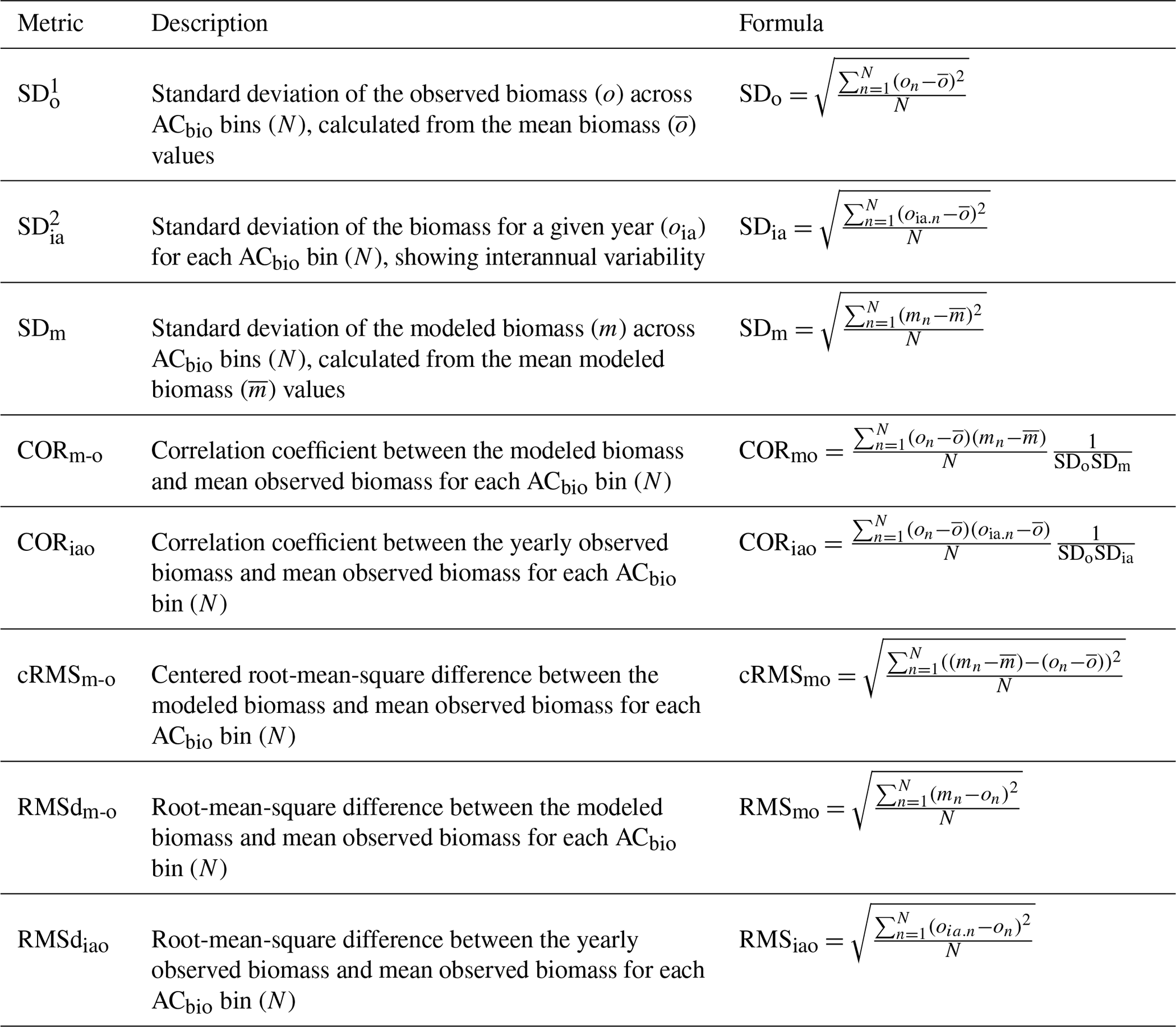
To validate the model's first-order response, we simulated conditions for CCE and station ALOHA using the reference parameters from Table 1. The results were then compared to the observed biomass spectra and nitrogen depth profiles for the two sites (Fig. 3). The contrasting oceanographic regimes between the sites are evident from their nitrogen profiles (Fig. 3a, b). The California Current Ecosystem, characterized by coastal upwelling, shows a nitricline at a depth of approximately 100 m. In contrast, station ALOHA, an oligotrophic open-ocean site with downwelling, exhibits lower nitrogen levels and a deeper nitricline. The model responds correctly to the difference in circulation at the two sites, resulting in a higher nitrogen concentration at CCE compared to station ALOHA. Although the model's results generally align with the observations, there is a depressed nitricline at CCE, leading to lower-than-expected nitrogen values in the upper 200 m of the water column and slightly elevated nitrogen concentrations at station ALOHA.

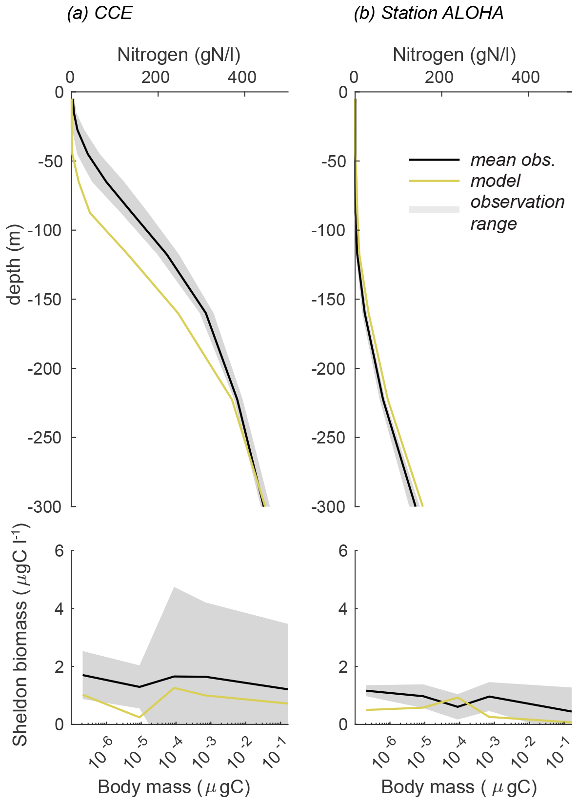
Figure 3 Nutrient profile and Sheldon biomass comparison between the observations and reference model simulation for (a) CCE and (b) station ALOHA. The Sheldon biomass spectrum illustrates the biomass in each cell mass bin normalized by the bin width. The Sheldon biomass spectrum is defined as $B_{\mathrm{s}}\left(m\right)=B_i/\log (\frac{m_i^{+}}{m_i^{-}}$) (Andersen and Visser, 2023).

Despite these differences in the nitrogen profiles, the biomass size distributions at both sites are remarkably similar (Fig. 3c, d). Both sites display a relatively flat Sheldon biomass spectrum, with mean biomasses of approximately 1 µg C L⁻¹ at CCE and approximately 0.5 µg C L⁻¹ at station ALOHA. These biomasses are within the expected range of the observations, although the mean observed biomass is slightly higher, averaging 1.5 µg C L⁻¹ at CCE and 0.5 µg C L⁻¹ at station ALOHA. Notably, the largest discrepancy between the model and observations occurs in the small size classes at station ALOHA, where the model underestimates the biomass. The larger standard deviations observed at CCE indicate a more variable environment compared to station ALOHA.

In the following, we describe the results of the first-level randomized parameter studies and the subsequent detailed studies. The shared aim of these investigations is to better understand NUM model behavior, performance relative to observations, and how much parameter choice influences model results.

4.2 First-level random parameter study: can the model reproduce the planktonic community biomass structure?

We initially tested the model's ability to reproduce the biomass spectrum and the community size spectrum of CCE. Just as importantly, this is also a test of the variable effects that parameter choices have on model results. The results of the simulations are illustrated in Taylor diagrams (Fig. 4). The Taylor diagrams provide a visual representation of the normalized standard deviation (SD_m / SD_o, radial distance from the origin shown as the solid grey line), correlation (COR_m-o, azimuthal positions), and centered root-mean-square difference (cRMS_m-o, black circles extending out from the grey dot) of the 100 000 model simulations compared to the annual averaged observations from CCE (represented by the grey dot). The bright yellow color in the first quadrants of all five diagrams shows that the model simulations generally result in a positive correlation coefficient with the CCE-LTER observations in all the biomass size categories. The smallest effect of the parameter variations is seen in the autotrophic microplankton (B_A-micro, Fig. 4e), where the solutions are centered in a smaller area than the other four size categories. On the other end of the scale, autotrophic picoplankton show the largest spread in solutions from randomizing the parameters (B_A-pico, Fig. 4c). On average, the smallest difference between the model result and the mean observations (determined as abs(1 − mean(cRMS))) is found for B_T-nano, which, despite some simulations with a negative correlation, generally shows the closest fit to the observations. The other four categories have a larger deviation from the observations due to either lower pattern agreement (COR_m-o) or overestimation or underestimation of the amplitude of variation (SD_m / SD_o). The amplitude of variation in the size spectrum is overestimated for all the size groups of picoplankton and nanoplankton, while the model underestimates the amplitude of variation in the autotrophic microplankton. The pattern agreement is overall best for B_T-pico and B_A-nano, with mean correlations of 0.87 and 0.80. Interestingly, the result of the simulations falls within three distinct groups for B_A-pico, where some parameter combinations produce a much better correlation with the observations than others. That B_A-pico falls into three groups may be related to the biomass quantization also found in the observations and other size-structured planktonic ecosystem models (Moscoso et al., 2022; Schartau et al., 2010).

Figure 4 Taylor diagrams for 100 000 random parameter combinations at CCE, displaying the standard deviation (SD) of the model result relative to the observations (Obs.) as well as the correlation coefficient (COR) and centered root-mean-square difference (cRMS) between the model and observations. The blue to yellow colors reflect the increasing number of realizations in each area. B_T and B_A are defined in Fig. 2.

An alternative way of getting an overview of the model's capabilities and parameter effect is to visualize the overall trend in simulations compared to the observation data as a density plot (Fig. 5). The coloring in the figure shows that most of the simulations for the five size categories have a power law increase in the biomass with increasing AC bins. Generally, the model does not capture the occurrences of high AC_bio concentrations (AC_bio above approximately 100 µg C L⁻¹), which is consistent with the observation that only 2 % of the samples have autotrophic biomass concentrations of 100 µg C L⁻¹ or above, illustrated here by the sizes of the white dots. The trend in the simulations corresponds relatively well to the observations for B_T-nano (compared to the mean observations given as white dots), which also proved to be the size category with the lowest cRMS (Fig. 4). The trend in B_A-nano simulations also aligns reasonably well with the observations, though the correlation is slightly weaker due to a larger discrepancy between the modeled increase in biomass and the observed increase in biomass. Both size groups of nanoplankton do however underestimate the biomass in low-AC_bio bins (AC_bio < 10 µg C L⁻¹) and overestimate the biomass at higher AC_bio, which corresponds to the higher-than-observed amplitude of variations in the Taylor diagrams. The picoplanktonic size groups also exhibit a gradual increase in biomass with increasing AC_bio rather than the plateau at intermediate to high AC_bio seen for observations of B_T-pico and the decrease in biomass for B_A-pico. Additionally, the model underestimates biomass at low AC_bio for both picoplanktonic size groups. The modeled amplitude of variation for B_A-micro is lower than the observations, which manifest as an overly high biomass at low AC_bio and a lower-than-observed increase in biomass with increasing AC_bio.

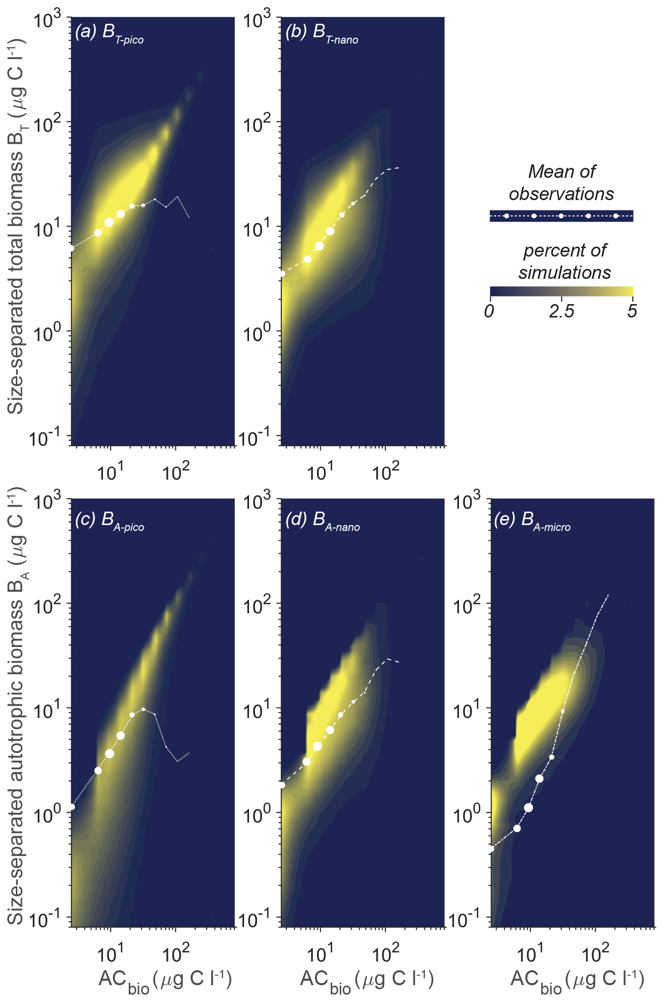
Figure 5 Model mean and total biomass of the size groups as a function of the total biomass for 100 000 random parameter combinations at CCE. The white dots are observations in AC_bio bins. The abbreviations are as in Fig. 2. Blue to yellow reflect an increasing number of realizations in each area. The sizes of the white observation dots indicate the relative number of observations in that AC_bio bin. Note the tendency of NUM to underestimate picoplanktonic (a, c) and nanoplanktonic (b, d) biomass at low AC_bio while overestimating the biomass at intermediate to high AC_bio. The autotrophic microplanktonic biomass (e) is generally overestimated.

Of the completed model calculations, the ideal parameter combinations should result in COR_m-o > COR_iao and RMSd_m-o < RMSd_iao for all the size groups. Evaluating these conditions shows that none of the model results fulfills both criteria for all the size groups. A detailed examination of the simulations in terms of COR_m-o and RMSd_m-o, however, reveals a subset of seven simulations that results in a planktonic size variability that corresponds particularly well to the observations (Fig. 6).

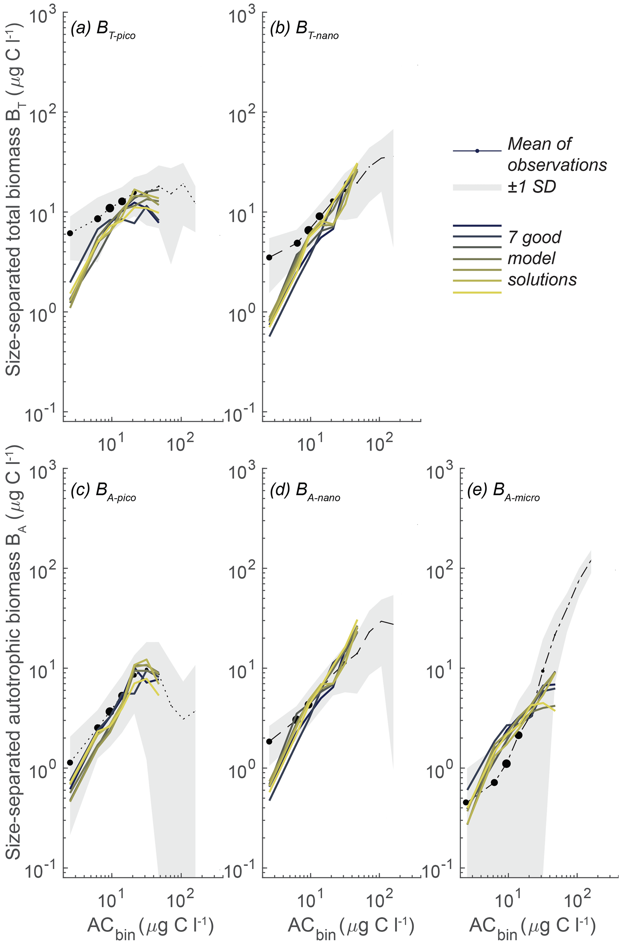
Figure 6 Model mean and total biomass of the size groups as a function of total biomass for the seven statistically most optimal parameter combinations at CCE. The black dots are observations in AC_bio bins, and the sizes of the black observation dots indicate the relative number of observations in that AC_bio bin. The abbreviations are as in Fig. 2. Note the tendency of NUM to underestimate picoautotrophic and nanoautotrophic biomass at very low AC_bio and to overestimate microautotrophic biomass.

In these seven simulations the picoplanktonic size groups align with the mean observations, showing a plateau at intermediate to high AC_bio for B_T-pico and a tendency for biomass to decrease for B_A-pico at AC_bio above 30 µg C L⁻¹ (Fig. 6a, c). The parameter combinations do however result in a B_T-pico that is lower than 1 standard deviation for the smallest AC_bio bin. Both nanoplanktonic size groups closely follow the observations, though still with lower-than-observed biomass at low AC_bio (Fig. 5b, d). The trend in microautotrophic biomass aligns with most of the model results, which generally show higher-than-observed biomass. These results are at the lower end of the 100 000 simulations but are still too high at low to intermediate autotrophic biomass levels (approximately 4–30 µg C L⁻¹), forming a “humpback” shape (Fig. 5e). While these seven simulations correlate remarkably well with the observations, they generally have a slightly too low correlation coefficient for B_A-micro (0.79–0.95 for the model results versus 0.96 for the observations) and overly high root-mean-square differences for B_T-pico (0.48–0.64 versus 0.4) and B_T-nano (0.37–0.71 versus 0.3) (the statistic is available in Sect. S3).

With the goal of identifying a parameter range that yields robust optimal solutions, in further sensitivity analyses of the parameters we will focus on this subset of seven simulations that perform especially well. We use the seven identified sets of parameters to define a restricted parameter span based on the minimum and maximum of each parameter in the set group (Fig. 7, blue lines).

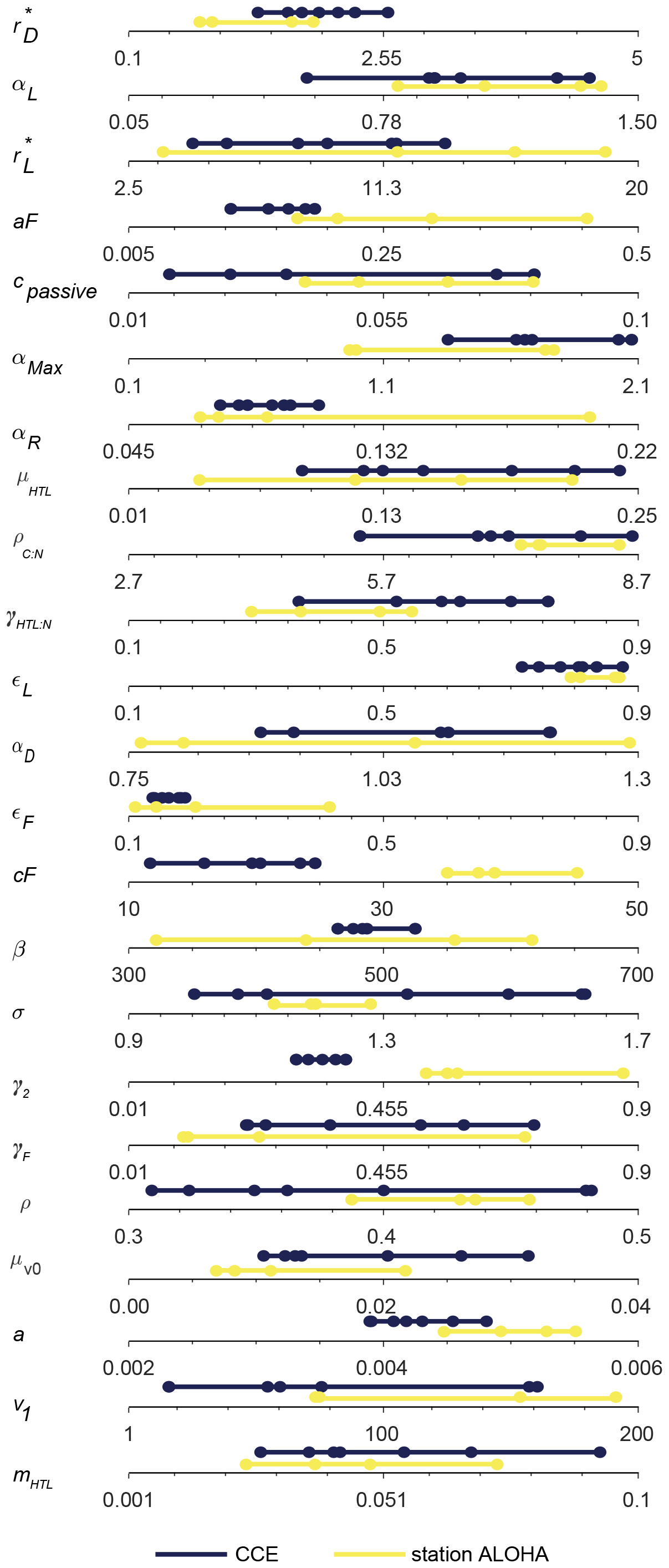
Figure 7 Span of all the free model parameters for the seven most optimal parameter combinations at either CCE (blue) or station ALOHA (yellow). The seven CCE model results are shown in Fig. 6. Note how the parameter spans for CCE and station ALOHA generally follow the same trend, except for γ₂ and cF, where higher values are needed to fit the data at station ALOHA than at CCE. The most optimal parameter combination is estimated simultaneously by the highest correlation coefficient and the lowest root-mean-square difference between the model and observations for B_T-pico, B_T-nano, B_A-pico, B_A-nano, and B_A-micro. The parameter definitions are in Table 1, and the other abbreviations are in Fig. 2.

4.3 Restricted parameter span and sensitivity

We will now aim to evaluate the importance of the parameter uncertainties and to establish a stable parameter space for the 23 free parameters where the simulations yield a reasonable result. The range of each free parameter is based on the range defined by the seven solutions with optimal fits (Fig. 6). An initial local parameter sensitivity assessment revealed a high degree of nonlinearity in the model that makes it difficult to draw any global conclusions about parameter influence based on local studies. To gain more insight into how the parameters influence the sensitivity of the entire nonlinear ecosystem, we instead perform a global sensitivity analysis (Bilal, 2014; Sobol, 2001; Zhou and Lin, 2008).

Figure 8 displays the parameters ranked by Sobol's total sensitivity index (STi) based on the root-mean-square difference for the five size groups. The corresponding figure based on correlation is available in Sect. S6, but its conclusions are consistent with Fig. 8. The value of the index cannot be compared across the different categories, but the span in values gives an indication of the variability in the sensitivity across the parameters. For example, while B_T-pico seems to be especially sensitive to approximately half of the parameters, there is little difference in parameter sensitivity for B_A-micro. The global sensitivity analysis reveals that all of the size groups are sensitive to the choice of parameters that control mortality (red dots): phagotrophy (the phagotrophic assimilation rate ε_F, clearance rate aF, predator–prey ratio β, and width σ), higher trophic level mortality (HTL pressure μ_HTL), and viral lysis (μ_v0). All of the size groups are also sensitive to the value of the maximum rate of biosynthesis (α_max) and, to a lesser degree, respiration (α_R) (grey dots). Parameters such as the remineralization rate of dead organisms (γ₂, purple), diffusive affinity crossover ($r_{\mathrm{D}}^{*}$ except for B_A-micro, blue), and C:N ratio of the cell are among the moderately sensitive parameters. The parameters mentioned above are ones that control the predation pressure, biosynthesis, and nutrient availability and uptake. Finally, the analysis shows that the picoautotrophic biomass is more sensitive to the light uptake efficiency (ε_L, yellow) parameter than the other size groups. The analysis shows that other parameters are less important and therefore allows for higher uncertainties. These parameters include the carbon density of the cell (ρ), the passive losses coefficient (c_passive), remineralization of feeding losses (γ_F), and higher trophic levels (γ_HTL).

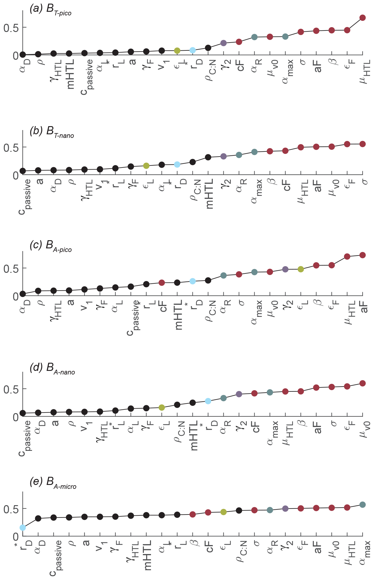
Figure 8 Global parameter sensitivity ranked based on the sensitivity index calculated by Sobol's variance-based sensitivity method for nonlinear models. Sensitivity is calculated for RMSd. The parameters that the NUM model is most sensitive to have been colored according to categories: predation and mortality (red), synthesis (grey), cell remineralization (purple), light uptake efficiency (yellow), and diffusive affinity crossover (blue). Note how all of the biomass sizes are especially sensitive to parameters controlling predation (red dots) and synthesis (grey dots). The parameter definitions are in Table 1, and the other abbreviations are in Fig. 2.

While the model sensitivity to parameters is complex and nonlinear, a final set of 10 000 random parameter simulations demonstrates that the model result space can be reduced by confining the parameter space to the restricted parameter span in Fig. 7. Using the restricted parameter span, we see a tighter fit of the model results to the observations (Fig. 9), in contrast to the full randomized parameter spans (Fig. 5). The parameter restrictions have removed the simulations that produced excess pico- and nano-sized biomass at high AC_bio, and the simulations now follow the observed trend with an onset of a plateau at AC_bio of 20 µg C L⁻¹ for B_T-pico and B_A-pico. The restriction has had less impact on the nanoplanktonic biomass but has narrowed the range of results, leading to a slight overestimation of nanoplanktonic biomass in most of the simulations, particularly at AC_bio levels above 30 µg C L⁻¹. Overall, the model results in Fig. 9 demonstrate a notable improvement in model performance for the identified parameter spans in comparison to the full parameter space. While this improvement may seem intuitive, it is not necessarily a priori given, considering the model parameters' nonlinear response to parameter change. The local sensitivity analysis showed that, even within the restricted parameter space, the impact of varying a parameter is highly dependent on the other parameters (Fig. S2). The restricted parameter space could therefore, in theory, have resulted in the same degree of model misfit as the full parameter span, with only a few acceptable solutions generated by very specific parameter combinations. That the model performance is enhanced by restricting the parameter span suggests that further detailed parameter tuning may not be necessary to achieve reliable results from the NUM model. While a better performance is encouraging, it is important to evaluate whether the identified parameter spans are applicable to other biogeographic provinces.

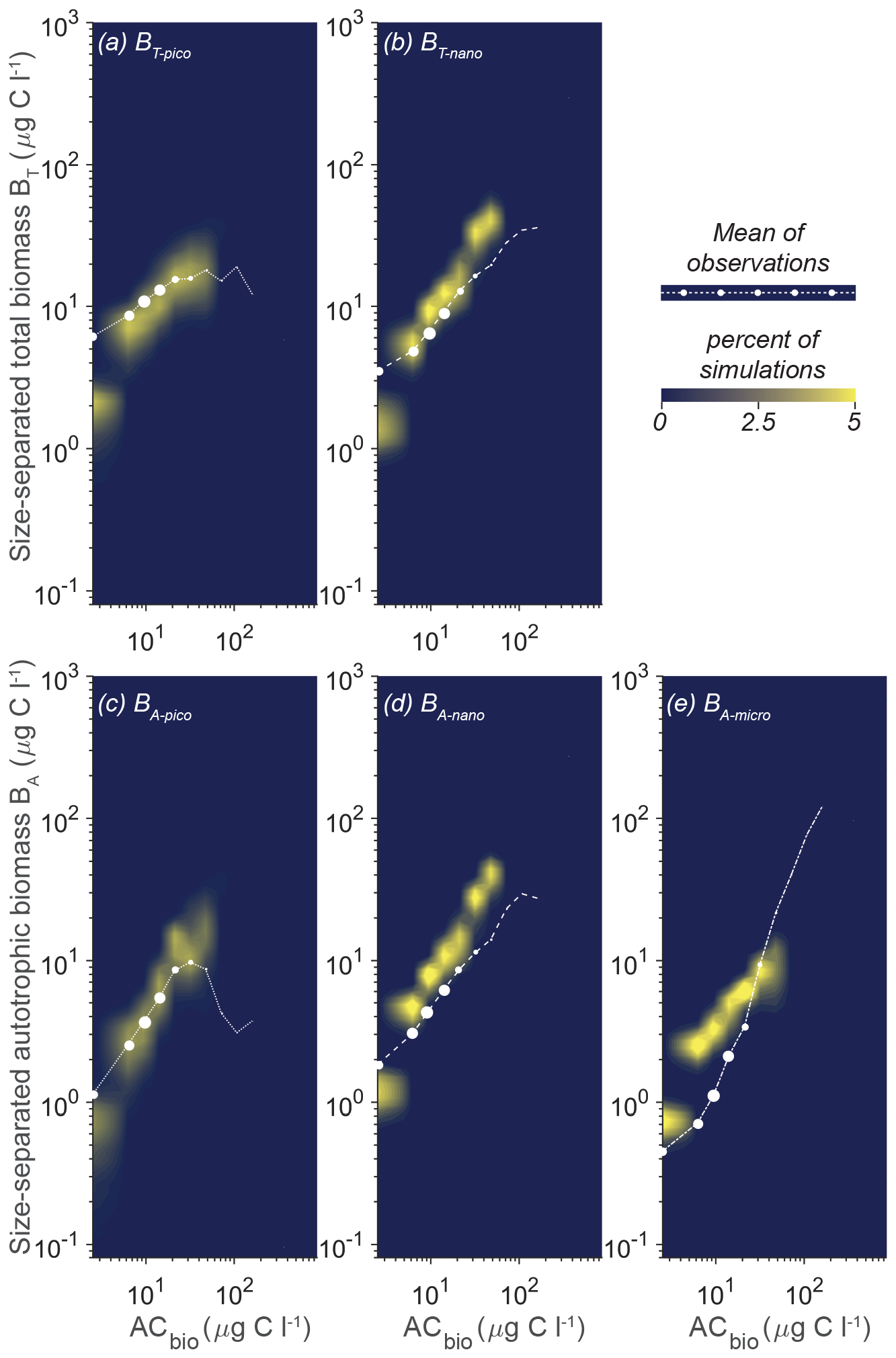
Figure 9 Model mean and total biomass of the size groups as a function of the total biomass for 10 000 random parameter combinations sampled within the restricted span of parameters at CCE. The random parameter spans are based on the parameter range of the seven statistically optimal parameter combinations at CCE (see the text). The white dots are observations in AC_bio bins, and the sizes of the white observation dots indicate the relative number of observations in that AC_bio bin. The abbreviations are as in Fig. 2. Blue to yellow reflects an increasing number of realizations in each area. Note how the solution space has been restricted, especially for picoplankton (a, c), compared to the full parameter span (Fig. 5).

4.4 Results for station ALOHA

The heart of the trait-based approach is its potential universality, the principle that a single set of parameters can describe organisms and ecosystems across time and place. An important test is therefore whether the parameter sets that performed best at CCE are suited to different oceanographic settings. Figure 10 shows the result of 10 000 simulations, with the conditions mimicking station ALOHA with quasi-random parameters from within the restricted parameter span defined for CCE. The model reacts to the shift in oceanographic regime by lowering the overall autotrophic biomass. Most simulations only reach a biomass of 20 µg C L⁻¹, which is consistent with observations. The biomass of the picoplanktonic size groups is lower than the mean observation but is generally within 1 standard deviation (Fig. 10a, c; see Fig. 2b for comparison). Both nanoplanktonic size groups exhibit elevated biomass relative to the observations, with the discrepancy being larger than that observed for the nanoplanktonic size groups in the CCE simulations (Fig. 10b, c; see Fig. 9b, c for comparison). The microautotrophic size group exhibits the poorest correlation with the mean observations, displaying excessive biomass at low AC_bin (< 9 µg C L⁻¹) and variable but lower biomass at AC_bin above 9 µg C L⁻¹. This pattern is inconsistent with the observed sigmoidal trend, although the biomass falls within the standard deviation of the observations (Fig. 10e; see Fig. 2b for comparison). A comparison to the first-level random parameter simulation with 100 000 simulations within the full parameter space (not illustrated here but available in Sect. S7) shows that restricting the parameters based on the solutions from CCE has removed a set of simulations that produced overly large biomasses for all the size categories at intermediate AC bins. However, it also eliminates a set of simulations with better-fitting biomass concentrations at low-AC_bio bins. Figure 11 shows a set of simulations from the first-level random parameter study that performs particularly well for station ALOHA. In these simulations, both picoplankton and nanoplankton follow the trend of the observations and exhibit the correct amount of biomass. Interestingly, most of the parameters for these four simulations fully overlap with the parameters for the best solutions at CCE (Fig. 7). While some parameters such as aF and α_max only partly overlap, the only parameters that differ significantly between the two sites are γ₂ and cF, which both have higher values at station ALOHA than at CCE. The parameter γ₂ controls the fraction of dead matter directly remineralized back to nutrients, and it is therefore an important parameter for controlling the amount of osmotrophy for the smallest planktonic size group. cF and aF are two important components of the rate of phagotrophy. It is noteworthy that the parameters for successful solutions at the two different sites exhibit trends that in many cases are correlated; for both stations, the successful simulations have relatively high α_L,α_max, ρ_C : N, ε_L, and a values and a low ε_F value.

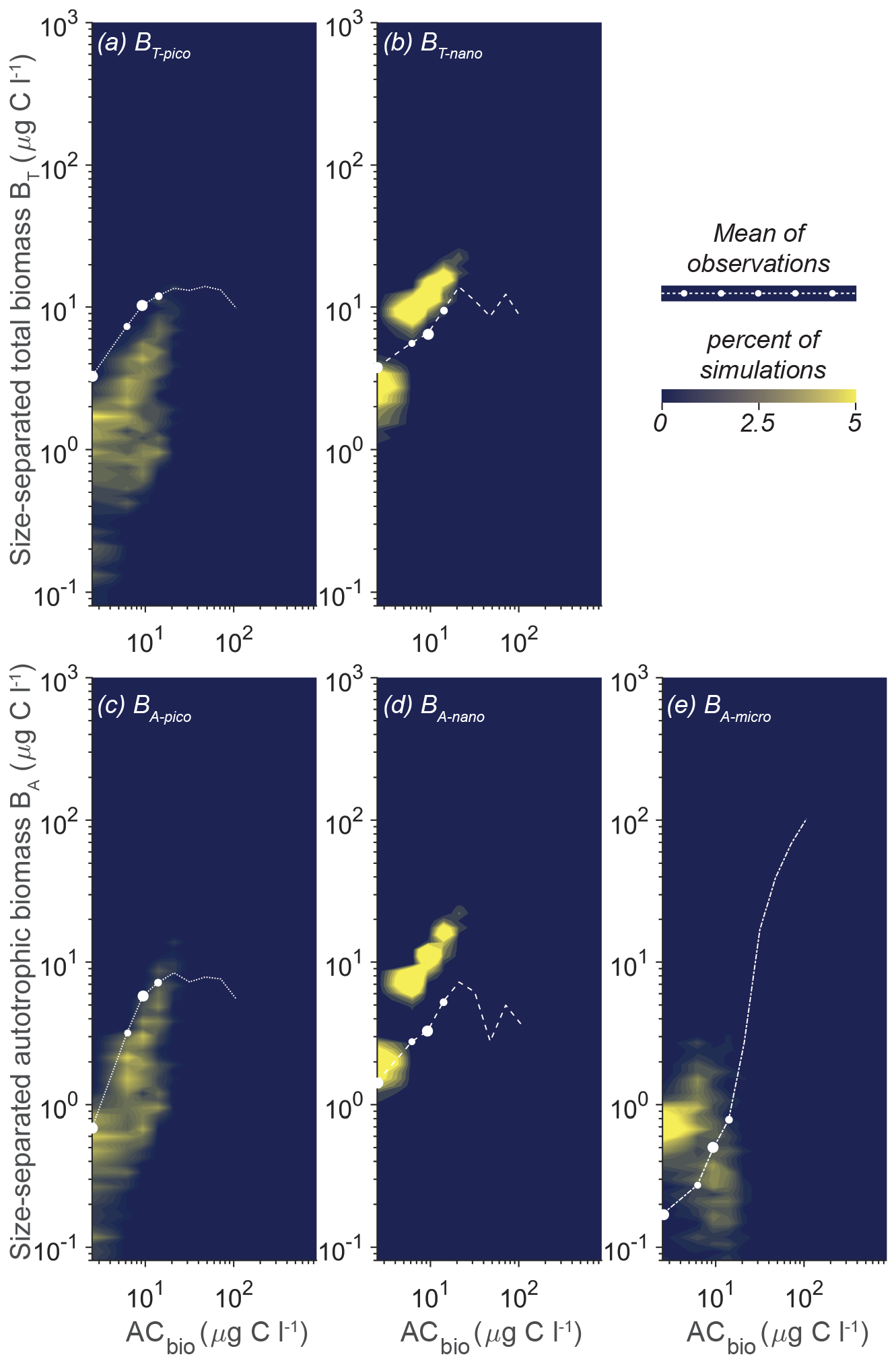
Figure 10 Model mean and total biomass of the size groups as a function of the total biomass for 10 000 random parameter combinations at station ALOHA. The simulations have random parameter combinations within the restricted parameter space based on the successful simulations from CCE (Fig. 7). The white dots are observations in the AC_bio bins, and the sizes of the white observation dots indicate the relative number of observations in each AC_bio bin. The abbreviations are as in Fig. 2. The blue to yellow colors reflect an increasing number of realizations in a given area. Note how the biomass of picoplankton (a, c) is underestimated, while nanoplankton (b, d) is generally overestimated. Microautotrophic plankton (e) have the lowest correlation of the five size classes, with decreasing biomass as a function of AC_bio.

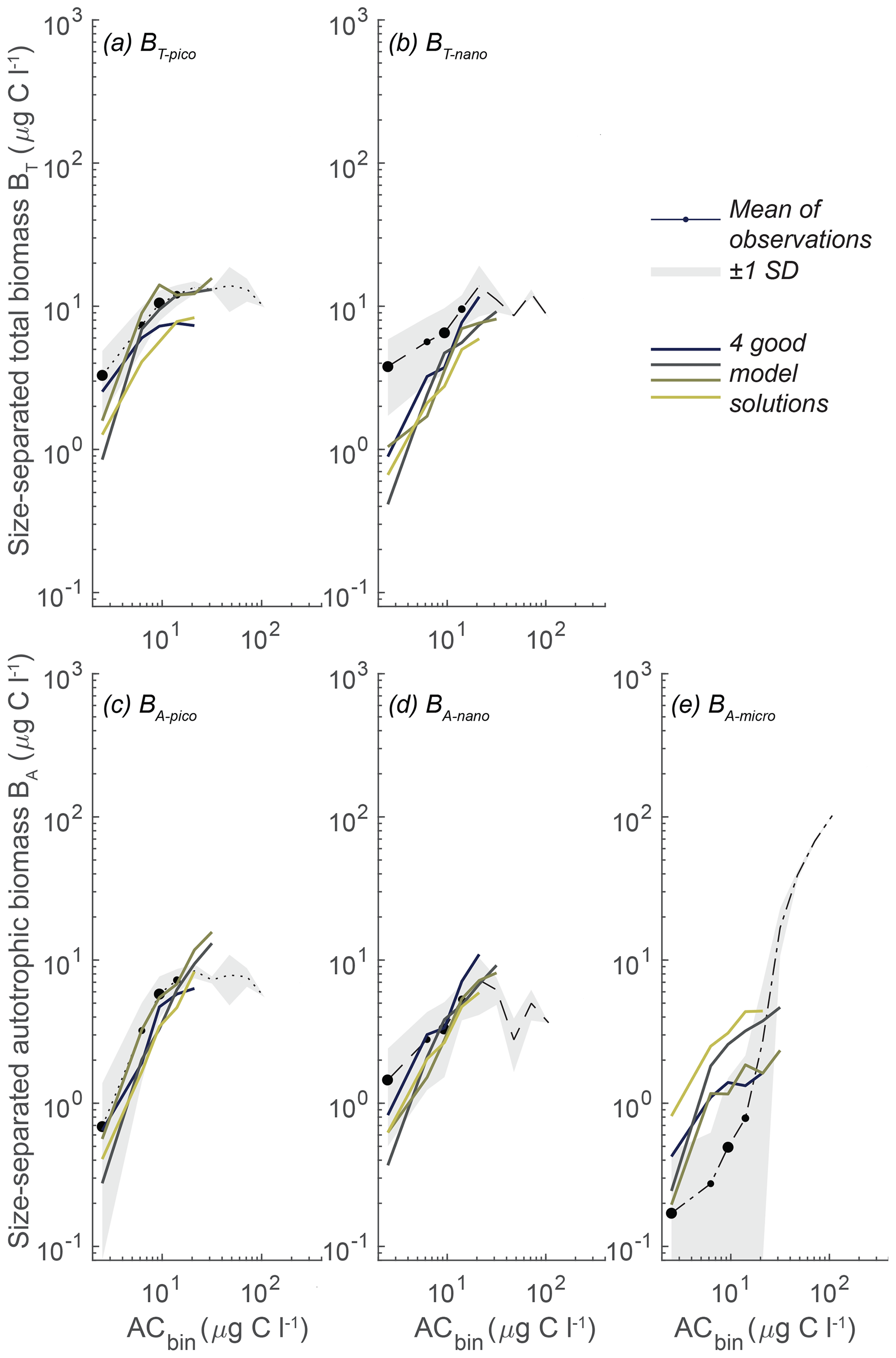
Figure 11 Model mean and total biomass of the size groups as a function of the total biomass for the four statistically most optimal parameter combinations at station ALOHA. The black dots are observations in AC_bio bins, and the sizes of the black observation dots indicate the relative number of observations in that AC_bio bin. The abbreviations are as in Fig. 2.

4.5 Nutrient profiles

As an indirect way of evaluating the model performance and response to the different environmental conditions, we also evaluate the depth profile of model nutrients for the two sites (Fig. 12). Importantly, the nutrient profile was not part of the initial statistical measures used to identify the model parameters. The nutrient profiles for CCE are remarkably consistent across the solutions. Nutrient concentrations are low in the upper photic zone and increase with depth. While the modeled profiles generally align with the observed data, there is a tendency to underestimate nitrate concentrations at depths ranging from 50 to 200 m. For station ALOHA, the modeled profiles also align well with the measured concentrations, with a slight tendency to overestimate nutrient concentrations at depth. The model is generally able to respond correctly to the shift from eutrophic to oligotrophic conditions.

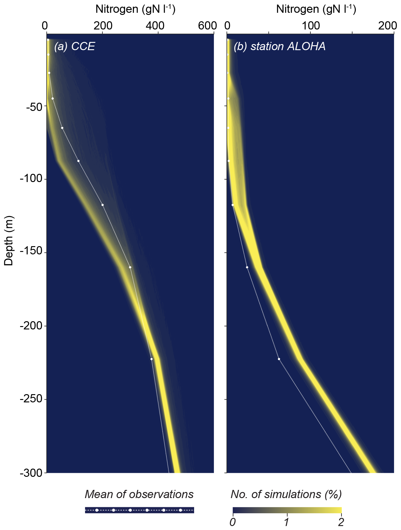
Figure 12 Model nutrient profiles at CCE (a) and station ALOHA (b). The white dots are observations based on CalCOFI-Scripps-Institution-of-Oceanography and Wilkinson (2022), Pasulka et al. (2013), and Garcia et al. (2018). Note the model tendency to underestimate N in the thermocline at CCE but overestimate it at station ALOHA.

5 Discussion and perspectives

5.1 Summary of the model performance

We have validated the generalist unicellular NUM ecosystem model for two quite different biogeographic provinces: the high-productivity upwelling conditions of the California Current Ecosystem and the oligotrophic downwelling conditions at station ALOHA. For the California Current Ecosystem, out of 100 000 random combinations of the 23 free parameters, a large majority of the model results have correlation coefficients for observations (COR_m-o) greater than 0.7. This demonstrates that the generalist unicellular NUM model, despite its simplicity, can capture the size distribution of the planktonic ecosystem and its nutrient profile over a broad range of parameter values. Out of the random simulations we find only seven optimal, but quite different, parameter combinations that reproduce results for CCE. These seven optimal simulations almost perfectly match the distribution of each of the size groups as a function of increasing AC_bio (Fig. 6). The seven optimal parameter combinations have a mean COR_m-o of 0.94 and an RMSd_m-o of 0.4 for the five size groups considered in comparison with the observations. In particular, we find a B_A-pico peak and a B_T-pico plateau at intermediate levels of autotrophic biomass, in agreement with the observations (Taylor and Landry, 2018) (Fig. 6a, c). We also find a power law increase in B_T-nano and B_A-nano as a function of AC_bio, as in the observations (Fig. 6b, d). Finally, we observe a humpback increase in B_A-micro that has the lowest correlation with the observations but that is still within 1 standard deviation of the observed total mean (Fig. 6e).

Moving to the oligotrophic station ALOHA, we find that the seven optimal model parameter combinations from CCE give model results that capture many important aspects of the observational data. NUM qualitatively models a reduction in biomass at station ALOHA relative to CCE and generally reproduces the overall size structure. That the NUM model produces less biomass at ALOHA is consistent with observational differences between CCE and ALOHA (Taylor and Landry, 2018). The seven simulations do however produce overly low picoplankton biomasses and overly high nanoplankton biomasses compared to the observations. A detailed analysis shows that another set of parameter combinations was better at reproducing the picoplankton and nanoplankton biomasses in terms of both correlation and overall biomass values. The parameter spaces for these simulations were only significantly different from the restricted parameter span for CCE in their range of a few parameters (discussed below). Our validation against ALOHA indicates overall that, by restricting the parameters based on the seven optimal models at CCE and focusing on this small set of parameters, it is possible to match the overall increase and decrease in biomass for the different size classes to a degree that would be satisfactory for applications where site-by-site calibration is not possible.

5.2 Parameter sensitivity

Our sensitivity analysis shows that the model parameter sensitivity is dependent on the specific parameter combinations and that the ecosystem response is nonlinear. Local sensitivity analysis revealed that, while one of the good solutions was nearly equally sensitive to almost all of the parameters, another was mainly sensitive to only one parameter (εF, Fig. S2 in Sect. S4). Through a global sensitivity analysis, we identified the parameters that are especially controlling (Fig. 8). Parameters regulating predation, mortality, biosynthesis, and respiration are generally important among all the size groups. Changes in these parameters create the largest shifts in the model output. Interestingly, many of the parameters that produce the largest shifts in biomass are also among the least constrained (Table 1; Andersen and Visser, 2023). In the following discussion, we focus on the parameters that are the least constrained but that also result in the highest sensitivity. Higher trophic level mortality (μ_htl) is important for all the size groups. μ_htl is an extrinsic parameter that governs predation rates at higher trophic levels. This parameter serves as a closure term in the model and plays a critical role in shaping the biomass distribution. Specifically, μ_htl determines the size and biomass of microplankton, initiating cascading effects on smaller size classes. While μ_htl significantly impacts biomass partitioning across the size groups, its influence on the total biomass is limited because reductions in microplankton result in corresponding increases in nanoplankton (see Fig. 15b in Andersen and Visser, 2023). The value of μ_htl depends on the biomass and efficiency of the higher trophic levels, which can vary significantly between eutrophic and oligotrophic environments. Our results indicate that the optimal μ_htl is larger at CCE than at station ALOHA, although there is a significant overlap (Fig. 7). The importance of μ_htl suggests that including higher trophic levels, such as copepods, could reduce model uncertainties. However, that only shifts the problem towards determining the higher trophic level mortality pressure on copepods, which is equally uncertain. Another highly uncertain parameter that creates a large shift in the biomass distribution is the viral lysis mortality coefficient μ_v0. This parameter introduces a density-dependent control of the population in each size group. It has the effect of increasing the mortality pressure on groups with high biomass and prevents all biomass from ending up in one or a few size groups. The principle of abundance-controlled viral lysis is an important aspect of the “killing the winner” principle (Thingstad, 2000; Winter et al., 2010). The default parameter used in the NUM model is adjusted such that the effect of viral lysis is smaller than that of other mortalities, in order to prevent this process from determining the result despite the value of the parameter being largely unknown. Based on the global sensitivity study, it will be an important future priority to get a better mechanistic understanding of the viral lysis mortality process. Two other important parameters, cF and εF, are involved in heterotrophic phagotrophy and are partly multiplicative, so one influences the other (Eq. 3, Table 2). While the assimilation efficiency (εF) is relatively well-constrained, the maximum phagotrophic coefficient (cF) is not. The parameter cF is unique to the NUM model and determines the phagotrophic assimilation limit for large cells. While cF only directly influences the largest cells, it causes a cascading effect down the size spectrum. The default value used here is fitted against the maximum growth rates for different types of plankton (see Fig. 5 in Andersen and Visser, 2023). Interestingly, cF is one of the only parameters that show significantly different optimal values for CCE and station ALOHA (11–25 µg d⁻¹ for CCE and 35–45 µg d⁻¹ for station ALOHA). The difference is likely related to a tradeoff between food acquisition and predation, which is an important aspect of the slow–fast tradeoff (Salguero-Gómez et al., 2016; Kiørboe and Thomas, 2020). High rates of predation induce higher food acquisition but come with a higher predation risk (Kiørboe and Thomas, 2020). The difference between CCE and station ALOHA can therefore be seen as a difference between a more stable environment with high population densities (CCE) and varied conditions with strong environmental gradients (station ALOHA). The same argument is valid for the phagotrophic clearance rate (aF), where the good fit for station ALOHA has higher values compared to CCE. The mechanistic argument for phagotrophic clearance rates relates to the fluid dynamics of a beating flagellate cell (Nielsen and Kiørboe, 2021; Andersen and Visser, 2023). This mechanistic underpinning means that the value of aF is relatively well-known, with however a scatter of 1 order of magnitude due to differences in flagella arrangements that generate differences in the predation risk. Future investigations into patterns of flagella arrangements in different nutrient environments can maybe give some valuable insight into the tradeoff between foraging and predation risk.

The last highly unknown parameter that can create large shifts in the biomass is γ₂, which determines how large a fraction of the background mortality is remineralized directly into N and DOC instead of becoming POM. Increasing γ₂ increases the amount of dissolved nutrients and carbon in the system, which increases the osmotrophic efficiency for picoplankton. However, this value of γ₂ is highly uncertain, and cell mortality is treated quite simply here because of limited mechanistic understanding (Andersen and Visser, 2023). Apart from cF, γ₂ is the only other parameter where values are significantly different between the two sites. Values for γ₂ are larger at station ALOHA than at CCE, indicating that faster remineralization of organic matter is required at station ALOHA. It is clear from the global sensitivity study that developing a clear mechanistic understanding of the fate of cell mortality should be an important priority. Fortunately, a mechanistic model for organic matter accumulation has been developed recently and may be a way to improve the NUM model accuracy in future versions (Zakem et al., 2021).

Apart from the parameters described above, the model includes better-established parameters that result in a relatively high sensitivity while also influencing the entire size spectrum. Of these, σ, β defines the shape of the prey–predator size distribution, and α_max, α_R controls the biosynthesis. In contrast, the effect of ε_L (light uptake efficiency) mainly influences picoplankton's affinity for photosynthesis.

Despite the model's sensitivity to parameter changes, nonlinearity, and system bifurcation, it appears to be relatively stable within the optimized restricted parameter spans identified based on comparison with CCE observations. Within the restricted spans, no parameter combinations seem to perform significantly better than others for the chosen metrics. We recognize however that further local parameter sensitivity investigation can be useful with our current knowledge about the most important parameters gained from the global sensitivity study.

An underlying premise in our validation is that we compared the model results of a water column setup with annual mean observations averaging nearly 700 km by 400 km, including the shelf and open ocean. This means that any parameter combination that performs well compared to the mean dataset will surely be less than optimal at some of the individual stations or at specific times of the year. Ongoing work is evaluating the NUM model in a regional ocean model where smaller variations along the shelf and especially across the shelf can be resolved, as well as in settings where the data permit resolution of seasonal variability.

5.3 Areas for improvement

We note that the optimal parameter spans have been determined with a water column model without vertical advection. CCE is particularly influenced by upwelling advection, while station ALOHA is influenced by convergence and downwelling advection. This difference is likely a significant factor contributing to the model deficiencies at ALOHA. Indeed, the 100 000 random simulations at CCE tend to produce overly low nitrate concentrations at depths of 50 to 200 m. This indicates that the model is missing additional upwelling that could push the nutricline up. It may be reasoned that, if there had been more physical upwelling in the model, the higher nutrient loading and presumably growth would mean that a new set of optimal parameter combinations would need to result in less biomass production to fit the observed biomass. The implication of more efficient biomass downregulation by perhaps more export would mean that, for ALOHA, there would be more export, making the system more oligotrophic, further enhancing the picoplanktonic biomass, and lessening the nanoplankton and microplankton. In fact, we see in the nutrient profiles that ALOHA has overly high nutrient levels from 100 m and deeper. More downwelling advection in the model setup for ALOHA would push the nutricline down and result in a more oligotrophic system, perhaps shifting the ecosystem towards more picoplankton. Regardless, future investigations including a full two-way cross-validation should explore NUM in a 3D circulation mode to alleviate the model physics deficiencies of the current water column setup.

In the NUM model, there is only one generalist functional group where small and large are defined by the same parameter combination. This means that the smallest sizes, which are essentially bacterial, are modeled with the same set of parameters as larger eukaryotic phototrophs. It is well-known that there is a myriad of different species of bacteria optimized with different metabolic strategies, optimized with different cell membranes, and without mitochondria. For example, while the prokaryotes Synechococcus and Prochlorococcus have similar sizes, the former inhabit the surface waters at station ALOHA and the latter live under low-light conditions near the nutricline (Wu et al., 2022). Furthermore, while having quite different modes of life, their resource uptake and growth are significantly different from, e.g., those of picoeukaryotes or nanoeukaryotes. In fact, large metadata analyses show very different allometric scalings of the metabolic rate as a function of body mass (size) (DeLong et al., 2010). Prokaryotes show super-linear scaling with a power of 1.7, while eukaryote protists have linear scaling with a power of 1. Thus, empirical observations seem to suggest that the parameters regulating biosynthesis in NUM may need to respond more strongly to size at the picoplankton end of the spectrum (DeLong et al., 2010). In fact, our global sensitivity study revealed that the parameter regulating biosynthesis (α_max) is one of the most important parameters (Fig. 8). We furthermore found that the model in general could not capture picoplankton biomass in the oligotrophic system. However, the best fit between the model and observations is with low $r_{\mathrm{D}}^{*}$, which increases the efficiency of the picoplanktonic community. If biosynthesis in the picoplankton range is modeled as more efficient than for larger sizes, it potentially would up-regulate the microbial loop and result in more picoplankton biomass.

Another aspect related to too little pico-biomass under oligotrophic conditions may be the model treatment of DON (dissolved organic nitrogen). Currently the model uses DOC that only contributes to osmotrophic heterotrophy. However, labile DOM has a DOC : DON ratio of ∼ 5–15 (Zakem and Levine, 2019). This means that under oligotrophic conditions the model osmotrophic bacteria are potentially nutrient-limited, missing an important source of nutrients that could boost the pico-microbial loop and thereby increase B_T-pico. Adding an explicit or implicit treatment of labile DON would likely result in better performance (Zakem and Levine, 2019). Other recent studies have shown that the picoplankton Prochlorococcus, while predominantly phototrophic, is capable of osmotrophic mixotrophy under low-light conditions, and labile DOM additions under low light boost the growth significantly (Wu et al., 2022). The experiments reveal that significant Prochlorococcus growth and biomass in the deep chlorophyll maximum are likely sustained by both light and DOM. Such an additive substrate would increase the model picoplankton growth rate and boost B_A-pico to better match the observations.

The simplicity of the NUM model places some limitations on its use in some environments. The model does not yet include oxygen or reduction-oxidation reactions as in some trait-based models (Zakem et al., 2020b; Zakem et al., 2020a). This has implications for the large phagotrophs or higher trophic levels that are not restricted in their respiration if for example oxygen is low. Using the model below the photic zone in upwelling systems and to investigate low-oxygen environments would require implementation of oxygen, a development that is under way. The model ecosystem is not currently limited by nutrients other than nitrate, e.g., iron or phosphate (Serra-Pompei et al., 2022; Serra-Pompei et al., 2020). It might also be possible to capture more details of the ecosystem by parameterizing or adding additional functional groups such as diatoms and bacteria, but these refinements come with a computational cost. Overall, the NUM model is fast and has the benefits of being able to resolve mixotrophy in organisms and shared predation, aspects attracting increasing attention in trait modeling (Wu et al., 2022; Casey et al., 2022; Follett et al., 2022). Our analysis shows that the model – overall and despite its simplicity – is remarkably stable within a wide range of parameters and is usable for someone without intimate knowledge of the parameter settings.

6 Conclusion

We have validated the generalist unicellular component of the NUM ecosystem model framework in a water column setup for two sites – a high-productivity upwelling system and an oligotrophic downwelling system. With optimization of the range of 23 free parameters, the unicellular component of NUM, despite its simplicity, can capture the size distribution of the planktonic ecosystem and its nutrient profile over a broad range of parameter values. The model reproduces the nutrient profile reasonably despite its simple POM and degradation formulation. For CCE we find seven optimal parameter combinations that are quite different but almost perfectly match the distribution of each of the size groups as a function of increasing AC_bio. Validation against ALOHA indicates overall that, by restricting the parameters based on the optimal parameters for CCE, increasing the microbial loop (increasing γ₂), and focusing on predation, there is a reasonable match to the overall trends in biomass for the different size classes and the nutrient profile. We find that there is a tendency for NUM to underestimate picoplankton and nanoplankton biomass at both sites, indicating that osmotrophy, nutrient uptake, and/or mixotrophy in the lower range of the picoplankton group require further development.

Despite its simplicity, the NUM framework is remarkably stable within the identified restricted parameter ranges and likely well-suited to modeling poorly known regions and evolutionary scenarios where first principles trump details.