the Creative Commons Attribution 4.0 License.
the Creative Commons Attribution 4.0 License.
Virtual Integration of Satellite and In-situ Observation Networks (VISION) v1.0: In-Situ Observations Simulator (ISO_simulator)
Sadie L. Bartholomew
David Hassell
Alex M. Mason
Erica Neininger
A. James Perman
David A. J. Sproson
Duncan Watson-Parris
Nathan Luke Abraham
This work presents the first step in the development of the VISION toolkit, a set of Python tools that allows easy, efficient, and more meaningful comparison between global atmospheric models and observational data. Whilst observational data and modelling capabilities are expanding in parallel, there are still barriers preventing these two data sources from being used in synergy. This arises from differences in spatial and temporal sampling between models and observational platforms: observational data from a research aircraft, for example, are sampled on specified flight trajectories at very high temporal resolution. Proper comparison with model data requires generating, storing, and handling a large number of highly temporally resolved model files, resulting in a process which is data-, labour-, and time-intensive. In this paper we focus on comparison between model data and in situ observations (from aircraft, ships, buoys, sondes, etc.). A standalone code, In-Situ Observations Simulator, or ISO_simulator for short, is described here: this software reads modelled variables and observational data files and outputs model data interpolated in space and time to match observations. These model data are then written to NetCDF files that can be efficiently archived due to their small sizes and directly compared to observations. This method achieves a large reduction in the size of model data being produced for comparison with flight and other in situ data. By interpolating global gridded hourly files onto observation locations, we reduce data output for a typical climate resolution run, from ∼3 Gb per model variable per month to ∼15 Mb per model variable per month (a 200-times reduction in data volume). The VISION toolkit is relatively fast to run and can be automated to process large volumes of data at once, allowing efficient data analysis over a large number of years. Although this code was initially tested within the Unified Model (UM) framework, which is shared by the UK Earth System Model (UKESM), it was written as a flexible tool and it can be extended to work with other models.
- Article
(2317 KB) - Full-text XML
- BibTeX
- EndNote
The importance of atmospheric observations from both in situ and remote sensing platforms has been growing in the last few decades, with data archives, such as the new Natural Environment Research Council (NERC) Environmental Data Service (EDS; https://eds.ukri.org, last access: 8 January 2025), becoming a key infrastructure for the storage, exchange, and exploitation of data. The strategic importance of in situ measurements was also highlighted by the recent GBP 49 million NERC funding to maintain and re-equip the BAe-146 research aircraft of the FAAM Airborne Laboratory out to 2040 (https://www.faam.ac.uk/mid-life-upgrade/, last access: 8 January 2025).
Advances in geophysical model developments and exascale computing have similarly led to an increase in the complexity of models used for climate projections in international modelling projects, such as CMIP6; chemistry and aerosol components are now routinely being included in a number of climate model simulations (Stevenson et al., 2020; Thornhill et al., 2021; Griffiths et al., 2021). Comparing all these models with observations is vital to increase our confidence in their ability to reproduce historical observations, to understand existing biases, and ultimately to improve their representation of the atmosphere.
A wide variety of observational datasets can be used for model evaluation; what makes such comparisons with model data inherently difficult is the difference between the orderly model data, defined on the model grid at regular time intervals, and the unstructured observational data, with variable coverage in space and time. A large computational effort is required for the handling and processing of gridded model data files into a format suitable for direct comparison with observations, especially when the measurement location varies with time (e.g. aircraft, ships, sondes). In order to compare this to observational data with varying coordinates, model output must include hourly (or higher-frequency) variables over a large atmospheric domain. As well as being data-intensive, extracting hourly data from a tape archive is also time-intensive. This leads to orders of magnitude more data being stored and processed than is actually required, and a significant number of labour and computer resources are spent to extract, read, and interpolate model data in space and time onto desired observation coordinates. Because of these issues, previous studies of comparison between models and in situ observations from aircraft are generally restricted to case studies over a limited number of campaigns (e.g. Kim et al., 2015; Anderson et al., 2021), or they compare model data with observed data independently of the time or location of measurement (e.g. Wang et al., 2020).
A previous attempt at producing Unified Model data on flight tracks was made several years ago, by embedding a flight_track routine (using Fortran programming language) within the UM-UKCA source code (Telford et al., 2013). However, using this approach added a computational burden to the running of the UM-UKCA model, and it was mainly intended for the output of chemical fields (model diagnostics related to some UM dynamical fields were not available within the UM-UKCA subroutines). As a result, the flight_track routine used in Telford et al. (2013) was never ported to further versions of UM-UKCA.
In this paper we describe the first tool in the VISION toolkit: ISO_simulator.py. This code can be embedded into the model workflow, or it can optionally be used as a standalone code with existing model data (e.g. to process variables from existing simulations). When ISO_simulator is embedded in the model workflow, it produces much smaller data files which can easily be archived and are ready to be used for direct comparison with observations.
This new tool allows the routine production of model data interpolated at the time and location of in situ observational data. This can enable the exploitation of large observational datasets, potentially spanning decades, to be used for large-scale model evaluation. Another possible application of the VISION toolkit is for improving model comparison with observations when conducting Observing System Simulation Experiments (OSSEs) (Zeng et al., 2020). These experiments are typically performed using models with a high spatial and time resolution; integrating the VISION tools into the workflow of such high-resolution nature runs (NRs) would allow us to efficiently sample data at the model time step with much-reduced data storage requirements. Whilst the UM/UKESM has been used as a test model and the current version of the tool is designed to work with UM output, the next version of the VISION toolkit (currently under development) will be model-independent. Since VISION is designed to work with CF-compliant data, including CMIP CMORised output, it could provide a valuable tool for supporting expanded diagnostics in upcoming CMIP7 experiments.
In Sect. 2 we describe the ISO_simulator code, including command line arguments, input–output files, and code optimisation. In Sect. 3 we show how ISO_simulator is embedded within the Unified Model workflow. In Sect. 4 we provide some example plots showing comparisons of UM–UKESM-modelled ozone to measurements from the Cape Verde Atmospheric Observatory (CVAO) (Carpenter et al., 2024), ozone measurements from the Tropospheric Ozone Assessment Report (TOAR) ocean surface database (including data from cruise ships and buoys, similar to Lelieveld et al., 2004, and Kanaya et al., 2019), and ozone measurements from the FAAM Airborne Laboratory (Smith et al., 2024) and the NASA DC-8 Atmospheric Tomography (ATom) mission (Thompson et al., 2022).
In order to run ISO_simulator.py v1.0, the user will need access to Python 3.8 or higher, including CIS v1.7.4 (Watson-Parris et al., 2016), cf-python v3.13.0 (Hassell and Bartholomew, 2020), and Iris v3.1.0 (Hattersley et al., 2023) APIs. Iris libraries are used in some CIS functions to read gridded model data.
ISO_simulator.py performs the following steps:
-
Reading time and coordinates from observational files using CIS Python libraries,
-
Reading all model variables from hourly files using cf-python libraries,
-
Co-locating model variables in space and time to the same time/location as the observations using CIS Python libraries,
-
Writing monthly NetCDF files (Rew et al., 1989) containing model variables co-located onto flight tracks.
2.1 Input arguments
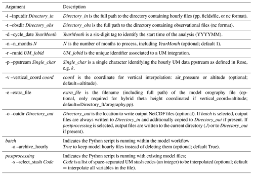
ISO_simulator.py requires a number of command line arguments which are shown in Table 1. The current version of ISO_simulator was developed for use within the UM modelling framework; therefore some of the current command line arguments are UM-specific. However, when interfacing ISO_simulator to different models, these command line arguments can be changed to reflect output data that are specific to each model.
A subparser argument, “jobtype”, is used to indicate whether the code is running within a model runtime workflow (if “batch” is selected) or as a standalone postprocessing tool, e.g. on existing model data (if “postprocessing” is selected). These subparser arguments also unlock specific conditional arguments: –archive_hourly can be used only if “batch” is selected, and –select_stash can only be used if “postprocessing” is selected. By default, when running in batch mode, all fields present in the output file being processed will be co-located to the observational locations.
2.2 Required input files
Model input files can be supplied in NetCDF, UM pp, and UM fieldsfile formats and must have a date tag in the filename (YYYYMMDD) to identify the date in the file. The ability to read different formats of model input files gives extra flexibility to the code, as it allows one to read both other model data and UM data.
The interpolation code can use either air_pressure or altitude as the vertical coordinate for interpolation. If this is not specified, it will use altitude by default. When using air_pressure as a vertical coordinate, model variables are output on selected pressure levels. Since the UM has a terrain-following, hybrid-height vertical coordinate system, we additionally need to output a Heaviside function that accounts for missing model data where a pressure level near the surface falls below the surface height for that grid box. Where data are valid, the Heaviside function has a value of 1, and it has a value of 0 otherwise. By dividing the model field on pressure levels by this Heaviside function, the model data are correctly masked and missing data are assigned to invalid grid points.
When using altitude as a vertical coordinate, because of the UM hybrid height coordinates, model variables are defined at specified heights above the model surface; therefore, the model orography field has to be provided to correctly convert the model hybrid height to altitude above sea level. The name and path of the orography file can be defined using the -e command line argument.
For observational data which are defined at the surface (ground measurements or ship/buoy data), a vertical coordinate is generally not provided. In this case, ISO_simulator will use the model lowest level and interpolate in time, latitude, and longitude only.
Along with model files, input files containing information on the observational data coordinates are also required. These input files should be in NetCDF format (Rew et al., 1989), all data should be organised into daily files, and each file must have a date tag in the filename (YYYYMMDD) to identify the date of the measurement. Along with time and positional coordinates, an optional string variable can be added to the observational input files to identify data belonging to a specific dataset or campaign; this can help during analysis to subset-relevant data, which is useful when comparing to several datasets/campaigns over a number of decades. Existing observational data might require a degree of pre-processing to ensure files are in the right format to be used by ISO_simulator; the extent and type of processing will vary depending on the format and structure of each observational dataset.
2.3 Output files
The model data, co-located to the observational coordinates, are generated in NetCDF-format files. ISO_simulator produces one file per model variable per month. The size of these output files depends on the number and size of the observational files on which the model data are co-located and can therefore vary each month.
2.4 Code optimisation
There are several Python libraries that can deal with reading and writing of large gridded data files. The choice to use CIS Python libraries in ISO_simulator.py stems from their ability to handle ungridded data (such as data from ships and aircraft) and the ease of performing co-location from gridded to ungridded data. Initial timing tests using the VISION toolkit identified reading the model data as the single most time-consuming step compared to reading the observational data, extracting the values along a trajectory, and writing the output. Therefore, the time required to read model data using different Python libraries was investigated. However, these tests showed that reading UM model input files using CIS was significantly slower than reading the same file with Iris or cf-python; Table 2 shows reading times for loading files in UM fieldsfile, UM pp, and NetCDF format using different libraries. Note that, unlike the current release of ISO_simulator, which uses older versions of CIS, Iris, and cf-python, the tests in Table 2 were performed using the latest versions of CIS (v1.7.9), Iris (v3.10.0), and cf-python (v3.16.2).
Table 2Comparison of file-reading times using CIS library (version: 1.7.9), Iris library (version: 3.10.0), and cf-python library (version: 3.16.2). The “structured UM loading” (https://scitools-iris.readthedocs.io/en/stable/generated/api/iris.fileformats.um.html#iris.fileformats.um.structured_um_loading, last access: 8 January 2025) method in Iris is a context manager which enables an alternative loading mechanism for “structured” UM files, providing much faster load times. The times in the table include reading the file and accessing the data NumPy array (via a simple print statement) to avoid lazy loading. The numbers in the table are averages, plus or minus the standard error, for reading each file 10 times on a local cluster (2×32 core Intel Xeon Gold 6338 2.00 GHz and 384 GB of memory).

* Note that we were unable to read 36 fields from the UM pp file using CIS; therefore the numbers in parentheses show the time required to read only 9 fields from the file. Additionally, CIS does not support the reading of UM fieldsfiles.
Given that potentially many such large files would need to be read in each model month, cf-python was chosen to read the model data. In practical tests, when run over a large number of years, ISO_simulator takes around 2–3 min to process one variable for 1 model year. However, CIS and cf-python use very different data structures for the gridded variables they read. In order to overcome this problem, a Python function was developed to convert the cf-python gridded data structure to the CIS gridded data structure.
Since reading model data is the slowest step in ISO_simulator, we further optimised the code by only reading model output files for days for which an observational input file exists.
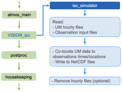
This section describes how our code is interfaced within the UM framework. The UM uses Rose configuration editor (Shin et al., 2018) and the Cylc workflow engine (Oliver et al., 2018), respectively, as a graphical user interface (GUI) and to control the model simulation workflow. Rose is a system for creating, editing, and running application configurations, and it is used as the GUI for the UM to configure input namelists. Cylc is a workflow engine that is used to schedule the various tasks needed to run an instance of the UM in the correct sequence: for example, atmos_main runs the main UM code, postproc deals with data formatting and archiving, and housekeeping deletes unnecessary files from the user workspace.
A new Rose application, VISION_iso, was created and inserted into the Cylc workflow between the model integration step (atmos_main) and the postproc step (see Fig. 1). This new application includes an input namelist and calls ISO_simulator.py; the NetCDF output files, containing model data co-located to the observations, are then sent to the MASS tape archive during the postproc step.
Since this software can be embedded into the UM runtime workflow and operates on UM output files (rather than being part of the UM source code), it has the following advantages compared to the approach in Telford et al. (2013):
-
Model data interpolated to the measurement times and locations is output using the internationally recognised NetCDF format, thus providing any required metadata information and making handling and analysis quicker and easier for users.
-
The code runs in parallel to the atmosphere model and does not affect the model run time.
-
The code can easily be customised to process any model data (not just UM data), therefore making it useful to the wider atmospheric science community.
Model data interpolated to the measurement times and locations can then be archived for long-term storage. When embedded into the UM workflow, data can either be transferred to the MASS tape archiving system or to the JASMIN data analysis facility (Lawrence et al., 2012). Further savings in data storage can be made by optionally deleting the hourly model output files used by the VISION toolkit.
Model simulations of UKESM were performed with a horizontal grid of 1.875° × 1.25° and 85 vertical levels with a model top at 85 km, and ERA reanalysis data were used to constrain the model meteorology (Telford et al., 2008) to allow better comparison with observations. For more information on the model configuration and details of the simulations, the reader is referred to the model description in Russo et al. (2023) and Archibald et al. (2024).
The aim of the plots in this section is not to answer specific science questions but to illustrate the way ISO_simulator can be used to co-locate model data onto different sets of in situ observations, namely ground-based stations, ships/buoys, sondes/flights, and unmanned aerial vehicles (UAVs).
All model data are output hourly from UKESM at a horizontal resolution of ∼150 km and then co-located, using ISO_simulator, to the same time and geographical coordinates as the observational data; the resulting data have the same time and spatial resolution as the observational data, making model data directly comparable to observational data. Furthermore, since the model and observational datasets can be compared over a long period of time, spanning several years, it is possible to sample seasonal and interannual variability, with better statistical sampling of extreme values. This type of comparison can greatly help to identify and improve model biases and to use models and observations in synergy to better understand atmospheric processes.
4.1 Cape Verde Atmospheric Observatory
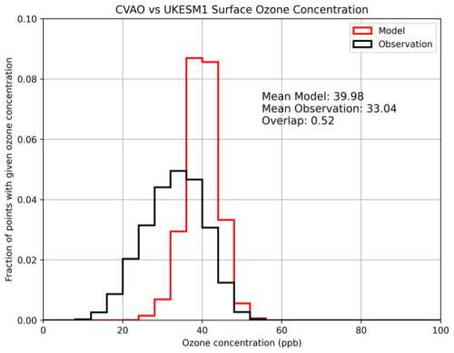
The Cape Verde Atmospheric Observatory (CVAO) provides long-term ground-based observations in the tropical North Atlantic Ocean region (16°51′49′′ N, 24°52′02′′ W). The CVAO is a Global Atmospheric Watch (GAW) station of the World Meteorological Organisation (WMO); measurements from CVAO are available in the UK Centre for Environmental Data Analysis (CEDA) data archives (http://catalogue.ceda.ac.uk/uuid/81693aad69409100b1b9a247b9ae75d5, last access: 8 January 2025; Carpenter et al., 2024). The University of York provides the CVAO trace gas measurements, supported by the Natural Environment Research Council (NERC) through the National Centre for Atmospheric Science (NCAS) Atmospheric Measurement and Observation Facility (AMOF). Data from CVAO were chosen as an example of surface station data because the ozone measurements are provided at a higher temporal resolution than the hourly model output; ISO_simulator can therefore be useful to interpolate model data in time to match the time of the observations.
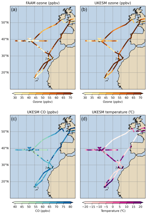
Figure 4FAAM and UKESM ozone concentrations (a, b); UKESM carbon monoxide and temperature (c, d). UKESM data are co-located in space and time to match the data collected during all FAAM flights in August 2019.
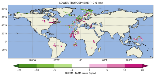
Figure 5Difference between UKESM and FAAM ozone concentrations (ppbv) in the lower troposphere (0–6 km) for all FAAM flights which measured ozone between 2010 and 2020.
4.2 Ships and buoys dataset
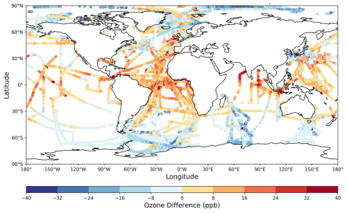
The Tropospheric Ozone Assessment Report (TOAR; https://igacproject.org/activities/TOAR/TOAR-II, last access: 8 January 2025) is an international activity under the International Global Atmospheric Chemistry project. It aims to assess the global distribution and trends of tropospheric ozone and to provide data that are useful for the analysis of ozone impacts on health, vegetation, and climate. A novel dataset has been produced by the TOAR “Ozone over the Oceans” working group. This dataset is an extension of previous similar datasets (Lelieveld et al., 2004; Kanaya et al., 2019), and it combines ship and buoy data from the 1970s to the present day. This dataset will be released later this year as part of the TOAR-II assessment; given the large temporal span, this dataset constitutes a great example of using ISO_simulator to compare model and observational data over a large number of years.
UKESM data were co-located to the same times and locations as observations. The plot in Fig. 3 shows the difference between modelled and observed ozone.
4.3 Aircraft data: comparison to FAAM and ATom
The FAAM Airborne Laboratory is a state-of-the-art research facility dedicated to the advancement of atmospheric science.
It operates a specially adapted BAe 146-301 research aircraft and is based at Cranfield University. The FAAM Airborne Laboratory is funded by the Natural Environment Research Council and managed through the National Centre for Atmospheric Science (NCAS).
FAAM data from 2010 to 2020 were processed to extract ozone, time, latitude, longitude, air pressure, and altitude and to ensure variable names were consistent throughout this time period (Russo et al., 2024). Figures 4 and 5 show comparisons of modelled data and ozone observed by the FAAM aircraft. Figure 4 shows FAAM ozone from all individual flights from a specific campaign occurring in August 2019 and a number of model variables interpolated on the FAAM flight tracks (ozone, carbon monoxide, and temperature). Figure 5 shows the difference between modelled and observed ozone for all flight points between the surface and ∼6 km and for all FAAM flights between 2010 and 2020.
The NASA Atmospheric Tomography (ATom) mission was a global-scale airborne campaign, funded through the NASA Earth Venture Suborbital-2 (EVS-2) programme, to study the impact of human-produced air pollution on greenhouse gases and on chemically reactive gases in the atmosphere. ATom utilised the fully instrumented NASA DC-8 research aircraft to measure a wide range of chemical and meteorological parameters in the remote troposphere (Thompson et al., 2022). Data from the ATom mission are available in the NASA data archive (https://doi.org/10.3334/ORNLDAAC/1925, Wofsy et al., 2021).
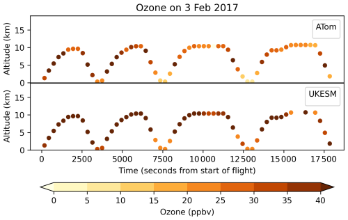
Figure 6 shows ozone concentrations from ATom and UKESM, as a function of time and altitude, for a specific flight on 3 February 2017.
The ability to sample atmospheric model output at the same time and location as in situ observations allows better synergy between model and observational data, resulting in better understanding of atmospheric processes and more effective model evaluation. However, doing this usually requires the processing of large volumes of high-frequency gridded model data. By interfacing with the CIS and cf-python libraries, we are able to efficiently automate this step, greatly reducing manual post-processing time and the volume of data that needs to be saved following a model simulation. This method is also transferable to many different atmospheric models, and the code is provided on GitHub under an open-source licence.
The use of the cf-python library to read-in the UM-format files significantly decreases the time taken to read these files when compared to the Iris or CIS libraries. This further reduces the time required for the HPC batch system to post-process the files from the global model to the times and locations of the in situ observations. An extension to this work is currently being carried out to be able to output model data on satellite swaths for better comparison between atmospheric models and satellite data.
The current version of the code presented in the article is available on GitHub (https://github.com/NCAS-VISION/VISION-toolkit, last access: 8 January 2025) and archived on Zenodo (https://doi.org/10.5281/zenodo.10927302, Russo and Bartholomew, 2024) under a BSD-3 licence.
Input data are available as follows:
-
Modelled ozone, https://catalogue.ceda.ac.uk/uuid/300046500aeb4af080337ff86ae8e776 (Abraham and Russo, 2024);
-
FAAM ozone dataset, https://catalogue.ceda.ac.uk/uuid/8df2e81dbfc2499983aa87781fb3fd5a (Facility for Airborne Atmospheric Measurements et al., 2024);
-
CVAO ozone dataset, https://catalogue.ceda.ac.uk/uuid/81693aad69409100b1b9a247b9ae75d5 (Carpenter et al., 2024);
-
ATom: Merged Atmospheric Chemistry, Trace Gases, and Aerosols, Version 2, https://doi.org/10.3334/ORNLDAAC/1925 (Wofsy et al., 2021).
MRR developed the ISO_simulator code and processed the 11-year FAAM ozone dataset. MRR and NLA performed the UKESM model simulations. MRR, AMM, and AJP performed data analysis and visualisation. NLA, EN, SLB, DH, and DWP supported the development of the ISO_simulator code. DAJS provided support with the FAAM data. NLA was the PI of the projects leading to the development of ISO_simulator, supported by MRR, SLB, and DH. MRR wrote the article with contributions from all co-authors.
The contact author has declared that none of the authors has any competing interests.
Publisher's note: Copernicus Publications remains neutral with regard to jurisdictional claims made in the text, published maps, institutional affiliations, or any other geographical representation in this paper. While Copernicus Publications makes every effort to include appropriate place names, the final responsibility lies with the authors.
This work was funded by the Natural Environment Research Council (NERC) under the embedded CSE programme of the ARCHER2 UK National Supercomputing Service (http://www.archer2.ac.uk, last access: 8 January 2025), hosted at the University of Edinburgh (ARCHER2-eCSE02-2). This work used Monsoon2, a collaborative high-performance computing facility funded by the Met Office and NERC; the ARCHER2 UK National Supercomputing Service; and JASMIN, the UK collaborative data analysis facility. Maria R. Russo, Nathan Luke Abraham, David Hassell, and Sadie L. Bartholomew are funded by the NERC VISION project, part of the NERC-TWINE programme.
We thank the Atmospheric Measurement and Observation Facility (AMOF), part of the National Centre for Atmospheric Science (NCAS), for providing the CVAO dataset. We thank all contributors to the TOAR ship and buoy ozone dataset (Yugo Kanaya, James Johnson, Kenneth Aikin, Alfonso Saiz-Lopez, Theodore Koenig, Suzie Molloy, Anoop Mahajan, and Junsu Gil). We thank the FAAM Airborne Laboratory for providing raw data input which was processed into the 11-year FAAM ozone dataset. We thank Ag Stephens and Wendy Garland from the Centre for Environmental Data Archival (CEDA) for technical support. We also thank Fiona O'Connor (UK Met Office) for suggesting the use of the CIS library. The local computer cluster (used for analysis in Table 2) was funded through the National Centre for Atmospheric Science Capital Fund.
This research has been supported by the Natural Environment Research Council (NERC) through eCSE (project ID: ARCHER2-eCSE02-02) and VISION (grant no. NE/Z503393/1).
This paper was edited by Jason Williams and reviewed by Gijs van den Oord, Thomas Clune, and Manuel Schlund.
Abraham, N. L. and Russo, M. R.: UKESM1 hourly modelled ozone for comparison to observations. NERC EDS Centre for Environmental Data Analysis [data set], https://catalogue.ceda.ac.uk/uuid/300046500aeb4af080337ff86ae8e776, last access: April 2024.
Anderson, D. C., Duncan, B. N., Fiore, A. M., Baublitz, C. B., Follette-Cook, M. B., Nicely, J. M., and Wolfe, G. M.: Spatial and temporal variability in the hydroxyl (OH) radical: understanding the role of large-scale climate features and their influence on OH through its dynamical and photochemical drivers, Atmos. Chem. Phys., 21, 6481–6508, https://doi.org/10.5194/acp-21-6481-2021, 2021.
Archibald, A. T., Sinha, B., Russo, M., Matthews, E., Squires, F., Abraham, N. L., Bauguitte, S., Bannan, T., Bell, T., Berry, D., Carpenter, L., Coe, H., Coward, A., Edwards, P., Feltham, D., Heard, D., Hopkins, J., Keeble, J., Kent, E. C., King, B., Lawrence, I. R., Lee, J., Macintosh, C. R., Megann, A., Moat, B. I., Read, K., Reed, C., Roberts, M., Schiemann, R., Schroeder, D., Smyth, T., Temple, L., Thamban, N., Whalley, L., Williams, S., Wu, H., and Yang, M.-X.: Data supporting the North Atlantic Climate System: Integrated Studies (ACSIS) programme, including atmospheric composition, oceanographic and sea ice observations (2016–2022) and output from ocean, atmosphere, land and sea-ice models (1950–2050), Earth Syst. Sci. Data Discuss. [preprint], https://doi.org/10.5194/essd-2023-405, in review, 2024.
Carpenter, L. J., Hopkins, J. R., Lewis, A. C., Neves, L. M., Moller, S., Pilling, M. J., Read, K. A., Young, T. D., and Lee, J. D.: Continuous Cape Verde Atmospheric Observatory Observations [data set], https://catalogue.ceda.ac.uk/uuid/81693aad69409100b1b9a247b9ae75d5, last access: April 2024.
Facility for Airborne Atmospheric Measurements, National Centre for Atmospheric Science, UK, Russo, M., and Abraham, N. L.: VISION: Collated subset of FAAM ozone data 2010 to 2020, NERC EDS Centre for Environmental Data Analysis [data set], https://catalogue.ceda.ac.uk/uuid/8df2e81dbfc2499983aa87781fb3fd5a/ (last access: April 2024), 2024.
Griffiths, P. T., Murray, L. T., Zeng, G., Shin, Y. M., Abraham, N. L., Archibald, A. T., Deushi, M., Emmons, L. K., Galbally, I. E., Hassler, B., Horowitz, L. W., Keeble, J., Liu, J., Moeini, O., Naik, V., O'Connor, F. M., Oshima, N., Tarasick, D., Tilmes, S., Turnock, S. T., Wild, O., Young, P. J., and Zanis, P.: Tropospheric ozone in CMIP6 simulations, Atmos. Chem. Phys., 21, 4187–4218, https://doi.org/10.5194/acp-21-4187-2021, 2021.
Hassell, D. and Bartholomew, S.: cfdm: A Python reference implementation of the CF data model, JOSS, 5, 2717, https://doi.org/10.21105/joss.02717, 2020.
Hattersley, R., Little, B., Peglar, P., Elson, P., Campbell, E., Killick, P., Blay, B., De Andrade, E. S., Lbdreyer, Dawson, A., Yeo, M., Comer, R., Bosley, C., Kirkham, D., Tkknight, Stephenworsley, Benfold, W., Kwilliams-Mo, Tv3141, Filipe, Elias, Gm-S, Leuprecht, A., Hoyer, S., Robinson, N., and Penn, J.: SciTools/iris: v3.7.0, Zenodo [code], https://doi.org/10.5281/ZENODO.595182, 2023.
Kanaya, Y., Miyazaki, K., Taketani, F., Miyakawa, T., Takashima, H., Komazaki, Y., Pan, X., Kato, S., Sudo, K., Sekiya, T., Inoue, J., Sato, K., and Oshima, K.: Ozone and carbon monoxide observations over open oceans on R/V Mirai from 67° S to 75° N during 2012 to 2017: testing global chemical reanalysis in terms of Arctic processes, low ozone levels at low latitudes, and pollution transport, Atmos. Chem. Phys., 19, 7233–7254, https://doi.org/10.5194/acp-19-7233-2019, 2019.
Kim, P. S., Jacob, D. J., Fisher, J. A., Travis, K., Yu, K., Zhu, L., Yantosca, R. M., Sulprizio, M. P., Jimenez, J. L., Campuzano-Jost, P., Froyd, K. D., Liao, J., Hair, J. W., Fenn, M. A., Butler, C. F., Wagner, N. L., Gordon, T. D., Welti, A., Wennberg, P. O., Crounse, J. D., St. Clair, J. M., Teng, A. P., Millet, D. B., Schwarz, J. P., Markovic, M. Z., and Perring, A. E.: Sources, seasonality, and trends of southeast US aerosol: an integrated analysis of surface, aircraft, and satellite observations with the GEOS-Chem chemical transport model, Atmos. Chem. Phys., 15, 10411–10433, https://doi.org/10.5194/acp-15-10411-2015, 2015.
Lawrence, B. N., Bennett, V., Churchill, J., Juckes, M., Kershaw, P., Oliver, P., Pritchard, M., and Stephens, A.: The JASMIN super-data-cluster, ARXIV [preprint], https://doi.org/10.48550/ARXIV.1204.3553, 2012.
Lelieveld, J., Van Aardenne, J., Fischer, H., De Reus, M., Williams, J., and Winkler, P.: Increasing Ozone over the Atlantic Ocean, Science, 304, 1483–1487, https://doi.org/10.1126/science.1096777, 2004.
Oliver, H. J., Shin, M., Fitzpatrick, B., Clark, A., Sanders, O., Valters, D., Smout-Day, K., Bartholomew, S., Prasanna Challuri, Matthews, D., Wales, S., Tomek Trzeciak, Kinoshita, B. P., Hatcher, R., Osprey, A., Reinecke, A., Williams, J., Jontyq, Coleman, T., Dix, M., and Pulo, K.: Cylc – a workflow engine, Zenodo [software], https://doi.org/10.5281/ZENODO.1208732, 2018.
Rew, R., Davis, G., Emmerson, S., Cormack, C., Caron, J., Pincus, R., Hartnett, E., Heimbigner, D., Appel, L., and Fisher, W.: Unidata NetCDF, UniData [data set], https://doi.org/10.5065/D6H70CW6, 1989.
Russo, M. R. and Bartholomew, S. L.: NCAS-VISION/VISION-toolkit: 1.0 (v1.0), Zenodo [code], https://doi.org/10.5281/zenodo.10927302, 2024.
Russo, M. R., Kerridge, B. J., Abraham, N. L., Keeble, J., Latter, B. G., Siddans, R., Weber, J., Griffiths, P. T., Pyle, J. A., and Archibald, A. T.: Seasonal, interannual and decadal variability of tropospheric ozone in the North Atlantic: comparison of UM-UKCA and remote sensing observations for 2005–2018, Atmos. Chem. Phys., 23, 6169–6196, https://doi.org/10.5194/acp-23-6169-2023, 2023.
Russo, M. R., Abraham, N. L., and FAAM Airborne Laboratory: FAAM ozone dataset 2010 to 2020. NERC EDS Centre for Environmental Data Analysis [data set], https://catalogue.ceda.ac.uk/uuid/8df2e81dbfc2499983aa87781fb3fd5a (last access: 8 January 2025), 2024.
Shin, M., Fitzpatrick, B., Clark, A., Sanders, O., Smout-Day, K., Whitehouse, S., Wardle, S., Matthews, D., Oxley, S., Valters, D., Mancell, J., Harry-Shepherd, Bartholomew, S., Oliver, H. J., Wales, S., Seddon, J., Osprey, A., Dix, M., and Sharp, R.: metomi/rose: Rose 2018.02.0, Zenodo [code], https://doi.org/10.5281/ZENODO.1168021, 2018.
Smith, M., Met Office, and Natural Environment Research Council: Facility for Airborne Atmospheric Measurements [data set], http://catalogue.ceda.ac.uk/uuid/affe775e8d8890a4556aec5bc4e0b45c (last access: 8 January 2025), 2024.
Stevenson, D. S., Zhao, A., Naik, V., O'Connor, F. M., Tilmes, S., Zeng, G., Murray, L. T., Collins, W. J., Griffiths, P. T., Shim, S., Horowitz, L. W., Sentman, L. T., and Emmons, L.: Trends in global tropospheric hydroxyl radical and methane lifetime since 1850 from AerChemMIP, Atmos. Chem. Phys., 20, 12905–12920, https://doi.org/10.5194/acp-20-12905-2020, 2020.
Telford, P. J., Braesicke, P., Morgenstern, O., and Pyle, J. A.: Technical Note: Description and assessment of a nudged version of the new dynamics Unified Model, Atmos. Chem. Phys., 8, 1701–1712, https://doi.org/10.5194/acp-8-1701-2008, 2008.
Telford, P. J., Abraham, N. L., Archibald, A. T., Braesicke, P., Dalvi, M., Morgenstern, O., O'Connor, F. M., Richards, N. A. D., and Pyle, J. A.: Implementation of the Fast-JX Photolysis scheme (v6.4) into the UKCA component of the MetUM chemistry-climate model (v7.3), Geosci. Model Dev., 6, 161–177, https://doi.org/10.5194/gmd-6-161-2013, 2013.
Thompson, C. R., Wofsy, S. C., Prather, M. J., Newman, P. A., Hanisco, T. F., Ryerson, T. B., Fahey, D. W., Apel, E. C., Brock, C. A., Brune, W. H., Froyd, K., Katich, J. M., Nicely, J. M., Peischl, J., Ray, E., Veres, P. R., Wang, S., Allen, H. M., Asher, E., Bian, H., Blake, D., Bourgeois, I., Budney, J., Bui, T. P., Butler, A., Campuzano-Jost, P., Chang, C., Chin, M., Commane, R., Correa, G., Crounse, J. D., Daube, B., Dibb, J. E., DiGangi, J. P., Diskin, G. S., Dollner, M., Elkins, J. W., Fiore, A. M., Flynn, C. M., Guo, H., Hall, S. R., Hannun, R. A., Hills, A., Hintsa, E. J., Hodzic, A., Hornbrook, R. S., Huey, L. G., Jimenez, J. L., Keeling, R. F., Kim, M. J., Kupc, A., Lacey, F., Lait, L. R., Lamarque, J.-F., Liu, J., McKain, K., Meinardi, S., Miller, D. O., Montzka, S. A., Moore, F. L., Morgan, E. J., Murphy, D. M., Murray, L. T., Nault, B. A., Neuman, J. A., Nguyen, L., Gonzalez, Y., Rollins, A., Rosenlof, K., Sargent, M., Schill, G., Schwarz, J. P., Clair, J. M. St., Steenrod, S. D., Stephens, B. B., Strahan, S. E., Strode, S. A., Sweeney, C., Thames, A. B., Ullmann, K., Wagner, N., Weber, R., Weinzierl, B., Wennberg, P. O., Williamson, C. J., Wolfe, G. M., and Zeng, L.: The NASA Atmospheric Tomography (ATom) Mission: Imaging the Chemistry of the Global Atmosphere, B. Am. Meteorol. Soc., 103, E761–E790, https://doi.org/10.1175/BAMS-D-20-0315.1, 2022.
Thornhill, G., Collins, W., Olivié, D., Skeie, R. B., Archibald, A., Bauer, S., Checa-Garcia, R., Fiedler, S., Folberth, G., Gjermundsen, A., Horowitz, L., Lamarque, J.-F., Michou, M., Mulcahy, J., Nabat, P., Naik, V., O'Connor, F. M., Paulot, F., Schulz, M., Scott, C. E., Séférian, R., Smith, C., Takemura, T., Tilmes, S., Tsigaridis, K., and Weber, J.: Climate-driven chemistry and aerosol feedbacks in CMIP6 Earth system models, Atmos. Chem. Phys., 21, 1105–1126, https://doi.org/10.5194/acp-21-1105-2021, 2021.
Wang, Y., Ma, Y.-F., Eskes, H., Inness, A., Flemming, J., and Brasseur, G. P.: Evaluation of the CAMS global atmospheric trace gas reanalysis 2003–2016 using aircraft campaign observations, Atmos. Chem. Phys., 20, 4493–4521, https://doi.org/10.5194/acp-20-4493-2020, 2020.
Watson-Parris, D., Schutgens, N., Cook, N., Kipling, Z., Kershaw, P., Gryspeerdt, E., Lawrence, B., and Stier, P.: Community Intercomparison Suite (CIS) v1.4.0: a tool for intercomparing models and observations, Geosci. Model Dev., 9, 3093–3110, https://doi.org/10.5194/gmd-9-3093-2016, 2016.
Wofsy, S. C., Afshar, S., Allen, H. M., Apel, E. C., Asher, E. C., Barletta, B., Bent, J., Bian, H., Biggs, B. C., Blake, D. R., Blake, N., Bourgeois, I., Brock, C. A., Brune, W. H., Budney, J. W., Bui, T. P., Butler, A., Campuzano-Jost, P., Chang, C. S., Chin, M., Commane, R., Correa, G., Crounse, J. D., Cullis, P. D., Daube, B. C., Day, D. A., Dean-Day, J. M., Dibb, J. E., DiGangi, J. P., Diskin, G. S., Dollner, M., Elkins, J. W., Erdesz, F., Fiore, A. M., Flynn, C. M., Froyd, K. D., Gesler, D. W., Hall, S. R., Hanisco, T. F., Hannun, R. A., Hills, A. J., Hintsa, E. J., Hoffman, A., Hornbrook, R. S., Huey, L. G., Hughes, S., Jimenez, J. L., Johnson, B. J., Katich, J. M., Keeling, R. F., Kim, M. J., Kupc, A., Lait, L. R., McKain, K., Mclaughlin, R. J., Meinardi, S., Miller, D. O., Montzka, S. A., Moore, F. L., Morgan, E. J., Murphy, D. M., Murray, L. T., Nault, B. A., Neuman, J. A., Newman, P. A., Nicely, J. M., Pan, X., Paplawsky, W., Peischl, J., Prather, M. J., Price, D. J., Ray, E. A., Reeves, J. M., Richardson, M., Rollins, A. W., Rosenlof, K. H., Ryerson, T. B., Scheuer, E., Schill, G. P., Schroder, J. C., Schwarz, J. P., St.Clair, J. M., Steenrod, S. D., Stephens, B. B., Strode, S. A., Sweeney, C., Tanner, D., Teng, A. P., Thames, A. B., Thompson, C. R., Ullmann, K., Veres, P. R., Wagner, N. L., Watt, A., Weber, R., Weinzierl, B. B., Wennberg, P. O., Williamson, C. J., Wilson, J. C., Wolfe, G. M., Woods, C. T., Zeng, L. H., and Vieznor, N.: ATom: Merged Atmospheric Chemistry, Trace Gases, and Aerosols, Version 2, ORNL DAAC, Oak Ridge, Tennessee, USA [data set], https://doi.org/10.3334/ORNLDAAC/1925, 2021.
Zeng, X., Atlas, R., Birk, R. J., Carr, F. H., Carrier, M. J., Cucurull, L., Hooke, W. H., Kalnay, E., Murtugudde, R., Posselt, D. J., Russell, J. L., Tyndall, D. P., Weller, R. A., and Zhang, F.: Use of Observing System Simulation Experiments in the United States, B. Am. Meteorol. Soc., 101, E1427–E1438, https://doi.org/10.1175/BAMS-D-19-0155.1, 2020.


