The DOE E3SM version 2.1: overview and assessment of the impacts of parameterized ocean submesoscales

The U.S. Department of Energy's Energy Exascale Earth System Model (E3SM) version 2.1 builds on E3SMv2 with several changes, with the most notable being the addition of the Fox-Kemper et al. (2011) mixed-layer eddy parameterization. This parameterization captures the effect of finite-amplitude, mixed-layer eddies as an overturning streamfunction and has the primary function of restratification. Herein, we outline the changes to the mean climate state of E3SM that were introduced by the addition of this parameterization. Overall, the presence of the submesoscale parameterization improves the fidelity of the v2.1 simulation by reducing the ocean surface biases in the North Atlantic present in v2, as illustrated by changes in the climatological sea surface temperature and salinity and the Arctic sea-ice extent. Other impacts include a slight shoaling of the mixed-layer depths in the North Atlantic and a small improvement in the Atlantic Meridional Overturning Circulation (AMOC). We note that the expected shoaling due to the parameterization is regionally dependent in our coupled configuration. In addition, we investigate why the parameterization and its impacts on mixed-layer depth have little impact on the simulated AMOC: despite increased dense-water formation in the Norwegian Sea, only a small fraction of the water formed makes its way south into the North Atlantic basin. Version 2.1 also exhibits small improvements in the atmospheric climatology, with smaller biases in many notable quantities and modes of variability.

1 Introduction

The U.S. Department of Energy (DOE) Energy Exascale Earth System Model (E3SM) aims to meet the energy mission and science needs of the DOE using state-of-the-art DOE computing resources. Version 1 (E3SMv1) was released in 2018, and while the land model and coupler were similar to those in CESM2 (Community Earth System Model; Hurrell et al., 2013; Danabasoglu et al., 2020), the river routing, ocean, sea ice, atmospheric physics, atmospheric dynamical core, and stratospheric chemistry were significantly different. Both lower-resolution (110 km atmosphere and 60–30 km ocean) and higher-resolution (25 km atmosphere and 18–6 km ocean) configurations were released (Golaz et al., 2019; Caldwell et al., 2019), as were biogeochemical and cryosphere configurations (Burrows et al., 2020; Comeau et al., 2022). Following version 1, version 2 (E3SMv2) was released in 2022 with significant improvements to the modeled climate, including a 2× speedup from E3SMv1 (Golaz et al., 2022). For this version, a lower-resolution configuration and a North American regionally refined configuration (Tang et al., 2023) have been released, with plans for a biogeochemistry configuration with interactive carbon and nutrient cycles and a cryosphere configuration with regional refinement over the Southern Ocean in the future.

Version 2.1 (E3SMv2.1) builds on E3SMv2 (Golaz et al., 2022) with several changes, most notably the addition of the so-called “Fox-Kemper2011” mixed-layer eddy (MLE) parameterization (hereafter referred to as FK11; Fox-Kemper et al., 2008, 2011). Shallow, ageostrophic baroclinic instabilities, often referred to as submesoscale instabilities, develop on lateral density fronts in the weakly stratified surface mixed layer. Once they become finite in amplitude, the resulting mixed-layer eddies slump the fronts, releasing potential energy and contributing to the restratification and shoaling of the mixed layer (Boccaletti et al., 2007). Due to their small spatial scales (𝒪(10 km)), these submesoscale instabilities and their effects are not explicitly resolved in global ocean models, even at “eddy-resolving” resolutions, and thus they need to be parameterized. Fox-Kemper et al. (2008) proposed a parameterization in the form of an overturning streamfunction to mimic the MLE fluxes of density and other tracers. By construction, this overturning streamfunction acts to slump isopycnals and enhance restratification of the mixed layer. This parameterization has been implemented in several other global ocean general circulation models, such as the Parallel Ocean Program (POP) model (Smith et al., 2010), the Modular Ocean Model (MOM) (Griffies, 2009; Adcroft et al., 2019), the Generalized Ocean Layered (GOLD) model (Adcroft and Hallberg, 2006), and the MIT General Circulation Model (MITgcm) (Marshall et al., 1997). According to Fox-Kemper et al. (2011), the general impacts of the parameterization within these models are the shoaling of the mixed layer (with the greatest effects being present in polar winter regions), a strengthening of the Atlantic Meridional Overturning Circulation (AMOC), a reduction in tracer ventilation, small changes to sea surface temperature (SST) and air–sea fluxes, and a reduction in sea-ice basal melting.

In this paper, we largely focus on documenting the implementation of the MLE parameterization from FK11 in the ocean component of the E3SM, the Model for Prediction Across Scales – Ocean (MPAS-Ocean). We investigate the response of the coupled model to the MLE fluxes, with a particular focus on high-latitude convection and large-scale ocean circulation, including the AMOC.

2 Methods

E3SMv2.1 implemented several changes from v2, including several bug fixes and additional options that are detailed in Appendix B. However, the primary notable difference from E3SMv2 is the inclusion of the FK11 MLE parameterization outlined below (Fox-Kemper et al., 2011). All other features listed in Appendix B are not active in the v2.1 configuration simulations used in this study, and any bug fixes were shown to have no significant climate-changing effects in testing; therefore, we will assume any changes from v2 to v2.1 are due to the addition of the FK11 MLE parameterization and any feedbacks it may induce in the model.

2.1 Mixed-layer eddy parameterization

The FK11 MLE parameterization captures finite-amplitude, mixed-layer eddies as an overturning streamfunction and has the primary function of restratification. It applies a submesoscale transport velocity through a streamfunction given as follows:

$$\begin{array}{}\text{(1)}& {\displaystyle }\mathrm{\Psi }=C_{\mathrm{e}}{\displaystyle \frac{{\mathrm{\Delta }}_{\mathrm{S}}}{L_f}}{\displaystyle \frac{H^{\mathrm{2}}\mathrm{\nabla }{\stackrel{\mathrm{‾}}{b}}^z\times \widehat{z}}{\sqrt{f^{\mathrm{2}}+{\mathit{\tau }}^{-\mathrm{2}}}}}\mathit{\mu }\left(z\right),\text{(2)}& {\displaystyle }\mathit{\mu }\left(z\right)=max\left\{\mathrm{0},\left[\mathrm{1}-{\left({\displaystyle \frac{\mathrm{2}z}{H}}+\mathrm{1}\right)}^{\mathrm{2}}\right]\left[\mathrm{1}+{\displaystyle \frac{\mathrm{5}}{\mathrm{21}}}{\left({\displaystyle \frac{\mathrm{2}z}{H}}+\mathrm{1}\right)}^{\mathrm{2}}\right]\right\},\text{(3)}& {\displaystyle }{L}_f=max\left(L_{f,\min },\left|{\mathrm{\nabla }}_H{\stackrel{\mathrm{‾}}{b}}^z\right|H/f^{\mathrm{2}},NH/\left|f\right|\right),\end{array}$$

where C_e is an efficiency coefficient, Δ_S is the local model grid scale dimension, H is the mixed-layer depth, ${\stackrel{\mathrm{‾}}{b}}^z$ is the depth-average buoyancy over the mixed layer, $\widehat{z}$ is the unit vertical vector, f is the Coriolis parameter, τ is the time needed to mix momentum across the mixed layer, L_f,min is a limiting value of L_f to guarantee stability (typically 0.2–5 km), and N is the buoyancy frequency. Equation (1) can be physically interpreted as an overturning streamfunction that produces a bolus velocity ($u_{\mathrm{MLE}}=\mathrm{\nabla }\times \mathrm{\Psi }$) that acts to slump fronts and provide MLE fluxes to tracers. Equation (2) can be interpreted as a structure function for the vertical fluxes that has a maximum in the middle of the mixed layer and vanishes to zero at the surface and beneath the mixed layer. Equation (3) can be interpreted as an estimate of the typical local width of mixed-layer fronts, which is set here in this model configuration as the mixed-layer deformation radius. While recent work has been done to improve the representation of L_f (Bodner et al., 2023), we use the original formulation from Fox-Kemper et al. (2011) in this study.

2.2 Model setup

In order to test the impact of the above changes, we will compare simulations from the E3SMv2 (Golaz et al., 2022) and E3SMv2.1 configurations. As with E3SMv1 and v2, we will focus on climate metrics within the standard resolution configuration, which consists of a 110 km resolution atmosphere, a 165 km resolution land, a 0.5° river-routing model, and a variable-resolution ocean and sea-ice mesh going from 60 km in the mid-latitudes to 30 km at the Equator and poles. Similarly, the vertical grid remains the same as E3SMv1 and v2, with 72 layers in the atmosphere (∼ 60 km top) and 60 layers in the ocean (10 m near-surface resolution). Just like v2, the ocean model uses the Gent–McWilliams (GM; Gent and McWilliams, 1990) and Redi parameterizations (Redi, 1982), to simulate mesoscale eddies, in addition to the MLE parameterization outlined above.

2.3 Simulations

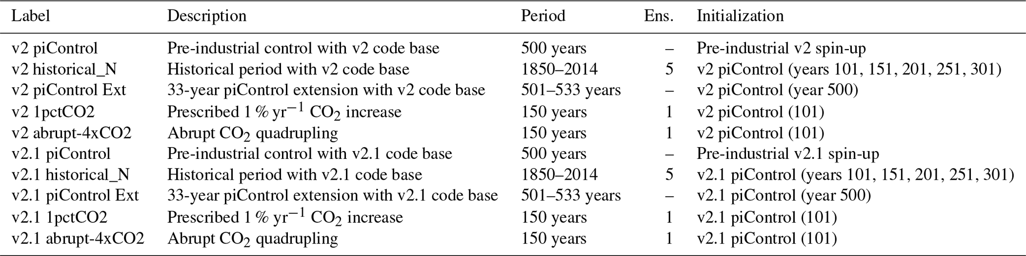
Table 1 summarizes the v2 and v2.1 simulations used in this paper. The full Diagnosis, Evaluation, and Characterization of Klima (DECK; Eyring et al., 2016); five historical simulations; and two idealized CO₂ simulations were run for each configuration. In addition, for the purposes of this paper and the investigation into the mechanisms of change due to the FK11 MLE parameterization, we ran an additional 33-year extension of both the v2 and v2.1 piControl simulations that included several passive tracers (details are provided in Sect. 4 below). Historical ensemble members (v2 historical_N and v2.1 historical_N) and the extension runs (v2 piControl Ext and v2.1 piControl Ext) were initialized from the v2 piControl and v2.1 piControl on 1 January of the year indicated in Table 1. Both the v2 and v2.1 simulations were completed on the DOE-E3SM owned “Chrysalis” machine, which is a traditional high-performance computer with 528 nodes with two AMD Epyc 7532 processors per node (64 cores per node) located at Argonne National Laboratory. Computational performance between the two configurations is comparable, with v2 and v2.1 producing 42 simulated years per day and 40.5 simulated years per day on average, respectively, on 105 nodes of Chrysalis.

Table 1 Summary of E3SMv2 and E3SMv2.1 simulations.

3 Overview of the v2.1 climate

In this section, we examine the climatological state of the v2.1 configuration. In particular, we focus on changes to the mean climate state of the North Atlantic that were introduced by the addition of the ocean MLE parameterization. For this purpose, we highlight the biases (with respect to observational estimates) in the context of the historical biases that were present in the v2 configuration.

3.1 Oceanic climate

For a global evaluation of relevant oceanic fields and a comparison between the v2 and v2.1 configurations, we first present spatiotemporal correlations (CORR) and root-mean-squared error (RMSE) relative to observations in Fig. 1. Annual ocean climatologies, correlations, and RMSE are constructed using the five-member v2 historical and v2.1 historical ensemble means over the 1980–2014 period. Observational data are drawn from merged Hadley Center-NOAA/OI data from 1870–2008 for SST (Hurrell et al., 2008), from the NASA Aquarius satellite from 2011–2015 for sea surface salinity (SSS) (Lagerloef et al., 2015), from merged absolute dynamic topography satellite data provided by AVISO (Archiving, Validation and Interpretation of Satellite Oceanographic data; processed by SSALTO/DUACS and distributed by AVISO+ (https://www.aviso.altimetry.fr, last access: 1 April 2018) with support from CNES) from 1992–2010 for sea surface height (SSH), from ARGO floats and the NCEI-NOASS World Ocean Database (WOD; Boyer et al., 2018) through the SEANOE data product from 1970-2021 for the mixed-layer depth (MLD) (de Boyer Montégut et al., 2004), and from Global Drifter Program drifters from 1979–2015 for near-surface eddy kinetic energy (EKE) (Laurindo et al., 2017).

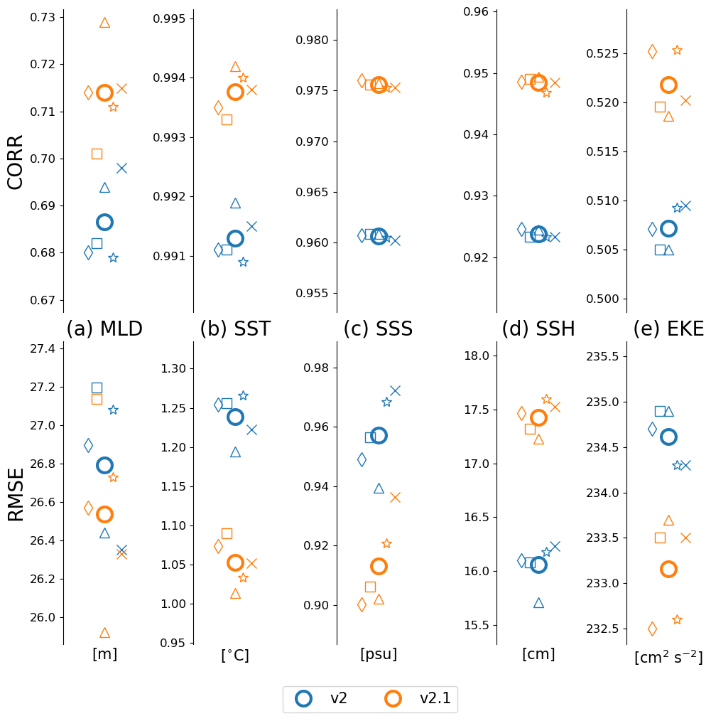
Figure 1 Correlations (top row) and RMSE (bottom row) of the global MLD (m), SST (°C), SSS (psu), SSH (cm), and EKE (kg² s⁻²) for the v2 (blue markers) and v2.1 (orange markers) historical ensemble simulations relative to observations (see Sect. 3.1 for data citations). Different symbols indicate the metric obtained from individual ensemble members and thick, open-circle markers indicate the multi-realization averages of the five v2 historical and v2.1 historical ensemble members over the 1980–2014 time period. Individual ensemble members have been spread out on the x axis to help with visualization of overlapping values.

Correlations serve to evaluate the model's ability to represent spatial patterns, while RMSE evaluate the model's representation of magnitude (although spatial patterns are also represented in RMSE) in comparison to observations. While modest, all correlation quantities increase across all ensemble members from the v2 to v2.1 configuration, indicating a better model representation of spatial patterns due to the presence of the MLE parameterization. For RMSE, although they are relatively modest, SST, SSS, and EKE see small global bias reductions going from the v2 to v2.1 configuration, and these reductions are seen across all ensemble members. While the mean MLD RMSE for the v2.1 configuration is slightly less than the v2 configuration, the ensemble spreads are essentially overlapping, indicating little difference between the two. Climatological maps of MLD biases discussed later in Fig. 5 indicate that the MLDs have changes in regional biases, where some regions see improvements and some see degradation going from the v2 to v2.1 configuration, and these changes compensate for each other when looking at this global RMSE metric.

There is an increase in the global SSH RMSE, which can be attributed to an initial ∼ 1.5–2 cm global increase in the first few years of the v2 piControl simulation that is not present in the v2.1 piControl simulation. This ∼ 1.5–2 cm offset remains throughout the v2 piControl simulation and each historical ensemble simulation. Plotting maps of global v2 historical and v2.1 historical climatological SSH (not shown) reveal this step decrease to be globally uniform going from the v2 to the v2.1 configuration, and time series comparing SSH anomalies from v2 and v2.1 shown in Fig. 2 show that the global anomaly ensemble spreads for the two different model versions essentially overlap throughout the historical simulations and have a similar trend over time to the observations. Taking this and the increased correlation metric for SSH (indicating better model SSH gradients) into account, we believe the v2.1 configuration does not exhibit an overall degraded global climatological SSH in comparison to the v2 configuration. In order to understand where each of the bias changes for MLD, SST, and SSS regionally occur, we next dive into a series of ocean climatological maps.

Figure 2 Time series of global SSH anomaly for the v2 configuration (black), v2.1 configuration (blue), and observations (orange). Thick lines denote the mean, while shading illustrates 1 standard deviation from that mean.

In the following, we present a series of ocean climatological maps where panel (a) is the v2 configuration bias in comparison to observations, panel (b) is the v2.1 configuration bias in comparison to observations, and panel (c) is the change in biases between the v2.1 and v2 configurations (i.e., positive (negative) values are an increase (decrease) in bias in the v2.1 quantity compared to v2). In these fields, we mask out values that are not considered statistically significant according to a one-sample t test (and a two-tailed critical value at α = 0.05) when comparing the model ensemble to observations and a two-sample t test when comparing the two model ensembles. Since most of the significant oceanic changes from v2 to v2.1 are within the North Atlantic and Arctic oceans, the figures here focus on those regions. Figures showing the full global ocean climatological biases are provided in Appendix A. The observational data used here are the same products used in the RMSE and correlation calculations of Fig. 1.

In general, the presence of the MLE parameterization improves the fidelity of the v2.1 configuration by reducing the North Atlantic Ocean surface biases present in v2 (Golaz et al., 2022), as illustrated by changes in the climatological SST (Fig. 3) and SSS (Fig. 4). A reduction in the v2 sea-ice biases is also seen and is discussed in Sect. 3.4.

Figure 3 Annual climatological SST biases (°C) with respect to observations for the (a) v2 and (b) v2.1 configurations. (c) The change in SST biases between the v2.1 and v2 configurations. Regions shaded in light gray denote where there are no data, while regions shaded in dark gray denote where the difference is not significant (according to a one-sample t test in a and b and a two-sample t test in c).

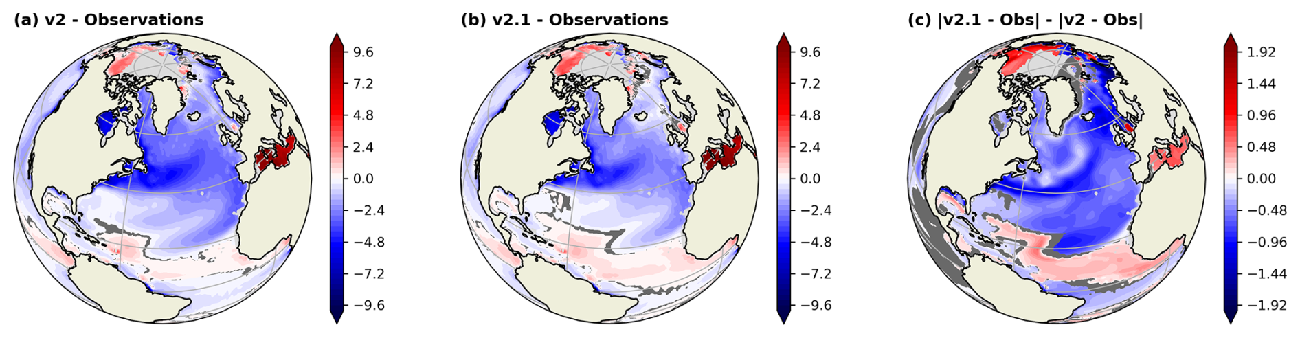
Figure 4 The same as Fig. 3 but for SSS (psu).

Looking in more detail at the SST field, Fig. 3 shows that although the v2.1 historical simulation ensemble retains large-scale SST biases (Fig. 3b) qualitatively similar to those of the v2 simulations (Fig. 3a) – namely a meridional dipole of excess heat in the South Atlantic and a cold bias in the North Atlantic – v2.1 presents a significant SST bias reduction (blue shading in Fig. 3c) that is focused primarily on the North Atlantic Subpolar Gyre, the Nordic Seas, and the Southern Ocean (see Figs. A1, A2, and A3 in Appendix A), reducing the temperature bias by 0.5–2 °C. Differences for all regions, including the Southern Ocean, can be found in Appendix A.

Likewise, the v2.1 historical simulation ensemble shows an improvement in the SSS bias in the North Atlantic, as shown by the blue region in Fig. 4c. The addition of the submesoscale parameterization is insufficient to fully mitigate the large-scale cold and fresh bias in the North Atlantic (still visible in blue in Figs. 3b and 4b) but leads to an improvement of 0.5–1 psu in the North Atlantic, including both the subtropical and subpolar gyres, and in the Nordic Seas. In the Barents, Kara, and Laptev seas, the bias reduction is even higher (1–2 psu). The v2.1 configuration and the presence of the MLE parameterization, however, do not appear to help the persistent salty SSS biases in the deep tropical North Atlantic, the Beaufort and Chukchi seas, and the Indian Ocean (see Appendix A).

MLDs do not show the same North Atlantic bias reduction as SST and SSS. In particular, the v2.1 historical simulation ensemble resulted in a slight shoaling of the mixed layer of approximately 20 m, increasing the bias over much of the North Atlantic (Fig. 5). This is most pronounced within the subpolar gyre, Nordic Seas, and eastern North Atlantic (red shading in Fig. 5c). This shoaling of the MLD is one of the primary effects of the FK11 MLE parameterization (Fox-Kemper et al., 2011). A localized decrease in MLD does occur in the vicinity of the Gulf Stream as the v2 deep biases there are significantly reduced.

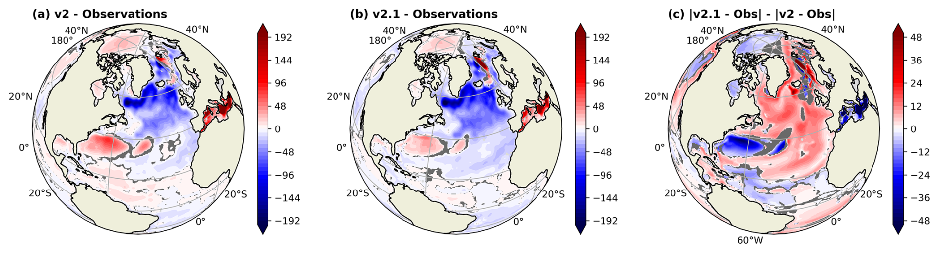
Figure 5 The same as Fig. 3 but for MLD (m).

A small uptick in the strength of the AMOC (Fig. 6) and a reduction in the variability (a noted effect of the FK11 MLE parameterization (Fox-Kemper et al., 2011)) are also seen. However, a larger increase in strength was expected given the reductions in the SST and SSS biases, which are likely responsible in part for reduced deep-water formation in the North Atlantic that should feed into the AMOC. We explore reasons for this difference in expected versus actual outcomes in Sect. 4. The bias differences in SSH or EKE are relatively small and not regionally focused but are instead somewhat uniform across the global oceans and are therefore not shown here.

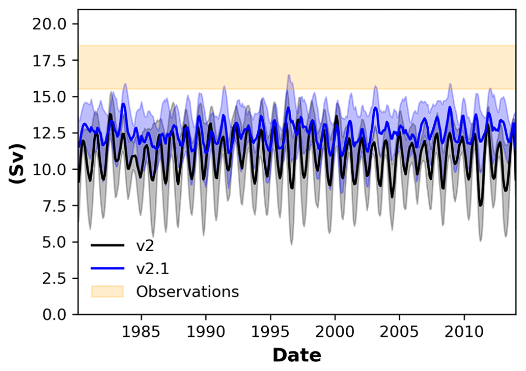
Figure 6 Time series of the maximum AMOC (Sv) at 26.5° N for the E3SM v2 configuration (black), the E3SM v2.1 configuration (blue), and an estimate of the observational range (orange) over the 1980–2014 period. Thick lines denote the ensemble mean, while shading illustrates 1 standard deviation from that mean after a 12-month smoothing is applied.

3.2 Atmospheric climate

For a collective evaluation of atmospheric fields and comparison of their performance between E3SMv2 and v2.1, we applied the Program for Climate Model Diagnosis and Intercomparison (PCMDI) Metrics Package (PMP; Lee et al., 2024), which is an open-source Python software package that provides quick-look objective comparisons of Earth system models with one another and with observations. In Fig. 7, model performances when reproducing observed global climatologies of multiple surface and upper-air fields are assessed, including precipitation, sea level pressure, radiation at the surface and the top of the atmosphere, air temperature at 200 and 850 hPa, surface air temperature, surface temperature, wind components at 200 and 850 hPa, and 500 hPa geopotential height. The spatiotemporal RMSE (Gleckler et al., 2008) was calculated, which is derived by getting a spatial RMSE of each calendar month of the climatological annual cycle and then averaging it across months. Although the differences are small, Fig. 7 indicates most fields in v2.1 have a reduced bias compared to v2. The improvement in surface temperature (ts) and near-surface air temperature (tas) is noticeable, which may be dominated by the improvement of the SST field, as shown in Fig. 3.

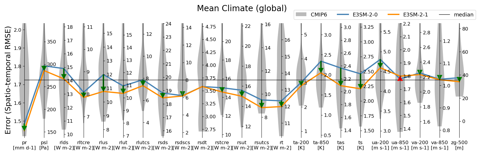
Figure 7 The PMP Parallel Coordinate Plot (Lee et al., 2024) for global mean climate evaluation, showing the spatiotemporal RMSE (Gleckler et al., 2008). Each vertical axis represents a different variable. Full names for model variables on the abscissa and their reference datasets can be found in Table 1 of Lee et al. (2024). RMSEs are constructed using the five v2 historical and v2.1 historical ensemble members over the 1981–2005 time period. Improvement (degradation) in E3SM v2.1 compared to E3SM v2 is highlighted as a downward green (upward red) arrow between lines. The midpoint of each vertical axis is shifted to represent the median result from the CMIP6 multi-model ensemble (horizontal black line), with the axis range stretched to the minimum and maximum from the median CMIP6 for visual consistency. The inter-model distributions of CMIP6 model performance are shown as shaded violin plots along each vertical axis. The first historical ensemble member of each model is used for the assessment.

3.3 Extratropical modes of variability

To examine the influence of the model update on the interannual climate variability modes, we applied the PMP's metrics for extratropical modes of variability (ETMoVs) for E3SMv2.1 and v2. Specifically, we have evaluated five atmospheric-based ETMoVs, including the Northern Annular Mode (NAM), North Atlantic Oscillation (NAO), Pacific–North America pattern (PNA), North Pacific Oscillation (NPO), and Southern Annular Mode (SAM), and two ETMoVs based on SST, i.e., the Pacific Decadal Oscillation (PDO) and the North Pacific Gyre Oscillation (NPGO). The atmospheric ETMoVs were evaluated for four seasons, while monthly time series were directly used for the SST-based modes. The Common Basis Function (CBF) approach is used to ensure a fair comparison of ETMoVs as simulated by climate models (Lee et al., 2019, 2021, 2024). The metric we selected for this study is the spatiotemporal RMSE obtained from the comparison of the model's CBF pattern to the observed empirical orthogonal functions (EOFs) pattern, which enables the inter-model comparison of bias magnitude that is from both the pattern and amplitude (Lee et al., 2019). To gauge the influence of internal variability on the evaluation process, we use the five v2 historical and v2.1 historical ensemble members. Metrics were calculated for each ensemble member of the model and then averaged across the five realizations. In Fig. 8, there are 14 metrics that show improvement, including NAM and NAO and eight cases of degradation. The ETMoV performance has not substantially changed in the context of the inter-model spread of CMIP6 models (shown as gray violin plots in the background). In summary, the large-scale extratropical modes of variability are not substantially different between E3SMv2 from v2.1.

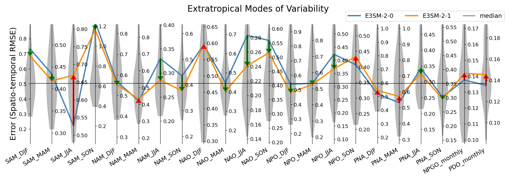
Figure 8 The PMP Parallel Coordinate Plot (Lee et al., 2024) for extratropical modes of variability evaluation, showing the spatiotemporal RMSE (Lee et al., 2019). Each vertical axis represents a different mode and season. Analysis is constructed using the five v2 historical and v2.1 historical ensemble members over the 1900–2005 time period. Improvement (degradation) in E3SMv2.1 compared to E3SMv2 is highlighted as a downward green (upward red) arrow between lines. Similar to Fig. 7, the middle of each vertical axis is set to the median of the group of benchmarking models (i.e., CMIP6), with the axis range stretched to the minimum or maximum from the median for visual consistency. The inter-model distributions of model performance are shown as shaded violin plots along each vertical axis.

3.4 Sea-ice climate

Similar to Sect. 3.1, in Figs. 9 and 10 we plot climatological means of sea-ice properties constructed using the five-member v2 historical and v2.1 historical ensemble means over the 1980–2014 period. Observational data are derived using measurements from multiple sensors across many satellite platforms detailed in Comiso (2017). Figure 9 shows an improvement in v2.1 Arctic sea-ice concentration, particularly around the Nordic Seas, Greenland, and the Labrador Sea (blue shading in Fig. 9c). Figure 10 shows a mix of improvement in the Indian Ocean and degradation in the Weddell, Amundsen, and Ross seas for v2.1 Antarctic sea-ice concentration.

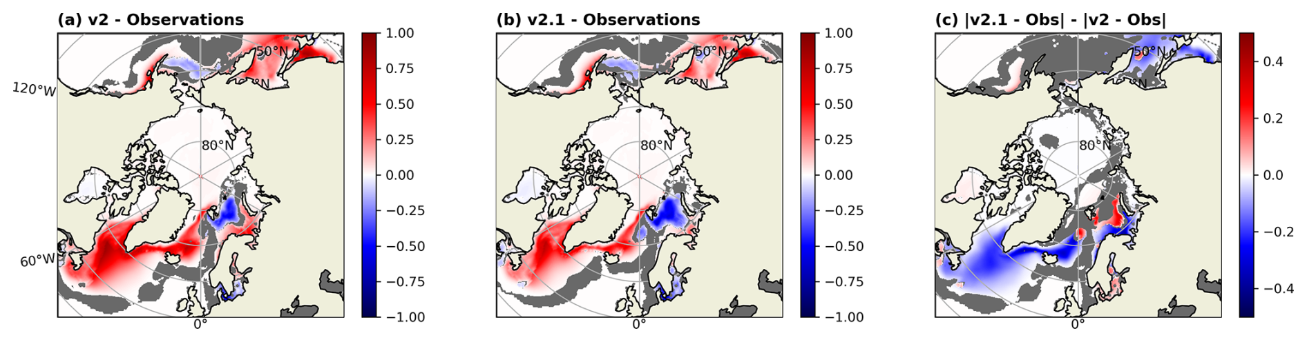
Figure 9 Annual climatological sea-ice concentration (fraction) biases with respect to observations in the Arctic for the (a) v2 and (b) v2.1 configurations. (c) Change in sea-ice concentration biases between v2.1 and v2 configurations. Regions shaded in dark gray denote where the difference is not significant (according to a one-sample t test in a and b and a two-sample t test in c).

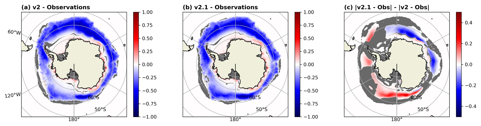
Figure 10 The same as Fig. 9 but for the Antarctic.

We evaluated the time mean and climatological annual cycle of sea-ice area in both the Arctic and Antarctic. In the calculation of the metric, we defined sea-ice area following Ivanova et al. (2016) as the area of grid cells with greater than 15 % sea-ice coverage (i.e., 15 % ice concentration) multiplied by their fraction of coverage and summed across grid cells within each region. For each of the Arctic and Antarctic regions, we partitioned the geographical region into three domains following Ivanova et al. (2016). The Arctic region is separated into the North Pacific, Central Arctic, and North Atlantic domains (shown in Fig. A5 in Appendix A), and the Antarctic region is separated to the South Atlantic, Indian Ocean, and South Pacific domains (shown in Fig. A6 in Appendix A). The model output is evaluated against the EUMETSAT OSI-SAF satellite-based product (OSI SAF, 2022). A date range of 1988–2014 was chosen for the maximal overlap between the v2 historical and v2.1 historical simulations and periods without missing data in the OSI-SAF product. The sea-ice area metrics that were proposed by Ivanova et al. (2016) and recently implemented in the PMP (Lee et al., 2024) are used for the analysis. We derived a simulated annual cycle and annual mean of the sea-ice area in each region for the time period of 1988–2014 to compare with observations (Fig. 11). The evaluation metrics are defined as mean square errors in the climatological annual cycle after removing the annual mean of the sea-ice area (Fig. 12). The overestimation of sea-ice area over the North Atlantic, North Pacific (mostly in December to May, Fig. 11), and Central Arctic (in August to September, Fig. 11) sub-regions and the underestimation in the Indian Ocean (in July to October, Fig. 11) sub-region in v2 are noticeably alleviated in v2.1, while the changes in other regions do not appear to be substantially different.

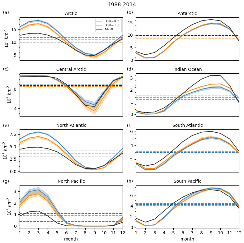
Figure 11 Climatological annual cycle (1988–2014) of total sea-ice area in the entire Arctic and its sub-regions (a, c, e, g) and the entire Antarctic and its sub-regions (b, d, f, h) obtained from the E3SMv2 (blue) and v2.1 (orange) simulations and the reference dataset EUMETSAT OSI-SAF (black line). Solid lines indicate the average of the five ensemble members, while the shaded color indicates the inter-ensemble spread. Dashed horizontal lines indicate the respective annual mean of the sea-ice area. In (b) the dashed blue line is hidden beneath the dashed orange line.

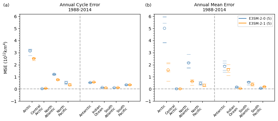
Figure 12 Mean square error (MSE) of the total sea-ice area annual cycle (annual mean removed; a) and annual mean (i.e., time mean bias squared; b) of each Arctic and Antarctic sub-region. Horizontal line markers indicate the metric obtained from individual ensemble members, while open circle markers indicate the multi-realization averages of the five ensemble members for each sub-region. Lower values are better. The vertical dashed gray line separates sub-regions of the Arctic (a) and Antarctic (b) in each panel. The diagnosed annual means and cycles for all regions and simulations and the reference dataset can be found in Fig. 11.

3.5 Climate sensitivity and transient climate response

We also performed two idealized CO₂ simulations (versions v2 and v2.1 of 1pctCO2 and versions v2 and v2.1 of abrupt-4xCO2) to estimate the model sensitivity to CO₂ forcing at different timescales. The equilibrium climate sensitivity (ECS) is defined as the equilibrium surface temperature change resulting from a doubling of CO₂ concentrations. ECS is typically approximated by linear regression of top-of-atmosphere radiation versus surface temperature in a 150-year “abrupt-4xCO2” simulation (Gregory et al., 2004), often referred to as “effective climate sensitivity”. Response on shorter timescales is measured by the transient climate response (TCR), which is defined as the change in surface temperature averaged for a 20-year period around the time of CO₂ doubling from a “1pctCO2” simulation. TCR depends on both climate sensitivity and ocean heat uptake rate.

ECS is nearly unchanged in E3SMv2.1 at 3.92 K compared to 4.0 K in E3SMv2. TCR is slightly smaller at 2.20 K compared to 2.41 K. Both values are substantially smaller than E3SMv1, which suffered from a high sensitivity (ECS of 5.30 K and TCR of 2.93 K; Golaz et al., 2019). Meehl et al. (2020) evaluated ECS and TCR for 37 CMIP6 models. They found that the multimodel mean ECS was 3.7 ± 1.1 K (standard deviation). The multimodel mean TCR was 2.0 ± 0.4 K. E3SMv2.1 is well within 1 standard deviation of the multimodel mean for both ECS and TCR but higher than the mean.

In the next section, we delve into the potential mechanisms for the changes in biases present in the North Atlantic Ocean and potential links between those biases and AMOC.

4 Relationship between AMOC and the state of the North Atlantic

In order to shed light on mechanisms creating these changes, in particular the relationship between AMOC and the North Atlantic biases, we examined several variables in detail. This was done in an effort to relate deep-water formation and overturning to surface biases. To do this, we primarily investigated tracer transports through the North Atlantic via a 33-year piControl extension run for both the v2 and v2.1 configurations (v2 piControl Ext and v2.1 piControl Ext) with three additional passive tracers. At year 501 of both the v2 and v2.1 piControl simulations, we added three passive tracers and ran the simulations out to year 533. The injection of one tracer was proportional to the sea-ice freshwater flux into and out of the ocean, the second tracer was set to one in the first grid layer globally at every time step, and the final tracer was set to one in the first grid layer at every time step but only within a North Atlantic latitude and longitudinal band of 50–80° N and 60° W–10° E, respectively. Conclusions from each of these tracers were roughly the same, and thus for clarity we only show and discuss the third tracer. For consistency between plots and analyses in this section, all figures and analyses utilize these v2 piControl Ext and v2.1 piControl Ext runs with passive tracers instead of the ensemble v2 historical and v2.1 historical runs utilized in the previous sections.

Figure 13 shows the annual climatological (a–b) MLD and (d–e) sea-ice concentrations in the Nordic Seas for the (a, d) v2 and (b, e) v2.1 configurations and changes in (c) MLD and (f) sea-ice concentration between the two configurations. The MLD and sea-ice concentration plots in Fig. 13 here differ from those in Figs. 5 and 9 in that Figs. 5 and 9 show (a, b) biases with respect to observations and (c) the change in biases with respect to observations, while Fig. 13 only shows (a, b, d, e) total MLD and sea-ice concentration and (c, f) the differences in total MLD and sea-ice concentration between the v2 and v2.1 configurations. Thus, the pattern and maximum differences in Figs. 5c, 9c, and 13c and f are not expected to be in exact agreement with each other.

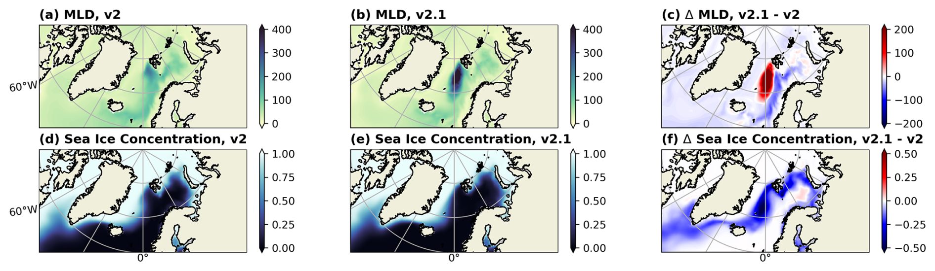
Figure 13 Annual climatological (a–b) MLD (m) and (d–e) sea-ice concentration (fraction) in the Nordic Seas for the (a, d) v2 and (b, e) v2.1 configurations. Change in (c) MLD and (f) sea-ice concentration between the v2.1 and v2 configurations.

While v2.1 showed slightly shallower MLDs than v2, both globally and in the subpolar gyre (outlined in the previous section), different patterns emerge in the Nordic Seas (Fig. 13a–c). In particular, we see a substantial deepening of the MLD by several hundred meters south of Svalbard and the Fram Strait in v2.1 compared with v2. A similar global shoaling and localized Nordic Seas deepening of the mixed layer was seen in both the Nucleus for European Modelling of the Ocean (NEMO) model (Calvert et al., 2020) and several coupled Earth system models in Fox-Kemper et al. (2011). Due to the emergence of this behavior only in fully coupled models and not in ocean-only models driven by normal year forcing, Fox-Kemper et al. (2011) attributed this response to air–sea and ice–sea feedback triggered by the MLE parameterization. In E3SM, while Northern Hemisphere sea-ice concentration is still too large in both model configurations, it was less so in v2.1 (Figs. 9 and 13d–e), resulting in a climatologically more open ocean in the Nordic Seas. Along with increased vertical mixing and surface fluxes within that same region (not shown), we speculate that similar air–sea and ice–sea feedbacks triggered by the MLE parameterization lead to the greater Nordic Seas MLDs in v2.1.

To further understand the effects of these feedbacks and deeper MLDs, we examined several passive tracers. Figure 14 shows the North Atlantic passive tracer (a–d) concentration for the v2.1 configuration at various depths and (e–h) the change in concentration between the v2.1 and v2 configurations at those same depths. Most notably, panels (d) and (h) show that tracer concentrations at depths greater than 1000 m within the Nordic Seas and along the edge of the Nansen Basin are much higher in the v2.1 configuration than the v2 configuration. Combined with enhanced MLDs and mixing and reduced sea-ice coverage in Nordic Seas, the v2.1 configuration appears to form significantly more deep, dense water in this region that is then exported into the Arctic. By forming more deep water here that is exported to depth by vertical mixing, the cold, fresh biases present at the surface in v2 are reduced in v2.1.

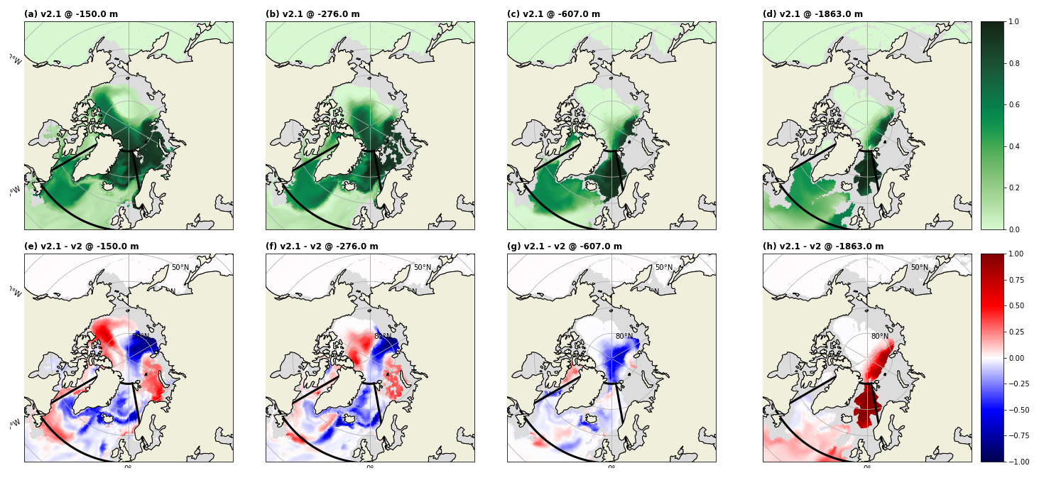
Figure 14 (a–d) Tracer concentration in the v2.1 configuration and (e–h) the change in concentration between the v2.1 and v2 configurations 33 years after tracer initiation at depths of (a, e) −150 m, (b, f) −276 m,(c, g) −607 m, and (d, h) −1863 m. Thick black boxes indicate the extent of the tracer surface forcing, while light gray shading denotes bottom topography at that model depth.

However, the vast majority of this extra deep water is exported to the Arctic via the North Atlantic Current flow through the Fram Strait (∼ 80 % of the released tracer is north of 75° N at the end of the 33 years in both v2 and v2.1). Very little ends up below 1000 m in the Atlantic, resulting in little change in the overturning circulation and providing a potential explanation for the lack of notable increase in the AMOC strength from v2 to v2.1. Figures 15 and 16 show changes in the winter and summer temperature and salinity along transects within the Labrador Sea and Nordic Seas between the v2 and v2.1 configurations. Within the Labrador Sea, where deep water is typically formed to feed the AMOC, we see very little change in the stratification structure between v2 and v2.1. A strong stratification buffer remains near the surface, preventing export of the cold, fresh water that remains there. Conversely, within the Nordic Seas, we see most of the interior stratification (below 1000 m) has been eroded away by the full-depth mixing associated with the deeper MLDs there. This full-depth mixing is present for most of the 500-year v2.1 piControl simulation and appears to have developed very early on in both the Greenland and Norwegian seas (see Fig. A4 in Appendix A). This lack of interior stratification and full-depth mixing allows for a greater connection of the surface to the deep, leading to greater export.

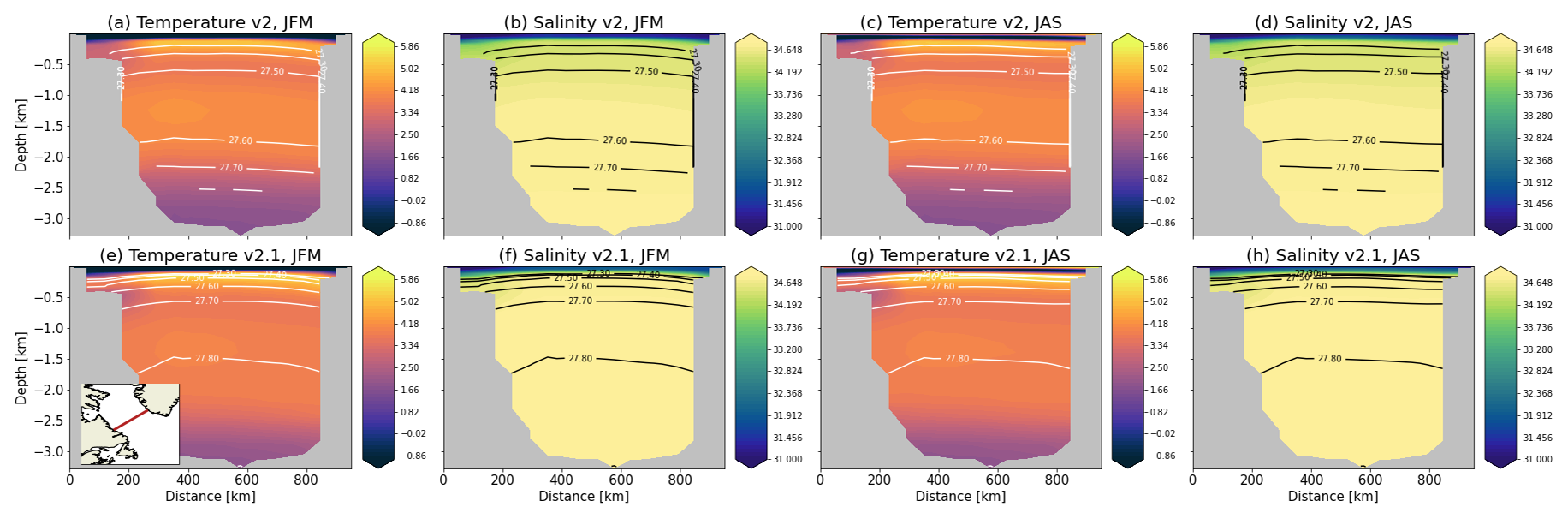
Figure 15 Annual climatological (a, c, e, g) temperature and (b, d, f, h) salinity in (a, b, e, f) winter (JFM) and (c, d, g, h) summer (JAS) for the v2 (a, b, c, d) and v2.1 (e, f, g, h) configurations across a Labrador Sea transect (the transect location is shown in the panel e inset). The black contour lines show select values of constant potential density.

Figure 16 The same as Fig. 15 but for a Nordic Seas transect.

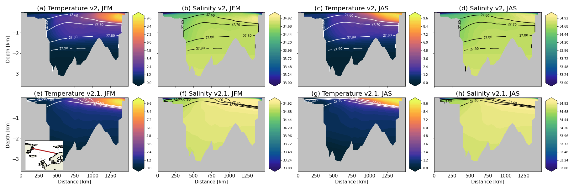
Figure 17 further examines the formation of this deep water by showing the surface water mass transformation in the North Atlantic basins for v2 (dotted line) and v2.1 (solid line) over the v2 piControl Ext and v2.1 piControl Ext runs. Surface water mass transformation diagnosed from surface heat and freshwater fluxes has been shown to vary with overturning strength in previous model comparison studies (Jackson and Petit, 2023; Petit et al., 2023). Here we diagnose surface water mass transformation by calculating surface buoyancy flux, excluding frazil ice formation, and area-integrating data over defined regions following Speer and Tziperman (1992). The diagnosed surface water mass transformation highlights a clear difference with the added MLE parameterization. In most regions of the North Atlantic and Nordic Seas, introducing the MLE parameterization in v2.1 leads to the formation of denser waters, either from an increase in the density of the waters formed (a shift to the right in Fig. 17) and/or from an increase in the water mass formation rate (visible as an increase in the peak value of the transformation rate). Specifically, the North Atlantic Ocean shows a transformation rate peak (18.2 Sv) in the v2.1 configuration that is similar in magnitude to that of v2 (18.4 Sv) but shifted to higher densities: the range of dense water formed (visible as a negative slope in transformation) is 26–27.2 kg m⁻³ instead of the lighter 25.6–27 kg m⁻³ range of formation in the v2 configuration. Similarly, the dense-water formation in the Norwegian Sea is shifted from 27.1–27.7 to 27.4–28 kg m⁻³ with the addition of the MLE parameterization (with its magnitude remaining at approximately 4 Sv across both configurations). In other regions, such as the Iceland Basin and Greenland Sea, both the peak transformation rate and the density range have increased in v2.1. In the Iceland Basin, the surface fluxes now form 2.4 Sv of dense water (27.2–27.6 kg m⁻³) instead of the weaker 1.5 Sv of slightly lighter waters (27–27.4 kg m⁻³) in v2. In the Greenland Sea, they form 1.4 Sv of dense water (27.9–28 kg m⁻³) compared to the 0.8 Sv of lighter waters (27.6–27.8 kg m⁻³) formed in v2 – a near doubling of dense-water formation in that region.

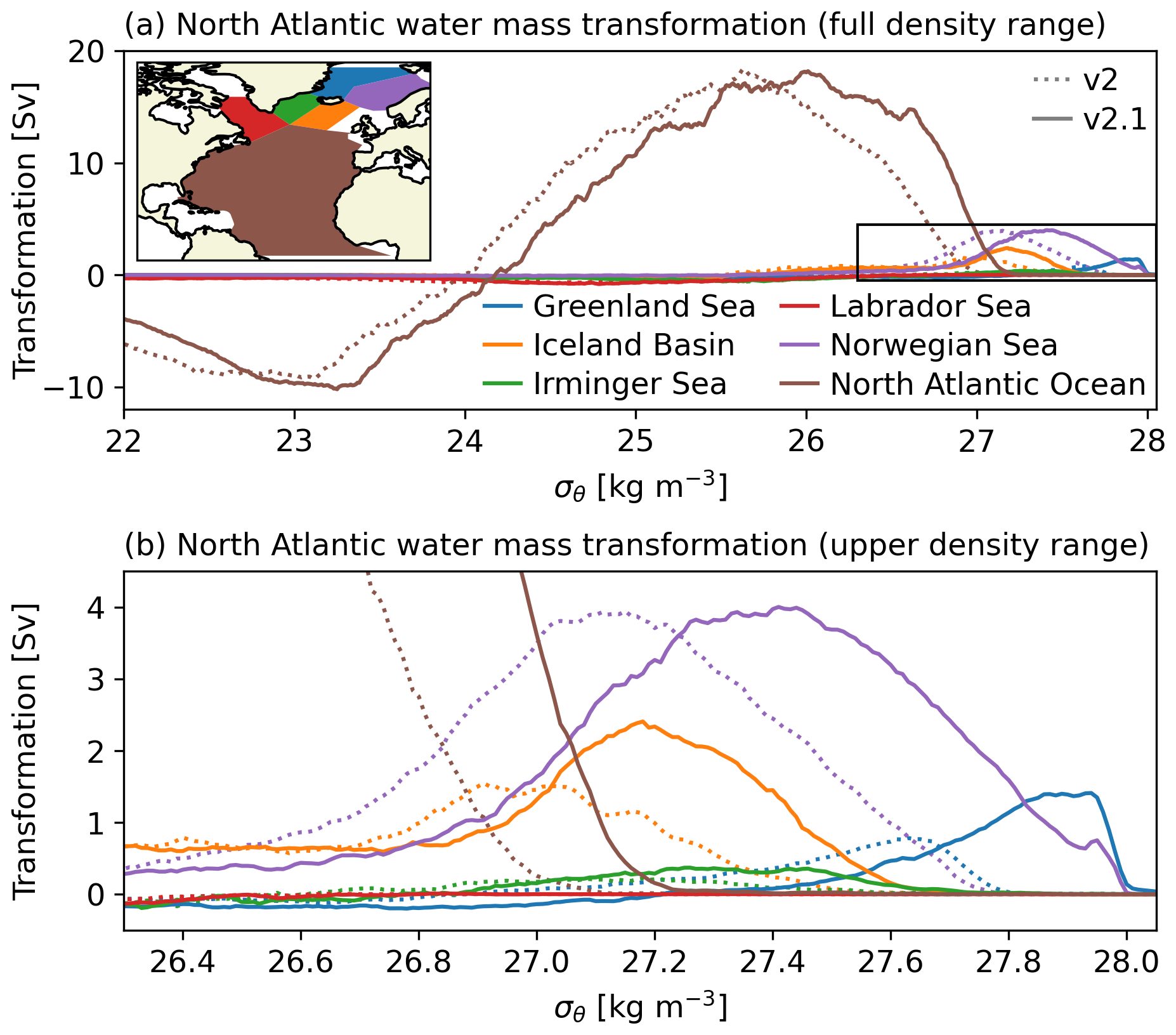
Figure 17 Surface water mass transformation in select North Atlantic basins in the v2.1 (solid lines) and v2 (dotted lines) configurations averaged over the 33-year piControl Ext runs (years 501–533). Panel (a) shows the full analyzed density range, while panel (b) zooms in on the higher density classes relevant to the subpolar basins shown. The extent of each region is shown in the map inset in panel (a). The x axis σ_θ is the surface-referenced potential density minus 1000 kg m⁻³. Transformation is calculated over a 0.01 kg m⁻³ density bin width, with a boxcar filter applied over a five-bin smoothing window to reduce noise.

In the Labrador and Irminger seas, the transformation rates and changes to transformation are small compared to the regions mentioned above. It is important to note that these last two regions are considered important sites of convection and dense-water mass formation in observations: convection in the Labrador Sea leads to important subpolar mode water formation, while deep-water formation in the Irminger Sea is considered a major contributor to Atlantic Deep Water, the AMOC (Petit et al., 2020), and possibly Labrador Sea Water (Pickart et al., 2003). Representing dense-water formation in climate models in the correct locations and appropriate magnitudes is an ongoing challenge, given that small-scale physical processes that contribute to it (e.g., convection and eddy mixing) are parameterized in models.

5 Conclusions

Overall, the v2.1 configuration resulted in some improvements to North Atlantic Ocean biases, particularly SST and SSS (Figs. 3 and 4), which resulted in improved sea-ice concentration in the North Atlantic (Fig. 9). Changes in MLD biases were as expected, mirroring FK11 with a general shoaling of the mixed layer (Fox-Kemper et al., 2011) visible in many regions (Fig. 5), although coupled feedbacks led to regional deepening of the MLD that reduced the mean MLD bias globally (Fig. 1). Additionally, although MLD is underestimated in comparison to observations in most regions, it does not appear to lead to any widespread degradation in the climate.

AMOC magnitude increased slightly with the addition of the MLE parameterization (Fig. 6). This is expected since the direct effect of the FK11 parameterization on AMOC appears to be model dependent and tends to either stabilize or minimally affect AMOC (Fox-Kemper et al., 2011). This effect holds for the v2.1 ensemble of simulations, which showed less variability in AMOC overall. Differences in AMOC may at least in part be due to a relocation of the site of deep convection from the Labrador and Irminger seas and North Atlantic to the Nordic Seas (Fox-Kemper et al., 2011). This hypothesis aligns with changes we saw in our modeled MLDs in v2.1 when compared with v2.

There appear to be differences in MLD in the Nordic Seas that are separate from the overall MLD shoaling created in v2.1, indicating potential changes in deep-water formation there (Fig. 13). Similar to Fox-Kemper et al. (2011), we also saw deep convection occurring in the Nordic Seas rather than in the Labrador and Irminger seas. Our water mass transformation analysis shows changes in deep-water formation, particularly in the North Atlantic and Norwegian Sea, with more dense water being formed in v2.1 than in v2 (Fig. 17). While it is not clear why this is the case, it does explain why our modeled AMOC improves slightly while not drastically altering the North Atlantic Subpolar Gyre. If increased deep-water formation was occurring in the Labrador and Irminger seas, we would expect to see a greater decrease in the SSS, SST, and sea-ice biases there. The passive tracer transport analysis in Sect. 4 for v2.1 indicates that the increased deep convection may not translate to a better AMOC because the dense water formed is transported northward into the Arctic rather than towards the south. Comparison of tracer advection from v2 to v2.1 shows deep northward convection from the Barents Sea into the Arctic in v2.1 (this does not occur in v2). Future work will attempt to elucidate the mechanisms behind this shift in deep-water formation.

Our results also indicate that the climatological characteristics of many surface and atmospheric fields in E3SMv2.1 have improved compared to v2 (Fig. 7). We have also examined the model performance of seven interannual extratropical modes of variability, including the atmospheric-based NAM, NAO, PNA, NPO, and SAM and two modes based on SST, i.e., the PDO and NPGO. Our results suggest noticeable improvement in the NAO and NAM; however, for most modes and seasons we find the large-scale extratropical modes of variability in E3SMv2.1 are not significantly different from v2 (Fig. 8). Orbe et al. (2020) distinguished the following two classes of model improvement: (1) “those that rely on a threshold of model representation that is crossed at a distinct moment in model development” and (2) “improvements that rely on more gradual, collective improvements in processes.” They argue that the performance evolution of extratropical modes of variability likely falls into the second category, e.g., due to enhancements in base climate representation and relevant processes, which might be evidenced via mixed influences across different modes and seasons. Additionally, the sample size available for this study limits any robust conclusions regarding performance changes in the simulation of extratropical modes of variability. Lastly, our analysis indicates that the TCR and ECS are essentially unchanged in E3SMv2.1 compared to v2.

Appendix A: Supplementary figures

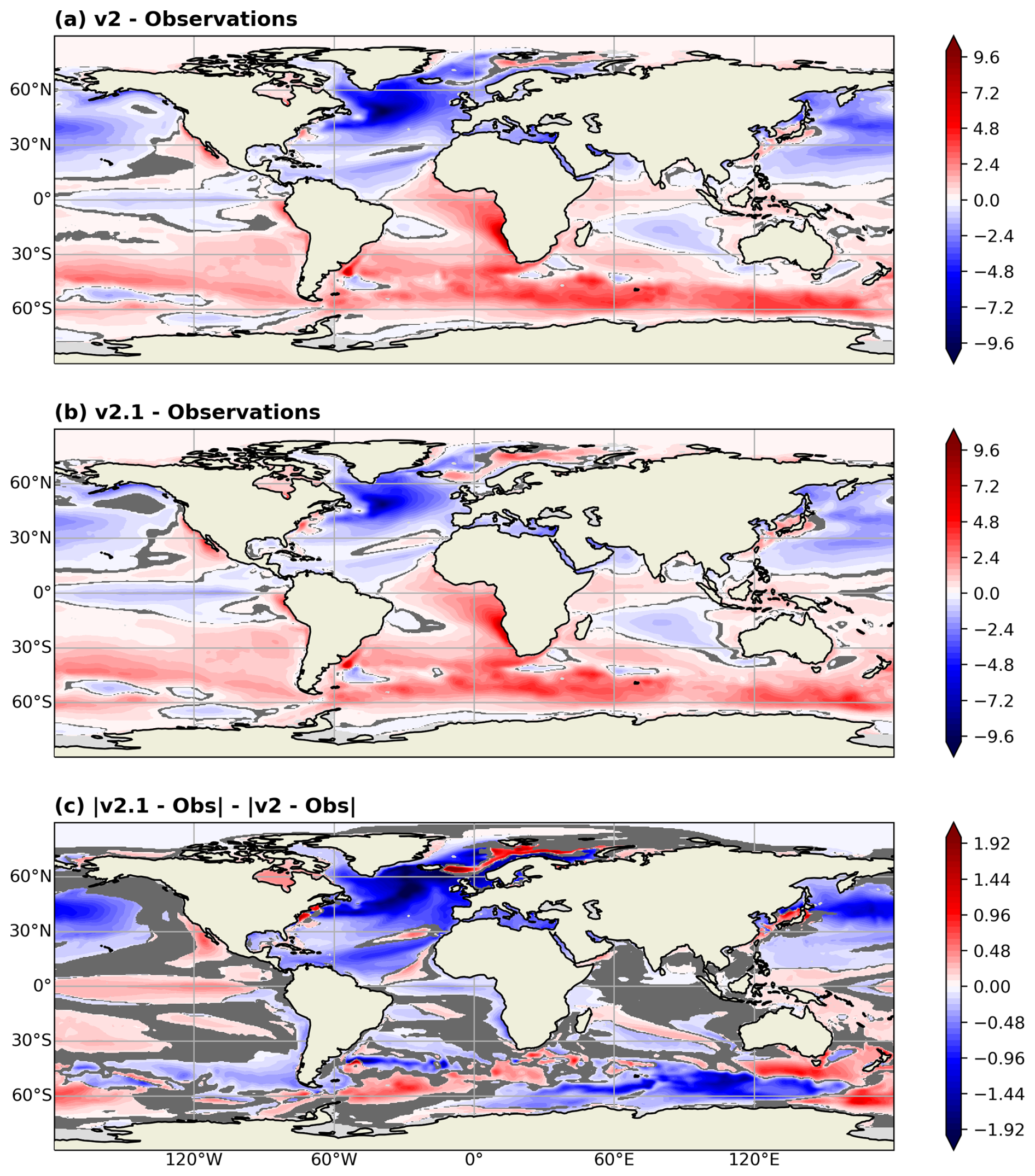
Figure A1 Global annual climatological SST biases (°C) with respect to observations for the (a) v2 and (b) v2.1 configurations. (c) Change in SST biases between v2.1 and v2 configurations. Regions shaded in light gray denote where there are no data, while regions shaded in dark gray denote where the difference is not significant (according to a one-sample t test in a and b and a two-sample t test in c).

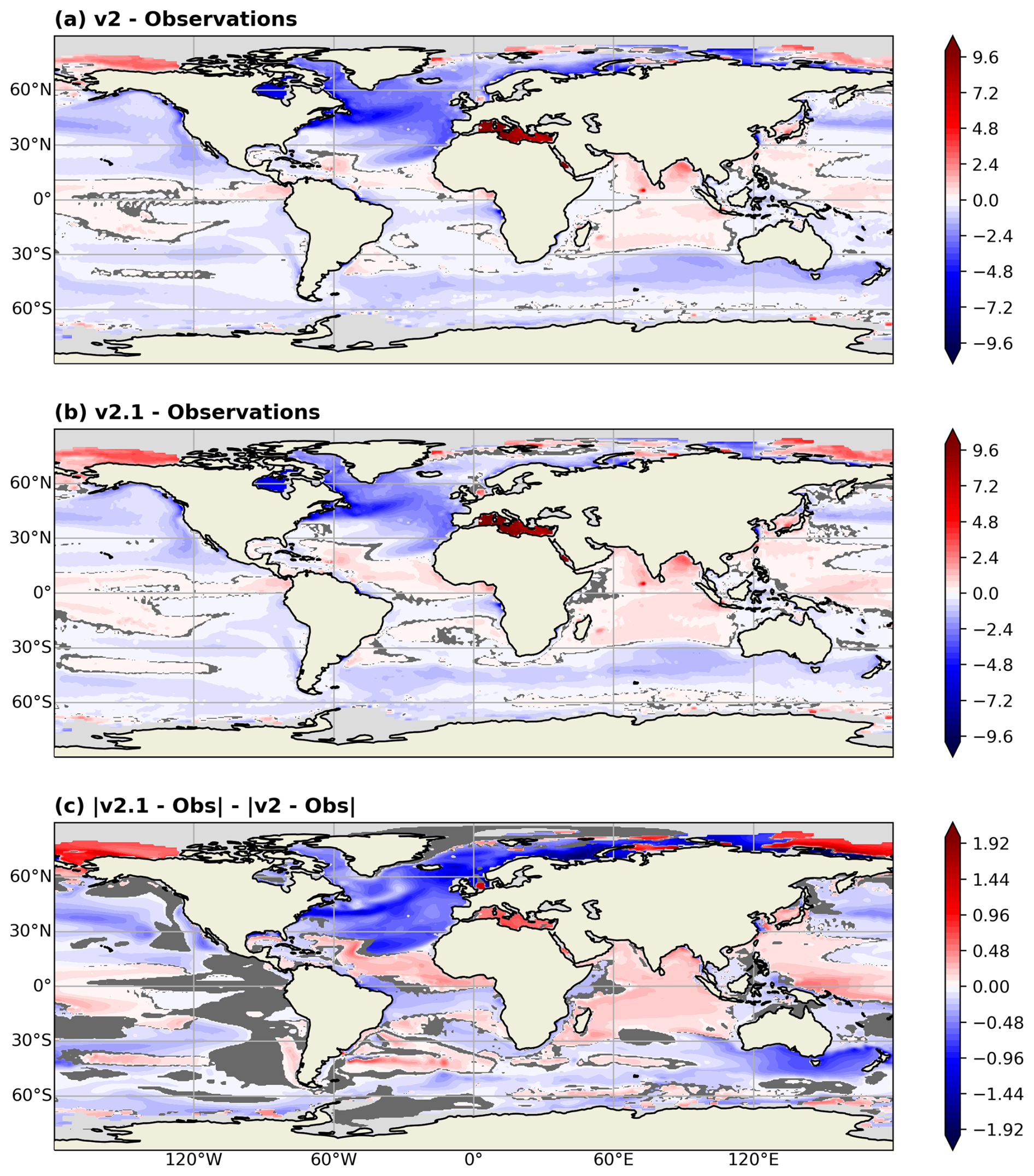
Figure A2 The same as Fig. A1 but for SSS (psu).

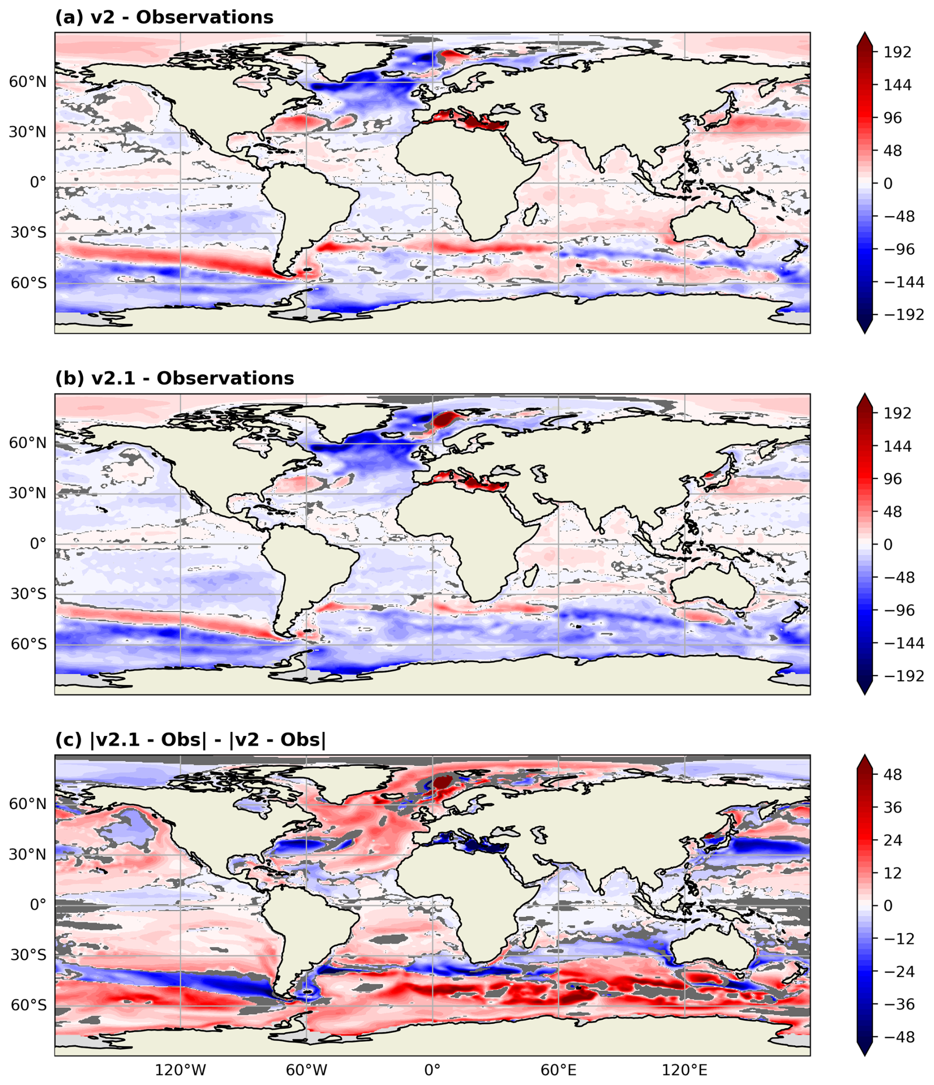
Figure A3 The same as Fig. A1 but for MLD (m).

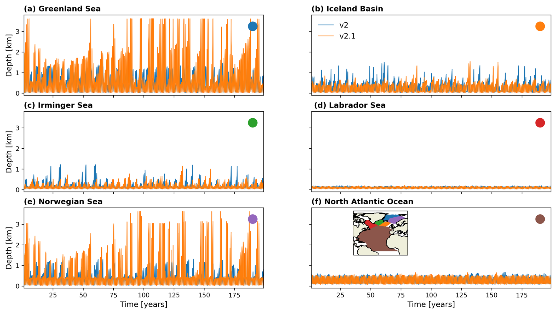
Figure A4 Maximum MLD (m) for the first 200 years of the v2 piControl (blue lines) and v2.1 piControl (orange lines) in the North Atlantic basins: (a) Greenland Sea, (b) Iceland Basin, (c) Irminger Sea, (d) Labrador Sea, (e) Norwegian Sea, and (f) North Atlantic Ocean. The scope of each region is shown in the map inset in panel (f), and these regions correspond to the regions used in Fig. 17.

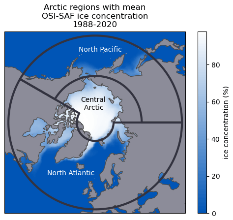
Figure A5 Partitioned Arctic geographical regions for the sea-ice area analysis in Sect. 3.4 and shown in Figs. 11 and 12 (Ivanova et al., 2016).

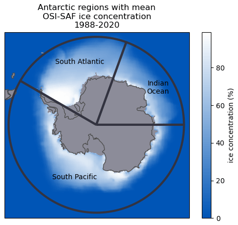
Figure A6 The same as Fig. A5 but for the Antarctic.

Appendix B: Code changes from v2 to v2.1

B1 Atmosphere

The atmosphere component of E3SM remains the E3SM Atmosphere Model (EAM). While there were no major changes in the default configuration of EAM from version 2, several new stealth features are included in the base code but were not active in the simulations analyzed in this study: a semi-Lagrangian tracer transport for theta-l dycore, a new algorithm for finding the tropopause, and new regionally refined mesh configurations.

B2 Ocean

The ocean component of E3SM remains MPAS-Ocean. Beyond the FK11 MLE parameterization discussed in detail in the main part of this paper, a correction for barotropic thickness consistency that reduces divergence noise was made and an ocean carbon conservation analysis member was added.

B3 Sea ice

The sea-ice component of E3SM remains MPAS-Seaice. From v2 to v2.1 a correction to how shortwave parameters are interpolated in the SNICAR-AD five-band radiation scheme was made, a sea-ice carbon conservation analysis member was added, the default sea-ice biogeochemistry namelist parameters were updated to be consistent with v2 improvements to nitrogen cycling, and a small bug fix in the ice–ocean dissolved organic nitrogen coupling was applied.

B4 Land

The land component of E3SM remains the E3SM Land Model (ELM). While there were no major changes in the default configuration of ELM, several optional stealth features have been added in the base code but were not active in the simulations analyzed in this study: an implementation of topography-based subgrid structure and accompanying parameterizations and atmospheric forcing downscaling; a new plant hydraulics scheme; two-way land–river hydrological coupling through the infiltration of floodplain water; an implementation of perennial crops; updates to the SNICAR-AD snow radiative transfer model; and an implementation of soil erosion and sediment yield in ELM-Erosion.

B5 River

The river component of E3SM remains the Model for Scale Adaptive River Transport (MOSART). While there were no major changes in the default configuration of MOSART, an optional stealth feature of two-way river–ocean hydrological coupling between MOSART and MPAS-Ocean was added to the base code but was not active in the simulations analyzed in this study.

B6 Coupled system

The coupler in E3SM remains cpl7 (Craig et al., 2012). Small bug fixes were applied to the land–atmosphere fluxes and the zenith angle calculation, and the option to calculate carbon budgets when heat and water budgets are active was added.