sedInterFoam 1.0: a three-phase numerical model for sediment transport applications with free surfaces

In this paper, an Eulerian two-phase flow model, sedFoam, is extended to include an air phase together with its water and sediment phases. The numerical model called sedInterFoam is implemented using the open-source library OpenFOAM. sedInterFoam includes the previous features of sedFoam for sediment transport modeling and also solves the air–water interface using the volume-of-fluid method coupled with the waves2Foam toolbox for free-surface wave generation and absorption. Using sedInterFoam, four test cases are successfully reproduced to validate the free-surface evolution algorithm's implementation, mass conservation of sediment and fluid phases, and predictive capabilities and to demonstrate its potential in modeling a broader range of coastal applications with sediment transport dominated by surface waves.

1 Introduction

Sediment transport is the main driver of morphological changes in coastal and fluvial environments (Sherwood et al., 2022). Understanding and modeling the physical processes involved in the movement of sediment particles forced by free-surface flow is a major issue. Accounting for and integrating the complex mechanisms involved in sediment transport in numerical models, e.g., interactions between solid particles and fluid turbulence, intergranular interactions, and surface-wave-driven processes, is a critical step in improving and enhancing existing model capabilities.

In the conventional single-phase modeling approach, Navier–Stokes equations are only solved for the fluid phase, sediment transport is related to the bottom shear stress using bed-load and suspended-load formulations, and the resulting morphological evolution is calculated using the Exner equation (Jacobsen and Fredsøe, 2014; Baykal et al., 2017). This modeling methodology has several limitations, although it is widely used because of its simplicity and computational efficiency. One of the major limitations is related to the empirical relation between horizontal and vertical sediment fluxes and the bottom shear stress. Indeed, most of these relations are valid for steady or mild transient flows and relatively coarse sediments in a controlled laboratory environment. As a result, a large discrepancy is observed between predicted and measured sediment fluxes for a given wave time series (Yu et al., 2012; van der A et al., 2013), suggesting that sediment flux solely parameterized by bottom shear stress is incomplete. Another major limitation of a conventional single-phase model is its inability to simulate the onset of scour due to piping (Sumer et al., 2001), which involves gap formation and tunneling due to seepage flow driven by an upstream–downstream pressure gradient.

To overcome these limitations, the Eulerian two-phase modeling approach which encompasses most of the physical mechanisms involved in the coupling between water and particles has been actively developed in the last 2 decades (Dong and Zhang, 2002; Hsu et al., 2004; Amoudry, 2014; Lee et al., 2016; Chauchat and Guillou, 2008; Chauchat, 2018; Mathieu et al., 2021). In the Eulerian two-phase flow approach, both the carrier phase and the dispersed sediment phase composed of the particles are seen as interpenetrating continua. Coupling between the two phases is modeled using spatially averaged interaction forces between the fluid and the particles (e.g., buoyancy, drag, or added mass), and particle–particle interactions can be included in the solid-phase stress closure models. As demonstrated in Tsai et al. (2022), an Eulerian two-phase model is able to simulate scour onset underneath a 2D pipeline due to seepage flow driven by an upstream–downstream pressure difference.

To make the scientific community benefit from the Eulerian two-phase model for sediment transport applications, an open-source solver called sedFoam (Chauchat et al., 2017; Cheng et al., 2017) implemented using the CFD library OpenFOAM (Jasak and Uroić, 2020) has been developed. The solver includes the most recent developments for intergranular stress modeling, e.g., the kinetic theory for granular flows (Chassagne et al., 2023), the μ(I) rheology (Boyer et al., 2011), turbulence closure models such as mixing length (Revil-Baudard and Chauchat, 2013), k−ε (Hsu et al., 2004), k−ω (Amoudry, 2014; Nagel et al., 2020), and large-eddy simulation models (Mathieu et al., 2021). sedFoam has been validated using many benchmarks (Chauchat et al., 2017) and successfully applied to various practical configurations, e.g., scour applications (Mathieu et al., 2019; Nagel et al., 2020; Tsai et al., 2022), ripple migration and geometry evolution (Salimi-Tarazouj et al., 2021a, b), sheet flow in an oscillatory boundary layer (Delisle et al., 2022; Mathieu et al., 2022), and immersed granular avalanches (Montellà et al., 2021, 2023).

Although two-phase flow models allowed us to significantly improve our knowledge of sediment transport processes in coastal and fluvial environments, this kind of modeling methodology is only applicable for configurations where free-surface effects are negligible or under simplifying assumptions, such as sediment transport in an oscillating water tunnel rather than under surface waves. Indeed, it is critical to include the ability to solve the propagation and breaking of surface waves in order to reproduce more realistic cross-shore sediment transport and morphodynamics that include the swash zone. To do so, resolving a third separated gaseous phase and implementing a numerical algorithm to resolve the evolution of the free surface is necessary. Kim et al. (2018) were the first to tackle this problem by combining an early version of sedFoam, the free-surface solver interFoam (Klostermann et al., 2013), and a library to generate free-surface waves (waves2Foam) (Jacobsen et al., 2012). With their solver, they successfully predicted sheet flow under monochromatic non-breaking waves by comparing numerical results with experimental data from Dohmen-Janssen and Hanes (2002) and studying sheet flow near a sandbar under near-breaking surface waves (Kim et al., 2019, 2021). However, the numerical implementation of the model prevented the sediment from being present in the air phase and, as a consequence, the sediment bed had to be located far away from the free surface. Despite the significant advances made possible by adding a third gaseous phase to their model, this limitation prevented simulation of configurations for which there were strong interactions between air, water, and sediment, such as in the swash zone. More recently, Lee et al. (2019) proposed a three-phase model similar to the one presented by Kim et al. (2018) using an equivalent but more general set of equations that allows sediment in both the air and water phases.

To provide an open-source model for nearshore sediment transport applications, the purpose of this work is to present and validate the open-source solver sedInterFoam, an extension of the two-phase model sedFoam for simulating sediment transport with a free surface and for intense interactions in the swash zone. Benefiting from the earlier work of Kim et al. (2018) in combining sedFoam, interFoam, and the wave generation library waves2Foam with the set of equations proposed by Lee et al. (2019), sedInterFoam is able to simulate configurations for which sediment is present in both air and water. The model is first presented in Sect. 2. Then, the model implementation and the solution algorithm are detailed in Sect. 3. In Sect. 4, the model is validated using benchmarks and applied to configurations related to cross-shore sediment transport and beach profile evolution.

2 Mathematical model

In the three-phase flow solver sedInterFoam, mass and momentum conservation equations are solved for the dispersed phase representing solid particles and the fluid phase constituted of the separated gas (air) and liquid (water) phases. The mass conservation equations for the solid, liquid, and gas phases are given by

$$\begin{array}{}\text{(1)}& {\displaystyle \frac{\partial \mathit{\varphi }}{\partial t}}+{\displaystyle \frac{\partial }{\partial x_i}}\left[\mathit{\varphi }{u}_i^{\mathrm{s}}\right]=\mathrm{0},\text{(2)}& {\displaystyle \frac{\partial }{\partial t}}\left[\mathit{\gamma }(\mathrm{1}-\mathit{\varphi })\right]+{\displaystyle \frac{\partial }{\partial x_i}}\left[\mathit{\gamma }(\mathrm{1}-\mathit{\varphi })u_i^{\mathrm{l}}\right]=\mathrm{0},\text{(3)}& {\displaystyle \frac{\partial }{\partial t}}\left[(\mathrm{1}-\mathit{\gamma })(\mathrm{1}-\mathit{\varphi })\right]+{\displaystyle \frac{\partial }{\partial x_i}}\left[(\mathrm{1}-\mathit{\gamma })(\mathrm{1}-\mathit{\varphi })u_i^{\mathrm{g}}\right]=\mathrm{0},\end{array}$$

with ϕ the sediment volume concentration; $u_i^{\mathrm{s}}$, $u_i^{\mathrm{l}}$, and $u_i^{\mathrm{g}}$ the solid-, liquid-, and gas-phase velocities, respectively; x_i the position vector with $i=\mathrm{1},\mathrm{2},\mathrm{3}$ representing the three spatial components; and γ the fluid indicator function defined as the ratio between the volume occupied by water and the total volume occupied by air and water in a cell (γ=1 in water, γ=0 in air, and $\mathrm{0}<\mathit{\gamma }<\mathrm{1}$ at the interface). γ is also commonly referred to as the volume of the fluid (Hirt and Nichols, 1981).

Instead of solving the three mass conservation equations, mass conservation can be fully accounted for by solving the conservation equations for ϕ and γ. Combining Eqs. (1), (2), and (3) and assuming $u_i^{\mathrm{l}}=u_i^{\mathrm{g}}$ at the interface because of the no-slip boundary condition for velocities between air and water, we obtain the conservation equation for the indicator function γ following

$$\begin{array}{}\text{(4)}& {\displaystyle \frac{\partial \mathit{\gamma }}{\partial t}}+{\displaystyle \frac{\partial }{\partial x_i}}\left[\mathit{\gamma }{u}_i^{\mathrm{f}}\right]-\mathit{\gamma }{\displaystyle \frac{\partial u_i^{\mathrm{f}}}{\partial x_i}}=\mathrm{0},\end{array}$$

with $u_i^{\mathrm{f}}=\mathit{\gamma }{u}_i^{\mathrm{l}}+(\mathrm{1}-\mathit{\gamma })u_i^{\mathrm{g}}$ representing the velocity of the fluid phase constituted of the air and water. More details about the derivation of Eq. (4) can be found in Appendix A.

Similarly, instead of solving momentum conservation equations for the three phases, the air and water mixture is considered a single fluid with varying densities and viscosities across the interface. The momentum conservation equations for the solid and fluid phases are given by

$$\begin{array}{}\text{(5)}& {\displaystyle }\begin{array}{rl}{\displaystyle \frac{\partial }{\partial t}}& {\displaystyle }\left[{\mathit{\rho }}^{\mathrm{s}}\mathit{\varphi }{u}_i^{\mathrm{s}}\right]+{\displaystyle \frac{\partial }{\partial x_i}}\left[{\mathit{\rho }}^{\mathrm{s}}\mathit{\varphi }{u}_i^{\mathrm{s}}{u}_j^{\mathrm{s}}\right]=\\ {\displaystyle }& {\displaystyle \frac{\partial }{\partial x_i}}{\mathrm{\Sigma }}_{ij}^{\mathrm{s}}+\mathit{\varphi }{\mathit{\rho }}^{\mathrm{s}}{g}_i+\mathit{\varphi }{f}_i+M_i,\end{array}\text{(6)}& {\displaystyle }\begin{array}{rl}{\displaystyle \frac{\partial }{\partial t}}& {\displaystyle }\left[{\mathit{\rho }}^{\mathrm{f}}(\mathrm{1}-\mathit{\varphi })u_i^{\mathrm{f}}\right]+{\displaystyle \frac{\partial }{\partial x_i}}\left[{\mathit{\rho }}^{\mathrm{f}}(\mathrm{1}-\mathit{\varphi })u_i^{\mathrm{f}}{u}_j^{\mathrm{f}}\right]=\\ {\displaystyle }& {\displaystyle \frac{\partial }{\partial x_i}}{\mathrm{\Sigma }}_{ij}^{\mathrm{f}}+(\mathrm{1}-\mathit{\varphi }){\mathit{\rho }}^{\mathrm{f}}{g}_i+(\mathrm{1}-\mathit{\varphi })f_i-M_i+\mathit{\sigma }\mathit{\kappa }{\displaystyle \frac{\partial \mathit{\gamma }}{\partial x_i}},\end{array}\end{array}$$

with ρ^s and ${\mathit{\rho }}^{\mathrm{f}}=\mathit{\gamma }{\mathit{\rho }}^{\mathrm{l}}+(\mathrm{1}-\mathit{\gamma }){\mathit{\rho }}^{\mathrm{g}}$ representing the solid and fluid densities, ρ^l and ρ^g the water- and air-phase densities, ${\mathrm{\Sigma }}_{ij}^{\mathrm{s}}$ and ${\mathrm{\Sigma }}_{ij}^{\mathrm{f}}$ the solid- and fluid-phase effective stress tensors defined later in Sect. 2.1, g_i the gravitational acceleration, f_i the momentum forcing term used to drive the flow, M_i the momentum exchange term between the fluid and solid phases to be described in Sect. 2.2, σ the surface tension coefficient, and κ the local air–water interface curvature (more details about this term are available in Klostermann et al., 2013).

Compared with the two-phase model sedFoam, only one additional unknown field γ is added to the model, and therefore only one additional equation for γ (Eq. 4) needs to be solved. Also, the last term on the right-hand side of the fluid-phase momentum conservation equation (Eq. 6) needs to be included to model the surface tension between the air and water.

2.1 Effective stress tensors

The effective stress tensors of the fluid and solid phases are decomposed into normal and shear stresses following ${\mathrm{\Sigma }}_{ij}^{\mathrm{f}}=-P^{\mathrm{f}}{\mathit{\delta }}_{ij}+T_{ij}^{\mathrm{f}}$ and ${\mathrm{\Sigma }}_{ij}^{\mathrm{s}}=-P^{\mathrm{s}}{\mathit{\delta }}_{ij}+T_{ij}^{\mathrm{s}}$. Here, P^f and P^s denote the fluid and solid pressures, δ_ij is the Kronecker symbol, and $T_{ij}^{\mathrm{f}}$ and $T_{ij}^{\mathrm{s}}$ represent the fluid and solid shear stress tensors. These stress tensors are expressed in terms of the flow variables, which are defined as

$$\begin{array}{}\text{(7)}& {\displaystyle }\begin{array}{rl}{\displaystyle }& {\displaystyle }{T}_{ij}^{\mathrm{f}}={\mathit{\rho }}^{\mathrm{f}}(\mathrm{1}-\mathit{\varphi })\times \\ {\displaystyle }& {\displaystyle }\left[({\mathit{\nu }}^{\text{mix}}+{\mathit{\nu }}_t^{\mathrm{f}})\left({\displaystyle \frac{\partial u_i^{\mathrm{f}}}{\partial x_j}}+{\displaystyle \frac{\partial u_j^{\mathrm{f}}}{\partial x_i}}-{\displaystyle \frac{\mathrm{2}}{\mathrm{3}}}{\displaystyle \frac{\partial u_k^{\mathrm{f}}}{\partial x_k}}{\mathit{\delta }}_{ij}\right)-{\displaystyle \frac{\mathrm{2}}{\mathrm{3}}}{\mathit{\lambda }}^{\mathrm{f}}{\mathit{\delta }}_{ij}\right]\end{array}\end{array}$$

for the fluid phase and

$$\begin{array}{}\text{(8)}& {\displaystyle }\begin{array}{rl}{\displaystyle }& {\displaystyle }{T}_{ij}^{\mathrm{s}}=\\ {\displaystyle }& {\displaystyle }{\mathit{\rho }}^{\mathrm{s}}\mathit{\varphi }\left[({\mathit{\nu }}^{\mathrm{s}}+{\mathit{\nu }}_t^{\mathrm{s}})\left({\displaystyle \frac{\partial u_i^{\mathrm{s}}}{\partial x_j}}+{\displaystyle \frac{\partial u_j^{\mathrm{s}}}{\partial x_i}}-{\displaystyle \frac{\mathrm{2}}{\mathrm{3}}}{\displaystyle \frac{\partial u_k^{\mathrm{s}}}{\partial x_k}}{\mathit{\delta }}_{ij}\right)-{\displaystyle \frac{\mathrm{2}}{\mathrm{3}}}{\mathit{\lambda }}^{\mathrm{s}}{\mathit{\delta }}_{ij}\right]\end{array}\end{array}$$

for the solid phase.

In these equations, ν^s denotes the solid-phase viscosity, ${\mathit{\nu }}_t^{\mathrm{f}}$ and ${\mathit{\nu }}_t^{\mathrm{s}}$ are the fluid- and solid-phase eddy (turbulent) viscosities, λ^f and λ^s are the fluid- and solid-phase bulk viscosities, and ν^mix is the mixture viscosity equal by default to the fluid-phase viscosity ${\mathit{\nu }}^{\mathrm{f}}=\mathit{\gamma }{\mathit{\nu }}^{\mathrm{l}}+(\mathrm{1}-\mathit{\gamma }){\mathit{\nu }}^{\mathrm{g}}$, with ν^l and ν^g the liquid- and gas-phase viscosities or functions of the sediment concentration when using the μ(I) rheology.

While air and water are considered Newtonian fluids with constant viscosities, the solid-phase viscosity ν^s together with the solid-phase bulk viscosity λ^s and pressure P^s are modeled using either the kinetic theory for granular flows or the μ(I) rheology. sedInterFoam is a direct extension of sedFoam documented in Chauchat et al. (2017). As a consequence, the solid-phase stress modeling in the two solvers is exactly the same. The reader is referred to Chauchat et al. (2017) for more details.

However, compared with the sedFoam version presented in Chauchat et al. (2017), the sedInterFoam user can choose between using several Reynolds-averaged Navier–Stokes (RANS) turbulence models, e.g., k−ε or k−ω models (Chauchat et al., 2017; Nagel et al., 2020), or using a dynamic Lagrangian large-eddy simulation (LES) model introduced by Mathieu et al. (2021) to model the subgrid eddy viscosities.

2.2 Momentum exchange between the phases

The momentum exchange term M_i between the two phases is composed of buoyancy, drag, lift, added mass forces, and unresolved fluid–particle interaction forces B_i, D_i, L_i, A_i, and I_i, respectively. They are written in the following expressions:

$$\begin{array}{}\text{(9)}& {\displaystyle }\begin{array}{rl}{\displaystyle }& {\displaystyle }{M}_i=B_i+D_i+L_i+A_i+I_i\mathrm{\text{with }}\\ {\displaystyle }& {\displaystyle }\left\{\begin{array}{l}{B}_i=-\mathit{\varphi }{\displaystyle \frac{\partial P^{\mathrm{f}}}{\partial x_i}},\\ D_i=\mathit{\varphi }(\mathrm{1}-\mathit{\varphi })K\left(u_i^{\mathrm{f}}-u_i^{\mathrm{s}}\right),\\ L_i=\mathit{\varphi }(\mathrm{1}-\mathit{\varphi })C_{\mathrm{l}}{\mathit{\rho }}^{\mathrm{m}}\Vert u_i^{\mathrm{f}}-u_i^{\mathrm{s}}\Vert {\mathit{ϵ}}_{ijk}{\displaystyle \frac{\partial u_k^{\mathrm{m}}}{\partial x_j}},\\ \begin{array}{rl}{\displaystyle }{A}_i=& {\displaystyle }\mathit{\varphi }(\mathrm{1}-\mathit{\varphi })C_{\mathrm{a}}{\mathit{\rho }}^{\mathrm{f}}\times \\ {\displaystyle }& {\displaystyle }\left[{\displaystyle \frac{\partial u_i^{\mathrm{f}}}{\partial t}}+{\displaystyle \frac{\partial u_i^{\mathrm{f}}{u}_j^{\mathrm{f}}}{\partial x_j}}-\left({\displaystyle \frac{\partial u_i^{\mathrm{s}}}{\partial t}}+{\displaystyle \frac{\partial u_i^{\mathrm{s}}{u}_j^{\mathrm{s}}}{\partial x_j}}\right)\right]\end{array},\\ I_i=-S_{US}(\mathrm{1}-\mathit{\varphi })K{\mathit{\nu }}_t^{\mathrm{f}}{\displaystyle \frac{\partial \mathit{\varphi }}{\partial x_i}},\end{array}\right.\end{array}\end{array}$$

where C_l=0.5 and C_a=0.5 are the lift and added mass coefficients, $u_i^{\mathrm{m}}=\mathit{\varphi }{u}_i^{\mathrm{s}}+(\mathrm{1}-\mathit{\varphi })u_i^{\mathrm{f}}$ and ${\mathit{\rho }}^{\mathrm{m}}=\mathit{\varphi }{\mathit{\rho }}^{\mathrm{s}}+(\mathrm{1}-\mathit{\varphi }){\mathit{\rho }}^{\mathrm{f}}$ are the mixture velocity and density, ε_ijk is the Levi-Civita symbol, $S_{US}=\mathrm{1}/\mathit{\text{Sc}}$ is the inverse of the Schmidt number, and $K={\mathit{\rho }}^{\mathrm{s}}/t_s(\mathrm{1}-\mathit{\varphi })$ is the drag parameter with t_s the particle response time modeled using a drag law. Several drag laws available in sedFoam are also present in sedInterFoam. As an example, the drag law proposed by Ding and Gidaspow (1990) combines the model of Ergun (1952) for high concentrations (ϕ>0.2) and the model of Wen and Yu (1966) for low concentrations (ϕ<0.2) following

$$\begin{array}{}\text{(10)}& {\displaystyle }\begin{array}{rl}{\displaystyle }& {\displaystyle }{t}_s=\\ {\displaystyle }& {\displaystyle }\left\{\begin{array}{ll}{\mathit{\rho }}^{\mathrm{s}}{\left({\displaystyle \frac{\mathrm{150}\mathit{\varphi }{\mathit{\nu }}^{\mathrm{f}}{\mathit{\rho }}^{\mathrm{f}}}{(\mathrm{1}-\mathit{\varphi })d_{\mathrm{p}}^{\mathrm{2}}}}+{\displaystyle \frac{\mathrm{1.75}{\mathit{\rho }}^{\mathrm{f}}\Vert u_i^{\mathrm{f}}-u_i^{\mathrm{s}}\Vert }{d_{\mathrm{p}}}}\right)}^{-\mathrm{1}},& \mathit{\varphi }>\mathrm{0.2},\\ {\displaystyle \frac{\mathrm{4}}{\mathrm{3}}}{\displaystyle \frac{{\mathit{\rho }}^{\mathrm{s}}}{{\mathit{\rho }}^{\mathrm{f}}}}{\displaystyle \frac{d_{\mathrm{p}}}{C_{\mathrm{D}}\Vert u_i^{\mathrm{f}}-u_i^{\mathrm{s}}\Vert }}(\mathrm{1}-\mathit{\varphi }{)}^{\mathrm{1.65}},& \mathit{\varphi }<\mathrm{0.2},\end{array}\right.\end{array}\end{array}$$

with d_p the particle diameter and C_D the drag coefficient given by

$$\begin{array}{}\text{(11)}& C_{\mathrm{D}}={\displaystyle \frac{\mathrm{24}}{{\mathit{\text{Re}}}_{\mathrm{p}}}}\left(\mathrm{1}+\mathrm{0.15}{\mathit{\text{Re}}}_{\mathrm{p}}^{\mathrm{0.687}}\right).\end{array}$$

The particle Reynolds number Re_p is expressed as

$$\begin{array}{}\text{(12)}& {\mathit{\text{Re}}}_{\mathrm{p}}={\displaystyle \frac{(\mathrm{1}-\mathit{\varphi })d_{\mathrm{p}}\Vert u_i^{\mathrm{f}}-u_i^{\mathrm{s}}\Vert }{{\mathit{\nu }}^{\mathrm{f}}}}.\end{array}$$

The model proposed for the unresolved fluid–particle interaction term I_i should only be included for RANS simulations. Considering that no subgrid interaction model has been validated rigorously in sedInterFoam for LES, we recommend setting S_US to zero. This term also plays a role in LES but is only important for particles with a diameter much smaller than the grid size. According to Ozel et al. (2013), it can be neglected when the grid size is on the order of the particle size.

3 Model implementation and solution algorithm

sedInterFoam is an extension of the Eulerian two-phase model for sediment transport applications, sedFoam (https://github.com/sedFoam/sedFoam, last access: 1 March 2025) (Chauchat et al., 2017; Mathieu et al., 2021), implemented using the open-source CFD library OpenFOAM (Jasak and Uroić, 2020). Mass and momentum equations are solved using a finite-volume method, and a pressure-implicit splitting of operators (PISO) algorithm is utilized for velocity–pressure coupling (Rusche, 2003).

As a comparison with sedFoam, the novelty lies in resolving the spatial and temporal evolution of free surfaces (air–water interface) by solving Eq. (4) using the volume-of-fluids (VOF) method and the Multidimensional Universal Limiter for Explicit Solution (MULES) algorithm (Rusche, 2003; Klostermann et al., 2013). The idea behind the VOF method is to maintain γ as a step function across the air–water interface and to ensure boundedness ($\mathrm{0}<\mathit{\gamma }<\mathrm{1}$). In other words, the interface has to be artificially compressed to balance numerical diffusion. To do so, we define the artificial relative velocity between air and water $u_i^{\mathrm{r}}=u_i^{\mathrm{g}}-u_i^{\mathrm{l}}$ and rewrite Eq. (4) as

$$\begin{array}{}\text{(13)}& {\displaystyle \frac{\partial \mathit{\gamma }}{\partial t}}+{\displaystyle \frac{\partial }{\partial x_i}}\left[\mathit{\gamma }{u}_i^{\mathrm{f}}\right]-\mathit{\gamma }{\displaystyle \frac{\partial u_i^{\mathrm{f}}}{\partial x_i}}+{\displaystyle \frac{\partial }{\partial x_i}}\left[\mathit{\gamma }(\mathrm{1}-\mathit{\gamma })u_i^{\mathrm{r}}\right]=\mathrm{0}.\end{array}$$

The last term of Eq. (13) only acts in the region $\mathrm{0}<\mathit{\gamma }<\mathrm{1}$, and the relative velocity $u_i^{\mathrm{r}}$ is explicitly estimated to compress the interface. More details about the numerical treatment of Eq. (13) are available in Klostermann et al. (2013).

After solving for the free-surface evolution, fluid-phase viscosity and density are updated and momentum conservation equations for the fluid and solid phases are solved as a two-phase system using the discretization procedure presented in Chauchat et al. (2017). For free-surface wave applications, a popular toolbox called waves2Foam (Jacobsen et al., 2012) is included for wave generation and absorption. The solution procedure is outlined as follows:

1. Solve for the indicator function γ using the interface compression method (Eq. 13).

2. Update the curvature κ, viscosity ν^f, and density ρ^f.

3. Solve for the sediment concentration ϕ (Eq. 1).

4. Call the waves2Foam library to update the wave generation (optional).

5. Update the momentum exchange term (Eq. 9).

6. Solve for solid-phase stress using the kinetic theory for granular flows or μ(I) rheology.

7. Solve for velocity–pressure coupling using a PISO loop.

8. Solve for turbulence closure (nothing for laminar, eddy viscosity for RANS, and subgrid closure for LES).

9. Go to the next time step.

The present model and implementation have been used with OpenFOAM-v2106 and OpenFOAM-v2112.

4 Model benchmarks and applications

In order to validate sedInterFoam and its implementation and to demonstrate its capability for challenging applications, four benchmarks available as tutorials along with the source code are presented in this section. A dam-break tutorial case included in the official OpenFOAM distribution is selected as the first benchmark to demonstrate the VOF capability of sedInterFoam (without sediment) compared with interFoam. The second benchmark is the sedimentation tutorial distributed with sedFoam to verify the coupling between the solid and fluid phases. The third benchmark is a sheet flow configuration under monochromatic non-breaking waves measured in a large-wave flume by Dohmen-Janssen and Hanes (2002) in order to validate the coupling with waves2Foam for wave generation and the generation of sheet flows. Lastly, sedInterFoam is applied to simulate a solitary wave plunging on an erodible sloping beach, similar to the laboratory experiment of Sumer et al. (2011), in order to validate the model for predicting the beach profile evolution in the swash zone.

4.1 Dam break

A 2D dam-break tutorial distributed with OpenFOAM is reproduced with sedInterFoam to validate the free-surface algorithm without sediment.

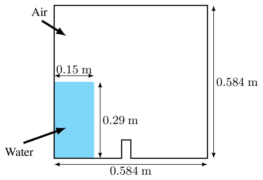
A 0.15 m×0.29 m water column initially at rest on the left-hand side of a 0.584 m×0.584 m tank otherwise filled with air is released and impacts an obstacle at the center of the tank (Fig. 1). No turbulence model is used following the original tutorial (i.e., ${\mathit{\nu }}_t^{\mathrm{f}}=\mathrm{0}$). The liquid-phase viscosity and density are specified as ${\mathit{\nu }}^{\mathrm{l}}=\mathrm{1}\times {\mathrm{10}}^{-\mathrm{6}}$ m² s⁻¹ and ρ^l=1000 kg m⁻³, while the gas-phase viscosity and density are ${\mathit{\nu }}^{\mathrm{g}}=\mathrm{1.48}\times {\mathrm{10}}^{-\mathrm{5}}$ m² s⁻¹ and ρ^g=1 kg m⁻³. The surface tension coefficient is σ=0.07.

Figure 1 Sketch of the dam-break benchmark.

The same numerical parameters are used for both the interFoam tutorial case and the present test case for a fair comparison. No-slip boundary conditions are applied on the left, right, and bottom walls, and the top boundary is exposed to the atmosphere and permits both inflow and outflow. The mesh is composed of 9072 cells with a grid size on the order of 4 cm. An implicit first-order scheme (Eulerian) is used for time integration, and second-order upwind schemes are used to discretize the convection terms. The time step is adaptive and is calculated to ensure a Courant–Friedrichs–Lewy (CFL) number that is lower than 1. This case is run sequentially.

The comparisons between sedInterFoam and interFoam at 0, 0.3, and 0.6 s are presented in Fig. 2. The time evolution of the air–water interface (defined by γ=0.5) calculated by sedInterFoam is in very good agreement with interFoam. The shape and dynamics of the liquid phase impacting the obstacle are recovered, and generation of air pockets downstream of the obstacle is reproduced. The implementation of the free-surface evolution algorithm in sedInterFoam is therefore equivalent to that in interFoam. Discrepancies only appear at 0.6 s, when the flow becomes highly chaotic and initially small differences can lead to totally different results. Considering the numerical treatment of the three-phase flow equations, this behavior can be expected.

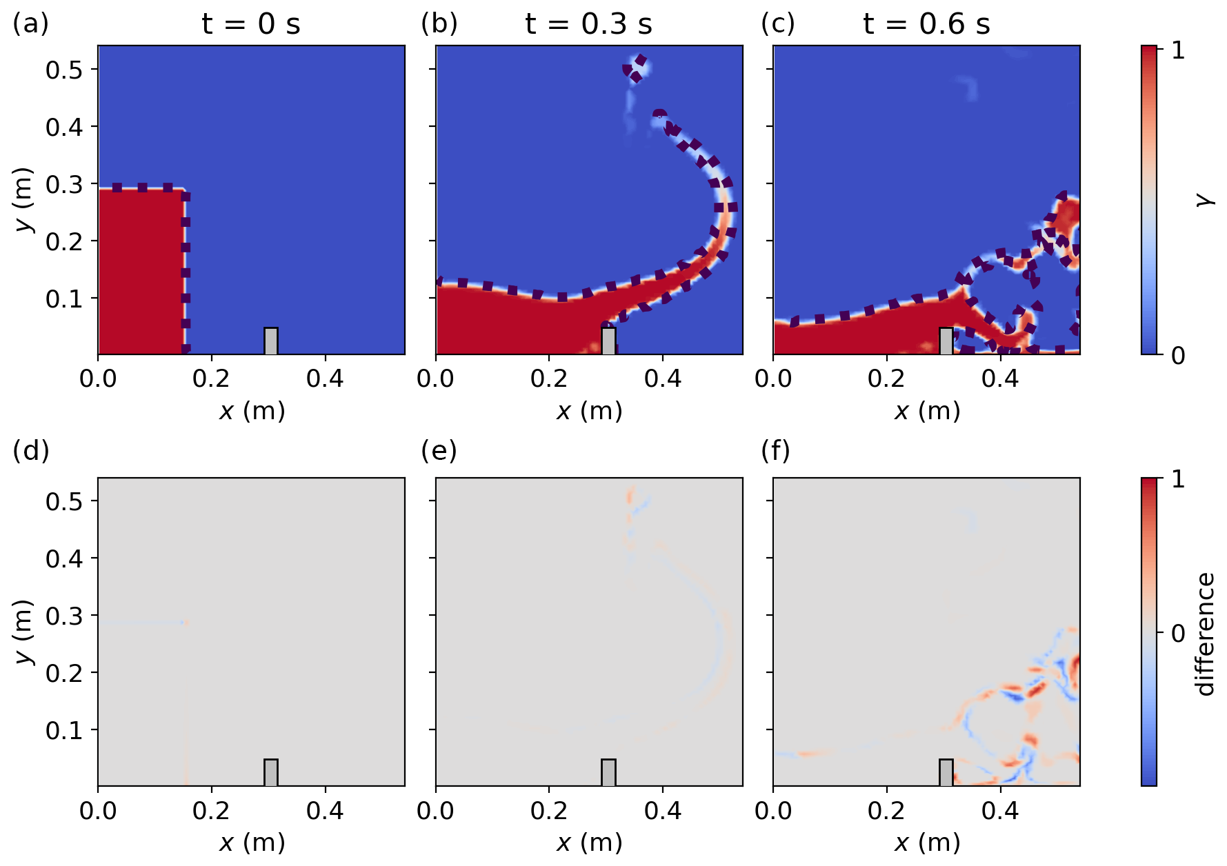
Figure 2 Comparison between the γ field from sedInterFoam represented by the color map and interFoam with the air–water interface represented by a dashed line (a–c). Differences between the γ fields from sedInterFoam and interFoam (d–f) at 0 s (a, d), 0.3 s (b, e), and 0.6 s (c, f) for the dam-break configuration.

4.2 Sedimentation

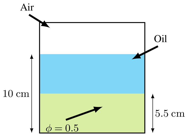
The sedimentation benchmark taken from Chauchat et al. (2017) is reproduced with sedInterFoam but with an air–water interface specified in the top portion of the domain for comparison with experimental data obtained by Pham-Van-Bang et al. (2008) and validation of the solid and liquid coupling using the pressure–velocity algorithm, momentum exchange term, and mass conservation.

The configuration consists of a suspension of monodispersed polystyrene particles of diameter d_p=290 µm and density ρ^s=1050 kg m⁻³ in Rhodorsil silicone oil with a density of ρ^l=950 kg m⁻³ and viscosity ${\mathit{\nu }}^{\mathrm{l}}=\mathrm{1.02}\times {\mathrm{10}}^{-\mathrm{5}}$ m² s⁻¹. The mixture is initially well-mixed in the bottom portion of the tank, with a particle concentration of ϕ=0.5 before sedimentation. The time evolution of the concentration is monitored in the experiment using a proton MRI device.

The numerical domain is 1D vertically decomposed into 240 cells over a depth of 12 cm. Compared with the sedFoam tutorial, an additional air layer with the same physical parameters as the dam-break benchmark presented in Sect. 4.1 is added at the top of the domain in order to be able to validate the mass conservation of the three phases throughout the simulation (Fig. 3). The time step is fixed at Δt=0.01 s. A first-order implicit time-integration scheme (Eulerian) and a second-order total variation diminish (TVD) scheme for convection terms are used. A wall boundary condition is applied at the bottom, and the pressure is fixed at the top to serve as a reference. The gradients of all the other quantities are set to zero at the top boundary. This case is run sequentially.

Figure 3 Sketch of the 1D sedimentation benchmark.

While settling, the sediment concentration profile shows two distinct interfaces. The upper interface corresponds to the transition between ϕ=0 and ϕ=0.5, while the lower interface corresponds to the transition between ϕ=0.5 and the maximum concentration in the settled bed. A comparison of the temporal locations of these two interfaces in the experiment and in the simulation is presented in Fig. 4a, while the concentration profiles at 232, 652, 1072, and 1492 s are shown in Fig. 4b. Very good agreements are observed with the measured data. For this benchmark, the performance of sedInterFoam is very similar to that of sedFoam reported in Chauchat et al. (2017). The spikes in the volume fraction for the numerical results come from numerical oscillations at the interface because of the sharp concentration gradient. This behavior has also been observed with the sedFoam solver and results from the difficulty in handling the propagation of a shock by the mass conservation equations.

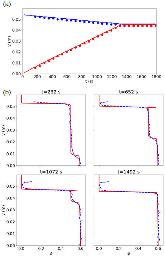
Figure 4 Temporal evolution of the upper (blue) and lower (red) interfaces in the pure sedimentation configuration (panel a, with symbols for the experimental results and the solid line for the simulation results) and concentration profiles at t=232, 652, 1072, and 1492 s (panel b, with the experimental results represented by the dashed blue line and the simulation results represented by the solid red line).

The temporal evolution of the total volume fraction difference compared with the initial values for the three phases is presented in Fig. 5. While the total volume fraction of the particles is conserved throughout the simulation, some variations are observed for the air and oil phases at the beginning. This is attributed to the time needed for the model to adapt from the initial conditions. After a few seconds, their total volume fractions evolve very slowly. Overall, the total volume fraction differences for the air and water phases remain lower than 0.5 %. To conclude, the model and its implementation allow us to reproduce the pure sedimentation, agreeing with the measured data, and the mass conservation is preserved well.

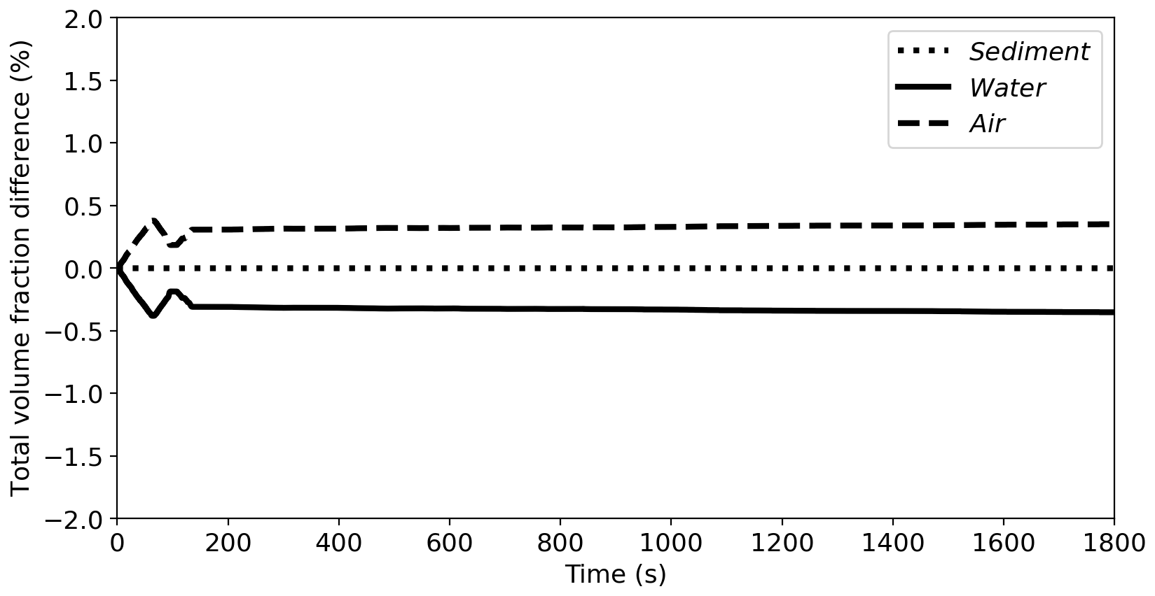
Figure 5 Time evolution of the total volume fraction difference for the solid, liquid, and gas phases in the 1D sedimentation configuration.

4.3 Sheet flow under monochromatic waves

To validate the coupling with the waves2Foam library for surface wave generation and to show sedInterFoam capabilities on unstructured grids, an experimental configuration of the sheet flow driven by monochromatic non-breaking waves from Dohmen-Janssen and Hanes (2002) is reproduced numerically with sedInterFoam. Cnoidal waves with a wave period of T=6.5 s and a wave height of H=1.55 m are generated and propagate over a bed composed of sand particles with a median diameter d_p=240 µm and a density ρ^s=2650 kg m⁻³ in a flume 3.5 m deep in the measurement section. Conductivity concentration meters buried in the sand measured the time series of the sediment concentration and allow for comparison with the model results.

The numerical configuration used for this benchmark is the same as the configuration investigated by Kim et al. (2018). In a Reynolds average field, the flow is homogeneous in the spanwise direction and a 2D configuration is established. The numerical flume is 151.56 m in length, and a sediment pit 4 m long and 0.1 m deep is located in the middle of the flume (Fig. 6). The mesh is generated with the OpenFOAM utilities blockMesh and snappyHexMesh. It is composed of around 2.85 million grid points with refined cells at the air–water and water–sediment interfaces. Details of the mesh close to the sand pit can be observed in Fig. 7. Wall boundary conditions are applied at the bottom, while the top boundary is exposed to the atmosphere, waves are generated using a 10th-order streamfunction on the left-hand side of the flume in the relaxation zone, and a sponge layer on the right-hand side of the flume allows us to absorb incoming waves and prevent reflection. The time step is adaptive to ensure a maximum CFL number lower than 0.4. A second-order backward time integrator is used, and a second-order TVD scheme is used for the convection terms. Turbulence is modeled using the two-phase k-ε model, and the kinetic theory for granular flows is used to model the shear-dependent solid-phase stresses. This case was run in parallel on 180 cores for 72 h.

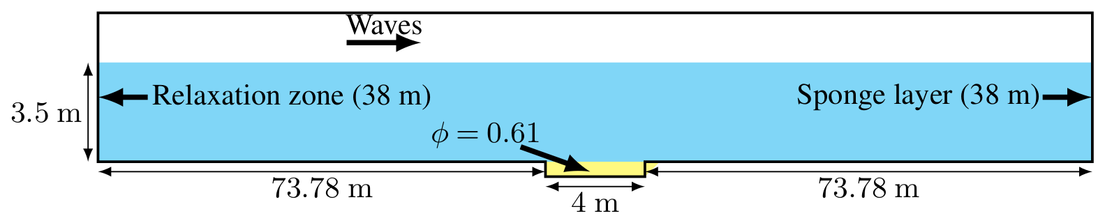
Figure 6 Sketch of the sheet flow configuration under monochromatic waves, similar to the large-wave flume experiment of Dohmen-Janssen and Hanes (2002).

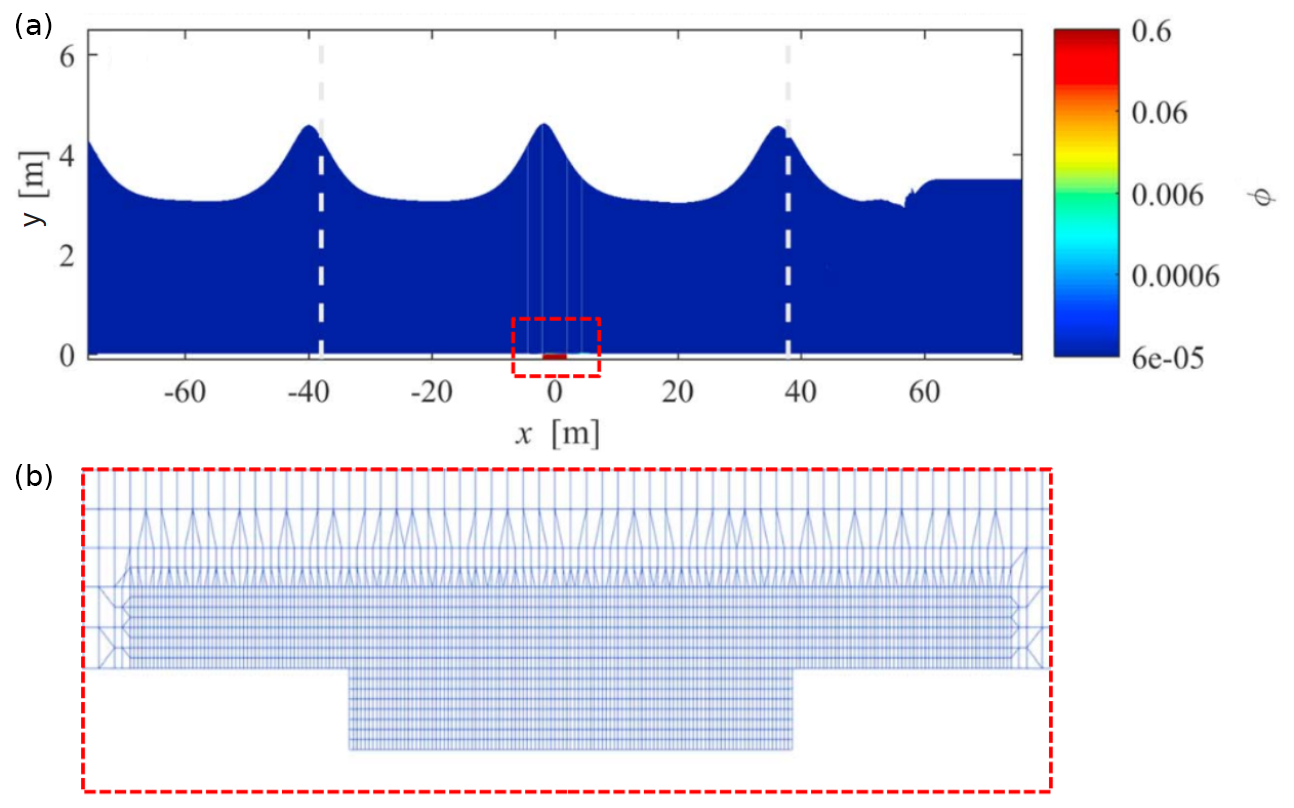
Figure 7 Snapshot of the sheet flow with a monochromatic-wave numerical configuration showing air in white, water in blue, and sediment in red (a), together with the details of the mesh (b). For visibility, the mesh is downsampled and the vertical scale is stretched by a factor of 7. The dashed lines in the top panel correspond to the relaxation zones for wave generation on the left and the sponge layer on the right.

To validate the wave generation implementation through coupling with waves2Foam and the model's capacity to predict sheet flow processes under surface waves, time series of the free stream velocity above the sediment bed and concentration profiles taken in the middle of the sediment pit at the wave crest, flow reversal, and wave trough are compared with measured data in Fig. 8. The good agreement in the time series of the free stream velocity highlights the ability of sedInterFoam to simulate nonlinear surface wave processes and validates a proper implementation of waves2Foam.

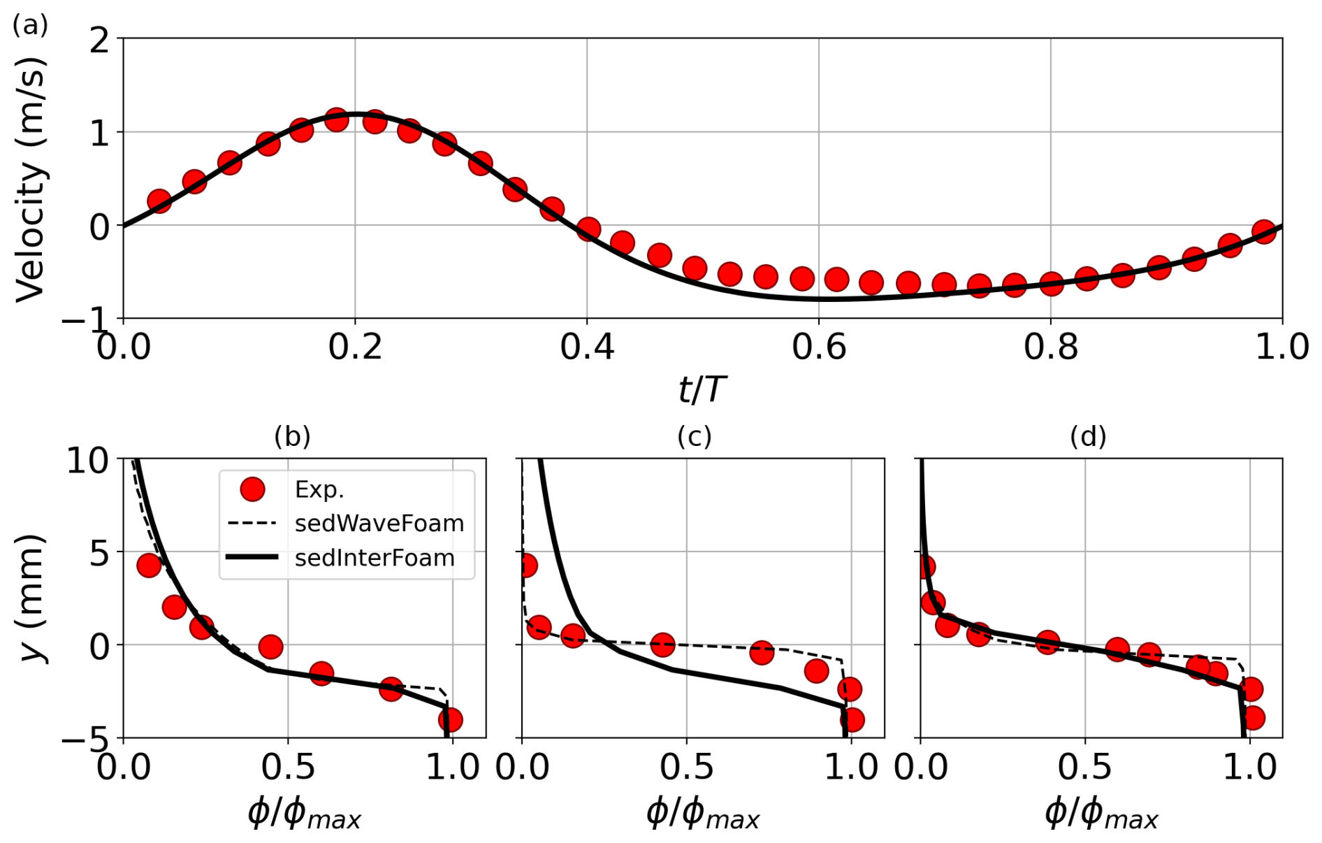
Figure 8 Time series of the free stream velocity above the sediment pit (a) and the sediment concentration profiles at the wave crest (b), flow reversal (c), and wave trough (d).

For the concentration profiles, numerical results are in good agreement with the measured data. Discrepancies can be observed at flow reversal, for which suspended sediments are slightly overpredicted. Turbulence closure parameters controlling the equilibrium between settling and upward turbulent diffusion of sediment may be responsible for the overpredicted sediment suspension. Careful tuning of the model parameters would allow more quantitative agreement between numerical and experimental results but is beyond the scope of this study. Results may also be sensitive to grid resolution and other turbulence models. The same conclusions apply for the comparison with the previous model, sedWaveFoam. The results are almost identical, except at flow reversal. Differences in the implementation of the equations and turbulence closure parameters can affect the vertical turbulent diffusion of sediment.

4.4 Plunging solitary wave

In order to demonstrate the novel capabilities of sedInterFoam for a more complex coastal application, an experimental configuration reported by Sumer et al. (2011) for a plunging solitary wave over an erodible bed is reproduced numerically. The solitary wave propagates in a flume with a 0.4 m water depth and breaks on top of a beach with a 1:14 slope composed of sand with a median diameter of d_p=180 µm. Information about the solitary wave characteristics is given in Sumer et al. (2011). In the experiment, Sumer et al. (2011) recorded the beach profile evolution after the impact of four identical solitary waves. In the simulation, successive solitary waves are generated after intervals of 20 s. This has been shown to be enough time for the free surface to become still again. This is a critical test of sedInterFoam for simulating the challenging process of beach erosion in the swash zone.

Assuming spanwise homogeneity of the Reynolds average flow, the numerical configuration is 2D. The left part of the flume is 12 m long with a constant water depth of 0.4 m. The right portion of the flume consists of a 1:14 sloping beach loaded with sediment (see Fig. 9). The sediment bed is 0.15 m deep at the toe and 0.05 m deep at the top of the beach. The mesh is composed of 1.2 million grid points. The time step is adaptive to ensure a maximum CFL number lower than 0.3. The same numerical schemes as for the sheet flow in the monochromatic-wave configuration presented in Sect. 4.3 were used. The k−ε turbulence model is used, and solid-phase stress is modeled using the μ(I) rheology. This case was run in parallel on six cores for 30 h (four successive solitary waves).

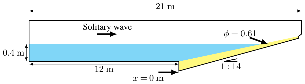
Figure 9 Sketch of the plunging solitary wave configuration, similar to the laboratory experiment reported by Sumer et al. (2011).

Snapshots of the simulation showing the impact of the first solitary wave are presented in Fig. 10. Please note that the maximum value of the color bar is larger than the maximum concentration in order to avoid saturation. At t=8.5 s (top-left panel of Fig. 10), the incoming solitary wave starts to break and erodes sediment at x=5.5 m (the origin of the x axis corresponds to the toe of the sloping beach). The morphological changes resulting from the passage of breaking waves at around x=5.6 to 5.7 m are already visible at t=11 s (top-right panel of Fig. 10), which corresponds to the end of the uprush phase. During backwash at t=13 s (bottom-left panel of Fig. 10), a hydraulic jump reported by Sumer et al. (2011) is also observed between 4.5 and 5.2 m, under which sediment accumulates. Eventually, at t=20 s (bottom-right panel of Fig. 10), the free surface returns to rest, and the accretive pattern between 4.5 and 5 m and the erosive pattern further landward become more evident.

Figure 10 Snapshots of the sediment concentration ϕ at t=8.5, 11, 13, and 20 s from the simulation of the first solitary wave impacting the sloping beach. The local coordinate x=0 m is defined at the toe of the sloping beach.

Surface elevation numerically monitored at the toe of the beach (x=0 m) and in the swash zone (x=4.63 and 5.35 m) is compared to the rigid-bed experimental data in Fig. 11. The shape of the incoming solitary wave is captured well by sedInterFoam at the different locations across the domain. At x=4.63 m (second panel of Fig. 11), a significant decrease in the water surface between 8 and 12 s is underestimated by the model. This time interval corresponds to the rundown phase when the newly formed hydraulic jump is migrating rapidly seaward, while strong shear suspends sediment close to the free surface. As a result, the differences observed in the free-surface elevation may be a consequence of interactions between sediment and water that are not present in the rigid-bed experiments.

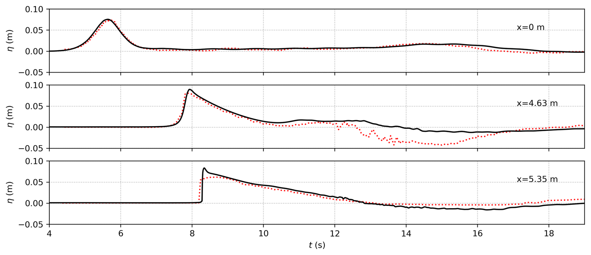
Figure 11 Free-surface elevation at x=0 m (toe of the beach), x=4.63 m, and x=5.35 m from simulations with sedInterFoam (black solid lines) compared with rigid-bed experimental data from Sumer et al. (2011) (red dotted lines).

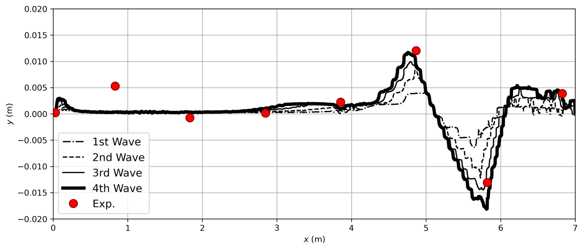
Figure 12 Morphological evolution of the sediment bed after four consecutive solitary waves from sedInterFoam simulation compared with the experimental results from Sumer et al. (2011).

To compare the predictive capabilities of sedInterFoam, the evolution of the bed profile after four solitary waves is compared to the experiments in Fig. 12. Following the laboratory experiment, each successive solitary wave is sent after the previous solitary wave impact to the flow field, and the bathymetry diminishes. The distinctive beach profile evolution features that can be observed from the measured data are accretions between 4 and 5 m corresponding to the location where a hydraulic jump is observed during backwash and erosion between 5 and 6 m, corresponding to the intermittently wet and dry areas of the beach (i.e., the upper swash). The position and amplitude of the morphological changes in the erosion and accretion zone between 3 and 7 m are predicted fairly well by sedInterFoam, with an error of less than 10 % in the region between 2 and 7 m with respect to the distance between the highest deposition and deepest scouring points. More experimental points would be required to draw conclusions about the accuracy of the model in the swash zone between 6 and 7 m. However, the model does not reproduce the accretion zone located at around 1 m that corresponds to the formation of a sandbar with an error of around 20 %. The processes involved in the generation of this morphological feature most certainly include interaction between turbulence and sand particles in suspension. Such processes would require better parameterization of RANS turbulence models or use of turbulence-resolving simulations.

Overall, the presented simulation is a proof of concept where the morphodynamics in the swash zone can be simulated numerically using sedInterFoam. This new open-source model will allow us to further investigate fine-scale hydromorphodynamic processes in order to answer the many open questions in this field.

5 Conclusions

In this paper, sedInterFoam, an extension of the two-phase flow solver sedFoam (Chauchat et al., 2017) implemented using the open-source library OpenFOAM (Jasak and Uroić, 2020), was presented. A third phase representing the air is included to model sediment transport applications driven by surface waves. The air–water interface is solved using the VOF method, similar to interFoam (Rusche, 2003; Klostermann et al., 2013) but adapted for the present miscible liquid–solid phase. Coupling with the waves2Foam library (Jacobsen et al., 2012) is implemented to generate and absorb free-surface waves. sedInterFoam includes all the previous features present in sedFoam, such as turbulence models (RANS or LES) and solid-phase stress models (kinetic theory for granular flows and μ(I) rheology).

The model has been applied successfully to a 2D dam-break configuration to benchmark the numerical results with those produced by the existing OpenFOAM solver interFoam in order to verify the implementation of the free-surface evolution algorithm. A comparison between sedInterFoam and sedFoam has been performed by simulating a 1D sedimentation configuration in order to confirm that the implementation of a third phase did not affect the mass conservation of each phase. A sheet flow configuration under monochromatic waves from Kim et al. (2018) was reproduced successfully, indicating that the implementation of waves2Foam for wave generation and absorption is appropriate. Eventually, an experimental configuration of a solitary wave plunging on a sandy beach with a slope of 1:14 (Sumer et al., 2011) was reproduced numerically to highlight the capabilities of sedInterFoam in simulating complex wave breaking, swash dynamics, and beach profile evolution. Quantitative agreement between the measured and simulated results is obtained, particularly regarding the erosion and deposition processes in the swash zone.

The development of the open-source three-phase flow model sedInterFoam provides a modeling tool for investigating coastal sediment transport applications dominated by surface waves. While relatively computationally expensive, the physics-based model sedInterFoam can be a useful tool for gaining insight into the complex physical processes associated with breaking waves, sediment transport, and morphodynamics and providing simulation data to improve empirical parameterizations in regional-scale morphodynamic models.

Appendix A: Derivation of the indicator function transport equation

In this section, the steps to derive the γ transport equation are presented. Summing the mass conservation equations for the solid, liquid, and gas phases (Eqs. 1, 2, and 3) and assuming $u_i^{\mathrm{l}}=u_i^{\mathrm{g}}=u_i^{\mathrm{f}}$ because of the non-slip boundary condition at the air–water interface allows us to write the mixture conservation equation as

$$\begin{array}{}\text{(A1)}& {\displaystyle \frac{\partial }{\partial x_i}}\left[\mathit{\varphi }{u}_i^{\mathrm{s}}+(\mathrm{1}-\mathit{\varphi })u_i^{\mathrm{f}}\right]=\mathrm{0}.\end{array}$$

Expanding Eq. (A1) and rearranging the terms gives

$$\begin{array}{}\text{(A2)}& {\displaystyle \frac{\partial }{\partial x_i}}\left[\mathit{\varphi }{u}_i^{\mathrm{f}}\right]={\displaystyle \frac{\partial }{\partial x_i}}\left[\mathit{\varphi }{u}_i^{\mathrm{s}}\right]+{\displaystyle \frac{\partial u_i^{\mathrm{f}}}{\partial x_i}}.\end{array}$$

Starting from the liquid-phase mass conservation Eq. (2), expanding it, and using the chain rule for the derivation of the products gives

$$\begin{array}{}\text{(A3)}& {\displaystyle \frac{\partial }{\partial t}}\left[\mathit{\gamma }\right(\mathrm{1}-\mathit{\varphi }\left)\right]+{\displaystyle \frac{\partial }{\partial x_i}}\left[\mathit{\gamma }(\mathrm{1}-\mathit{\varphi })u_i^{\mathrm{f}}\right]=\mathrm{0},\text{(A4)}& {\displaystyle }\Rightarrow {\displaystyle \frac{\partial \mathit{\gamma }}{\partial t}}-{\displaystyle \frac{\partial \mathit{\varphi }\mathit{\gamma }}{\partial t}}+{\displaystyle \frac{\partial }{\partial x_i}}\left[\mathit{\gamma }{u}_i^{\mathrm{f}}\right]-{\displaystyle \frac{\partial }{\partial }}\left[\mathit{\gamma }\mathit{\varphi }{u}_i^{\mathrm{f}}\right]=\mathrm{0},\text{(A5)}& {\displaystyle }\begin{array}{rl}{\displaystyle }\Rightarrow & {\displaystyle \frac{\partial \mathit{\gamma }}{\partial t}}-\mathit{\varphi }{\displaystyle \frac{\partial \mathit{\gamma }}{\partial t}}-\mathit{\gamma }{\displaystyle \frac{\partial \mathit{\varphi }}{\partial t}}+{\displaystyle \frac{\partial }{\partial x_i}}\left[\mathit{\gamma }{u}_i^{\mathrm{f}}\right]\\ {\displaystyle }& {\displaystyle }-\mathit{\varphi }{\displaystyle \frac{\partial }{\partial x_i}}\left[\mathit{\gamma }{u}_i^{\mathrm{f}}\right]-\mathit{\gamma }{u}_i^{\mathrm{f}}{\displaystyle \frac{\partial \mathit{\varphi }}{\partial x_i}}=\mathrm{0}.\end{array}\end{array}$$

Rearranging the terms of Eq. (A5) allows us to write

$$\begin{array}{}\text{(A6)}& {\displaystyle }(\mathrm{1}-\mathit{\varphi })\left[{\displaystyle \frac{\partial \mathit{\gamma }}{\partial t}}+{\displaystyle \frac{\partial }{\partial x_i}}\left[\mathit{\gamma }{u}_i^{\mathrm{f}}\right]\right]-\mathit{\gamma }\left[{\displaystyle \frac{\partial \mathit{\varphi }}{\partial t}}+u_i^{\mathrm{f}}{\displaystyle \frac{\partial \mathit{\varphi }}{\partial x_i}}\right]=\mathrm{0},\text{(A7)}& {\displaystyle }\begin{array}{rl}{\displaystyle }\Rightarrow & {\displaystyle }(\mathrm{1}-\mathit{\varphi })\left[{\displaystyle \frac{\partial \mathit{\gamma }}{\partial t}}+{\displaystyle \frac{\partial }{\partial x_i}}\left[\mathit{\gamma }{u}_i^{\mathrm{f}}\right]\right]\\ {\displaystyle }& {\displaystyle }-\mathit{\gamma }\left[{\displaystyle \frac{\partial \mathit{\varphi }}{\partial t}}+{\displaystyle \frac{\partial }{\partial x_i}}\left[\mathit{\varphi }{u}_i^{\mathrm{f}}\right]-\mathit{\varphi }{\displaystyle \frac{\partial u_i^{\mathrm{f}}}{\partial x_i}}\right]=\mathrm{0}.\end{array}\end{array}$$

Replacing the second-to-last term of Eq. (A7) with Eq. (A2) and remembering the solid-phase mass conservation Eq. (1) reads as

$$\begin{array}{}\text{(A8)}& {\displaystyle }\begin{array}{rl}{\displaystyle }(\mathrm{1}-\mathit{\varphi })& {\displaystyle }\left[{\displaystyle \frac{\partial \mathit{\gamma }}{\partial t}}+{\displaystyle \frac{\partial }{\partial x_i}}\left[\mathit{\gamma }{u}_i^{\mathrm{f}}\right]\right]\\ {\displaystyle }& {\displaystyle }-\mathit{\gamma }[\underset{\text{=0}}{\underbrace{{\displaystyle \frac{\partial \mathit{\varphi }}{\partial t}}+{\displaystyle \frac{\partial }{\partial x_i}}\left[\mathit{\varphi }{u}_i^{\mathrm{s}}\right]}}+{\displaystyle \frac{\partial u_i^{\mathrm{f}}}{\partial x_i}}-\mathit{\varphi }{\displaystyle \frac{\partial u_i^{\mathrm{f}}}{\partial x_i}}]=\mathrm{0}.\end{array}\end{array}$$

Rearranging the terms allows us to obtain the final form of the γ transport equation following

$$\begin{array}{}\text{(A9)}& {\displaystyle }\Rightarrow (\mathrm{1}-\mathit{\varphi })\left[{\displaystyle \frac{\partial \mathit{\gamma }}{\partial t}}+{\displaystyle \frac{\partial }{\partial x_i}}\left[\mathit{\gamma }{u}_i^{\mathrm{f}}\right]\right]-\mathit{\gamma }{\displaystyle \frac{\partial u_i^{\mathrm{f}}}{\partial x_i}}+\mathit{\gamma }\mathit{\varphi }{\displaystyle \frac{\partial u_i^{\mathrm{f}}}{\partial x_i}}=\mathrm{0},\text{(A10)}& {\displaystyle }\Rightarrow (\mathrm{1}-\mathit{\varphi })\left[{\displaystyle \frac{\partial \mathit{\gamma }}{\partial t}}+{\displaystyle \frac{\partial }{\partial x_i}}\left[\mathit{\gamma }{u}_i^{\mathrm{f}}\right]-\mathit{\gamma }{\displaystyle \frac{\partial u_i^{\mathrm{f}}}{\partial x_i}}\right]=\mathrm{0},\text{(A11)}& {\displaystyle }\Rightarrow {\displaystyle \frac{\partial \mathit{\gamma }}{\partial t}}+{\displaystyle \frac{\partial }{\partial x_i}}\left[\mathit{\gamma }{u}_i^{\mathrm{f}}\right]-\mathit{\gamma }{\displaystyle \frac{\partial u_i^{\mathrm{f}}}{\partial x_i}}=\mathrm{0}.\end{array}$$