The MESSy DWARF (based on MESSy v2.55.2)

The adaptation of Earth system model (ESM) codes to modern computing architectures is challenging as ESMs consist of a multitude of different components. Historically grown and developed by scientists rather than software engineers, the codes of the individual components are often interwoven, making the optimisation of the ESMs rather challenging, if not impossible. Thus, in the last few years, the codes have become increasingly modularised, and, with that, different components are now disentangled from each other. This helps porting the code section by section to modern computing architectures, e.g. to GPUs.

For more than 20 years, the modularisation has been the fundamental concept of the Modular Earth Submodel System (MESSy). It is an integrated framework providing data structures and methods to build comprehensive ESMs from individual components. Each component, e.g. a cloud microphysical scheme, dry deposition of tracer gases, or diagnostic tools, as output along satellite orbits, is coded as an individual so-called submodel. Each submodel is connected via the MESSy infrastructure with all other components, together forming a comprehensive model system. MESSy was mainly developed for research in atmospheric chemistry, and, so far, it has always been connected to a dynamical (climate or weather forecast) model, i.e. what we call a base model. The base model is a development outside the MESSy framework. Running a full dynamical model for technical tests when porting only one submodel is a tedious task and unnecessarily resource-consuming. Therefore, we developed the so-called MESSy DWARF, a simplified base model based on the MESSy infrastructure. We implemented the definition of a very simple grid, a parallelisation scheme, and a time control to replace a fully fledged base model.

The MESSy DWARF serves as a valuable tool for technical applications, such as porting individual component implementations to GPUs and performance tests or as an easy test environment for process implementations. Due to the MESSy structure, the applied components can be used in a dynamical model without any changes because the interface is exactly the same. Furthermore, the MESSy DWARF is suited for scientific purposes running simplified models (with only a selection of components), e.g. a chemical box model for the analysis of chamber experiments or a trajectory box model imitating an air parcel rising slowly into the stratosphere. Column and plume models could also easily be built based on the DWARF.

In this article, we introduce the technical setup of the MESSy DWARF and show four example applications: (1) a simple application using a component calculating orbital parameters, (2) a chemical kinetics model including photolysis frequency calculation, (3) an application of a chemical box model, and (4) some details on a GPU performance test of the chemical kinetics model.

1 Introduction

This article describes the design concept of the MESSy DWARF. The DWARF establishes a standard tool to easily create simplified setups for technical tests. This is of major concern for the process of porting such a large code base as MESSy stepwise to GPU and for performance analysis of individual submodels. Moreover, the possibility of easily developing simplified MESSy models in a unified way, e.g. box or column models, to focus on local processes without the need to consider horizontal transport was still missing within the MESSy framework.

The basic concept of the MESSy DWARF is to use MESSy data types and methods (for further details, see Sects. 2 and 3) to provide the technical framework required to run one specific process implementation (a submodel in MESSy terminology) to be able to concentrate in an efficient way on the optimisation of this specific process implementation or to “build” simplified models by combining a number of process implementations. To reach this goal, a model grid, the (distributed-memory) parallel domain decomposition, and a time control, which are usually provided by the dynamical models, need to be provided by MESSy. Before the DWARF development, MESSy already provided all data types and methods required to

• initialise the model variables by reading input data and transforming (remapping) it to the actual model grid;

• produce output of not only instantaneous values but also of namelist-driven standard diagnostic output as minima, maxima, averages, etc.;

• control the time-stepping and checkpointing;

• perform a tendency analysis for prognostic variables.

But for real applications, MESSy was always connected to a dynamical model. The idea to fully utilise the capacity of the MESSy framework to build simplified models, especially for testing and also for simpler scientific applications, was triggered by the publication of Müller et al. (2019). Earth system models (ESMs), especially those including explicit atmospheric chemistry process descriptions, are very expensive in terms of required computing time and memory. As these models have been developed over a long time, they are not straightforwardly efficiently applicable or even portable to new computing architectures. This problem is faced by most models of this kind around the world. Therefore, a strategy on how “to evolve weather and climate prediction models to next-generation computing technologies” (Müller et al., 2019) was developed within the ESCAPE (Energy-efficient Scalable Algorithms for Weather Prediction at Exascale) funded by HORIZON2020 (https://research-and-innovation.ec.europa.eu/funding/funding-opportunities/funding-programmes-and-open-calls/horizon-2020, last access: 11 February 2025). The first point of this strategy is to “(i) identify domain-specific key algorithmic motifs in weather prediction and climate models (which we term Weather & Climate Dwarfs)” (Müller et al., 2019, “Introduction” section). “The dwarfs thus represent domain-specific mini-applications (Messer et al., 2018) which include direct input from the domain scientist together with documentation” (Müller et al., 2019, Sect. 2.1). With the publication of Müller et al. (2019), the idea of restructuring comprehensive, established source codes to separate them into smaller pieces related to specifically simulated processes, or, in short, the idea of formally modularising the source codes, became widely acknowledged in the community after already having been proposed in 2005 (Jöckel et al., 2005).

Combining the basic design concepts of the Modular Earth Submodel System (MESSy, Jöckel et al., 2005), i.e. that each component is already coded as an individual submodel, with the “dwarf strategy” developed and published by the ESCAPE project (Müller et al., 2019), resulted in the development of the MESSy DWARF.

While the ESCAPE Weather & Climate Dwarfs are seven specific dwarfs for seven process implementations, the MESSy DWARF adds a new base model to the MESSy framework, enabling running each MESSy submodel (currently, more than 90 are available, and the number is growing) in simplified setups. Each individual ESCAPE dwarf solves the problems by setting up its own minimal driver (grid, parallelisation etc.), while the MESSy DWARF is a generic base model with which all process descriptions, available as MESSy submodels, can be applied. The ESCAPE dwarfs have the advantage that the overhead is minimal, thus providing the perfect setup to optimise this specific process.

In contrast, the MESSy DWARF requires some additional overhead to the individually tackled submodel always using the above listed MESSy functionalities. While the larger overhead could be considered a downside for performance optimisation, it is an upside that the MESSy DWARF establishes a standard model, which can be used to drive all submodels, avoiding the need to develop individual drivers for each specific submodel. Furthermore, since the submodel interfaces are the same for all base models according to the MESSy concept, a submodel developed or optimised in a DWARF configuration can be directly used in a fully fledged base model without any changes. Additionally, it is possible to run and test combinations of submodels with the DWARF. This is not only helpful for technical optimisations (see Sect. 4.4), but also to open up the DWARF for scientific use, e.g. for simplified models such as chemical box models (see Sect. 4.3).

Starting with a short introduction into the basic MESSy concept (Sect. 2), the following section provides an overview of the technical realisation of the MESSy DWARF (Sect. 3). Section 4 contains several examples of DWARF applications to illustrate its usability. Finally, the article is concluded with a short summary and a list of some future development plans (Sect. 5).

2 The MESSy infrastructure and submodel concept

The Modular Earth Submodel System (MESSy, Jöckel et al., 2005) is an integrated software framework which was initially built to facilitate the implementation of atmospheric chemistry processes into existing models of atmospheric dynamics (Jöckel et al., 2010; Kerkweg and Jöckel, 2012). Its basic idea is that each process and diagnostics can be coded as an individual submodel. Such a submodel consists of two parts: the submodel core layer (SMCL) contains the implementation of the process coded in its basic entity (e.g. kinetics is represented by a box and convection by a column process), while the submodel's interface layer (SMIL) connects to the MESSy infrastructure components on the (base-model-dependent) base-model interface layer (BMIL), which in turn is connected to the base-model layer (BML), i.e. the base model (see Fig. 1). This four-layer software architecture allows for the implementation of the SMCL to be completely independent of the base model, for instance, its local variable dimensions, order of ranks, and parallel decomposition.

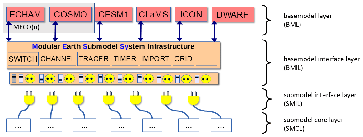
Figure 1 Sketch of the four-layer code structure of MESSy. The image illustrates how the different base models and the base-model-independent core layer of the individual submodels are interconnected via the two interface layers. The base-model interface layer (BMIL) organises the correct workflow and data exchange between the regular submodels, the cores of which are connected by the submodel interface layer (SMIL) to the BMIL.

Jöckel et al. (2010)Jöckel et al. (2005)Jöckel et al. (2005)Kerkweg et al. (2018)Kerkweg and Jöckel (2015)(Dietmüller et al., 2016)Jöckel et al. (2005)Eichinger and Jöckel (2014)Jöckel et al. (2010)Jöckel et al. (2008)Sander et al. (2014)Sander et al. (2019)Dietmüller et al. (2016)Hofmann et al. (2016)

Table 1 List of MESSy submodels including a short description and citation (if possible).

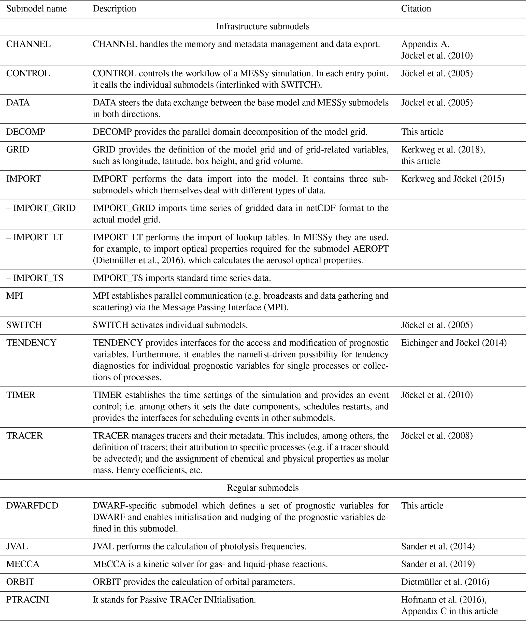
MESSy distinguishes between regular submodels and infrastructure submodels. While the regular submodels are realisations of individual processes (e.g. the kinetic solver for the gas-phase chemistry, dry deposition and convection) or diagnostics, the MESSy infrastructure submodels establish the overall machinery required to orchestrate the individual submodels (data exchange, control flow, checkpointing, data import and export, etc.). Thus, the infrastructure submodels establish the framework to execute the regular submodels. The MESSy infrastructure submodels comprise – among others – submodels for

• memory management and output control (submodel CHANNEL, Appendix A¹, Jöckel et al., 2010);

• import of data (submodel IMPORT, Kerkweg and Jöckel, 2015);

• time and event control (submodel TIMER, Jöckel et al., 2010);

• data exchange between the base model and MESSy submodels (submodel DATA, Jöckel et al., 2005);

• flow control, i.e. activation of submodels (submodel SWITCH), and calling of the submodels during simulation (CONTROL, Jöckel et al., 2005);

• tracer data and tracer metadata handling (submodel TRACER, Jöckel et al., 2008);

• tendency diagnostic (submodel TENDENCY, Eichinger and Jöckel, 2014).

Table 1 lists the MESSy submodels mentioned in this publication, including a very short description and respective references.

If MESSy is connected to a dynamical model, the dynamical model defines the grid, provides the parallel domain decomposition information, including methods for data transpositions (e.g. based on the Message Passing Interface, MPI) and the set of prognostic variables and external data, such as the land–sea mask and surface elevation. This information is picked up by the MESSy infrastructure submodels and translated into MESSy data types for harmonised usage by all MESSy submodels.

3 The technical realisation of the MESSy DWARF

So far, MESSy has always been connected to dynamical models, e.g. the global climate model ECHAM5 (Roeckner et al., 2006; Jöckel et al., 2010) or the regional weather and climate model COSMO (Rockel et al., 2008; Kerkweg and Jöckel, 2012). However, for simplified scientific applications or for technical tests (such as source code optimisation), a dynamical model is not always required or even counterproductive due to unnecessary overhead, e.g. for performance analysis of a single MESSy submodel.

As for the MESSy DWARF, the base model is basically “empty”; all functionalities and data usually provided by the base model and made accessible via the MESSy infrastructure to the submodels need to be replaced by either additional infrastructure functionalities (e.g. the definition of a grid) or import of external data. The chemical kinetics submodel MECCA (Model Efficiently Calculating the Chemistry of the Atmosphere, Sander et al., 2019) is used as an example to demonstrate the dependence of a process submodel on entities usually provided by the base model and to illustrate the concept of the DWARF.

To meaningfully set up the DWARF, with MECCA being the only regular MESSy submodel used, three main aspects need to be considered:

• 1.

  The provision of input data required by MECCA. These are the following:

  • i.

    The temperature and the specific humidity. Temperature and specific humidity are prognostic variables. Dynamical base models provide the set of prognostic variables as determined by their dynamical core. In MESSy, these are made accessible to the MESSy submodels via the infrastructure submodel TENDENCY (see Sect. 3.1.1). As the DWARF does not contain a dynamical core, the regular MESSy submodel DWARFDCD (DWARF's Dynamical Core Dummy) simply provides a set of prognostic variables (see Sect. 3.1.1).

  • ii.

    The photolysis frequencies. The photolysis frequencies are usually calculated by the MESSy submodel JVAL (Sander et al., 2014). Given a setup where MECCA is the only used regular submodel, J values need to be provided as external data. External data are imported via the MESSy infrastructure submodel IMPORT (see Sect. 3.1.2).

  • iii.

    The pressure at box mid-points. The pressure is provided by the base model itself and referenced by the MESSy infrastructure submodel DATA, or, if the base model does not provide a pressure field, it is calculated in DATA. Thus, in the case of the MESSy DWARF as well, it is calculated or referenced by DATA (see Sect. 3.1.3). In the case of a reference, it will relate to external data provided by IMPORT_GRID (see Sect. 3.1.2).

  • iv.

    The tracers (chemical active trace species). The tracers are created by MESSy submodels, i.e. in the example, by MECCA. The tracer metadata and memory management is provided by MESSy infrastructure submodel TRACER and the data are accessed and changed via the infrastructure submodel TENDENCY (same as the other prognostic variables). Thus, tracers are handled in exactly the same way for the DWARF as for legacy base models.

  • v.

    The longitude and latitude fields for debug output. Last but not least, for debug output, the longitude and latitude fields are required by MECCA. These are always provided by the MESSy infrastructure submodel GRID_DEF (see in Sect. 3.2) independently of the base model.

• 2.

  The handling of the output data provided by MECCA. MECCA solves the kinetic equations of the gas-phase chemistry and calculates the change in reactive chemical species over a time increment; thus, the output of MECCA consists of the tendencies of the reactive trace gases. These tendencies, i.e. the rate of change for the current time step inferred by kinetics, are fed back via the TENDENCY infrastructure model.

• 3.

  The grid on which the simulation should be performed. A full dynamical model naturally provides a grid on which the primitive equations and the model physics are solved. For the DWARF, a simple grid is defined by the infrastructure submodel GRID_DEF (see in Sect. 3.2). Additionally, the parallel domain decomposition of the grid and the parallel communication patterns need to be established (Sect. 3.3) if working in (distributed-memory) parallel environments.

The following subsections provide more details on how the features listed above are implemented in the MESSy DWARF.

3.1 Data supply

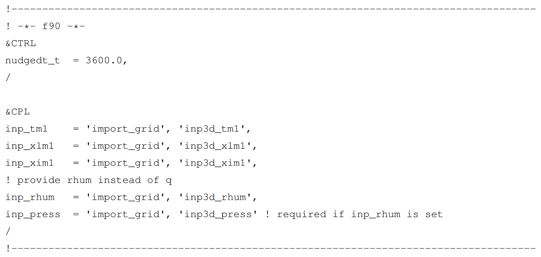
Figure 2 Example namelist file, dwarfdcd.nml, for the MESSy submodel DWARFDCD. According to the &CPL namelist, all prognostic variables provided by DWARFDCD except q are initialised from external data read by IMPORT_GRID. q is initialised from an imported relative humidity field. For this calculation, additionally, the pressure field is required, which is also provided by IMPORT_GRID. The only time-varying, i.e. nudged, prognostic variable is the temperature, as a nudging coefficient is defined only for this in the &CTRL namelist.

In the usual MESSy model setup using a legacy model as the base model, the MESSy submodels have access to two types of external data:

• data provided by the base model and

• data imported by the MESSy submodel IMPORT.

The base-model data themselves separate into (i) initial and boundary data (including nudging data) and (ii) base model variables.

• i.

  Initial data are used to initialise the model and therefore are only required at the very first model time step. In contrast to this, boundary data need to be updated regularly, for example, after discrete time intervals during the model simulation.

• ii.

  Base-model variables are calculated by the base model. The most important variables are the prognostic variables, which are the variables used to solve the primitive equations. The set of prognostic variables can therefore differ between base models. Non-prognostic variables are often called diagnostic variables.

If MESSy is run in connection with a legacy base model, the base-model-specific variables are made available to the MESSy submodels by the translation of those (in the BMIL) into so-called MESSy channel objects. The technical implementation of this translation in the BMIL depends on the base model. In EMAC, for instance, the translation is based on pointer association² of channel objects to the internal data structures of the ECHAM5 base model. In COSMO/MESSy, the COSMO source code has been modified to allocate memory of the COSMO variables directly in the form of channel objects via the corresponding CHANNEL methods. Prognostic variables, specifically, are translated (i.e. made accessible) via the MESSy submodel TENDENCY (Eichinger and Jöckel, 2014). Diagnostic variables required by several MESSy submodels but not present in the respective base model are calculated in the (base-model-specific part of the) MESSy submodel DATA. One example might be the 3-dimensional geopotential height field, which is available in ECHAM5 but not in COSMO and therefore is declared and calculated in the COSMO-specific part of DATA.

The DWARF, however, is a generic (basically empty) base model without the functionality of a legacy base model. Thus, first, a set of prognostic variables needs to be defined. This is implemented within the submodel DWARFDCD (see Sect. 3.1.1). Second, all other variables in the DWARF become initial or boundary data and are imported by the MESSy submodel IMPORT.

Which set of prognostic variables is defined by the new MESSy submodel DWARFDCD and how they are modified is described next (Sect. 3.1.1). The functionality of the IMPORT infrastructure submodel is explained in Sect. 3.1.2. The last subsection (Sect. 3.1.3) describes which variables are calculated additionally by the MESSy submodel DATA.

3.1.1 Definition and modification of prognostic variable

The MESSy infrastructure submodel TENDENCY (Eichinger and Jöckel, 2014) allows for detailed analyses of individual tendencies³ of prognostic variables. Each process using a prognostic variable as input, or changing it, must access and/or modify it via methods (i.e. calling of subroutines) of the infrastructure submodel TENDENCY. In this way, it can be ensured that the operator-splitting concept is always followed (meaning implemented in a numerically correct way) and that all tendencies can be budgeted by TENDENCY if desired.

This implies that the MESSy submodels are expecting specific prognostic variables to be accessible and modifiable via TENDENCY. Therefore, for the MESSy DWARF, the new submodel DWARFDCD defines a set of the prognostic variables. Currently, the following prognostic variables are provided by DWARFDCD:

• the air temperature, t, in kelvin;

• the horizontal wind velocities, u and v, in m s⁻¹;

• the water vapour, q, in kg kg⁻¹;

• the liquid water content, x_l, in kg kg⁻¹;

• the ice water content, x_i, in kg kg⁻¹.

Due to the setup of the DWARF (i.e. without a dynamical core), the prognostic variables are only changed if a MESSy submodel adds a tendency to the respective variable. However, it might be desirable to initialise and change the content of the prognostic variables. Consequently, DWARFDCD provides an initialisation and a nudging option. Using the &CTRL namelist of the DWARFDCD namelist file (see Fig. 2), a relaxation time can be specified for each of the prognostic variables independently. The variable nudgedt_Y, with $Y=t,u,v,q,x_{\mathrm{l}},x_{\mathrm{i}}$, respectively, provides this relaxation time (in seconds) with which the respective variable is forced to follow the imported data that are accessed via the corresponding &CPL namelist entries (inp_Y). The tendency (tend_Y) added to the prognostic variable Y is then calculated as follows:

$$\begin{array}{}\text{(1)}& \mathtt{\text{tend\_Y}}=(\mathtt{\text{inp\_Y}}-\mathtt{\text{start\_Y}})/\mathtt{\text{nudgedt\_Y}},\end{array}$$

with start_Y being the current value of variable Y.

If only the initialisation, without nudging, of a prognostic variable is required, the setting of the inp_ parameters in the &CPL namelist is sufficient. A nudging coefficient must not be defined as the definition of the nudging coefficients triggers the nudging.

Note, a prognostic variable stays zero if no input data are provided and no process adds a tendency to it. This is technically possible as not all simplified DWARF setups require all prognostic variables.

As the DWARF will be used for measurement campaign analyses, a special case has been introduced for the initialisation and nudging of the water vapour mixing ratio. This is rendered useful as measurements often provide only the relative humidity. Therefore, the option was implemented to use the relative humidity (in percentages) as input for the forcing of the water vapour, q (in kg kg⁻¹), instead of prescribing the water vapour mixing ratio directly. This option is activated by providing inp_rhum instead of inp_q. Additionally, the conversion of relative humidity to specific humidity requires the pressure as input; thus, inp_press needs to be provided in the &CPL namelist.

3.1.2 Initial and boundary data

One important part of each model simulation is the provision of initial and boundary data. The MESSy infrastructure submodel IMPORT provides the standard interface for data import at the beginning of and during the model simulation. See the IMPORT user manual (available in the supplement of Kerkweg and Jöckel, 2015, or in the MESSy code distribution) for technical details and the usage of the IMPORT submodel, including a detailed description of the meaning of namelist parameters. Two sub-submodels of IMPORT (compare Table 1 and Kerkweg and Jöckel, 2015) are used for replacing base-model functionalities:

• IMPORT_GRID. The MESSy infrastructure submodel IMPORT_GRID imports 2- or 3-dimensional gridded data at the beginning of and during a simulation. Which data are imported and when is determined by namelists. The import process includes (i) reading in the requested data, (ii) distributing it according to the parallel domain decomposition, and (iii) remapping it onto the actual model grid used. The order of these steps depends on the base model used. For the DWARF and its limited-area grid (see Sect. 3.2), each parallel MPI task reads and interpolates the data for its part of the grid. The DWARF uses the SCRIP (A Spherical Coordinate Remapping and Interpolation Package) algorithm in IMPORT_GRID (Jones, 1999) for the remapping.

  Gridded data can be read once at the beginning of the simulation or in discrete time intervals during the simulation if a time series of gridded data is available. The triggers for reading and the sequences of time steps to be selected from the files are defined by a Fortran namelist as the user interface.

• IMPORT_TS. IMPORT_TS provides an interface for reading standardised time series data, i.e. data available for a specific period in time and with a specific number of parameters, from files in ASCII or netCDF format.

  In full 3-dimensional simulations, this is, for example, used to read the vertical equatorial zonal wind profile for quasi-biannual oscillation (QBO) nudging (Jöckel et al., 2016). In the case of the DWARF, IMPORT_TS is especially helpful for box-model simulations, i.e. for reading in measurement data to constrain the DWARF to the experiment conditions. Section 4.3 provides an example for this.

3.1.3 DATA provision

The MESSy infrastructure submodel DATA serves as a translator, providing the base-model data to the MESSy submodels in a harmonised way. DATA performs different operations to simplify the access to the base-model data for the submodels:

1. Variables available from different base models describing the same content might be named differently. In this case, DATA defines a channel object reference (see Appendix A) to harmonise the channel and object name with which the individual submodels access this variable.

2. Variables which are not directly available from the base model but are derivable from other variables are calculated by DATA. For these, a channel object is defined (i.e. the respective memory is allocated), and the variable is calculated during the time loop.

The first category is not available in the MESSy DWARF as, in the DWARF setup, there is no data-providing base model; i.e. the DWARF is completely driven by imported data. The second category is available for the DWARF.

Figure 3 Example namelist file, data.nml, for the MESSy submodel DATA.

Variables, which are usually provided by the dynamical model, are required by some process submodels. If these can be calculated from the basic model setup and the prognostic variables, they are calculated within DATA for the DWARF. These variables are

• the Coriolis parameter (s⁻¹),

• the vorticity (s⁻¹),

• the density of dry air (kg m⁻³).

Even more importantly, the 3-dimensional pressure fields defined at the box centres or the vertical interfaces are required by many calculations in the MESSy submodels. These can either be prescribed by imported data (in this case, the imported data need to be coupled to DATA via the &CPL namelist of DATA; see Fig. 3) or are allocated and calculated in DATA itself following the US Standard Atmosphere, 1976 (U.S. Government Printing Office, 1976), using the height fields as determined in GRID (see Sect. 3.2).

3.2 GRID_DEFinition

For the MESSy DWARF the grid is defined in the MESSy infrastructure submodel GRID_DEF. For the start, we decided to use a very simple grid as, for technical tests, only the number of grid boxes or the overall size of the grid matters. The basic grid layout is similar to the one used in the regional weather prediction and climate model COSMO (Doms and Baldauf, 2021; Rockel et al., 2008) but much more simplified as the grid defined for the DWARF in GRID_DEF does not allow for any rotation of the geographical grid and does not include halo longitudes and latitudes.

Figure 4 Illustration of the horizontal (a) and vertical (b) grid definition.

Figure 5 Example namelist file grid.nml for the MESSy sub-submodel GRID_DEF.

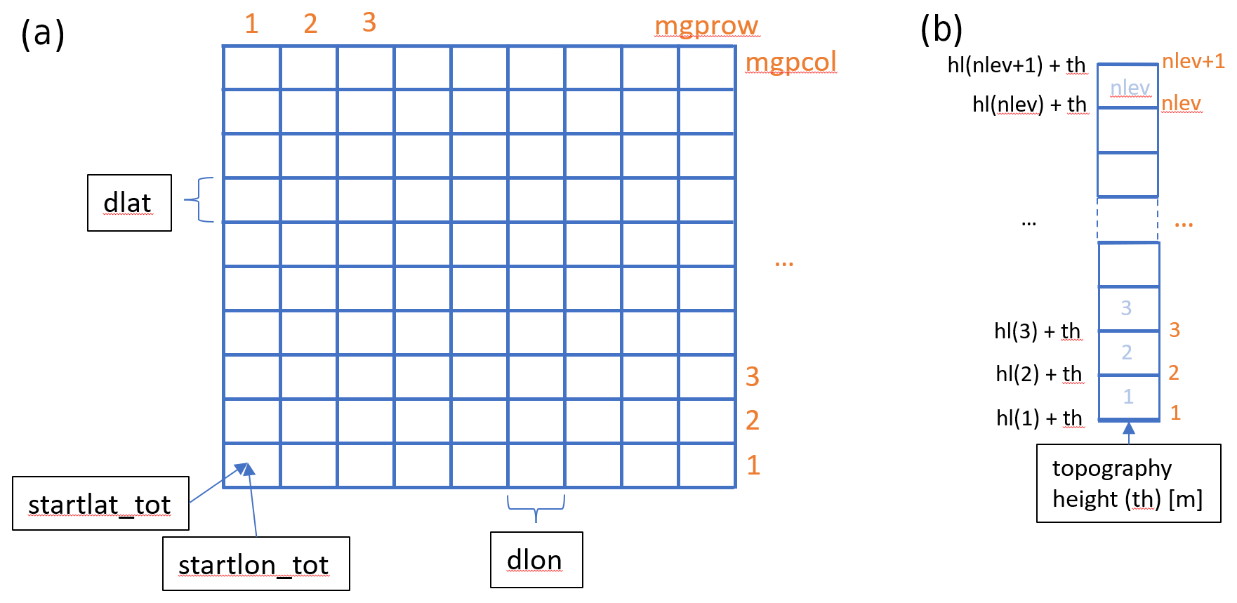
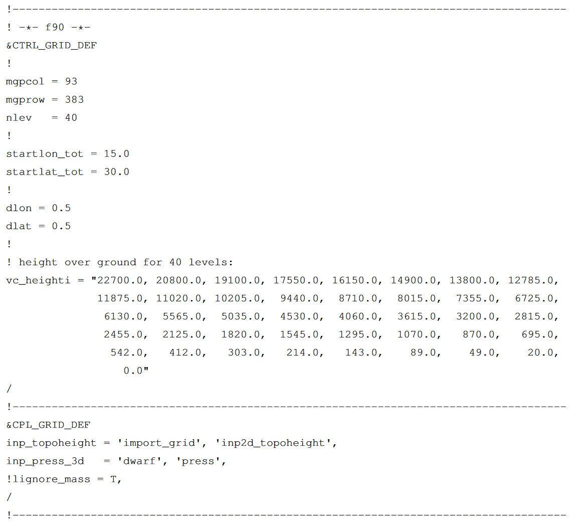
The horizontal grid is defined as a rectangle spanning a limited area (Fig. 4a), which is defined by the lower-left corner (the geographical coordinates of the grid-box centre point of the lower-left grid corner have to be provided in the GRID_DEF namelist as startlon_tot, in ° E, and startlat_tot, in ° N), the number of grid boxes in longitude and latitude directions (mgprow and mgpcol), and the grid spacing (dlon / dlat in ° E/° N, respectively). Figure 5 displays an example of the namelist file of the GRID submodel grid.nml. The above listed namelist parameters are part of the &CTRL_GRID_DEF namelist.

The vertical grid (Fig. 4b) is dimensioned by the number of vertical boxes (nlev). Their vertical extent is defined via the namelist parameter vc_heighti (formula symbol vc), which provides the heights in metres above topography (H_topo in metres) of the interface levels of the vertical grid boxes. The 3-dimensional fields containing the altitude above ground ($H^{I_{\mathrm{gnd}}}$) and the altitude above mean sea level ($H^{I_{\mathrm{msl}}}$) at the vertical interface (I) of the grid are calculated from this input as follows:

$$\begin{array}{}\text{(2)}& \begin{array}{rl}{\displaystyle }{H}^{I_{\mathrm{gnd}}}(i,j,k)& {\displaystyle }=\mathrm{vc}\left(k\right),\\ {\displaystyle }{H}^{I_{\mathrm{msl}}}(i,j,k)& {\displaystyle }=\mathrm{vc}\left(k\right)+H_{\mathrm{topo}}(i,j),\end{array}\end{array}$$

with i, j, and k being the longitudinal, latitudinal, and vertical index, respectively. The height at the box mid-levels is calculated by

$$\begin{array}{}\text{(3)}& \begin{array}{rl}{\displaystyle }{H}_{\mathrm{gnd}}(i,j,k)=& {\displaystyle }\mathrm{0.5}\times \left(H_{\mathrm{gnd}}^I\right(i,j,k+\mathrm{1})+H_{\mathrm{gnd}}^I(i,j,k\left)\right),\\ {\displaystyle }{H}_{\mathrm{msl}}(i,j,k)=& {\displaystyle }\mathrm{0.5}\times \left(H_{\mathrm{msl}}^I\right(i,j,k+\mathrm{1})+H_{\mathrm{msl}}^I(i,j,k\left)\right).\end{array}\end{array}$$

The second namelist of the GRID namelist file (Fig. 5), i.e. &CPL_GRID_DEF, defines the coupling, i.e. the input required from other MESSy submodels. In the example case, the topography is read by the MESSy submodel IMPORT_GRID, and the coupled object is named inp_topoheight. Additionally, the calculation of the air mass in the grid box and the dry air mass in the grid box require the pressure. In Fig. 5, the pressure is not pre-described but is calculated by the MESSy submodel DATA according to the US Standard Atmosphere (1976).

Last but not least, for a very reduced setup, when even the water vapour content is not known, the calculation of the grid mass can be skipped by setting the logical switch lignore_mass to true.

3.3 DECOMPosition and parallel communication (MPI)

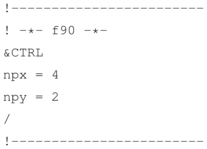
The MESSy infrastructure submodel DECOMP organises the parallel decomposition of the MESSy DWARF. The parallelisation is a classical horizontal domain decomposition along the longitudes and latitudes. The example namelist in Fig. 6 shows a decomposition along the longitudinal range into four segments and along the latitudinal range into two segments, requiring, overall, $\mathrm{4}\times \mathrm{2}=\mathrm{8}$ MPI tasks. The number of grid boxes is divided by the number of segments in each direction. If it cannot be divided without a remainder, the number of grid boxes is increased by 1 for as many tasks as correspond to the remainder. In our example, the latitude range covers 93 grid boxes, which are distributed among two segments. In this case, the tasks of the first segment get 46 grid boxes in the latitudinal direction, while the tasks in the second segment get 47 grid boxes. The same happens for the longitudinal range: $\mathrm{393}/\mathrm{4}=\mathrm{98.25}$. Thus, the tasks in the first three segments get 98 grid boxes, while the tasks in the fourth segment get 99 grid boxes. Thus, task 0 gets 98×46 grid boxes, while task 7 gets 99×47 grid boxes.

Figure 6 Example namelist file, decomp.nml, of the MESSy submodel DECOMP.

Internally, DECOMP saves the start indices of the respective local domains and determines the start longitude and latitude (startlon/startlat) of each local domain.

The parallel communication is established by the MESSy submodel MPI. It uses the Message Passing Interface (MPI) to perform the communication between the different parallel tasks. The individual broadcast, gather, and scatter routines are based on the respective implementation of the COSMO model.

3.4 Limitations of the DWARF approach

As the DWARF provides a very simplistic replacement for a fully fledged dynamical model, there are limitations to the applicability of the DWARF:

• The MESSy DWARF in its basic configuration (i.e. if only the infrastructure submodels and DWARFDCD are active) does not provide any dynamical, physical, or chemical processes; thus, if no regular MESSy submodel is switched on to provide any tendencies, prognostic variables (including tracers) will be constant in time. If they are not initialised, the prognostic variables (including tracers) will be zero. Furthermore, as long as no regular MESSy submodel contributes a transport process, the DWARF just consists of a number of independent (unconnected) boxes, which are organised on a 3-dimensional geographical grid.

• The regular MESSy submodel DWARFDCD is required to create the prognostic variables, which are accessed by the regular MESSy submodels via TENDENCY. Each of the prognostic variables needs to be initialised if it should have a meaningful value. Nudging needs to be switched on if a prognostic variable should change over time. All of these are namelist settings, and it is the obligation of the user to ensure a meaningful setup. Otherwise, prognostic variables that are zero could lead to errors.

• The currently applied simple grid is defined without halo cells; i.e. calculations, which require data of the horizontally neighbouring cells, will fail at the border of the local grid cell. As a consequence, these fields show incorrect values at the edge cells of the local domain, and the results are dependent on the chosen parallel domain decomposition. However, almost all MESSy submodels operate only on one horizontal grid cell or within a vertical column of grid cells; thus, for engineering tests, this limitation can be accepted. If the knowledge of neighbouring cells is necessary for a scientific application, the MPI communication needs to be implemented to exchange the values of the halo cells.

• The user has to take care that all the data required as input to a submodel are available from either imported data or other MESSy submodels. Missing data, however, in contrast to the first two points, will lead to an error during runtime telling the user that data are missing.

4 Example applications

This article describes the design concept of the MESSy DWARF. The major driving force for developing the DWARF was, on the one hand, the need to establish a standard tool to easily create simplified setups for technical tests. This is of major concern for the process of porting such a large code base as MESSy stepwise to GPU and for performance analysis of individual submodels. On the other hand, the possibility of easily developing simplified MESSy models in a unified way, e.g. box or column models, to focus on local processes without the need to consider horizontal transport was still missing within the MESSy framework.

Table 2 Process submodels used in example simulations.

Table 3 Basic setup of example simulations.

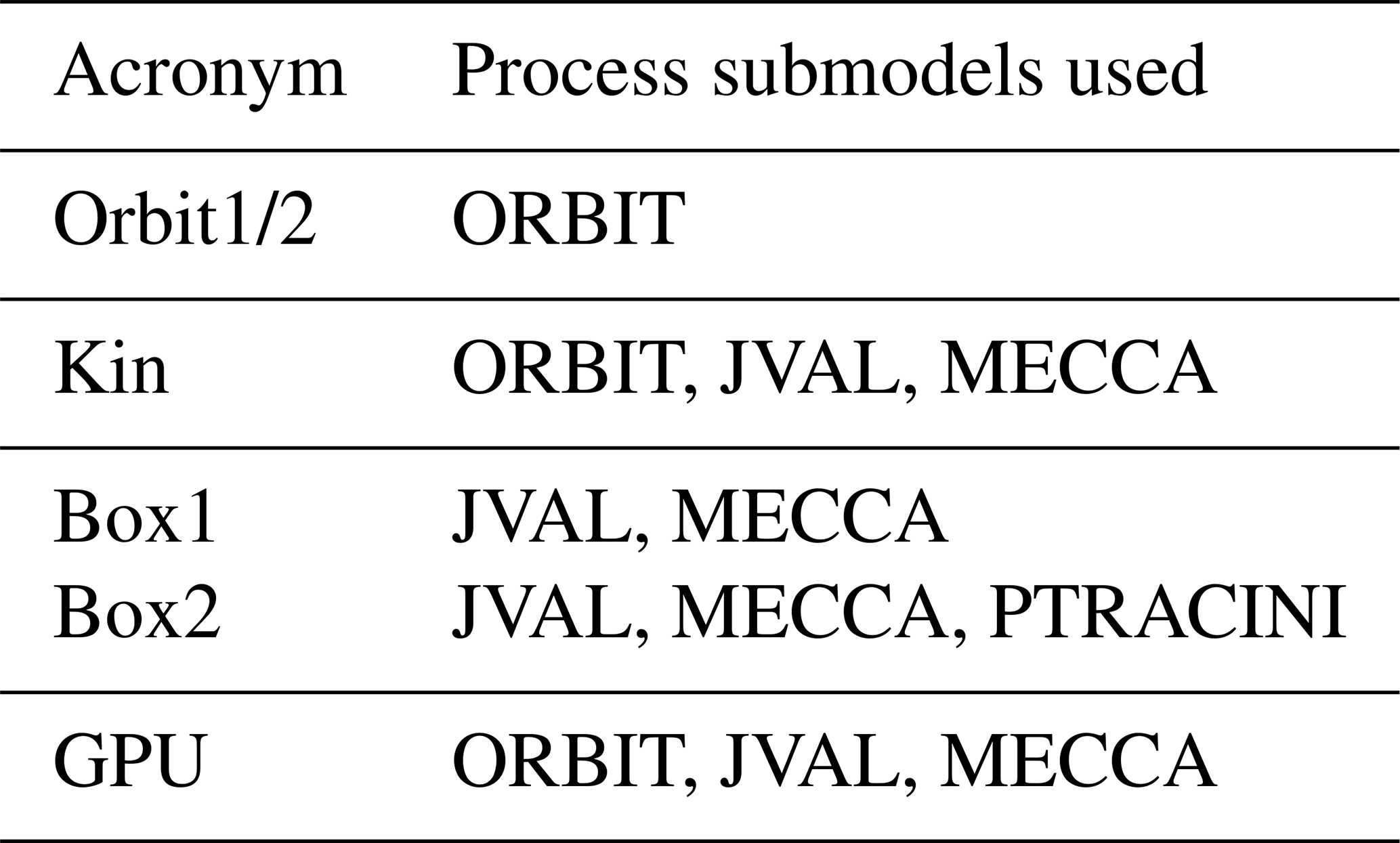
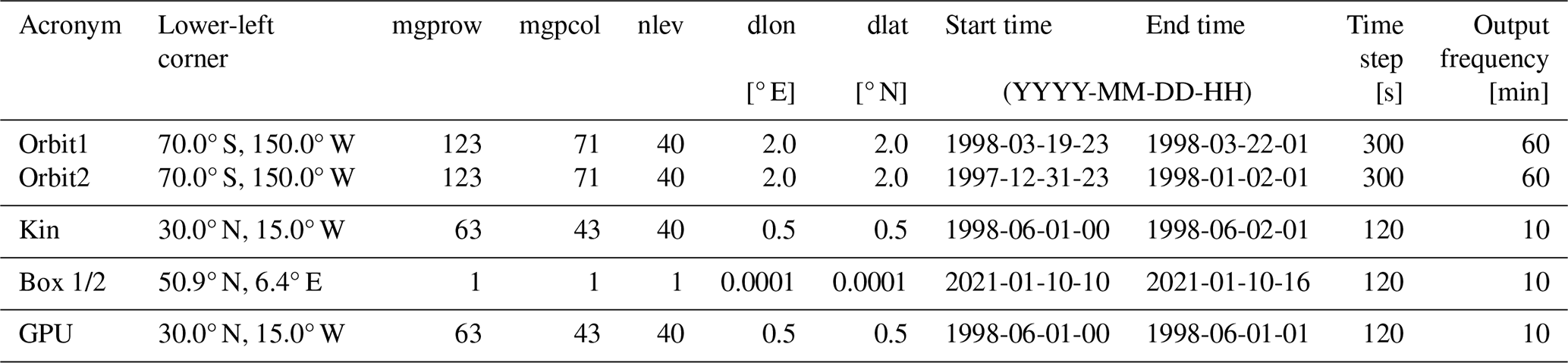
In the following, four examples for the applicability of the MESSy DWARF are presented. At the beginning, a very simple model calculating orbital variations (Sect. 4.1) is shown. A simplified 3-dimensional chemical model (Sect. 4.2) and a chemical box model (Sect. 4.3) are presented next. The last example demonstrates how a simplified 3-dimensional chemical model can be used for performance analysis in the framework of porting the chemical kinetics model to GPU (Sect. 4.4). Table 2 lists the regular submodels used for the respective examples, while Table 3 provides an overview of the respective model configurations.

4.1 Orbital variations

As the first, very simple example, the submodel ORBIT (Dietmüller et al., 2016) calculating orbital parameters is used. The only input ORBIT requires are the time and the geographical location. These are provided in the same way for all base models, including the MESSy DWARF, by the infrastructure submodel TIMER and GRID_DEF, respectively.

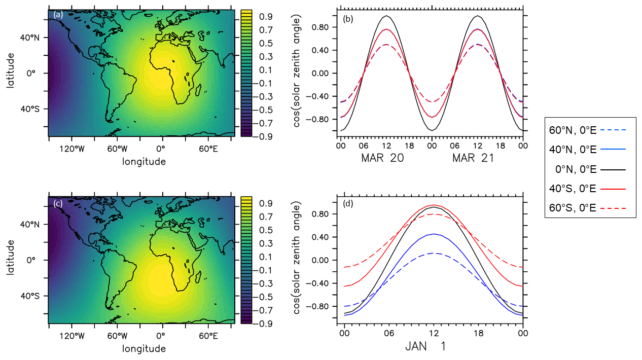
Figure 7 Cosine of the solar zenith angle calculated by the submodel ORBIT. Panels (a) and (c) show area plots over the entire model domain for 20 March 1998, 12:00 UTC (a), and for 1 January 1998, 12:00 UTC (c). Panels (b) and (d) show the diurnal cycles of the cosine of the solar zenith angle: 60° S, 40° S, 0° N, 40° N, and 60° N and 0° E for 20–21 March 1998 (b) and 1 January 1998 (d), respectively.

For this example, a simulation has been run for 20–21 March 1998 (Orbit1 in Tables 2 and 3) and 1 January 1998 (Orbit2). Figure 7 shows some of the results.

The diurnal cycle of the cosine of the solar zenith angle exhibits the largest amplitude at the Equator, and the amplitude decreases with the distance to the Equator (Fig. 7b, d). On the equinox on 20–21 March (Fig. 7b), the cosine of the solar zenith angle for 60 and 40° S equals exactly those at 60 and 40° N, respectively. However, this is only true for the equinox, while differences in the cosine of the solar zenith angle are already visible before and after the equinox. In addition, in January (Fig. 7d), the shift in the solar zenith angle according to the season for the regions nearer to the poles is apparent.

While the right panels give an impression of the modulation of the solar zenith angle from a local point of view, the left panels of Fig. 7 give a spatial impression. They present area plots of the cosine of the solar zenith angle in the model domain at 12:00 UTC. As expected, the maximum for 20 March is exactly at the Equator, while the maximum for January is shifted towards the South Pole.

4.2 The chemical kinetics model

The second example (Kin in Tables 2 and 3) is a simple 3-dimensional setup for atmospheric gas-phase chemical kinetics. The only submodels used are (see Table 2)

• the chemical kinetics submodel MECCA (Sander et al., 2005, 2019), solving the ordinary differential equation system for gas-phase chemistry, where the chemical mechanism is the same as the basic mechanism used by Jöckel et al. (2016);

• the submodel JVAL (Sander et al., 2014), calculating the photolysis frequencies required within MECCA;

• the submodel ORBIT (Dietmüller et al., 2016), providing the orbital parameters required by JVAL.

As no transport processes are included in this model setup, in fact, independent simulations in mgprow × mgpcol × nlev $=\mathrm{63}\times \mathrm{43}\times \mathrm{40}=\mathrm{108}\mathrm{360}$ grid boxes (compare Table 3) are performed. The boxes differ in their horizontal and vertical position according to the defined grid (from 30 to 51.5° N and 15° W to 16.5° E). Differences in the simulated chemistry between the individual grid boxes are due to either the initialisation of the chemical species or the prescribed external data.

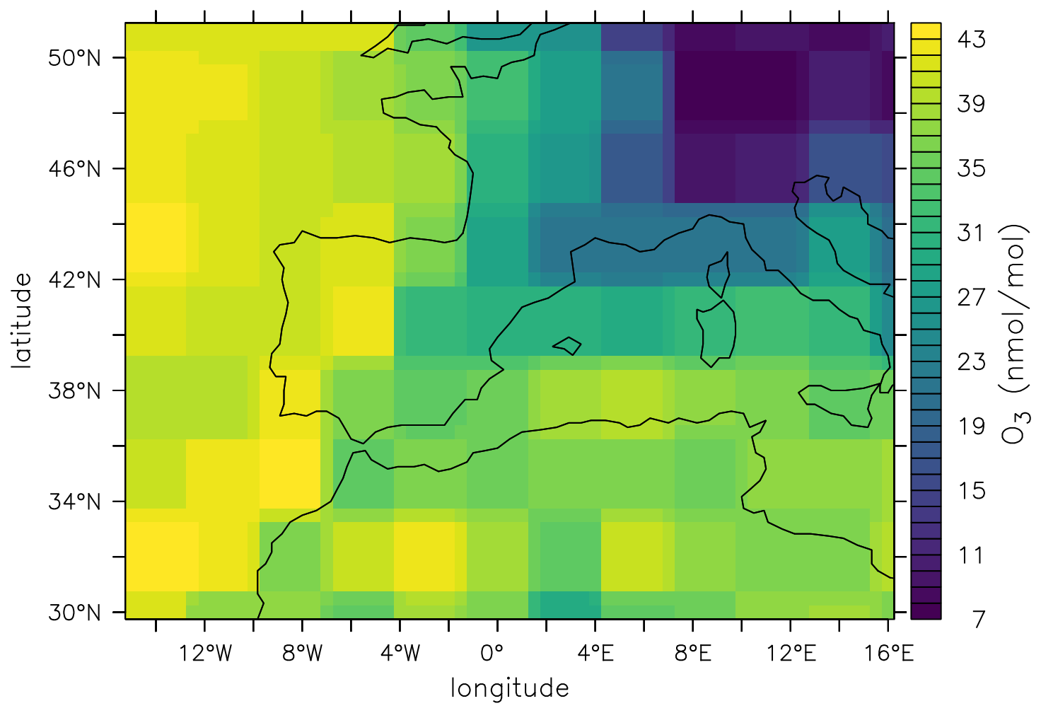
Figure 8 Ozone mixing ratio (nmol mol⁻¹) in the lowest model layer 10 min after model start (i.e. 1 January 1998, 00:10:00 UTC).

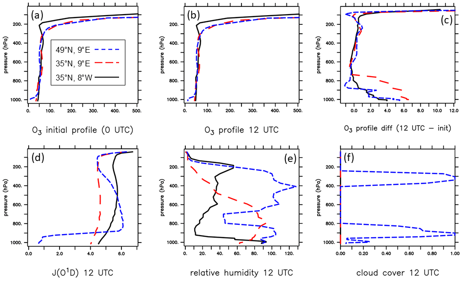
Figure 9 Ozone profiles at three geo-locations are presented: 49° N, 9° E (blue); 35° N, 9° E, (red); and 35° N, 8° W (black). The upper row displays ozone profiles (nmol mol⁻¹) at model start (1 January 1998, 00:00 UTC) (a) and at 12:00 UTC (b) and the difference between these profiles (c). The lower row depicts profiles at 12:00 UTC of the photolysis frequency of O¹D (in 10⁵ s⁻¹) (d), the relative humidity (in percentages) (e), and the cloud cover (as a fraction between 0 and 1) (f).

The inputs required by ORBIT and MECCA are discussed in Sect. 4.1 and the introduction of Sect. 3, respectively. The input fields required by JVAL are the following:

1. Firstly, the temperature, liquid water content, and ice water content are required. These are accessed via TENDENCY and are, in the MESSy DWARF, created by the submodel DWARFDCD. In DWARFDCD, they have been initialised by data imported with IMPORT_GRID. No nudging is applied. Thus, these three variables are constant over time.

2. Another required field is the ozone tracer. It is defined and modified by the submodel MECCA. Thus, it is provided in the same way in DWARF as in fully fledged base models.

3. The third requirement are the cosine of the zenith angle and the distance between the Sun and the Earth. These are provided by the MESSy submodel ORBIT.

4. Next, the ozone column above the model top and solar cycle data are required. These are made available from external data via IMPORT_GRID for all base models.

5. The pressure at box mid-points and vertical interfaces are another required input field. These are, in this DWARF setup, calculated in the infrastructure submodel DATA from the height grid defined in the infrastructure submodel GRID_DEF.

6. Finally, this includes relative humidity, land–sea fraction, cloud cover, and albedo. All four variables are usually provided by a dynamical base model; in this example, these are provided as external data, i.e. read by IMPORT_GRID.

For the initialisation of the tracers, a restart file from a former T42 EMAC simulation is used. Figure 8 displays the initial surface mixing ratio of ozone. The chessboard pattern results from the remapping of the coarse T42 (approx. 2.8° × 2.8°) resolution to the 0.5° × 0.5° grid of the DWARF.

As the reaction rates in MECCA depend on temperature, pressure, and humidity, the initialisation of these fields influences the simulated kinetics directly. Note that, in this setup, these temperature, pressure, and humidity fields are only initialised. For the sake of simplicity, they are kept constant in time. Furthermore, the calculation of the photolysis frequencies (submodel JVAL) influences the chemistry and depends itself on solar activity, orbital parameters, pressure, ozone, cloud cover, relative humidity, albedo, and surface type (land or sea).

To illustrate the spatial variation in these parameters, Fig. 9 displays vertical profiles at three different locations: 49° N, 9° E (blue); 35° N, 9° E (red); and 35° N, −8° E (black). These locations have been chosen with regard to the surface ozone (compare Fig. 8), for low (blue), medium (red), and high (black) surface ozone, respectively.

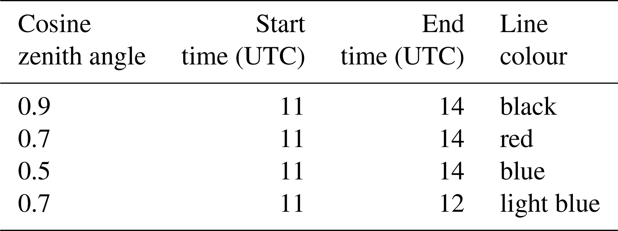
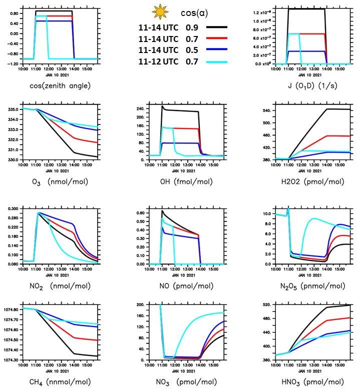
Table 4 Prescribed cosine of the solar zenith angle of the kinetic box-model study (Box1), the hours at which the sun is “switched on” and “switched off”, and the respective line colour in Fig. 10.

The upper row of Fig. 9 depicts the ozone profiles shortly after model start (left, annotated as initial) and at 12:00 UTC (middle) and the difference between these profiles (right). Ozone is the lowest in the lowest model layer, while it is some orders of magnitude higher in the stratosphere (above approx. 250 hPa). However, the difference between the vertical profiles (right panel) between the initial condition and the 12:00 UTC vertical profile exhibits different time evolutions of the profiles in each box. The bottom row of Fig. 9 displays the respective vertical profiles of the photolysis frequency of O¹D (${\mathrm{O}}_{\mathrm{3}}+h\mathit{\nu }\to {\mathrm{O}}^{\mathrm{1}}\mathrm{D}+{\mathrm{O}}_{\mathrm{2}}$, left), the relative humidity (mid), and the cloud cover (right). While the black and the red profiles are cloud-free, the blue profile exhibits two distinct cloud layers in which the 100 % relative humidity level is exceeded and supersaturation persists. Below the lower-level cloud, the photolysis frequency is much lower than for the two profiles without clouds. Above the cloud, the photolysis frequency is slightly enhanced (compared to the other two profiles), which is caused by the reflection of sunlight on top of the underlying cloud. While the red and the blue profiles are above land, the black profile is above the ocean. However, when comparing the red with the black profile, the red profile exhibits a much higher relative humidity, except for the lowest model layer. In the pressure range approximately between 980 and 500 hPa, the red profile contains much more water vapour. This is reflected in the photolysis frequencies, which are much lower for the red profile.

As atmospheric chemistry is a non-linear process, none of the shown aspects alone can explain the vertical profile of a specific chemical species as here, for example, ozone. However, using a chemical box model provides an efficient tool to test dependencies on individual parameters. How such a box model can be built with the DWARF and how it can be used is explained in the next subsection.

Figure 10 Time evolution of different parameters and chemical species in a chemical box-model simulation. Here, the cosine of the solar zenith angle (upper-left panel) is the input parameter varied (see also Table 4).

4.3 The chemical box model

In contrast to the model setup described in the subsection above, this subsection deals with a single box model, i.e. mgprow, mgpcol, and nlev are all 1, the bottom and the top height of this box are defined as vc_heighti = 15.0,5.0, i.e. the centre of the box is 10 m above the surface. The geographical location of the box is Jülich, Germany (50.9° N, 6.4° E). In the first example, only the submodels MECCA and JVAL are used. All required parameters are prescribed as time series data via IMPORT_TS. The initialisation of the chemical species, if required, is taken from the same restart file as in the previous example. As photolysis frequencies depend on the light intensity, the MESSy submodel JVAL requires information about the ozone column above the simulated chemical box. This is no problem for a 3-dimensional dynamical model (additional information about the upper-atmosphere ozone content is always required as input to JVAL); however, if only one single box should be simulated, this profile information is missing. To enable the usage of JVAL also for single box-model experiments, JVAL has been expanded by the option to use an artificial profile as vertical column information. Appendix B provides further information about this expansion of JVAL.

The following two examples are shown to demonstrate how sensitivity studies could be easily performed with such a box model.

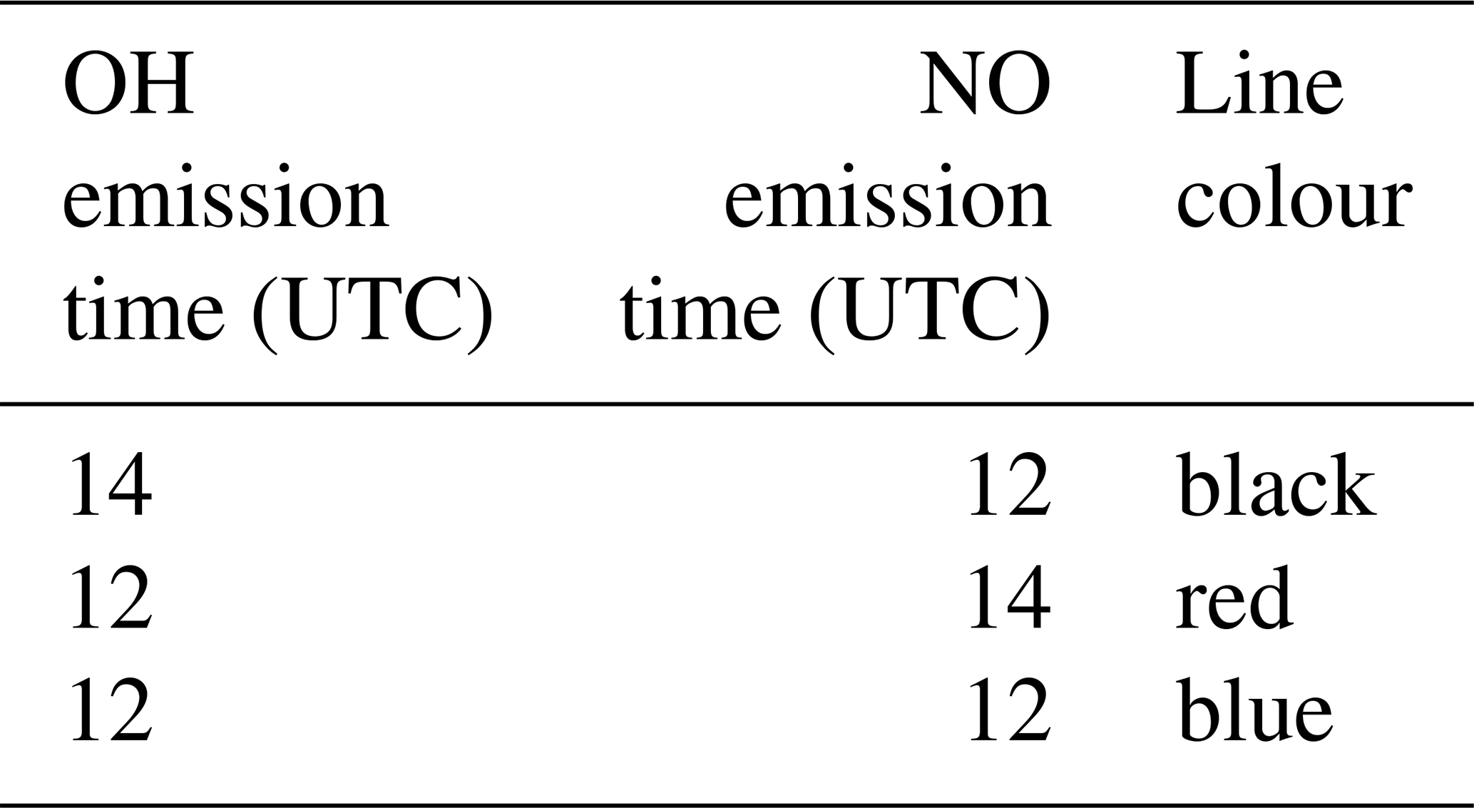
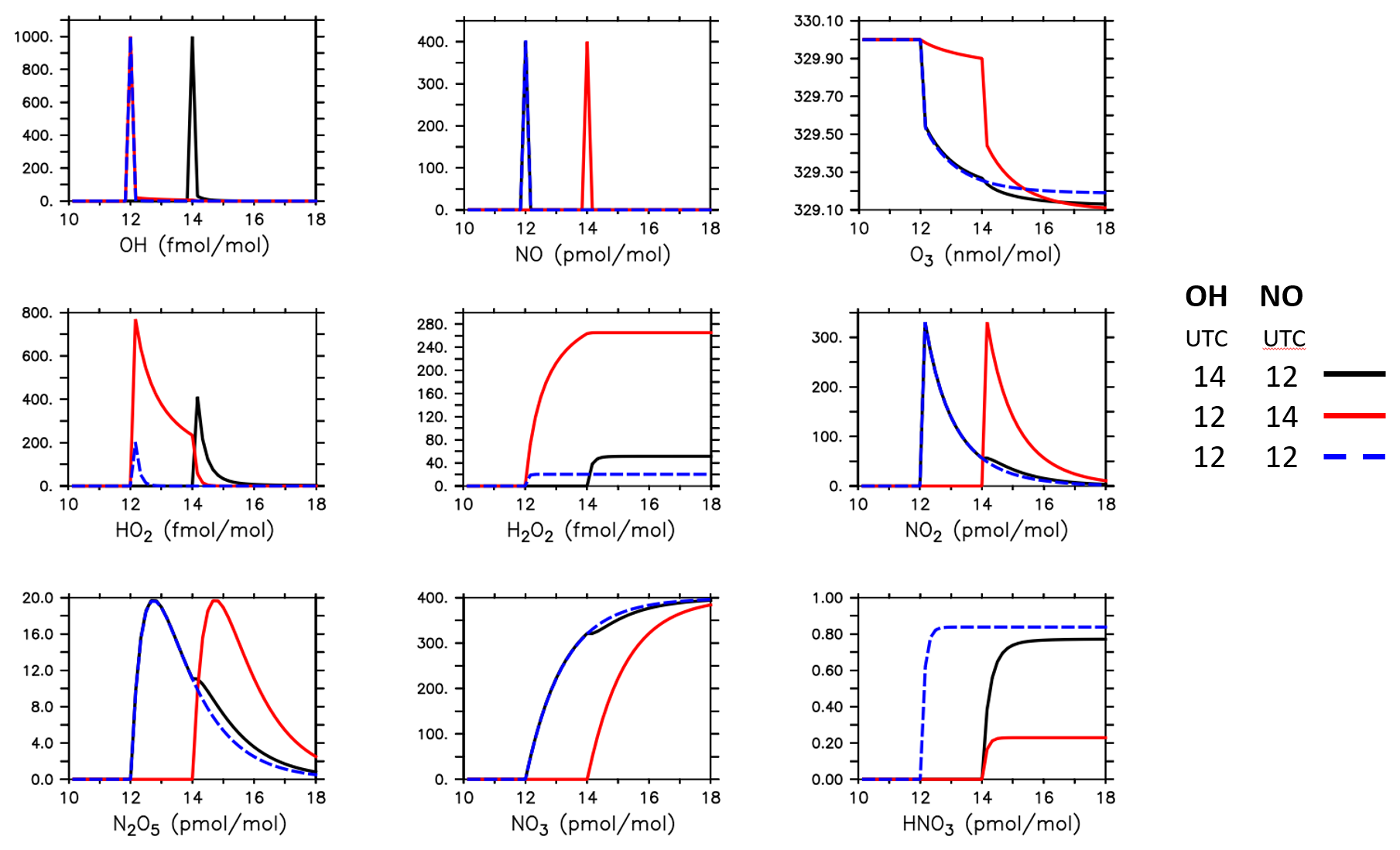
Table 5 Emission times of OH and NO in the three simulations of the idealised kinetic box-model study (Box2) and the respective line colour in Fig. 11.

4.3.1 Sensitivity to solar radiation

Four simulations (Box1 in Tables 2 and 3) have been performed, varying only one input parameter: the cosine of the solar zenith angle. Tables 3 and 4 provide an overview of the different simulations. The simulations were started at midnight in darkness. The sun was “switched on” at 11:00 UTC and “switched off” again at 14:00 UTC in three of the simulations, while in the simulation depicted in light blue, darkness prevails already from 12:00 UTC on.

Exemplary for all, the photolysis frequency of the reaction J (O¹D): ${\mathrm{O}}_{\mathrm{3}}+h\mathit{\nu }\to \mathrm{O}{(}^{\mathrm{1}}\mathrm{D})+{\mathrm{O}}_{\mathrm{2}}$ is shown in Fig. 10. Naturally, the photolysis frequency depends on the solar zenith angle: the higher the sun above the horizon, the larger the photolysis frequency. This artificially triggered onset and offset of photochemistry is mirrored in the time evolution of all nine chemical species depicted in the remaining nine panels. The higher the photolysis frequencies are, the faster

• ozone decreases (mainly due to ${\mathrm{O}}_{\mathrm{3}}+h\mathit{\nu }\to \mathrm{O}{(}^{\mathrm{1}}\mathrm{D})+{\mathrm{O}}_{\mathrm{2}}$),

• OH increases (mainly driven by $\mathrm{O}{(}^{\mathrm{1}}\mathrm{D})+{\mathrm{H}}_{\mathrm{2}}\mathrm{O}\to \mathrm{2}\mathrm{OH}$),

• H₂O₂ increases (mainly due to $\mathrm{2}{\mathrm{HO}}_{\mathrm{2}}\to {\mathrm{H}}_{\mathrm{2}}{\mathrm{O}}_{\mathrm{2}}+{\mathrm{O}}_{\mathrm{2}}$),

• methane decreases (mainly driven by ${\mathrm{CH}}_{\mathrm{4}}+\mathrm{OH}\to {\mathrm{CH}}_{\mathrm{3}}+{\mathrm{H}}_{\mathrm{2}}\mathrm{O}$), and

• HNO₃ increases (mainly due to ${\mathrm{NO}}_{\mathrm{2}}+\mathrm{OH}\to {\mathrm{HNO}}_{\mathrm{3}}$).

The other species show a much more complicated time evolution, visualising the non-linear interactions in atmospheric chemistry.

4.3.2 Idealised experiment

The second example (Box2) presents a very idealised setup. In a simulation running from 10:00 to 18:00 UTC, all chemical species except for ozone are initialised with a value of zero. Ozone is initialised with a mixing ratio of 330 nmol mol⁻¹. Photochemistry is switched off as the cosine of the solar zenith angle is set to −1. The simulation setups trigger OH and NO emissions at 12:00 UTC and/or 14:00 UTC. Table 5 provides an overview of the setups. The results (Fig. 11) show a clear dependence of the production and destruction of the individual species on the emission times of NO and OH:

• Ozone is more efficiently destroyed by NO. If OH and NO are emitted at the same time, competing reactions lead to overall less ozone destruction (= larger ozone mixing ratio at the end of the simulation).

• If only OH is emitted first, HO₂ forms most efficiently because nitrogen oxides do not compete with the HO₂ building reactions ${\mathrm{O}}_{\mathrm{3}}+\mathrm{OH}\to {\mathrm{HO}}_{\mathrm{2}}+{\mathrm{O}}_{\mathrm{2}}$. Consequently, H₂O₂ is also built most efficiently if OH is emitted first.

• Nitrogen oxides can only be built if NO is emitted. NO₂ is produced most efficiently, along with NO₃ and consequently N₂O₅ buildup, if NO is emitted into the system.

• HNO₃ can only be built (${\mathrm{NO}}_{\mathrm{2}}+\mathrm{OH}\to {\mathrm{HNO}}_{\mathrm{3}}$) if hydrogen and nitrogen are both added to the system. It forms most efficiently if OH and NO are emitted simultaneously. By far less HNO₃ forms if OH is added first as, in this case, most hydrogen ends up in H₂O₂, which cannot be converted to HNO₃ without photochemistry.

Figure 11 Time evolution of chemical species in a chemical box-model simulation. Only ozone (O₃) was initialised. OH and NO were emitted at 12:00 and 14:00 UTC in different order (see the main text and Table 5 for the respective line colours).

4.4 Performance tests: GPU port of chemical kinetics

This last example illustrates the usefulness of the DWARF for performance analysis. Analysing a specific submodel is much easier if the model configuration can be significantly simplified compared to complex base models. A smaller code base allows for a simpler and faster usage of performance analysis tools as the time required to create the runtime profiles is significantly reduced.

Table 6 Runtime comparison between CPU and GPU for two chemical mechanisms (MIM and MOM) on one JUWELS BOOSTER node.

Here, the same simple 3-dimensional setup, as described in Sect. 4.2, was used to analyse and compare the runtime of the MECCA submodel operated either entirely on CPUs or executing the chemical kinetic calculations on GPUs. The MEDINA tool (Alvanos and Christoudias, 2017; Christoudias et al., 2021) was used to create the CUDA code of the kinetics integration.

Additionally, MECCA ran with two different reaction mechanisms: firstly, the standard mechanism (MIM, Mainz Isoprene Mechanism), taking into account 159 species and 360 reactions. The more complex mechanism based on MOM (Mainz Organic Mechanism, Sander et al., 2019) has 729 species with 2193 reactions. Obviously, due to the larger matrix to be solved, it is expected that the more complex mechanism shows an even greater speedup on GPU. Profiling was done with the NVIDIA Nsight Systems tool (https://developer.nvidia.com/nsight-systems, last access: 25 March 2024) on the JUWELS BOOSTER high-performance computing (HPC) system (Jülich Supercomputing Centre, 2021) by adding special markers to the DWARF code to enable the tracing of the code parts which are of interest here. On this machine, one computing node equipped with two AMD EPYC 7402 processors and four NVIDIA A100 40GB was used. For the CPU run, the GPUs were disabled. The runtime⁴ of the integration phase for these variants are displayed in Table 6. Additionally, Fig. 12 visualises the tracing displayed by the NVIDIA Nsight Systems tool for two subsequent time-loop passes during the integration. Here, mecca_physc contains the call to the kinetic solver. Obviously, running the kinetic solver on GPUs speeds up not only the integration of the kinetics per se (Table 6, right), but also the overall runtime (Table 6, left) is reduced by a substantial amount, i.e. a factor 2.36 and 4.21 for MIM and MOM, respectively. The more complex chemistry shows a much higher speedup as the larger vector of chemical species results in more calculations, which can utilise the capability of the GPUs better.

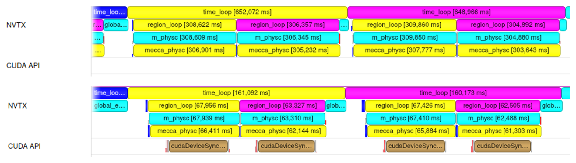
Figure 12 Example of an NVIDIA Tools Extension Library (NVTX) tracing with the NVIDIA Nsight Systems tool for the DWARF integration of the MIM chemical mechanism. Visualised are two subsequent time steps, including the call of the kinetics integration (upper panel: CPU only, lower panel:kinetics integration on GPUs).

5 Summary and outlook

The new MESSy generic base model DWARF is presented here. It was developed to provide the basis for a unified testing of individual MESSy submodels for model performance analysis and improvement and, last but not least, as a basis for setting up simplified models (e.g. box and column models) in a standardised way using all functionalities provided by the MESSy framework.

The examples presented in Sect. 4 of this article illustrate that the DWARF works, as intended, as a simple process submodel test tool (Sect. 4.1), as a 3-dimensional atmospheric chemistry multi-box model (Sect. 4.2), as a 0-dimensional box model for atmospheric chemistry sensitivity simulations (Sect. 4.3), and for performance tests when porting an individual submodel to GPUs (Sect. 4.4).

While these are basically technical further developments of the infrastructure of the DWARF, the DWARF has already been used for a larger technical development project in the framework of the natESM project (https://www.nat-esm.de, last access: 12 February 2025). The aim of the project was to develop a concept for a MESSy infrastructure expansion to trigger copies between CPU and GPU memory most efficiently in MESSy setups, where only parts of the MESSy submodels are ported to GPUs. To enable an easy start for the programmer from the natESM project, we developed a DWARF setup employing only some artificial tracers and with five specialised submodels using the basic data handling and communication procedures of the MESSy infrastructure (i.e. from the TRACER, CHANNEL, and TENDENCY infrastructure submodels). With this, the programmer could start relatively quickly with the actual code developments, while when using a comprehensive MESSy setup that includes a legacy dynamic model and atmospheric chemistry, it would have taken much longer for the programmer to understand the concepts and methods of the MESSy infrastructure submodels⁵.

The MESSy DWARF is also suitable for scientific application. Within a PhD project, the chemistry box-model DWARF setup as presented in Sect. 4.3 is further developed to be applicable for the analysis of experiments as, for example, performed within the atmospheric simulation chambers SAPHIR (Novelli et al., 2018; Franco et al., 2021), SAPHIR-STAR (Baker et al., 2024), and BATCH (Löher et al., 2024). This way, the improvements in the multiphase chemical kinetic model of MECCA, e.g. recent ones, such as those in Soni et al. (2023) and Wieser et al. (2024), can be readily applied and tested in the MESSy framework for the global troposphere (Rosanka et al., 2024).

The implementation of the DWARF is at some points limited and has the potential to be improved further. For example, in the future, the rather inflexible decomposition and corresponding MPI communication shall be performed via YAXT (Yet Another eXchange Tool, https://dkrz-sw.gitlab-pages.dkrz.de/yaxt, last access: 12 February 2025) to make it more flexible. Among other advantages, this helps to get at least the MESSy DWARF code independent of licence-restricted software parts, which currently prevent MESSy from becoming open-source. In another ongoing project, the simple grid currently defined for DWARF will be optionally replaceable by grids defined by the t8code library (https://dlr-amr.github.io/t8code, last access: 12 February 2025), which features adaptive mesh refinement.

Appendix A: The CHANNEL submodel

The MESSy infrastructure submodel CHANNEL provides data types and methods for the memory management and data export within MESSy. It is described in detail by Jöckel et al. (2010) and the corresponding supplement. Here, we briefly explain the terms used in the present paper. For further details, please refer to Jöckel et al. (2010).

CHANNEL organises the memory in so-called channels, which consist of the so-called channel objects. A channel object is an individual data object comprising a pointer to the actual memory storing the contents of a variable and additional metadata, such as a name and further attributes describing the object in more detail (e.g. units and descriptive long names). A channel object moreover contains information about the geometry of the object, i.e. its spatial dimensions and information about its parallel decomposition. To access a channel object, two strings need to be specified, i.e. (i) the name of the channel and (ii) the name of the channel object itself.

Appendix B: External vertical profile information in JVAL

As discussed in Sect. 4.3, JVAL requires the vertical profile of some variables. In a MESSy configuration coupled to a 3-dimensional dynamical model, the column information is present, and additional information about the ozone profile even above the top of the dynamical model is imported via IMPORT_GRID (see Sander et al., 2014, for further details). If JVAL is used in a single box-model simulation, no such column information is available. To close this gap, JVAL was extended to use externally provided vertical profile information in box-model applications. This mode is triggered by setting the &CTRL namelist parameter l_artif_vprof to .TRUE.. In this case, the additional namelist &CPL_PROF is read:

&CPL_PROF
prof_nlev  = 19,
inp_prof_temp  ='import_ts','tempprof',
inp_prof_press ='import_ts','pressprof',
inp_prof_rhum  ='import_ts','rhumprof',
inp_prof_clp   ='import_ts','clpprof',
inp_prof_aclc  ='import_ts','aclcprof',
inp_prof_o3    ='import_ts','O3_H',
inp_prof_v3    ='import_ts','V3_H',
inp_prof_slf   ='import_grid','inp2d_slf',
/

prof_nlev defines the number of vertical levels. In the example, 19 levels are provided. The required information are temperature (K), pressure (Pa), relative humidity (%), cloudiness (–), cloud cover (–), ozone mixing ratio (mol mol⁻¹) in the respective layer, and ozone column above the respective level (molecules cm⁻²). These data are read via IMPORT_TS. Furthermore, the sea–land fraction is required as input. In the example, this is provided via a remapping of a 2-dimensional field by IMPORT_GRID.

Appendix C: The MESSy submodel PTRACINI

The submodel PTRACINI (Prognostic TRACer INItialisation) was developed and used for stratosphere–troposphere transport diagnostics by Hofmann et al. (2016). In the meantime, the submodel was expanded. Most importantly, while Hofmann et al. (2016) prescribed the initial value to be 10⁻⁷ mol mol⁻¹, the initial value can now be provided by a namelist as either a constant or a channel object. The following overview of the submodel PTRACINI focuses on those functionalities required for the DWARF box-model applications as presented in Sect. 4.3.

PTRACINI allows for the emission of tracers (defined elsewhere) dependent on prescribed criteria. The emission proceeds

• either once, at one single point in time, indicated by the parameter TRINI(.)%INI1STEP, or

• in regular intervals if the interval is provided via an event, e.g. TRINI(.)%EMIS_IOEVENT = 1,'hours','first',0.

The time of the single point emission is defined via the parameter TRINI(.)%EVENT_START. See the TIMER manual available in Jöckel et al. (2010) for further information about events.

For the definitions of the criteria, the following operators are available:

> , >= , < , and <=.

Figure C1 displays an example namelist file, ptracini.nml, showing how the criteria can be defined:

1. In the first example (TRINI(1)), the tracer NO is initialised to the mixing ratio of $\mathrm{4}\times {\mathrm{10}}^{-\mathrm{10}}$ mol mol⁻¹ at one single time step, i.e. on 10 January 2021, 12:00 UTC.

2. In the second example (TRINI(2)), the tracer OH is initialised and repeatedly reset to a mixing ratio of 10⁻¹⁰ mol mol⁻¹. The initialisation takes place on 10 January 2021, 14:00 UTC, and is reset to this value every hour.

3. The third example (TRINI(3)) is similar to the second example. The difference here is the definition of the event. By defining the event to 1,’steps’ the mixing ratio is reset every time step back to 10⁻¹⁰ mol mol⁻¹.

4. The last example shows how criteria can be used. In this case, the tracer 4 pvu is initialised if the pressure is between 900 and 150 hPa. Additionally, the potential vorticity (provided by the submodel TROPOP) needs to be larger than 4 PVU, and the specific humidity has to be smaller than 0.001 kg kg⁻¹.

Figure C1 Example namelist file, ptracini.nml, of the MESSy submodel PTRACINI.