Numerical modelling of diffusion-limited mineral growth for geospeedometry applications

Diffusion and crystal growth are common processes in nature and can be observed in rocks that have experienced relatively high temperatures. Information about these processes is stored in the composition gradients of minerals. Diffusion can either occur within single crystals or across mineral interfaces. In the case of intercrystalline ion exchange, composition profiles across the interfaces are always discontinuous and may exhibit sharp compositional gradients. The compositional discontinuity and the associated gradients require an accurate treatment for the interface boundary condition. Here, we present a software package (MovingBoundaryMinerals.jl) that is openly available. In this package, we use an adaptive finite element method to describe the diffusion-couple equilibrium by taking into account the moving boundary separating the two phases. In addition, we utilize an adaptive grid approach to resolve the compositional gradients accurately at the interface region. This approach allows modelling a wide range of applications from mineral diffusion, simple ion exchange between diffusion couples, and diffusion-limited growth. The package has been tested versus variable available analytical solutions for diffusion and growth, and several benchmark cases are presented. Finally, our package can be used to model compositional gradients in growing/dissolving/diffusing crystals in the framework of diffusion chronometry and geospeedometry. This approach can provide thermal/time constraints in various geologic phenomena.

1 Introduction

Crystal growth and diffusion are very common processes in nature. High-temperature rocks (igneous or metamorphic) often show evidence of relatively fast growth of crystals (e.g., Baronnet, 1993; Hollister, 1966). A particular feature of fast-growing crystals, of variable composition (solid solutions), is the creation of chemical compositional gradients (e.g., Hollister, 1966; Watson and Müller, 2009). Once formed, gradients in composition will induce diffusion fluxes at relatively high temperatures (e.g., Chakraborty, 2006, 2008; Chakraborty and Dohmen, 2022; Costa et al., 2008, 2020). While compositional gradients are not limited to cases of fast growth, they can develop during changes in pressure (P) and temperature (T) (Lasaga, 1983; Ozawa, 1984). In the latter case, the chemical elements redistribute through the mutual boundary and the final compositional gradients may not reflect the peak conditions or even mineral equilibrium (Ozawa, 1983; Spear, 1991). Thus, understanding the chemical redistribution of elements during prograde (increasing T) or retrograde (decreasing T) rock evolution is essential for the correct interpretation of geological data.

Diffusion in petrogenetic minerals is a relatively slow process that typically operates in the range of years to millions of years (e.g., Chakraborty, 2008). This fact has led to the development of inverse diffusion models to constrain timescales and cooling rates in igneous and metamorphic rocks (e.g., Goldstein and Short, 1967; Hartley et al., 2016; Lasaga, 1983; Nakamura, 1995; Ozawa, 1984). A particular challenge of such models is the choice of boundary conditions since we often have cases where: (a) the composition needs to change as a function of P−T (e.g., Lasaga, 1983; Ozawa, 1983, 1984), (b) the boundary is moving as a response to crystal growth/resorption (e.g., Burg and Moulas, 2022), or (c) both cases apply (e.g., Kelly et al., 2011; Kohn, 2009). The challenge lies on the fact that composition is discontinuous at the mineral interface, and therefore, the mineral couple cannot be modelled assuming a smooth compositional profile (e.g., Lindström et al., 1991).

At present, most of the models that have been used in the literature assume a moving interface and/or a fixed composition as an interface condition (e.g., Chakraborty and Ganguly, 1992; Lasaga, 1983; Lindström et al., 1991). Although suitable in many cases, the previous assumptions limit our ability to model mineral growth and resorption processes in a realistic manner. In order to model the mineral growth/resorption, we need to consider the Moving Boundary Problem that accounts for the simultaneous growth/resorption and diffusion in materials (e.g., Crank, 1975). Having an efficient manner to model crystal growth and diffusion will allow for better time constraints in metamorphic and magmatic evolution of rocks (e.g., Liu et al., 2025; Skora et al., 2006). Last but not least, moving boundary models can be used to quantify the effects of kinetic fractionation during crystal growth in slow-diffusing magmas (e.g., Albarede and Bottinga, 1972; Marschall et al., 2013; Watson and Müller, 2009). Therefore, the applications of considering the coupled growth/diffusion find variable applications in many fields of petrology/geochemistry.

Outside the field of geosciences, the moving boundary problem has been used for numerous applications and models (e.g., Garcia et al., 1995) and many modelling approaches exist in the literature. However, in this work, we present a new software package (MovingBoundaryMinerals.jl) that has been developed in a self-consistent manner that allows accounting for the simultaneous diffusion, growth/dissolution, and their limiting cases. Our package has been written in the Julia Programming language (Bezanson et al., 2017), that is suitable for continuous integration and further development.

Our paper is organised as follows, we initially present all the mathematical methods used to solve the diffusion-couple problem whether the interface of the two phases moves or not. Furthermore, we introduce our strategy for the numerical treatment of sharp compositional gradients, as they typically develop in diffusion-couple problems. In addition, we proceed with showing various calculated examples that have known analytical solutions and can serve as benchmarks for our class of problems. Apart from those benchmarks, we include three calculated examples that can be widely applicable in petrologic applications and can be modelled efficiently with MovingBoundaryMinerals.jl. Finally, our results are discussed in view of their implications in geological processes.

2 Methods

Our software package can handle several different cases of diffusion couples. Diffusion within the diffusion couple can be modelled with a moving boundary or a fixed boundary. The software is created in a general way and can be adapted to various petrologically-relevant cases. In this section, we focus on describing the main equations solved and the methodology that was followed. More details on the derivation of the following equations can be found in Appendices A and B. Compositional changes due to diffusion within materials such as crystals or reservoirs (intra-phase diffusion) are given by Fick's second law (Eq. 1),

$$\begin{array}{}\text{(1)}& {\displaystyle \frac{\partial C}{\partial t}}={\displaystyle \frac{\partial }{\partial x}}\left(D{\displaystyle \frac{\partial C}{\partial x}}\right)\end{array}$$

where C is the composition (per mass or per mol) that depends on time and space C(x,t) and x is the spatial distance in m. In its original form, Fick's second law refers to concentration gradients (Fick, 1855). However, in cases where diffusion does not induce significant density changes, Eq. (1) can be used with composition as the primary variable (see Appendix A for details). In this formulation, we consider cases where composition is not coupled to stress and density (e.g., Tajčmanová et al., 2021; Zhong et al., 2017). Time is described using t in s and D the diffusion coefficient in m² s⁻¹, which can be a function of pressure (P), temperature (T) or composition  (C). In our package, we consider only cases where the diffusivity does not depend on composition. Equation (1) is a case for a cartesian coordinate frame in one dimension (1D). However, due to symmetry, Eq. (1) can be modified to account for spherical or cylindrical geometries (Eq. 2). The code can be used to model planar (n=1), cylindrical (n=2) and spherical (n=3) geometries by solving the following equation:

$$\begin{array}{}\text{(2)}& x^{n-\mathrm{1}}{\displaystyle \frac{\partial C}{\partial t}}={\displaystyle \frac{\partial }{\partial x}}\left(D{x}^{n-\mathrm{1}}{\displaystyle \frac{\partial C}{\partial x}}\right).\end{array}$$

In the framework of the software package, D can be described by (a) a constant value or (b) the Arrhenius relationship (Eq. 3), using D₀ as the pre-exponential factor, E_a the activation energy in J mol⁻¹, R is the universal gas constant in J mol⁻¹ K⁻¹ and T the absolute temperature (in K):

$$\begin{array}{}\text{(3)}& D=D_{\mathrm{0}}{e}^{-\frac{E_{\mathrm{a}}}{RT}}\end{array}$$

The moving boundary velocity v_a represents the growth velocity of a crystal in m s⁻¹,

$$\begin{array}{}\text{(4)}& v_a={\displaystyle \frac{\mathrm{d}S}{\mathrm{d}t}}\end{array}$$

where S(t) is the position of the interface. In cases where the crystal is being consumed, v_a is negative.

2.1 Numerical solution of the diffusion equation

Many programs exist which apply various numerical methods to solve diffusion equations (e.g., Chen et al., 2024; Girona and Costa, 2013; Hesse, 2012; Moulas, 2023a, b; Mutch et al., 2021; Stroh et al., 2024). In this package, we have combined known techniques to create a general code, which can handle a wide range of initial conditions and produces accurate results in a timely manner. For this purpose, we implemented the Galerkin-Finite-Element-Method (FEM; e.g., Hughes, 1987) to solve for Eq. (2) in 1D. Within each element, Eq. (2) is discretized and solved as the main diffusion equation. The details for modelling the main diffusion equation and the numerical treatment of the moving boundary are given in the following sections.

2.1.1 Finite element discretization and solution of the diffusion problem

We discretize the spatial domain using regular or an adaptive grid. Linear shape functions N(x) are used to describe the numerical solution within an element in the domain [x_i, x_i+1] (Eq. 5). The shape functions are given by the following forms.

$$\begin{array}{}\text{(5a)}& {\displaystyle }& {\displaystyle }{N}_i\left(x\right)=\mathrm{1}-{\displaystyle \frac{x-x_i}{x_{i+\mathrm{1}}-x_i}}\text{(5b)}& {\displaystyle }& {\displaystyle }{N}_{i+\mathrm{1}}\left(x\right)={\displaystyle \frac{x-x_i}{x_{i+\mathrm{1}}-x_i}}\end{array}$$

The local (per element) implicit system of equations can be expressed in a matrix-vector form as follows:

$$\begin{array}{}\text{(6)}& \left[{\displaystyle \frac{\mathbf{M}}{\mathrm{\Delta }t}}+\mathbf{K}\right]\left\{\begin{array}{l}{C}_i^j\\ C_{i+\mathrm{1}}^j\end{array}\right\}=\left[{\displaystyle \frac{\mathbf{M}}{\mathrm{\Delta }t}}\right]\left\{\begin{array}{l}{C}_i^{j-\mathrm{1}}\\ C_{i+\mathrm{1}}^{j-\mathrm{1}}\end{array}\right\}\end{array}$$

where $C_i^j$ is the unknown composition at point i and time step j and Δt is the timestep used for time integration. The mass matrix M, and the stiffness matrix K are defined as follows:

$$\begin{array}{}\text{(7a)}& {\displaystyle }& {\displaystyle }\mathbf{M}=\underset{x_i}{\overset{x_{i+\mathrm{1}}}{\int }}{x}^{n-\mathrm{1}}\left[\begin{array}{ll}{N}_i{N}_i& N_i{N}_{i+\mathrm{1}}\\ N_{i+\mathrm{1}}{N}_i& N_{i+\mathrm{1}}{N}_{i+\mathrm{1}}\end{array}\right]\mathrm{d}x\text{(7b)}& {\displaystyle }& {\displaystyle }{\mathbf{K}}^j=\underset{x_i}{\overset{x_{i+\mathrm{1}}}{\int }}{D}^j{x}^{n-\mathrm{1}}\left[\begin{array}{ll}\frac{\partial N_i}{\partial x}\frac{\partial N_i}{\partial x}& \frac{\partial N_i}{\partial x}\frac{\partial N_{i+\mathrm{1}}}{\partial x}\\ \frac{\partial N_{i+\mathrm{1}}}{\partial x}\frac{\partial N_i}{\partial x}& \frac{\partial N_{i+\mathrm{1}}}{\partial x}\frac{\partial N_{i+\mathrm{1}}}{\partial x}\end{array}\right]\mathrm{d}x\end{array}$$

The advantage of this notation is that the integrals are evaluated analytically and the matrices K, M are symmetric. The resulting expressions represent the solution of the local system of equations. Assembling all expressions into the global system of equations, the resulting equation (Eq. 8):

$$\begin{array}{}\text{(8)}& {\mathbf{L}}_{\mathrm{g}}\left\{C_i^j\right\}={\mathit{R}}_{\mathrm{g}}\end{array}$$

where L_g is the global left-hand-side matrix and R_g is the global right-hand-side vector. The subscript “g” refers to the global system of equations. The matrices/vectors L_g and R_g are assembled in a standard manner.

2.2 The diffusion-couple problem

The previous models describe diffusion processes within a single phase. We extend the previous approach by considering two subdomains A, B that indicate the phases on the left and right side of the model domain. This means that $x\in [\mathrm{0},L]$ where L is the total model size, whereas $x^A\in [\mathrm{0},S]$ and $x^B\in [S,L]$, leading to $x=x^A\bigcup x^B$. Phases A, B may represent mineral/melt or mineral/mineral equilibria. The numerical (spatial) resolution in both materials is defined by the used in the beginning of the model and the user can choose a different numerical resolution for each domain separately.

2.2.1 Mesh generation and adaptive grid

During interphase exchange, sharp compositional gradients may develop across the mutual interface. These sharp gradients may require a refined grid in order to capture the solution accurately. We have thus added different options that allow the users to refine the numerical grid close to the interface. Following the FEM literature, we implemented the h-refinement method (e.g., Kittur and Huston, 1990) where the elements are divided into smaller regions at the points where the solution changes significantly. This division can be repeated in several steps. The h-refinement can be set by the user for cases where: (i) a pre-set number of refinement levels is given, or (ii) the length ratio between the largest and the smallest element is given. In this way, the number of elements can be known in advance and the size in the memory of matrix/vectors can be controlled. In addition, we implemented a new refinement strategy (m-refinement) where the refinement occurs gradually towards the interface. We found that this approach offers a good compromise and allows for relatively high resolution also at points away from the interface.

In the m-refinement case, the degree of grid refinement is controlled by the variable M_R where M_R=1.0 in the case of the regular grid and M_R>1.0 for the case of grid refinement close to the interface. Here, the grid is constructed from a vector containing k spatial increments. The sum of all increments Δx_i is the total length $\widehat{L}$ of the respective material (L^A or L^B), where i in Eq. (9) refers to the number of increments, respectively.

$$\begin{array}{}\text{(9)}& \widehat{L}=\sum _{i=\mathrm{1}}^{i=k}\mathrm{\Delta }{x}_i\end{array}$$

In the case of m-refinement, the sequential change in Δx is determined by a scaling factor α.

$$\begin{array}{}\text{(10)}& \mathrm{\Delta }{x}_{i+\mathrm{1}}=\mathit{\alpha }\mathrm{\Delta }{x}_i\end{array}$$

Equations (9) and (10) define the following linear system of equations and allow us to solve for Δx_i:

$$\begin{array}{}\text{(11)}& \left[\begin{array}{llllll}\mathrm{1}& \mathrm{1}& \mathrm{1}& \mathrm{1}& \mathrm{\dots }& \mathrm{1}\\ -\mathit{\alpha }& \mathrm{1}& \mathrm{0}& \mathrm{0}& \mathrm{\dots }& \mathrm{0}\\ \mathrm{0}& -\mathit{\alpha }& \mathrm{1}& \mathrm{0}& \mathrm{\dots }& \mathrm{0}\\ \mathrm{0}& \mathrm{0}& -\mathit{\alpha }& \mathrm{1}& \mathrm{\dots }& \mathrm{0}\\ \mathrm{\dots }& \mathrm{\dots }& \mathrm{\dots }& \mathrm{\dots }& \mathrm{\dots }& \mathrm{\dots }\\ \mathrm{0}& \mathrm{0}& \mathrm{0}& \mathrm{0}& -\mathit{\alpha }& \mathrm{1}\end{array}\right]\left[\begin{array}{c}\mathrm{\Delta }{x}_{\mathrm{1}}\\ \mathrm{\Delta }{x}_{\mathrm{2}}\\ \mathrm{\Delta }{x}_{\mathrm{3}}\\ \mathrm{\Delta }{x}_{\mathrm{4}}\\ \mathrm{\dots }\\ \mathrm{\Delta }{x}_k\end{array}\right]=\left[\begin{array}{c}\widehat{L}\\ \mathrm{0}\\ \mathrm{0}\\ \mathrm{0}\\ \mathrm{\dots }\\ \mathrm{0}\end{array}\right]\end{array}$$

where k is the index of the last increment in a given diffusion domain (A or B). To calculate α, we need to define the ratio between a material's first and last spatial increment. We can apply this ratio using the variable M_R as follows (for material A or B):

$$\begin{array}{}\text{(12)}& M_{\mathrm{R}}={\displaystyle \frac{\mathrm{\Delta }{x}_k}{\mathrm{\Delta }{x}_{\mathrm{1}}}}.\end{array}$$

To proceed with the mesh refinement at the interface, we chose that α is consistent with Eq. (12) for the material on the left side of the model domain (α_A). However, to ensure numerical stability, we require that both materials have Δx_i that is almost equal across the interface. That is:

$$\begin{array}{}\text{(13)}& \mathrm{\Delta }{x}_k^A\approx \mathrm{\Delta }{x}_{\mathrm{1}}^B.\end{array}$$

The previous condition (Eq. 13) is considered in all refinement approaches that we implemented (h or m). In particular, for the m-refinement, considering Eq. (13) and Eq. (9) means that the parameter α is not anymore “free” for the right side (α_B) of the domain, and needs to be solved for. The solution of α_B can be obtained by solving the following non-linear equation:

$$\begin{array}{}\text{(14)}& \begin{array}{rl}& \sum _{i=\mathrm{1}}^k\mathrm{\Delta }{x}_i^B=\mathrm{\Delta }{x}_k^A\left(\mathrm{1}+{\mathit{\alpha }}_B+{\left({\mathit{\alpha }}_B\right)}^{\mathrm{2}}+\mathrm{\dots }+{\left({\mathit{\alpha }}_B\right)}^{n{x}_B-\mathrm{1}}\right)\\ & =\mathrm{\Delta }{x}_k^A\cdot {\displaystyle \frac{\mathrm{1}-{\left({\mathit{\alpha }}_B\right)}^{n{x}_B-\mathrm{1}}}{\mathrm{1}-{\mathit{\alpha }}_B}}=L^B\end{array}\end{array}$$

that is solved using the Newton method until the residual is smaller than 10⁻⁸. The numerical resolution (nodes) of the two domains is specified using nx (A or B). Note that in Eq. (14) we have used the following relation:

$$\begin{array}{}\text{(15)}& \left(\mathrm{1}+\mathit{\alpha }+{\mathit{\alpha }}^{\mathrm{2}}+\mathrm{\dots }+{\mathit{\alpha }}^{n-\mathrm{1}}\right)={\displaystyle \frac{\mathrm{1}-{\mathit{\alpha }}^{n-\mathrm{1}}}{\mathrm{1}-\mathit{\alpha }}}\end{array}$$

where the limit is taken for the case where α≠1 and n is a positive integer. By following this approach, we ensure that the interface numerical fluxes (that depend on Δx) are calculated consistently across the interface.

2.2.2 Determination of the interface composition

The diffusion coupling of the two materials leads to an increase in the number of unknowns in the global system of equations. Subsequently, we need to implement two additional equations to describe the two, inner boundary conditions for the interface. These equations come from the mass exchange across the interface. In other words, even if the solution may be discontinuous at the interface (i.e., for cases of different phases A, B), their mass exchange should be consistent with mass conservation. To demonstrate this point we initially consider the case where the boundary does not move, and the two phases can only have ion-exchange equilibria. This limiting case is similar to the cases considered by Lasaga (1983) and Ozawa (1983, 1984). In addition, at the interface-equilibrium limit, the composition at the interface is given by the distribution coefficient K_D (Eq. 16). The distribution coefficient is generally P−T dependent, and therefore, can change over time (i.e., during the cooling and exhumation of rocks). In general, the distribution coefficient is given by the following form.

$$\begin{array}{}\text{(16)}& K_{\mathrm{D}}\left(t\right)={\displaystyle \frac{{\left.C_{k+\mathrm{1}}^A\right|}_{x=S^{-}}}{{\left.C_{\mathrm{1}}^B\right|}_{x=S^{+}}}}\end{array}$$

Equation (16) can be rearranged to describe the composition of the last point at the left side ($C_{k+\mathrm{1}}^A$). Finally, an additional equation is needed to specify $C_{\mathrm{1}}^B$ at the right side. This equation can come from the flux balance across the interface (Appendix B; Eqs. B3 and B4).

$$\begin{array}{}\text{(17)}& {\left.{\mathit{\rho }}^B{D}^B{\displaystyle \frac{\partial C^B}{\partial x}}\right|}_{x=S^{+}}={\left.{\mathit{\rho }}^A{D}^A{\displaystyle \frac{\partial C^A}{\partial x}}\right|}_{x=S^{-}}\end{array}$$

where ρ represents the density of the material (see Appendix B for more details).

2.3 Including growth – a moving boundary problem

For the cases where we have growth/consumption of a phase, the velocity of the interface v_a may not be zero. In that case, the flux condition (Eq. 17) needs to be modified in order to account for the mass that is exchanged during the reaction. The velocity can be either assigned (arbitrary growth rate defined by the user) or calculated following the Stefan condition (cf. Appendix B):

$$\begin{array}{}\text{(18)}& \begin{array}{rl}\left({\left.{\mathit{\rho }}^B{C}^B\right|}_{x=S^{+}}\right.& \left.-{\left.{\mathit{\rho }}^A{C}^A\right|}_{x=S^{-}}\right)v_a={\left.-{\mathit{\rho }}^B{D}^B{\displaystyle \frac{\partial C^B}{\partial x}}\right|}_{x=S^{+}}\\ & +{\left.{\mathit{\rho }}^A{D}^A{\displaystyle \frac{\partial C^A}{\partial x}}\right|}_{x=S^{-}}\end{array}\end{array}$$

However, the Stefan condition requires the knowledge of the composition of the coexisting phases at thermodynamic equilibrium. By including the moving interface as described below, our package can be used to model growth and dissolution reactions between two phases simultaneously with diffusion. In case where the interface velocity is assigned by the user, v_a should be positive for growth (from A to B) and negative when phase A is consumed at the expense of B. In these cases, the interface equilibrium compositions ($C^A{|}_{x=S^{-}}$ and $C^B{|}_{x=S^{+}}$) can be estimated by Eq. (16) together with the Stefan condition (Eq. 18). Alternatively, if both equilibrium compositions are known from phase-diagram sections, then $C^A{|}_{x=S^{-}}$ and $C^B{|}_{x=S^{+}}$ can be used to determine the growth/resorption velocity (v_a) via the Stefan condition (Eq. 18). This approach is valid near the equilibrium limit and has widely been used in material science and metallurgy (e.g., Balluffi et al., 2005). At this point we would like to highlight that the equilibrium composition of $C^A{|}_{x=S^{-}}$ and $C^B{|}_{x=S^{+}}$ can be obtained by classic binary phase diagrams for magmatic or metamorphic rocks (Fig. 1). This approach has the advantage that the movement of the interface slows down once the neighboring crystals have negligible compositional gradients at the equilibrium limit.

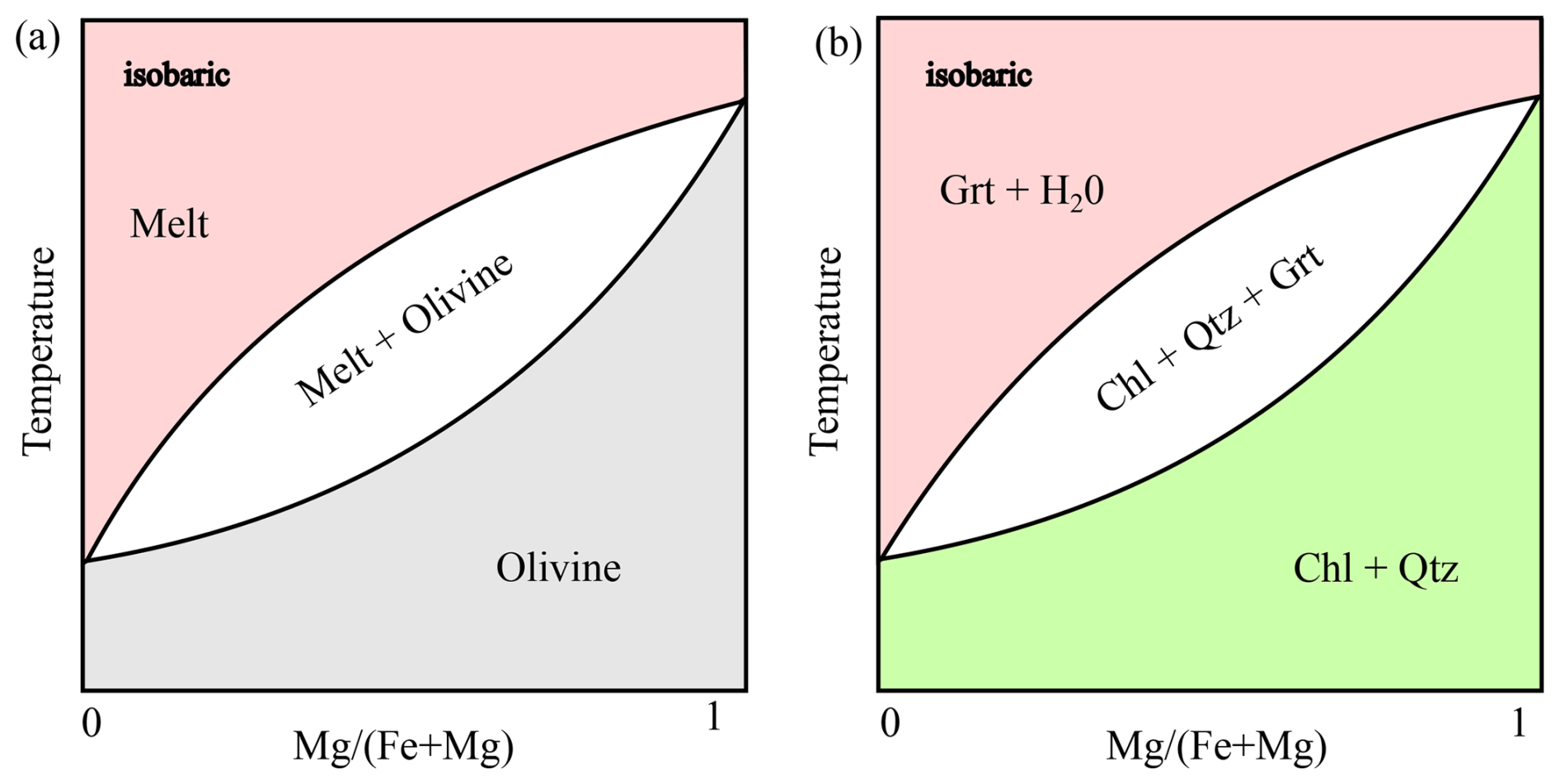
Figure 1 Schematic drawings of (a) magmatic and (b) metamorphic binary phase-diagram sections. Such diagrams can be utilized to predict the equilibrium composition of the coexisting phases in Eq. (18).

2.3.1 Regridding procedure and moving boundary treatment

For cases with non-zero interface velocity, the interface needs to move according to the reaction velocity v_a. To include this effect, we advect the interface at each step before the solution of the diffusion equation. In this case, the mutual interface moves by a distance ${\mathit{\kappa }}_{\mathrm{1}}\mathrm{\Delta }{x}_a^A=v_a\mathrm{\Delta }{t}_{\mathrm{adv}}$, where κ₁ is a constant smaller than 1.0 (here 0.99). The choice of κ₁ is made to avoid numerical instabilities. Since we are considering a fully implicit approach for the diffusion problem (Eq. 6), our diffusion timestep can be larger than the traditional CFL condition. However, keeping it smaller than ∼50 times $\mathrm{\Delta }{t}_{\mathrm{diff}}=\mathrm{\Delta }{x}_k^{A^{\mathrm{2}}}/\max (D^{\mathrm{A}},D^{\mathrm{B}})$ seems to provide stable results and accurate time integration. However, in cases where Δt_adv<Δt_diff, we consider Δt_adv as the appropriate timestep. In cases where $\mathrm{50.0}\cdot \mathrm{\Delta }{t}_{\mathrm{diff}}\le \mathrm{\Delta }{t}_{\mathrm{adv}}$, we use $\mathrm{50.0}\cdot \mathrm{\Delta }{t}_{\mathrm{diff}}\cdot \mathit{\text{CFL}}$ as a maximum timestep, where CFL is a number smaller than 1.0. The previous choice of parameters can change according to the requirements of the problem.

Having a suitable timestep Δt allows the movement of the boundary by v_aΔt which augments the computational grid by one point in order to be able to resolve the new interface exactly. With the augmented new interface location, we can implement the boundary conditions by using the appropriate interface compositions together with the Stefan condition. The final system of equations (including diffusion and interface boundary conditions) can be solved with standard linear solvers. The previous approach will lead in the net increase of the computational grid points, and it is not computationally efficient. For this reason, we apply a regridding procedure where we interpolate the previously calculated solution in a new grid that keeps the number of computational points and the numerical resolution constant. The regridding approach utilizes the interpolation via Piecewise Cubic Hermite Interpolating Polynomials (PCHIP; Kahaner et al., 1989). This interpolation approach seems to provide better results when it comes to overall mass conservation compared to simple linear or high-order polynomial interpolation. In summary, the combination of regridding together with PCHIP interpolation maintains accuracy and it is computationally efficient since it does not increase the size of the problem during the calculations.

2.3.2 Total mass-balance formulation

The previous approach in modelling the moving boundary utilizes Stefan condition (Appendix B) to ensure that mass balance is conserved at the interface. In cases where the diffusivity of one of the materials is much larger than the other (i.e., D^B≫D^A), and the mass flux at the outer boundaries is zero, then we can assume that material B is homogenized much faster if the timestep of the process is significantly larger than the characteristic diffusion time $\mathrm{d}{x}^{\mathrm{2}}/D^B$. In that limiting scenario, we can use a predefined growth velocity v_a and the total mass balance to construct a closed system of equations. The total mass content M^tot in our model is the sum of the masses of phases A, B and can be calculated via the following form:

$$\begin{array}{}\text{(19)}& \begin{array}{rl}{M}^{\mathrm{tot}}& =M^A+M^B=\underset{\mathrm{0}}{\overset{V\left(S\right)}{\int }}{\mathit{\rho }}^A{C}^A(t,V(x\left)\right)\mathrm{d}V\\ & +\underset{V\left(S\right)}{\overset{V\left(L\right)}{\int }}{\mathit{\rho }}^B{C}^B(t,V(x\left)\right)\mathrm{d}V\end{array}\end{array}$$

where V(x) is the appropriately chosen volume function (planar, cylindrical, spherical) used to calculate the total mass amount and S is the location of the interface as before. In the case of Eq. (19) C represents the mass fraction, for the cases when concentrations are used, ρ^A, ρ^B can be set to unity. The previous equation is solved using the trapezoid rule at every timestep together with a distribution coefficient as shown in Eqs. (16) and (18).

3 Computational results and benchmarks

In the following parts we present some calculated examples as results. All cases shown below are calculated using the m-refinement approach. In addition, we have considered some limiting cases that have known analytical solutions. For each example, we first describe the specific model configuration followed by the presentation of the results. The package contains more examples than we present here (https://github.com/AnStroh/MovingBoundaryMinerals.jl, last access: 2 December 2025; visit the GitHub repository for more information; Zenodo: Stroh et al., 2025). Detailed information on the respective input parameters can be found in the corresponding tables.

3.1 Intracrystalline diffusion

The first two examples, A1 and A2, consider the limiting case of pure intracrystalline diffusion, as for example in linear-, trace-element diffusion in crystals at constant P−T conditions. Example A1 assumes an initial profile created by a combination of five harmonic functions (eigenfunctions) in a homogenous material, a planar geometry and outer boundary conditions where the composition is constant (Dirichlet) through time. In this example, the diffusion coefficient D is considered constant. Table 1 summarizes all input values. The analytical solution of the diffusion profile is given by:

$$\begin{array}{}\text{(20)}& C(x,t)=\sum _m\exp \left({\displaystyle \frac{-m^{\mathrm{2}}{\mathit{\pi }}^{\mathrm{2}}Dt}{L^{\mathrm{2}}}}\right)A_m\sin \left({\displaystyle \frac{m\mathit{\pi }x}{L}}\right)\end{array}$$

and the initial conditions can be evaluated by setting t to zero in Eq. (20). Figure 2 shows a comparison between the analytical solution and the numerical model considering a single phase. The results show the agreement between the analytical and the numerical solutions.

Table 1 Summary of all input parameters for example A1. The parameters have the same names as in the code.

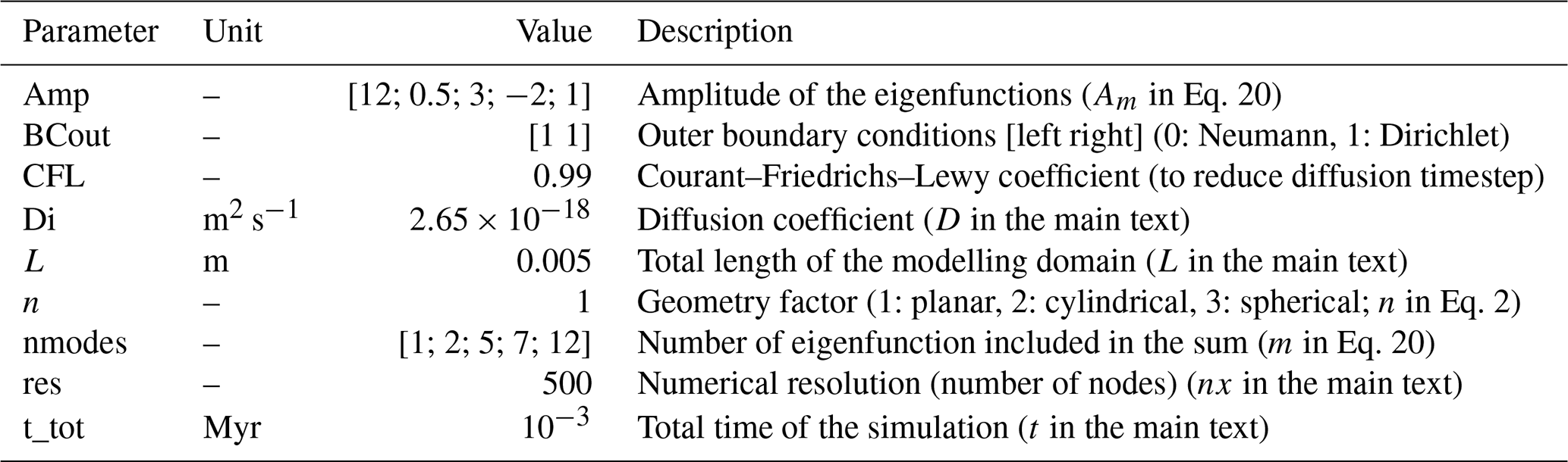
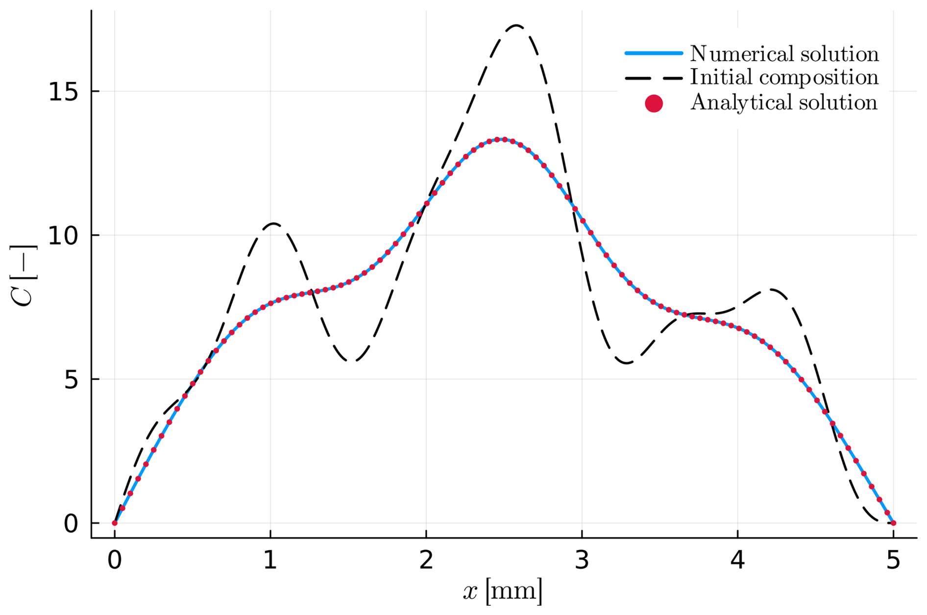
Figure 2 Example A1: simple intracrystalline diffusion within a planar crystal. The initial profile (dashed black line) and the analytical solution (red dots) were calculated using Eq. (20). The numerical solution is presented as the blue solid line.

Example A2 has a similar model configuration as example A1. However, in this case, we consider a spherical geometry with zero as initial condition and unity at the outer boundary (Dirichlet condition). The innermost boundary condition (at x=0) is of Neumann type (with no flux) due to the symmetry of the problem. Table 2 shows all input parameters needed to calculate A2. Figure 3 displays the resulting numerical solution and the corresponding analytical solution of the composition profile. Both solutions give the same result. The analytical solution for the example A2 can be found in Crank (1975; chap. 6.3.1) and it is summarized in the following Eqs. (21) and (22):

$$\begin{array}{}\text{(21)}& {\displaystyle }& {\displaystyle }C(\mathrm{0},t)=\mathrm{1}+\mathrm{2}\sum _{i=\mathrm{1}}^{\mathrm{\infty }}(-\mathrm{1}{)}^i\exp \left({\displaystyle \frac{-i^{\mathrm{2}}{\mathit{\pi }}^{\mathrm{2}}Dt}{L^{\mathrm{2}}}}\right)\text{(22)}& {\displaystyle }& {\displaystyle }C(x,t)=\mathrm{1}+{\displaystyle \frac{\mathrm{2}L}{\mathit{\pi }x}}\sum _{i=\mathrm{1}}^{\mathrm{\infty }}{\displaystyle \frac{(-\mathrm{1}{)}^i}{i}}\sin \left({\displaystyle \frac{i\mathit{\pi }x}{L}}\right)\exp \left({\displaystyle \frac{-i^{\mathrm{2}}{\mathit{\pi }}^{\mathrm{2}}Dt}{L^{\mathrm{2}}}}\right)\end{array}$$

where Eq. (21) provides the solution for the centre of the crystal (x=0) and Eq. (22) provides the solution for x>0.

Table 2 Summary of all input parameters for example A2. The parameters have the same names as in the code. Descriptions of previously defined parameters can be found in Table 1.

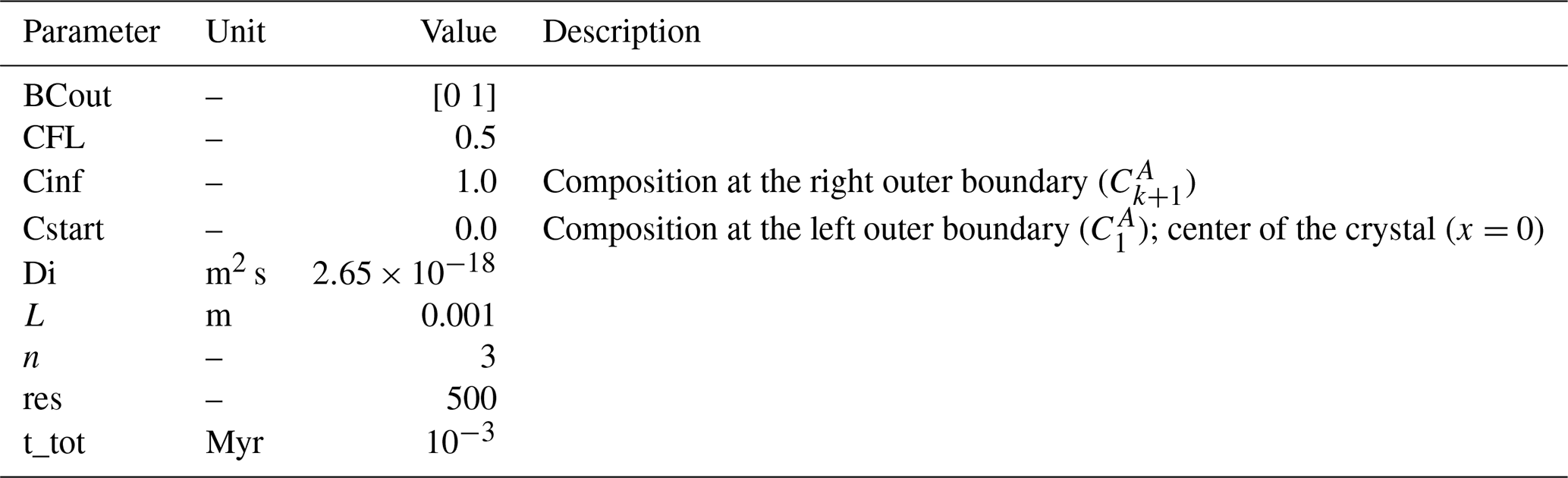
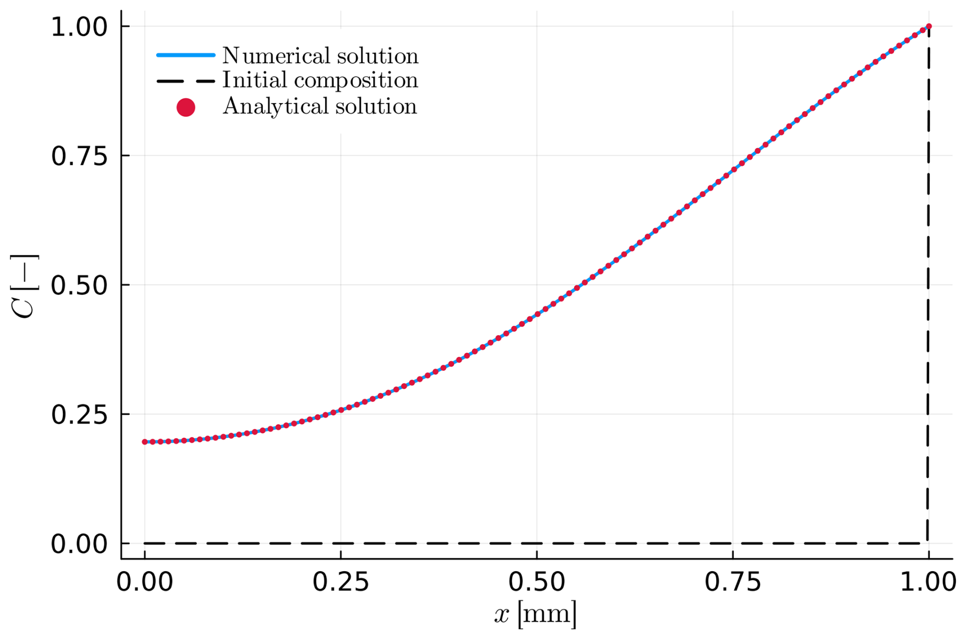
Figure 3 Example A2: simple intracrystalline diffusion in a spherical crystal. The initial profile (dashed black line) shows a homogeneous sphere with initially a different surface composition (at x=1.0). The numerical solution is presented as the blue solid line, while the red dots depict the analytical solution.

3.2 Intercrystalline diffusion (diffusion couple)

The previous models show the comparison of analytical solutions with the numerical solutions for a homogeneous material. In our models, we are mostly interested on the intercrystalline exchange and the compositional gradients that develop across materials with different properties. The method for solving the intercrystalline exchange is described in the Methods section and will not be repeated here.

A simple test that we can use to check for the accuracy of our diffusion-couple approach is to consider a diffusion couple in spherical geometry where the two domains (A and B) are treated separately but have identical diffusivities and their interface composition is given by Eq. (16) at the limit where K_D=1.0 (example B1). We can consider that the initial condition is zero for all domains and we can set the outer boundaries (at x=0 and x=1.0) as in example A2. Under these assumptions, the analytical solution described in Eqs. (21) and (22) is applicable. The parameters for the model configuration are given in Table 3. Note that to resolve any compositional gradients across the interface we can choose to refine the grid at the interface region. Figure 4 shows that the analytical solution matches the numerical solution and indeed it remains continuous at the interface as a consequence of setting K_D=1.0.

Table 3 Summary of all input parameters for example B1. The parameters have the same names as in the code. Descriptions of previously defined parameters can be found in Tables 1 and 2.

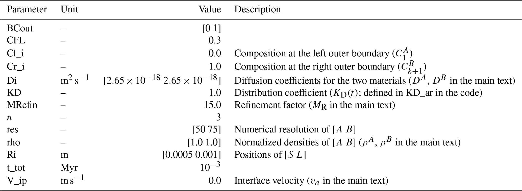
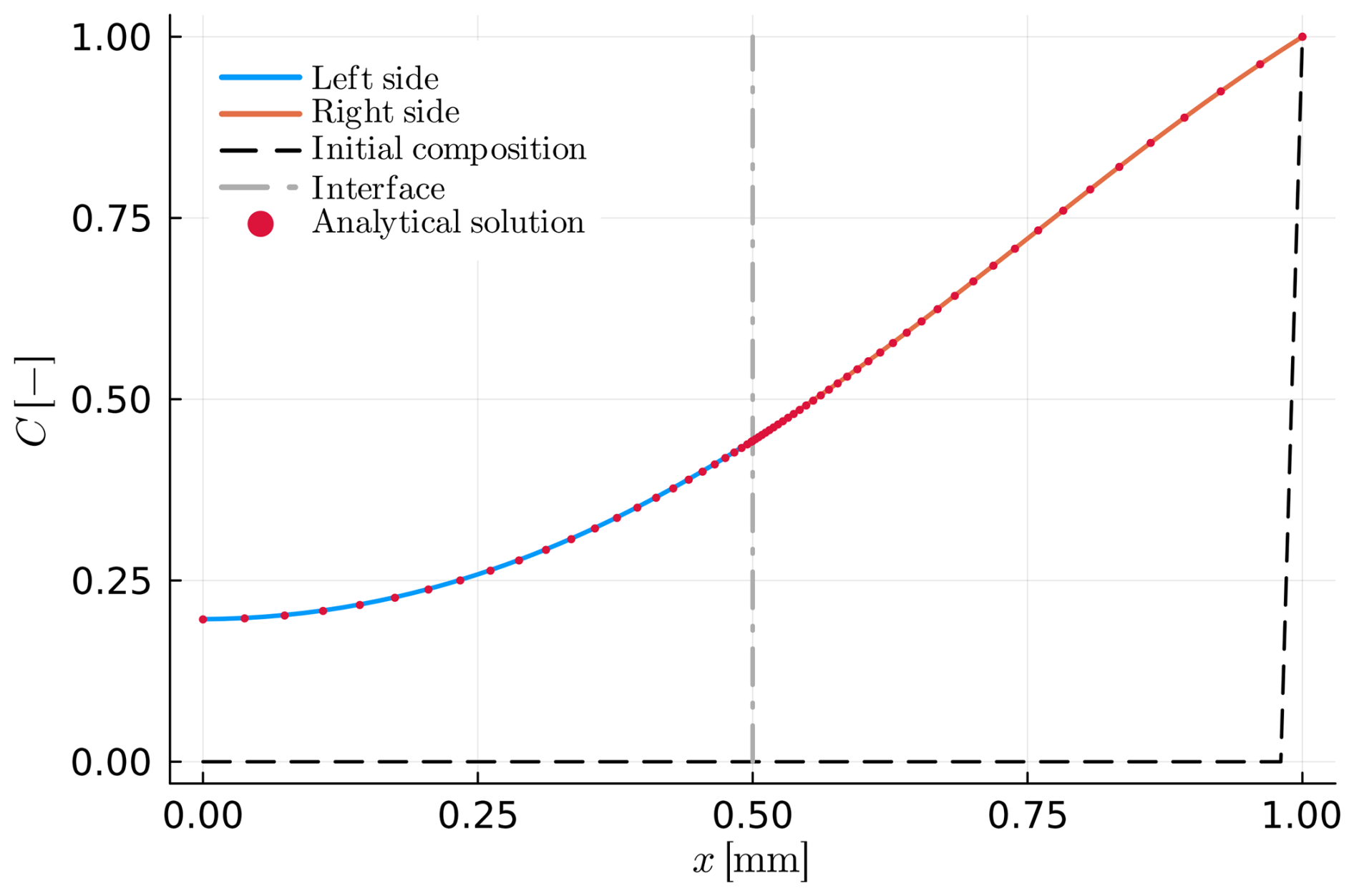
Figure 4 Example B1: intercrystalline diffusion within a spherical diffusion couple. Both parts have the same material properties, whereby the blue and orange lines refer to the left and the right side (numerical solutions). The initial profile (dashed black line) shows an initially homogeneous sphere with a different surface composition (x=1.0). The analytical solution is indicated using red dots. The interface position can be recognized by the dashed-dotted grey line at x=0.5.

In a similar approach as for the example B2, we can calculate an example where the diffusion coefficient changes through time following Eq. (3). The specific model parameters for this example are given in Table 4. In such a way, we can test for the accuracy of the time-integration scheme in our model. To proceed, we will consider an example where the temperature cools down with a constant rate from 1273 to 1073 K within two thousand years. The previous cooling path defines a function T(t) that can be used to express the diffusivity as a composite function of time (D(T(t))). For such problems Crank (1975) provides an analytical solution using a time-transformation technique (Crank, 1975; chap. 7). The time-transformation technique can be used to convert the non-isothermal problem into an isothermal one by calculating the following integral:

$$\begin{array}{}\text{(23)}& \mathit{\zeta }\left(t\right)=\underset{\mathrm{0}}{\overset{t}{\int }}\stackrel{\mathrm{̃}}{D}\left(t^{\prime }\right)\mathrm{d}{t}^{\prime }\end{array}$$

where $\stackrel{\mathrm{̃}}{D}\left(t\right)=D\left(T\right(t\left)\right)$ and t is time. Then, the solution of the time-dependent problem reduces to the solution of the following diffusion equation:

$$\begin{array}{}\text{(24)}& {\displaystyle \frac{\partial \stackrel{\mathrm{̃}}{C}}{\partial \mathit{\zeta }}}={\displaystyle \frac{\partial }{\partial x}}\left({\displaystyle \frac{\partial \stackrel{\mathrm{̃}}{C}}{\partial x}}\right)\end{array}$$

for which, analytical solutions exist as shown in the previous examples and in the literature (e.g., Perchuk and Philippot, 2000). In our case (example B2) we consider the analytical solution given by Eqs. (21) and (22) at the limit where t=ζ and D=1.0. The integral in Eq. (23) is solved numerically using the trapezoidal rule. Figure 5 shows that the solutions obtained numerically (via direct time integration) and analytically (via time transformation) are matching.

Table 4 Summary of all input parameters for example B2. The parameters have the same names as in the code. Descriptions of previously defined parameters can be found in Tables 1–3.

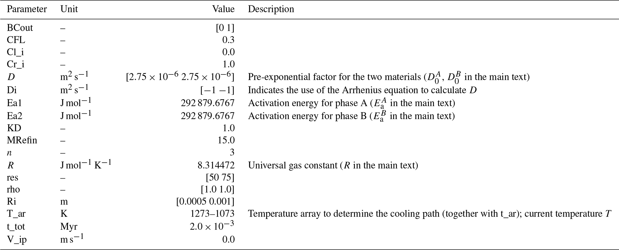
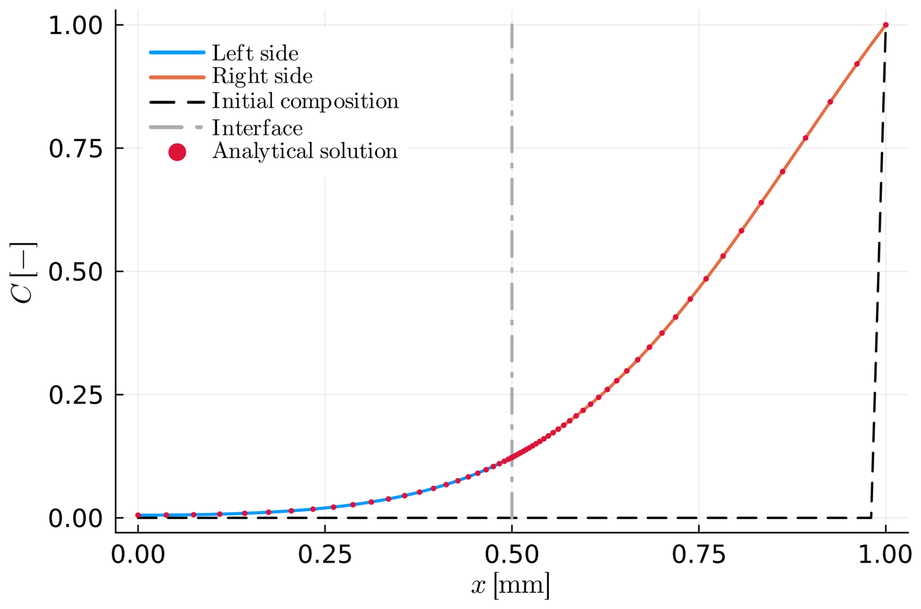
Figure 5 Example B2: diffusion within a spherical diffusion couple for the case of time-evolving diffusivity. Both parts have the same material properties and K_D=1.0. The blue and orange lines refer to the left and the right side (numerical solutions). The initial profile (dashed black line) shows an initially homogeneous sphere with a different surface composition. The numerical solutions are presented as blue and orange solid lines, while the red dots depict the analytical solution.

3.3 Crystal growth

In the previous examples, we showed cases where the interface is not moving (v_a=0.0). Our package can also be used to simulate crystal growth/dissolution. In the case where the diffusion of the growing solid is significantly smaller compared to its surrounding (D^A≪D^B), then we can approximate the composition distribution as a case of Rayleigh fractionation (Hollister, 1966). The previous assumption seems appropriate when large crystals grow within a fluid or a fine-grained, fast-diffusing matrix. To model this limit, we also considered the case where the diffusion timescale is much smaller than the reaction timescale. The ratio of the two timescales defines the Peclet number as shown below (e.g., Burg and Moulas, 2022; their Appendix B):

$$\begin{array}{}\text{(25)}& Pe={\displaystyle \frac{\mathit{\text{d}}{t}_{\mathrm{diff}}}{\mathit{\text{d}}{t}_{\mathrm{adv}}}}={\displaystyle \frac{\mathit{\text{d}}x\cdot v_a}{D}}\end{array}$$

where dx in Eq. (25) indicates the material replaced/formed by the reaction. In that limit, the analytical expressions for Rayleigh fractionation reduce to:

$$\begin{array}{}\text{(26)}& {\displaystyle }& {\displaystyle \frac{C^B}{C_{\mathrm{0}}^B}}={\left(\mathrm{1}-{\displaystyle \frac{M^A}{M_{\mathrm{0}}^A}}\right)}^{K_{\mathrm{D}}-\mathrm{1}}\text{(27)}& {\displaystyle }& {\displaystyle }{C}^A=K_{\mathrm{D}}\cdot C^B\end{array}$$

Equations (26) and (27) describe the boundary compositions of the finite reservoir and of the solid during the crystallization. However, because of the relatively slow diffusivity of the solid, the boundary composition of the solid is preserved as part of the chemical zonation. Thus, we can use Eqs. (26) and (27) to test our code at the limit where the diffusivity of the two materials is different, and the growth process is much faster compared to the diffusion in the slowest phase. In this case, we considered the instantaneous interface equilibrium (Eq. 16) and the flux balance using the Stefan condition (Eq. 18) to form a closed system of equations. Example B4 shows the good agreement between the analytical and numerical solution of the compositional distribution in the case of a growing crystal with a finite growth velocity (Fig. 6). Table 5 summarizes the input parameters of the model.

Table 5 Summary of all input parameters for examples B4 and C1. The parameters have the same names as in the code. Non-dimensional parameters are used. Descriptions of previously defined parameters can be found in Tables 1–4.

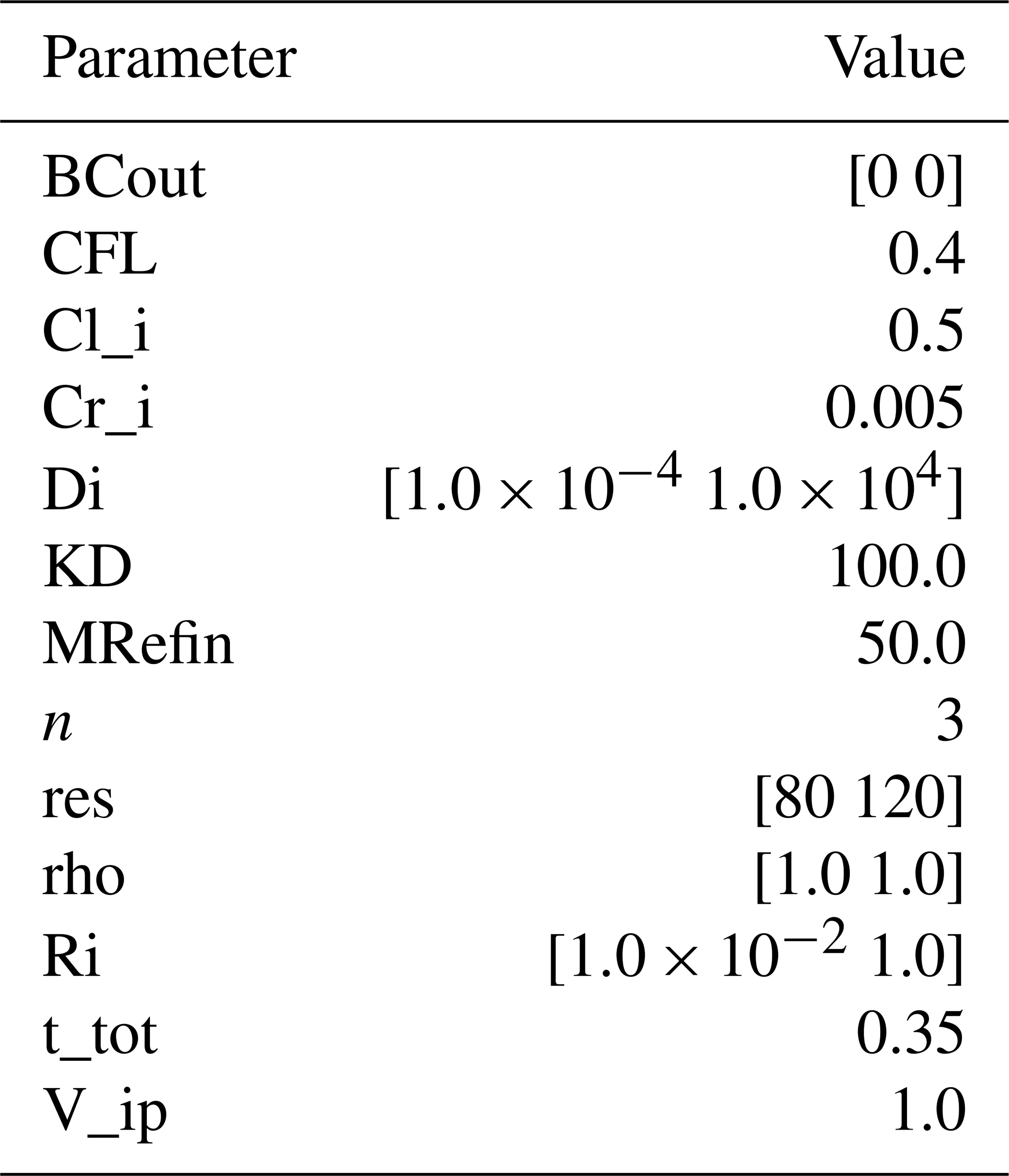
Figure 6 Example B4: spherical crystal growth due to Rayleigh fractionation in a growth and diffusion couple with D^A≪D^B. (a) The blue solid line depicts the composition of the growing crystal, while the solid orange line shows the composition within the melt reservoir. The grey dashed-dotted line presents the interface position in the compositional profile. The distribution coefficient is considered constant K_D=100.0. (b) Numerical and analytical solution of the solid interface as a function of the solid fraction.

Another limiting case that can be modelled is the case where D^A≪D^B but, this time, the growth of phase A and the diffusion process in B are of similar timescales (example B5). In the case where the growing crystal (A) is much smaller than the surrounding (B) we can use the analytical solution of Smith et al. (1955) for the segregation of an alloy from an impure melt in a planar geometry (Eqs. 28 and 29). This solution considers the growth of a crystal in an infinite medium and has already been applied to analyse results of kinetic disequilibrium processes including diffusion of trace elements within a crystal-melt system (Watson and Müller, 2009). Equation (28) predicts the composition within the reservoir (for $\widehat{x}>\mathrm{0}$).

$$\begin{array}{}\text{(28)}& \begin{array}{rl}& C^B(\widehat{x},t)=C^B(\widehat{x},\mathrm{0})\\ & \left\{\begin{array}{l}\mathrm{1}+\frac{\left(\mathrm{1}-K_{\mathrm{D}}\right)}{\mathrm{2}{K}_{\mathrm{D}}}\exp \left(-\frac{v\cdot \widehat{x}}{D^B}\right)\cdot \mathrm{erfc}\left(\frac{\sqrt{\frac{\mathrm{1}}{t\cdot D^B}}\left(\widehat{x}-v\cdot t\right)}{\mathrm{2}}\right)\mathrm{\dots }\\ -\frac{\mathrm{1}}{\mathrm{2}}\mathrm{erfc}\left(\frac{\sqrt{\frac{\mathrm{1}}{t\cdot D^B}}\left(\widehat{x}+v\cdot t\right)}{\mathrm{2}}\right)+\frac{\left(\mathrm{1}-K_{\mathrm{D}}\right)}{\mathrm{2}}\mathrm{\dots }\\ \cdot \left(\frac{\mathrm{1}}{\left(\mathrm{1}-K_{\mathrm{D}}\right)}-\frac{\mathrm{1}}{K_{\mathrm{D}}}\right)\exp \left(-\left(\mathrm{1}-K_{\mathrm{D}}\right)\frac{v}{D^B}\left(\widehat{x}+K_{\mathrm{D}}v\cdot t\right)\right)\mathrm{\dots }\\ \cdot \mathrm{erfc}\left(\frac{\sqrt{\frac{\mathrm{1}}{t\cdot D^B}}\left(\widehat{x}+\left(\mathrm{2}{K}_{\mathrm{D}}-\mathrm{1}\right)v\cdot t\right)}{\mathrm{2}}\right)\end{array}\right\}\end{array}\end{array}$$

where erfc( ) is the complementary error function and $\widehat{x}$ is related to the spatial coordinate as follows:

$$\begin{array}{}\text{(29)}& \widehat{x}=x-S\end{array}$$

Our calculated example B5 (Fig. 7) shows an excellent agreement between the numerical and analytical solutions. Model parameters for example B5 can be found in Table 6.

Table 6 Summary of all input parameters for example B5. The parameters have the same names as in the code but in this case, non-dimensional parameters are used. Descriptions of previously defined parameters can be found in Tables 1–5.

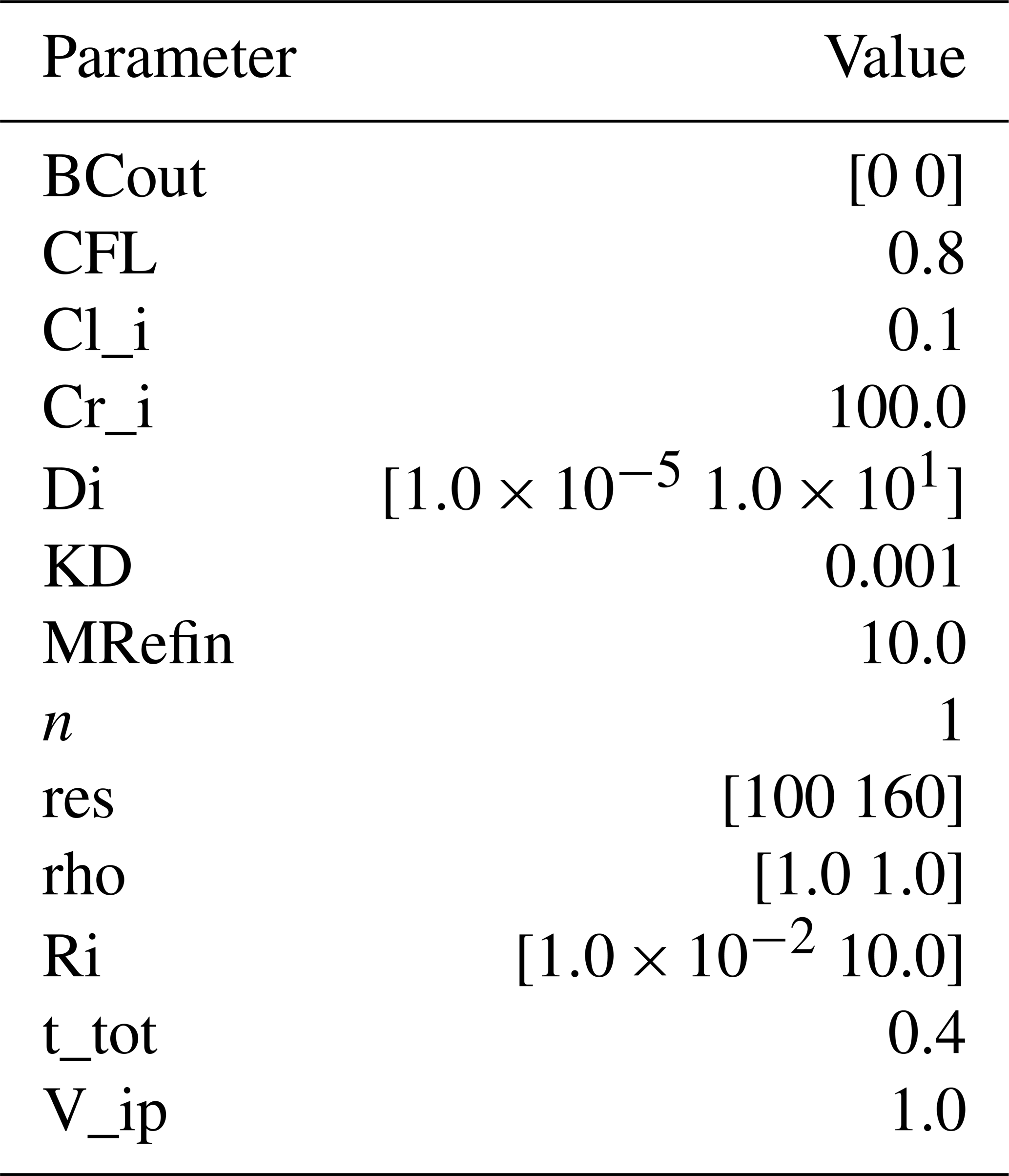
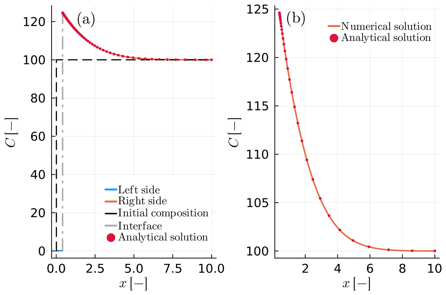
Figure 7 Example B5: growth of a crystal from a melt in a planar geometry. (a) Compositional profile of the growing crystal and the adjacent melt. The solid blue and orange lines show the diffusion couple. The black dashed line depicts the initial compositional profile, while the dashed-dotted grey line refers to the current position of the interface. The analytical solution of Smith et al. (1955) is shown in red dots. (b) Detailed view of the compositional profile of the melt showing modelled and analytical values.

In the case of crystal growth in a fast-diffusing medium, instead of the Stefan condition (Eq. 18), we can use the total mass balance (Eq. 19) to form a closed system of equations (example C1). In that case, the outer boundary conditions should be set to Neumann to prevent mass loss/gain during the process. The result of such a model is shown in Fig. C1 and the parameters used are the same as in Table 5. Figure C1 closely resembles Fig. 6 in the sense that it also compares well with the analytical solution for Rayleigh fractionation.

3.4 Simultaneous crystal growth/resorption and diffusion

The previous calculated examples show the limiting cases where at least one of the processes considered (growth or diffusion) was very fast compared to the others. In many natural examples, these processes may occur at the comparable rates. In the following examples we consider three different cases where diffusion and growth/resorption occur simultaneously. Examples B6 and B7 consider the cases of growth and resorption of phase A using the Stefan condition (Eq. 18) with a prescribed interface velocity (v_a). Example C2 is similar to B7, but for the case where the total mass-balance constraint (Eq. 19) is used in the calculation of the inner boundary conditions. All examples are calculated using non-dimensional quantities and only the relative ratios of diffusivities/reaction rates are important.

Although in the aforementioned examples reaction velocity is considered constant, natural reaction rates do not have to remain constant and can change according to temperature, reaction overstepping etc. Therefore, having a method that can consider arbitrary rates for the reaction rate allows the extension of our formulation to more elaborate cases. Furthermore, the distribution coefficient does not have to remain constant in time either. In the following examples, we consider cases where the distribution coefficient changes with time.

The first example that is considered in this section is example B6. In this example, the diffusivity of the two materials is similar, but not identical. In addition, we consider that the reaction velocity is positive (v_a>0), leading to the growth of A at the expense of B, whereas the distribution coefficient reduces from 50.0 to 25.0. The initial condition for both phases is considered homogeneous as in the equilibrium limit. More details on the model configuration can be found in Table 7. Figure 8 shows the evolution of the model after some time. The results of the simulation show that small compositional gradients develop on the side of the matrix (B). Additionally, the original growing crystal (A) exhibits evidence of chemical zoning that are qualitatively very similar to cases of pure growth (Figs. 6 and C1). Note that the “core” composition of A is distinctively different compared to the initial condition.

Table 7 Summary of all input parameters for example B6. The parameters have the same names as in the code but in this case, non-dimensional parameters are used. Descriptions of previously defined parameters can be found in Tables 1–6.

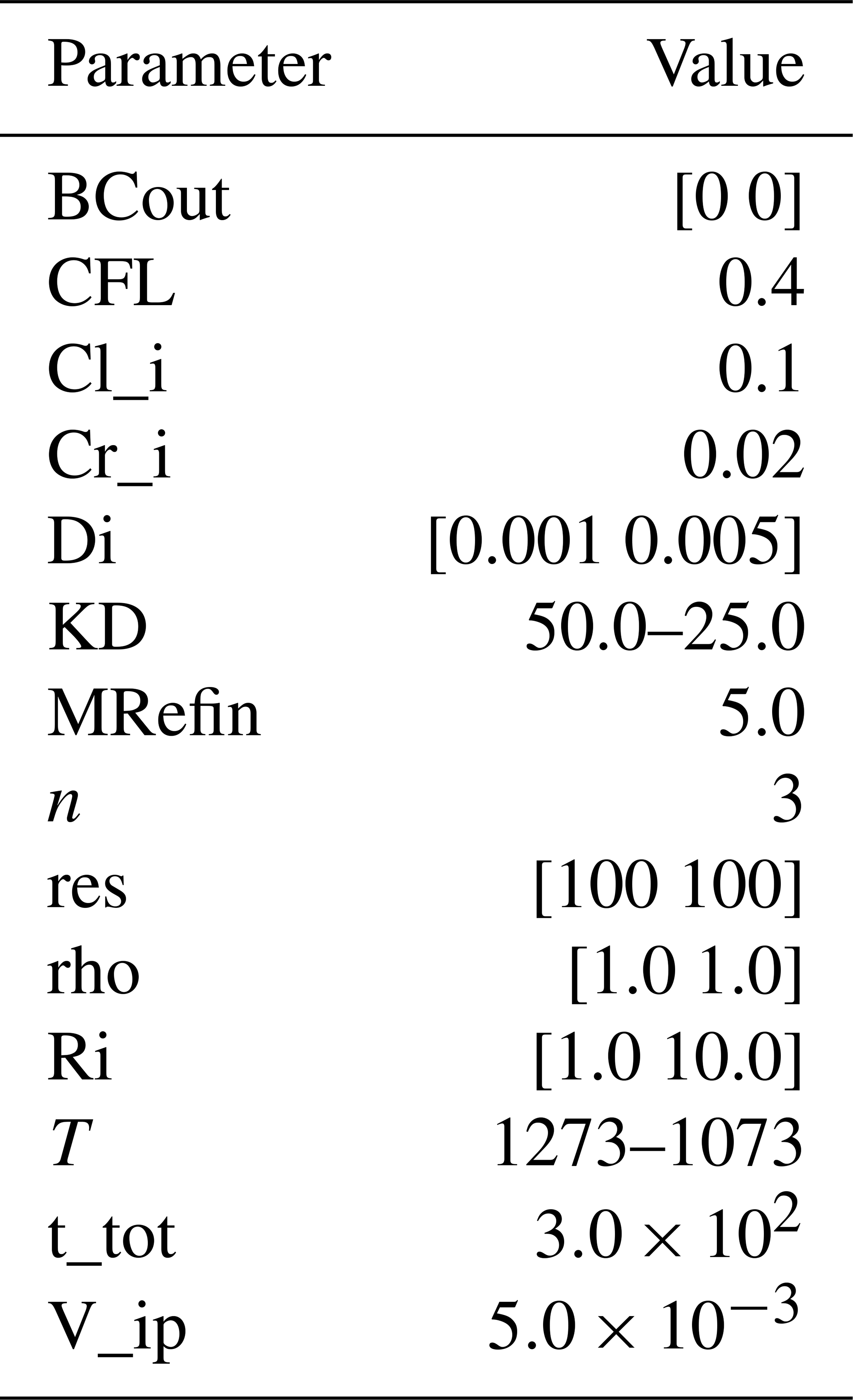
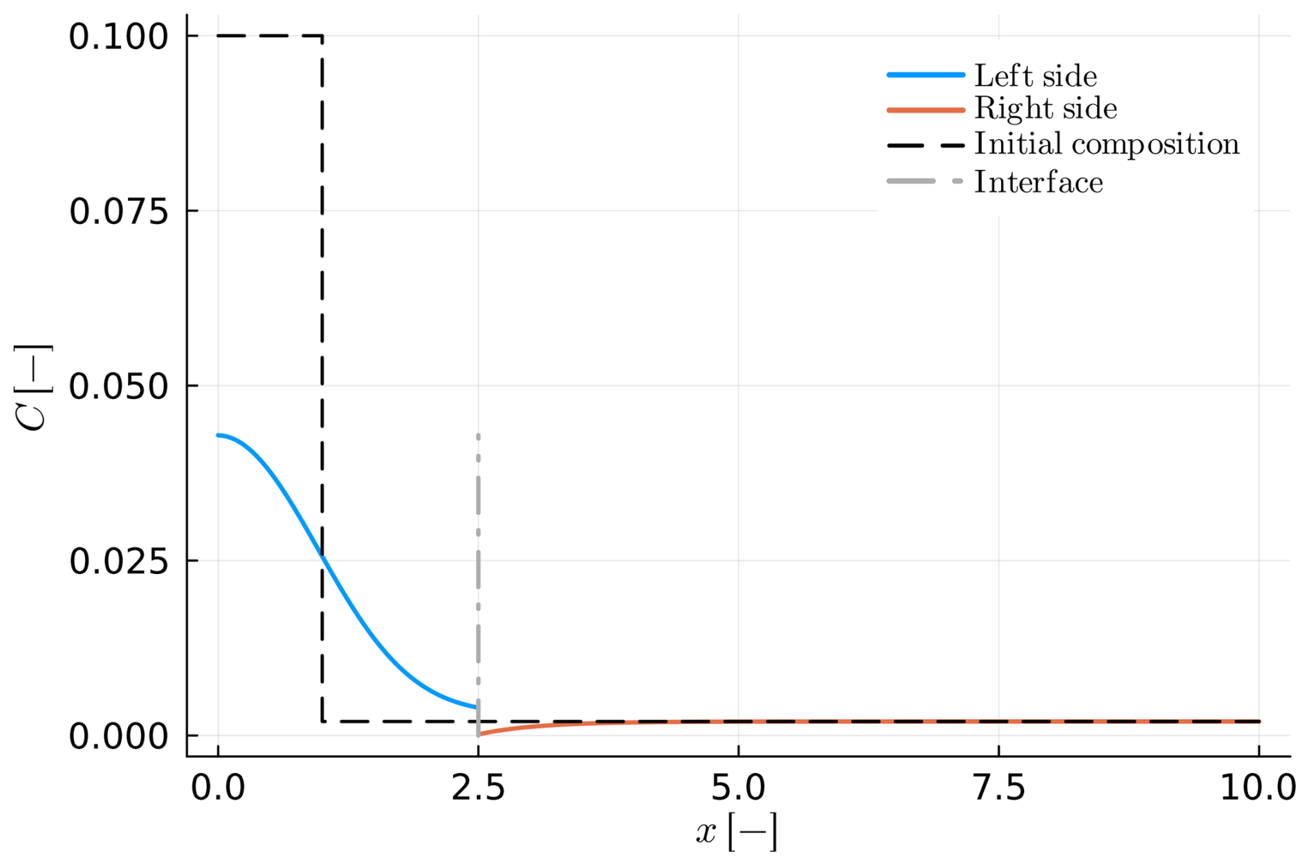
Figure 8 Example B6: growth of a spherical crystal in a diffusion couple (v_a>0). The solid blue and orange lines represent the composition in the diffusion couple after some finite time. The grey dashed-dotted line shows the current position of the interface, while the black dashed line represents the initial position of the interface.

Figure 9 shows a case where the reaction velocity is negative (v_a<0; resorption of A). The parameters in this example are almost identical to the parameters used in example B6. The main differences in this case (B7) are, (i) the negative reaction velocity, (ii) the initial size of crystal A, (iii) the distribution coefficient reduces from 20.0 to 10.0. More details on the parameters are found on Table 8. The compositional gradients at the side of the matrix are also observed in this case, however, the compositional gradients at the side of the consuming crystal are very pronounced, as it is expected for very compatible elements (e.g., Burg and Moulas, 2022; Kohn and Spear, 2000). Finally, Fig. C2 shows an example (C2) almost identical to the previous one (B7). The only difference in this case is that the inner boundary condition is solved via the total mass balance constraint (Eq. 19). The results are similar and converge to the results shown in Fig. 9.

Table 8 Summary of all input parameters for examples B7 and C2. The parameters have the same names as in the code but in this case, non-dimensional parameters are used. Descriptions of previously defined parameters can be found in Tables 1–7.

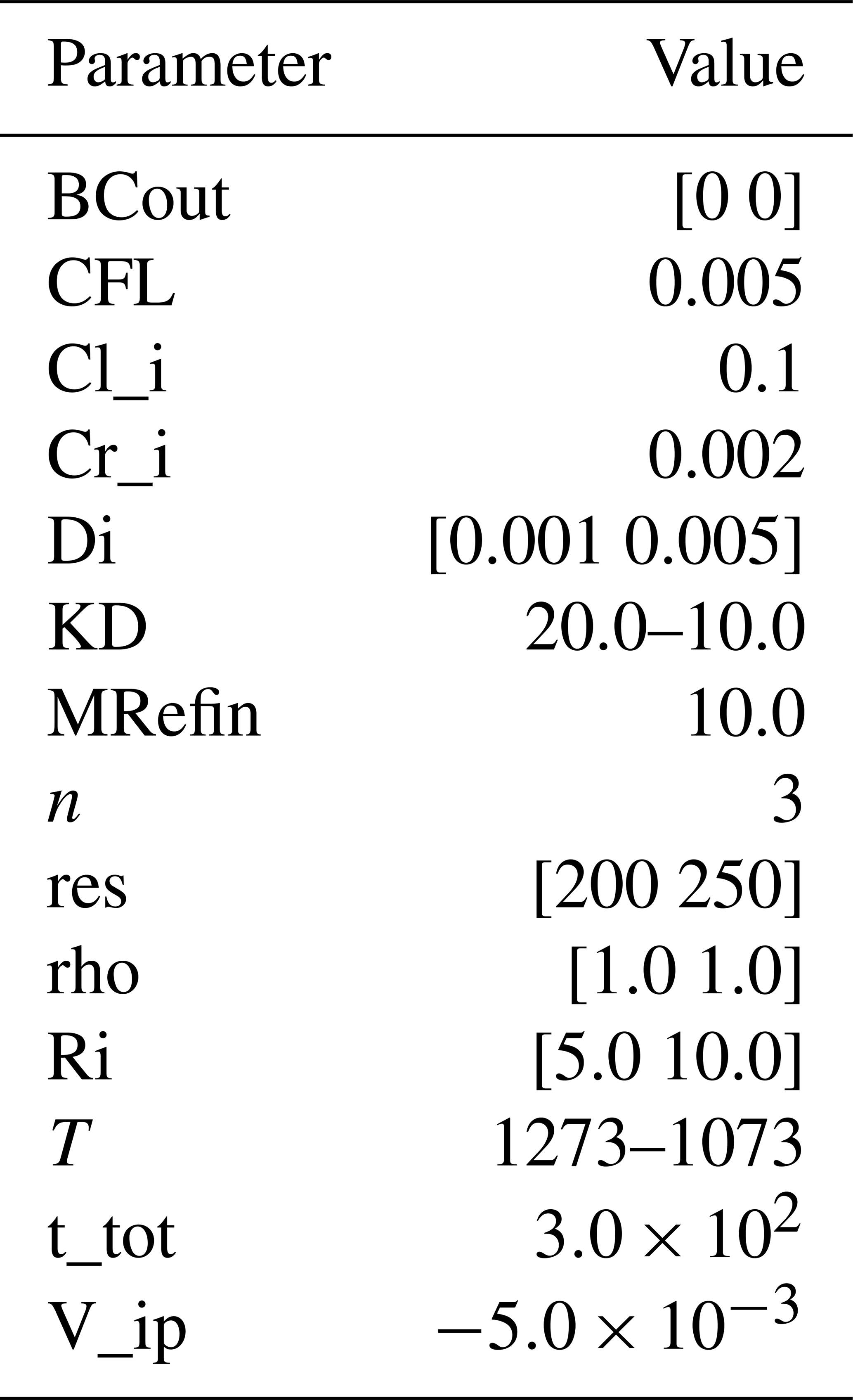
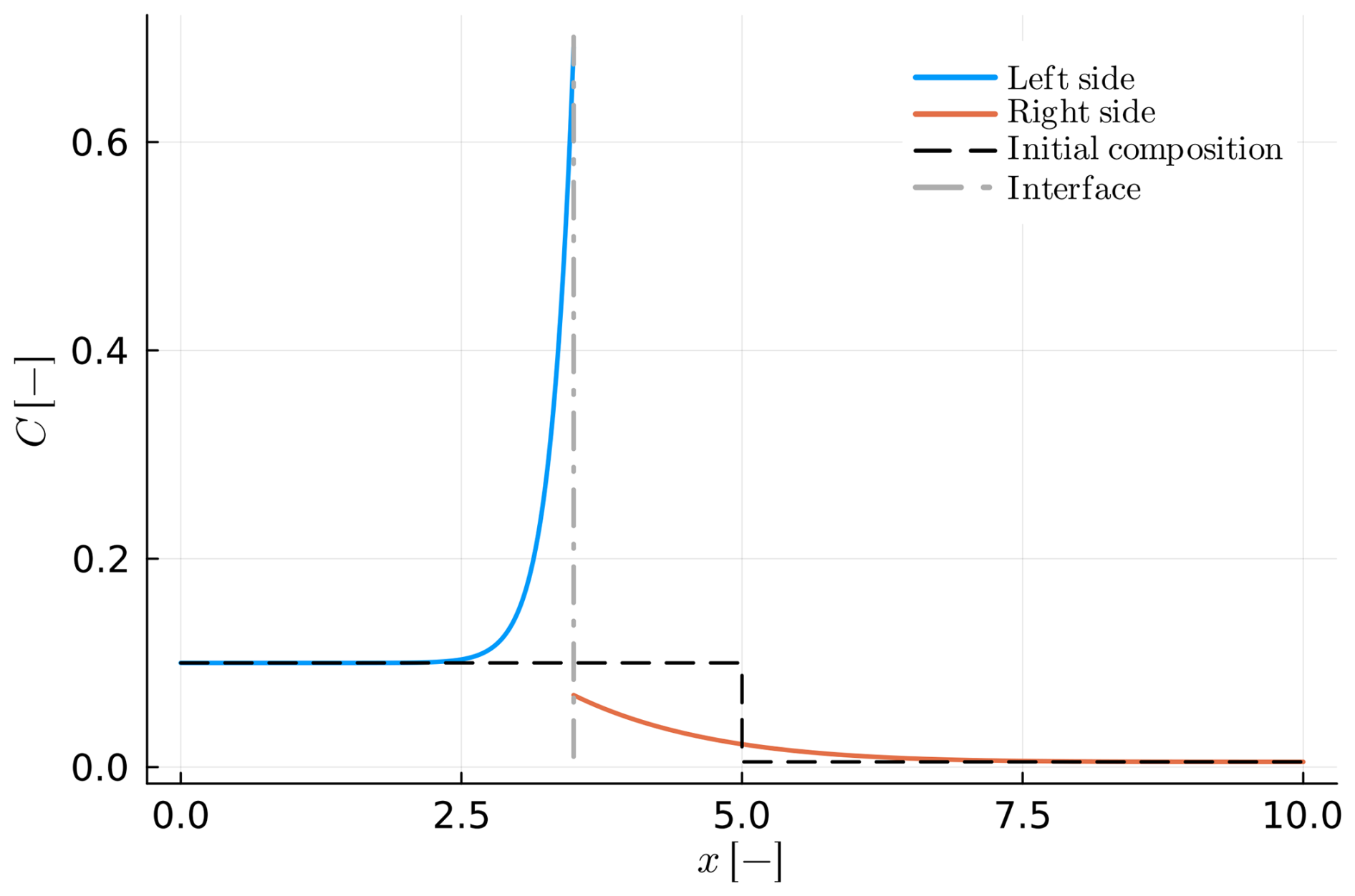
Figure 9 Example B7: similar to B6 (Fig. 8) but with negative reaction velocity (v_a<0). More details on the parameters used can be found at Table 8. The mass balance at the interface was calculated using the local flux balance (Eq. 18).

3.5 Diffusion-controlled crystal growth

In all previous examples, we have considered cases where the reaction velocity (v_a) was prescribed. In many natural cases, this velocity can be predicted if the thermodynamic properties of the two phases are known. One such case is the case of diffusion-limited growth where the reaction velocity is predicted from the equilibrium compositions of the interface (Balluffi et al., 2005; p. 504; Rubinsteĭn, 1971; p. 52). In that case, the equilibrium compositions in Eq. (18) can be evaluated from thermodynamic models (e.g., phase diagrams) and the velocity can be obtained by solving Eq. (18) with respect to v_a. As a working example, we consider a simplified case of olivine crystallization (example D1). In this example olivine is growing out of a melt that can be described using a binary component. In this case we consider $X_{\mathrm{Fe}}(\mathrm{Fe}/(\mathrm{Mg}+\mathrm{Fe})-\mathrm{molar}\mathrm{ratios})$ to describe the compositional evolution of the system. We have used Perplex (Connolly, 2005) to create a temperature-composition (T−X) phase-diagram section at constant pressure. The compositional variables can be fit using the following explicit forms

$$\begin{array}{}\text{(30)}& {\displaystyle }\begin{array}{rl}{\left.C^A\left(T\right)\right|}_{x=S^{-}}& =-\mathrm{6.46464}\times {\mathrm{10}}^{-\mathrm{7}}\times T^{\mathrm{2}}\\ & +\mathrm{0.00102}\times T+\mathrm{0.80653}\end{array}\text{(31)}& {\displaystyle }\begin{array}{rl}{\left.C^B\left(T\right)\right|}_{x=S^{+}}& =\mathrm{2.60617}\times {\mathrm{10}}^{-\mathrm{6}}\times T^{\mathrm{2}}\\ & -\mathrm{0.01002}\times T+\mathrm{9.79428}\end{array}\end{array}$$

where T is the temperature in K, and C should be the composition expressed in molar ratios. In this approach we prescribe a starting temperature, a final temperature and a cooling interval where the cooling rate is calculated and is considered constant. The initial composition of the phases is considered homogeneous. The directional diffusion coefficients (in m² s⁻¹) of olivine are calculated following the formulas provided by Dohmen and Chakraborty (2007a, b):

$$\begin{array}{}\text{(32)}& {\displaystyle }\begin{array}{rl}{\log }_{\mathrm{10}}\left(D_{\mathrm{001}}\right)=& {\log }_{\mathrm{10}}\left(D_{\mathrm{0}}\right)-\left(E_{\mathrm{a}}+\left(P-{\mathrm{10}}^{\mathrm{5}}\right)\cdot \mathrm{\Delta }V\right)\\ & \times (\mathrm{2.303}\cdot RT{)}^{-\mathrm{1}}+\mathrm{3}\cdot \left(X_{\mathrm{Fe}}-\mathrm{0.14}\right)\end{array}\text{(33)}& {\displaystyle }{\log }_{\mathrm{10}}\left(D_{\mathrm{100}}\right)={\log }_{\mathrm{10}}\left(D_{\mathrm{010}}\right)={\log }_{\mathrm{10}}\left(D_{\mathrm{001}}\right)-{\log }_{\mathrm{10}}\left(\mathrm{6.0}\right)\end{array}$$

P is the pressure in Pa, ΔV refers to the activation volume in m³ mol⁻¹ and $D_{\mathrm{001}}^A$, $D_{\mathrm{010}}^A$, $D_{\mathrm{100}}^A$ are the diffusion coefficients related to the different crystallographic axis of olivine. Equation (32) shows that the diffusion coefficient depends on composition, thus making the solution of the diffusion problem non-linear. Here, we linearize the problem by taking an average value of X_Fe in olivine. This is justified since, for the coupled problem, the difference in diffusivity between olivine and melt is orders of magnitude larger compared to the changes caused by the compositional dependence in olivine. Having Eqs. (32) and (33), the effective directional diffusion coefficient is calculated following Crank (1975; p. 7).

$$\begin{array}{}\text{(34)}& D^A=D_{\mathrm{001}}^A{\cos }^{\mathrm{2}}\left(\mathit{\alpha }\right)+D_{\mathrm{010}}^A{\cos }^{\mathrm{2}}\left(\mathit{\beta }\right)+D_{\mathrm{100}}^A{\cos }^{\mathrm{2}}\left(\mathit{\gamma }\right)\end{array}$$

The diffusivity of the silicate melt (phase B) is approximated by the formula given by Zhang et al. (2010; p. 332 their Eq. 19).

$$\begin{array}{}\text{(35)}& D^B=\exp \left(-\mathrm{7.92}-{\displaystyle \frac{\mathrm{26222}}{T}}\right)\end{array}$$

The remaining of the model parameters are given in Table 9.

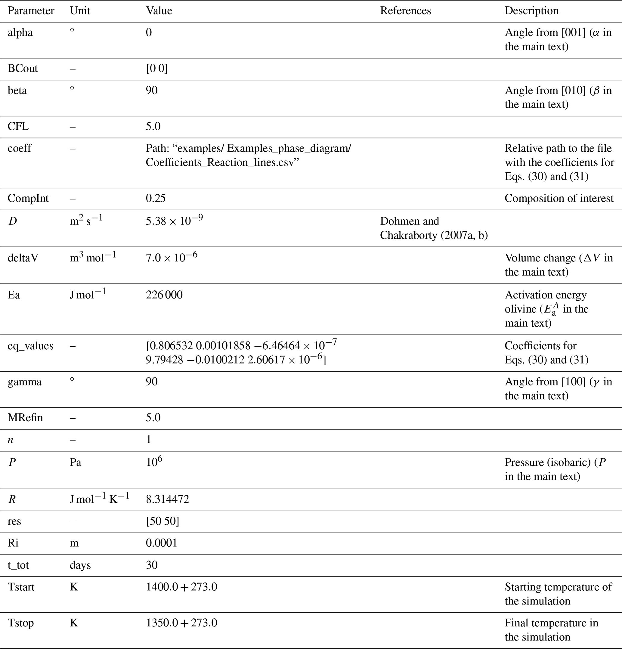
Table 9 Summary of all input parameters for example D1. Descriptions of previously defined parameters can be found in Tables 1–8.

The results of this model show that, with decreasing temperature, olivine is crystallized as expected, and compositional gradients evolve close to the interface. However, because of the significantly larger diffusivity of the melt, the compositional gradients at the side of the melt (x>S) are much smaller than within the crystal.

Figure 10 shows the results of diffusion-limited olivine growth. Figure 10a displays the compositional profile. The iron content increases in both phases, while the left phase, olivine, grows out of melt. This is consistent with the evolution in the phase diagram section (Fig. 10b). Figure 10b shows part of an isobaric phase-diagram section. The blue and red curves determine the liquidus and the solidus, which define the equilibrium composition of the melt and the olivine at the interface. During the whole simulation, the compositions at the interface agree between the modelled data and the phase diagram indicating the evolution of the binary system.

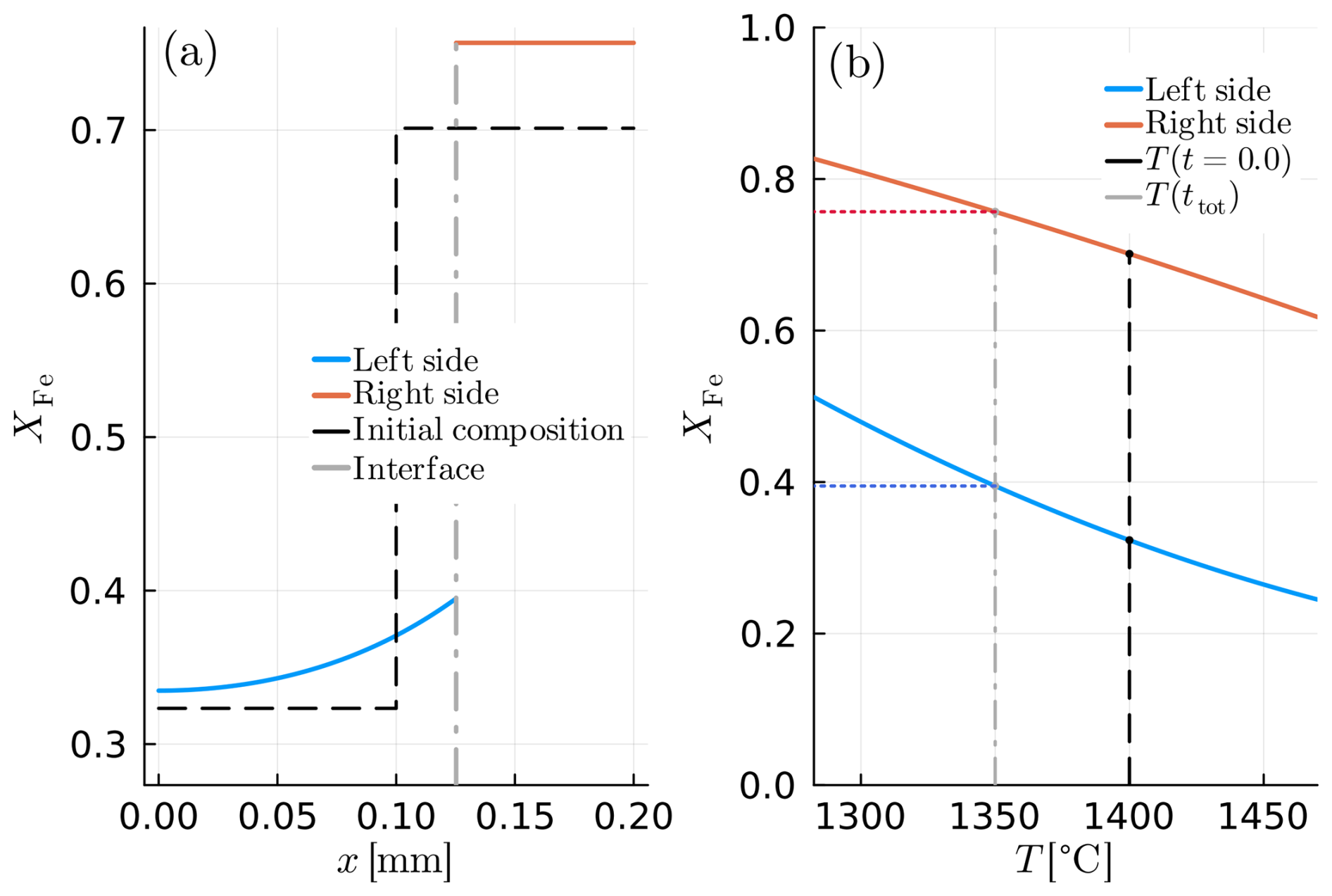
Figure 10 Example D1: diffusion-limited crystal growth of olivine. (a) Compositional profile of the diffusion couple, where the blue line refers to olivine and the red line depicts the melt. (b) Equilibrium boundary compositions. The coloured dashed lines show the exact composition of both materials at the interface at the end of the model. The grey dashed line shows the final temperature in the model.

4 Discussion and conclusions

We have presented MovingBoundaryMinerals.jl, a new software package, that can be used to model diffusion-controlled growth/resorption in mineral couples. The software has been written fully in Julia, it is openly available and allows for continuous integration. Our package can be used in various cases where mineral couples react, either via simple, exchange reactions or via mineral replacement (e.g., Eiler et al., 1992; Skora et al., 2006; Spear, 1991). The package utilizes a fully implicit method and has been tested for its accuracy in simulating cases with T(t)−P(t)-dependent diffusion coefficients and partition functions K_D(t), as it is required for geospeedometry applications (e.g., Lasaga, 1983; Ozawa, 1983). In addition, the package uses the finite element method with adaptive grid close to the interface of the diffusion couple. This approach offers improved resolution close to interface where the compositional gradients are sharper. We have tested the package versus various end-member cases that have known analytical solutions. Our results show good agreement with the calculated benchmarks and a good match of the numerical and analytical solutions close to the interface boundaries (Figs. 2–7).

In addition, we have presented calculated examples of diffusion/growth processes that are of petrological relevance (Figs. 8–10). In particular, Fig. 8 shows a case where simultaneous growth and diffusion produce a chemically zoned crystal which preserves some of its chemical zonation. The preserved zonation is the combined effect of growth and diffusion, and it is not related to the original zoning. However, we emphasize the result of this example since similar, bell-shaped profiles are typically used to infer prograde growth of metamorphic porphyroblasts (e.g., garnet) when diffusion is limited (e.g., Gaidies et al., 2008; Hollister, 1966). Our package can thus be used to test the former hypothesis and quantify the diffusion extend that occurred simultaneous or after mineral growth. Figures 9 and C2 show two similar cases of mineral resorption that causes an element enrichment at the edge of the mineral being consumed. The previous examples demonstrate that our approach can be used to investigate crystal growth and resorption rates in experiments and in metamorphic/magmatic systems. In particular, the sharp compositional gradients at crystal interfaces are very common in the metamorphic and magmatic petrology literature and can be used to infer effective cooling rates or element partitioning (e.g., Bindeman and Melnik, 2016; Burg and Moulas, 2022; Chu et al., 2018; Spear, 2014). However, the final compositional profile depends also on the diffusion properties of the matrix. By implementing two approaches, one using the local-mass-balance (Fig. 9) and one using the total-mass-balance constraint (Fig. C2), we can test cases where the diffusivity of the matrix is not infinitely fast. These approaches allow the modelling minerals being consumed in finite geochemical reservoirs. As a third example, we have presented a calculated case of olivine crystallization during cooling at conditions where diffusion in olivine is not negligible (Fig. 10). Our approach follows the classical Stefan problem and considers the cases of diffusion-limited growth. This approach was chosen since it converges to the right equilibrium limit and can be used in modelling the diffusion of a growing crystal in the laboratory or in nature. Note that, in these examples, the diffusion coefficients were considered to be composition independent, future additions in this package can include non-linear diffusion and interface kinetic processes that are not resolved in this work.

Appendix A: Derivation of diffusion and mass-balance relationships used in this study

The derivation of many equations used in this work is summarized in the following part. The following derivations largely follow the classic derivations described in De Groot and Mazur (1984). For a homogeneous substance (in 1 dimension) the conservation of mass reads:

$$\begin{array}{}\text{(A1)}& {\displaystyle \frac{\partial \mathit{\rho }}{\partial t}}+{\displaystyle \frac{\partial \left(\mathit{\rho }v\right)}{\partial x}}=\mathrm{0}\end{array}$$

where ρ is the total density in kg m⁻³, t is time in s, v is the velocity in the x direction (in m s⁻¹) and x is the spatial coordinate in m. For a multicomponent phase, having n different diffusing species, Eq. (A1) can be formulated for each species. The density of any species i relates to the total density as follows (e.g., De Groot and Mazur, 1984; their Eq. 6):

$$\begin{array}{}\text{(A2)}& \mathit{\rho }=\sum _{i=\mathrm{1}}^n{\mathit{\rho }}_i.\end{array}$$

For a non-reacting medium, the conservation of species i becomes:

$$\begin{array}{}\text{(A3)}& {\displaystyle \frac{\partial {\mathit{\rho }}_i}{\partial t}}+{\displaystyle \frac{\partial \left({\mathit{\rho }}_i{v}_i\right)}{\partial x}}=\mathrm{0}\end{array}$$

where v_i is the macroscopic velocity of the species i in the Eulerian reference frame. Summing up Eq. (A3) for species i from 1 to n, leads to Eq. (A1). The latter though requires that v is the barycentric velocity of the phase, that is:

$$\begin{array}{}\text{(A4)}& v=\sum _{i=\mathrm{1}}^n\left(C_i{v}_i\right)\end{array}$$

where C_i is the weight fraction (dimensionless) of the species i in the solution. By defining the macroscopic diffusive flux of species i with respect to the barycentric velocity, we can write Eq. (A3) as follows:

$$\begin{array}{}\text{(A5)}& {\displaystyle \frac{\partial {\mathit{\rho }}_i}{\partial t}}+{\displaystyle \frac{\partial \left({\mathit{\rho }}_{i}v\right)}{\partial x}}+{\displaystyle \frac{\partial \left({\mathit{\rho }}_i\left(v_i-v\right)\right)}{\partial x}}=\mathrm{0}.\end{array}$$

At this point, we can apply the product rule to the second term of Eq. (A5) to obtain the following relationship:

$$\begin{array}{}\text{(A6)}& {\displaystyle \frac{\partial {\mathit{\rho }}_i}{\partial t}}+v{\displaystyle \frac{\partial {\mathit{\rho }}_i}{\partial x}}+{\mathit{\rho }}_i{\displaystyle \frac{\partial v}{\partial x}}+{\displaystyle \frac{\partial \left({\mathit{\rho }}_i\left(v_i-v\right)\right)}{\partial x}}=\mathrm{0}\end{array}$$

where the previous can be written in a more compact form (using Lagrangian notation) as follows:

$$\begin{array}{}\text{(A7)}& {\displaystyle \frac{\mathrm{d}{\mathit{\rho }}_i}{\mathrm{d}t}}=-{\mathit{\rho }}_i{\displaystyle \frac{\partial v}{\partial x}}-{\displaystyle \frac{\partial {\mathrm{\Phi }}_i}{\partial x}}\end{array}$$

where Φ_i represents the mass-diffusion flux with respect to the barycentric velocity (Kuiken, 1994; his Eq. 4.55), and it is defined as follows:

$$\begin{array}{}\text{(A8)}& {\mathrm{\Phi }}_i={\mathit{\rho }}_i\left(v_i-v\right).\end{array}$$

At the Fickean limit, the flux is related to the concentration gradient, that can be reduced to:

$$\begin{array}{}\text{(A9)}& {\mathrm{\Phi }}_i=-D_i{\displaystyle \frac{\partial {\mathit{\rho }}_i}{\partial x}}\end{array}$$

with D_i being a positive constant (diffusion coefficient). By making use of Eqs. (A7) to (A9), Eq. (A6) can be written as:

$$\begin{array}{}\text{(A10)}& {\displaystyle \frac{\mathrm{d}{\mathit{\rho }}_i}{\mathrm{d}t}}+{\mathit{\rho }}_i{\displaystyle \frac{\partial v}{\partial x}}+{\displaystyle \frac{\partial {\mathrm{\Phi }}_i}{\partial x}}=\mathrm{0}.\end{array}$$

In addition, at the limit where the macroscopic velocity is zero (no advection), and the volumetric deformation is negligible, the previous reduces to the following familiar form:

$$\begin{array}{}\text{(A11)}& {\displaystyle \frac{\partial {\mathit{\rho }}_i}{\partial t}}=D_i{\displaystyle \frac{{\partial }^{\mathrm{2}}{\mathit{\rho }}_i}{\partial x^{\mathrm{2}}}}\end{array}$$

which is the classic form of the diffusion equation with ρ_i having units of mass per volume (kg m⁻³). In the same limit, where volumetric deformation is negligible the previous reduces to Eq. (1) of the main text:

$$\begin{array}{}\text{(A12)}& {\displaystyle \frac{\partial C_i}{\partial t}}=D_i{\displaystyle \frac{{\partial }^{\mathrm{2}}{C}_i}{\partial x^{\mathrm{2}}}}\end{array}$$

where C_i represents the weight fraction of the species involved, such equations are trivially used in petrological literature for single/multicomponent diffusion (e.g., Guo and Zhang, 2016). As a final note we would like to emphasize that, given the model assumptions (i.e., that the volumetric deformation is negligible), Eq. (A12) is equally valid if mol fractions are used. However, the latter should be used consistently with the original data that were used to fit the diffusion coefficient D_i.

Appendix B: Derivation of the flux balance conditions at the interface

Solving for the inner boundary condition of our diffusion couple requires that any imbalance in the boundary fluxes across the materials is balanced by the Stefan condition (e.g., Rubinsteĭn, 1971; his Eq. 2.3.5₇). This requires that:

$$\begin{array}{}\text{(B1)}& \begin{array}{rl}\left({\left.{\mathit{\rho }}^B{C}^B\right|}_{x=S^{+}}\right.& \left.-{\left.{\mathit{\rho }}^A{C}^A\right|}_{x=S^{-}}\right)v_a={\left.-{\mathit{\rho }}^B{D}^B{\displaystyle \frac{\partial C^B}{\partial x}}\right|}_{x=S^{+}}\\ & +{\left.{\mathit{\rho }}^A{D}^A{\displaystyle \frac{\partial C^A}{\partial x}}\right|}_{x=S^{-}}\end{array}\end{array}$$

where A, B indicate the phase at the left or right side respectively, v_a is the reaction velocity (Eq. 4) and we have omitted the component subscripts for clarity. The previous equation holds for any component i and it is similar to the Stefan condition in heat flow problems (Rubinsteĭn, 1971). Note that in cases of simple ion-exchange equilibrium, where the velocity of the interface is zero, the previous simplifies to:

$$\begin{array}{}\text{(B2)}& {\left.{\mathit{\rho }}^A{D}^A{\displaystyle \frac{\partial C^A}{\partial x}}\right|}_{x=S^{-}}={\left.{\mathit{\rho }}^B{D}^B{\displaystyle \frac{\partial C^B}{\partial x}}\right|}_{x=S^{+}}\end{array}$$

which can be also written as:

$$\begin{array}{}\text{(B3)}& {\left.D^A{\displaystyle \frac{\partial C^A}{\partial x}}\right|}_{x=S^{-}}={\left.{\displaystyle \frac{{\mathit{\rho }}^B}{{\mathit{\rho }}^A}}{D}^B{\displaystyle \frac{\partial C^B}{\partial x}}\right|}_{x=S^{+}}\end{array}$$

At the limiting case where the densities of the materials are equal, close to the interface, the previous reduces to the classic expressions used in the literature (e.g., Lasaga, 1983; Ozawa, 1983). Note that Eq. (B3) indicates that even if the densities of the two phases are not the same, it is the density ratio (${\mathit{\rho }}^B/{\mathit{\rho }}^A$) that acts as a prefactor to the diffusivity of one of the two phases (here D^B). Density ratios in natural silicate minerals/melts hardly exceed the range 0.5–2.0 and most of the time are in the range of 0.8–1.2. This range is well beyond the accuracy of diffusion coefficient estimates for the same materials which are typically within an order of magnitude (e.g., Dohmen and Chakraborty, 2007a). Considering the previous uncertainties, Eq. (B3) can be simplified to the following expression:

$$\begin{array}{}\text{(B4)}& {\left.D^A{\displaystyle \frac{\partial C^A}{\partial x}}\right|}_{x=S^{-}}={\left.D^B{\displaystyle \frac{\partial C^B}{\partial x}}\right|}_{x=S^{+}}\end{array}$$

In the case where the interface velocity v_a is not zero, the Stefan condition (Eq. B1) can be used to solve for v_a.

$$\begin{array}{}\text{(B5)}& \begin{array}{rl}{v}_a=& \left({\left.-{\mathit{\rho }}^B{D}^B{\displaystyle \frac{\partial C^B}{\partial x}}\right|}_{x=S^{+}}+{\left.{\mathit{\rho }}^A{D}^A{\displaystyle \frac{\partial C^A}{\partial x}}\right|}_{x=S^{-}}\right)\\ & \times {\left({\left.{\mathit{\rho }}^B{C}^B\right|}_{x=S^{+}}-{\left.{\mathit{\rho }}^A{C}^A\right|}_{x=S^{-}}\right)}^{-\mathrm{1}}\end{array}\end{array}$$

The previous expression requires that the equilibrium composition at the interface is known from equilibrium thermodynamics. In addition, the previous condition guarantees that the interface stops moving at the thermodynamic-equilibrium limit. In such a way our approach avoids unphysical behaviors of continuous phase growth/resorption.

Appendix C: Results of the total mass balance approach

The following figures show the results of crystal growth (Fig. C1) and resorption (Fig. C2) for two cases similar to the examples B6 and B7 of the main text. The main difference in the following cases is that the total mass balance constraint (Eq. 19 of the main text) has been used instead of the Stefan condition (Eq. 18 of the main text).

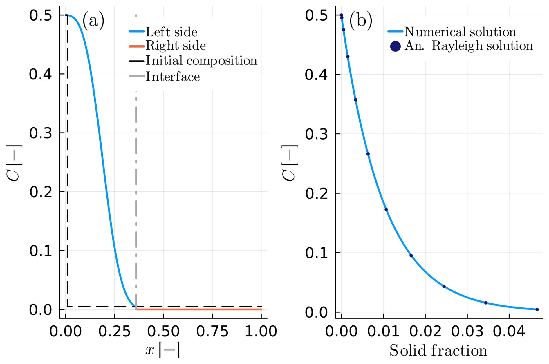
Figure C1 Example C1: as in Fig. 6 (example B4) but calculated using the total mass balance constraint (Eq. 19 in the main text).

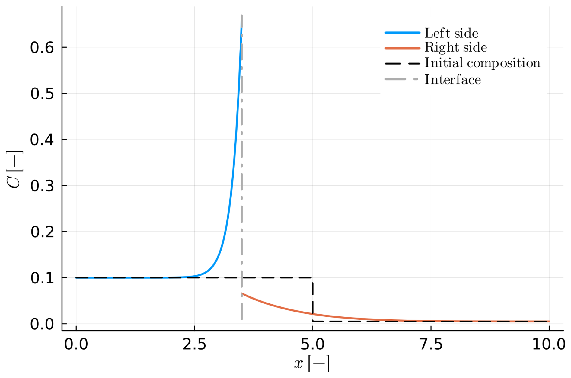
Figure C2 Example C2: same as in Fig. 9 (example B7). The mass balance at the interface was calculated using the total mass balance (Eq. 19 in the main text).