DalROMS-NWA12 v1.0, a coupled circulation–ice–biogeochemistry modelling system for the northwest Atlantic Ocean: development and validation

This study presents DalROMS-NWA12 v1.0, a coupled ocean circulation–sea ice–biogeochemistry modelling system for the northwest Atlantic Ocean (NWA) in which the circulation and biogeochemistry modules are based on ROMS (Regional Ocean Modeling System). The circulation module is coupled to a sea ice module based on the Community Ice CodE (CICE), and the physical ocean state simulated by the circulation module drives the biogeochemical module. Study of the biological carbon pump in the NWA is one of the main intended applications of this model. Global atmospheric and ocean reanalyses are used to force DalROMS-NWA12 at the sea surface and as part of its lateral boundary input, respectively. The modelling system is also forced by tides, riverine freshwater input, and continental runoff. The physical ocean state and sea ice from two simulations of the period 2015–2018, with and without nudging of the simulated temperature and salinity towards a blend of observations and reanalysis, are examined in this study. Statistical comparisons between model results and observations or reanalyses show that the control (nudged) simulation outperforms the prognostic (un-nudged) simulation in reproducing the paths of the Gulf Stream and the West Greenland Current, as well as propagation of the estuarine plume in the Gulf of St. Lawrence. The prognostic simulation performs better in simulating the sea ice concentration. The biogeochemical module, which is run only in the control simulation, performs reasonably well in reproducing the observed spatiotemporal variations in oxygen, nitrate, alkalinity, and total inorganic carbon. To examine the effects of tides and sea ice on the physical fields in the study area, results of simulations from which either component is absent are compared to results of the prognostic simulation. In the absence of tides, Ungava Bay in summer experiences a simulated surface salinity that is higher by up to ∼7 psu than in the simulation with tides, as well as experiencing changes in horizontal distributions of surface temperature and sea ice. Without coupling to the sea ice module, the circulation module produces summertime sea surface temperatures that are higher by up to ∼5 °C in Baffin Bay.

1 Introduction

The northwest Atlantic Ocean (hereafter NWA) is characterized by interactions among physical and biogeochemical processes that affect the global atmosphere–ocean system. Air-to-sea flux of CO₂ per unit area is estimated to be at its largest in the world in the Atlantic Ocean north of 50° N due to factors such as strong winds in winter and high primary production in spring (Takahashi et al., 2009). The sinking of particles formed during primary production has the effect of transporting atmospheric CO₂ to the deep ocean and is referred to as the biological carbon pump (BCP; Volk and Hoffert, 1985). The BCP is influenced by various physical processes over an annual cycle. The presence of sea ice in winter, on one hand, can drive upward transport of nutrients through brine-rejection-induced vertical mixing (Jin et al., 2018) but, on the other hand, can reduce wind-induced mixing (Rainville et al., 2011) and attenuate the solar radiation (Legendre et al., 1992) by isolating the water column from the atmosphere. Seasonal changes in the mixed-layer depth is another physical process that governs the BCP. Shoaling of the layer in spring, driven by freshwater input from runoff and sea ice, promotes primary production (Wu et al., 2007, 2008; Frajka-Williams and Rhines, 2010), while deepening of the layer in winter can result in entrainment of dissolved inorganic carbon and respiratory CO₂ that had been in shallow subsurface waters (Körtzinger et al., 2008). In the Labrador Sea, deep convection in winter is thought to be an additional pathway for removal of carbon from near-surface waters (Tian et al., 2004).

Several field programs have been conducted to quantify the major processes at work in the NWA, such as the Labrador Sea Deep Convection Experiment (The Lab Sea Group, 1998), which focused on atmospheric and physical oceanographic processes, and the Atlantic Zone Monitoring Program (Pepin et al., 2005) and its off-shelf counterpart (e.g., Yashayaev and Loder, 2017), which have made regular shipboard measurements of physical and biogeochemical (BGC) fields at fixed locations. Simultaneous measurements of physical and BGC fields at moorings (e.g., Martz et al., 2009; Strutton et al., 2011) and by profiling floats (e.g., Yang et al., 2020; Wang and Fennel, 2022) have expanded the coverage of observations, which is crucial given the spatiotemporal variability in the processes that govern the BCP (Garçon et al., 2001).

Process-based numerical models can complement observations of oceanic processes by providing four-dimensional estimates of relevant fields and by enabling experiments in which the effects of key inputs are isolated or the future state of oceans under various climate scenarios is simulated (Fennel et al., 2022). Early numerical studies of the NWA using coupled ocean circulation–sea ice models focused mainly on specific processes, such as climatological sea ice conditions (Mysak et al., 1991), sea ice variabilities on the interannual (Ikeda et al., 1996) and intra-seasonal (Yao et al., 2000) timescales, and changes in sea ice and mixed-layer properties under different atmospheric conditions (Tang et al., 1999). As process-based numerical models grew in complexity, they yielded new insights, such as the role of sea ice's heat capacity in the timing of ice melt (Zhang et al., 2004). Advances in computational power have led to realistic simulations spanning a decade or more covering limited areas, such as the Canadian Arctic Archipelago and Davis Strait (Lu et al., 2014) or the Labrador and Newfoundland shelves (Ma et al., 2016). Other ocean–ice models of areas within the NWA include that of the Gulf of St. Lawrence and surrounding waters (Urrego-Blanco and Sheng, 2014; Wang et al., 2020), Hudson Bay (Saucier et al., 2004), and the Labrador Sea (Pennelly and Myers, 2020). Canadian government agencies have developed coupled ocean–ice or atmosphere–ocean–ice models to support activities such as hazard management, with domains ranging from the regional (e.g., Smith et al., 2013, for the Gulf of St. Lawrence) to basin-wide (Dupont et al., 2015; Wang et al., 2018). Other modelling studies have focused on hydrodynamics in coastal and shelf waters of the NWA, such as Han et al. (1997) for the Scotian Shelf, Wu et al. (2012) for the area between the Gulf of Maine and Baffin Bay, and Chen and He (2015) for the Mid-Atlantic Bight and the Gulf of Maine.

As for coupled physical–BGC modelling studies, three-dimensional models with high resolutions have generally focused on the shelf and slope areas of the NWA. Pei (2022) used a simple oxygen model to study seasonal changes in dissolved oxygen over the Scotian Shelf, while more complex models have been used to study the biogeochemistry and plankton dynamics of the Scotian Shelf and surrounding waters (Laurent et al., 2021; Rutherford and Fennel, 2022) and the Gulf of St. Lawrence (Le Fouest et al., 2010; Lavoie et al., 2021). Ross et al. (2023) developed a coupled physical–BGC model for the North Atlantic Ocean from the Caribbean Sea to the southern Labrador Sea, designed primarily for marine resource management.

As coupled simulations that include more processes and cover larger extents of space and time become feasible, they are expected to enhance our understanding of how the ocean functions as an integrated system, as well as of how this system might change under various scenarios of the future climate. In this study, we present and assess a coupled ocean circulation–sea ice–BGC model that was developed recently with the primary goal of studying the interactions between physical and BGC processes in the NWA, including the BCP. Advantages of this model's configuration include (a) a domain that spans the area from the Mid-Atlantic Bight to Baffin Bay, allowing for a wide range of oceanographic processes that can be examined; (b) a horizontal grid size of O(1 km) that decreases with latitude such that the first baroclinic Rossby radius of deformation (Chelton et al., 1998) is spanned by about four grid boxes everywhere; (c) the use of a terrain-following vertical coordinate system, which can produce more realistic near-bottom vertical mixing and bottom boundary layer structures than the step-wise bottom topography of z-level grids (Ezer and Mellor, 2004); (d) tides (as one of the model inputs) and sea ice (through coupling between the circulation and sea ice modules), both of which are important elements of the ocean system in this region; and (e) a BGC module, which enables the study of how processes such as the BCP are driven by the coupled ocean circulation–sea ice system. This paper provides an assessment of the coupled model's performance as well as sensitivity studies designed to elucidate the role of two physical processes, tides and sea ice. The components of the coupled model and the simulations are described in the next section. In Sect. 3, the results of two simulations, with and without nudging of the temperature and salinity towards a blend of observations and reanalysis (referred to as the control and prognostic simulations, respectively), are described and quantitatively compared to observations or reanalysis. In addition, depth vs. time plots of simulated temperature are used to qualitatively assess the model's performance in reproducing the effects of winter convection in the Labrador Sea. In Sect. 4, the roles of tides and sea ice in the physical fields of the NWA are examined by comparing the results of two additional simulations, one without tidal forcing and the other without the simulation of sea ice, to results of the prognostic simulation described in Sect. 3. A summary of our findings is presented in the concluding section.

2 Model setup and forcing

The coupled circulation–sea ice–BGC modelling system used in this study consists of three modules: an ocean circulation module based on ROMS (Regional Ocean Modeling System, version 3.9; Haidvogel et al., 2008), a sea ice module based on CICE (Community Ice CodE, version 5.1; Hunke et al., 2015), and a BGC module within ROMS based on the work of Fennel et al. (2006, 2008) with updates as described by Laurent et al. (2021). The circulation and sea ice modules are coupled using the software MCT (Model Coupling Toolkit, version 2.10; Jacob et al., 2005; Larson et al., 2005) in a manner similar to that in Kristensen et al. (2017). Yang et al. (2023) found good agreement between simulated and observed values of tides and storm surges simulated by a barotropic version of the ocean circulation module.

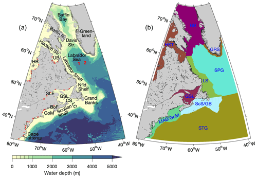
Figure 1 (a) Model domain and bathymetry. Locations of river mouths are indicated by red X marks. Locations for which depth profiles of simulated temperature are shown in Fig. 16 are indicated by numbers in red. Abbreviations are used as follows: Island (Is.), Strait (Str.), Hudson Bay (HB), Ungava Bay (UB), Newfoundland (Nfld.), St. Lawrence Estuary (SLE), Gulf of St. Lawrence (GSL), Cabot Strait (CS), Laurentian Channel (LC), Bay of Fundy (BoF), and Gulf of Maine (GoM). (b) Regions in which metrics of model performance are calculated. The regions are as follows: GRS (Greenland Shelf), HST (Hudson Strait), BB (Baffin Bay), LS (Labrador Shelf), SPG (North Atlantic Subpolar Gyre), GSL (Gulf of St. Lawrence), ScS/GB (Scotian Shelf and Grand Banks), MAB/GoM (Mid-Atlantic Bight and Gulf of Maine), and STG (North Atlantic Subtropical Gyre). Areas within 10 grid points of lateral boundaries are excluded from the error metric calculations.

ROMS is a three-dimensional (3D) numerical circulation model with a free surface and the terrain-following S-coordinate system (originally developed by Song and Haidvogel, 1994) in the vertical. The vertical layers are placed more densely near the surface and bottom in deep waters and more uniformly in shallow waters. In this study ROMS has 40 vertical S layers, whose configuration is described in Appendix A. ROMS and CICE use the same horizontal grid and bathymetry, with the domain covering the area between ∼81 and ∼39° W and between ∼33.5 and ∼76° N (Fig. 1a). The grid resolution in the east–west direction is $\mathrm{1}/\mathrm{12}$°, resulting in grid box dimensions of ∼8 km on each side near the grid's southern boundary and ∼2 km on each side near the northern boundary.

The model bathymetry is derived from the $\mathrm{1}/\mathrm{240}$° resolution data set GEBCO_2019 (GEBCO Compilation Group, 2019). After the GEBCO data were linearly interpolated onto the model grid, the Shapiro filter (Shapiro, 1975) was applied to seamounts in deep waters from ∼67.5 to ∼42° W and from ∼34 to ∼48° N to reduce currents caused by spurious pressure gradients. No other smoothing was applied to the bathymetry. To avoid model instability caused by strong currents entering the model domain at an angle, the model bathymetry and land–sea mask in the first four grid boxes from each lateral boundary were set to the same values as in the fifth grid box from the boundary.

The advection schemes used in ROMS for physical fields are (a) the third-order upstream scheme for horizontal advection of physical tracers and 3D momentum and (b) the fourth-order centred scheme for horizontal advection of two-dimensional momentum and for vertical advection of physical tracers and 3D momentum. The horizontal eddy viscosity and diffusivity in ROMS are set to zero because the third-order upstream scheme generates some numerical diffusion which is large enough to eliminate small-scale features associated with numerical noise. Vertical mixing is parameterized using the “2.5-level” scheme of Mellor and Yamada (1982) with modifications as described by Allen et al. (1995). The time step is 6 s for the external (barotropic) mode and 120 s for the internal (baroclinic) mode.

Atmospheric fields used to drive the coupled model are derived from the hourly reanalysis data set known as ECMWF Reanalysis v5 (ERA5; Hersbach et al., 2018), which has horizontal grid spacing of $\mathrm{1}/\mathrm{4}$°. Within ROMS, the bulk flux scheme of Fairall et al. (1996a, b) is used to calculate the surface fluxes of heat and fresh water. Lateral open boundary conditions are specified using the explicit scheme of Chapman (1985) for sea surface elevation, the Shchepetkin scheme (Mason et al., 2010) for the normal component and the implicit scheme of Chapman (1985) for the tangential component of depth-averaged currents, and the adaptive scheme of Marchesiello et al. (2001) for the normal and tangential components of depth-varying currents as well as all tracers. In the adaptive boundary condition, the nudging timescale is 3 d for inflow and 360 d for outflow. The values of currents, temperature, salinity, and sea surface elevation specified at the lateral boundaries are derived from the daily fields of Copernicus global $\mathrm{1}/\mathrm{12}$° oceanic and sea ice reanalysis (GLORYS12V1, hereafter GLORYS; Lellouche et al., 2021) for the simulation period. In order to ensure that the simulated ocean states near lateral open boundaries are as realistic as possible, the lateral boundary conditions of currents, temperature, and salinity are supplemented by nudging the simulated values near boundaries towards GLORYS values. The nudging timescale is 3 d at the grid point closest to a lateral boundary and decreases linearly to zero over 10 grid points moving away from the boundary. Tidal elevation and currents are specified at the lateral boundaries from the global tidal model solution TPXO9v2a (an updated version of the model by Egbert and Erofeeva, 2002), with a horizontal grid size of $\mathrm{1}/\mathrm{6}$° and 15 tidal constituents.

Table 1 Names and discharge locations of rivers in the coupled model.

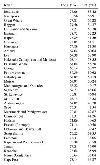
Riverine freshwater input from 35 rivers (Table 1) is specified as volume flux through the bottom of a model grid cell (http://www.myroms.org/forum/viewtopic.php?t=5156, last access: 26 November 2024). Each river is represented by a channel normal to the model's coastline, at the head of which the surface elevation, vertical velocity, and tracer values are adjusted according to the river discharge. The river water has a salinity of 0.4 psu (salinity in the Practical Salinity Scale is dimensionless, but we use the unit “psu” for clarity) and a temperature equal to that of the GLORYS sea surface temperature at the grid point closest to the river mouth. For the St. Lawrence River, we use the monthly-mean discharge at the city of Québec estimated by the St. Lawrence Global Observatory (2023) using the regression model of Bourgault and Koutitonsky (1999). For all other rivers, we use the monthly-mean data set of Dai (2017) that was updated in May 2019, substituting climatological values calculated over the period 1900–2018 for months with no data. Freshwater flux across coastlines due to the melting of ice and snow over land is specified as an addition to the sea surface height and the surface freshwater flux at the appropriate model grid boxes. This freshwater flux is derived from the monthly data set of Bamber et al. (2018), who combined satellite observations of glaciers with the output of a regional climate model. A monthly climatology of this data set, which covers the period 1958–2016, is used in simulations of the period after December 2016. Both the riverine and the continental freshwater fluxes are converted to “pseudo-means” (monthly means that are adjusted such that daily-mean values temporally interpolated from them, when summed over a month, result in the true monthly means) following Killworth (1996). Another source of salt/freshwater flux at the sea surface is sea ice, which is a source of salt through brine rejection at the time of freezing and a source of fresh water at the time of melting. Lateral movement of sea ice results in these two surface fluxes occurring at different locations.

The sea ice model CICE consists of four main components: (a) a thermodynamic component that calculates local growth or decay of sea ice due to snowfall and heat fluxes (Bitz and Lipscomb, 1999; Briegleb and Light, 2007), (b) a dynamic component that calculates the material properties of the ice (Hunke and Dukowicz, 1997; Bouillon et al., 2013), (c) a transport component that calculates the horizontal advection of the ice (Lipscomb and Hunke, 2004), and (d) a component that calculates the distribution of ice among thickness categories due to ridging and mechanical processes (Hunke et al., 2015). There are seven ice layers and five ice thickness categories. We implemented the clamped boundary condition, in which GLORYS-derived values of sea ice concentration (as a fraction of the model grid box area) and thickness are specified at the model's lateral open boundaries. The sea ice specified at the lateral boundaries is uniformly covered with snow of 0.2 m thickness. The time step in CICE is 1200 s.

Coupling between ROMS and CICE via MCT occurs every 1200 s, equivalent to every 10 internal time steps in ROMS and every time step in CICE. At each coupling step, ROMS sends CICE the ERA5-derived atmospheric fields that drive both modules, as well as ROMS-simulated values of currents, sea surface tilt, and sea surface values of temperature and salinity. CICE sends ROMS the ice-attenuated value of shortwave radiation and ice–ocean fluxes of stress, heat, and salt or fresh water.

The BGC module includes the nitrogen cycle (Fennel et al., 2006), the carbonate system (Fennel et al., 2008), and oxygen (Fennel et al., 2013). Particulate organic matter variables (phytoplankton, zooplankton, and detritus) are split into small and large size classes, and rates of biological processes are temperature-dependent (Laurent et al., 2021). The HSIMT advection scheme (Wu and Zhu, 2010), which ensures no spurious negative values occur, is used for both horizontal and vertical advection of BGC tracers. Initial and boundary conditions for nitrate, phosphate, dissolved inorganic carbon, alkalinity, and oxygen are interpolated from the climatology of GLODAP (Global Ocean Data Analysis Project; Lauvset et al., 2021) and are set to small constant values for all other biogeochemical variables.

Four simulations will be examined in this paper. In the control simulation (hereafter Ctrl), the ocean temperature and salinity at all grid points are nudged with a restoring timescale of 60 d towards the monthly data set of in situ observations known as CORA (Coriolis Ocean database for ReAnalysis; Cabanes et al., 2013) above 2000 m depth and towards GLORYS below 2000 m (where CORA data are not available). The control simulation includes biogeochemistry. The second simulation is a prognostic one (hereafter Prog), i.e., without any nudging of the simulation. There are three reasons for presenting these simulations: (1) the ways in which either simulation outperforms the other can shed light on potential ways in which the model can be improved; (2) Ctrl, by including nudging of the temperature and salinity, produces a physical state of the ocean that is generally realistic and acts as a foundation for the biogeochemical simulation; and (3) this modelling system is being used in regional climate simulations, and the lack of an option to nudge simulations of future conditions necessitates assessment of a prognostic simulation. The performance of Ctrl and Prog will be evaluated in the next section. Two more simulations are carried out for the sensitivity studies discussed in Sect. 4. Both are identical to Prog, but one is made without the specification of tidal elevation and currents at the lateral boundaries (hereafter NoTides) and the other is made without coupling of ROMS to CICE (hereafter NoIce). Configurations of the simulations are summarized in Table 2. All simulations are made from 1 September 2013 to 31 December 2018 and are initialized with an ice-free ocean in which the ocean's state consists of GLORYS fields for 1 September 2013 interpolated to the model grid. The simulation results of January 2015 onwards (December 2014 onwards in the case of seasonal averages) will be discussed in the following sections.

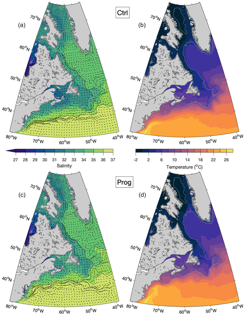
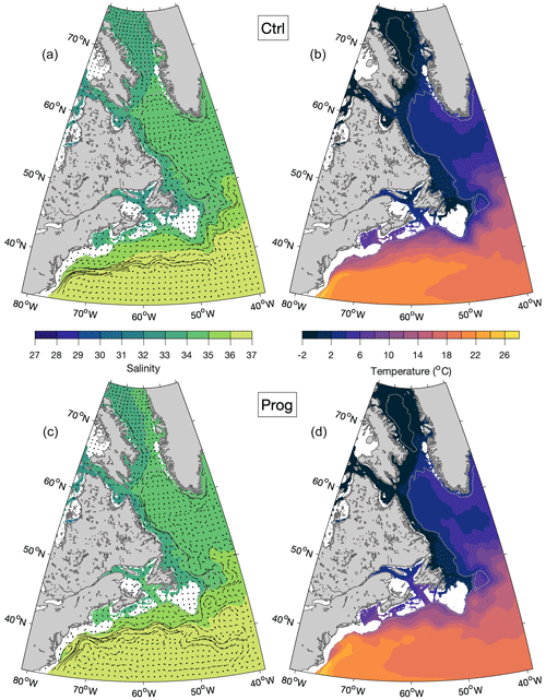
Figure 2 Temporal-mean salinity (a, c) and temperature (b, d) at the sea surface, averaged over 2015–2018, from the Ctrl (a, b) and Prog (c, d) runs. Also shown in panels (a) and (c) are trajectories representing displacement over 5 d due to currents at the sea surface averaged over 2015–2018, shown at every 24th model grid point. The grey contour line represents the 1000 m water depth.

Figure 3 Similar to Fig. 2 but for model results interpolated to the 100 m depth.

Table 2 Descriptions of the simulations discussed in this study.

3 Model results and evaluation

3.1 Simulated currents, temperature, and salinity

We first examine 4-year (1 January 2015–31 December 2018) averages of currents, salinity, and temperature produced by DalROMS-NWA12 v1.0 in the Ctrl and Prog runs (Figs. 2 and 3, respectively). Both model runs reproduce the major features of the circulation in this region. They include (a) the East Greenland and West Greenland currents forming a clockwise flow around the southern tip of Greenland; (b) bifurcation of the West Greenland Current, with one branch continuing northwards along the west coast of Greenland and the other flowing westwards across the Labrador Sea; and (c) the westward flow across the Labrador Sea merging with the southward Baffin Island Current out of Baffin Bay and southeastward flow out of the Hudson Strait to form the Labrador Current, the equatorward limb of the North Atlantic Subpolar Gyre. This current has branches along the Labrador coast and the shelf break. Near the Grand Banks, the Labrador Current meets the poleward Gulf Stream, the poleward limb of the North Atlantic Subtropical Gyre. Both simulations also reproduce the relatively cold and fresh water over continental shelves, with especially low values of salinity in Hudson Bay and the St. Lawrence Estuary. The three major differences between the simulations are that (a) the bifurcation of the West Greenland Current has a stronger northward branch in Prog; (b) the Gulf Stream in Prog is closer to the continental shelf; and (c) the Gulf of St. Lawrence is warmer and saltier in Prog, both at the surface and in model results interpolated to a 100 m depth. As discussed below, comparison of model results to observations or reanalysis suggests the results of Ctrl are more realistic than those of Prog. Seasonal means of these simulated fields, shown in Appendix B, indicate that differences between the simulations are more prominent in summer than in winter.

3.2 Model performance for currents, temperature, and salinity

To assess the model's performance in simulating currents, temperature, and salinity, we divide the model domain into nine regions (Fig. 1b) and calculate metrics in each region for model results at the sea surface and interpolated to the 100 m depth. Within a given region, each model grid point is weighted by its horizontal area when regional averages are calculated. The areas along the model's lateral boundaries in which the simulated tracers and currents are nudged towards GLORYS are not included in the calculations.

To quantify model performance for temperature and salinity at the sea surface, root-mean-square errors (RMSEs) of monthly-mean model results are calculated with respect to monthly means of observations that are linearly interpolated to the model grid. Temperature and salinity at the surface are compared to analyzed $\mathrm{1}/\mathrm{4}$° grid data sets that combine satellite and in situ observations: the daily data set OISST (Optimum Interpolation Sea Surface Temperature, v2.0 for 2015–2017 and v2.1 for 2018; Huang et al., 2021) for temperature and the weekly data set SMOS (Soil Moisture Ocean Salinity; Buongiorno Nardelli et al., 2016) for salinity. For model results interpolated to the 100 m depth, where gridded observational data sets are not available, root-mean-square differences (RMSDs) of temperature and salinity are calculated with respect to their respective GLORYS values. It should be noted that GLORYS is based on simulations that do not include tides (Lellouche et al., 2018), which may affect the accuracy of its temperature and salinity distributions in addition to the distributions of its currents, particularly over areas with strong tidal currents. It should also be noted that the oceanographic observations used in generating GLORYS are highly sparse in both time and space. As a result, data assimilation cannot completely eliminate biases associated with the exclusion of tidal forcing in the monthly-mean fields of GLORYS.

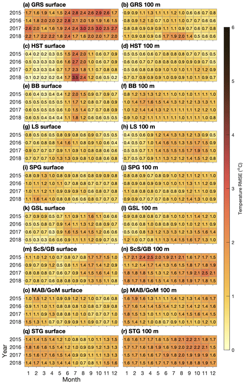
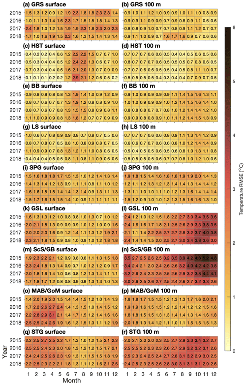
Figure 4 Root-mean-square errors/differences in temperatures simulated in Ctrl, calculated for the regions shown in Fig. 1b with respect to the observation-derived OISST data set at the surface and GLORYS reanalysis for model results interpolated to the 100 m depth.

Figure 5 Similar to Fig. 4 but for temperatures simulated in Prog.

The RMSE and RMSD of temperature from the two simulations (Figs. 4–5) are similar over the northern part of the model domain in that the largest errors tend to occur at the surface in GRS (Greenland Shelf) throughout the year and in HST (Hudson Strait) and BB (Baffin Bay) during the summer. Within these three areas, the largest values of RMSE and RMSD occur in HST at the surface (about 3.5 °C in Ctrl and 2.9 °C in Prog, both in July). The corresponding biases of surface temperatures (not shown) indicate a tendency towards overestimation (+0.3 to +2.2 °C in GRS and −0.4 to +1.9 and −0.5 to +1.0 °C during summer in HST and BB, respectively, for Prog). Thus, the largest errors occur near the model's lateral open boundaries, during periods when sea ice (which would tend to keep the temperature near freezing) is reduced in HST and BB, and at the surface where the performance metrics are calculated with respect to an independent observational data set instead of GLORYS, which is also used as lateral boundary input. This suggests GLORYS as a possible source of model errors, although a detailed examination is beyond the scope of this study. The slightly larger RMSE of the simulated surface temperature in Ctrl compared to Prog over these areas may be related to the larger underestimation of sea ice in Ctrl, which will be discussed in Sect. 3.3.

Further south, in SPG (North Atlantic Subpolar Gyre), the RMSE and RMSD are smaller in Ctrl than in Prog. The RMSE at the surface has a range of 0.6–1.6 °C in Ctrl and 0.9–2.1 °C in Prog, and the RMSD for model results interpolated to the 100 m depth has a range of 0.7–1.4 °C in Ctrl and 0.9–2.0 °C in Prog. This suggests the West Greenland Current simulated in Ctrl, in which the branch of the current that separates from the Greenland coast dominates, and its associated temperature distribution are more realistic. The RMSE and RMSD for LS (Labrador Shelf) are similar between the simulations, ranging from 0.4 to 1.9 °C in Ctrl and from 0.4 to 1.4 °C in Prog.

The results of Ctrl clearly outperform those of Prog over the southern part of the model domain, with a maximum RMSE and RMSD of ∼2.5 °C in the former and ∼5.2 °C in the latter, both occurring at ScS/GB (Scotian Shelf and Grand Banks) for model results interpolated to the 100 m depth. This indicates that the Gulf Stream simulated in Ctrl, flowing further from the coast than in Prog (Figs. 2–3), is more realistic. In addition to STG (North Atlantic Subtropical Gyre) where the Gulf Stream itself flows, the RMSE and RMSD in Ctrl are smaller at both the surface and the 100 m depth in ScS/GB, MAB/GoM (Mid-Atlantic Bight and Gulf of Maine), and GSL (Gulf of St. Lawrence), all of which are influenced by the warm and salty slope water of which the Gulf Stream water is one component (Gatien, 1976). The influence of the slope water extending into the GSL at the 100 m depth (which can also be seen in Fig. 3) is consistent with the observed (e.g., Richaud et al., 2016) intrusion of slope water into the Gulf of St. Lawrence along the Laurentian Channel.

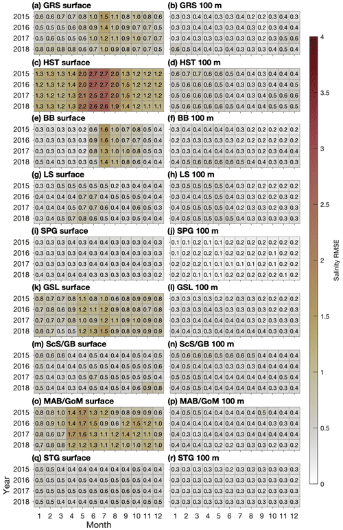
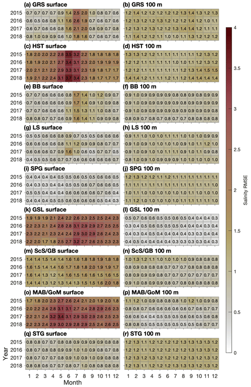
Figure 6 Root-mean-square errors/differences in salinity simulated in Ctrl, calculated for the regions shown in Fig. 1b with respect to the observation-derived SMOS data set at the surface and GLORYS reanalysis for model results interpolated to the 100 m depth.

Figure 7 Similar to Fig. 6 but for salinity simulated in Prog.

The RMSE and RMSD of salinity for both simulations (Figs. 6–7) in the northern part of the model domain are similar to those of temperature in that they tend to be largest at the surface in summer, especially in HST where the RMSE has maximum values of ∼2.7 psu in Ctrl and ∼3.7 psu in Prog. In contrast to the temperature metrics, the surface salinity metrics in GRS undergo an annual cycle similar to those in HST and BB, being larger during summer and fall than during the rest of the year. During the months when the RMSEs are largest, the surface salinity biases for Prog are negative in GRS and BB (ca. −1.0 psu) and positive in HST (up to ca. +1.5 psu). In SPG and LS the RMSE and RMSD are generally smaller in Ctrl than in Prog (0.1–0.8 psu for Ctrl and 0.4–1.5 psu in Prog for the two regions combined), which is consistent with the metrics for temperatures discussed above.

In the southern part of the domain, Ctrl has much smaller RMSE than Prog in GSL, ScS/GB, and MAB/GoM (e.g., the maximum value is ∼1.7 psu for Ctrl and ∼3.7 psu for Prog in MAB/GoM). The corresponding biases for Prog in these areas are consistently positive (up to ca. +3.3 psu in GSL), indicating overestimation. However, within GSL, the 2015–2018 mean of summer surface salinity simulated by Prog is lower than its counterpart simulated by Ctrl by up to ∼3.5 psu in the St. Lawrence Estuary but higher by ∼2.0 psu further downstream in the Gulf of St. Lawrence (not shown). This suggests that the model is not able to fully reproduce the propagation of low-salinity water from the St. Lawrence Estuary (where the salinity is underestimated) to areas downstream of it (where the salinity is overestimated).

A possible cause of this discrepancy between observed and simulated salinity values in the St. Lawrence Estuary–Gulf of St. Lawrence system is spurious diapycnal mixing generated by the third-order upstream advection scheme used for tracers in this study (Marchesiello et al., 2009). We found that switching to the fourth-order Akima scheme (with a horizontal eddy diffusivity of 5 m² s⁻¹) leads to more realistic simulations of three-dimensional salinity distributions and sea ice distributions in the gulf, but this option was not pursued further because the scheme is prone to over- or under-shooting, which resulted in patches of unrealistic tracer values in areas such as the Grand Banks where strong horizontal gradients occur. The same problem was reported by Naughten et al. (2017) in simulating circulation in the Southern Ocean using ROMS and CICE. A potential solution is a fourth-order advection scheme with a flux limiter to eliminate the spurious over- and under-shooting, as demonstrated by Sheng (2002) for a z-level ocean model.

For currents, the model performance is evaluated using a metric known as ε² (Schwab et al., 1989; Urrego-Blanco and Sheng, 2014):

$$\begin{array}{}\text{(1)}& {\mathit{\epsilon }}^{\mathrm{2}}={\displaystyle \frac{{\sum }_{i=\mathrm{1}}^N\left[{\left(U_i^{\mathrm{O}}-{\overline{U}}_i^{\mathrm{O}}-U_i^{\mathrm{M}}+{\overline{U}}_i^{\mathrm{M}}\right)}^{\mathrm{2}}+{\left(V_i^{\mathrm{O}}-{\overline{V}}_i^{\mathrm{O}}-V_i^{\mathrm{M}}+{\overline{V}}_i^{\mathrm{M}}\right)}^{\mathrm{2}}\right]}{{\sum }_{i=\mathrm{1}}^N\left[{\left(U_i^{\mathrm{O}}-{\overline{U}}_i^{\mathrm{O}}\right)}^{\mathrm{2}}+{\left(V_i^{\mathrm{O}}-{\overline{V}}_i^{\mathrm{O}}\right)}^{\mathrm{2}}\right]}},\end{array}$$

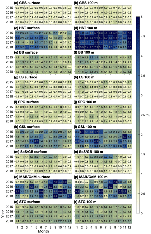
where the superscripts “O” and “M” denote observed and simulated values, respectively; overbars denote spatial averaging over each validation region; and the summation is made over the validation region. Thus, this metric combines errors for the zonal and meridional current components and assesses model performance in terms of spatial averages as well as at individual points, with a value of zero corresponding to perfect agreement between model results and observations. The metric is calculated with respect to GLORYS both at the surface and for model results interpolated to the 100 m depth.

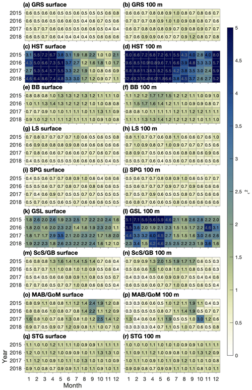
Figure 8 ε² of currents simulated in Ctrl, calculated for the regions shown in Fig. 1b with respect to GLORYS reanalysis. See Eq. (1) for the definition of ε².

Figure 9 Similar to Fig. 8 but for currents simulated in Prog.

For both simulations, values of ε² (Figs. 8–9) in the southern part of the model domain are generally smaller in Ctrl than in Prog (e.g., about 0.7–1.3 for Ctrl vs. 1.0–2.2 for Prog in STG), consistent with the more realistic simulation of the Gulf Stream due to the nudging of salinity and temperature in Ctrl. In SPG and LS, values of ε² are similar between the regions and smaller in Ctrl than in Prog (about 0.4–1.1 in Ctrl and 0.5–1.6 in Prog for the two regions combined). This suggests that the Labrador Current is more realistic in Ctrl than in Prog, which is consistent with the conclusion drawn from the temperature metrics that the separation of the West Greenland Current from the Greenland coast is simulated more accurately in Ctrl.

The model errors for both runs are largest in HST, mostly due to the southeastward flow along the south side of the Hudson Strait being stronger in the model than in GLORYS (not shown). Taking as an example the 2015–2018 mean of monthly-mean currents produced by Prog in September, the southeastward flow is stronger than that in GLORYS by ∼0.25 m s⁻¹ at the surface and ∼0.15 m s⁻¹ at the 100 m depth. One possible reason for this large discrepancy is that the model is likely to be unable to accurately simulate the circulation in Hudson Bay, which is the source of the southeastward flow through the Hudson Strait. Circulation in the bay consists of several gyres and is sensitive to river discharge (Ridenour et al., 2019). Our model domain includes only the eastern part of the bay (Fig. 1a), and, due to a lack of observations, we use climatological discharge (mostly calculated from observations in the 1960s or 1970s) for all but 1 of the 10 rivers emptying into the eastern bay; these factors cast doubt on the model's ability to realistically simulate the flow within and out of the bay.

It should also be noted that the Hudson Strait is characterized by tides of typically 3–6 m in amplitude (Drinkwater, 1988). While our model includes tidal forcing, GLORYS, as stated above, does not. This raises questions about how appropriate GLORYS is as a basis of evaluating simulated currents in this area. Drinkwater (1988) deployed an array of current meters across the Hudson Strait between August and October in 1982. While exact coordinates of this array are not available, the grid point in our model closest to the southwestern end of the array (station HS1) can be approximated as 61.15° N, 69.47° W, with a water depth of 272 m, from Figs. 1–2 of Drinkwater (1988). The 8-week average of residual current speeds at this location was observed to be about 0.29 and 0.12 m s⁻¹ at the 30 and 100 m depths, respectively. The 2015–2018 averages of September mean current speeds simulated by Prog and from GLORYS at the corresponding model grid point are similar to each other and somewhat lower than the observed value at the 30 m depth (about 0.24 and 0.23 m s⁻¹, respectively, vs. 0.29 m s⁻¹). However, at the 100 m depth, the simulated mean current speed (0.10 m s⁻¹) is more similar to the observation (0.12 m s⁻¹) than the GLORYS value (0.03 m s⁻¹). Although we need to keep in mind the existence of interannual variability and long-term trends which limit the conclusions we can derive, these comparisons point to the possibility that the inclusion of tides in our model may result in a more realistic vertical structure of currents in areas where both tides and baroclinicity play significant roles. The role of tides in the NWA is explored further in Sect. 4.1.

The temperature and salinity simulated in Prog have also been compared to observations made along transects from the Atlantic Zone Monitoring Program and its off-shelf counterpart (not shown). RMSEs along the AR7W transect, which spans the Labrador Sea between southern Labrador and southern Greenland, are largest near the surface, reaching ∼2 °C for temperature and ∼0.5 for salinity. The errors are larger in transects across the Cabot Strait and across the Scotian Shelf (up to ∼4 °C for temperature and ∼3 for salinity), reflecting the difficulty Prog has in reproducing the estuarine circulation in the Gulf of St. Lawrence and the positions of the Gulf Stream and slope waters.

The preceding description and evaluation of the simulated circulation and hydrography have highlighted two features in which the nudging of temperature and salinity in Ctrl leads to improved model performance: (a) the separation of currents (the Gulf Stream and West Greenland Current) from their respective coasts and (b) propagation of the low-salinity plume from the St. Lawrence Estuary. Chassignet and Xu (2017) and Pennelly and Myers (2020) showed that increasing the horizontal resolution of their model grids from $\mathrm{1}/\mathrm{12}$ to $\mathrm{1}/\mathrm{50}$ and to $\mathrm{1}/\mathrm{60}$°, respectively, resulted in more realistic representations of the Gulf Stream and the West Greenland Current. Given the computational costs of making coupled physical–biogeochemical simulations with a finer horizontal grid than what we currently use, a possible way to improve our modelling system's performance in prognostic simulations would be to nest a finer-resolution grid covering an area of particular interest (e.g., the Labrador Sea) within the existing $\mathrm{1}/\mathrm{12}$° grid. As discussed earlier, a fourth-order horizontal advection scheme with a flux limiter is a possible way to improve our model's simulation of estuarine plumes in prognostic simulations.

Figure 10 Monthly-mean simulated sea ice concentration (a, c) and effective sea ice thickness (sea ice cover multiplied by thickness) (b, d) for February, averaged over 2015–2018, from Ctrl (a, b) and Prog (c, d). The grey contour line represents the 1000 m water depth.

3.3 Sea ice

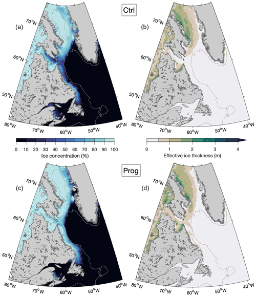
February mean values of sea ice cover and effective sea ice thickness (sea ice cover multiplied by thickness), averaged over 2015–2018, are shown in Fig. 10. Model results from Ctrl and Prog are similar in that the ice cover spans the Hudson Strait and adjoining areas to its west as well as most of Baffin Bay and the thickest ice (thickness ≳3.0 m) occurs along the coasts of those areas. The two runs are different in that Ctrl produces more ice along the west coast of Greenland and in the northwest Gulf of St. Lawrence, while Prog produces more ice along the north side of the Hudson Strait and on the Labrador Shelf. The larger sea ice production by Ctrl for the west coast of Greenland and the northwest GSL is consistent with the lower sea surface salinity and temperature in this simulation due to the nudging (Fig. 2). For the northern Hudson Strait and the Labrador Shelf, a possible factor in the larger sea ice production by Prog is the fact that, in these areas, offshore winds tend to cause ice divergence, which in turn leads to new ice formation (Babb et al., 2021; Prinsenberg and Peterson, 1992). The cycle of open-water formation, freezing, and ice divergence implies changes in the surface temperature and salinity over relatively small spatiotemporal scales, which could be dampened by the nudging of Ctrl to the monthly CORA data set with a horizontal resolution of 0.2–0.5° in our study area (Szekely, 2023). The role of sea ice in the physical oceanography of our study area is studied further in Sect. 4.2.

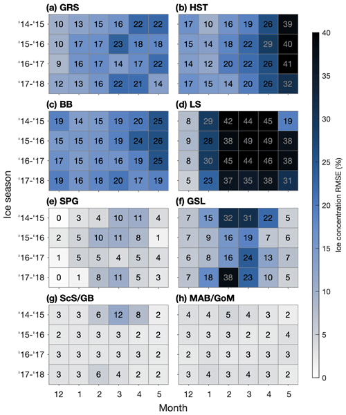
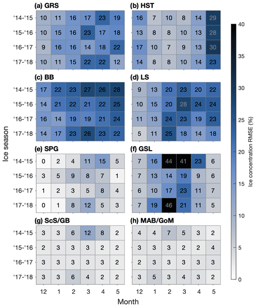
Figure 11 Root-mean-square errors in ice concentration simulated in Ctrl, calculated for the regions shown in Fig. 1b with respect to AMSR2 satellite observations.

Figure 12 Similar to Fig. 11 but for ice concentration simulated in Prog.

The ice model's performance is evaluated in terms of RMSE with respect to daily AMSR2 (Advanced Microwave Scanning Radiometer 2) observations, available on a 6.5 km grid (Melsheimer and Spreen, 2019). The model errors in HST, BB, and LS are generally larger in Ctrl (Fig. 11) than in Prog (Fig. 12), consistent with the smaller sea ice production in these areas by the former. In HST, the increase in model error during May for both runs is mostly due to underestimation, indicating melting of the ice that is too early. Given that this seasonal increase in model error occurs in both runs, the cause of the underestimation may be related to ice advection instead of thermodynamics. Examination of sea ice budgets for areas within the NWA is a possible topic of future studies.

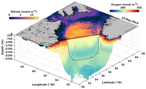
Figure 13 Three-dimensional view of simulated surface nitrate and subsurface oxygen for 15 May 2015. The thick black line at the sea surface denotes the position of the AR7W transect, and the thin black line represents the model's bottom topography along the transect.

Figure 14 Comparison of simulated (background) versus observed (dots) for oxygen (a), nitrate (b), alkalinity (c), and total inorganic carbon (d) during the AR7W transect in May 2015. Note that the y axis has higher resolution in the upper 200 m.

3.4 Biogeochemistry

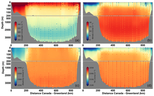
Snapshots of surface nitrate and subsurface oxygen in the Labrador Sea and surrounding areas at the time of the Atlantic Zone Off-Shelf Monitoring Program (AZOMP) cruise in May 2015 are shown in Fig. 13. The simulation indicates that nitrate starts to be depleted in the northern Labrador Sea and along the Labrador Shelf at this time but remains high in the deep central Labrador Sea. Surface and shelf waters are well oxygenated, and subsurface conditions along the AR7W transect are characteristic of the water masses – oxygenated Labrador Sea Water (depth <2000 m), lower-oxygen Northeast Atlantic Deep Water (2000–3000 m), and the more oxygenated Denmark Strait Overflow Water (>3000 m) – which is in line with the observations along the AR7W transect (Fig. 14a). Simulated nitrate is also characteristic of the three water masses (Fig. 14b). As is also shown in Fig. 13, surface nitrate remains high in the central Labrador Sea but is low or depleted on the West Greenland and Labrador shelves. These patterns agree with the observations. The spatial variability in alkalinity (Fig. 14c) and total inorganic carbon (TIC; Fig. 14d) along the AR7W transect is also well represented. The largest mismatch occurs for TIC, which is underestimated in the subsurface layers (depths >200 m).

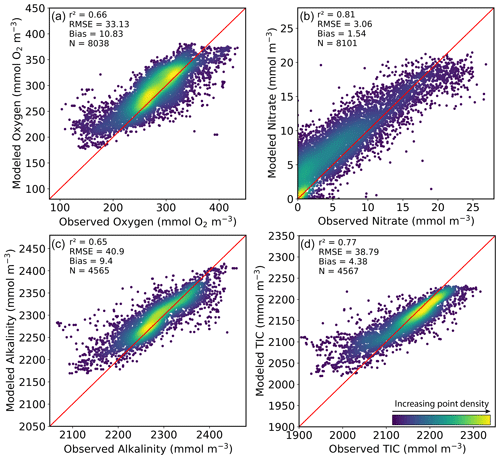
Figure 15 Comparison between simulated values and AZMP–AZOMP bottle observations during 2014–2018 for oxygen (a), nitrate (b), alkalinity (c), and total inorganic carbon (d). N is the number of observations used for the comparison.

Comparison of simulated oxygen, nitrate, alkalinity, and TIC to AZMP and AZOMP in situ observations, at locations ranging from the Gulf of Maine to the Labrador Shelf, was carried out for the period 2014–2018 (Fig. 15). The model simulates the spatial and temporal variability in biogeochemical variables reasonably well ($\mathrm{0.65}<r^{\mathrm{2}}<\mathrm{0.81}$). Simulated oxygen has a small positive bias (10.8 mmol m⁻³, Fig. 15a) but otherwise agrees with observations. Nitrate has the best match with observations (r²=0.81) but with a small positive bias (Fig. 15b), possibly driven by excess vertical mixing or by a delay in the seasonal uptake. The small bias at low TIC (i.e., surface) is likely to have the same source (Fig. 15d).

3.5 Simulation of deep convection in the Labrador Sea

One of the important hydrodynamic features of the NWA is the occurrence of deep winter convection (DWC) in the Labrador Sea and a few other areas. DWC ventilates the deep ocean, contributes to the removal of anthropogenic carbon from near-surface waters, and is thought to influence the larger-scale Atlantic Meridional Overturning Circulation (e.g., Rhein et al., 2017). In this section, we assess the model performance in reproducing the effects of DWC at two locations (indicated by numbers in Fig. 1): location 1 (58.29° N, 54.31° W) which is near the centre of the “convective region” identified by Luo et al. (2014), and location 2 (58.29° N, 50.72° W), which is on the AR7W transect and is within the area (“Central Labrador Sea”) for which Yashayaev (2024, hereafter Y24) composited the available observations to form time series of ocean properties from the surface to the 2000 m depth. (Location 1 is near the western edge of the Central Labrador Sea as defined by Y24.) The output of Prog will be used here so that the model's response to the conditions that trigger DWC can be assessed. Because the time series of Y24 indicated that conditions in 2014 were markedly different from those of subsequent years, the model results of 2014 will be included here even though they were excluded from the preceding discussions of model performance.

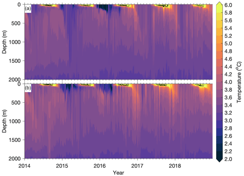
Figure 16 Daily-mean simulated temperatures from Prog, vertically interpolated to 5 m depth intervals between the 0 and 2000 m depths, at location 1 (58.29° N, 54.31° W) (a) and location 2 (58.29° N, 50.72° W) (b), indicated as “1” and “2”, respectively, in Fig. 1. Major tick marks correspond to 1 January of each year, and minor tick marks correspond to the first days of February–December. Temperature values between 6 and 11 °C are shown with black contour lines at 1 °C intervals.

Time series of temperature profiles at the two locations are shown in Fig. 16. The time series at location 1 is generally more similar to the observation-based, area-composite time series of Y24 (Y24's Fig. 3) than that of location 2. This is consistent with the fact that location 1 is at the centre of the area where DWC occurred in the modelling study of Luo et al. (2014), which the authors found to agree with areas of convection observed by, for example, Lavender et al. (2000). The time series of simulated temperature profiles at location 1 includes several features that appear in Y24, such as (1) the turbulent vertical mixing or convection being much stronger in 2015 than in 2014, with the 3.4 °C contour of simulated temperatures extending down to the ∼1600 m depth in 2015 but just to the ∼1000 m depth in 2014; (2) temperatures below 3 °C occurring from the surface to the ∼200 m depth from late 2015 to early 2016; and (3) temperatures above 6 °C extending to a maximum of ∼100 m below the surface during the summer. Given that (1) our model does not directly simulate or parameterize deep convection and (2) we are comparing the temporal evolution of simulated temperatures at one location against a composite of observations over an area with a diameter of O(100 km) in Y24, we find these similarities encouraging.

It should be noted that the horizontal grid size of our model is O(1 km), which is much coarser than the typical horizontal scale of O(100 m) for the convective plumes (e.g., The Lab Sea Group, 1998). Furthermore, our circulation model does not use an explicit DWC scheme; instead it uses large vertical mixing coefficients produced by the modified 2.5-level scheme of Mellor and Yamada (1982) to mimic the intense convective mixing associated with DWC. A fine-resolution model with a horizontal grid size of O(100 m) nested within DalROMS-NWA12 v1.0 will be used in our future research to develop better parameterizations of DWC over the NWA and to examine how the model simulates deep ocean ventilation and near-surface carbon removal due to DWC.

4 Sensitivity studies

The ocean circulation and sea ice modules of DalROMS-NWA12 v1.0 are used in this section to examine the roles of tides and sea ice in the hydrodynamics of the NWA. This is done by comparing the model results from Prog to those from two additional simulations that are identical to Prog but with the tidal forcing absent from one (NoTides) and sea ice absent from the other (NoIce). In NoIce, the net surface heat flux is set to zero if it would cool the ocean and the sea surface temperature is already at or below the local freezing temperature. The difference between surface temperatures simulated in Prog and in NoTides (Prog minus NoTides) will be denoted $\mathrm{\Delta }{T}_{\mathrm{sfc}}^{\mathrm{P}-\mathrm{NT}}$, and the difference in bottom temperatures will be denoted $\mathrm{\Delta }{T}_{\mathrm{btm}}^{\mathrm{P}-\mathrm{NT}}$. Similar notations will be used for differences in salinity (e.g., $\mathrm{\Delta }{S}_{\mathrm{sfc}}^{\mathrm{P}-\mathrm{NT}}$) and current speed (e.g., $\mathrm{\Delta }{\left|\mathit{V}\right|}_{\mathrm{sfc}}^{\mathrm{P}-\mathrm{NT}}$) and for differences between model results from Prog and NoIce (e.g., $\mathrm{\Delta }{T}_{\mathrm{sfc}}^{\mathrm{P}-\mathrm{NI}})$.

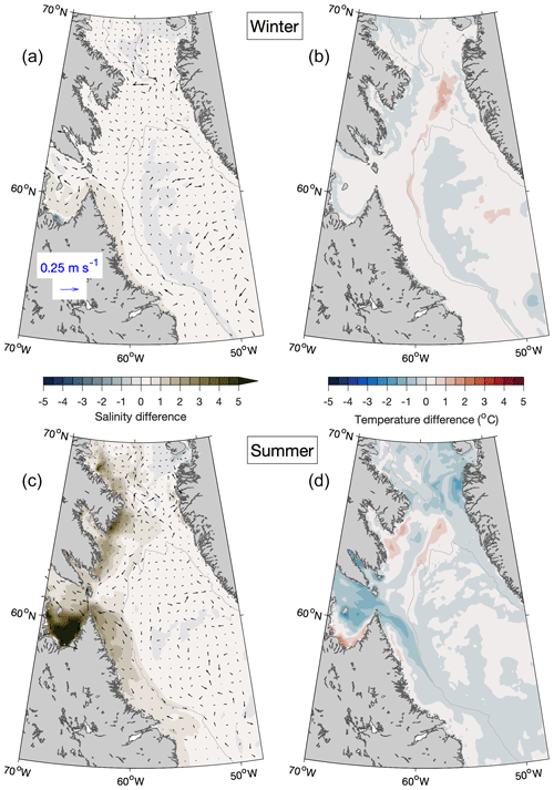
Figure 17 Differences in seasonal-mean simulated sea surface salinity and currents (a, c) and temperature (b, d) over Baffin Bay and the Labrador Sea when model results from NoTides are subtracted from those from Prog, averaged over winters (a, b) and summers (c, d) of 2015–2018. Difference vectors are shown at every 12th model grid point. The grey contour line represents the 1000 m water depth.

4.1 The effect of tides

Differences between Prog and NoTides (Prog minus NoTides) in sea surface salinity, currents, and temperature over Baffin Bay and the Labrador Sea, averaged over the winters (December–February) and summers (June–August) of December 2014–August 2018, are shown in Fig. 17. In winter (Fig. 17a, b), differences between the simulations of temperature and salinity over this area are relatively small – generally within ±1 for salinity, and up to $\sim +\mathrm{1.5}$ °C for temperature. In summer (Fig. 17c, d), $\mathrm{\Delta }{S}_{\mathrm{sfc}}^{\mathrm{P}-\mathrm{NT}}$ is positive along most of the Baffin Island coast, in Ungava Bay, and on the northern Labrador Shelf (up to ∼7 in Ungava Bay) while $\mathrm{\Delta }{T}_{\mathrm{sfc}}^{\mathrm{P}-\mathrm{NT}}$ is mostly negative throughout the area but especially over shelves (ca. −1.0 °C). These differences between Prog and NoTides are consistent with the presence of sea ice over large portions of this area during winter, given that sea ice can modulate tidal mixing and thus tends to reduce the differences between the ocean states simulated with and without tides. In summer, the presence of tidal mixing in Prog contributes to vertical mixing over shelf areas, resulting in surface waters that are saltier and colder than if there were no tides and the water column were more highly stratified. There are, however, areas in which the inclusion of tides results in positive $\mathrm{\Delta }{T}_{\mathrm{sfc}}^{\mathrm{P}-\mathrm{NT}}$ during the summer, notably along the coast of Ungava Bay. Given that $\mathrm{\Delta }{S}_{\mathrm{sfc}}^{\mathrm{P}-\mathrm{NT}}$ is positive throughout the bay, the contrast between positive $\mathrm{\Delta }{T}_{\mathrm{sfc}}^{\mathrm{P}-\mathrm{NT}}$ along the coast and negative $\mathrm{\Delta }{T}_{\mathrm{sfc}}^{\mathrm{P}-\mathrm{NT}}$ near the bay's mouth suggests air–sea fluxes might differ between the two parts of the bay.

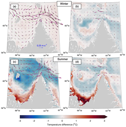
Figure 18 Differences between Prog and NoTides over Ungava Bay: 2015–2018 averages of seasonal-mean simulated currents (thick magenta arrows: Prog; thin green arrows: NoTides) and temperature difference (Prog minus NoTides) at the sea surface (a, c) and bottom layer (b, d) in winter (a, b) and summer (c, d). Current vectors are shown at every sixth model grid point. The grey contour line represents the 100 m water depth.

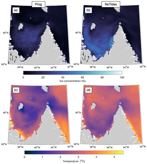
Figure 19 The 2015–2018 averages of seasonal-mean sea ice concentrations in Ungava Bay during summer simulated in the Prog (a) and NoTides (b) runs; seasonal-mean sea surface temperature for summer simulated by the Prog (c) and NoTides (d) runs.

The effect of tides on water temperature within Ungava Bay is explored in Figs. 18 and 19. In winter, the model results from Prog and NoTides are similar not only in terms of the surface temperature (Fig. 18a), but also in terms of bottom temperature ($\left|\mathrm{\Delta }{T}_{\mathrm{btm}}^{\mathrm{P}-\mathrm{NT}}\right|<\sim \mathrm{1.0}$ °C, Fig. 18b) and current speeds at both the surface and the bottom ($\mathrm{\Delta }{\left|\mathit{V}\right|}_{\mathrm{sfc}}^{\mathrm{P}-\mathrm{NT}}$ and $\mathrm{\Delta }{\left|\mathit{V}\right|}_{\mathrm{btm}}^{\mathrm{P}-\mathrm{NT}}<\sim \mathrm{0.1}$ m s⁻¹, Fig. 18a and b). In summer at the sea surface (Fig. 18c), both $\mathrm{\Delta }{\left|\mathit{V}\right|}_{\mathrm{sfc}}^{\mathrm{P}-\mathrm{NT}}$ and $\mathrm{\Delta }{T}_{\mathrm{sfc}}^{\mathrm{P}-\mathrm{NT}}$ are positive along the coast but generally negative in the outer bay. Along the bottom in summer (Fig. 18d), $\mathrm{\Delta }{T}_{\mathrm{btm}}^{\mathrm{P}-\mathrm{NT}}$ is positive and as large as ca. +4 °C along the coast, while in the outer bay $\mathrm{\Delta }{T}_{\mathrm{btm}}^{\mathrm{P}-\mathrm{NT}}$ is small ($\left|\mathrm{\Delta }{T}_{\mathrm{btm}}^{\mathrm{P}-\mathrm{NT}}\right|<\sim \mathrm{1.0}$ °C) and the currents are generally weak in both simulations. The patterns of mean summer sea ice concentration are also different between the two simulations, with the ice cover produced in Prog (Fig. 19a) being highest over the outer bay (up to ∼40 %) and low near the coast, while NoTides (Fig. 19b) produces a wide area of high ice cover along the coast (up to ∼90 %). The patterns of mean summer sea surface temperature from the two simulations (Fig. 19c, d) correspond to those of the sea ice cover, with areas of higher (lower) ice cover corresponding to lower (higher) temperatures. Given that the only difference between the Prog and NoTides simulations is the inclusion of tides in the former, these results suggest that tides along the coast of Ungava Bay promotes an earlier disappearance of ice there during the summer, and this in turn leads to a larger flux of solar radiation into the ocean and a less impeded flow.

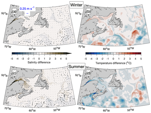
Figure 20 Similar to Fig. 17 but for the area between the Gulf of Maine and the southern Labrador Sea.

The effect of tides is also evident in the region surrounding two other areas with large tidal ranges, the St. Lawrence Estuary and the Bay of Fundy. In both winter and summer, $\mathrm{\Delta }{S}_{\mathrm{sfc}}^{\mathrm{P}-\mathrm{NT}}$ in the St. Lawrence Estuary (Fig. 20a, c) is positive (up to ∼6.0 in most of the estuary but >10 in parts of the upper estuary during the summer), suggesting that tidal mixing brings higher-salinity subsurface water towards the surface. In summer (Fig. 20c), the influence of this higher salinity due to tidal mixing spreads into the northwest Gulf of St. Lawrence due to the propagation of the estuarine plume. In the Bay of Fundy, the salinity difference is also positive in both seasons. In winter, $\mathrm{\Delta }{S}_{\mathrm{sfc}}^{\mathrm{P}-\mathrm{NT}}$ ranges from ∼0.4 in most of the bay to ∼2.4 near the Saint John River mouth, and in summer, it ranges from ∼1.2 in the upper bay to ∼3.6 near the Saint John River mouth. The role of tidal mixing is also evident in the patterns of sea surface temperatures (Fig. 20b, d), with $\mathrm{\Delta }{T}_{\mathrm{sfc}}^{\mathrm{P}-\mathrm{NT}}$ positive in winter (up to ∼1.5 °C in both the St. Lawrence Estuary and the Bay of Fundy) and negative in summer (as low as ca. −4.5 °C in both areas). Differences between the simulations are also visible over the open ocean for all three fields. As Wang et al. (2020) have suggested, this may be caused by internal tides that are generated near the shelf break and propagate offshore.

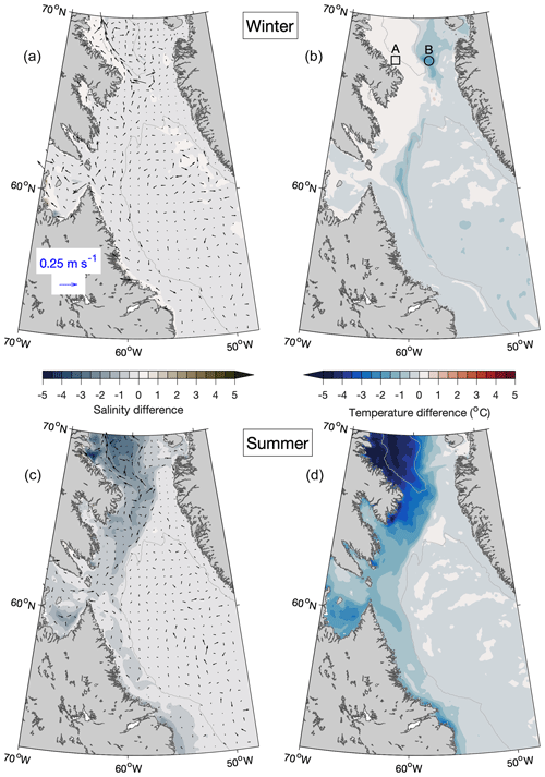
Figure 21 Differences in seasonal-mean simulated sea surface salinity and currents (a, c) and temperature (b, d) over Baffin Bay and the Labrador Sea where results of NoIce are subtracted from those of Prog, averaged over the winters (a, b) and summers (c, d) of 2015–2018. Difference vectors are shown at every 12th model grid point. The grey contour line represents the 1000 m water depth. Locations A and B, for which the vertical profiles of model variables are shown in Figs. 22 and 23, are indicated in panel (b) with a square and a circle, respectively.

4.2 The effect of sea ice

The effect of sea ice is examined next by comparing simulated surface fields from Prog to those from the simulation in which ROMS is run without coupling to CICE (NoIce). A prominent feature in winter is the horizontal gradient in $\mathrm{\Delta }{S}_{\mathrm{sfc}}^{\mathrm{P}-\mathrm{NI}}$, approximately aligned with the 1000 m isobath, in western Baffin Bay (Fig. 21a). $\mathrm{\Delta }{S}_{\mathrm{sfc}}^{\mathrm{P}-\mathrm{NI}}$ is positive on the shelf (ca. 0.2) but negative offshore of the shelf break (ca. −0.3). In the zone where $\mathrm{\Delta }{S}_{\mathrm{sfc}}^{\mathrm{P}-\mathrm{NI}}$ changes signs, $\mathrm{\Delta }{\left|\mathit{V}\right|}_{\mathrm{sfc}}^{\mathrm{P}-\mathrm{NI}}$ is positive (up to ∼0.3 m s⁻¹). The area on the shelf where $\mathrm{\Delta }{S}_{\mathrm{sfc}}^{\mathrm{P}-\mathrm{NI}}$ is positive coincides with the highest average sea ice thickness in the domain (Fig. 10d), which makes the higher salinity in Prog consistent with brine rejection at the time of sea ice formation. Values of $\left|\mathrm{\Delta }{T}_{\mathrm{sfc}}^{\mathrm{P}-\mathrm{NI}}\right|$ in winter (Fig. 21b) tend to be largest over the parts of Baffin Bay and the northern Labrador Shelf where the ice edge occurs in Prog (Fig. 10c). $\mathrm{\Delta }{T}_{\mathrm{sfc}}^{\mathrm{P}-\mathrm{NI}}$ values in these areas are negative (as low as ca. −1.9 °C). Surface heat flux is expected to result in positive $\mathrm{\Delta }{T}_{\mathrm{sfc}}^{\mathrm{P}-\mathrm{NI}}$, given that in winter it is expected to cool the ocean surface while sea ice can insulate the ocean surface below from cold air. Another possible factor in $\mathrm{\Delta }{T}_{\mathrm{sfc}}^{\mathrm{P}-\mathrm{NI}}$ is vertical mixing, which is examined later.

In summer, $\mathrm{\Delta }{S}_{\mathrm{sfc}}^{\mathrm{P}-\mathrm{NI}}$ and $\mathrm{\Delta }{T}_{\mathrm{sfc}}^{\mathrm{P}-\mathrm{NI}}$ (Fig. 21c and d, respectively) are lowest in western Baffin Bay, with the former as low as ca. −4.0 psu (reflecting the input of fresh water due to melting sea ice) and the latter as low as ca. −4.7 °C (reflecting the blocking of shortwave radiation by the sea ice that remains in summer). These results suggest that, as sea ice in areas such as Baffin Bay and the Labrador Shelf declines in a warming climate, areas downstream of them such as the Scotian Shelf and the Gulf of Maine will experience changes in the temperature and salinity of the water that is brought there by the Labrador Current. The effect of changes in water masses advected into a given area, in combination with changes that occur in situ due to climate change, is another possible topic of future research.

Differences in the wintertime vertical stratification and vertical mixing between Prog and NoIce are examined further using vertical profiles of 4-year mean wintertime temperature, salinity, and vertical eddy viscosity produced by the two runs, as well as the squared buoyancy frequency (N²) calculated from the mean wintertime temperature and salinity using the Gibbs-SeaWater Oceanographic Toolbox (McDougall and Barker, 2011). The profiles represent temporal averages over the same period as in Fig. 21a and b (winters of 2015–2018) and are calculated at 1 m depth intervals for two locations: location A (67.60° N, 62.56° W), indicated by the square in Fig. 21b, where $\mathrm{\Delta }{T}_{\mathrm{sfc}}^{\mathrm{P}-\mathrm{NI}}$ is small and the 2015–2018 mean of the February mean sea ice cover is ∼95 % (Fig. 10c), and location B (67.60° N, 57.64° W), indicated by the circle in Fig. 21b, where $\mathrm{\Delta }{T}_{\mathrm{sfc}}^{\mathrm{P}-\mathrm{NI}}$ has a large magnitude (ca. −1.9 °C) and the 4-year mean of the February mean sea ice cover is ∼84 %. The model's water depths at the two locations are similar (231 and 218 m).

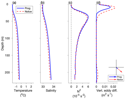
Figure 22 Vertical profiles of wintertime temperature (a), salinity (b), squared buoyancy frequency (c), and vertical eddy diffusivity (d) simulated by the model in Prog (solid blue line) and NoIce (dashed red line), averaged over 2015–2018, interpolated to 1 m depth intervals, at location A, indicated by the square in Fig. 21b (67.60° N, 62.56° W). Also shown in panel (d) is the stress exerted on the sea surface by sea ice and/or winds in the Prog (thick arrow) and NoIce (thin arrow) runs, averaged over the same period as the other fields. The x and y axes for the surface stress range from −0.1 to 0.1 N m⁻².

The vertical profiles of mean wintertime temperature (Fig. 22a) and salinity (Fig. 22b) at location A are similar between the Prog and NoIce runs, with a vertical range of <1.4 °C for temperature and <0.8 for salinity in both runs. The profiles of N² (Fig. 22c) are thus also similar between the runs, with maximum values of $\sim \mathrm{6}\times {\mathrm{10}}^{-\mathrm{5}}$ s⁻² about 40 m below the sea surface. Negative values of N², indicating instability, are limited to the top few metres of the water column. Values of the Richardson number (not shown) below 0.25, including negative values, are limited to the top 5 m of the water column, again indicating a mostly stable water column and weak convection in both Prog and NoIce. The mean wintertime vertical mixing below the surface is very weak in both runs (Fig. 22d), with the vertical eddy diffusivity from both runs having maximum values of ∼0.02 m² s⁻¹ about 10 m below the surface and having values of <0.002 m² s⁻¹ in ∼80 % of the water column. It should be noted that the mean wintertime stress exerted on the sea surface (by winds and/or sea ice in Prog and by winds in NoIce) differs significantly between the two runs (Fig. 22d). The surface stress has a much smaller magnitude in Prog (0.02 N m⁻²) than in NoIce (1.0 N m⁻²), which can be explained by the buffering effect of sea ice on the wind stress in Prog. Due to this buffering effect of sea ice, the wind-induced vertical mixing in the surface layer (Fig. 22d) is weaker in Prog than in NoIce, as expected.

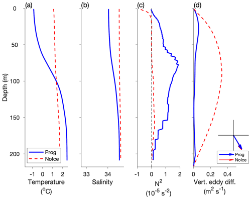
Figure 23 Similar to Fig. 22 but for location B, indicated by the circle in Fig. 21b (67.60° N, 57.64° W). Note the change from Fig. 22 in the x-axis limits for the squared buoyancy frequency (c) and the vertical eddy diffusivity (d).

In contrast to location A, the vertical profiles of mean wintertime model results at location B differ significantly between the Prog and NoIce runs. The mean wintertime temperature (Fig. 23a) has a vertical range of >3 °C in Prog (about −0.9 °C near the surface and 2.4 °C near the bottom) but <1.0 °C in NoIce (about 1.1 °C near the surface and 1.7 °C near the bottom). The mean wintertime salinity (Fig. 23b) has a vertical range of ∼0.5 in Prog (about 34.0 near the surface and 34.5 near the bottom) but just ∼0.1 in NoIce (about 34.5 near the surface and 34.6 near the bottom). Values of N² (Fig. 23c) from both runs are lower than at location A, with a maximum of $\sim \mathrm{1.9}\times {\mathrm{10}}^{-\mathrm{5}}$ s⁻² in Prog and $\sim \mathrm{2.1}\times {\mathrm{10}}^{-\mathrm{6}}$ s⁻² in NoIce. In addition, the N² in NoIce is negative in the top ∼20 m of the water column and between depths of ∼40 and ∼50 m, indicating unstable stratification and unrealistically strong convection. The Richardson number is <0.25 in the top ∼5 m of the water column in Prog and at approximately the same depths as where the negative values of N² are in NoIce. The maximum vertical eddy diffusivity coefficient is ∼0.3 m² s⁻¹ in NoIce, which is much larger than the maximum values of ∼0.06 m² s⁻¹ in Prog, while the surface stress is similar at ∼0.1 N m⁻² in both runs.

A possible explanation for the relatively warm (>2.0 °C) and salty (>34.0 psu) subsurface water in the lower water column at location B in Prog (solid blue lines in Fig. 23a, b) is the horizontal advection of relatively warm and salty waters from the south to this location. In Prog, the ocean-to-air heat flux in winter results in cooling of the near-surface water as well as in sea ice formation, and subsurface ablation of the sea ice can be a source of fresh water that contributes to vertical stability. The advection of relatively warm, salty subsurface waters from the south would also occur in NoIce, but in this case the near-surface water would be cooled to the freezing point without an accompanying reduction in salinity, which may explain the very large vertical mixing and nearly uniform vertical profiles of temperature and salinity in this run.

5 Conclusions

In this study, a newly developed, fully coupled modelling system for simulating the ocean circulation, sea ice, and biogeochemistry of the northwest Atlantic Ocean (DalROMS-NWA12 v1.0) was described. The model domain covers the area from Cape Hatteras to Baffin Bay with a horizontal resolution of ∼2 to ∼8 km, making this modelling system highly suitable for a range of research topics, including study of the biological carbon pump and quantification of the major physical and biogeochemical (BGC) processes influencing the ocean carbon cycle over the region. The results of two simulations using this modelling system, with and without nudging of the simulated temperature and salinity towards a blend of observations and reanalysis, were compared to observations and reanalysis. We found that results of the control run, which included the nudging, are more realistic than results of the prognostic (un-nudged) simulation for several important physical features observed in this region, such as separation of the Gulf Stream and the West Greenland Current from their respective coasts, as well as propagation of low-salinity waters from the St. Lawrence Estuary. These results demonstrate the utility of simple data assimilation in reducing the systematic model errors that can be attributed to model configuration (such as horizontal grid resolution in the case of currents' separation from coasts and the choice of tracer advection scheme in the case of estuarine plume propagation) and unresolved or parameterized physical and BGC processes. The prognostic simulation, while having difficulties with the above-mentioned features, was able to reproduce the general spatiotemporal patterns of the physical fields and outperformed the control run in terms of the sea ice concentration. The major differences between the simulations in the sea ice extent highlight the complex nature of interactions among the atmosphere, ocean, and sea ice.

The modelling system was able to reproduce the general patterns of BGC variables over the northwest Atlantic shelves and in the Labrador Sea. Further validation will include comparisons with observations made by BGC Argo floats (Johnson and Claustre, 2016). Future work will use this modelling system to investigate the biological carbon pump in the Labrador Sea including vertical flux estimates derived from BGC Argo (Wang and Fennel, 2022, 2023). The addition of silicate as a state variable will also be tested.

As an example of an application of this modelling system, sensitivity studies were made in which results of the prognostic simulation were compared to those from similar simulations from which either the tides or simulation of sea ice was excluded. The comparisons suggest that tides and sea ice strongly affect the physical oceanography of the northwest Atlantic Ocean (NWA) in several ways. These include the combined effects of tides and sea ice (in Ungava Bay) as well as individual effects (e.g., higher surface salinity in summer when sea ice is not simulated).

In addition to studies of the biological carbon pump and of the downstream effects of changes in the water transported by the Labrador Current, another possible direction of future research is to further explore the effects of model configuration, such as parameterization of deep convection or the choice of advection schemes (including the use of non-zero horizontal eddy diffusivity and viscosity with the third-order upstream scheme). In addition, we can use the ocean state simulated by this model as input for numerical particle-tracking experiments to investigate connectivity among different areas of the NWA. The resulting metrics of connectivity under current and projected future climate conditions can support decision-making processes concerning conservation measures. The model will also be used to compare approaches to reducing bias in long-term simulations.

The high air-to-sea flux of CO₂ and the subsequent downward export of fixed carbon make the NWA a key component in the global climate system, but it is a remote region where seasonal transitions can take place in just a few weeks (e.g., in terms of pCO₂; Körtzinger et al., 2008), and details of the interactions between physical and biogeochemical processes are still unknown or remain poorly integrated into models (e.g., the sea ice carbon pump; Richaud et al., 2023). The four-dimensional ocean states produced by numerical models can aid in the interpretation of observations as well as enabling experiments that elucidate the roles of various processes in the ocean and possible changes to those processes under future climate scenarios. As part of our future studies, this advanced coupled modelling system will be run for longer simulation periods to examine the effects of climate change on the marine conditions over the NWA. The modelling system will also be used to predict the temporal and spatial variability in future marine conditions over the region under different climate scenarios.

Appendix A: The vertical coordinate system in ROMS

ROMS uses a generalized terrain-following vertical coordinate system with several options for vertical transformation equations and vertical stretching functions. In this study the default configuration is used, with the vertical coordinate S defined as (Hedstrom, 2018)

$$\begin{array}{}\text{(A1)}& {\displaystyle }\begin{array}{rl}z\left(x,y,\mathit{\sigma },t\right)& =\mathit{\zeta }\left(x,y,t\right)\\ & +\left[\mathit{\zeta }\left(x,y,t\right)+h\left(x,y\right)\right]S\left(xy\mathit{\sigma }\right),\end{array}\text{(A2)}& {\displaystyle }S\left(x,y,\mathit{\sigma }\right)={\displaystyle \frac{h_{\mathrm{c}}+h\left(x,y\right)C\left(\mathit{\sigma }\right)}{h_{\mathrm{c}}+h(x,y)}},\text{(A3)}& {\displaystyle }C\left(\mathit{\sigma }\right)={\displaystyle \frac{\exp ({\mathit{\theta }}_{\mathrm{b}}{C}^{\prime }\left(\mathit{\sigma }\right)-\mathrm{1}}{\mathrm{1}-\exp (-{\mathit{\theta }}_{\mathrm{b}})}},\text{(A4)}& {\displaystyle }{C}^{\prime }\left(\mathit{\sigma }\right)={\displaystyle \frac{\mathrm{1}-\cosh \left({\mathit{\theta }}_{\mathrm{s}}\mathit{\sigma }\right)}{\cosh \left({\mathit{\theta }}_{\mathrm{s}}\right)-\mathrm{1}}},\end{array}$$

where σ ranges from 0 at the free surface to −1 at the ocean bottom; ζ is the free surface; h is the undisturbed water column thickness; h_c is the value of h below which the vertical layers are more uniformly spaced; and θ_s and θ_b are parameters that control the vertical resolution near the surface and the bottom, respectively. In this study ROMS has 40 layers and the parameters h_c, θ_s, and θ_b are set to 100 m, 5.0, and 0.5, respectively.

Appendix B: Seasonal-mean simulated fields

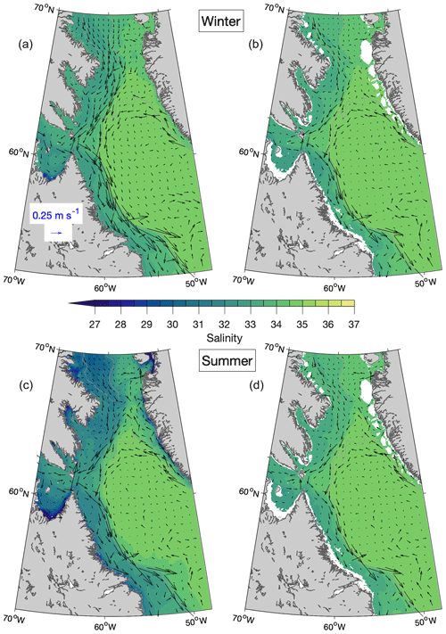
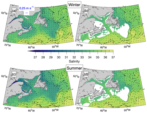
Seasonal means of salinity and currents in Baffin Bay and the northern Labrador Sea simulated in Ctrl and Prog, averaged over the period December 2014–December 2018, are shown in Figs. B1 and B2. Differences between the simulations are more evident in summer (June–August; Figs. B1c–d and B2c–d) than in winter (December–February; Figs. B1a–b and B2a–b). The Baffin Island Current and the northward branch of the West Greenland Current are stronger in Prog by up to ∼0.25 m s⁻¹ at the surface and ∼0.15 m s⁻¹ for model results interpolated to the 100 m depth. In the area between the southern Labrador Sea and the Gulf of Maine (Figs. B3 and B4), the difference in salinity between the simulations is more prominent in summer, following the annual peak in freshwater discharges from the St. Lawrence and other rivers. In the St. Lawrence Estuary, the 2015–2018 mean of summer surface salinity simulated in Prog is lower than that from Ctrl by up to ∼3.5, but further downstream in the Gulf of St. Lawrence, the salinity from Prog is higher by ∼2.

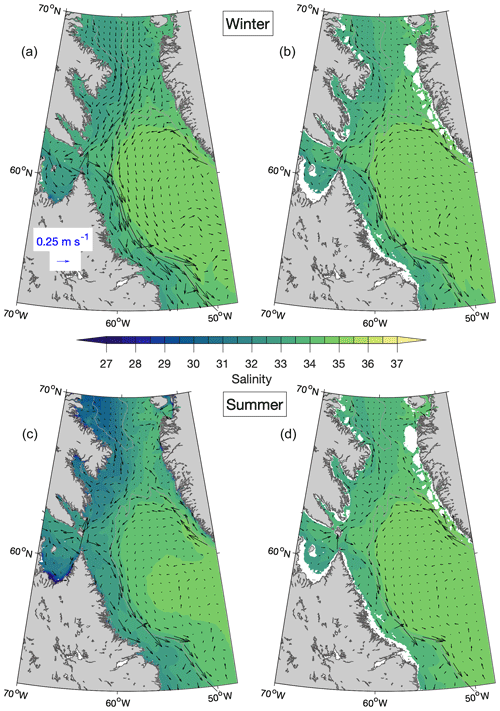
Figure B1 Seasonal-mean simulated salinity and currents at the sea surface (a, c) and interpolated to the 100 m depth (b, d) from Ctrl averaged over the winters (a, b) and summers (c, d) of 2015–2018 in Baffin Bay and the Labrador Sea. Winters are defined as December of the previous year to February of that year. Summers are defined as June to August. Current vectors are shown at every 12th grid point. The grey contour line represents the 1000 m water depth.

Figure B2 Similar to Fig. B1 but for Prog.

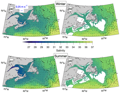
Figure B3 Seasonal-mean simulated salinity and currents at the sea surface (a, c) and interpolated to the 100 m depth (b, d) from Ctrl averaged over the winters (a, b) and summers (c, d) of 2015–2018 over the area between the Gulf of Maine and the southern Labrador Sea. Current vectors are shown at every 12th grid point. The 1000 m depth contour is shown in grey.

Figure B4 Similar to Fig. B3 but for Prog.

Appendix C: Data sets used in model performance assessment

Online sources of the data sets used to assess the model performance are listed below in the order they are discussed in Sect. 3.

1. Sea surface temperature. OISST v2.1 (Huang et al., 2021) is a daily data set on a $\mathrm{1}/\mathrm{4}$° grid that incorporates satellite and in situ observations. A combination of v2.0 and v2.1 was used in this study; v2.0 is now retired (https://www.ncei.noaa.gov/products/optimum-interpolation-sst, last access: 26 November 2024).

2. Sea surface salinity. MULTIOBS_GLO_PHY_S_SURFACE_MYNRT_015_013 (Buongiorno Nardelli et al., 2016) is a data set that incorporates satellite and in situ observations. At the time of this study, it was a weekly data set on a $\mathrm{1}/\mathrm{4}$° grid; now it is a daily data set on a $\mathrm{1}/\mathrm{8}$° grid (https://data.marine.copernicus.eu/product/MULTIOBS_GLO_PHY_S_SURFACE_MYNRT_015_013/description, last access: 26 November 2024).

3. Currents. GLOBAL_MULTIYEAR_PHY_001_030, also known as GLORYS12V1 (Lellouche et al., 2021), is a daily reanalysis data set on a $\mathrm{1}/\mathrm{12}$° grid (https://data.marine.copernicus.eu/product/GLOBAL_MULTIYEAR_PHY_001_030/description, last access: 26 November 2024).

4. Shipboard observations of physical and biogeochemical variables. Atlantic Zone Monitoring Program (Pepin et al., 2005) cruises take place seasonally and Atlantic Zone Off-Shelf Monitoring Program (e.g., Yashayaev and Loder, 2017) cruises take place annually (https://catalogue.cioosatlantic.ca/dataset/ca-cioos_9a4bd73f-12a2-40ff-a7c7-b961a1d11311, last access: 26 November 2024, https://catalogue.cioosatlantic.ca/dataset/ca-cioos_15f90eab-21ed-447d-aea7-8fe98ea27fe5, last access: 26 November 2024).

5. Sea ice. AMSR2 ASI sea ice concentration data for the Arctic, v5.4 (Melsheimer and Spreen, 2019), are from a daily data set on a 6.5 km grid derived from satellite observations (https://doi.org/10.1594/PANGAEA.898399).