Evaluating downscaled products with expected hydroclimatic co-variances

There has been widespread adoption of downscaled products amongst practitioners and stakeholders to ascertain risk from climate hazards at the local scale (e.g., ∼ 5 km resolution). Such products must nevertheless be consistent with physical laws to be credible and of value to users. Here we evaluate statistically and dynamically downscaled products by examining local co-evolution of downscaled temperature and precipitation during convective and frontal precipitation events (two mechanisms testable with just temperature and precipitation). We find that two widely used statistical downscaling techniques (Localized Constructed Analogs version 2, LOCA2, and Seasonal Trends and Analysis of Residuals Empirical Statistical Downscaling Model, STAR-ESDM) generally preserve expected co-variances during convective precipitation events over the historical and future projected intervals as compared to European Centre for Medium-Range Weather Forecasts Reanalysis v5 (ERA5) and two observation-based data products (Livneh and nClimGrid-Daily). However, both techniques dampen future intensification of frontal precipitation that is otherwise robustly captured in global climate models (i.e., prior to downscaling) and with process-based dynamical downscaling across five different regional climate models. In the case of LOCA2, this leads to appreciable underestimation of future frontal precipitation event intensity. This study is one of the first to quantify a likely ramification of the stationarity assumption underlying statistical downscaling methods and identify a phenomenon where projections of future change diverge depending on data production method employed. Finally, our work proposes expected co-variances during convective and frontal precipitation as useful evaluation diagnostics that can be universally applied to a wide range of statistically downscaled products.

1 Introduction

Extreme weather events are among the costliest disasters to the United States. Over the past 4 decades (1980–2023), there have been more than 370 billion-dollar disasters that cumulatively cost over 2.6 trillion dollars (NOAA, 2024). To ascertain risk from climate hazards, a broad community of practitioners, stakeholders, and policymakers rely on historical reconstructions and future projections of local to regional climate that are “downscaled” from coarse global climate model outputs (Fiedler et al., 2021; Pitman et al., 2022). This is because global climate model (GCM) data alone are too coarse in resolution: GCM outputs from the Coupled Model Intercomparison Project 6 (CMIP6), for instance, have a grid spacing of ∼ 100 to 300 km in the midlatitudes and cannot adequately represent finer-scale features like topography and extreme storms (Eyring et al., 2016).

Numerous climate data products have emerged over the last several years that represent the contiguous United States (herein CONUS) at local scales, including dynamically and statistically downscaled products. Dynamically downscaled products (e.g., Jones et al., 2023; Liu et al., 2017; Dai et al., 2020; Rasmussen et al., 2023; Chen et al., 2023) use regional climate models that simulate local meteorology, providing a comprehensive set of climate variables that are inherently self-consistent. While the general expectation is that dynamical downscaling implicitly preserves physical relationships among variables because they are generated by a modeling system based on physical laws, it is known that some biases can arise from insufficient representation of relevant physical processes (such as eddies; Xu et al., 2019), inherent error from lateral boundary input (e.g., from GCMs; Rahimi et al., 2024), and/or sensitivity to regional climate model configurations (the limitations of regional climate models were comprehensively reviewed by Giorgi, 2019, and Lloyd et al., 2021) that must be considered. Statistically downscaled products (e.g., Abatzoglou and Brown, 2012; Thrasher et al., 2012, 2022; Pierce et al., 2014, 2023) are derived based on relationships between coarse climate model outputs and observed local meteorology (e.g., Livneh et al., 2015a; Durre et al., 2022a). Since they are generated through simple functional relationships, statistically downscaled products can be generated more rapidly than dynamically downscaled products (albeit for fewer variables as dense observational networks are only available for select quantities).

Given their computational convenience, there has been widespread adoption of statistically downscaled products. Statistically downscaled products must nevertheless be credible to be of value to users; the data must be consistent with physical laws to be trusted for future projections (Cash et al., 2002). Importantly, common statistical downscaling methods downscale variables independently of one another and thus do not explicitly account for co-variances across variables at the local scale (notwithstanding existing co-variances generated by climate models prior to downscaling). This may be problematic as the loss of process-relevant co-variances, if any, would undermine downstream assessments of multi-variate hazards (e.g., droughts, flooding, and wildfires). Drought and wildfire metrics, for instance, may require self-consistent inputs of temperature and precipitation. Additionally, statistical downscaling assumes that observed functional relationships will be preserved in the future (i.e., the stationarity assumption) despite climate change (Milly et al., 2008); however, there is no guarantee that historically derived statistical relationships will remain valid in the future. A precise understanding of the extent to which such an assumption may undermine projections nevertheless remains elusive.

Here we assess the extent to which two locally relevant co-variances between temperature and precipitation are preserved (or lost), as compared to outputs from global climate models and their dynamically downscaled counterparts, in two widely used (e.g., Martin, 2023; Ullrich, 2023; Najibi et al., 2024; Wang et al., 2024) statistical downscaling techniques selected to accompany the Fifth National Climate Assessment (NCA5; the pre-eminent guidance on national climate risks; USGCRP, 2023): Localized Constructed Analogs version 2 (LOCA2; Pierce et al., 2023) and Seasonal Trends and Analysis of Residuals Empirical Statistical Downscaling Model (STAR-ESDM; Hayhoe et al., 2024). A central goal of our paper is to understand the representation of physical mechanisms in statistical downscaling products with only daily surface temperature and precipitation outputs (often the only two variables available with statistical downscaling). For this reason, we examine expected co-variances between temperature and precipitation during convective and frontal precipitation events, including for the projection interval, where the stationarity assumption may not hold. Although the credibility of both LOCA2 and STAR-ESDM has been evaluated for single variables (e.g., Pierce et al., 2023; Hayhoe et al., 2024), we propose, for the first time, diagnostics for evaluating co-variances that can be universally applied to a wide range of statistically downscaled products. Collectively, our work attempts to address the following questions:

To what extent is physical consistency across variables preserved, as compared to observations, when variables are (i) statistically downscaled independently and (ii) dynamically downscaled concurrently?

How much does the stationarity assumption inherent in statistical downscaling undermine credibility of projections, particularly for potentially non-stationary hydrologic processes?

2 Data and methods

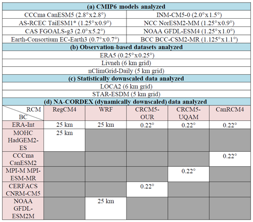
We employ outputs from eight Coupled Model Intercomparison Project Phase 6 (CMIP6) models and their statistically downscaled counterparts (see Table 1). The statistically downscaled products come from Localized Constructed Analogs version 2 (LOCA2; Pierce et al., 2023) and Seasonal Trends and Analysis of Residuals Empirical Statistical Downscaling Model (STAR-ESDM; Hayhoe et al., 2024). The following description of LOCA2 and STAR-ESDM is from Ullrich (2023), with minor modifications. LOCA2 is a statistical downscaling technique based on signal decomposition employing analogs (i.e., days in the historical record that exhibit regional meteorology most like the regional patterns of a given day in the CMIP6 model). The LOCA2 algorithm first bias-corrects historical CMIP6 outputs to observations using quantile mapping. It then adjusts the amount of variability seen in different frequency bands to match observations using a digital filter (Pierce et al., 2014, 2023). To downscale data at a given grid cell, the 30 d period in the historical record best exhibiting regional meteorology as compared to the CMIP6 model day is identified. The single day best matching the model day is used as the analog for the local region around the grid point (Pierce et al., 2023). The LOCA2 North American product uses an updated version of Livneh et al. (2015a) with 6 km grid spacing as the training dataset (Pierce et al., 2021). Outputs from LOCA2 are also available at 6 km grid resolution.

Table 1 (a) List of CMIP6 models analyzed. All models use the r1i1p1f1 member. We examine the same eight models in the LOCA2 and STAR-ESDM downscaled data. ^* TaiESM1 is only analyzed over the historical interval (and not the future interval) for the raw GCM due to data availability. Longitude-by-latitude grid resolution is provided in parentheses (rounded to nearest $\mathrm{1}/\mathrm{10}$th of a degree except in cases where resolution ends exactly in a quarter or eighth of a degree). (b) List of observation-based datasets analyzed. (c) List of statistically downscaled datasets analyzed. (d) Simulation matrix adapted from NA-CORDEX. The left column shows the underlying boundary condition (BC) data being dynamically downscaled. The top row shows the regional climate model (RCM) driving the downscaling. The simulations analyzed show the grid spacing of downscaled model. In addition to global climate models, NA-CORDEX downscales ERA-Interim (top of left column) across different regional climate models (this allows for a comparison of downscaling across a common dataset).

STAR-ESDM is a statistical downscaling technique based on signal decomposition (Hayhoe et al., 2024). The STAR-ESDM algorithm first disaggregates observations and GCM outputs into four separate components: the long-term trend, climatological annual cycle, annually varying annual cycle, and high-frequency daily anomalies. For each of these components, mappings are constructed between observations and historical GCM outputs. Future projections are bias-corrected using these mappings, and then components are recombined to produce a consistent estimate of future time series. The STAR-ESDM product uses nClimGrid-Daily data with 5 km grid spacing for training over CONUS (Durre et al., 2022a). Both the LOCA2 and STAR-ESDM datasets were chosen for operational use in the Fifth National Climate Assessment.

We compare convective and frontal precipitation processes (specifics of how these processes are defined are provided in subsequent paragraphs) from (i) the European Centre for Medium-Range Weather Forecasts Reanalysis fifth-generation data (ERA5; Hersbach et al., 2020) against (ii) CMIP6 GCMs and their statically downscaled counterparts (LOCA2 and STAR-ESDM). We also examine convective and frontal precipitation processes in the observation-based Livneh (Livneh et al., 2015a) and nClimGrid-Daily (Durre et al., 2022a) hydrometeorological datasets. Finally, to assess the extent to which the stationarity assumption affects projections across statistical and dynamical downscaling, we compare LOCA2 and STAR-ESMD against the North America component of the Coordinated Regional Downscaling Experiment (NA-CORDEX; Mearns et al., 2017). NA-CORDEX dynamically downscales ERA-Interim reanalysis data and climate model simulations under historical and Representative Concentration Pathway 8.5 W m⁻² (RCP8.5) forcings with a suite of regional climate models. We employ five different raw GCM experiments downscaled with five different regional climate models that provide daily outputs at ∼ 25 km resolution. See Table 1 for a summary of all the datasets examined in this paper.

Statistically downscaled products generally only provide a few variables at daily or higher frequencies, which can make it difficult to evaluate co-variances. Directly computing co-variance between temperature and precipitation at daily timescales may not be useful due to non-linear physical relationships and/or the stochastic nature of weather. We follow Zhang and Boos (2023) in isolating for a single convective precipitation event each year by considering precipitation at each grid point coincident with the highest daily maximum temperature during that year (herein convective precipitation). Similarly, we isolate for a single (cold) frontal precipitation event each year by considering precipitation coincident with the greatest drop in surface temperature for that year (herein convective precipitation). For every grid point, our method thus identifies one convective precipitation event and one frontal precipitation event per year. To evaluate our method of identifying precipitation events, we (i) identify grid by grid the calendar day of convective and frontal precipitation, respectively, for each year over 1980–2014, (ii) create histograms of the number of times that the day of convective or frontal precipitation falls between day 0 and day 365 of each year (days 0–365 are thus effectively histogram bins), and (iii) fit a discrete Fourier transform to the respective histogram to identify the dominant frequency (i.e., frequency corresponding to peak day) present in the data.

We examine daily near-surface temperature and precipitation fields on a per-grid basis during convective and frontal precipitation events over CONUS, focusing on a 21 d window from 10 d prior to and 10 d following the day of convective and frontal precipitation, respectively (and including the day of convective or frontal precipitation itself). For the raw GCMs and ERA5, we also examine moist static energy, which we estimate using daily temperature, specific humidity, and geopotential height but monthly surface pressure (due to data availability). For the purposes of this study, we examine (i) a 35-year period spanning the 1980–2014 historical interval and (ii) a 35-year period spanning the 2065–2099 interval under the Shared Socioeconomic Pathway “fossil-fueled development” scenario with 8.5 W m⁻² of radiative forcing (SSP585). For dynamical downscaling outputs, we examine the 2065–2098 interval under the RCP8.5 forcing (note that the years 2006–2014 fall under the RCP8.5 scenario for NA-CORDEX).

3 Results

3.1 Convective and frontal precipitation processes in observation-based datasets

We first examine convective precipitation in the ERA5 Reanalysis dataset (Fig. 1). Composite time series centered around the hottest day (day 0) show surface temperature anomalies increase exponentially from −1 K 10 d prior (day −10), peak at 3–4 K on the hottest day (day 0) and then decrease exponentially to −1 K after 10 d (day +10). Spatial composites of the hottest day show warm temperature anomalies over the CONUS domain, while the fifth day after shows broad cool anomalies. Coincident composite time series of precipitation show anomalies that decrease from day −10 to day 0 (co-occurring with temperature anomalies increasing). Precipitation anomalies are the lowest on the hottest day (between −1 and −1.5 mm d⁻¹), with the spatial composite of day 0 showing broad dryness. Precipitation anomalies increase rapidly in the immediate days following, coincident with rapid surface temperature anomaly decreases, and then remain elevated after the onset of convection. The spatial composite of precipitation on day + 5, for instance, shows broad wetting indicative of convective precipitation.

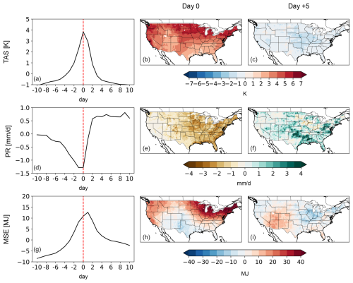
Figure 1 (a) The 21 d composite (spatially averaged over the contiguous US, CONUS, domain) time series of surface temperature anomalies (relative to the 21 d average) centered around the day of convective precipitation using ERA5 data over the 1980–2014 interval. (b) Spatial composite of surface temperature anomalies on the day of convective precipitation. (c) Spatial composite of surface temperature anomalies 5 d after convective precipitation. (d)–(f) Same as (a)–(c) but for precipitation. Note that these are anomalies relative to the 21 d window, yielding both positive and negative values. (g)–(i) Same as (a)–(c) but for moist static energy (MSE). Moist static energy increases until the precipitation event and rapidly decreases immediately afterwards as the atmosphere stabilizes.

The above co-evolution of surface temperature and precipitation are consistent with expectations of convective precipitation: surface temperature will rise until it convects, triggering precipitation and cooling surface temperature. Analysis of coincident moist static energy reinforces this mechanism: moist static energy increases until the precipitation event and rapidly decreases immediately afterwards as the atmosphere stabilizes (Fig. 1). Finally, our findings extend to the observation-based Livneh (Fig. S1) and nClimGrid-Daily (Fig. S2) datasets. Although observational climate datasets themselves have inherent uncertainties (such as from generation, sampling, or resolution; Zumwald et al., 2020), strong consistency across ERA5 and the two observation-based products indicate our ERA5 results to be robust.

We next examine cold frontal precipitation in ERA5, centered around the greatest drop in surface temperature (Fig. 2). Our selection of frontal precipitation events shows a very different relationship between temperature and precipitation as compared to convective precipitation. Composite time series show temperature anomalies to be the highest on the day of frontal precipitation (day 0), drop to the lowest in the following 2 days (day +1 to +2), and then return to ∼ 0 by day +10. Spatial composites of surface temperature show warm anomalies on day 0 and cold anomalies on day +2. Coincident precipitation time series show anomalies that increase dramatically (from <0 mm d⁻¹ at day −2 to ∼ 4 mm d⁻¹ at day 0) before falling back to <0 mm d⁻¹. Spatial composites of precipitation anomalies on day 0 show broad wetting, with the eastern half of CONUS showing greater anomalies; spatial composites on day +2 show largely neutral conditions over most of CONUS. Analysis of moist static energy reinforces a cold frontal precipitation mechanism, with a steep decline in moist static energy that is coincident with a steep decline in surface temperature and with sudden precipitation (Fig. 2).

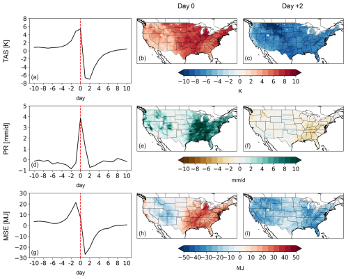
Figure 2 (a) The 21 d composite (spatially averaged over the CONUS domain) time series of surface temperature anomalies (relative to the 21 d average) centered around the day of cold frontal precipitation using ERA5 data over the 1980–2014 interval. (b) Spatial composite of surface temperature anomalies on the day of convective precipitation. (c) Spatial composite of surface temperature anomalies 2 d following the day of frontal precipitation. (d)–(f) Same as (a)–(c) but for precipitation. (g)–(i) Same as (a)–(c) but for moist static energy.

To further evaluate our method of identifying precipitation events, we apply a discrete Fourier transform on days of the year when the convective and frontal precipitation events are occurring, respectively (Fig. 3). We find that convective precipitation occurs predominantly in boreal summer (June–July–August; consistent with when warm days are prevalent). Frontal precipitation occurs predominantly in boreal winter (December–January–February; consistent with when cold fronts would be most prevalent), notwithstanding intermountain regions of the US west, where orographic lifting is prevalent (note that this is also the case with raw CMIP6 GCMs; Fig. S3). We also calculate kernel density estimates (KDEs) of precipitation anomalies before convection (day −2) and after convection (day +2) for the 35-year composite of convective precipitation events (Fig. 4); the two KDEs are significantly different (p<0.01; Kolmogorov–Smirov test). Moreover, we find 97 % of the CONUS grid points have higher precipitation anomalies at day +2 relative to day −2. We perform similar analyses for frontal precipitation: KDEs of precipitation anomalies during day +0 and day +1 are significantly different (p<0.01) from the rest of the 21 d window; 93 % of the maximum precipitation in our 35-year composite of events occurs on day +0 or day +1. Given the abovementioned co-variances, demonstrated skill in selecting for desired events, and expected seasonal occurrence of said events, we deem the physical relationships between surface temperature and precipitation observed in ERA5 during convective and frontal precipitation (as identified in our methodology) to be appropriate for evaluating the credibility of GCMs and their statistically downscaled products.

Figure 3 Peak convective and frontal day of year using the ERA5 dataset. Peak day is determined using a discrete Fourier transform.

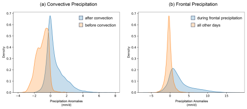
Figure 4 (a) Kernel density estimates (KDEs) of convective precipitation anomalies before convection (orange; day −2) and after convection (blue; day +2) for the 35-year composite of convective precipitation events. In total, 97 % of grid points during the 21 d analyzed show higher precipitation anomalies after convection. The two KDEs are significantly different (p<0.01) as determined by a Kolmogorov–Smirnov test. (b) KDEs of frontal precipitation anomalies on day +0 and day +1 (blue) and all other days of the 21 d window analyzed (orange; randomly sampled). Indeed, 93 % of the maximum precipitation occurs on day +0 or day +1. The two KDEs are significantly different (p<0.01) as determined by a Kolmogorov–Smirnov test.

3.2 Precipitation processes in raw and statistically downscaled GCMs over the historical interval

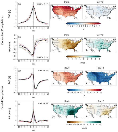
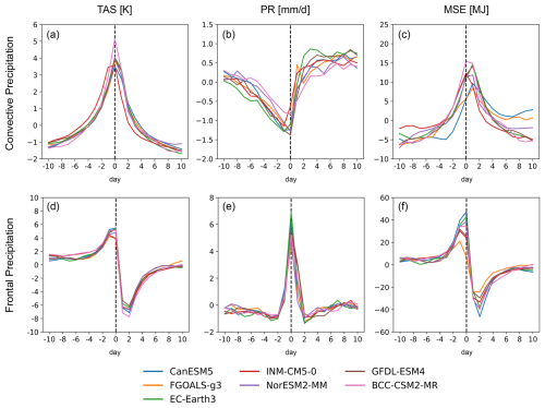
Some spread amongst the GCMs notwithstanding, the eight CMIP6 GCMs analyzed herein behave consistently with ERA5 for both convective and frontal precipitation over the 1980–2014 historical interval (Fig. 5; see Table 1 for list of models). That is, convective precipitation anomalies consistently (i) decrease leading up to the hottest day, (ii) are the lowest about the hottest day, and then (iii) drastically increase with convection in the immediate days following. Frontal precipitation is also clearly visible in the GCMs, with drastic and acute precipitation evident centered around the day of greatest temperature decrease. The raw GCMs not only match the temporal co-evolution of surface temperature and precipitation as demonstrated in ERA5 but also correctly simulate the magnitude of anomalies during convective and frontal precipitation events. Our results therefore indicate that the CMIP6 GCMs robustly capture convective and frontal precipitation processes.

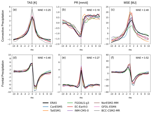
Figure 5 The 21 d composite time series (spatially averaged over CONUS domain) of (a) surface temperature (K), (b) precipitation (mm d⁻¹), and (c) moist static energy (MJ) anomalies (relative to the 21 d average) for raw CMIP6 GCM (colored lines; list of GCMs provided in Table 1) and ERA5 (solid black line) data. Time series are centered around the day of convective precipitation and for the 1980–2014 period. (d)–(f) Same as (a)–(c) but for frontal precipitation. Mean absolute error (MAE) is calculated between ERA5 time series and CMIP6 time series and provided in the upper-right corners of plots.

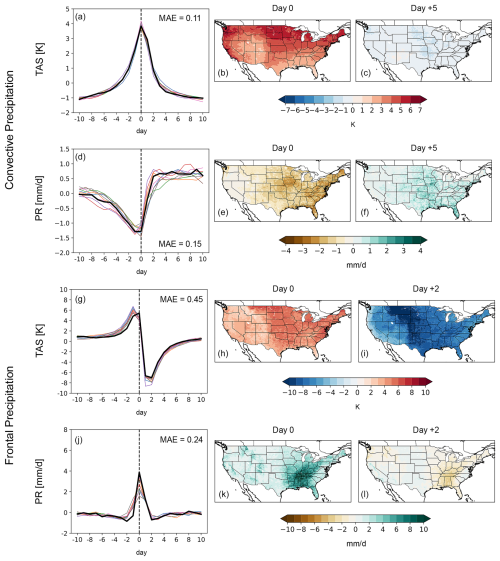
Figure 6 (a) 21 d composite (spatially averaged over the CONUS domain) time series of surface temperature anomalies (relative to the 21 d average) centered around the day of convective precipitation using LOCA2 data (colored lines; method that bias-corrects and downscales climate models) over the 1980–2014 interval. Colored lines indicate the same models as in Fig. 5. (b) Spatial composite of surface temperature on the day of convective precipitation using LOCA2. (c) Spatial composite of surface temperature 10 d prior to convective precipitation using LOCA2. (d)–(f) Same as (a)–(c) but for precipitation. (g) The 21 d composite time series (spatially averaged over CONUS domain) of surface temperature anomalies (relative to the 21 d average) centered around the day of frontal precipitation using LOCA2 data (colored lines) over the 1980–2014 interval. Colored lines indicate the same models as in Fig. 5. (h) Spatial composite of surface temperature on the day of convective precipitation using LOCA2 data. (i) Spatial composite of surface temperature anomalies 10 d prior to convective precipitation using LOCA2 data. (j)–(l) Same as (g)–(i) but for precipitation. Mean absolute error (MAE) is calculated between (i) ERA5 time series and (ii) LOCA2 time series and provided in the corners of panels (a), (d), (g), and (j).

Figure 7 Same as Fig. 6 but for STAR-ESDM data.

We next examine these same co-evolutions after the GCMs are statically downscaled using LOCA2 and STAR-ESDM techniques (Figs. 6 and 7; note that the same eight models are examined across the raw GCMs and statistically downscaled data). For temperature, differences amongst the eight GCMs (i.e., inter-model spread) are noticeably reduced for both convective and frontal precipitation (see surface temperature time series of the 21 d examined in Figs. 6 and 7). This is somewhat expected as the downscaling method bias-corrects the GCMs to “match” observations; deviations relative to observations (Livneh dataset for LOCA2 and nClimGrid-Daily dataset for STAR-ESDM) will thus be minimized. Spatial composites of downscaled surface temperature, for instance, closely mirror those shown in ERA5 for both convective and frontal precipitation. Inter-model spread for precipitation can also be reduced, though this influence is less pronounced than for temperature. Note that bias-correction during statistical downscaling is performed variable by variable (i.e., independently and without explicit consideration of local co-variances across variables) and that our definitions of convective and frontal precipitation in effect select precipitation fields based on surface temperature characteristics. Inter-model spread for downscaled precipitation fields is thus not explicitly prescribed for reduction. Our results suggest that the LOCA2 and STAR-ESDM downscaling techniques generally preserve co-variances shown in the raw GCMs with high fidelity (compare, for instance, mean absolute error values for raw GCMs against their downscaled counterparts in Figs. 5–7).

Figure 8 Same as Fig. 5 but for the 2065–2099 interval under SSP585 forcing.

There are nevertheless clear ensemble mean differences between the downscaled products and the raw GCMs (and by extension ERA5 which the raw GCMs simulate with high skill) that require careful attention. LOCA2 appears nearly identical to ERA5 for convective precipitation; however, it dampens frontal precipitation relative to ERA5 (and the raw GCMs) by up to ∼ 2 mm d⁻¹ (Figs. 5 and 6). Composite time series show LOCA2 frontal precipitation peaks at lower anomaly values (2.5 mm d⁻¹ for the LOCA2 ensemble mean verses 3.9 mm d⁻¹ in ERA5). The wet pattern apparent in the ERA5 composite is also diminished in the ensemble mean spatial composite. Importantly, such dampening is robust across most of the LOCA2 ensemble (Fig. 6), indicating it is an emergent feature of the LOCA2 downscaling method. STAR-ESDM does not exhibit this dampening: it shows frontal precipitation anomalies that closely match the frontal precipitation anomalies of ERA5 and the raw GCMs (Fig. 7j–l). STAR-ESDM may slightly overshoot drying anomalies prior to convective precipitation (by less than ∼ 0.5 K); this influence is nevertheless modest, and the STAR-ESDM ensemble simulates a range that encapsulates the evolution of frontal precipitation shown in ERA5.

3.3 Precipitation processes in raw and statistically downscaled GCMs over the future interval

We next examine convective and frontal precipitation in the raw GCMs over the future interval (2065–2099; Fig. 8). For convective precipitation, the co-evolution of surface temperature and precipitation (including the magnitude of their respective anomalies) does not change substantially across the ensemble mean relative to the historical interval (compare Figs. 5a–c to 8a–c). For frontal precipitation, however, there is robust intensification that is present across all ensemble members: frontal precipitation peaks at ∼ 4 mm d⁻¹ over the historical interval (Fig. 5e) but ∼ 5–6 mm d⁻¹ in the future interval (Fig. 8e). Scatterplots of surface temperature and peak frontal precipitation (Fig. S4) show steeper associations between the two in the future interval, indicating that frontal precipitation is driven at least in part by temperature increases. Moist static energy levels prior to frontal precipitation are also greater in the future interval relative to the historical interval (compare Figs. 5f to 8f), which is consistent with frontal precipitation intensification.

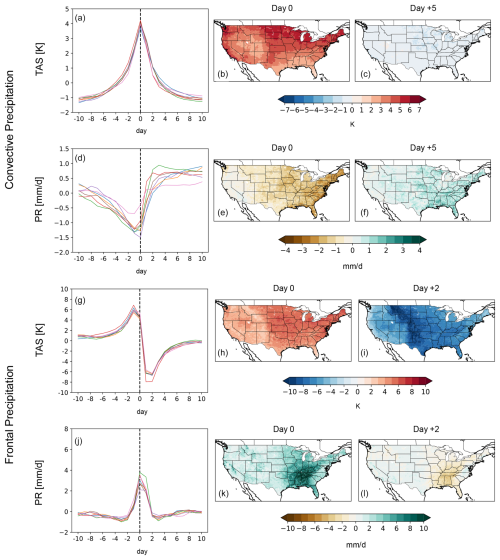
Figure 9 Same as Fig. 6 but for the 2065–2099 interval under SSP585 forcing. Colored lines indicate the same models as in Fig. 8.

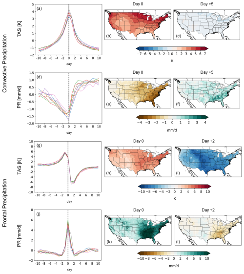
Figure 10 Same as Fig. 7 but for STAR-ESDM data. Colored lines indicate the same models as in Fig. 8.

We again examine these same co-variances after the GCMs are statically downscaled for the future interval. Future interval time series and spatial composite results for both LOCA2 and STAR-ESDM products appear nearly identical to those of the historical interval, respectively, for convective precipitation (Figs. 9a–f and 10a–f). This is consistent with expectations as the raw GCMs themselves do not show appreciable changes for convective precipitation relative to the historical interval. The robust intensification of frontal precipitation (relative to the historical interval) simulated by the raw GCMs is not evident in LOCA2 (Fig. 9g–i), some slight wetting notwithstanding. LOCA2 dampens frontal precipitation over both historical and future intervals; the net effect is that it substantially underestimates future frontal precipitation relative to the raw GCMs. For instance, frontal precipitation anomalies reach ∼ 7 mm d⁻¹ in the raw GCMs but less than 4 mm d⁻¹ in LOCA2 (and as little as 2 mm d⁻¹). Frontal precipitation is intensified in STAR-ESDM (Fig. 10j–l; ∼ 4–6 mm d⁻¹ in the future interval compared to ∼ 3–5 mm d⁻¹ in the historical interval), although the magnitude of the intensification falls short of what is simulated by the raw GCMs.

3.4 Precipitation processes in NA-CORDEX dynamical downscaling

Finally, we examine how convective and frontal precipitation processes are affected post dynamical downscaling across five different regional climate models. Dynamical downscaling of ERA-Interim preserves expected hydroclimate co-variances during convective and frontal precipitation processes (Fig. S5; note that inter-model differences are entirely attributable to regional climate models as the underlying data being downscaled is identical across the five models). Biases in regional climate models appear to be relatively small and are not prohibitive in representing convective and frontal precipitation processes at local scales. These biases are also small when GCM data, instead of observation data, are downscaled. Convective precipitation processes in dynamical downscaled GCM data in the future interval do not change much relative to the historical interval, which is consistent with the raw GCMs and with statistical downscaling (Fig. 11). However, we find that dynamical downscaling preserves robust intensification of future frontal precipitation simulated by raw GCMs in strong contrast to the dampening of this intensification seen with statistical downscaling (Fig. 12). For instance, frontal precipitation in the future interval of dynamically downscaled GCM data is ∼ 1.5 to 2 mm d⁻¹ greater than dynamically downscaled GCM data in the historical interval (Figs. S6 and 12), which is consistent with the magnitude of intensification seen with the raw GCMs. This finding is robust across all five regional climate models examined, indicating low sensitivity to regional model biases. Note that the comparison between the raw CMIP6 GCMs and downscaled CMIP5 outputs may be somewhat influenced by the specific subset of models as some CMIP6 GCMs exhibit higher climate sensitivity in comparison to CMIP5 (e.g., Meehl et al., 2020).

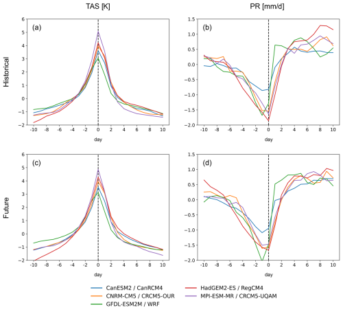
Figure 11 The 21 d composite time series of CONUS (a) surface temperature and (b) precipitation anomalies (relative to the 21 d average) centered around the day of convective precipitation using dynamical downscaling of ERA-Interim data over the 1989–2009 interval. (c)–(d) Same as (a)–(b) but for the future interval over 2065–2098 under RCP8.5 forcing.

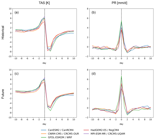
Figure 12 The 21 d composite (spatially averaged over the CONUS domain) time series of (a) surface temperature anomalies (relative to the 21 d average) and (b) precipitation anomalies (relative to the 21 d average) centered around the day of convective precipitation using NA-CORDEX dynamical downscaling of GCM data over the 1980–2014 interval. (c)–(d) Same as (a)–(b) but for the future interval over 2065–2098 under RCP8.5 forcing. Note that the years 2006–2014 fall under the RCP8.5 scenario for NA-CORDEX.

4 Conclusions

Using (only) surface temperature and precipitation outputs, we have employed convective and frontal precipitation mechanisms to evaluate the credibility of statistical (and dynamical) downscaling products. We find that the LOCA2 and STAR-ESDM statistical downscaling techniques generally preserve expected co-variances between temperature and precipitation during convective precipitation over both historical and future intervals. Statistical downscaling also preserves expected co-variances of temperature and precipitation during frontal precipitation events over the historical interval; however, it dampens projected intensification of frontal precipitation in the future interval that is otherwise robustly simulated in the raw CMIP6 GCMs (i.e., prior to downscaling) and with dynamical downscaling.

Convective precipitation in the raw GCMs as examined in our analyses does not exhibit material differences across the historical and future intervals (as opposed to frontal precipitation, which shows robust intensification in the future interval). Convective precipitation is therefore likely more insensitive to the stationarity assumption, notwithstanding the possibility that CMIP6 models themselves may not effectively resolve global cloud systems (and thus may not capture non-stationary changes in convective precipitation). Frontal precipitation, on the other hand, shows robust intensification over the future interval, providing a useful evaluation insight into the (in)ability of historical functional relationships inherent to statistical downscaling to resolve non-stationary phenomena. Indeed, the dampening of frontal precipitation shown suggests that LOCA2 and STAR-ESDM may not appropriately capture structural changes in meteorological phenomena. This is in strong contrast to dynamical downscaling (regardless of the regional climate model chosen), which preserves non-stationary physical relationships among variables.

Our results are, to some extent, qualitatively intuitive: common statistical downscaling methods apply historical functional relationships to the future under the assumption that they will be preserved despite climate change. It is therefore somewhat expected that such techniques may underestimate changes within non-stationary phenomena. This effect should be acknowledged when estimating the magnitude of future change, particularly when considering the dominant (e.g., Baek et al., 2019, 2021) and/or non-stationary (e.g., Baek et al., 2020; Scholz et al., 2022) nature of internal atmospheric variability in driving hydrologic hazards. Evaluation frameworks clearly demonstrating this to be the case have nevertheless proved elusive. Our work addresses this important gap by demonstrating divergence between statistically and dynamically downscaled methods when estimating the enhancement of frontal precipitation (an example of non-stationary process testable with just daily surface temperature and precipitation). These same issues are likely to arise among data-driven (i.e., machine learning based) climate models, particularly if those methods are only trained on historical data and subsequently used for future projections. Equally as importantly, our work highlights expected co-evolution of precipitation and temperature during convective and frontal precipitation events as process-based evaluation diagnostics that can be universally applied to a wide range of statistically downscaled products.