A revised ocean mixed layer model for better simulating the diurnal variation in ocean skin temperature

Sea surface temperature (SST) is a crucial parameter in climate, weather, and ocean sciences due to its decisive role in ocean–atmosphere interactions. Identifying errors in the prognostic scheme used by the current European Centre for Medium-range Weather Forecasts (ECMWF) model for predicting the diurnal variation in ocean skin temperature led to a revisit and revision of the ocean mixed layer (OML) model. Validation of the revised model was conducted by comparing simulated temperatures at the sub-skin level and 1 m depth with observations from shipborne infrared measurements and buoys. These comparisons revealed a strong correlation, with an absolute mean deviation of less than 0.1 K and a standard deviation under 0.5 K, which are found to be comparable to errors in satellite observations of SST. Given that these results are derived from the same model simulations, the error statistics for the simulated skin temperature and its diurnal variation should have the same degree of accuracy. Furthermore, the simulation results closely align with anticipated solar radiation distributions, whereas ERA5 ocean skin temperature shows a significant lack of alignment with solar radiation. Consequently, the revised OML model shows promising potential for improving the simulation of diurnal SST variations in weather and climate models.

1 Introduction

Sea surface temperature (SST) is recognized as an essential climate variable by the global climate observing system (Bojinski et al., 2014) and holds profound significance in climate, weather, and ocean sciences. SST influences crucial atmospheric processes such as evaporation, cloud formation, precipitation, and circulation patterns, playing a pivotal role in both short-term weather events and long-term climate phenomena (Manning and Solomon, 2007). SST's involvement in phenomena like El Niño and La Niña drives global shifts in weather patterns, underscoring its essential role in the Earth–atmosphere climate system (Lau, 1997; McPhaden et al., 2006). Additionally, SST's response to elevated CO₂ levels raises critical questions about its contribution to changes in atmospheric circulation and the global hydrological cycle (Xie et al., 2010; Burls and Fedorov, 2017; Sohn et al., 2019; Zhang et al., 2023). These implications extend to ocean studies, encompassing ocean–atmosphere interactions and associated chemical and biological processes (Chavez et al., 2002; Holmgren et al., 2006).

Current methods for constructing SST data across the global oceans, available on a daily timescale, incorporate satellite-borne radiometric measurements and buoy and shipborne measurements (Reynolds and Smith, 1994; Ishii et al., 2005; Reynolds et al., 2007; Donlon et al., 2012; Titchner and Rayner, 2014). While these measurements provide indispensable inputs for weather and climate models and diagnostic studies, they represent temperatures at certain depths (Kawai and Wada, 2007). However, numerical weather prediction (NWP) models require the temperature at the air–sea interface, referred to as the ocean skin temperature, for calculating air–sea fluxes. This is because it is the ocean skin temperature governing the thermodynamic coupling of the ocean and atmosphere (Webster and Lukas, 1992). Directly measuring this skin temperature presents challenges, so theoretical and empirical approaches are employed to estimate it using various measured SSTs as inputs (Fairall et al., 1996a).

Ocean skin temperatures vary diurnally in response to the solar cycle (Price et al., 1986). These diurnal variations, often fluctuating within a range smaller than 1 K (Fairall et al., 1996b; Ward, 2006; Wells et al., 2009), can occasionally exceed a few degrees under conditions of weak wind and strong insolation (Donlon et al., 1999; Merchant et al., 2008). Such variations play a crucial role in the heat budget. Even a 1 K error in skin temperature can lead to a substantial 27 W m⁻² error in surface net heat flux, as evidenced in the tropical western Pacific (Webster et al., 1996). Capturing this diurnal variability is essential, as skin temperature governs moisture, heat, and radiation fluxes that dictate ocean–atmosphere interactions. Consequently, accurate modeling of diurnal variation in skin temperature is important for studying heat budgets and related phenomena.

Despite the importance of ocean skin temperature, assessments of its accuracy in reanalysis products or numerical weather prediction model simulations are rare. Some studies have evaluated the performance of ocean skin temperature in ERA5 reanalysis by comparing it against SST observations from field campaigns and meteorological stations (e.g., Luo and Minnett, 2020). However, since ERA5 skin temperature and in situ observations represent different depths, results derived from direct comparisons should be interpreted with caution.

In this study, we examine the skin temperature in the ERA5 reanalysis. The European Centre for Medium-range Weather Forecasts (ECMWF) model employs an ocean prognostic scheme (Zeng and Beljaars, 2005; ECMWF, 2016) for predicting ocean skin temperature. However, as revealed in Sect. 3, this prognostic scheme contains errors, leading to concerns that the diurnal variation in the ERA5 reanalysis might be questionable. Recognizing potential issues in generating ocean skin temperatures in the ECMWF model, we scrutinize the errors in the Zeng and Beljaars (2005) scheme and attempt to revise it. We then examine the impact of the revised scheme on the diurnal variation in skin temperature and assess the accuracy of the corrected skin temperature. The results and insights gained from this study aim to improve weather forecasting and climate simulation.

2 Used data

This study involves simulating the diurnal variation in ocean skin temperature using the revised prognostic scheme and validating its simulation results. This scheme is commonly categorized as the ocean mixed layer (OML) model, as per Noh et al. (2011). Hereafter, we will refer to this prognostic scheme as the OML model. To perform the simulation, it is necessary to provide forcings associated with heat exchanges at the air–sea interface as inputs to the OML model. Although the ocean skin temperature can be simulated with a forecasting model, due to the complexity and limited availability of running such a model, we utilize ERA5 surface heat fluxes as inputs to the revised OML model. In the following subsections, we detail the input and validation data used in this study.

2.1 ERA5 hourly ocean skin temperature (T_s) and atmospheric and oceanic forcing

The ERA5 reanalysis, the fifth reanalysis project by ECMWF, provides high-resolution global atmospheric and surface data from 1940 onwards. This reanalysis is based on the forecast model of the integrated forecasting system (IFS) version Cy41r2 and the 4D-Var data assimilation system (Hersbach et al., 2020). In ERA5, the hourly ocean skin temperature (T_s) is simulated using the OML model, which is introduced in Sect. 3. The OML model accounts for interactions between the atmosphere and ocean by considering both atmospheric forcing and oceanic condition. Specifically, the oceanic condition is represented by SST, which serves as a baseline temperature for simulating the time-varying T_s in the OML model (Fig. 1). Here, SST is defined as the temperature at the depth where diurnal variation becomes less meaningful. It is updated daily at 22:00 UTC with externally supplied observation-based daily SST data (i.e., Operational Sea Surface Temperature and Ice Analysis (OSTIA) level 4 data; Donlon et al., 2012) and remains fixed until the next update cycle. Thus, ERA5 SST differs from SSTs measured by infrared (IR) instruments or buoys, which represent depths of approximately 10 µm and 1 m, respectively.

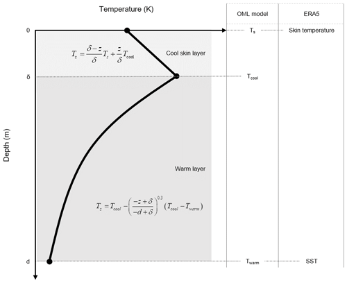
Figure 1 Schematic diagram illustrating the ocean mixed layer (OML) model. T_s, T_cool, and T_warm represent the temperatures at three levels of the OML model. In ERA5, skin temperature and SST correspond to T_s and T_warm, respectively. Temperature T_z represents the temperature at depth z. The thick solid lines depict the temperature profiles as expressed by two equations in the cool-skin and warm layers.

In this study, ERA5 single-level surface parameters are utilized. As inputs for running the revised OML model, we use net solar (shortwave) and thermal (longwave) radiation fluxes, sensible and latent heat fluxes, and 10 m neutral wind speed as atmospheric forcings and SST as the oceanic condition. All data are provided on a 0.25° × 0.25° latitude–longitude grid with an hourly resolution over the open ocean between 60° S and 60° N.

2.2 M-AERI-measured sea surface temperature at the sub-skin level

The Marine-Atmospheric Emitted Radiance Interferometer (M-AERI) is a Fourier transform IR interferometer specifically designed for deployment on ship decks. It measures temperatures using a wavelength of 7.7 µm at an incidence angle of 55° with a spectral resolution of 0.5 cm⁻¹ and a temporal resolution of 5 min. However, since IR radiation penetrates only a very thin ocean layer, the measured temperature may not be exactly the same as T_s but rather represents the temperature at about 10 µm depth (Shaw et al., 2001). Because of that, we consider M-AERI data as “sea surface temperature at the sub-skin level or sub-skin sea surface temperature”. Detailed information about the sensor and the retrieval algorithm can be found in Minnett et al. (2001).

The simulation results at sub-skin level using the OML model are validated against M-AERI measurements. The M-AERI data, spanning an 8-year period from 2013 to 2020, are collected from 24 voyages (Minnett et al., 2020). Of these, 2 voyages from 2020 are used to determine the scaling factor for parameter λ (detailed in Appendix A), while the remaining 22 voyages from 2013 to 2019 are used for model validation. Details of the individual cruises, vessels, and their tracks can be found in Fig. S1 and Table S1 in the Supplement. We select only measurements with an uncertainty range within 0.1 K (Minnett et al., 2005) and a distance of at least 25 km away from the coastline. The data are then thinned to 1 h intervals to align with the model's temporal resolution. Additionally, a spatial collocation procedure is performed, mapping data points to the nearest model grid points.

2.3 ATLAS buoy-measured sea surface temperature at 1 m depth

The simulation results at a depth of 1 m are validated against measurements from the Autonomous Temperature Line Acquisition System (ATLAS) mooring buoys, deployed within the Tropical Atmosphere Ocean (TAO) array. These buoys are equipped with 11 temperature thermistors positioned at depths ranging from 1 to 500 m, enabling temperature profiling throughout the ocean column up to 500 m depth (Milburn et al., 1996). In this study, we use temperature data collected at 1 m depth with a temporal resolution of 10 min from 54 buoys over a 20-year period from 2001 to 2020. Among these, data from a single buoy located at 0°, 140° W are used for modifying the model's stability functions (detailed in Appendix B), while the remaining 53 buoys are used for model validation. The geographical distribution of the buoys and their coordinates can be found in Fig. S1 and Table S2. We select only measurements that are continuously observed over 24 h and whose diurnal variations fall within 3 standard deviations (1.9 K) of the buoy's overall diurnal variations. The data are then thinned to 1 h intervals to match the model's temporal resolution. As all the buoys were deployed at locations coinciding with the model grid points, no additional spatial collocation procedure is necessary.

3 Revising ocean mixed layer model

In this section, we report that the OML model described in Zeng and Beljaars (2005) and ECMWF (2016), introduced to calculate the diurnal variation in T_s in the current ECMWF model, contains errors. Our goal is to correct errors and revise the OML model. The revised model will then be validated using the data described in Sect. 2.

3.1 Revised model

The OML model is designed to simulate the temperature profile and diurnal variation resulting from energy exchange and turbulent mixing processes occurring in the upper-ocean layer. The model consists of the two layers (i.e., cool-skin layer and warm layer) as described by Zeng and Beljaars (2005). Refer to Fig. 1 for a schematic diagram of the model structure and definitions of the various temperatures.

The T_s is known to be approximately 0.1–0.3 K cooler than the temperature a few millimeters below, a phenomenon known as the cool-skin effect. The thin layer influenced by this effect is referred to as the cool-skin layer (Ewing and McAlister, 1960; Saunders, 1967; Grassl, 1976), with its bottom temperature defined as T_cool. Within the cool-skin layer, the temperature varies linearly with depth. Beneath the cool-skin layer is a layer that experiences diurnal variation, called the warm layer. The warm layer is defined as the upper few meters of the ocean where solar radiation causes significant warming relative to the deep mixed layer temperature (Fairall et al., 1996b). The bottom of the warm layer is not where the diurnal variation in temperature vanishes but where this variation becomes less meaningful. Consequently, the depth of the warm layer can vary, as noted in various studies: 2–4 m (Zeng and Beljaars, 2005; ECWMF, 2016), 5–10 m (Fujiwara et al., 2017), and 1–5 m (GHRSST Science Team, 2022). In this study, we have adopted a depth of 5 m, the upper bound proposed by the GHRSST Science Team (2022), as the depth of the warm layer.

The temperature at the bottom of the warm layer (T_warm) is assumed to have no diurnal variation, representing the model's bottom boundary condition. It is updated daily with observation-based temperature and remains fixed until the next update. Note that T_warm is equivalent to ERA5 SST. Within the warm layer, the temperature profile varies in a pre-established hyperbolic function, given in Eq. (A1) of Appendix A (also given in Fig. 1). The theoretical background for the OML model was established by Saunders (1967) and Fairall et al. (1996b), with further numerical studies conducted by Fairall et al. (1996b), Beljaars (1997), and Zeng and Beljaars (2005).

However, it has been recognized that errors are present in the description of the energy balance at the air–sea interface, and it appears that these errors have been propagated to other studies without correction. In Eq. (4) of Zeng and Beljaars (2005), the temperature difference between the top and the bottom of the cool-skin layer (i.e., T_s − T_cool) is expressed as follows:

$$\begin{array}{}\text{(1)}& T_{\mathrm{s}}-T_{\mathrm{cool}}={\displaystyle \frac{\mathit{\delta }}{k_{\mathrm{w}}{\mathit{\rho }}_{\mathrm{w}}{c}_{\mathrm{w}}}}\left(H+E+\mathrm{LW}+f_{\mathrm{s}}\mathrm{SW}\right).\end{array}$$

In Eq. (1), δ (in meters) denotes the depth of the cool-skin layer. The parameters ρ_w, c_w, and k_w represent the density (kg m⁻³), specific heat capacity (J kg⁻¹ K⁻¹), and conductivity (W m⁻¹ K⁻¹) of ocean water, respectively, and H, E, LW, and SW (all in W m⁻²) are the sensible heat flux, latent heat flux, surface net longwave radiation flux, and surface net shortwave radiation flux, respectively. The dimensionless parameter f_s represents the shortwave absorptivity at the ocean surface. The energy source terms on the right-hand side, except for the shortwave flux (SW), mainly contribute to cooling the surface. We denote these terms as Q (i.e., Q = H + E + LW). The convention for vertical fluxes here is negative when going out from the surface, meaning Q is given as a negative value, while SW is given as a positive value.

In Zeng and Beljaars (2005), k_w was defined as the thermal conductivity in Eq. (1). However, if k_w is the thermal conductivity, the units on the left- and right-hand sides are not the same. The same error is found in ECMWF (2016), where k_w is set to 0.6 – see Eq. (8.151) in ECMWF (2016). In Eq. (1), k_w should be the heat diffusivity, which is on the order of 10⁻⁷. Even if we ignore the unit discrepancy, the temperature difference derived using k_w=0.6 is roughly 10³ times smaller than that obtained using correct heat diffusivity, resulting in a near-zero temperature difference between the top and bottom of the cool-skin layer.

For corrections, we first change k_w to the more common acronym h_w for thermal diffusivity and reserve k_w for thermal conductivity. The corrected version of Eq. (1) should then be

$$\begin{array}{}\text{(2)}& T_{\mathrm{s}}-T_{\mathrm{cool}}={\displaystyle \frac{\mathit{\delta }}{h_{\mathrm{w}}{\mathit{\rho }}_{\mathrm{w}}{c}_{\mathrm{w}}}}\left(Q+f_{\mathrm{s}}\mathrm{SW}\right),\end{array}$$

where k_w=h_w ⋅ ρ_w ⋅ c_w, or, if heat conductivity is used,

$$\begin{array}{}\text{(3)}& T_{\mathrm{s}}-T_{\mathrm{cool}}={\displaystyle \frac{\mathit{\delta }}{k_{\mathrm{w}}}}\left(Q+f_{\mathrm{s}}\mathrm{SW}\right).\end{array}$$

Besides the error related to the heat conductivity/diffusivity, another error is identified in the description of δ parameterization, which is given in Eq. (6) of Zeng and Beljaars (2005) as well as in Eq. (8.155) in ECMWF (2016), i.e.,

$$\begin{array}{}\text{(4)}& \mathit{\delta }=\mathrm{6}{\left\{\mathrm{1}+{\left[{\displaystyle \frac{-\mathrm{16}g{a}_{\mathrm{w}}{v}_{\mathrm{w}}^{\mathrm{3}}}{u_{\ast \mathrm{w}}^{\mathrm{4}}{k}_{\mathrm{w}}^{\mathrm{2}}{\mathit{\rho }}_{\mathrm{w}}{c}_{\mathrm{w}}}}\left(Q+f_{\mathrm{s}}\mathrm{SW}\right)\right]}^{\mathrm{3}/\mathrm{4}}\right\}}^{\mathrm{1}/\mathrm{3}},\end{array}$$

where g, ν_w, a_w, and u_∗w denote the acceleration of gravity (m s⁻²), kinematic viscosity of water (m² s⁻¹), thermal expansion coefficient of water (K⁻¹), and friction velocity of water (m s⁻¹), respectively.

In line with Eq. (2), δ should be as follows:

$$\begin{array}{}\text{(5)}& \mathit{\delta }=\mathrm{6}{\left\{\mathrm{1}+{\left[{\displaystyle \frac{-\mathrm{16}g{\mathit{\rho }}_{\mathrm{w}}{c}_{\mathrm{w}}{a}_{\mathrm{w}}{v}_{\mathrm{w}}^{\mathrm{3}}}{u_{\ast \mathrm{w}}^{\mathrm{4}}{k}_{\mathrm{w}}^{\mathrm{2}}}}\left(Q+f_{\mathrm{s}}\mathrm{SW}\right)\right]}^{\mathrm{3}/\mathrm{4}}\right\}}^{\mathrm{1}/\mathrm{3}}.\end{array}$$

However, even after correcting the conductivity/diffusivity issue, units on the left- and right-hand sides in Eq. (5) are not the same (i.e., meter ≠ unitless). It was found that Eq. (5) should not refer to the depth of the cool-skin layer (δ) but to the Saunders constant (λ, which is dimensionless and analogous to the Reynolds number; Fairall et al. 1996b). Thus, the correct expressions are

$$\begin{array}{}\text{(6)}& \mathit{\lambda }=\mathrm{6}{\left\{\mathrm{1}+{\left[{\displaystyle \frac{-\mathrm{16}g{\mathit{\rho }}_{\mathrm{w}}{c}_{\mathrm{w}}{a}_{\mathrm{w}}{v}_{\mathrm{w}}^{\mathrm{3}}}{u_{\ast \mathrm{w}}^{\mathrm{4}}{k}_{\mathrm{w}}^{\mathrm{2}}}}\left(Q+f_{\mathrm{s}}\mathrm{SW}\right)\right]}^{\mathrm{3}/\mathrm{4}}\right\}}^{\mathrm{1}/\mathrm{3}},\end{array}$$

$$\begin{array}{}\text{(7)}& \mathit{\delta }={\displaystyle \frac{v_{\mathrm{w}}}{u_{\ast \mathrm{w}}}}\mathit{\lambda }.\end{array}$$

In the OML model, the stability functions for the warm layer depend on the model configuration, such as the model integration time and the depth of the warm layer, as depicted in Eq. (A8) of Appendix A. Therefore, the current stability functions need to be rebuilt to align with the revised model configuration. In this study, new stability functions have been derived using ATLAS buoy data collected at 0°, 140° W from 2001 to 2020 (detailed in Appendix B). Furthermore, as reported in Zhang et al. (2021), adjusting the parameter λ can effectively alleviate the bias in T_s. This is because δ is proportional to λ, as shown in Eq. (7), and the T_s is proportional to δ for the given heat supply to the cool-skin layer. Similarly, we have introduced a scaling factor to adjust λ, and it has been set to 0.2 through a comparison with M-AERI data from two voyages conducted in the year 2020 (detailed in Appendix A).

With the corrections and modifications mentioned above, the implemented OML model is referred to as the “revised” OML model in this study. Correcting the erroneous equations used in the original model, which do not show even unit consistency, is only part of the revision process. Since the original model was developed based on incorrect equations, the entire simulation process was also considered flawed. Therefore, rectifying the identified errors requires a comprehensive rebuild of the model, including the development of corrected equations, model configuration, and new calculations of stability functions with the revised model. A detailed description of the model structure and configuration can be found in Appendix A and B.

3.2 Validation of the revised model

For validating the revised model, we simulate hourly T_s using the revised OML model with atmospheric forcing and SST data from ERA5. Ideally, these T_s simulations would be validated against in situ or satellite observations. However, due to the unavailability of T_s observations, we validate the revised model indirectly. Instead of using T_s observations, we compare the model-derived IR-sensor-measured equivalent temperatures and buoy-measured equivalent temperatures against M-AERI and buoy observations, respectively.

In the OML model, the temperature profile within the cool-skin layer is assumed to be linear. Thus, the IR-measured temperature, representing the temperature at about 10 µm depth, can be interpolated using T_s and T_cool (see Fig. 1). We then compare the model-derived IR equivalent temperature with the M-AERI-measured temperature from 22 voyages spanning 7 years, from 2013 to 2019. The comparison, illustrated in Fig. 2, shows statistical results of a correlation coefficient of 0.99, a mean deviation of −0.08 K, and a standard deviation of 0.49 K from a total of 32 647 data points.

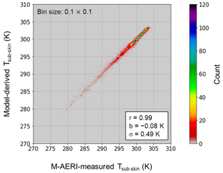
Figure 2 Scatterplot of model-derived IR equivalent temperature vs. M-AERI-measured temperature over 7 years from 2013 to 2019. The color scale is for the data count. The r, b, and σ in the inset denote correlation coefficient, mean deviation, and standard deviation, respectively.

Validation is also performed against buoy-measured temperature at a depth of 1 m. Using the pre-established shape function for the temperature profile within the warm layer (refer to Eq. A1 in Appendix A and see Fig. 1), we can estimate temperature at 1 m depth (z=1 m) by applying the shape function with T_cool and T_warm. We then compare the model-derived 1 m depth temperature against the temperatures from 53 buoys spanning the 20-year period from 2001 to 2020. The comparison results, illustrated in a scatterplot (Fig. 3), demonstrate again a good agreement with a correlation coefficient of 0.99, a mean deviation of −0.07 K, and a standard deviation of 0.28 K, based on the use of a total of 6 241 008 data points.

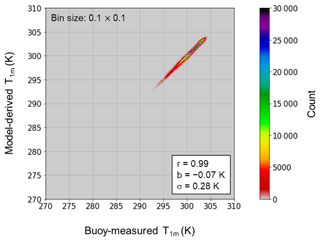
Figure 3 Same as in Fig. 2 except for model-derived 1 m depth temperature vs. buoy-measured temperature from 53 ATLAS buoys over 20 years from 2001 to 2020.

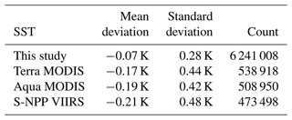
To effectively convey the significance of the error statistics in this study, we compared them with error statistics in satellite products. The model results were compared with M-AERI and 1 m depth buoy data, and existing comparisons between satellite-derived SSTs and the same observations were utilized. Error statistics for three satellite SST products based on the longwave nonlinear algorithm (Aqua MODIS, Terra MODIS, and S-NPP VIIRS) against M-AERI and buoy observations are presented in Tables 1–2, alongside the model results. It is important to note that SSTs from these three satellites are derived from IR measurements, which represent the temperature at a depth similar to the IR-based M-AERI (∼ 10 µm depth) but differ from the 1 m depth buoy-observed temperature. Consequently, IR-based satellite products show a large bias against buoy observations, which is normally corrected when buoy-like SSTs are produced from satellite measurements. From these comparisons, we conclude that the errors in model-produced temperatures at two levels are similar to those of satellite products.

Table 1 Statistics of errors in SSTs at the sub-skin layer over the global ocean: comparison of this study and satellite-sensor-retrieved temperatures vs. M-AERI-measured temperatures for best quality level only (NASA ATBD; https://oceancolor.gsfc.nasa.gov/resources/atbd/sst/#sec_4, last access: 24 July 2024).

Table 2 Same as in Table 1 except for 1 m depth buoy-measured temperature.

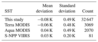
The good agreement observed in both comparisons ensures that the revised OML model can successfully reproduce hourly measured ocean temperatures within ranges suggested by the associated statistics. Therefore, although direct observational validation of T_s is not available, the high level of agreement suggests that the predicted T_s possesses a similar degree of accuracy to the estimated temperatures at 10 µm and 1 m depths. It is because these temperatures were derived from predicted T_s, T_cool, and T_warm using temperature relationships in cool-skin and warm layers.

4 Diurnal variations in T_s from ERA5 and revised model simulation

4.1 Examination of ERA5 T_s diurnal variation

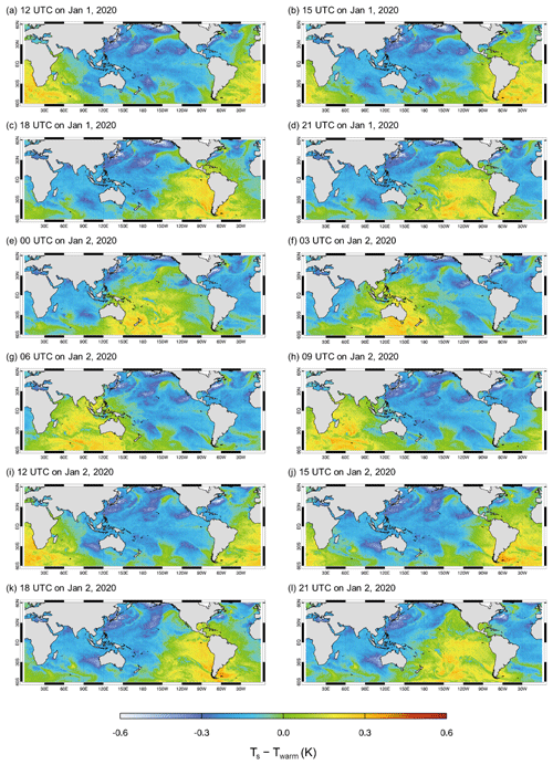
To investigate the diurnal variation in ERA5 T_s, we analyze the hourly variation in ERA5 T_s, defined as the difference between ocean skin temperature (T_s) and SST (T_warm; see Fig. 1). The ERA5 T_s is believed to be inaccurately simulated due to flaws in the OML model used by ECMWF. Figure 4 shows the geographical distribution of T_s hourly variation, given in a 3 h interval, over a period of 1.5 d (from 12:00 UTC on 1 January 2020 to 21:00 UTC on 2 January 2020). This figure visually represents the hourly variations in T_s over the global ocean, revealing significant spatiotemporal fluctuation between two specific time zones (10:00–21:00 UTC and 22:00–09:00 UTC). The fluctuations are depicted for 12:00–21:00 UTC (Fig. 4a–d), 00:00–09:00 UTC (Fig. 4e–h), and 12:00–21:00 UTC on the following day (Fig. 4i–l). Specifically, the hourly variations in Fig. 4e–h exhibit patterns with spatially incoherent, localized variations in contrast to the smoother features observed during the earlier and later 12 h periods (Fig. 4a–d and 4i–l) across the global ocean.

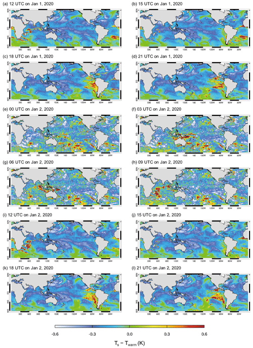
Figure 4 Geographical distributions of hourly variations in ERA5 T_s from 12:00 UTC on 1 January to 21:00 UTC on 2 January in 2020 with a 3 h interval. Values are given in departures of ERA5 ocean skin temperature from ERA5 SST (i.e., T_s–T_warm).

To illustrate the changes in T_s variation more clearly at specific times, we compare the hourly variations between 09:00 and 10:00 UTC and between 21:00 and 22:00 UTC on 1 January 2020. These times are identified as showing a spatial “disruption” in the hourly variation pattern (Fig. 5). At 09:00 UTC, the patterns appear scattered and on a much smaller scale. However, by 10:00 UTC, the patterns become significantly smoother and on a larger scale compared to the previous hour. For example, in the 30–60° S latitudinal band, scattered patterns over the southern Indian Ocean, central South Pacific, and east of New Zealand become much smoother, with localized areas of high variation disappearing. Moreover, after 12 h, between 21:00 and 22:00 UTC, the changes reverse. The patterns become scattered again, and localized areas of high variation return at 22:00 UTC, resembling the spatial patterns observed at 09:00 UTC. This indicates a cyclical disruption and smoothing pattern in T_s variation within these specific time frames.

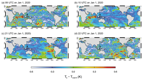
Figure 5 Same as Fig. 4 but given in hourly departures at (a) 09:00 UTC, (b) 10:00 UTC, (c) 21:00 UTC, and (d) 22:00 UTC on 1 January 2020.

The pattern transition at 09:00 and 22:00 UTC can be quantitatively assessed using the pattern correlation coefficient between two consecutive hourly T_s distributions. This coefficient provides an index of the similarity or difference between the two maps, based on the notion that temperature variations should not change abruptly within 1 h. The pattern correlation coefficient is calculated using consecutive hourly T_s distributions over the global ocean from 1 to 5 January 2020. The resulting time series is presented in Fig. 6. The time series indicates that the coefficient, which remains above 0.97, suddenly drops to approximately 0.8 at 09:00–10:00 UTC and 21:00–22:00 UTC. This abrupt and significant drop indicates a notable change in the spatial pattern at 10:00 and 22:00 UTC, while a similar pattern is maintained over the following 12 h once the pattern changed.

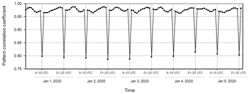
Figure 6 Time series of the pattern correlation coefficient for ERA5 T_s variations over the global ocean between two consecutive hourly distributions (between n and n+1 hourly data, expressed as $n-(n+\mathrm{1}$) UTC), in the period from 1 to 5 January 2020. Only 09:00–10:00 UTC and 21:00–22:00 UTC are given as labels.

The “abrupt” changes occurring at 10:00 and 22:00 UTC, with 12 h intervals, are far from reasonable. These abrupt changes, observed consistently at 12 h intervals, are persistent in ERA5 data. This conclusion is based on an analysis of randomly chosen 1.5 d periods each month over 20 years from 2001 to 2020, all showing the same abnormal behaviors (not shown). Furthermore, because these hourly variations contribute to the diurnal variation, which should be highly correlated with solar radiation, the abrupt changes at 09:00 and 21:00 UTC are particularly irrational. These findings raise concerns about the underlying procedures used to produce T_s in ERA5.

4.2 Examination of simulated T_s diurnal variation

To determine whether the abnormal features found in ERA5 T_s exist in our simulations, we present the hourly variations in simulated T_s in Fig. 7 using 3 h intervals over the same period as in Fig. 5. Additionally, an animation depicting the hourly variation in T_s from 1 to 5 January 2020 has been uploaded as the Supplement. It is clear that the temporal disruptions observed in ERA5 at 10:00 and 22:00 UTC are not present in our simulations. The variations between these two time zones appear continuous and smooth without disruption. Furthermore, the spatially variable and localized patterns as in ERA5 from 22:00 to 09:00 UTC (Fig. 7e–h) do not appear in the simulations.

Figure 7 Same as in Fig. 4 but for T_s simulated with the revised OML model.

Thus, it is presumed that the diurnal variations in ERA5 T_s are problematic, as the presence of alternating regimes every 12 h is not reasonable. There are no identifiable forcings that would cause periodic oscillations in the T_s variation distribution over the global ocean with a 12 h cycle. In contrast, our simulation shows high-magnitude-variation areas continuously moving westward and circulating globally, presumably following a 24 h cycle coinciding with solar forcing.

4.3 Correlation between simulated T_s and solar radiation

Given that solar radiation is a major driving force for T_s variations during the daytime, there should be a strong correlation between T_s and solar radiation during the day. Thus, a comparison of T_s with the surface net solar radiation flux can serve as another means to evaluate the model performance. Figure 8 illustrates the geographical distributions of T_s departures from T_warm for our simulation and ERA5 at 00:00 and 12:00 UTC on 2 January 2020, alongside the ERA5 surface net solar radiation flux.

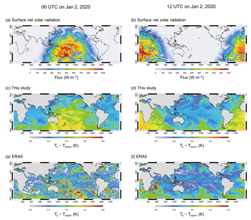
Figure 8 Geographical distributions of (a–b) surface net solar radiation flux from ERA5 and T_s hourly variations from (c–d) the revised OML model and (e–f) ERA5 at 00:00 UTC (left panels) and 12:00 UTC (right panels) on 2 January 2020.

The comparison (Fig. 8a vs. 8c and Fig. 8b vs. 8d) clearly shows that high-solar-radiation areas centered at 180 and 0° correlate well with the positive T_s departure areas. Nighttime areas exhibit small negative departures, consistent with the expectation that T_s variation is minimal during the night (Gentemann et al., 2003). In contrast, ERA5 at 00:00 UTC (Fig. 8a vs. 8e) shows no clear correspondence to solar radiation over the Pacific Ocean and lacks a distinct day-and-night contrast. Interestingly, the nighttime distribution over the Pacific Ocean at 12:00 UTC is similar to that in our simulation (Fig. 8d vs. 8f), differing from the features noted 12 h earlier (at 00:00 UTC). These results suggest that ERA5 T_s variation is not coherently modulated by surface net solar radiation, at least during the 12 h period from 22:00 to 09:00 UTC.

Furthermore, we compare the time series of T_s between this study and ERA5 for the week of 1–7 January 2020 at four locations (20° S, 80° E; 20° N, 180°; 0°, 155° W; and 30° S, 120° W) in Fig. 9. The time series of surface net solar radiation flux over the same period is also presented. It is clear that the revised OML model produces T_s variations that correlate well with solar radiation. In contrast, the ERA5 time series shows no clear correlation with solar radiation, and ERA5 T_s values consistently exhibit lower temperatures than those obtained from our simulations. These characteristics appear to extend beyond this specific analysis period. A comprehensive examination of the entire year 2020 at 0°, 155° W reveals that these traits persist throughout all seasons (Fig. S2), indicating that ERA5 daily mean values are predominantly lower than those indicated by simulations. Seasonally, ERA5 shows temperatures 0.13–0.15 K cooler than the simulations at this equatorial Pacific location.

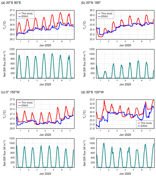
Figure 9 Time series of T_s from the model simulations and ERA5 (top subpanel of each panel) and ERA5 surface net solar radiation flux (bottom subpanel of each panel) for a period of a week from 1 to 7 January 2020 at four locations: (a) 20° S, 80° E; (b) 20° N, 180°; (c) 0°, 155° W; and (d) 30° S, 120° W.

5 Conclusions and discussion

Motivated by errors noted in the OML model used for predicting T_s in ERA5, we revisited and revised the OML model. After identifying and correcting errors in the literature describing the OML model and revising other necessary procedures, we validated the model-simulated temperature profiles in the upper-ocean boundary layer. This validation was done against observations from shipboard IR interferometers and buoy-mounted thermistors, representing temperatures at 10 µm and 1 m depths, respectively. The comparison demonstrated good agreement, with an absolute mean deviation smaller than 0.1 K and a standard deviation below 0.5 K, which are found to be comparable to error statistics for satellite measurements of SST. Since these statistical results are from simulated T_s, T_cool, and T_warm, the simulated T_s in this study would be comparable to satellite measurements if such satellite data were available. Additionally, the revised OML model indicates a strong correlation between the diurnal variations in simulated T_s and solar radiation in both geographical distributions and time series.

Given that the revised OML model employs the same underlying physics as the ERA5 OML model and that the simulations used identical inputs as ERA5, we anticipated a high degree of similarity between the two T_s datasets if the current ERA5 OML model is correct. However, the diurnal variations in ERA5 T_s deviate significantly from scientifically sound expectations when compared against model-simulated T_s and surface net solar radiation flux. In particular, ERA5 T_s shows little correlation with solar radiation despite solar radiation being a major driving force for SST variations during the daytime. These discrepancies persist throughout the year 2020, suggesting that the results are not coincidental. In addition to the unreasonable features, such as the 12 h alternating spatial patterns found in ERA5, the daily averages are substantially cooler than our simulations, and the disorganized relationship with solar radiation inevitably leads to the conclusion that ERA5 may not accurately represent the nature of diurnal variations in T_s.

The unreasonable features noted in ERA5 T_s may be attributed to the failure to simulate the temperature within the cool-skin layer due to the incorrect equation and the wrong assignment of diffusivity. In addition to the unit inconsistency, the wrong diffusivity value (i.e., 0.6 instead of $\mathrm{1.40}\times {\mathrm{10}}^{-\mathrm{7}}$ m² s⁻¹) may result in T_s being nearly equal to T_cool (i.e., T_s≈T_cool). However, in reality, as expressed in Eq. (2), T_s variation should be much larger than T_cool during the daytime due to incoming solar flux. Such an expected difference is confirmed by observing that ERA5 T_s is not very responsive to solar radiation flux (Fig. 9). Since the diurnal variation in T_cool should be smaller than T_s in accurate simulations, the diurnal variation in the current ERA5 T_s should be smaller than the new ones, as revealed in Fig. 9. Furthermore, the ERA5 T_s diurnal variation may not follow the solar flux variation, whose direct influence is on T_s. Because the cool-layer physics was effectively suppressed in the ECMWF model (as shown in T_s≈T_cool), the ERA5 T_s variation may follow the variation in the warm layer, which is more complex due to the competing influences of solar radiation and turbulent mixing. This might result in more irregular patterns, as shown in Fig. 9. It appears that the problems in the current ECMWF model may not be confined to the assignment of incorrect values for the heat diffusivity but also may reside in the warm-layer temperature variation. It is because the warm-layer process might have been developed based on incorrect equations of the cool-skin process.

In contrast, the revised OML model is capable of producing T_s diurnal variations comparable to observations and thus holds the potential to be a valuable tool for generating accurate T_s diurnal variations. The enhanced forecasting capability of the diurnal cycle of T_s, whose accuracy is comparable to satellite observations, should be beneficial across a wide range of meteorological applications and further contribute to related climate and weather studies. Since the diurnal cycle of T_s affects various factors such as surface net heat flux, surface wind, evaporation rate, and atmospheric stability, this simulation of T_s would improve weather forecasting accuracy. However, these expectations need to be confirmed through NWP model experiments using the revised OML model to examine how the improved T_s influences predicted variables. Therefore, future studies should focus on conducting NWP experiments to understand the potential benefits and limitations of the revised OML model in meteorological applications.

Appendix A

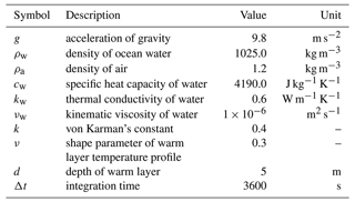
In this study, the OML model was revised by examining the theoretical development made by Fairall et al. (1996b) and Zeng and Beljaars (2005). Some errors noted in Zeng and Beljaars (2005) were corrected as described in the main text. During the model revision, stability functions for the warm layer were updated, and the scaling factor for the Saunders constant was introduced. The required input parameters to the model are the surface net solar radiation flux (SW), surface net thermal radiation flux (LW), latent heat flux (E), sensible heat flux (H), neutral wind speed at 10 m height (u_10m) as the atmospheric forcings, and SST (T_warm) as the oceanic condition. The OML model also incorporates the prescribed state parameters summarized in Table A1.

The shape function of the temperature profile within the warm layer is expressed as follows:

$$\begin{array}{}\text{(A1)}& T_z=T_{\mathrm{cool}}-{\left({\displaystyle \frac{-z+\mathit{\delta }}{-d+\mathit{\delta }}}\right)}^{\mathit{\upsilon }}\left(T_{\mathrm{cool}}-T_{\mathrm{warm}}\right),\end{array}$$

where z is the depth, ν is the shape parameter of the warm-layer temperature profile, and δ and d (both in meters) denote depths of cool-skin and warm layers. Thus, within a 1-D column, the warm layer vertically extends from δ to d, and T_cool, T_z, and T_warm (all in K) refer to the temperatures at depths of δ, z, and d, respectively.

The thermal expansion coefficient of water (α_w in K⁻¹) is parameterized as follows (ECMWF, 2016):

$$\begin{array}{}\text{(A2)}& a_{\mathrm{w}}={\mathrm{10}}^{-\mathrm{4}}\cdot max\left[T_{\mathrm{warm}}-\mathrm{273},\mathrm{1}\right].\end{array}$$

The friction velocity in the air (u_∗a in m s⁻¹) is derived from u_10 m using Eq. (A3), as introduced by Andreas et al. (2012).

$$\begin{array}{}\text{(A3)}& \begin{array}{rl}& u_{\ast \mathrm{a}}=\mathrm{0.239}+\mathrm{0.0433}\\ & \left[u_{\mathrm{10}\mathrm{m}}-\mathrm{8.271}+\sqrt{\mathrm{0.12}{\left(u_{\mathrm{10}\mathrm{m}}-\mathrm{8.271}\right)}^{\mathrm{2}}+\mathrm{0.181}}\right]\end{array}\end{array}$$

Subsequently, the friction velocity in water (u_∗w in m s⁻¹) is calculated as follows:

$$\begin{array}{}\text{(A4)}& u_{\ast \mathrm{w}}=u_{\ast \mathrm{a}}\sqrt{{\displaystyle \frac{{\mathit{\rho }}_{\mathrm{a}}}{{\mathit{\rho }}_{\mathrm{w}}}}}.\end{array}$$

We define Q = H + E + LW because of their cooling effects. It is noted that the convention for vertical fluxes is established as positive when directed into the surface and negative when directed away from the surface.

Equation (A5) describes how T_cool evolves over time:

$$\begin{array}{}\text{(A5)}& {\displaystyle \frac{\partial \mathrm{\Delta }T}{\partial t}}={\displaystyle \frac{\mathit{\alpha }}{d-\mathit{\delta }}}\left[Q+f_{\mathrm{d}}\mathrm{SW}\right]-{\displaystyle \frac{\mathit{\beta }}{d-\mathit{\delta }}}{\displaystyle \frac{u_{\ast \mathrm{w}}}{\mathit{\varphi }}}\mathrm{\Delta }T,\end{array}$$

where ΔT is the difference between T_cool and T_warm (i.e., T_cool–T_warm), and t is time. Here, d is 5 m and δ is a few millimeters, with d≫δ. Therefore, we approximate d–δ≈d in the subsequent calculations. The bulk coefficients α (in K m³ J⁻¹) and β (dimensionless) are defined as follows:

$$\begin{array}{}\text{(A6)}& \mathit{\alpha }={\displaystyle \frac{\mathit{\nu }+\mathrm{1}}{\mathit{\nu }{c}_{\mathrm{w}}{\mathit{\rho }}_{\mathrm{w}}}},\end{array}$$

$$\begin{array}{}\text{(A7)}& \mathit{\beta }=k\left(\mathit{\nu }+\mathrm{1}\right).\end{array}$$

In Eq. (A5), the first term on the right-hand side represents the heat flux from energy exchange with the atmosphere, while the second term on the right-hand side is for the ocean internal heat transport due to the turbulent diffusion.

Table A1 Symbols, descriptions, values, and units of prescribed parameters used in the revised OML model.

The numerical solution for Eq. (A5) can be obtained as follows:

$$\begin{array}{}\text{(A8)}& \begin{array}{rl}{T}_{\mathrm{cool}}^{(n+\mathrm{1})}& =T_{\mathrm{warm}}^{\left(n\right)}+{\displaystyle \frac{\mathrm{\Delta }t}{d}}\left\{\mathit{\alpha }\left[Q^{\left(n\right)}+f_{\mathrm{d}}{\mathrm{SW}}^{\left(n\right)}\right]\right.\\ & \left.-\mathit{\beta }{\displaystyle \frac{u_{\ast \mathrm{w}}^{\left(n\right)}}{{\mathit{\varphi }}^{\left(n\right)}}}\left(T_{\mathrm{cool}}^{\left(n\right)}-T_{\mathrm{warm}}^{\left(n\right)}\right)\right\},\end{array}\end{array}$$

where the superscripts n and n+1 indicate the nth and nth+1 time step. As T_warm is fixed in time, T_cool at the nth+1 time step can be determined by explicitly considering the variation induced by atmospheric forcing and vertical temperature deviation at the nth time step.

The shortwave absorptivity in the warm layer (f_d, dimensionless) is defined in Eq. (A9), with the group coefficients [A] and [B] that are defined as [A₁, A₂, A₃] = [0.28, 0.27, 0.45] and [B₁, B₂, B₃] = [71.5, 2.8, 0.07].

$$\begin{array}{}\text{(A9)}& f_{\mathrm{d}}=\mathrm{1}-\sum _{i=\mathrm{1}}^{\mathrm{3}}{A}_i{e}^{-d\cdot B_i}\end{array}$$

The stability functions (ϕ, dimensionless) of the warm layer are defined by Eqs. (A10), (A11), and (A15), which are functions of stability parameter ζ ($=d/L$). Here, we introduce new empirical ϕ–ζ relations specific to the revised model configuration (detailed in Appendix B).

$$\begin{array}{}\text{(A10)}& {\displaystyle }\mathit{\varphi }=\mathrm{2}+\mathrm{12}{\mathit{\zeta }}^{-\mathrm{0.5}}(\mathit{\zeta }>\mathrm{0})\text{(A11)}& {\displaystyle }\mathit{\varphi }=\mathrm{2}+\mathrm{8}{\left(-\mathit{\zeta }\right)}^{-\mathrm{0.5}}(\mathit{\zeta }\le \mathrm{0})\end{array}$$

Here, L (in meters) represents the Obukhov length, which is positive (negative) for stable (unstable) stratification, and it is given as follows:

$$\begin{array}{}\text{(A12)}& L={\displaystyle \frac{u_{\ast \mathrm{w}}^{\mathrm{3}}}{k{F}_{\mathrm{d}}}},\end{array}$$

where F_d is the buoyancy flux (in m² s⁻³) and is given by

$$\begin{array}{}\text{(A13)}& F_{\mathrm{d}}={\displaystyle \frac{g{\mathit{\alpha }}_{\mathrm{w}}}{{\mathit{\rho }}_{\mathrm{w}}{c}_{\mathrm{w}}}}\left(Q+f_{\mathrm{d}}\mathrm{SW}\right).\end{array}$$

In addition, to account for the phenomena of relatively warmer temperature persisting for a certain duration after sunset, when T_cool is warmer than T_warm (i.e., T_cool–T_warm≥0) and simultaneously the net flux is negative (i.e., Q + f_d SW < 0), the numerical solution for T_cool is replaced as follows:

$$\begin{array}{}\text{(A14)}& T_{\mathrm{cool}}^{(n+\mathrm{1})}=T_{\mathrm{warm}}^{\left(n\right)}+{\displaystyle \frac{\mathrm{\Delta }t}{d}}\left[-\mathit{\beta }{\displaystyle \frac{u_{\ast \mathrm{w}}^{\left(n\right)}}{{\mathit{\varphi }}^{\left(n\right)}}}\left(T_{\mathrm{cool}}^{\left(n\right)}-T_{\mathrm{warm}}^{\left(n\right)}\right)\right].\end{array}$$

For the case of sunset duration, the associated stability function and buoyancy flux within the warm layer are separately defined as follows:

$$\begin{array}{}\text{(A15)}& \mathit{\varphi }=\mathrm{2}+\mathrm{4}{\mathit{\zeta }}^{-\mathrm{1}},\end{array}$$

$$\begin{array}{}\text{(A16)}& F_{\mathrm{d}}=u_{\ast \mathrm{w}}^{\mathrm{2}}\sqrt{{\displaystyle \frac{vg{\mathit{\alpha }}_{\mathrm{w}}}{\mathrm{5}\mathrm{d}}}\left(T_{\mathrm{cool}}-T_{\mathrm{warm}}\right)}.\end{array}$$

At this point, T_cool at the nth+1 time step becomes obtainable. Moreover, if necessary, the temperature at a depth of z within the warm layer, T_z, can be determined using Eq. (A1) from T_cool and T_warm at the nth+1 time step.

The boundary condition at the air–sea interface satisfies the energy equilibrium, which is expressed as follows:

$$\begin{array}{}\text{(A17)}& k_{\mathrm{w}}{\displaystyle \frac{\partial T}{\partial z}}=Q+f_{\mathrm{s}}\mathrm{SW}.\end{array}$$

The numerical solution for T_s (in K) at the nth+1 time step is defined based on the implicit approach:

$$\begin{array}{}\text{(A18)}& T_{\mathrm{s}}^{(n+\mathrm{1})}=T_{\mathrm{cool}}^{(n+\mathrm{1})}+{\displaystyle \frac{{\mathit{\delta }}^{\left(n\right)}}{k_{\mathrm{w}}}}\left(Q^{\left(n\right)}+f_{\mathrm{s}}^{\left(n\right)}{\mathrm{SW}}^{\left(n\right)}\right),\end{array}$$

where f_s (dimensionless) is the shortwave absorptivity of the ocean surface,

$$\begin{array}{}\text{(A19)}& f_{\mathrm{s}}=\mathrm{0.065}+\mathrm{11}\mathit{\delta }-{\displaystyle \frac{\mathrm{6.6}\times {\mathrm{10}}^{-\mathrm{5}}}{\mathit{\delta }}}\left(\mathrm{1}-e^{-\mathit{\delta }/(\mathrm{8}\times {\mathrm{10}}^{-\mathrm{4}})}\right),\end{array}$$

and the depth of the cool-skin layer (δ) is defined as

$$\begin{array}{}\text{(A20)}& \mathit{\delta }={\displaystyle \frac{v_{\mathrm{w}}}{u_{\ast \mathrm{w}}}}\mathit{\lambda }.\end{array}$$

In Eq. (A20), λ (dimensionless) denotes the Saunders constant as below:

$$\begin{array}{}\text{(A21)}& \mathit{\lambda }=\mathrm{6}{\left\{\mathrm{1}+{\left[{\displaystyle \frac{-\mathrm{16}g{\mathit{\rho }}_{\mathrm{w}}{c}_{\mathrm{w}}{a}_{\mathrm{w}}{v}_{\mathrm{w}}^{\mathrm{3}}}{u_{\mathrm{w}}^{\mathrm{4}}{k}_{\mathrm{w}}^{\mathrm{2}}}}\left(Q+f_{\mathrm{s}}\mathrm{SW}\right)\right]}^{\mathrm{3}/\mathrm{4}}\right\}}^{-\mathrm{1}/\mathrm{3}}.\end{array}$$

It should be noted that Eqs. (A19) and (A21) are interdependent, i.e., f_s=f(λ) and λ=f (f_s). Thus, to obtain the numerical solutions for both variables, an iterative minimum residual approach is needed. Fairall et al. (1996b) proposed a slightly different parameterization for λ, i.e.,

$$\begin{array}{}\text{(A22)}& \mathit{\lambda }=\mathrm{6}{\left[\mathrm{1}+{\left({\displaystyle \frac{-\mathrm{16}g{\mathit{\rho }}_{\mathrm{w}}{c}_{\mathrm{w}}{a}_{\mathrm{w}}{v}_{\mathrm{w}}^{\mathrm{3}}}{u_{\mathrm{w}}^{\mathrm{4}}{k}_{\mathrm{w}}^{\mathrm{2}}}}Q\right)}^{\mathrm{3}/\mathrm{4}}\right]}^{-\mathrm{1}/\mathrm{3}}.\end{array}$$

Given that the discrepancy between Eqs. (A21) and (A22) emerges at the nanometer scale at the depth δ, the difference can be regarded as negligible. In this study, Eq. (A22) was chosen for λ.

The Saunders constant λ, analogous to the Reynolds number, plays a crucial role in simulating T_s by determining the depth of the cool-skin layer, δ. Zhang et al. (2021) reported that the bias of T_s can be effectively mitigated by adjusting λ. Similarly, we introduced a scaling factor to adjust λ, and it is set to 0.2, determined from the comparison with M-AERI data from the year 2020. This scaling factor yielded a reduction in bias from −0.38 to −0.12, and the resulting scatterplot of applying it to the 2020 data is presented in Fig. S3. As noted by Saunders et al. (1967), the magnitude of λ is in a zeroth order, implying the presence of laminar flow within the cool-skin layer. The scaled λ still falls within the magnitude of the same zeroth order, thereby retaining its laminar flow characteristics.

Appendix B

The stability functions (ϕ; Eqs. A10, A11, and A15) are formulated using data from ATLAS buoys deployed at 0° and 140° W from 2001 to 2020. These buoys measure temperatures at a depth of 1 m. Based on the relation obtained by directly comparing OSTIA data (i.e., ERA5 SST) with buoy data, their mean temperature is treated as T_warm with a non-diurnal cycle. ERA5 atmospheric forcing data are also collected. By applying the predefined temperature profile shape function (Eq. A1), T_cool can be derived from the T_1m and T_warm values. This process enables the T_cool and T_warm dataset to be organized into a specific time interval (Δt=3600 s) as n, n+1, n+2, and so forth.

The magnitude of ϕ is calculated under the two conditions proposed by Zeng and Beljaars (2005). The first condition (Case 1) is when relatively higher temperatures persist for a certain period after sunset (i.e., T_cool − T_warm ≥ 0 and Q + f_d SW < 0). The second condition (Case 2) covers all other scenarios.

$$\begin{array}{}\text{(B1)}& \mathrm{Case}\mathrm{1}:{\mathit{\varphi }}^{\left(n\right)}=\left|{\displaystyle \frac{\mathit{\beta }{u}_{\ast \mathrm{w}}^{\left(n\right)}\mathrm{\Delta }t\left(T_{\mathrm{cool}}^{\left(n\right)}-T_{\mathrm{warm}}^{\left(n\right)}\right)}{d\left(T_{\mathrm{cool}}^{(n+\mathrm{1})}-T_{\mathrm{warm}}^{\left(n\right)}\right)}}\right|\end{array}$$

$$\begin{array}{}\text{(B2)}& \begin{array}{rl}& \mathrm{Case}\mathrm{2}:{\mathit{\varphi }}^{\left(n\right)}=\\ & \left|-{\displaystyle \frac{\mathit{\beta }{u}_{\ast \mathrm{w}}^{\left(n\right)}\mathrm{\Delta }t\left(T_{\mathrm{cool}}^{\left(n\right)}-T_{\mathrm{warm}}^{\left(n\right)}\right)}{d\left(T_{\mathrm{cool}}^{(n+\mathrm{1})}-T_{\mathrm{warm}}^{\left(n\right)}\right)-\mathrm{\Delta }t\mathit{\alpha }\left(Q^{\left(n\right)}+f_{\mathrm{d}}{\mathrm{SW}}^{\left(n\right)}\right)}}\right|\end{array}\end{array}$$

The corresponding stability parameters (ζ) are calculated using Eq. (A12). The scatterplots of buoy-derived ζ vs. ϕ are presented in Fig. B1, demonstrating relationships similar to those proposed by Stiperski and Calaf (2023). As a result, the fitted ϕ–ζ relationship is determined for three distinct cases: Case 1 (for Eq. A15) and Case 2, which is further divided into ζ>0 (for Eq. A10) and ζ≤0 (for Eq. A11).

Figure B1 Scatterplots of stability functions (ϕ) vs. stability parameters (ζ), derived from ATLAS buoy measurements at 0° and 140° W in the period from 2001 to 2020: (a) Eq. (A10), (b) Eq. (A11), and (c) Eq. (A15). The color scale is for the data count, and the obtained ϕ–ζ relations are given with solid black lines.