GEO4PALM v1.1: an open-source geospatial data processing toolkit for the PALM model system

A geospatial data processing tool, GEO4PALM, has been developed to generate geospatial static input for the Parallelized Large-Eddy Simulation (PALM) model system. PALM is a community-driven large-eddy simulation model for atmospheric and environmental research. Throughout PALM's 20-year development, research interests have been increasing in its application to realistic conditions, especially for urban areas. For such applications, geospatial static input is essential. Although abundant geospatial data are accessible worldwide, geospatial data availability and quality are highly variable and inconsistent. Currently, the geospatial static input generation tools in the PALM community heavily rely on users for data acquisition and pre-processing. New PALM users face large obstacles, including significant time commitments, to gain the knowledge needed to be able to pre-process geospatial data for PALM. Expertise beyond atmospheric and environmental research is frequently needed to understand the data sets required by PALM. Here, we present GEO4PALM, which is a free and open-source tool. GEO4PALM helps users generate PALM static input files with a simple, homogenised, and standardised process. GEO4PALM is compatible with geospatial data obtained from any source, provided that the data sets comply with standard geo-information formats. Users can either provide existing geospatial data sets or use the embedded data interfaces to download geo-information data from free online sources for any global geographic area of interest. All online data sets incorporated in GEO4PALM are globally available, with several data sets having the finest resolution of 1 m. In addition, GEO4PALM provides a graphical user interface (GUI) for PALM domain configuration and visualisation. Two application examples demonstrate successful PALM simulations driven by geospatial input generated by GEO4PALM using different geospatial data sources for Berlin, Germany, and Ōtautahi / Christchurch, New Zealand. GEO4PALM provides an easy and efficient way for PALM users to configure and conduct PALM simulations for applications and investigations such as urban heat island effects, air pollution dispersion, renewable energy resourcing, and weather-related hazard forecasting. The wide applicability of GEO4PALM makes PALM more accessible to a wider user base in the scientific community.

1 Introduction

The Parallelized Large-Eddy Simulation (PALM) model is a large-eddy simulation (LES) model that has been used for atmospheric boundary layer (ABL) research for over 20 years (Maronga et al., 2015, 2020; Raasch and Schröter, 2001). PALM is a free and open-source model with high scalability to simulate atmospheric flows from the mesoscale (10 to 200 km) to the microscale (1 cm to 1 km). To resolve land surface physics, PALM provides several features including the radiative transfer model (RTM; Krč et al., 2021), land surface model (LSM; Gehrke et al., 2021), urban surface model (USM; Resler et al., 2017), and plant canopy model (PCM; Maronga et al., 2020). Over the last few years, PALM has been extensively developed for various microscale and mesoscale applications, especially for wind energy and urban applications. With the implementation of new modules, PALM has been used to study wind turbine wake in a German wind farm (Vollmer et al., 2017) and urban environments, such as ventilation in the city of Hong Kong (Gronemeier et al., 2017) and urban air quality and pollutant dispersion in Cambridge, the United Kingdom (Kurppa et al., 2019); Helsinki, Finland (Kurppa et al., 2020); and Bergen, Norway (Wolf et al., 2020, 2021). In addition, several studies (e.g. Belda et al., 2021; Resler et al., 2021; Salim et al., 2022) have carried out sensitivity analysis and simulations to validate PALM in urban environments. Geospatial data sets that describe the land surface characteristics and provide ground surface boundary conditions to the atmospheric model are critical for realistic simulations, especially for microscale and/or urban climate studies.

The exchanges of energy and moisture between the surface and the atmosphere are impacted by physical characteristics of the land surface, such as urban canopy, plant canopy, topography, and land use, across a spectrum of spatial and temporal scales throughout the atmospheric boundary layer (ABL; e.g. Bou-Zeid et al., 2004; Maronga et al., 2014; Rihani et al., 2015; Srivastava et al., 2020). To include, resolve, and realise the near-surface physical characteristics, PALM’s current initialisation setup allows users to provide a NetCDF static driver strictly formatted in PALM Input Data Standard (PIDS) as an input (hereafter referred to as the static driver). In PALM, geospatial data should be processed and stored in a static driver to carry out simulations. Heldens et al. (2020) described the data requirements of the static driver for PALM and provided the PALM Create Static Driver tool (hereafter PALM CSD) to generate a static driver for PALM using geospatial data. However, the data processing routine provided by Heldens et al. (2020) is heavily dependent on the geospatial data set prepared by the German Space Agency (DLR), for example, for three cities in Germany (Stuttgart, Berlin, and Hamburg) described in their study. The PALM CSD tool can only process data in NetCDF format with its particular data standard, which requires users to dedicate significant time to pre-processing the geospatial data.

In addition to PALM CSD, palmpy (https://github.com/stefanfluck/palmpy, last access: 29 January 2024; Fluck, 2020) is another tool developed to generate static driver input for PALM applications at the Centre for Aviation (ZAV), Zurich University of Applied Sciences, Switzerland (Liu et al., 2022). The palmpy tool is more generally applicable compared to PALM CSD, but, to the best of our knowledge, it has mainly been applied to regions in Switzerland. Another tool for PALM static drivers is the PALM-4U GUI developed at the Fraunhofer Institute for Building Physics (https://gitlab.cc-asp.fraunhofer.de/palm_gui/palm4u_gui; last access: 7 November 2023). This tool, however, was only recently made public, and its user manual is still under construction at the time of writing. Users are responsible for a significant amount of data pre-processing before using these tools. Therefore, in many other regions, for instance, New Zealand, where only a small number of geospatial data sets have been prepared by local authorities, big hurdles still exist to apply PALM with realistic land surface characteristics. Numerous geospatial data sets can be used to generate the PALM static driver, while the spatial coverage, resolution, data quality, and data format could vary. PALM simulations for urban applications may require high-resolution geospatial input, but PALM can also be used for applications of a coarse resolution over a large area. Users are required to search and identify the appropriate geospatial data sets for their PALM applications. In addition, the final conversion to PALM-readable formats requires extra processing. These issues go beyond the understanding and knowledge of physical processes and may have prevented further applications of PALM in the community. Furthermore, the lack of a highly applicable static driver preparation tool likely hinders the reproducibility of scientific results across different regions and research groups.

Looking at the history of numerical weather prediction (NWP) models, the Weather Research and Forecasting (WRF) model is arguably one of the most popular numerical atmospheric models in the world, and its broader development has been community-driven (Powers et al., 2017). The community effort has empowered WRF users towards more advanced research and operational applications. In the WRF community, tools and packages have been developed with community contributions (e.g. as cited in Meyer and Riechert, 2019, and Powers et al., 2017, and references therein). In contrast, the supporting tools for the PALM community are still limited. As discussed in Maronga et al. (2020), more development of PALM is still needed to broaden its applicability and accessibility and to strengthen its position within the boundary layer and urban climate scientific community. Through developing accessible and user-friendly tools with continuous efforts from the community, PALM has the opportunity to become as popular and widely used as WRF.

We have developed a widely applicable geo-information toolkit containing a set of routines written in the Python programming language designed to process geospatial data for PALM simulations. This tool is hereafter referred to as GEO4PALM. GEO4PALM can interface with several free online application programming interfaces (APIs), allowing users to obtain domain-specific information from globally available databases. For users who have obtained their geospatial data from other sources, GEO4PALM can process any geospatial data in GeoTIFF format regardless of the data source. With GEO4PALM, users can include land surface characteristics such as topography, land use, and building and plant canopy information in their PALM simulations. Here, we describe and document the GEO4PALM toolkit. The PALM static driver features covered by GEO4PALM are described in Sect. 2. Along with the framework and workflow of GEO4PALM, Sect. 3 presents detailed descriptions and requirements of the input data and the online data interfaces for GEO4PALM. Two application examples of GEO4PALM are given in Sect. 4. Conclusions, discussions on the limitations, and an outlook of GEO4PALM are presented in Sect. 5.

2 PALM features in GEO4PALM

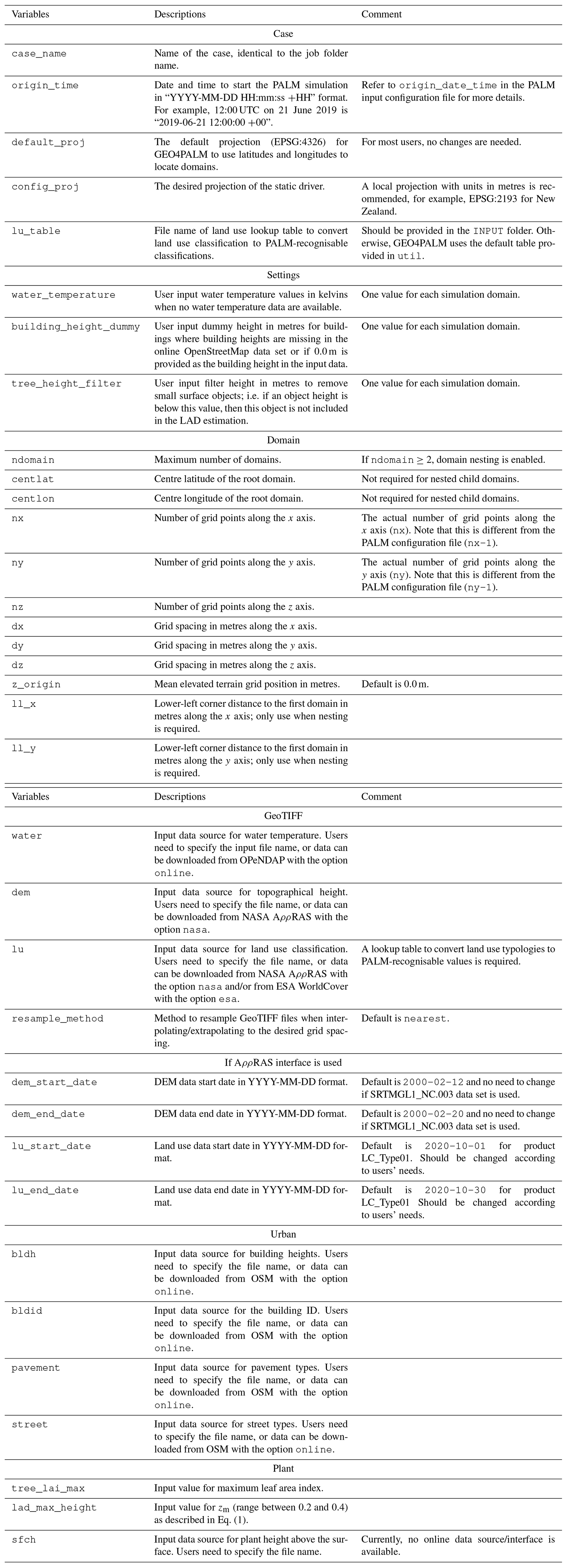
The hierarchy and data format of the variables in the static driver of PALM are described in PIDS (https://palm.muk.uni-hannover.de/trac/wiki/doc/app/iofiles/pids, last access: 20 June 2023) and by Heldens et al. (2020). Depending on the application, PALM simulations can include surface features such as buildings, pavements, and plants. In GEO4PALM, two settings are available for users to choose from. One is the default or the minimum setting, and the other allows users to add additional features for the urban surface and plant canopies. For the minimum setting, the static driver is incorporated with all the required variables to conduct a PALM simulation, while all the additional features are optional. Although GEO4PALM does not cover all the available features presented in PIDS, it includes most of the available features, including basic urban features such as buildings, pavements, and streets, which are sufficient to represent most urban and plant canopies. The variables covered by GEO4PALM are presented in Table 1.

Table 1 List of variables GEO4PALM can include in the PALM static driver. For more detailed descriptions of the variables, refer to Heldens et al. (2020) and PIDS (https://palm.muk.uni-hannover.de/trac/wiki/doc/app/iofiles/pids, last access: 20 June 2023).

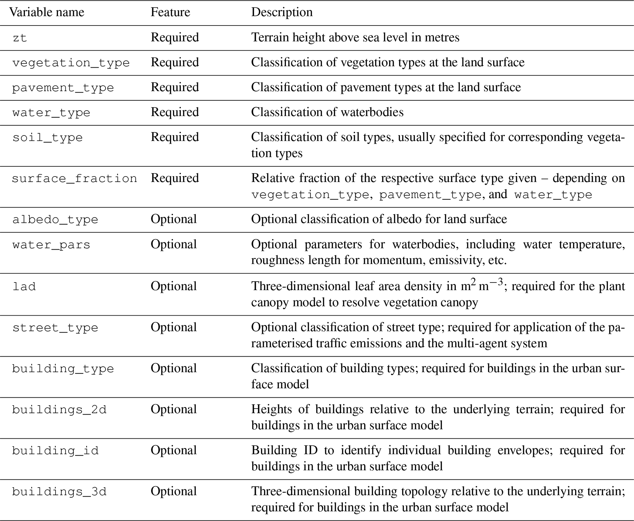
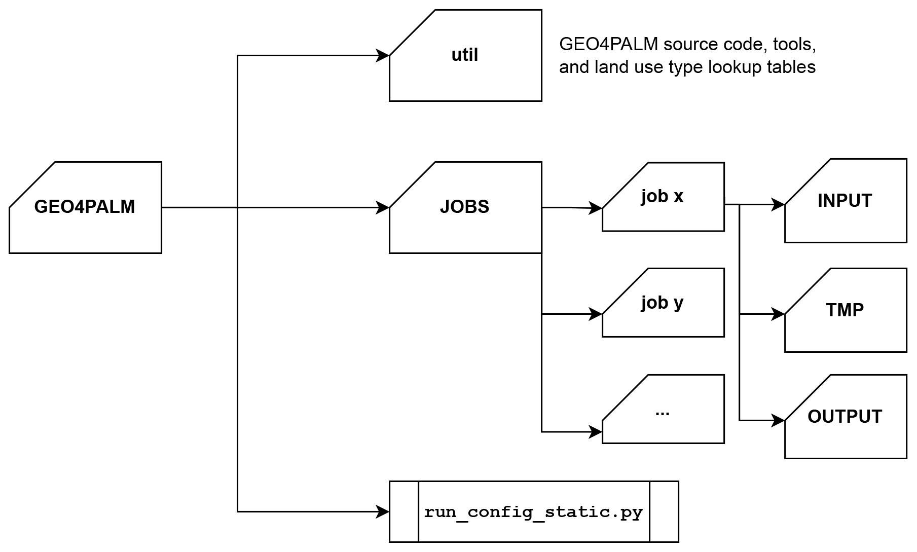
Figure 1 GEO4PALM file steering outline. The main executable script is run_config_static.py. The util folder contains all GEO4PALM utilities, including the source code, tools, and land use classification lookup table. Within the JOBS folder, each user-specified job is stored separately with input files in INPUT, temporary files in TMP, and output files in OUTPUT.

3 GEO4PALM framework

An early version of GEO4PALM was applied in simulations presented by Lin et al. (2021, 2023). However, this version (GEO4PALM v1.0) was only applicable for geospatial data for Ōtautahi / Christchurch, New Zealand. In this paper, several new features have been added to GEO4PALM v1.1. The new design of GEO4PALM v1.1 aims to (1) allow users to create static drivers for PALM simulations regardless of the geospatial data sources and (2) simplify the workflow of generating the static driver. The file steering structure of GEO4PALM is shown in Fig. 1. The main source code of GEO4PALM is stored in the util folder with the main executable Python script (run_config_static.py) located in the main directory. The JOBS folder allows users to create static driver files for multiple jobs (x, y, z, etc.). In each job directory, users must have an INPUT folder, which includes a configuration file, a land use type lookup table, and all input geospatial data files for the static driver. The TMP folder stores all temporary files, and all static driver files are created and stored in the OUTPUT folder.

Figure 2 Flowchart showing the code structure of GEO4PALM.

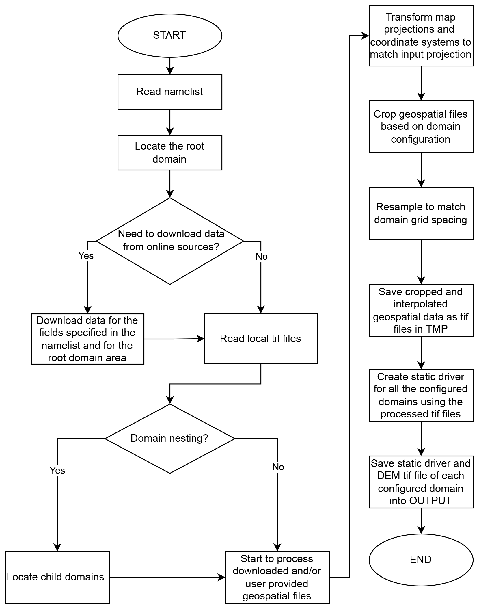
The framework of GEO4PALM is shown in Fig. 2. Users must at least provide a configuration file, which contains PALM domain configuration details and the data sources of static driver input. GEO4PALM uses Python packages including Xarray, Rasterio, rioxarray, GeoPandas, and geocube (Hoyer and Hamman, 2017; Gillies et al., 2019; Jordahl et al., 2020; Snow et al., 2022a, b) to process the geo-information data. When converting geospatial data into the static driver, GEO4PALM requires input files in GeoTIFF format, while no requirement is set regarding the spatial resolution and projection of the GeoTIFF files. The geospatial input data are resampled automatically based on the grid spacing values specified in the configuration file. Users have the freedom to choose the resampling method depending on their simulation needs. For details of the available options, users are referred to the Rasterio documentation (https://rasterio.readthedocs.io/en/stable/api/rasterio.enums.html#rasterio.enums.Resampling; last access: 23 June 2023). In addition to the GeoTIFF format, the shapefile format is one of the most common file types for geospatial data. Differently from the rasterised GeoTIFF files, the shapefiles are usually vectorised with multiple layers, and each layer has its own designated name, which varies with the data set. Due to the complexity of shapefiles, it is exhaustive to include shapefiles and all the embedded layers as a direct input in GEO4PALM. Therefore, a script shp2tif.py is provided as a GEO4PALM pre-processing tool for users to convert shapefiles to GeoTIFF format of the desired resolution (the finest in the input configuration file by default). This script converts one layer of the shapefile at a time, allowing users to choose the layer based on their applications. Table 2 explains all variables contained in the configuration file. A step-by-step guide for GEO4PALM and a sample configuration file are provided in Appendix A.

In the configuration file, users need to specify the desired geographic projection, domain configuration, and geospatial input data source for PALM simulations. If the desired projection of PALM simulations is not specified, GEO4PALM will use the nearest Universal Transverse Mercator (UTM) projection based on the latitude and longitude of the PALM domain centre given in the configuration file. To visualise PALM domain locations and to help users build the domain configuration easily, GEO4PALM is incorporated with a web-based interactive graphical user interface (GUI; Fig. 3). The GUI is generated by the palm_domain_utility.py script. This PALM domain utility allows users to render grid boxes of PALM domains over satellite and aerial imagery obtained from Environmental Systems Research Institute (Esri) World Imagery (https://geoviews.org/gallery/bokeh/tile_sources.html; last access: 19 June 2023) through open-source Python libraries including Panel and GeoViews (https://panel.holoviz.org/ and https://geoviews.org/; last access: 19 June 2023). The utility automatically checks and adjusts the domain configuration to avoid violations of rules for PALM domain nesting such as overlapping of domain boundaries and mismatching of the grid between parent and child domains. More details for using the PALM domain GUI are described in the GEO4PALM user manual (https://github.com/dongqi-DQ/GEO4PALM; last access: 7 November 2023).

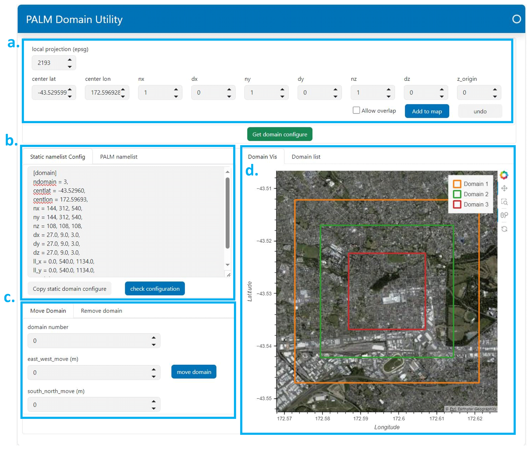
Figure 3 A screenshot of the web-based PALM domain utility GUI showing the domain configuration for the Ōtautahi / Christchurch case described in Sect. 4.3. Users can input domain configuration in the subtab (a). The GUI automatically generates configuration parameters for both GEO4PALM and PALM domain configuration in the subtab (b). Users can adjust the domain locations using the subtab (c). PALM domains are drawn over the interactive satellite imagery in the subtab (d).

Users are not required to have a full set of input data. For each geospatial input field, users can provide their own data in GeoTIFF or shapefile format and download data from online sources when some of the data sets are not locally available. For geospatial files provided by users, one needs to specify the file name in the configuration file. If one desires to use online data, the data source should be specified. For the time being, we provide several interfaces to download data sets with global coverage. Water temperature, the digital elevation model (DEM), and land use are the three mandatory elements to create a static driver. Water temperature is an important factor which can have an impact on boundary layer structure (e.g. Mahrt and Hristov, 2017), while by default PALM prescribes a water temperature of 283.0 K for all waterbodies. Therefore, water temperature is required in GEO4PALM. Users can provide their own water temperature map in a GeoTIFF file or a prescribed water temperature in the configuration file for all waterbodies in the simulation domains. Alternatively, users can use the online sea surface temperature (SST) data set downloaded by GEO4PALM. As SST is widely available across various global data sets, we provide an interface to download SST data to represent water temperature for waterbodies in the GEO4PALM static driver. The SST data (resolution of 0.01^∘) are obtained using the Earthdata Common Metadata Repository (CMR) API operated by the National Aeronautics and Space Administration (NASA), which is linked to the OPeNDAP interface (Open-source Project for a Network Data Access Protocol; https://lpdaac.usgs.gov/tools/opendap/; last access: 20 May 2023). The NASA data sets are available globally, and users are required to register an account to use the data freely. By default, GEO4PALM downloads version 4.1 of the Multi-scale Ultra-high Resolution (MUR) of the Group for High Resolution Sea Surface Temperature (GHRSST) Level-4 analysis provided by NASA's Jet Propulsion Laboratory (NASA/JPL, 2015; Chin et al., 2017). The water temperature is obtained from the grid point of the SST data set nearest to the PALM simulation domains. To download and use this data set, users must specify online in the configuration file for the variable water. The date and time of the SST data should be specified using the parameter origin_time in the [case] section. If users have spatial water temperature data available for waterbodies in GeoTIFF format, they can specify the data file name in the configuration file for the variable water. Users are also allowed to prescribe a fixed water temperature for each simulation domain using the water_temperature parameter in the [settings] section.

The DEM (spatial resolution of 30 m) and land use classification are available to download from the Application for Extracting and Exploring Analysis Ready Samples (AρρEEARS; https://appeears.earthdatacloud.nasa.gov/; last access: 7 November 2023) operated by NASA. The DEM is the product of NASA Shuttle Radar Topography Mission 1 arcsec NetCDF V003 (SRTMGL1_NC.003) acquired by spaceborne radar (Rabus et al., 2003). For the NASA data, users may provide the start and end date for the data acquisition such that the land use is representative of the simulation period. GEO4PALM source code provides a lookup table (Table B1) for the MODIS Land Cover Type product (AρρEEARS product code: LC_type1), which converts the land use classification to PALM-recognisable values. The MODIS Land Cover Type product supplies global land cover maps at 500 m spatial resolution dated from 2001 (Friedl and Sulla-Menashe, 2019). More options for land use classification data sources provided by NASA refer to AρρEEARS online documentation (https://appeears.earthdatacloud.nasa.gov/; last access: 7 November 2023). If users desire to download and use AρρEEARS data sets, they must specify nasa in the configuration file for the variables dem and/or lu.

In addition to the AρρEEARS interface, GEO4PALM incorporates the application programming interface that connects to the worldwide land cover mapping data products (WorldCover; https://esa-worldcover.org/en; last access 7 November 2023) operated by the European Space Agency (ESA). The ESA WorldCover data have a spatial resolution of 10 m (Zanaga et al., 2021, 2022). Users must register a free account to obtain data from ESA. A lookup table (Table B2) for PALM-readable conversion is provided in the GEO4PALM source code. For the usage of ESA data, users are required to specify esa in the configuration file for the variable lu. In addition to the lookup tables for NASA and ESA data, the GEO4PALM source code provides a lookup table (Table B3) for the New Zealand Land Cover Database (LCDB) V5.0 (Landcare Research, 2020). All the lookup tables are presented in Appendix B.

All urban and plant fields can be left blank (“”) in cases where users do not require such features in the static driver. If users desire to have other land surface features, GEO4PALM can process data for the urban surface model and plant canopy model. In PALM, urban surfaces include pavements, buildings, and streets. Although according to PIDS v1.12, the typology of streets is represented by the variable pavement_type and the variable street_type is only used for the chemistry model in PALM, GEO4PALM still includes the variable street_type such that the static driver can be used for simulations that require the chemistry model and/or the multi-agent system. Like the DEM and land use data, users can either provide their own GeoTIFF data or choose to download data online. If users wish to provide their own data, they must provide GeoTIFF files with building height at the building location, building ID for each building, PALM-recognisable pavement types for each pavement, and/or PALM-recognisable street types for each street, separately. Otherwise, users can specify osm for the urban variables in the configuration file to download data from OpenStreetMap (OSM; https://www.openstreetmap.org/; last access: 7 November 2023). GEO4PALM uses the OSMnx package (Boeing, 2017) to obtain data from OSM. Downloaded OSM data sets are converted to PALM-recognisable data by GEO4PALM using the conversion described by Heldens et al. (2020). Note that OSM also provides land use classification but does not have a good spatial coverage for many regions in the world. Therefore, GEO4PALM currently does not support OSM land cover data. Users are encouraged to use the OSM land cover data set with a modified land use type conversion table like those shown in Appendix B if their PALM simulations are conducted for regions with good spatial coverage of OSM land cover data. GEO4PALM is adaptable to any land use data provided in shapefile or GeoTIFF format.

For plant canopy, GEO4PALM currently only supports leaf area density (LAD; Lalic and Mihailovic, 2004) calculations based on vegetation height provided in the GeoTIFF files. To avoid noise from other surface geometry, GEO4PALM applies an automatic process in which surface objects with heights less than the filter (tree_height_filter in Table 2) are removed. With this filter, objects like cars or fences are not included as vegetation. The default value of the filter is 1.5 m, and users can adjust the value in the configuration file. With high-quality data, this noise filter can be set to a desired low value (≥0.0 m) such that low objects, like grass, long grass, and bushes, can be included and represented in PALM simulations. The LAD calculation is adopted from PALM CSD (Heldens et al., 2020) and is based on the equation proposed by Lalic and Mihailovic (2004) as follows:

$$\begin{array}{}\text{(1)}& \begin{array}{rl}\mathrm{LAD}\left(z\right)& ={\mathrm{LAD}}_{\mathrm{m}}{\left({\displaystyle \frac{h-z_{\mathrm{m}}}{h-z}}\right)}^n\exp \left[\left(\mathrm{1}-{\displaystyle \frac{h-z_{\mathrm{m}}}{h-z}}\right)n\right]\\ & \left[{\mathrm{m}}^{\mathrm{2}}{\mathrm{m}}^{-\mathrm{3}}\right],\end{array}\end{array}$$

where LAD_m is the maximum LAD, h is the tree height, z_m is the height where LAD reaches LAD_m, and n=6 when z<z_m and n=0.5 when z≥z_m. According to Kolic (1978) and Lalic and Mihailovic (2004), the normalised value of z_m ranges from 0.2 to 0.4 depending on the tree type. Currently, GEO4PALM only allows users to provide a fixed value of leaf area index (LAI; tree_lai_max in Table 2) and z_m (lad_max_height in Table 2) values as input. LAI is recognised as the integration of LAD over the tree height (h). To derive LAD at each vertical level, GEO4PALM uses the given LAI and z_m with the integral form of Eq. (1) (refer to Lalic and Mihailovic, 2004, for more details). GEO4PALM automatically scales LAD based on the height of the vegetation canopy at individual grid points. This approach does not take account of spatial variation in LAD for different tree species, while it is still useful in cases where no LAD or LAI data are available. For cases in which LAD or LAI information is available, users are advised to adjust the code to directly read the spatial LAD/LAI information. However, to the best of our knowledge, no globally available vegetation height data, along with plant canopy data, are currently free to obtain from any online sources. Therefore, GEO4PALM does not provide any online interface for this purpose. One possible solution to obtaining vegetation height is to calculate surface objects' height using the digital surface model (DSM) and DEM. In addition to the information on ground surface altitude contained in the DEM, the DSM supplies the heights of all surface objects, such as buildings and trees.

Once users have provided all required information in the configuration file along with their own geospatial data where applicable, GEO4PALM downloads and/or processes the input data to create the static driver. GEO4PALM allows users to configure nested domains and use different input data for each domain. To reduce the learning curve, the domain nesting configuration is similar to PALM's nesting module, in which the nested domain location is determined by the distance of the lower-left corners between the root domain and child domains. PALM's own input and output files can contain geospatial information, while the geospatial projection references sometimes may not be included accurately in a NetCDF file. Geospatial coordinates with correct geospatial projection could be important in real-world applications, especially when comparing PALM results to observations. To overcome this potential issue, instead of providing geospatial information in the NetCDF files, a GeoTIFF file with coordinate information is created by GEO4PALM along with each static driver. We recommend that GEO4PALM users use the GeoTIFF file to better reference the geospatial coordinate. For more details and examples, users are referred to the Supplement, which contains the input files for the case studies presented in Sect. 4.

Table 2 Variables descriptions of the GEO4PALM input configuration file.

4 Examples of real-world applications

4.1 Model and simulation configuration

As mentioned in Sect. 3, the aim of GEO4PALM is to allow users to use geospatial data for their PALM simulations seamlessly. Users may have data ready locally in GeoTIFF or shapefile format, or they can download all geospatial data freely for any location. Several other studies have used the input data described in this article and the earlier versions of GEO4PALM. For example, the static input generated by GEO4PALM was used for Christchurch Airport to demonstrate applications of the WRF4PALM offline nesting tool (Lin et al., 2021). Lin et al. (2023) have used GEO4PALM-generated static input for fog research over the city of Ōtautahi / Christchurch.

In this section, we present two examples, both using GEO4PALM and PALM CSD, to demonstrate the performance and compatibility of GEO4PALM. One example is Berlin, Germany (52.516615^∘ N, 13.402782^∘ E), and the other is Ōtautahi / Christchurch, New Zealand (43.529599^∘ S, 172.596928^∘ E). We have used the online API for both cases to obtain geospatial input. For Berlin, we have geospatial data sets prepared and stored locally containing topography, streets, buildings, waterbodies, vegetation, etc., at 2 m resolution. These data have been processed by the German Space Agency (DLR) similarly to those described by Khan et al. (2021) and Heldens et al. (2020). Hereafter, we refer to the local data sets for Berlin as the DLR data sets. We have used the same DLR data sets to run both PALM CSD described by Heldens et al. (2020) and GEO4PALM with a map projection of EPSG:25833 (ETRS89/UTM zone 33N) to match the projection coded in PALM CSD. At present, PALM CSD only supports 10 UTM projections between zone 28N and zone 37N or a pre-processed rectangle map projection. Therefore, for Ōtautahi / Christchurch, we pre-processed all the local data to the map projection of EPSG:2193 (New Zealand Transverse Mercator) using geographic information system (GIS) software and the tools in GEO4PALM. Then, the corresponding GeoTIFF files were processed into PALM-CSD-compatible NetCDF files. Since PALM CSD does not provide land use classification conversion from other data sources, we first used GEO4PALM to convert our land use input data set to PALM-recognisable land use types. Then, we used GIS software with additional Python scripts to make our land use data sets compatible with PALM CSD.

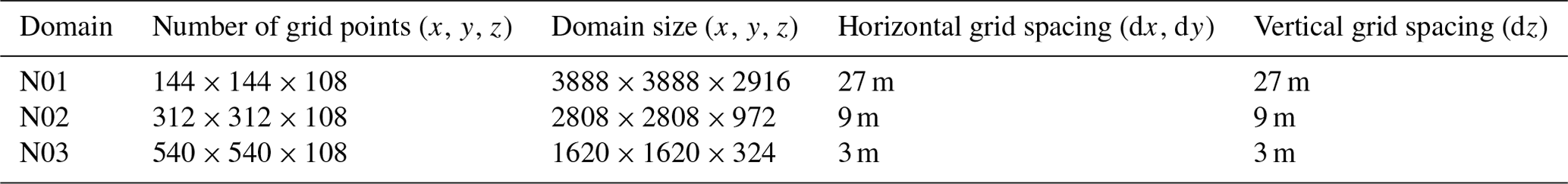
Table 3 gives an overview of the simulations conducted for Berlin and Ōtautahi / Christchurch. Overall, we conducted six simulations, comprising three simulations for each of the two cities. The three simulations for Berlin are denoted Berlin_CSD, Berlin_GEO, and Berlin_OL, which used static drivers generated by PALM CSD, GEO4PALM with the DLR data sets, and GEO4PALM with online data sets, respectively. The three simulations for Ōtautahi / Christchurch are denoted Chch_CSD, Chch_GEO, and Chch_OL, which used static drivers generated by PALM CSD with local data sets, GEO4PALM with local data sets, and GEO4PALM with online data sets, respectively. For demonstration purposes, both examples have identical domain dimensions and grid spacing (shown in Table 4). All geospatial input data were resampled to match the grid spacing of the simulations. To demonstrate the LAD calculation in GEO4PALM, we used tree_lai_max =5.0 and lad_max_height =0.4, corresponding to pine trees, for both Berlin_GEO and Chch_GEO. The initialisation time was set to 00:00 UTC on 1 January 2021 for Ōtautahi / Christchurch and 12:00 UTC on 1 January for Berlin, which is midday summertime for Ōtautahi / Christchurch and around midday wintertime for Berlin. The simulation time is 6 h for both simulations. Due to the high computation cost with fine grid spacings, here we only performed simulations using domain nesting with the finest grid spacing at 3 m, while GEO4PALM can generate a static driver with grid spacings finer than 1 m, depending on the data source.

We used the PALM model system 22.10 to conduct the simulations. For demonstration purposes, all simulations were initialised with idealised forcing. A northerly was prescribed with a wind speed of 4 m s⁻¹. At the initialisation, the surface potential temperature is 295.65 K with no vertical gradient in the first 2000 m from the surface and a vertical gradient of 0.3 K per 100 m for the levels above 2000 m up to the top boundary. The prognostic equation for the water vapour mixing ratio is switched off. Periodic lateral boundary conditions are used with the clear-sky radiation scheme. The radiative transfer model (RTM; Krč et al., 2021) and land surface model (LSM; Gehrke et al., 2021) were switched on for all domains. The urban surface model (USM; Resler et al., 2017) and plant canopy model (PCM; Maronga et al., 2020) are only switched on for the child domains (N02 and N03).

Table 3 Overview of simulations for Berlin and Ōtautahi / Christchurch.

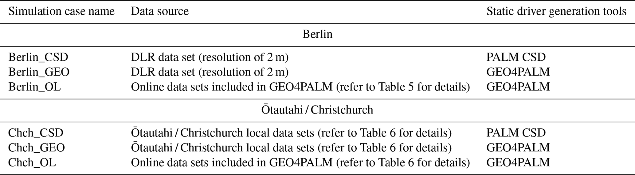
Table 4 Nested domain dimension summary. Here, x refers to the west–east coordinate, y refers to the south–north coordinate, and z refers to the vertical coordinate.

4.2 Case study for Berlin

This section demonstrates a case study to compare the static drivers created by PALM CSD, GEO4PALM with local data, and GEO4PALM with online data. The input data sources used in GEO4PALM are listed in Table 5. For Berlin_CSD and Berlin_GEO, the data were processed by DLR. For details of the DLR data sets and PALM CSD, refer to Khan et al. (2021) and Heldens et al. (2020). As water temperature was not included in the DLR data set, we used GEO4PALM to obtain water temperature via the Earthdata API for Berlin_GEO. Regarding Berlin_OL, the only user input is the configuration file. GEO4PALM handled all data downloading from online sources, including the global GHRSST data, NASA 30 m DEM data (SRTMGL1_NC.003), ESA WorldCover land use classification data, and OSM urban data sets.

Khan et al. (2021)Heldens et al. (2020)Khan et al. (2021)Heldens et al. (2020)Khan et al. (2021)Heldens et al. (2020)Khan et al. (2021)Heldens et al. (2020)Khan et al. (2021)Heldens et al. (2020)Khan et al. (2021)Heldens et al. (2020)Khan et al. (2021)Heldens et al. (2020)(Boeing, 2017)(Boeing, 2017)(Boeing, 2017)(Boeing, 2017)

Table 5 Geospatial input data for GEO4PALM used in the Berlin case study. Refer to Khan et al. (2021) and Heldens et al. (2020) for details of data sources for Berlin_CSD.

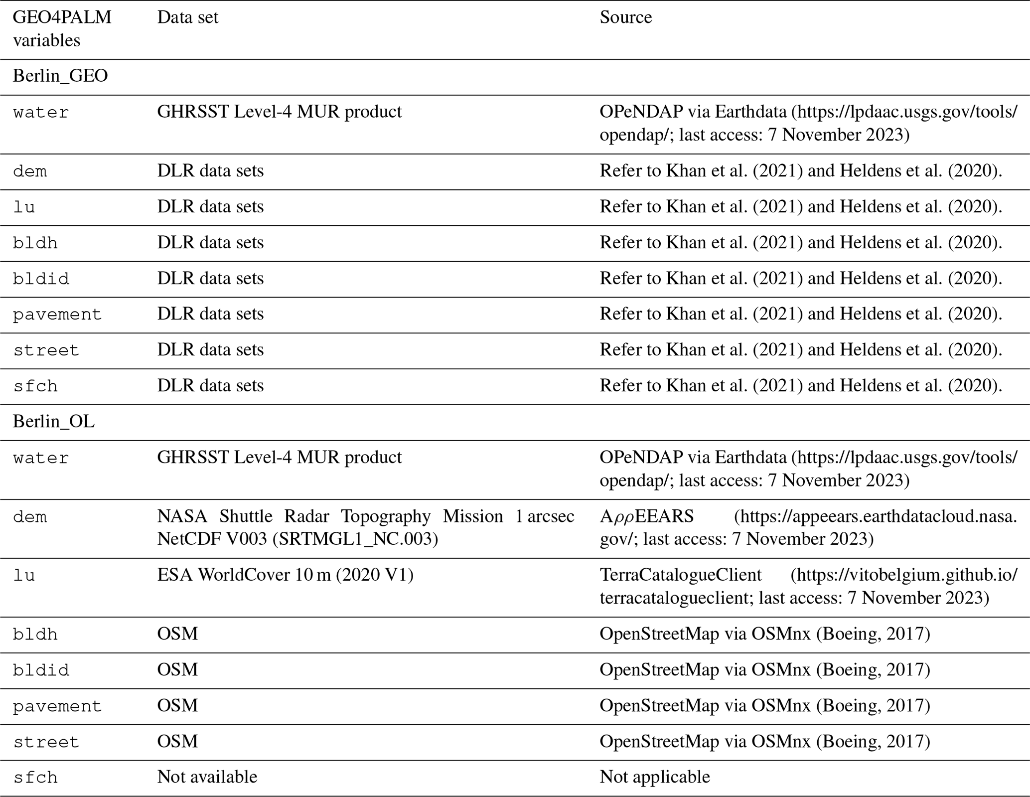
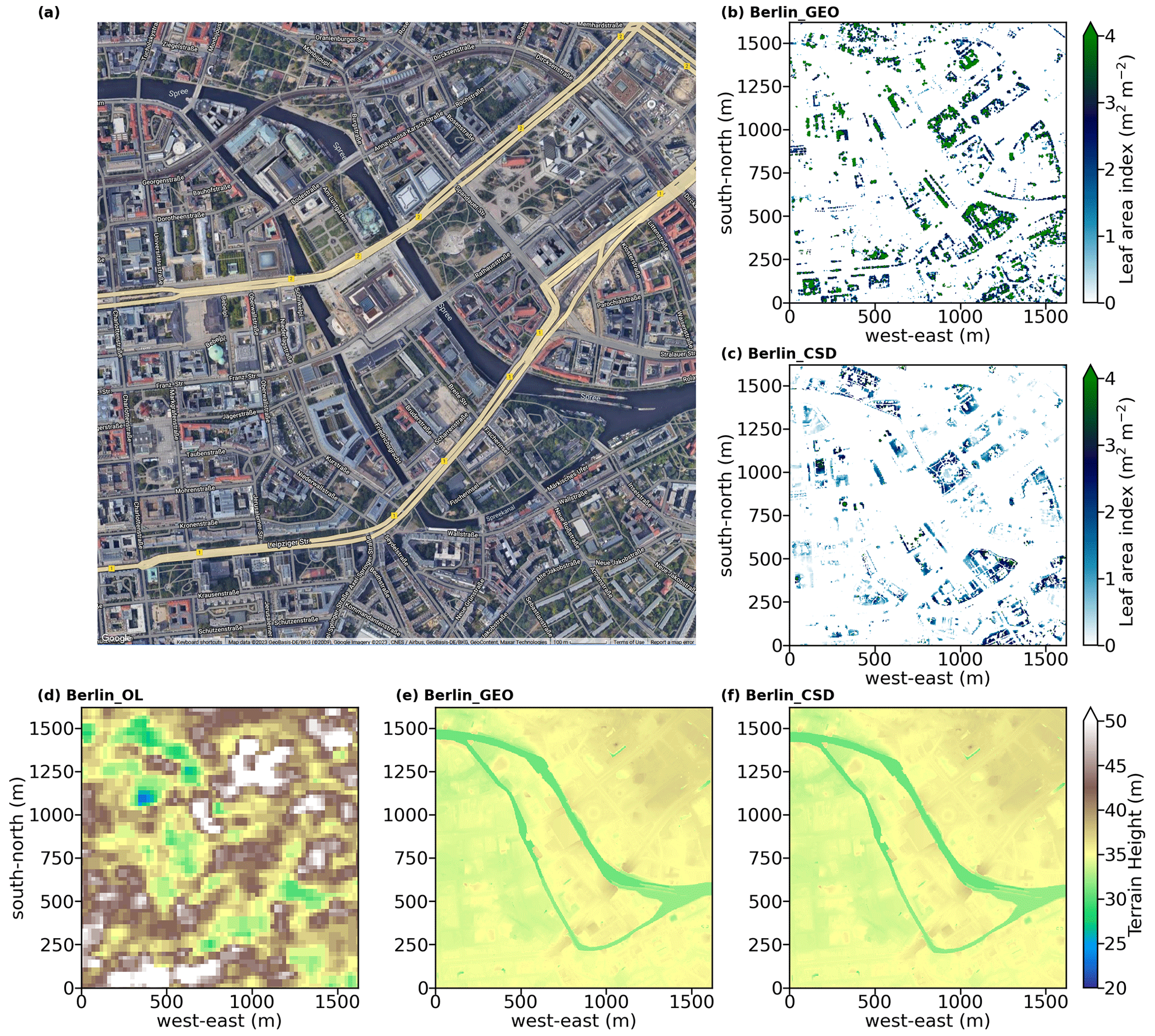
Figure 4 (a) Satellite images showing domain location of the nested domain N03 for the Berlin case (© Google Earth). Domain centre is located near the Humboldt Forum in central Berlin, Germany. The horizontal cross-sections of static input data: (b–c) LAI (vertically integrated LAD) and (d–f) terrain height. For data sources refer to Table 4. No LAI data are displayed for Berlin_OL, as no online data source is available for the estimation of LAD.

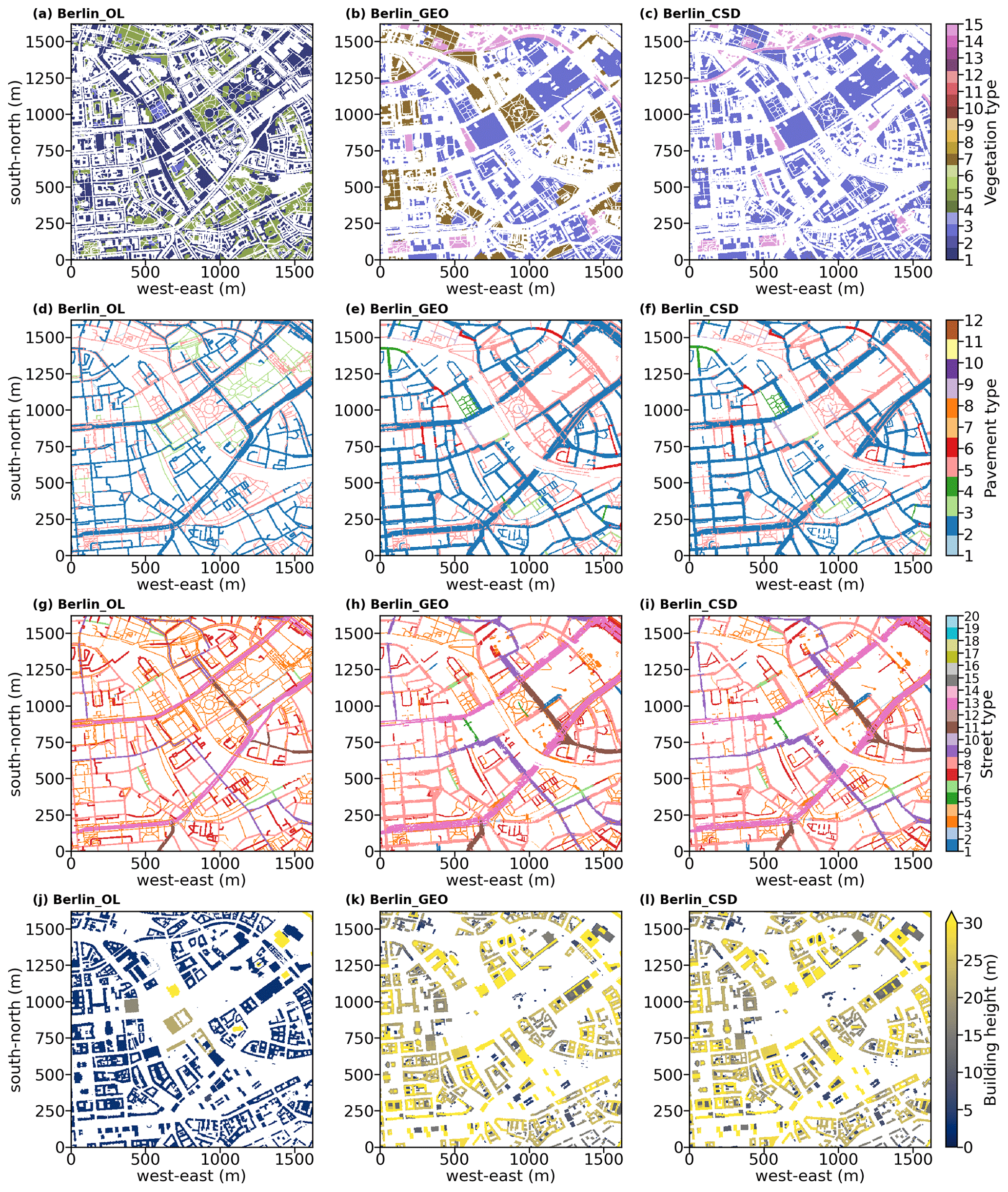
Figure 5 Static input data of the nested domain N03 for the Berlin case: (a–c) vegetation type, (d–f) pavement type, (g–i) street type, and (j–l) building height. Refer to the panel label for the corresponding simulation. For data sources refer to Table 5.

The domain location and static driver data for Berlin_CSD, Berlin_GEO, and Berlin_OL are shown in Figs. 4 and 5. In Berlin_OL, several buildings are included in the simulation domain. However, the OSM data (used in the Berlin_OL simulation) do not contain building height for most buildings. Therefore, buildings with no height data available were assigned a height of 3.0 m for demonstration purposes. LAI, the vertically integrated LAD, shows areas with plant canopy in Fig. 4b and c. For the Berlin_OL case, LAD was not included in the static driver input, since we do not have any DEM or DSM with spatial resolution finer than 30 m. The LAI calculated by GEO4PALM (Fig. 4b) is higher than the one calculated by PALM CSD (Fig. 4c). In Berlin_GEO, the vegetation patch height data were directly used by GEO4PALM to estimate LAD, without considering vegetation type. In Berlin_CSD, however, vegetation type and the simulation season were considered. A lot of data processing is required to pre-process vegetation data for PALM CSD. For the estimation of LAD, at least the vegetation height, vegetation type, and LAI data are required. Considering the inconsistency in data sources and quality worldwide, GEO4PALM adopts the simplified method to calculate LAD. Both GEO4PALM and PALM CSD can be modified further by users depending on their modelling needs.

Berlin_GEO and Berlin_CSD present similar features in terrain heights (Fig. 4e and f) in which the shapes of rivers are distinguishable. However, the terrain heights in Berlin_OL (Fig. 4d) do not contain many details due to the coarse resolution of its data source. The online DEM data only have a spatial resolution of 30 m. Berlin_GEO and Berlin_CSD used the same geospatial input, and hence, the topography data for the two cases are identical. It should be noted that PALM CSD offers an option to modify the terrain height of the child domains to follow the average values of their corresponding parent domain, allowing for a smoother transition of the flow at the nested child domains' lateral boundaries. After this modification, PALM CSD can be configured to adjust the topography height onto the simulation domain's vertical levels. Currently, such adjustments are not included in GEO4PALM. GEO4PALM adopts the DEM directly and lets PALM itself process and convert topography into the simulation grid. These topography adjustment features are switched off for the comparison between PALM CSD and GEO4PALM presented here.

The vegetation type in Berlin_OL (Fig. 5a) also has a coarser resolution compared to Berlin_GEO (Fig. 5b) and Berlin_CSD (Fig. 5c) because the spatial resolution for the ESA land use data is 10 m. The difference in the vegetation-type classification between Berlin_OL and the other two simulations could be due to the conversion between the ESA WorldCover data set and PALM. Users are referred to Table B2 for the conversion, which can be edited depending on users' needs. Comparing Berlin_GEO (Fig. 5b) to Berlin_CSD (Fig. 5c), one can notice that vegetation patches classified as type 7 (deciduous broadleaf trees; brown patches in Fig. 5b) in Berlin_GEO are classified as type 3 (short grass; light purple in Fig. 5c) in Berlin CSD. This is caused by the adjustments applied in PALM CSD. It corrects vegetation type when a vegetation height is available and is indicative of low-lying plant cover. PALM CSD also alters the vegetation type for grid points where LAD data are available, i.e. where the plant canopies are resolved. This is to avoid numerical issues when using a high roughness length with small vertical grid spacing. In addition, a tall vegetation type with high roughness length plus the resolved plant canopies could over-represent the drag of the vegetation. Subsequently, the flow reduction may be overestimated. This feature is currently not available in GEO4PALM.

The pavement type and street type presented in Berlin_OL are generally similar to in Berlin_GEO and Berlin_CSD. As the widths of pavements and streets were generated automatically in Berlin_OL by GEO4PALM, some of the details, such as the width and type of each pavement and street, are of lower fidelity in Berlin_OL compared to those in Berlin_GEO and Berlin_CSD. This is similar regarding buildings. The structures and locations of buildings in Berlin_OL align with those in Berlin_GEO and Berlin_CSD. However, the DLR geospatial data do not include the Berlin Palace (as shown in the centre of Figs. 4a and 5j–l), while this building is present in Berlin_OL (Fig. 5j). This building was recently reconstructed and hence is not included in the DLR data set and subsequently not included in Berlin_GEO and Berlin_CSD.

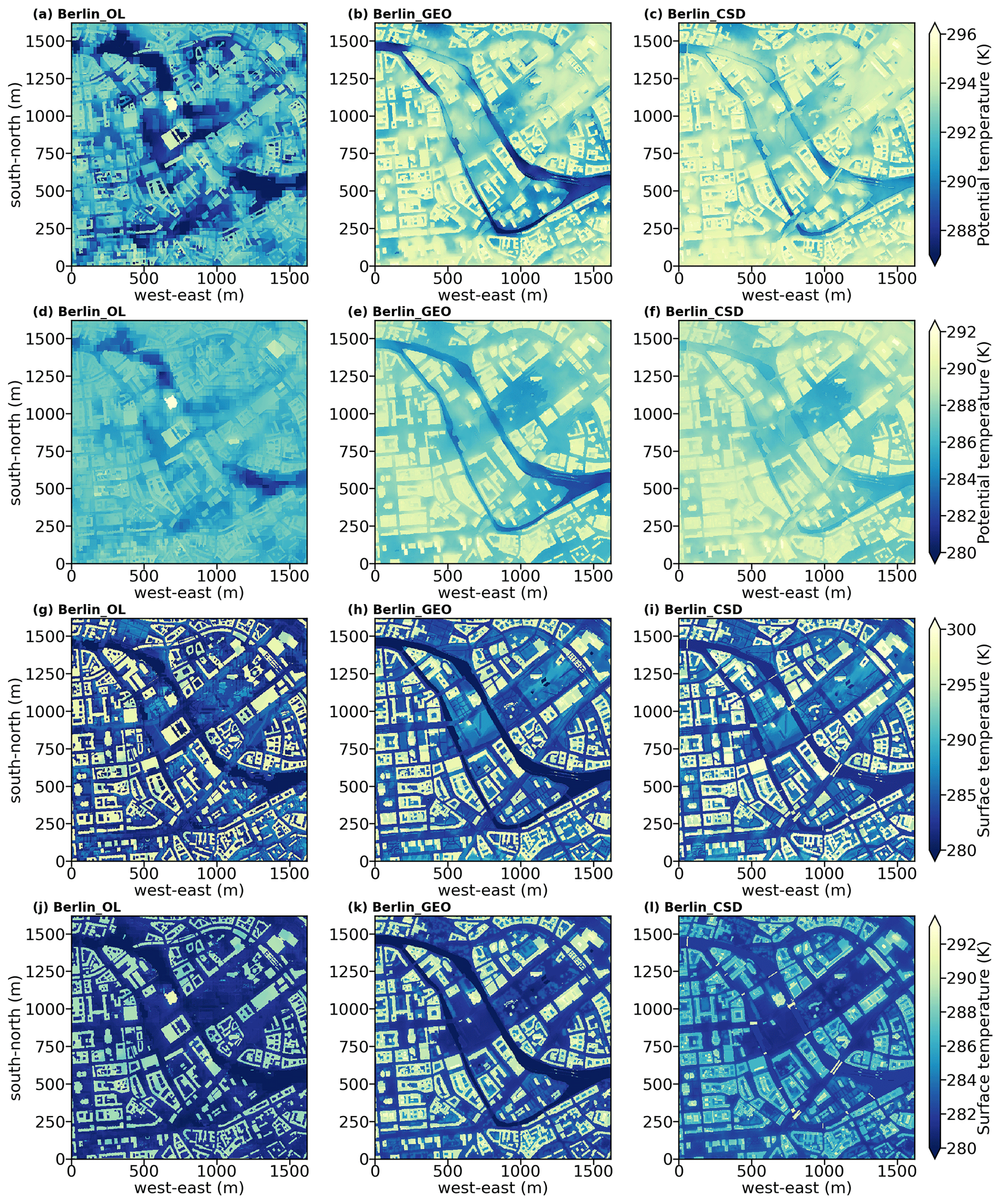
Figure 6 Horizontal cross-sections of simulation results for the Berlin case: (a–f) potential temperature at 2 m (θ_2m) and (g–l) surface temperature (T_sfc). Panels (a)–(c) and panels (g)–(j) are averages of the second hour of the simulation. Panels (d)–(f) and panels (j)–(l) are averages of the last hour of the simulations. Refer to the panel labels for the corresponding simulation.

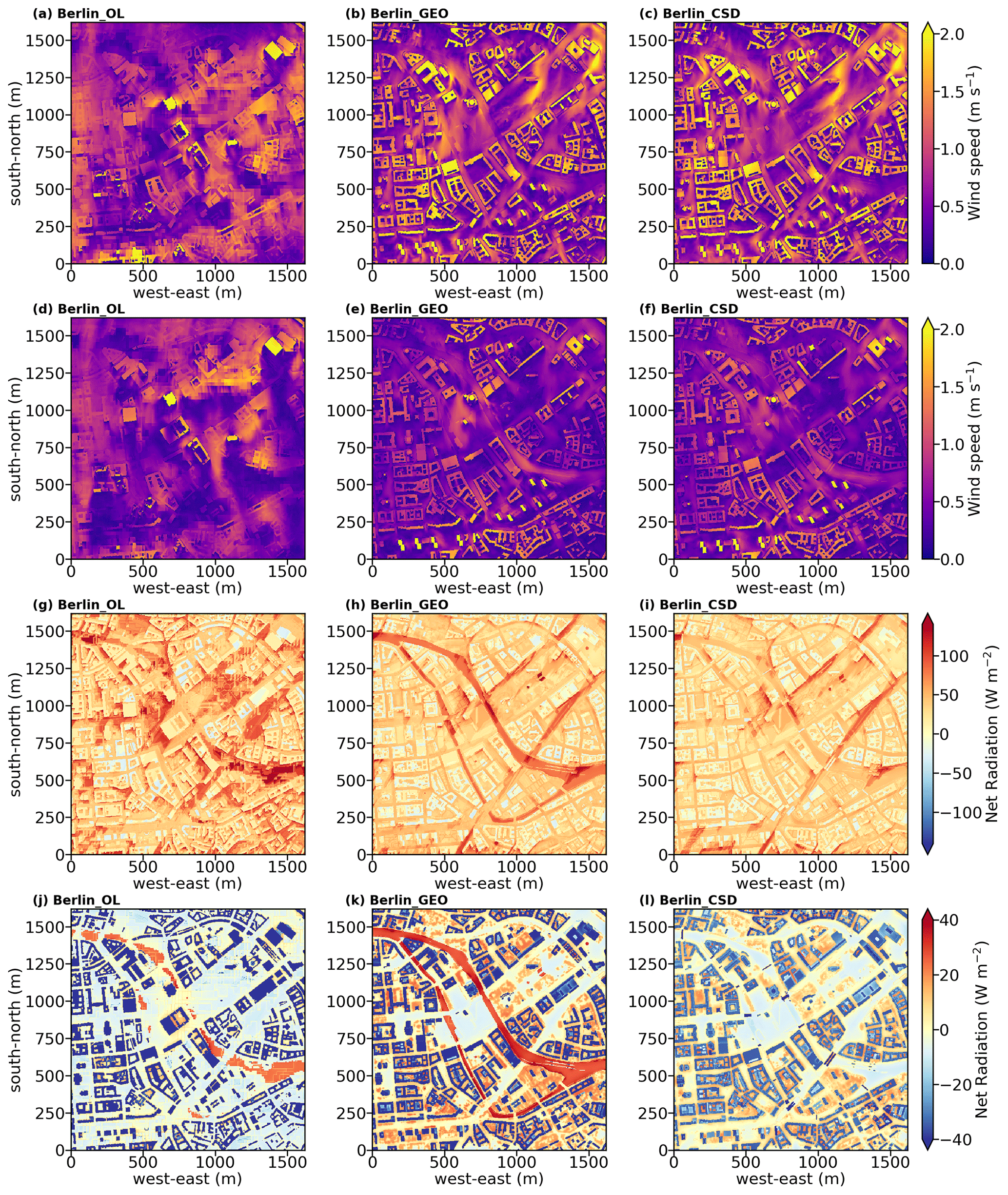
Figure 7 Similar to Fig. 6 but for wind speed at 10 m (WS_10 m) (a–f), and surface net radiation (R_net) (g–l). Refer to the panel labels for the corresponding simulation.

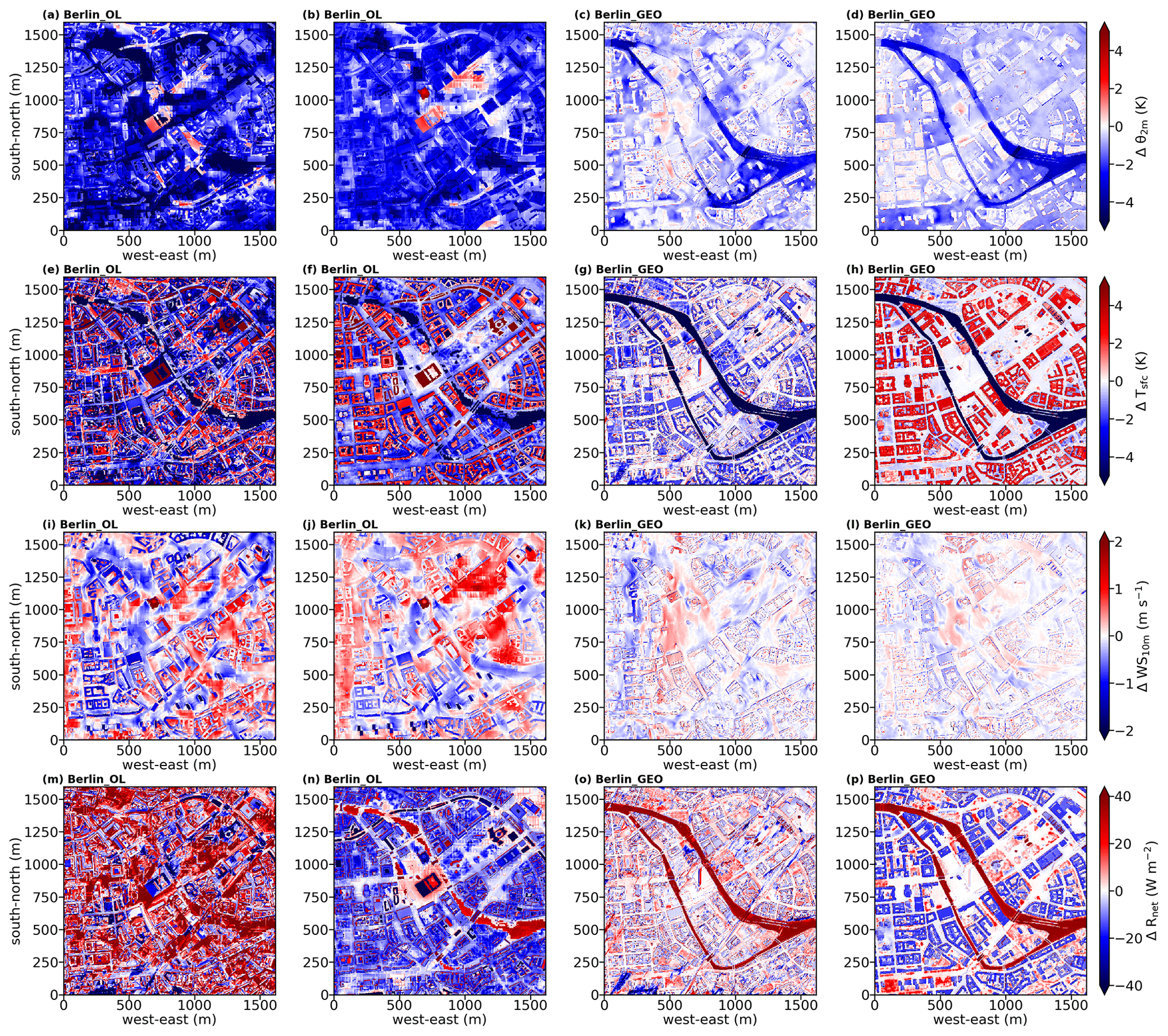
Figure 8 Differences in simulation results (shown in Figs. 6 and 7) between GEO4PALM simulations and PALM CSD simulation. The differences are results of GEO4PALM simulations subtracted from the PALM CSD simulation: (a–d) differences in θ_2m, (e–h) differences in T_sfc, (i–l) differences in WS_10 m, and (m–p) differences in R_net. From left to right, the first and the second columns show the differences between Berlin_OL and Berlin_CSD for the second and sixth hour of the simulations, respectively. The third and fourth columns show the differences between Berlin_GEO and Berlin_CSD for the second and sixth hour of the simulations, respectively. Refer to the panel labels for the corresponding simulation.

Figures 6 and 7 illustrate the horizontal cross-sections of the simulation results. These results are hourly averages for the second and sixth (i.e last) hour of the simulations. The variables displayed include 2 m potential temperature (θ_2m), surface temperature (T_sfc), surface net radiation (R_net), and 10 m wind speed (WS_10 m) and direction. To compare the simulation results between GEO4PALM and PALM CSD, the differences between Berlin_OL and Berlin_CSD and between Berlin_GEO and Berlin_CSD are shown in Fig. 8. In all simulations, R_net and T_sfc are strongly dependent on the land surface type and surface canopy. Comparing Berlin_OL to Berlin_GEO, the differences show the impact of the geospatial data input. The topography input data for Berlin_OL have a resolution of 30 m. The coarse topography in Berlin_OL creates box-like features, especially for θ_2m (see Figs. 6a and 8a) and R_net (Fig. 7g) at the beginning of the simulation. Although Berlin_OL captures the building outlines in the simulation domain, the lack of accurate building height data leads to an underestimation of θ_2m (Fig. 8b) and an overestimation of WS_10 m (Fig. 8j) compared to Berlin_CSD. In GEO4PALM, all buildings are configured as type 3 (residential buildings built after 2000) by default because we currently do not have a good local building-type data set to use as a reference. As a result of different building-type data sets, Berlin_OL shows an overestimation of T_sfc compared to Berlin_CSD (Fig. 8f). In addition, as the land use input data have a grid spacing of 10 m for Berlin_OL, the waterbodies were not presented with good fidelity in Berlin_OL, compared to Berlin_GEO and Berlin_CSD. This is reflected in the simulated R_net in Fig. 6j. As Berlin_OL uses a completely different geospatial data set compared to Berlin_CSD, the values of R_net in Berlin_OL for non-building areas are significantly higher than those in Berlin_CSD (Fig. 8m) in the second simulation hour. The differences are still considerable in the last simulation hour (Fig. 8n), suggesting the importance of the input data. The presence of the Berlin Palace in Berlin_OL shows a strong impact on the simulated temperature, wind, and net radiation. In more realistic applications, users should be careful about the geospatial data acquisition dates, especially in urban environments where building reconstructions frequently occur.

For a more direct comparison between GEO4PALM and PALM CSD, the results of Berlin_GEO and Berlin_CSD are presented. For the comparison in the second simulation hour, Berlin_GEO coincides with more variations in T_sfc and R_net than in θ_2m and WS_10 m (Fig. 8). This is because T_sfc and R_net are more sensitive to the differences in the input water temperature, the input building types, adjustments applied in vegetation types, and LAD estimation methods. PALM CSD allows users to input the spatial distribution of water type and water temperature. Otherwise, it uses the default water temperature of 283.0 K embedded in the code. Similarly to PALM CSD, GEO4PALM allows a spatial input of water temperature. However, we do not have water temperature data available. For the Berlin case study, GEO4PALM obtained water temperature from the GHRSST data, which is 275.0 K. For comparison and demonstration purposes, we did not modify the default water temperature in PALM CSD, while users can modify the source code for their simulations. Such a difference in water temperature leads to significant contrasts in T_sfc (Fig. 8g–h) and R_net (Fig. 8o–p) between Berlin_GEO and Berlin_CSD. Over the river, θ_2m is also lower in Berlin_GEO. The same as Berlin_OL, only one building type is used in Berlin_GEO. This leads to higher T_sfc in Berlin_GEO later in the simulation (Fig. 8h). The differences in the building type also lead to a negative bias in the R_net differences for building areas in Berlin_GEO.

Adjustments in the vegetation type are evident in the surface variables (T_sfc and R_net; Fig. 8g–h and o–p), especially at the beginning of the simulations (Fig. 8g and o). Excluding the waterbodies and buildings, the blue patches in Fig. 8g coincide with the brown patches in the vegetation types of Berlin_GEO shown in Fig. 5b. Without the adjustments in the vegetation type, these vegetation patches in Berlin_GEO lead to a positive bias in R_net compared to Berlin_CSD (Fig. 8o). In the last simulation hour, the cold biases in T_sfc in Berlin_GEO over the vegetation patches are less significant (Fig. 8h). Regarding R_net, the positive biases resemble the LAI patterns of Berlin_GEO shown in Fig. 4b, showing the potential impact of inaccurate LAD input. The signal of the adjusted vegetation type, however, is not clear in WS_10 m, as shown in Fig. 8k–l. Without the vegetation-type adjustment, the wind speed is expected to be lower in Berlin_OL, while we cannot identify such an impact from Fig. 8k–l. More investigation is required to determine the appropriate adjustment in vegetation types.

Overall, the static driver generated by GEO4PALM and, subsequently, the simulation fidelity of PALM are highly dependent on the input geospatial data quality. With high-quality data, GEO4PALM can create static drivers (Berlin_GEO) that are comparable to PALM CSD (Berlin_CSD). Without local data, GEO4PALM can only represent the simulated environment with limited details, as presented in Berlin_OL. The lack of building height information and the coarse resolution of the online data sets may not be suitable for a realistic simulation in the urban environment. These data sets, however, could be useful for coarse simulations, for example, the parent domains of the focused simulation area.

4.3 Case study for Ōtautahi / Christchurch

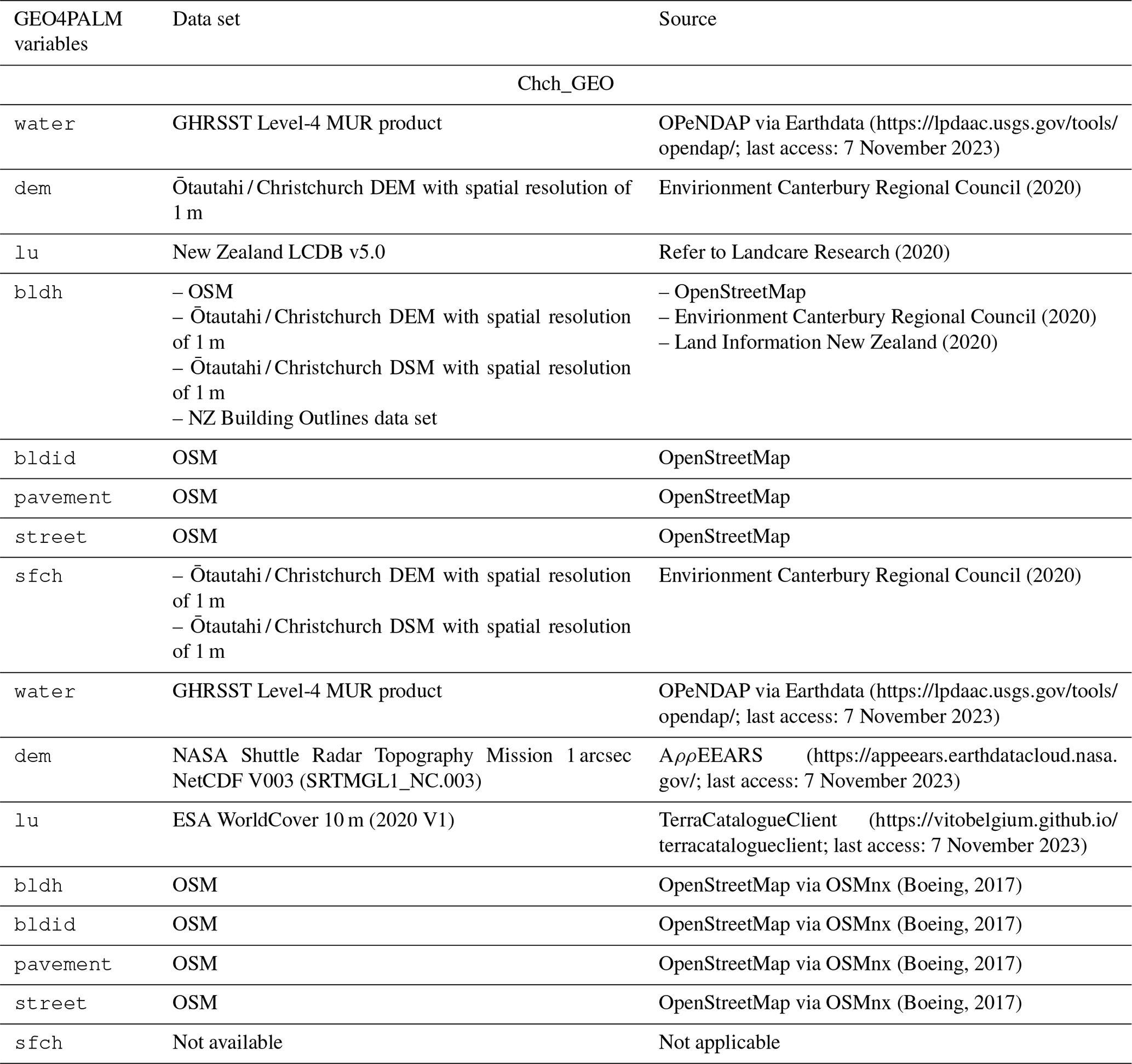
In this section, we present a case study for Ōtautahi / Christchurch, New Zealand, to demonstrate the application of GEO4PALM when the simulation location changes. Local geospatial data sets are used to demonstrate the suitability and applicability of GEO4PALM for the case Chch_GEO. Similarly to Berlin_OL, Chch_OL used all geospatial data downloaded by GEO4PALM rather than local data sets. PALM CSD was used for Ōtautahi / Christchurch using the same input as Chch_GEO, with the geospatial input files pre-processed into a specific NetCDF format. The input data for this case study are listed in Table 6. The water temperature was obtained from the GHRSST data sets for both simulations. For Chch_GEO, the DEM was obtained from the Envirionment Canterbury Regional Council (2020); the land use classification was obtained from New Zealand LCDB v5.0 (Landcare Research, 2020); the building footprint, location, and building ID were derived using OSM data and the NZ Building Outlines data set (Land Information New Zealand, 2020); the building height was calculated using the difference between the DSM and DEM at the building locations; the pavement and street data were obtained from OSM and converted to PALM-recognisable data using the conversion provided by Heldens et al. (2020); and the tree height was derived using the difference between the DSM and DEM with buildings excluded.

Envirionment Canterbury Regional Council (2020)Landcare Research (2020)Envirionment Canterbury Regional Council (2020)Land Information New Zealand (2020)Envirionment Canterbury Regional Council (2020)(Boeing, 2017)(Boeing, 2017)(Boeing, 2017)(Boeing, 2017)

Table 6 Geospatial input data for GEO4PALM used in the Ōtautahi / Christchurch case study.

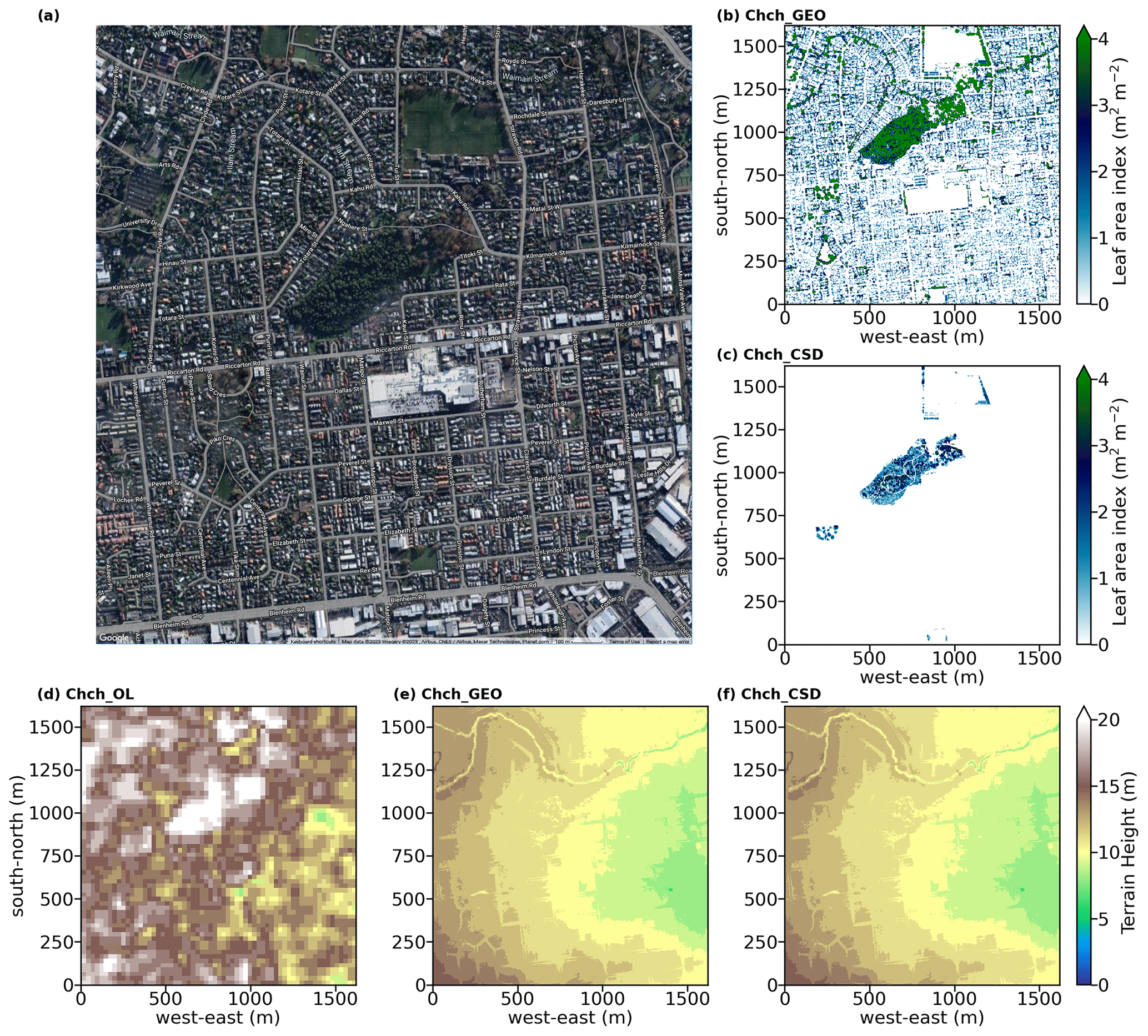
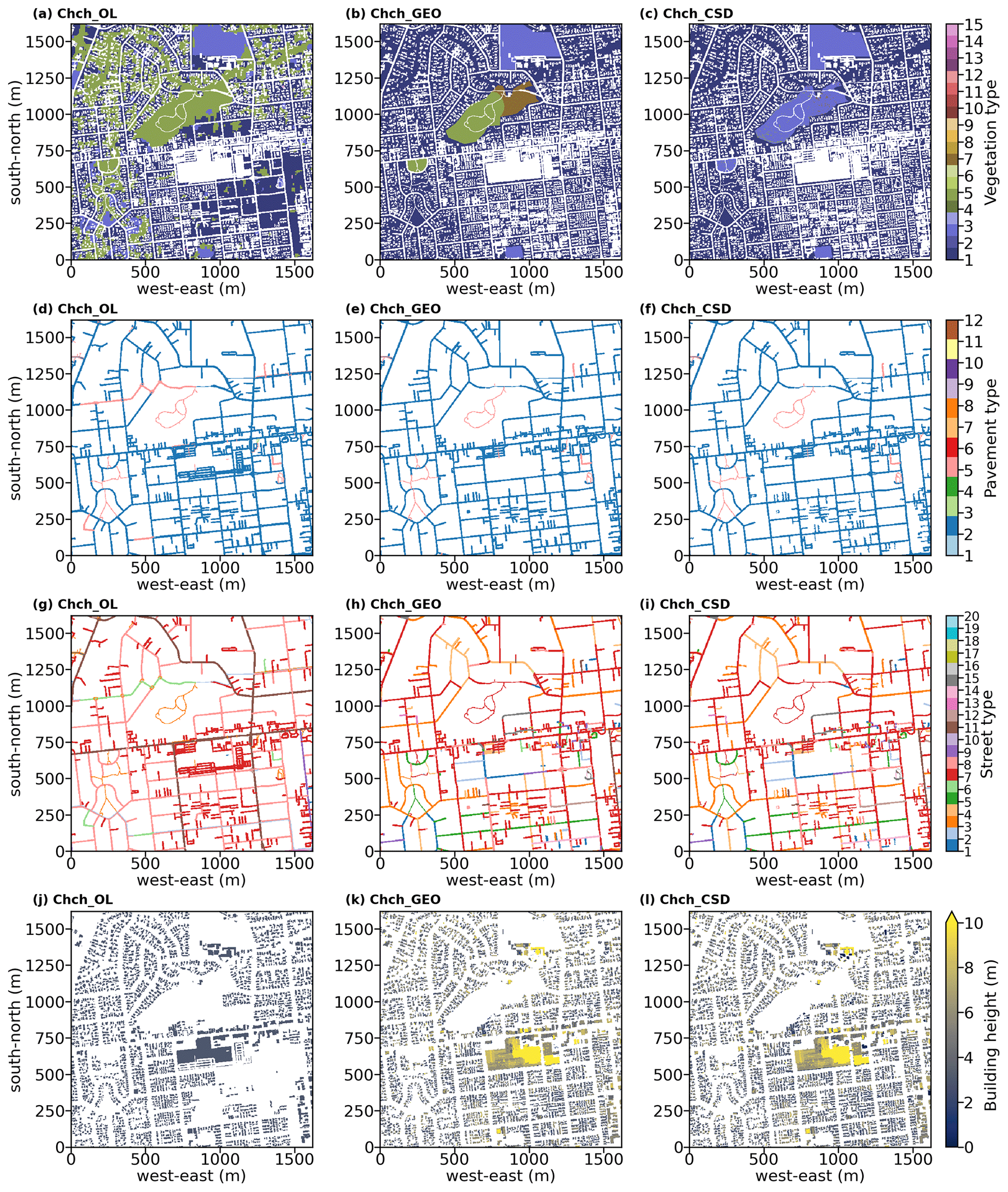
Figures 9 and 10 show the domain location and static input data for the nested domain of 3 m grid spacing (domain N03) for Chch_OL, Chch_GEO, and Chch_CSD. Riccarton Bush is located near the centre of domain N03, with sports fields to its north and Westfield Riccarton (the largest building in the domain) to its south. Riccarton Bush coincides with high LAI over an area of approximately 98 000 m², as shown in Fig. 9b. Again, due to the coarse resolution of the online DEM data, Chch_OL does not present good details of topography height (Fig. 9d) compared to Chch_GEO (Fig. 9e). However, Chch_OL does capture the decrease in topography from west to east of the domain. It should be noted that the NASA topography data may have included surface objects' heights (compare Fig. 9d to Fig. 9e–f), while the DEM and topography in the concept of GEO4PALM and PALM refer to the topographical height only. Users should take extra care if they use the NASA topography data. As the New Zealand land use data set (New Zealand LCDB v5.0) classifies all urban area as only one type, most of the area within the city of Ōtautahi / Christchurch was identified as bare soil by GEO4PALM (Fig. 10b). This is different in the ESA WorldCover data set where Chch_OL shows more areas with vegetation type 5 (deciduous needleleaf trees; green in Fig. 10a), which aligns with the satellite image shown in Fig. 9a. Pavement type and street type are almost identical in Chch_OL (Fig. 10d and g) and Chch_GEO (Fig. 10e and h) as they both used OSM data. The OSM data used in Chch_OL may be more up to date, while Chch_GEO used local data that were processed and checked manually. In GEO4PALM, the OSM interface recognised the footpath on the Westfield Riccarton rooftop car park as pavements. GEO4PALM removes the buildings if they overlap with pavements, whereas PALM CSD removes the pavements when they overlap with buildings. More investigation is needed to determine a more appropriate overlap check. However, in this case, the removal of buildings could be problematic. Comparing Fig. 10j to Fig. 10k, Chch_OL has several buildings missing. Since Chch_GEO was sourced from both OSM and the NZ Building Outlines data set (Land Information New Zealand, 2020), its building information is more comprehensive and accurate. In addition, similarly to the Berlin case, OSM online data do not provide much building height information, and hence, most buildings in Chch_OL have a dummy height of 3 m (Fig. 10j).

Using the same input files, the static driver input created by GEO4PALM and PALM CSD are almost identical. The LAI input for PALM CSD is derived using the LAI calculated by GEO4PALM. In other words, the LAI shown in Fig. 9c for Chch_CSD used the LAI shown in Fig. 9b for Chch_GEO as an input. Since PALM CSD applies adjustments to the vegetation type (see Fig. 10b–c) and checks the resolved plant canopy and its underlying vegetation types, the LAI in Chch_CSD is only present over areas where the vegetation type is not bare soil (see Fig. 9c).

Figure 9 Similar to Fig. 4 but for the Ōtautahi / Christchurch case. Domain centre is located near Riccarton Bush in Ōtautahi / Christchurch, New Zealand (satellite image © Google Earth). Refer to the panel label for the corresponding simulation. For data sources refer to Table 6.

Figure 10 Similar to Fig. 5 but for the Ōtautahi / Christchurch case. Refer to the panel label for the corresponding simulation. For data sources refer to Table 6.

Simulation results for the Ōtautahi / Christchurch case are shown in Figs. 11, 12, and 13. Similarly to the Berlin case, due to the coarse resolution of the input topography data, Chch_OL presents results with box-like structures, especially over the sports fields to the north of Riccarton Bush, where the land is exposed with no surface objects like buildings and plant canopies. The impact of the plant canopies is noticeable in Chch_GEO and Chch_OL. In contrast to Chch_OL, Chch_GEO presents lower θ_2m (Fig. 11a–f) and T_sfc (Fig. 11g–l) over the plant canopies. Compared to Chch_CSD, the different configuration of vegetation types in Chch_OL introduces a warm bias in θ_2m (Fig. 11a–b) and a cold bias in T_sfc (Fig. 11g and h) over the areas which Chch_OL recognises as vegetation rather than bare soil. The area with missing buildings in Chch_OL is colder than that in Chch_CSD (Fig. 11a–b). Over the Riccarton Bush area, Chch_OL does not have a resolved plant canopy, which leads to an overestimation of T_sfc in the area in the last hour of the simulations (Fig. 13f), while most areas of the domain coincide with a cold bias in T_sfc compared to Chch_CSD. In addition to the missing plant canopy, the lack of building heights leads to a significant overestimation of WS_10 m in Chch_OL in the second and the last hours of the simulations (Fig. 13i–j). The problem of lacking plant and urban canopies is more evident for R_net in Chch_OL. As shown in Fig. 13m, the differences in R_net are positive where the buildings and the resolved plant canopies are not present in Chch_OL. In the last simulation hour, Chch_OL gives a positive bias in R_net for most areas of the domain (Fig. 13n). These results, again, highlight the importance of accurate input geospatial data.

Comparing Chch_GEO to Chch_CSD, the resolved plant canopy plays a major role in the differences between the simulations. The presence of a denser plant canopy over Riccarton Bush in Chch_GEO leads to a cold bias in θ_2m and T_sfc in both the second and the last simulation hours (Fig. 13c–d and g–h). In the second simulation hour, with more resolved plant canopies in the simulation domain, Chch_GEO gives a higher θ_2m and a lower T_sfc (Fig. 13c and g). In the last simulation hour, the impact of plant canopies on θ_2m is significant in that the colder areas in Chch_GEO (Fig. 13d) align with the high-LAI areas shown in Fig. 9b. The increase in surface roughness due to the presence of the denser plant canopies in Chch_GEO also introduces a considerable decrease in wind speed compared to Chch_CSD (Fig. 13k–l). In addition, the R_net in Chch_GEO is generally lower across the entire simulation domain than that in Chch_CSD (Fig. 13o–p). The differences between Chch_GEO and Chch_CSD agree with the assumption that, without the vegetation-type adjustment and with a potentially overestimated LAD, the simulation will create biases, especially in the simulated winds. These differences are evident in the Ōtautahi / Christchurch case because of low buildings and a higher proportion of the resolved plant canopies. In the Berlin case, the tallest building is 123.6 m with a domain-averaged building height of 23.9 m. The highest building in the Ōtautahi / Christchurch case is only 25.0 m high, and the domain-averaged building height is 4.8 m, while most of the trees in Riccarton Bush are over 12.0 m high. Therefore, in the Ōtautahi / Christchurch case, the vegetation is the main surface forcing, and such forcing could alter the simulation results significantly.

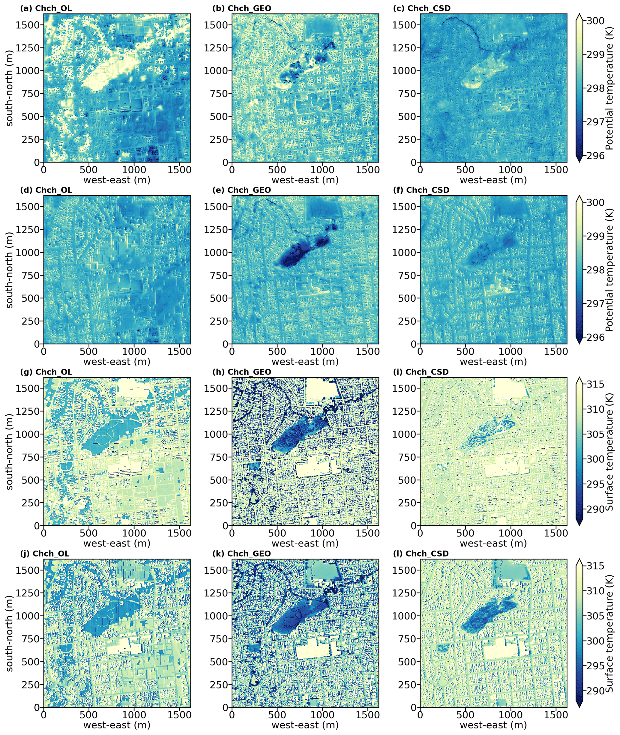
Figure 11 Similar to Fig. 6 but for the Ōtautahi / Christchurch case. Refer to the panel label for the corresponding simulation.

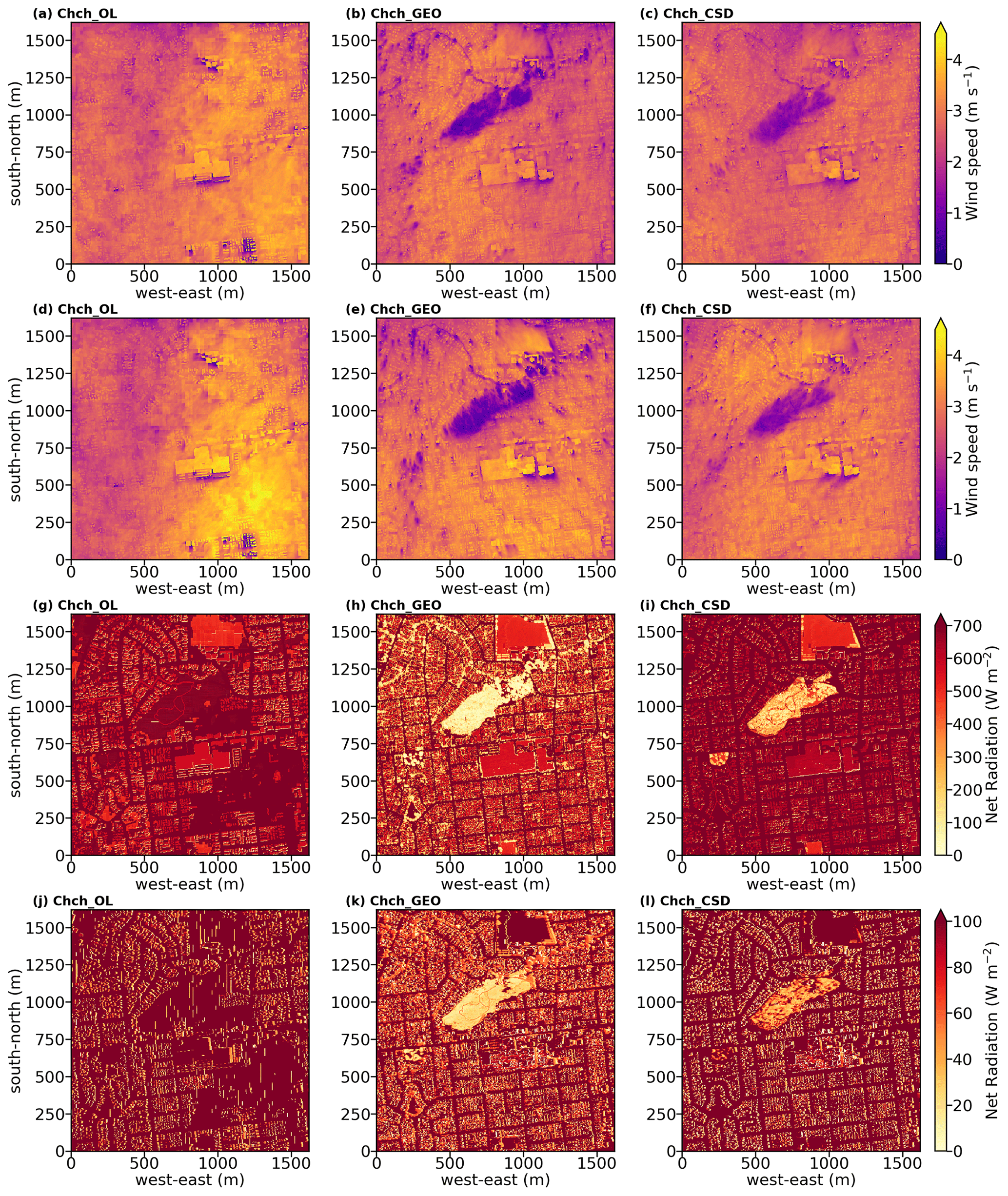
Figure 12 Similar to Fig. 7 but for the Ōtautahi / Christchurch case. Refer to the panel label for the corresponding simulation.

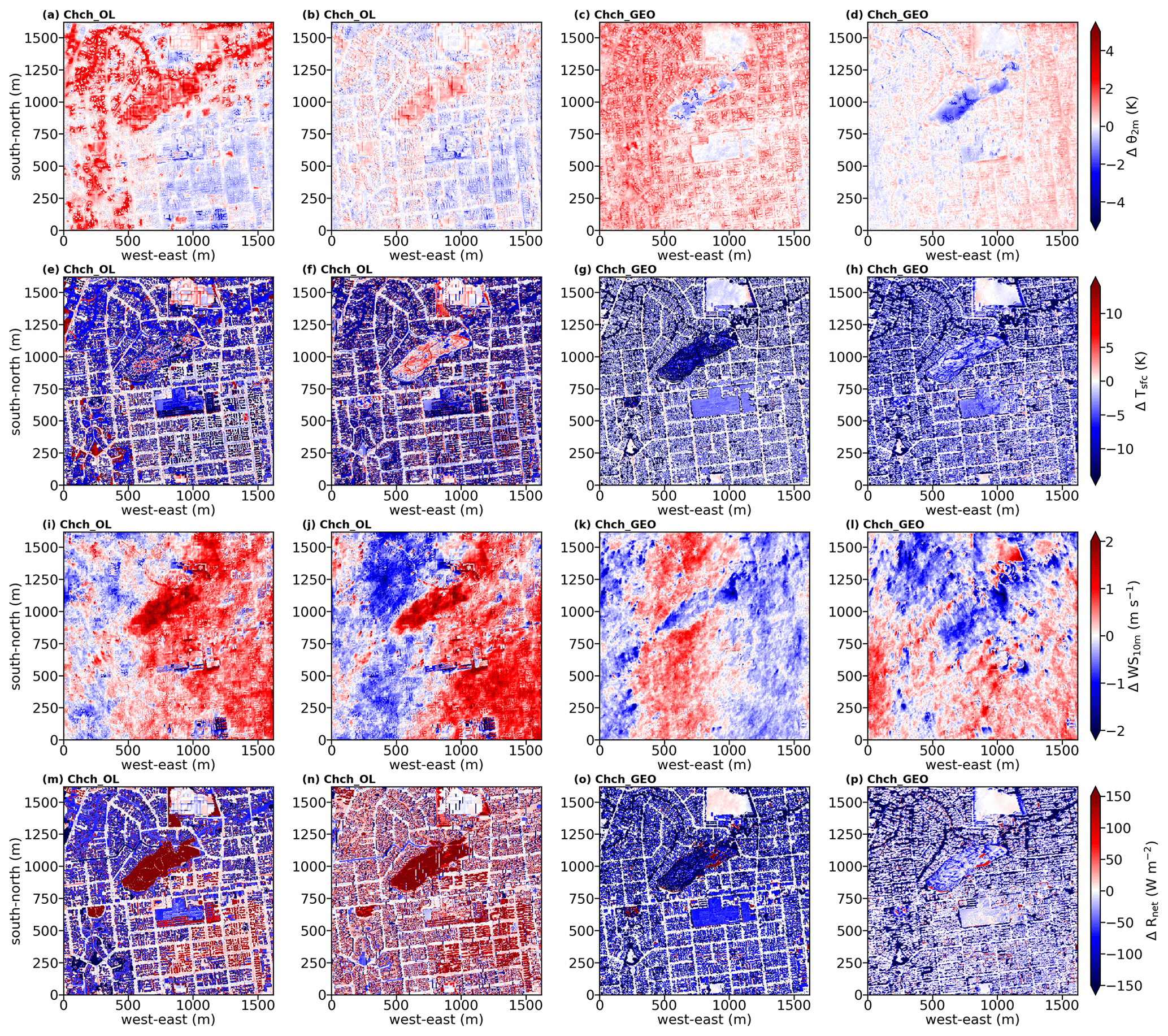
Figure 13 Similar to Fig. 8 but for the Ōtautahi / Christchurch case. Refer to the panel label for the corresponding simulation.

5 Conclusions

This study presents GEO4PALM, a utility written in Python that generates PALM static driver input for the PALM model system. With GEO4PALM, PALM users now have the freedom to create static drivers with any geospatial data they have and/or the online data provided. Two application examples were given to demonstrate the applicability of GEO4PALM. The results show that GEO4PALM is a useful tool to realise near-surface microscale structures. When the same geospatial input data are used, the GEO4PALM static drivers can present simulation results comparable to the PALM CSD static drivers. There are differences between the results generated by the two tools. However, without validations against observational data, we cannot verify which tool's approach is more appropriate. The optimal simulation setup needs to be investigated in future simulations and experiments along with observational data. To the best of our knowledge, current static driver generation tools in the PALM community (PALM CSD, palmpy, and PALM-4U GUI) either heavily rely on users to pre-process geospatial data or have not been applied to many regions in the world, for example, New Zealand. GEO4PALM simplifies data acquisition by automating and standardising data pre-processing and conversion. The online data interfaces, automatic projection conversion, and translation of land cover classes make GEO4PALM a widely applicable tool. These features, however, have not yet been implemented in PALM CSD. In addition to the static driver generation code, GEO4PALM provides a GUI for users to visualise and configure the simulation domains easily.

5.1 Limitations

GEO4PALM is developed as a free, open-source, and community-driven tool and is distributed on GitHub (https://github.com/dongqi-DQ/GEO4PALM; last access: 7 November 2023). As discussed, GEO4PALM does not cover all the variables in the static driver of the PALM model system. The fidelity and features of static driver input depend on the input geospatial data quality and availability, which have been a particular challenge when conducting microscale simulations. GEO4PALM provides several interfaces for users to download global geospatial data sets, which include the basic features of PALM static input, such as topography and land use typology. However, as shown in the case studies, these online data sets are of coarse resolution and are not suitable for high-resolution urban applications at the metre scale. These online data sets could be handy for quickly conducting simulations over a large area with coarse resolutions. The building height and plant canopy information are currently missing in the online data sets covered by GEO4PALM. The LAD estimation method in GEO4PALM may lead to biases in simulations for highly vegetated areas. High-resolution building-type and water temperature data sets are currently not included in GEO4PALM, while these data sets are not publicly available. In addition, GEO4PALM does not apply any adjustments to vegetation types and/or topography. Whether the adjustments would improve the simulations requires further investigation, which is out of the scope of this paper but should be considered in future developments of GEO4PALM.

5.2 Outlook

Many regions worldwide do not have high-resolution geospatial data to realise simulations with high fidelity. High-resolution building height data are important for urban applications, but they are not widely available, making simulations over human settlement difficult. While building height information could sometimes be obtained from the local authorities in large cities, the availability of such data sets might vary depending on the regions of interest. Additionally, for research purposes, there might be differences in accessibility and cost, particularly in smaller or less developed areas. Fortunately, with increasing efforts towards research at the microscale, especially urban climate research, new data sets have been developed for microscale simulations. For example, high-resolution geospatial data can be obtained from Geoscape (https://geoscape.com.au/; last access: 7 November 2023) for applications in Australia. Microsoft provides AI-assisted building footprint mapping (https://www.microsoft.com/en-us/maps/building-footprints; last access: 7 November 2023). Using a deep neural network, the GLObal Building heights for Urban Studies (GLOBUS) gives a novel Level of Detail-1 (LoD-1) building data set (Kamath et al., 2022). Esch et al. (2022) presented World Settlement Footprint 3D, which provides three-dimensional morphology and density of buildings worldwide. Some of these data sets are not freely available or need to be acquired based on individual requests, while GEO4PALM accepts all geospatial data in GeoTIFF format. Once users have obtained the data sets they desire, GEO4PALM is able to process such data for PALM simulations.

Another common challenge in land use data sets is that many land use classification data sets only classify urban areas into a limited number of typologies. This could lead to a loss of fidelity. Lipson et al. (2022) have described a data transformation method to make the urban land use data more descriptive. This may potentially improve the quality of land use classification data sets, for example, for applications in New Zealand, where only one type of land use was classified for urban areas. GEO4PALM currently only accepts vegetation heights as input for plant canopy due to a lack of geospatial data. In the future, we aim to improve this feature based on the PALM CSD tool (Heldens et al., 2020) and to include more data sources if available. While PALM CSD applies various checks on and modifications of the input geospatial data, e.g. topography and vegetation types, these features have not yet been implemented in GEO4PALM. As shown in the Ōtautahi / Christchurch case study, the vegetation-type adjustments could substantially impact the simulation results. Furthermore, this paper only compared GEO4PALM to PALM CSD, while palmpy and PALM-4U GUI are other tools that could have more advanced features. Hence, in addition to the investigation and development of vegetation-type adjustment, future work may also include a comparison between the four tools for better improvements to GEO4PALM.

GEO4PALM accepts any geospatial data sets as input and is easily adaptive to new data downloading interfaces. With the development of geospatial data sets towards better spatial coverage and data quality, GEO4PALM can be improved and extended. All PALM users are encouraged to provide feedback and report bugs and issues via the issue system provided by GitHub. Any optimisation of, modification of, or contribution to the code is welcome and much appreciated.

Appendix A: GEO4PALM step-by-step guide

A more detailed user manual is available at https://github.com/dongqi-DQ/GEO4PALM (last access: 7 November 2023).

A1 Step 1: prepare configuration file

The configuration file should be provided in the ./JOBS/case_name/ folder as follows:

[case]
case_name         -  name of the case
origin_time       -  date and time at model start*
default_proj      -  default is EPSG:4326. This projection uses lat/long to
                     locate domain. This may not be changed.
config_proj       -  projection of input .tif files. GEO4PALM will automatically assign
                     the UTM zone if not provided.
                     We recommend users use local projection with units in metres;
                     e.g. for New Zealand users, EPSG:2193 is a recommended choice.
lu_table          -  land use lookup table to convert land use classification
                     to PALM recognisable

[settings]
water_temperature      -  user input water temperature values when
                          no water temperature data are available
building_height_dummy  -  user input dummy height for buildings
                          where building heights are missing in the
                          OSM data set or if building heights are
                          0.0 m in the input data
tree_height_filter     -  user input to filter small objects; i.e., if
                          object height is smaller than this value,
                          then this object is not included in the LAD estimation

[domain]
ndomain           -  maximum number of domains, when >=2, domain nesting is enabled
centlat, centlon  -  centre latitude and longitude of the first domain. Note this is
                     not required for nested domains
nx                -  number of grid points along the x axis
ny                -  number of grid points along the y axis
nz                -  number of grid points along the z axis
dx                -  grid spacing in metres along the x axis
dy                -  grid spacing in metres along the y axis
dz                -  grid spacing in metres along the z axis
z_origin          -  elevated terrain mean grid position in metres
                     (leave as 0.0 if unknown)
ll_x              -  lower-left corner distance to the first domain in
                      metres along x axis
ll_y              -  lower-left corner distance to the first domain in
                     metres along y axis

[geotif]          -  required input from the user; can be provided by users
                     in the INPUT folder or "online"
water               -  input for water temperature
dem               -  digital elevation model input for topography
lu                -  land use classification

resample_method   -  method to resample GeoTIFF files for interpolation/extrapolation

# if NASA API is used format in YYYY-MM-DD
# SST date should be the same as the orignin_time

## No need to change start/end dates for NASA SRTMGL1_NC.003
dem_start_date = '2000-02-12',
dem_end_date = '2000-02-20',
## start/end dates for land use data set
lu_start_date = '2020-10-01',
lu_end_date = '2020-10-30',

[urban]           - input for urban canopy model; can leave as "" if this
                    feature is not included in the simulations, or provided by
                    users or online from OSM
bldh              - input for building height
bldid             - input for building ID
pavement          - input for pavement type
street            - input for street type

[plant]           - input for plant canopy model; can leave as "" if this
                    feature is not included in the simulations,
                    or provided by users
tree_lai_max      - input value for maximum leaf area index (LAI)
lad_max_height    - input value for the height where the leaf area density (LAD)
                     reaches LADm
sfch              - input for plant height; this is for leaf area density (LAD)

A2 Step 2: provide input files where applicable

Move all input geospatial data to the ./JOBS/case_name/INPUT folder.

A3 Step 3: run the main script

    python run_config_static.py case_name

Appendix B: Land use type lookup table

Table B1 Lookup table to convert NASA LC_Type01 classes to PALM vegetation type, pavement type, building type, water type, and soil type.

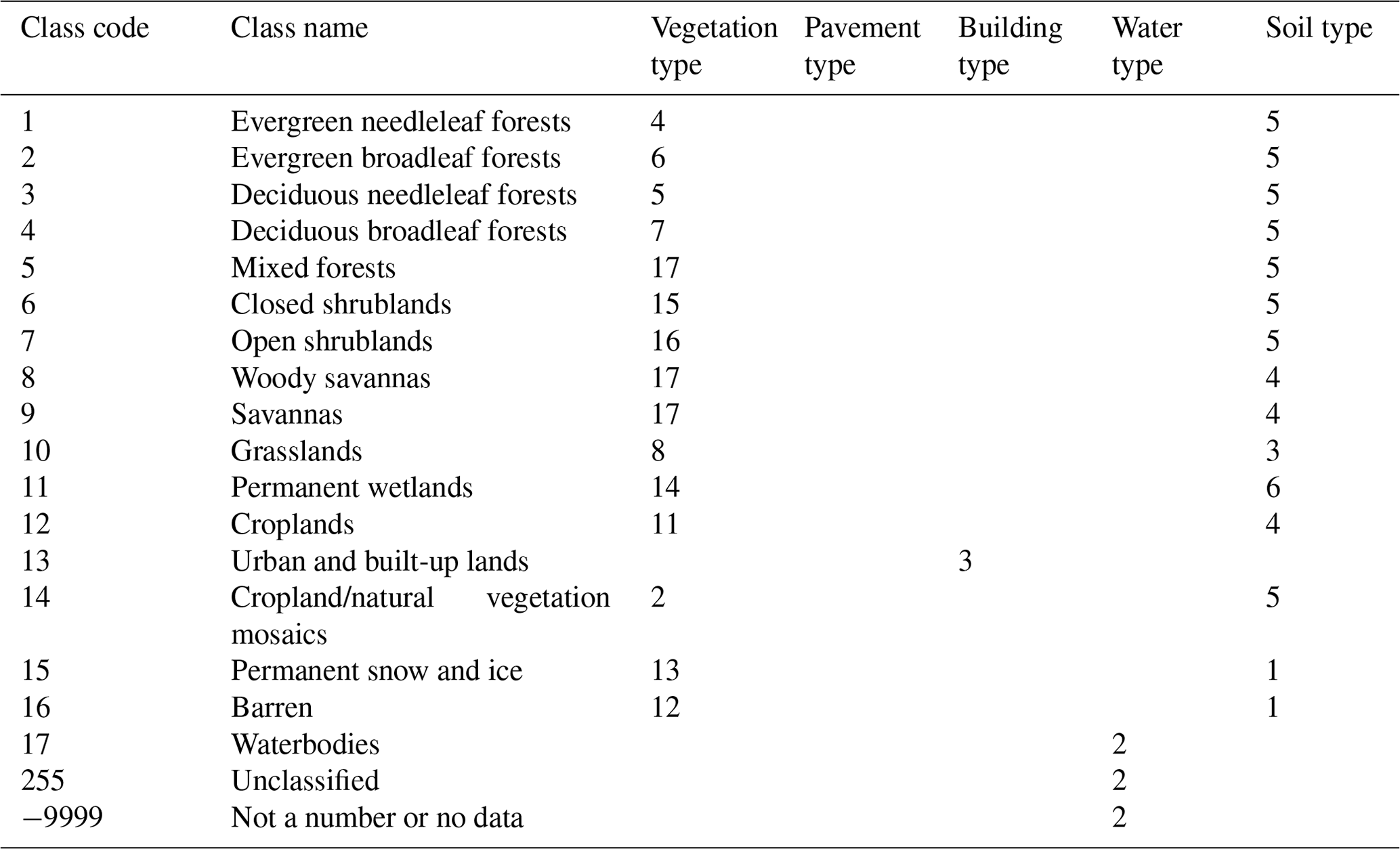
Table B2 Lookup table to convert ESA WorldCover classes to PALM vegetation type, pavement type, building type, water type, and soil type.

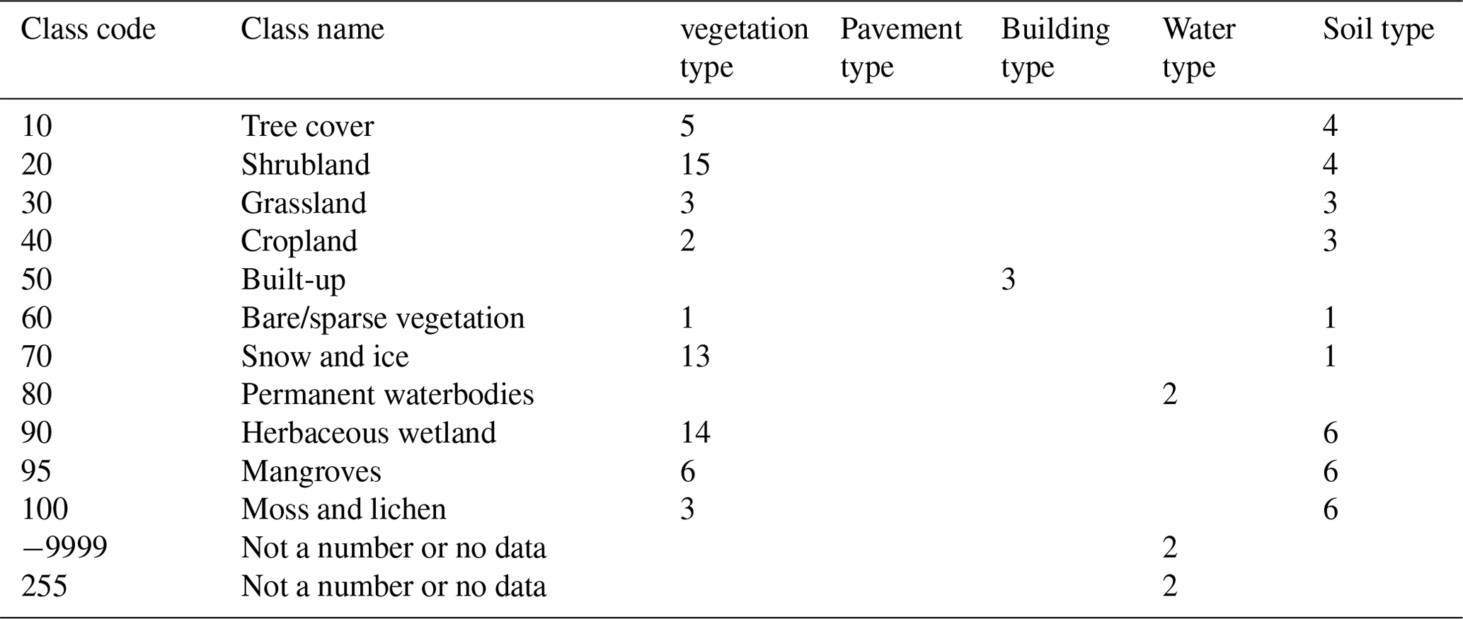
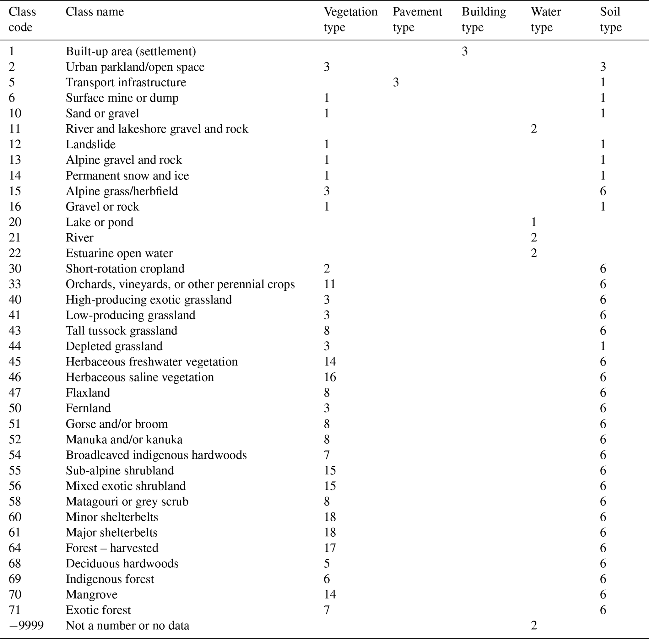
Table B3 Lookup table to convert NZ LCDB v5.0 classes to PALM vegetation type, pavement type, building type, water type, and soil type.