Coupling the regional climate model ICON-CLM v2.6.6 to the Earth system model GCOAST-AHOI v2.0 using OASIS3-MCT v4.0

Interactions and feedback between components of the Earth system can have a significant impact on local and regional climate and its changes due to global warming. These effects can be better represented by regional Earth system models (RESMs) than by traditional stand-alone atmosphere and ocean models. Here, we present the RESM Geesthacht Coupled cOAstal model SysTem (GCOAST)-AHOI v2.0, which includes a new atmospheric component, the regional climate model Icosahedral Nonhydrostatic (ICON)-CLM, which is coupled to the Nucleus for European Modelling of the Ocean (NEMO) and the hydrological discharge model HD via the OASIS3-MCT coupler. The GCOAST-AHOI model has been developed and applied for climate simulations over the EURO-CORDEX domain. Two 11-year simulations from 2008 to 2018 of the uncoupled ICON-CLM and GCOAST-AHOI give similar results for seasonal and annual means of near-surface air temperature, precipitation, mean sea level pressure, and wind speed at a height of 10 m. However, GCOAST-AHOI has a cold sea surface temperature (SST) bias of 1–2 K over the Baltic and North seas that is most pronounced in the winter and spring seasons. A possible reason for the cold SST bias could be the underestimation of the downward shortwave radiation at the surface of ICON-CLM with the current model settings. Despite the cold SST bias, GCOAST-AHOI was able to capture other key variables well, such as those mentioned above. Therefore, GCOAST-AHOI can be a useful tool for long-term climate simulations over the EURO-CORDEX domain. Compared to the stand-alone NEMO3.6 forced by ERA5 and ORAS5 boundary forcing, GCOAST-AHOI has positive biases in sea ice fraction and salinity but negative biases in runoff, which need to be investigated further in the future to improve the coupled simulations. The new OASIS3-MCT coupling interface OMCI implemented in ICON-CLM adds the possibility of coupling ICON-CLM to an external ocean model and an external hydrological discharge model using OASIS3-MCT instead of the YAC (Yet Another Coupler). Using OMCI, it is also possible to set up a RESM with ICON-CLM and other ocean and hydrology models possessing the OASIS3-MCT interface for other regions, such as the Mediterranean Sea.

1 Introduction

GCOAST (Geesthacht Coupled cOAstal model SysTem) is an Earth system framework developed at Helmholtz-Zentrum Hereon, Germany (Staneva et al., 2018). GCOAST is a modular system of different models, each developed for a specific component of the Earth system. Based on a specific scientific question, different models from GCOAST can be selected. These models can be plugged together by various couplers, such as OASIS3-MCT (Craig et al., 2017), ESMF (Earth System Modeling Framework; Hill et al., 2004), or FABM (Framework for Aquatic Biogeochemical Models; Bruggeman and Bolding, 2014). The coupling can be done at different levels of coupling granularity, and the couplers handle the exchange of information between model combinations, individual models, and processes.

GCOAST systems have been applied for several studies covering the Baltic and North Sea region and part of the North Atlantic. These studies include atmosphere–river–ocean–sea ice coupling (Ho-Hagemann et al., 2020), atmosphere–wave coupling (Wahle et al., 2017; Wiese et al., 2019, 2020), wave–ocean coupling (Staneva et al., 2016; Schloen et al., 2017; Lewis et al., 2019), hydrosphere–biosphere coupling for the Elbe estuary (Pein et al., 2019), the total organic carbon–macrobenthos coupling model (Zhang et al., 2019, 2024), and multi-model couplings developed by Lemmen et al. (2018), which have been applied to assess the ecosystem impacts of offshore wind farms (Slavik et al., 2019).

So far, the atmospheric model component of GCOAST has been the non-hydrostatic limited-area atmospheric model COSMO-CLM v5.0 (Rockel et al., 2008). COSMO (COnsortium for Small-scale MOdeling) was initially developed by the Deutscher Wetterdienst (DWD, the German Meteorological Service) in the 2000s as a limited-area weather forecast model. Later, it was developed further in the Climate Limited-area Modeling Community (CLM-Community) as the regional climate model COSMO-CLM (hereafter referred to as CCLM). In December 2021, COSMO v6.0 was released, which is the last version of the COSMO model. With this release, the development of the COSMO model ended after more than 2 decades. The successor of the COSMO model is the Icosahedral Nonhydrostatic (ICON) model.

In 2001, a collaboration between the DWD and the Max Planck Institute for Meteorology (MPI-M) was initiated, with the aim of developing a new modelling system for weather prediction and climate simulations. As one result of this initiative, the global numerical weather prediction model ICON was developed (Zängl et al., 2015). Nowadays, with contributions from the Karlsruhe Institute of Technology (KIT) and the German Climate Computing Center (DKRZ), the ICON Earth system framework includes not only the atmospheric, land, river routing, ocean and sea ice, wave, and biogeochemical compartments but also the Aerosols and Reactive Trace gases (ART) model. ICON can be set up to operate on several high-performance computing systems, such as Bull ATOS at DKRZ (Hamburg, Germany), NEC-Aurora Tsubasa at the DWD (Offenbach, Germany), or BullSequana at Forschungszentrum Jülich (FZJ, Jülich, Germany). ICON can be used on a wide range of scales from climate projection, climate prediction, and numerical weather prediction down to large-eddy simulations (Dipankar et al., 2015; Heinze et al., 2017).

The atmospheric component of ICON includes two different physics packages: the first one is the Numerical Weather Prediction physics package of the DWD (i.e. the ICON-NWP model), and the second one is the ECHAM physics package of the MPI-M (i.e. the ICON-A model, Giorgetta et al., 2018). The global atmospheric model ICON-A is coupled to the global ocean model ICON-O (Korn, 2017) and the land and biosphere model JSBACH (Reick et al., 2021) within the ICON Earth System Model (ICON-ESM; Jungclaus et al., 2022). ICON-NWP can also be coupled to ICON-O in the ICON-Seamless Earth system coupling framework, which has been newly developed in recent years. In ICON-Seamless, there are two options for the land surface schemes, TERRA and JSBACH, which are coupled via subroutines to the atmospheric component. A new land surface model (ICON-Land) is being developed based on JSBACH and some features of TERRA. Another component of ICON-Seamless is the wave model ICON-Wave. The hydrological discharge model HD can now be used as an external model instead of being coupled as a subroutine of JSBACH.

The components of ICON are coupled using YAC (Yet Another Coupler; Hanke et al., 2016). However, coupling between ICON components or coupling of multiple ICON components to an external model without a YAC coupling interface is not supported due to the manner how the initial communicator splitting is implemented.

ICON can also be used in a configuration with regional grid refinement (two-way nesting) or in limited-area mode. ICON-LAM is the limited-area mode of ICON-NWP. Starting in 2017, the DWD and CLM-Community decided to develop the climate limited-area mode (ICON-CLM, Pham et al., 2021) based on ICON-LAM. Within ICON-Seamless, a limited-area mode of the ocean model (ICON-O-LAM) is being developed and can be coupled to ICON-LAM via YAC.

As mentioned above, coupling a component or multiple components of ICON to an external model that has no YAC coupling interface is not supported and is potentially impossible. For the coupling of ICON-CLM as an atmosphere component to GCOAST-AHOI, which includes HD and the ocean model NEMO (Nucleus for European Modelling of the Ocean, Madec et al., 2017) representing the ocean and sea ice components, basically there were two feasible options: either implement a YAC interface in NEMO and HD or implement an OASIS interface in ICON-CLM. For the first option, the YAC coupling interface was added to the HD source code by Moritz Hanke (DKRZ) (see Hagemann et al., 2023), but YAC is not yet available in the NEMO source code. To the best of our current knowledge, there is no RESM with NEMO using YAC. NEMO is already linked to the OASIS coupler, which has been used to couple NEMO to many other model components. Implementing the YAC interface in NEMO would require a larger effort, as the NEMO source code is much more complicated than the HD code. In addition, although the NEMO source code is freely available, we are ordinary users in the NEMO community, not members of the model development team. Therefore, implementing and especially maintaining the YAC interface in NEMO is a big challenge. For the second option, HD and NEMO already have the OASIS3-MCT coupling interface (OMCI), so all we had to do was implement OMCI in ICON. Here, we also have the advantage that we belong to the ICON development team of CLM-Community, so we can get great and quick technical support from the development team when coding with ICON. Therefore, in 2021, we started to port the OASIS coupling interfaces from CCLM to ICON-CLM for coupling to NEMO and HD.

Some other groups were using a similar method while coupling ICON to their available coupled system model which did not include YAC. For example, Bauer et al. (2021) implemented the ESMF interfaces in an earlier version of ICON-NWP as well as in the ocean General Estuarine Transport Model (GETM) to build up the regional ocean–atmosphere coupling over the Baltic Sea. However, they did not consider sea ice in the coupling. There is ongoing work at FZJ to couple ICON-CLM to the Community Land Model (CLM) via the OASIS3-MCT coupler (manuscript in preparation), as has been done for the CCLM via the OASIS interface (Shrestha et al., 2014; Will et al., 2017).

The aim of this article is to give a detailed description of the OASIS3-MCT coupling interface (hereafter referred to as OMCI) in ICON-CLM (ICON release version 2.6.6), how to implement OMCI with as little modification of the ICON source code as possible, how to compile it on the high-performance computing system Levante at DKRZ, and how to run the coupled system model GCOAST-AHOI with ICON-CLM for climate simulations over the EURO-CORDEX domain. This information is useful to other groups planning to couple ICON-CLM to NEMO or any other ocean model that already has an OASIS3-MCT interface available. The Earth system modelling (ESM) community agrees that ICON and IFS (coupled to FESOM and NEMO) will play a central role in the Helmholtz Association of German Research Centres (HGF). This new OMCI opens more opportunities to use ICON-CLM in ESM applications as well as in other modelling communities. OMCI can also be applied for coupling to a land surface model with minor necessary adaptations.

We briefly introduce the coupled system model GCOAST-AHOI in Sect. 2 and give the details of OMCI in ICON-CLM in Sect. 3. The experiment setups are presented in Sect. 4, followed by an analysis of the model simulations in Sect. 5. Finally, conclusions and a discussion are given in Sect. 6.

2 The coupled system model GCOAST-AHOI

GCOAST-AHOI is a subset of GCOAST that includes model components for A-Atmosphere and Land, H-Hydrological discharge, O-Ocean, and I-Sea Ice. GCOAST-AHOI version 1.0 (Ho-Hagemann et al., 2020) contains the atmospheric model CCLM v5.0, the ocean model NEMO3.6 (including the sea ice model LIM3), and the hydrological discharge model HD v4.0 (Hagemann and Dümenil, 1998; Hagemann et al., 2020), coupled via OASIS3-MCT v2.0. A detailed description of CCLM, NEMO, and HD as components of GCOAST-AHOI can be found in Ho-Hagemann et al. (2020).

In GCOAST-AHOI v2.0, ICON-CLM replaces CCLM as the atmospheric model, which is coupled to NEMO3.6 and HD v5.1 via OASIS3-MCT v4.0. By coupling the atmosphere–ocean–river runoff models in GCOAST-AHOI, we aim to close the water balance in the RESM. Figure 1 illustrates the three models exchanging radiation, wind, pressure, temperature, humidity, water, and sea ice variables at their interfaces via the OASIS coupler.

The OMCI in NEMO3.6 has been modified compared to the original one in the officially released version at http://forge.ipsl.jussieu.fr/nemo/wiki/Users/release-3.6 to be able to receive state variables from the atmospheric model (Ho-Hagemann, 2024). Supplement Sect. S1 contains a flowchart of the OMCI for NEMO3.6. This flowchart differs slightly from Fig. 9 in Will et al. (2017), who used the older version (NEMO v3.3). The OMCI in HD can be found in the source code publication of Hagemann and Ho-Hagemann (2021) and Hagemann et al. (2023). Section S2 in the Supplement shows the OMCI of HD. In this article, we describe in detail the OMCI in ICON-CLM.

In Sect. 3, we demonstrate the construction of the OMCI in ICON-CLM and the optional coupling methods between ICON-CLM and NEMO.

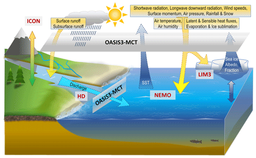
Figure 1 Model components of GCOAST-AHOI and variables exchanged via the OASIS3-MCT coupler. Two solid arrows display the communication between the atmosphere and land (yellow-green arrow) and between the ocean and sea ice (grey-blue arrow), which is done via subroutines inside ICON-CLM and NEMO, respectively. Dotted arrows show the transfer between components via the OASIS interface. Yellow arrows present atmospheric transfer to ocean sea ice and river runoff. The cyan arrow shows the discharge from the river to the ocean. Blue arrows demonstrate the transfer of sea surface temperature (SST) from the ocean as well as the sea ice albedo and sea ice fraction to the atmosphere.

3 The OASIS3-MCT coupling interface in ICON

3.1 Interface structure

Figure 2 shows a flowchart of ICON with the OMCI implemented for coupling to NEMO and HD. Ten levels of ICON's source code are described: the first level is the main program ICON, the second level starts with start_mpi, then comes atmo_model, and the code ends with stop_mpi.

Levels 2 to 6, 8, and 9 comprise subroutines of ICON (marked in red) that are modified by the coupling. At levels 3 to 7 and 10, new subroutines (orange boxes B1–B7) have been added with the OMCI. They are organized into three modules (cpl_oas_vardef.f90, cpl_oas_mpi.f90, and cpl_oas_interface.f90) containing about 3000 lines of Fortran code (including the current debug lines). The files have been added to the icon/externals/oasis3-mct directory and linked to the src/atm_phy_nwp directory of the ICON source tree. The detailed description of the interface structure can be found in Sect. S4 in the Supplement.

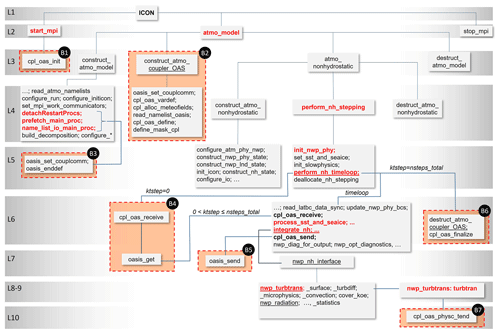
Figure 2 Flowchart of ICON-NWP/ICON-CLM with the OASIS3-MCT coupling interface OMCI. The running sequence is from top to bottom and from left to right. “L1” indicates Level 1 – main program ICON. At levels 2 to 6, 8, and 9, subroutines (in red text) of ICON are modified by the coupling. At levels 3 to 7 and 10, subroutines added for OMCI are shown in orange boxes (B1–B7).

Supplement Sect. S5 contains a guide for compiling ICON with this OMCI on Levante at DKRZ. The preparation of OASIS input files for GCOAST-AHOI is described in Supplement Sect. S6, which is accompanied by an example of the namcouple file in Supplement Sect. S7 and namelist_cpl_atm_oce in Supplement Sect. S8. The command to run GCOAST-AHOI on Levante is provided in Supplement Sect. S9. The complete package to conduct experiments for this study is included in the Starter Package for ICON-CLM Experiments (SPICE; Rockel and Geyer, 2022), which is a workflow engine to easily perform long-term simulations. This tool has been developed further from the ICON-CLM_SP starter package (Pham et al., 2021). Some additional parts for coupling to NEMO and HD have been added to the original package.

3.2 Coupling methods

In the officially released NEMO3.6, several fluxes and variables, including shortwave (SW) and longwave (LW) radiation fluxes, latent heat (LH) and sensible heat (SH) fluxes, rain, snow, evaporation, ice sublimation, mean sea level pressure (MSLP), and surface momentum, can be sent from an atmospheric model to NEMO via the OASIS3-MCT coupler. To be able to receive state variables from the atmospheric model, the OMCI in NEMO3.6 has been modified to allow air temperature and air specific humidity at a height of 2 m (T_2M and QV_2M, respectively) to be sent from the atmospheric model to NEMO. This allows NEMO to use these variables to calculate the LH and SH, as in the case of the stand-alone NEMO using the “CORE bulk formulae” (Large and Yeager, 2004). Thus, we have three options for the coupling method between ICON and NEMO:

• a.

  CPL_flx is for flux coupling, which is the default option in the NEMO source code (described above).

• b.

  CPL_var is for state variable coupling, the new method, where SW and LW, T_2M, QV_2M, wind speed at a height of 10 m (UV_10M), rain, snow, MSLP, and surface momentum are sent from ICON-CLM to NEMO. NEMO calculates LH and SH using the CORE bulk formulae, which are based on the Monin–Obukhov similarity theory.

• c.

  CPL_mix is for mixture coupling, a new method like CPL_var, but ICON-CLM also sends LH and SH to NEMO. NEMO then averages them with the LH and SH calculated using the CORE bulk formulae.

With the modification of OMCI in NEMO3.6, it is now easy to select the coupling method via the namelist settings. Section 5 considers the simulations using coupling method 3 (CPL_mix), which was also used in Ho-Hagemann et al. (2020). An extra experiment using coupling method 1 (CPL_flx) is also conducted and analysed in Sect. 5.

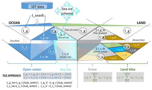
In turn, NEMO sends the sea surface temperature, sea ice fraction, and sea ice albedo to ICON-CLM. Figure 3 illustrates how the surface temperature is updated in ICON over the ocean (left side) and over land (right side) in the presence of sea ice and snow. ICON utilizes a tile approach to compute surface fluxes of momentum and scalars. For the “seawater type” grid boxes, the grid box mean fluxes are computed as a weighted average of the fluxes over ice and over open water, using the fractional ice cover (fice) and the fractional open water cover (1 – fice) as the respective weights. The sea ice in each ICON grid box is considered only if fice exceeds its minimum value of 0.015. Otherwise, the grid box is treated as ice-free. In ICON, two types of surface temperature are considered: the ground temperature t_g and the surface temperature t_s. If a grid box is covered by sea ice or snow, t_g is the mixed temperature of the free sea ice or free snow surface temperature and the temperature on top of the sea ice or snow. Under the sea ice, t_s is calculated as a mixture of the free sea ice temperature and the salt water freezing temperature of 271.45 K. If there is no sea ice or snow in the grid box, t_g is equal to t_s. In principle, NEMO can send the mixed sea ice and water temperature to ICON to update t_g over the ocean points, as in CCLM in Ho-Hagemann et al. (2020). Alternatively, it can send the open water temperature, the sea ice surface temperature, and the sea ice fraction so that ICON can calculate t_g as the mixture. However, in the uncoupled mode of the current ICON-CLM version, the sea surface temperature (SST) forcing is read in as the variable t_seasfc (or t_s_w in Fig. 3) and passes through the subroutines nwp_ surface_init and process_sst_and_seaice to calculate t_g. To be consistent with the ICON-CLM updates, we pass the SST (to update t_seasfc), the sea ice fraction (to update fr_seaice), and the sea ice albedo (alb_si_ext) from NEMO to ICON. ICON will then calculate t_g, t_s, alb_si, etc., using its sea ice scheme. In the future, we may modify this coupling method by using the sea ice temperature from NEMO.

Figure 3 Surface temperature exchange between the atmosphere and ocean or land in ICON and GCOAST-AHOI.

4 Experimental design

In this study, four main experiments are conducted for the period 2008–2018 (Table 2): the uncoupled ICON (ICON266), the coupled GCOAST-AHOI (ICPL266), the stand-alone NEMO v3.6 (NEMO3.6), and the stand-alone HD v5.1 forced by ICON266 runoffs (HDICON266). Two additional experiments are conducted: ICPL266_noNewa as a sensitivity test for the location of the Newa River mouth on the NEMO grid and ICPL266_flx to test the coupling method CPL_flx.

Table 1 Model configuration.

Table 2 Model experiments.

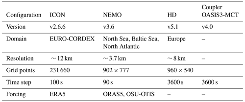
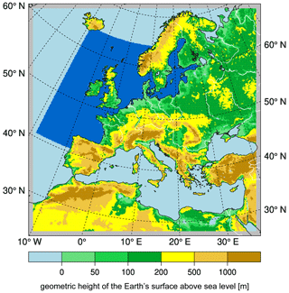
Each experiment starts on 1 January 2008 and ends on 1 January 2019, restarting each month. The integration domains of ICON, NEMO, and HD are displayed in Fig. 4. The namelist setup of physical parameterization for ICON-CLM is similar to that of the NUKLEUS project (Beate Geyer, personal communication, May 2023). The resolution of ICON is R13B5, with an approximate mesh size of 12 km using 60 vertical levels. The model top height is 23.5 km. The following physical schemes are used in the current namelist setting of ICON: the radiation scheme ecRad (Hogan and Bozzo, 2018; Rieger et al., 2019), mass-flux shallow and deep convection scheme (Tiedtke, 1989; Bechtold et al., 2008), microphysics single-moment scheme (Doms et al., 2021), planetary boundary layer scheme with prognostic TKE (Raschendorfer, 2001; Raupach and Shaw, 1982), and land surface scheme tiled TERRA (Schrodin and Heise, 2001; Schulz et al., 2016; Schulz and Vogel, 2020). The initial and lateral boundary forcing of ICON is obtained from the ERA5 reanalysis data (Hersbach et al., 2020). The Tegen aerosol climatology (Tegen, 1997), i.e. a monthly aerosol optical depth of sulfate droplets, total dust, organic carbon, black carbon, and sea salt, is used in this study. The initial and daily lateral boundary forcing of NEMO is taken from the ORAS5 reanalysis data (Copernicus Climate Change Service, 2021). The spatial resolution of NEMO is ∼ 3.7 km, with 50 vertical levels. In the stand-alone mode, NEMO3.6 is driven by the atmospheric ERA5 data, the ocean ORAS5 data, and climatological river runoff data. The tidal harmonic forcing for NEMO is derived from the TPXOv8 model (OSU-OTIS, Egbert and Erofeeva, 2002). It is reconstructed for each model time step from the tidal constituents M2, S2, N2, K2, K1, O1, Q1, P1 and M4. HD has a resolution of 1/12°, i.e. ca. 8 km. More information on the model configuration can be found in Table 1 and in Ho-Hagemann et al. (2020).

Figure 4 Integration domains of ICON and HD (EURO-CORDEX) and of NEMO-LIM3 (dark blue).

To estimate the computational performance of the coupled model, we used LUCIA (Maisonnave and Caubel, 2014), which is part of OASIS3-MCT. In Sect. S10 and Fig. S1 in the Supplement, we describe how to use LUCIA for GCOAST-AHOI to optimize the computational performance.

Figure 5 Seasonal (DJF, MAM, JJA, SON) and annual (ANN) means of the sea surface temperature (K) bias of (a) ICPL266, (b) ICPL266_flx, and (c) NEMO3.6 with respect to the OSTIA data for the period 2010–2018 over the GCOAST domain.

5 Evaluation of model simulations

The first 2 years, 2008–2009, are excluded as the spin-up time, and the output data of the two simulations ICON266 and ICPL266 for 9 years (2010–2018) are compared to the observational and ERA5 reanalysis data to assess the model performance. For SST, we use the Operational Sea Surface Temperature and Ice Analysis (OSTIA) data (Good et al., 2020) to evaluate the simulated SST of ICPL266. For air temperature at a height of 2 m (T_2M) and precipitation (TOT_PREC), the daily E-OBS data (Haylock et al., 2008; Van den Besselaar et al., 2011) version 27.0 on a grid of 0.1° are used. The ERA5 reanalysis data are interpolated onto the E-OBS grid and used as a reference for comparison with the simulated shortwave and longwave surface radiation, turbulent fluxes, MSLP, wind speed at a height of 10 m (SP_10M), and T_2M. The Surface Radiation Data Set – Heliosat (SARAH) – Edition 2 (Pfeifroth et al., 2017) is used to evaluate the shortwave downward radiation of the simulations.

Seasonal means of winter (DJF), spring (MAM), summer (JJA), and autumn (SON) and annual means (ANN) of several variables are analysed in this section.

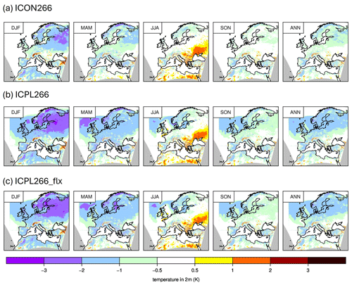
Figure 6 Seasonal (DJF, MAM, JJA, SON) and ANN means of 2 m air temperature (K) differences of (a) ICON266, (b) ICPL266, and (c) ICPL266_flx from the ERA5 reanalysis data for the period 2010–2018.

5.1 Sea surface temperature and 2 m air temperature

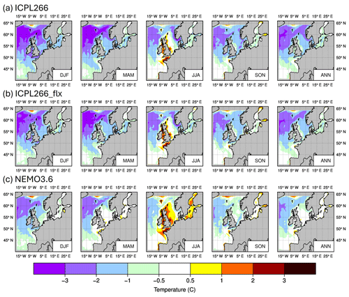
Over the ocean, the SST of ICON266 is the ERA5 forcing data, which are based on observations, so they are very close to the OSTIA data (not shown). Thus, the SST difference between the coupled and stand-alone ICON-CLM simulations (Fig. S2 in the Supplement) can be interpreted as a bias towards a measurement-based product. In the coupled model, the SST is provided by NEMO over the GCOAST domain. In general, ICPL266 has a cold SST bias of about 1–3 °C compared to OSTIA over the GCOAST domain, except around the coast of the United Kingdom in summer (JJA, Fig. 5a). The SST bias of ICPL266_flx (Fig. 5b) is similar to that of ICPL266 (Fig. 5a). Ho-Hagemann et al. (2020) noted that using CPL_flx when coupling COSMO-CLM to NEMO leads to larger biases in the SST than using CPL_mix. This is not the case here when coupling ICON-CLM. A possible reason for this is that, due to the tile approach (see Sect. 3.2), the fluxes from ICON-CLM to NEMO are sent separately over water and sea ice, while COSMO-CLM v5.0 does not use the tile approach. Therefore, the fluxes in each ocean grid box sent from the atmosphere to the ocean are the mixed fluxes of water and sea ice.

The annual mean SST bias of the stand-alone NEMO3.6 is less than 0.5 °C over the Baltic and North seas and about −1 to −2 °C over the North Atlantic compared to the OSTIA data (Fig. 5c). In summer, a positive SST bias of about 1–2 °C is present over the Baltic and North seas. In this case, the reduction in SST by the coupling reduces the warm bias of the stand-alone NEMO3.6.

The cold SST bias of ICPL266 over the GCOAST domain intensifies the cold T_2M bias (Figs. 6b, S2b in the Supplement), especially in winter (DJF) and spring (MAM). In summer, ICPL266 reduces the warm T_2M bias of ICON266 (Fig. 6a). In general, the ANN T_2M bias of ICPL266 is slightly more negative, by about 0.5 °C, than that of ICON266. ICPL266_flx reproduces a similar T_2M (Fig. 6c) to that of ICPL266. Comparison with the E-OBS data (Fig. S3 in the Supplement) shows similar results to Fig. 6, except over northern Africa and Türkiye, where the quality of the E-OBS data is affected by the lack of observations in that region (see Fig. 1 in Hagemann and Stacke, 2022).

5.2 Shortwave radiation, longwave radiation, and turbulent fluxes

A possible reason for the SST cold bias of ICPL266 may be that the shortwave and longwave radiation from ICON-CLM sent to NEMO is too low. Figure S4 in the Supplement shows the relative bias (%) of the shortwave downward radiation (SWDN) of ICON266 and ICPL266 compared to the ERA5 data, together with the relative difference (%) between SARAH2 and ERA5. Figure 7 shows a zoomed section of Fig. S4 over the GCOAST ocean domain (note the adapted colour scale). In general, both ICON266 and ICPL266 have a positive SWDN bias of less than 10 % over land compared to ERA5, except for the larger bias of 15 %–20 % over northern Europe in winter and eastern Europe in autumn (Fig. S4). Over the North Sea, ICON266 and ICPL266 have a small negative bias of about 5 %–10 % compared to ERA5 (Fig. 7). The area of negative SWDN bias in the North Sea is slightly larger in ICPL266 than in ICON266. Comparing the ERA5 data and the SARAH2 data, the SWDN over southern Europe is similar between the two datasets, with SARAH2 being slightly larger over land (Fig. S4). In general, the SWDN of ICON266 and ICPL266 over the North Sea is rather close to the SARAH2 data but is slightly overestimated over the Baltic Sea.

Figure S5 in the Supplement shows a similar plot to Fig. S4 but for the longwave downward radiation (LWDN) and without the SARAH2 data, as they are not available. The modelled LWDN has a negative bias of about 2 %–4 % annually and a larger bias in winter of about 6 %–8 % that is most pronounced over land. Over the ocean, ICON266 reproduces the LWDN of the ERA5 data well, and ICPL266 has a small negative bias of 2 %–4 %. Overall, the negative SWDN bias over the North Sea and the negative LWDN bias of ICON-CLM give an indication of why ICPL266 shows an increased cold SST bias.

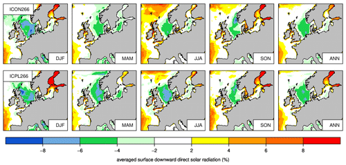
Figure 7 Seasonal (DJF, MAM, JJA, SON) and ANN means of the shortwave downward radiation bias (%) of ICON266 (top) and ICPL266 (bottom) compared to the ERA5 data for the period 2010–2018 over the GCOAST domain.

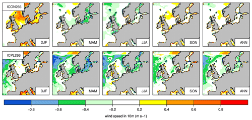
Figure 8 Seasonal (DJF, MAM, JJA, SON) and ANN mean 10 m wind speed bias (m s⁻¹) of ICON266 (top) and ICPL266 (bottom) compared to the ERA5 data for the period 2010–2018 over the GCOAST domain.

The ERA5 reanalysis data are used as the atmospheric forcing for the uncoupled NEMO3.6, and the namelist settings of NEMO used in this study were tuned for an SST close to OSTIA (Fig. 5c). If the same namelist settings of NEMO3.6 are used for ICPL266, to reduce the cold SST bias over the North Sea in the coupled simulations, a bias correction for SWDN and LWDN should be done. Figures S6a, b and S7a, b in the Supplement show the seasonal SWDN and LWDN of ICPL266 and NEMO3.6 averaged over the North Sea and Baltic Sea for the period 2010–2018. Note that we do not show the result of ICPL266_flx in Figs. S6 and S7 because there is no output of LWDN in ICPL266_flx due to the setup of the CPL_flx coupling method. Over the North Sea, the SWDN of ICPL266 is smaller than that of ERA5 used for NEMO3.6 in spring and summer (Fig. S6a), which mainly leads to the cold SST bias of ICPL266 (Fig. 5a). Therefore, we plan to increase the SWDN of ICON by about 10 % before sending it to NEMO. However, the cold SST bias over the Baltic Sea does not seem to be directly related to the SWDN as there is no clear SWDN difference between ICPL266 and NEMO3.6 in summer or in any other season (Fig. S6a). The LWDN of ICPL266 is similar to that of NEMO3.6 in summer but slightly smaller in the other three seasons, over both the North Sea and the Baltic Sea. Increasing the LWDN in ICON-CLM by about 5–10 W m⁻² before sending it to NEMO should be tested to reduce the SST bias. Note that the seasonal cycle of the LWDN is more pronounced over the North Sea than over the Baltic Sea.

We also compare the turbulent heat flux (i.e. the sum of SH and LH) of NEMO3.6 and the flux of NEMO in ICPL266, averaged over the North Sea and the Baltic Sea (Figs. S6c and S7c), and the net downward heat flux, which is the sum of SWDN, LWDN, SH, and LH (Figs. S6d and S7d). We only consider the turbulent flux because NEMO does not write out SH and LH separately, but only the SWDN, LWDN, and net downward heat flux. Note that the turbulent flux from NEMO3.6 is calculated using the CORE bulk formulae and, due to the CPL_mix coupling method used, the turbulent flux in NEMO from ICPL266 is the average of the flux from ICON-CLM and the one calculated inside NEMO (see Sect. 3.2). The results are similar for both seas. The turbulent flux and the net downward flux of the two experiments are quite similar, with the largest differences in winter (DJF) and summer (JJA).

Using ERA5 as a reference, the SH and LH biases of ICON266 and ICPL266 are shown in Figs. S8 and S9 in the Supplement. Over land, the bias of ICON266 is very similar to that of ICPL266. However, over the ocean, the bias of ICPL266 is generally more positive (i.e. the fluxes are less negative) than that of ICON266, with the largest bias over the North Atlantic. Smaller heat fluxes are consistent with lower SSTs in ICPL266, as lower SSTs lead to larger stability and less vertical mixing. Over the North and Baltic seas, the SH and LH of ICPL266 are quite close to ERA5. Despite the SST forcing from ERA5, ICON266 has a negative SH bias of about −5 to −15 W m⁻² over the North and Baltic seas, especially in winter. This suggests future analysis of the difference in air temperature at the lowest level of ICON-CLM and ERA5.

Besides the energy flux biases causing the cold SST bias, a spin-up time of 2 years may be too short for NEMO to reach the stable state, leading to the cold SST bias. In addition, NEMO's namelist settings should be optimized for the coupled simulations.

Currently, in the COPAT2 (Coordinated Parameter Testing, phase 2) initiative of CLM-Community, several parameters of ICON-CLM are being tested in a similar way to that done for COSMO-CLM (Russo et al., 2024) to find the recommended settings. For example, the use of the transient aerosol MACv2-SP (Kinne, 2019; Stevens et al., 2017) and a careful adjustment of various namelist settings related to cloud cover, the soil and vegetation scheme, and the turbulent transfer will further reduce the T_2M cold bias and improve the shortwave downward radiation.

Figure 9 Seasonal (DJF, MAM, JJA, SON) and ANN differences of precipitation (millimetres per month) for (a) ICON266, (b) ICPL266, and (c) ICPL266_flx compared to the E-OBS data for the period 2010–2018.

5.3 Precipitation, mean sea level pressure, and wind speed

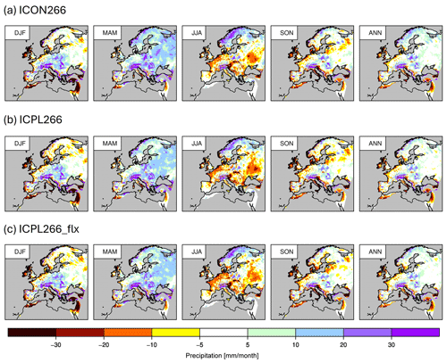
The precipitation biases (Fig. 9) of the three simulations ICON266, ICPL266, and ICPL266_flx compared to the E-OBS data are very similar in general, with a wet bias in winter and spring and a dry bias in summer (JJA) and autumn (SON). Figures S10 and S11 in the Supplement show the biases of MSLP and SP_10M of ICON266 and ICPL266 compared to ERA5. The MSLP and SP_10M figures of ICPL266_flx are not shown because they are very similar to those of ICPL266.

ICPL266 tends to overestimate the MSLP throughout the year, except in summer, while ICON266 only has a pronounced positive bias in winter (DJF) and a negative bias in summer (JJA). The wind speed of the two simulations is very similar over land (Fig. S11). ICPL266 reduces the wind speed over the GCOAST ocean domain by up to 1.5 m s⁻¹ compared to ICON266 (Figs. 8 and S11). Therefore, while ICON266 has a positive bias of about 0.5 m s⁻¹ over the North Sea and the Baltic Sea in winter (Fig. S11a), ICPL266 is very close to ERA5 (Fig. S11b). In general, ICPL266 produces a cooler SST and weaker wind speed than ICON266, which is consistent with the smaller SH mentioned above in Sect. 5.2. This positive feedback is known as the thermal feedback (TFB) mechanism in the atmosphere–ocean surface coupling process (Zhang and Perrie, 2001; Renault et al., 2023).

Figure 10 shows the monthly climatology of different variables (T_S, T_2M, TOT_PREC, and MSLP) over the GCOAST domain or the whole EURO-CORDEX domain, considering only ocean or land points. ICPL266 has a cold T_S bias of about 1–2 °C over the ocean (Fig. 10a), which also causes the T_2M bias of 0.5–1 °C over the ocean (Fig. 10c). In winter, ICPL266 is slightly colder over land than ICON266 and E-OBS (Fig. 10d). In summer, both simulations are very close to E-OBS. The simulated precipitation of ICON266 tends to be overestimated compared to E-OBS, with maxima in May and June, and slightly underestimated in August and September (Fig. 10b). The coupled run shows 1–3 mm less precipitation per month than the atmosphere-only experiment. In previous studies by Ho-Hagemann et al. (2015, 2017), the stand-alone atmospheric model COSMO-CLM has a dry bias in summer and the coupled run reduces the dry bias due to the improvement of the moisture convergence and transport from ocean to land. This situation is not found in the current study, which needs to be thoroughly analysed in the future.

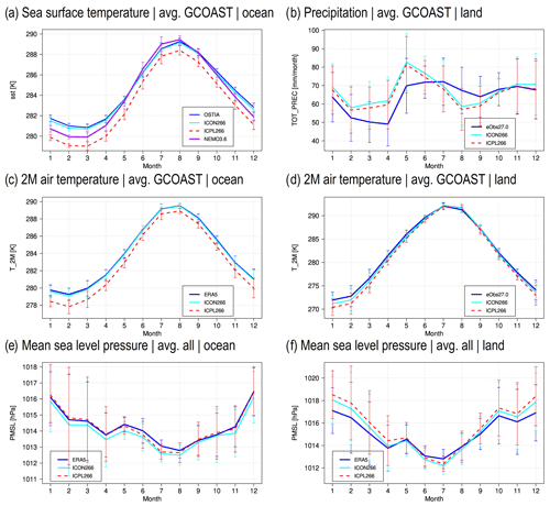
Figure 10 Climatological monthly mean of T_S (K), T_2M (K), MSLP (hPa), and precipitation (millimetres per month) of ICON266 (solid cyan line) and ICPL266 (red dashed line) compared to the OSTIA, ERA5, and E-OBS data (solid blue line) for the period 2010–2018. Panel (a) also includes the SST of NEMO3.6 (solid purple line) averaged over the GCOAST domain. Values are averaged over the GCOAST domain (avg GCOAST), over the whole EURO-CORDEX domain (avg all), over the ocean, or over land points only. The vertical bars show the standard deviation of the area mean data.

For the MSLP, the whole EURO-CORDEX domain is considered, but separately for ocean points (Fig. 10e) and land points (Fig. 10f). In both cases, ICPL266 has a higher MSLP than ICON266. The higher surface pressure in ICPL266 may be caused by the cooler air near the surface (due to the negative T_2M bias), which leads to a higher density of the air mass and therefore a higher pressure. Over the ocean, the MSLP of ERA5 is reproduced better by ICPL266 than by ICON266. Over land, ICPL266 increases the MSLP's positive bias in winter compared to ICON266. ICPL266_flx and ICPL266 have similar results (not shown), indicating that the coupling methods used in GCOAST-AHOI v2.0 do not greatly affect the simulated climate variables in this study.

5.4 Sea ice

The sea ice fraction bias of ICPL266 is about 0.2–0.3 over the Bothnian Bay and Bothnian Sea in winter and spring (Fig. 11a), while ICPL266_flx has a larger bias of about 0.3–0.5 (Fig. 11b) and the ERA5-forced NEMO3.6 has a relatively small positive ice fraction bias there (Fig. 11c). The monthly mean sea ice fraction averaged over the Bothnian Bay and Bothnian Sea from ICPL266 and NEMO3.6 compared to the OSTIA data is shown in Fig. 11d, where the sea ice's temporal variation is captured quite well by the two models, with a high peak in spring 2010 and a low peak in spring 2015. However, all three simulations overestimate the sea ice fraction of OSTIA, with the two coupled simulations also showing a larger positive bias in the time series. While ICPL266 has a winter SWDN about 8 % larger than that of ERA5 (Fig. 7b), the incoming shortwave radiation is relatively small over the high latitudes in winter. Therefore, we do not expect the positive SWDN bias to be the main reason for the overestimation of sea ice. However, the LWDN of ICPL266 is about 10 W m⁻² lower than that of ERA5 (the forcing for NEMO3.6) in winter over the North and Baltic seas (Figs. S6b, S7b), and T_2M is about 3 °C lower than ERA5 over the Scandinavian region surrounding the Bothnian Bay and Bothnian Sea (Fig. 6b). The cold T_2M bias and negative LWDN bias of ICPL266 may explain its positive sea ice fraction bias. The cold air temperature above the sea ice surface often produces more sea ice in winter and spring, especially over an area with water of low salinity, such as the Bothnian Bay and Bothnian Sea. Figure 6c shows the larger T_2M cold bias of ICPL266_flx over the Baltic Sea in spring of about 1 °C more than ICPL266 (Fig. 6b), which is consistent with the larger sea ice fraction bias of ICPL266_flx (Fig. 11b) compared to that of ICPL266 (Fig. 11a).

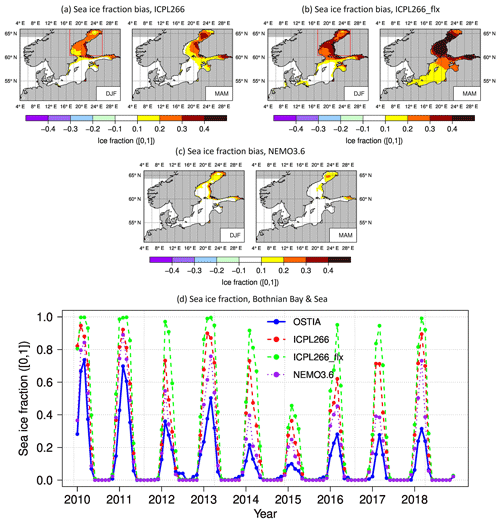
Figure 11 Sea ice fraction bias of (a) ICPL266, (b) ICPL266_flx, and (c) NEMO3.6 compared to the OSTIA data in winter (DJF) and spring (MAM) averaged over the period 2010–2018. (d) Monthly mean of the sea ice fraction averaged over the Bothnian Bay and Bothnian Sea (red box in Fig. 11a) for OSTIA, ICPL266, ICPL266_flx, and NEMO3.6 during 2010–2018.

Another factor that could contribute to an increase in sea ice cover in spring would be an increase in river runoff, which would result in less salty seawater and therefore more sea ice. These two variables are analysed in the next section.

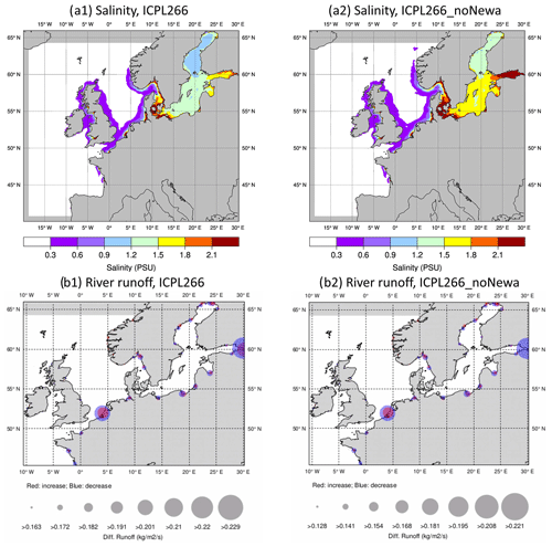
Figure 12 (a1) Salinity difference (PSU) and (b1) river runoff difference (kg m⁻² s⁻¹) between ICPL266 and NEMO3.6 averaged over the period 2010–2018. Panels (a2) and (b2) show the salinity and river runoff difference of ICPL266_noNewa compared to NEMO3.6. In panels (b1) and (b2), the sizes of the grey circles indicate the magnitude of the positive (red) and negative (blue) differences.

5.5 Salinity and river runoff

As mentioned in Sect. 4, NEMO3.6 uses a climatological dataset for river runoff. Therefore, a rough verification of the river runoff produced by the HD model in ICPL266 can be carried out by comparison against this climatological river runoff. Differences in sea surface salinity and river runoff between ICPL266 and NEMO3.6 are shown in Fig. 12. The salinity simulated by ICPL266 is about 0.3–1 PSU higher than that of NEMO3.6 along the United Kingdom and the North Sea coast and about 0.9–1.8 PSU higher in the Baltic Sea. The two areas with the largest salinity differences of more than 2 PSU are found south of the Kattegat and in the Gulf of Finland (Fig. 12a). The river runoff differences (Fig. 12b) are largest near the Ems and Newa estuaries, with more than 0.1 and 0.2 kg m⁻² s⁻¹, respectively. The small river runoff difference between the two models at the Kattegat cannot be used to directly explain the increase in salinity there. The river runoff differences near the Ems estuary have opposite signs (blue point overlaid by a red one in Fig. 12b) but very similar values. The reason for this may be the discrepancy in the locations of river mouths between the NEMO3.6 setup, where the river runoff is taken from a climatology, and those in ICPL266, which are defined based on the river mouths in the HD model and the NEMO land–sea mask. In the latter case, the river mouths of the HD model are interpolated onto the NEMO grid by searching for the closest ocean point of NEMO. For example, the Ems River mouth in ICPL266 may not be in the same position as in the climatology data. This discrepancy would lead to a difference in salinity near the coast (see Fig. 12a). The extent of the effect on salinity in the deeper layers of the ocean in a longer-term simulation needs to be analysed in the future.

The large difference in river runoff near the Newa estuary is also caused by a mismatch in the locations of the river mouths. In this case, the mouth of the Newa River in the climatology data (60.1333° N, 29.888° E) is located slightly north-west of its “real” location (59.9453° N, 30.1708° E). The interpolation program used to define the mouths of the HD rivers on the NEMO grid, by searching for the ocean point closest to the mouths of the HD rivers, found the mouth of the Newa River at 59.95835° N, 30.20825° E, which is very close to the real location and at the furthest grid point to the east in the Gulf of Finland. However, in NEMO, this eastern boundary point in the Gulf of Finland is masked as a buffer zone. Therefore, the discharge from HD to NEMO at this point in ICPL266_noNewa was ignored in the NEMO calculations, resulting in a lack of freshwater inflow to the Gulf of Finland in ICPL266 (Fig. 12b2) and consequently an increase in salinity (Fig. 12a2). The ICPL266 simulation with the Newa River mouth located in the NEMO buffer zone is referred to as ICPL266_noNewa in Fig. 12. To overcome the location deficiency, the Newa River mouth was shifted one grid point to the west on the NEMO grid to allow the large amount of river runoff to enter the Gulf of Finland in the coupled model. Therefore, the salinity difference of ICPL266 compared to NEMO3.6 is reduced (Fig. 12a1), and the river runoff difference shows the shift in the river mouth instead of the missing one (Fig. 12b1). The shift in the Newa River mouth has little effect on the simulated atmospheric variables but improves the simulated salinity in the Baltic Sea, which is important for ecosystem modelling when a marine biogeochemical or ecosystem model such as ECOSMO (Daewel and Schrum, 2013) is coupled to GCOAST-AHOI in the future.

Other river mouths in the Baltic Sea have river runoff differences of less than 1.4 kg m⁻² s⁻¹ when comparing ICPL266 to NEMO3.6. In general, ICPL266 tends to simulate less river runoff than the climatology, leading to increased salinity there. The sources of the river runoff used for NEMO in ICPL266 are the surface and sub-surface runoffs from the land component in ICON-CLM that are transported to the ocean by HD. We applied the HD model to calculate the discharge using the ICPL266 and ICON266 surface and sub-surface runoffs (Table 3) to evaluate it against the discharge observation. The annual discharge difference of ICPL266 and HDICON266 in the Baltic Sea is about −11 %. However, HDICON266 with a discharge of 12 449 m³ s⁻¹ is about −20 % biased towards the HELCOM (Helsinki Commission; Svendsen and Gustafsson, 2022) value of 15 676 m³ s⁻¹. Note that, for Baltic Sea ocean models, the mean long-term bias of river runoff must be less than 7 % (Hagemann and Stacke, 2022). In the North Sea, ICPL266 discharge is about −4 % compared to HDICON266, which has an annual value of 6366 m³ s⁻¹. However, both models have a dry discharge bias compared to the OSPAR data (Farkas and Skarbøvik, 2021), i.e. 9190 m³ s⁻¹.

Table 3 Seasonal discharge (m³ s⁻¹) of ICPL266 and HDICON266 summed over the North Sea and the Baltic Sea during the period 2010–2018. “Diff. (%)” is the difference between ICPL266 and HDICON266.

The main driver of the runoff is precipitation. Figure 9 shows that, over Scandinavia, ICON266 has a wet bias of about 10–30 mm per month in spring and summer compared to the E-OBS data. Thus, even with the wet precipitation bias, ICON266 has a dry discharge bias. At the same time, ICPL266 precipitation is lower than that of ICON266 in spring and summer and therefore is closer to the E-OBS data (Fig. 9b). This difference in precipitation between ICPL266 and ICON266 explains the −11 % difference in discharge, which increases the dry discharge bias. The reduction in the precipitation bias in ICPL266 leading to a larger discharge dry bias implies that a better simulation of precipitation compared to observations does not necessarily lead to a better runoff. We note that the runoff from the atmosphere-only ICON-CLM has a general dry bias, which can be attributed to the respective parameterizations in the TERRA land surface scheme used in ICON-CLM (Stefan Hagemann, personal communication, February 2024). This dry discharge bias can be improved either by using the JSBACH land surface model in ICON-Seamless or by applying a discharge bias correction developed by Hagemann et al. (2024).

In Sect. 5.4, it was speculated that an increase in river runoff would lead to less saline seawater and therefore more sea ice over the Baltic Sea. In our study, ICPL266 simulates too little river runoff, leading to increased salinity in the Baltic Sea, which would mean less sea ice. However, the sea ice fraction is increased compared to the ERA5-forced NEMO3.6. Thus, the main factor causing the bias in the sea ice fraction seems to be the cold bias in the air temperature over sea ice in the Baltic Sea in winter and spring (Fig. 6b and c).

6 Conclusion and outlook

In the present study, we introduce the regional Earth system model (RESM) GCOAST-AHOI v2.0, in which a new atmospheric component – the regional climate model ICON-CLM version 2.6.6 – is coupled to the ocean model NEMO3.6 and the hydrological discharge model HD version 5.1 via the OASIS3-MCT coupler version 4.0.

GCOAST-AHOI v2.0 is developed and applied for climate simulations over the EURO-CORDEX domain. Several 11-year simulations from 2008 to 2018 of the uncoupled ICON-CLM (ICON266) and GCOAST-AHOI (ICPL266, ICPL266_flx, and ICPL266_noNewa) yield similar results for seasonal and annual means of near-surface air temperature and precipitation as well as MSLP and wind speed at a height of 10 m. However, GCOAST-AHOI has a cold SST bias of 1–2 °C over the Baltic and North seas that is most pronounced in the winter and spring seasons. The coupling methods CPL_mix and CPL_flx give similar biases of SST and other climate variables like T_2M, precipitation, or MSLP.

A possible reason for the cold SST bias of GCOAST-AHOI could be the underestimation of the downward shortwave radiation at the surface of ICON-CLM with the current model settings. A deeper analysis of the bias will be done in the next study, especially after re-running the simulations with the optimal settings of ICON-CLM, which will be found in the COPAT2 initiative of CLM-Community. For example, the performance of ICON-CLM will be tuned by using the transient MACv2-SP aerosol data (Kinne, 2019) and modified namelist parameters related to cloud cover to improve the shortwave downward radiation and reduce the cold bias.

Despite the cold SST bias, GCOAST-AHOI was able to capture the distribution of temperature, precipitation, mean sea level pressure, and wind speed well, similar to the uncoupled ICON-CLM. However, GCOAST-AHOI provides larger biases in sea ice fraction and salinity over the Baltic Sea compared to the stand-alone ocean simulation (NEMO3.6) forced by ERA5 and ORAS5. The sea ice fraction bias is related to the cold T_2M bias in ICPL266 and ICPL266_flx. Using the flux coupling method CPL_flx instead of CPL_mix does not greatly affect the bias of SST and climate variables but causes a larger sea ice fraction positive bias over the Baltic Sea. In the future study, a new simulation of ICPL266 with the CPL_var coupling method will be conducted and compared to the current ICPL266 and ICPL266_flx experiments to investigate the impact of the coupling methods on the sea ice simulation.

The salinity bias is attributed to the dry runoff bias of ICPL266 compared to the climatology, with the largest bias values found near the Ems and Newa estuaries. The dry runoff bias near the Ems and Newa mouths is due to a mismatch of the river mouth locations between the climatology and ICPL266. An adjustment of the Newa River mouth location must be made to allow the Newa River runoff to flow into the Gulf of Finland. The effect of the river runoff bias on salinity in the deeper layers of the ocean should be analysed in the future.

In addition, the added value of the coupled model compared to the stand-alone model is usually found in the case of extreme events (Ho-Hagemann et al., 2015, 2017, 2020; Wiese et al., 2019, 2020). Therefore, we will analyse the model simulations with a focus on extreme events in the next study.

Our present study shows that the RESM GCOAST-AHOI can be a useful tool for conducting long-term regional climate simulations. The new OASIS3-MCT coupling interface (OMCI) implemented in ICON-CLM adds the possibility of coupling ICON-CLM to an external ocean model and an external hydrological discharge model, not only with NEMO and HD, using OASIS3-MCT instead of YAC. Given that the stand-alone model components for the atmosphere and the ocean are available for a specific geographical domain, it is also quite easy to apply GCOAST-AHOI to other regions. Besides preparing the lateral boundary conditions for NEMO over the new domain and preparing the OASIS input files (as described in Sects. S6 and S7), it is necessary to prepare several new parameter files so that OASIS3-MCT can exchange the discharge from HD to NEMO without interpolation. On the one hand, these are files for the general setup of the HD model. The creation of these files is described in Sect. 3 of the HD model readme markdown file included in the HD model package (Hagemann et al., 2023). On the other hand, this includes the HD model coupling file, which is used for coupling via OASIS. Instructions for its generation are provided in Sect. 2.1 of a markdown file dedicated to the HD model coupling exercises (Hagemann et al., 2023).

ICON-CLM with OMCI is also used to couple ICON-CLM to NEMO v4.2 over the GCOAST domain (manuscript in preparation) and to NEMO-MED v3.6 over the Mediterranean Sea region in CLM-Community. OMCI for the older ICON version 2.6.4 can be found in Ho-Hagemann (2022).

Recently, the ICON consortium developed and released the Community Interface (ComIn) for the ICON model to allow ICON to be coupled to external model components. The main challenge for the external model component coupling is the initial splitting of MPI_COMM_WORLD, which is done in ICON by a grouping of the MPI communicators (MPI-handshake) (Moritz Hanke, personal communication, July 2024). There are about 40 ComIn entry points in the new release version of ICON. Using the ComIn entry points does not require any additional patching of the ICON source code. A coupling interface to an external model such as OMCI would have to be moved into a ComIn plugin to connect to the entry points in the ICON source code. In addition, the communicator splitting using the MPI-handshake algorithm would have to be implemented in the NEMO and HD source code.

Currently, a limited-area mode of the ocean model (ICON-O-LAM) is also being developed by the ICON consortium. This can be coupled to ICON-CLM via YAC in the ICON-Seamless framework. When that RESM is available in the future and is applied to the EURO-CORDEX domain, its simulation will be able to be compared to the simulations of GCOAST-AHOI as a good reference. Investigating differences in simulations of the two RESMs could be helpful for better understanding the coupling interactions and feedback between model components of the climate system.