Impact of ocean vertical-mixing parameterization on Arctic sea ice and upper-ocean properties using the NEMO-SI3 model

We evaluate the vertical turbulent-kinetic-energy (TKE) mixing scheme of the NEMO-SI3 ocean–sea-ice model in sea-ice-covered regions of the Arctic Ocean. Specifically, we assess the parameters involved in TKE mixed-layer-penetration (MLP) parameterization. This ad hoc parameterization aims to capture processes that impact the ocean surface boundary layer, such as near-inertial oscillations, ocean swells, and waves, which are often not well represented in the default TKE scheme. We evaluate this parameterization for the first time in three regions of the Arctic Ocean: the Makarov, Eurasian, and Canada basins.

We demonstrate the strong effect of the scaling parameter that accounts for the presence of sea ice. Our results confirm that TKE MLP must be scaled down below sea ice to avoid unrealistically deep mixed layers. The other parameters evaluated are the percentage of energy penetrating below the mixed layer and the length scale of its decay with depth. All these parameters affect mixed-layer depth and its seasonal cycle, surface temperature, and salinity, as well as underlying stratification. Shallow mixed layers are associated with stronger stratification and fresh surface anomalies, and deeper mixed layers correspond to weaker stratification and salty surface anomalies.

Notably, we observe significant impacts on sea-ice thickness across the Arctic Ocean in two scenarios: when the scaling parameter due to sea ice is absent and when the TKE mixed-layer-penetration process vanishes. In the former case, we observe an increase of several meters in mixed-layer depth, along with a reduction in sea-ice thickness ranging from 30 to 40 cm, reflecting the impact of stronger mixing. Conversely, in the latter case, we notice that a shallower mixed layer is accompanied by a moderate increase in sea-ice thickness, ranging from 10 to 20 cm, as expected from weaker mixing. Additionally, interannual variability suggests that experiments incorporating a scaling parameter based on sea-ice concentration display an increased mixed-layer depth during periods of reduced sea ice, which is consistent with observed trends. These findings underscore the influence of enhanced ocean mixing, through specific parameterizations, on the physical properties of the upper ocean and sea ice.

1 Introduction

In the last decades, global climate change has strongly affected the Arctic region, leading to a fast decrease in sea-ice extent (Perovich and Richter-Menge, 2009). This phenomenon, together with an increase in openings in the ice pack, modifies the exchanges between the atmosphere and ocean and hence modifies the fully coupled atmosphere–sea-ice–ocean system in the Arctic (McPhee, 2008). These changes have, in turn, led to alterations in the physical properties of the upper ocean, with implications for sea-ice dynamics and response (Lenn et al., 2022). The upper layer of the Arctic Ocean, known as the Arctic mixed layer (ML), plays a pivotal role in regulating interactions between the deeper ocean, sea ice, and the atmosphere. Key factors influencing the Arctic ML include heat, freshwater, and momentum fluxes generated by ocean–atmosphere exchanges, currents, tides, and waves (Rabe et al., 2022; Rudels and Carmack, 2022). Observational data from the past few decades have revealed changes in both winter and summer MLs across the high Arctic, accompanied by changes in ocean stratification (Cole and Stadler, 2019; Peralta-Ferriz and Woodgate, 2015). These rapid transformations of the Arctic environment have far-reaching implications for climate and socioeconomic aspects (Ford et al., 2021). Therefore, achieving an accurate representation of the Arctic Ocean and sea ice in models is essential for understanding and predicting these consequential changes.

Sea-ice–ocean general circulation models used in coupled models assessed by the Intergovernmental Panel on Climate Change (IPCC) (Cassotta et al., 2022) exhibit significant discrepancies in Arctic ML depth (Allende et al., 2023), which are directly influenced by vertical mass and momentum exchanges between the upper ocean and sea ice. These small-scale vertical processes are parameterized in general circulation models. The NEMO-SI3 ocean–sea-ice model (Madec et al., 2017; Vancoppenolle et al., 2023) includes the vertical turbulent-kinetic-energy (TKE) closure scheme initially proposed by Blanke and Delecluse (1993). The scheme is complemented by an additional source of TKE to simulate the effects of near-inertial oscillations, ocean swells, and waves, specifically known as TKE mixed-layer penetration. TKE mixed-layer penetration has been introduced to overcome summer biases in the mixed layer, which was too shallow in the Southern Ocean (Calvert and Siddorn, 2013; Rodgers et al., 2014). The approach redistributes a percentage of surface TKE below the mixed-layer depth. Moreover, TKE mixed-layer penetration is attenuated in the presence of sea ice. Previous research, such as that conducted by Calvert and Siddorn (2013), has emphasized the impact of this parameterization on ocean properties in regions without sea ice. Additionally, Heuzé et al. (2015) have underscored the effect of this parameterization on deep convection in the Southern Ocean. However, the specific influence of TKE mixed-layer penetration below sea ice has not been documented in the literature, although preliminary research carried out within the ArcticMix project (https://marine.copernicus.eu/about/research-development-projects/2016-2018/arcticmix, last access: 18 October 2024) suggests that this influence is large. This is an important issue because the NEMO-SI3 ocean–sea-ice model is extensively used in polar-climate studies (e.g., Goosse et al., 2023; Dong et al., 2023; Docquier et al., 2017; Vancoppenolle et al., 2008) and is featured in the IPCC's assessment reports.

This study aims to evaluate the impact of changes in TKE mixed-layer penetration across three distinct ice-covered regions within the Arctic Ocean: the Makarov, Eurasian, and Canada basins. The Makarov Basin, located north of Siberia, experiences seasonal ice cover and receives freshwater from the East Siberian Sea. Shallow depths (500–1500 m) render it highly sensitive to sea-ice variability and freshwater inputs. The Eurasian Basin extends from the East Siberian Shelf to the North Pole, featuring extensive multi-year ice cover and significant freshwater discharge from major Arctic rivers. Depths can reach 4000 m, influencing Arctic freshwater storage and sea-ice dynamics. The Canada Basin, situated between North America and Siberia, is dominated by multi-year ice influenced by the Beaufort Gyre. Its complex bathymetry, including deep ridges (such as the Alpha and Mendeleev ridges), affects ocean circulation patterns and carbon cycling. Sea-ice and upper-ocean physical properties are closely linked due to mass and momentum exchanges at the ice–ocean boundary, exhibiting seasonal variations. In fall and winter, seawater freezes, and sea ice forms, accompanied by brine rejection. This process involves the rejection of salt from the crystal structure of water ice, increasing salinity in the upper-ocean layer. Consequently, ocean stratification weakens, leading to a deeper ML. In spring and summer, as sea ice melts, freshwater is released into the ocean, reducing salt concentration and strengthening ocean stratification, thereby causing the ML to become shallower. By varying the parameters within this scheme, we illustrate how ocean and sea-ice physical properties respond to alterations in upper-ocean mixing. The paper is organized as follows. Section 2 provides a description of the NEMO-SI3 configuration, parameters, and outputs involved in the study, as well as the oceanic and sea-ice observation data. Section 3 presents a diagnosis of seasonal and interannual variability in upper-ocean and sea-ice properties in three regions of the Arctic Ocean by varying the mixing scheme. Finally, Sect. 4 presents concluding remarks and discusses the implications of our work.

2 Method

The vertical turbulent-kinetic-energy (TKE) closure scheme implemented in NEMO is based on the model developed by Bougeault and Lacarrere (1989) for the atmospheric boundary layer. It was subsequently adapted for an oceanic context by Gaspar et al. (1990) and integrated by Blanke and Delecluse (1993) into the Océan PArallélisé (OPA) model, which is the ocean model component of the NEMO platform. In essence, this TKE closure model provides a prognostic for the evolution of turbulent kinetic energy ($\stackrel{\mathrm{‾}}{e}$) and a closure assumption for turbulent length scales, both necessary for computing vertical eddy viscosity and diffusivity coefficients. The prognostic equation is given by

$$\begin{array}{}\text{(1)}& {\displaystyle \frac{\partial \stackrel{\mathrm{‾}}{e}}{\partial t}}=K_m{\left({\displaystyle \frac{\partial {\stackrel{\mathrm{‾}}{U}}_h}{\partial z}}\right)}^{\mathrm{2}}-K_{\mathit{\rho }}{N}^{\mathrm{2}}+{\displaystyle \frac{\partial }{\partial z}}\left(K_e{\displaystyle \frac{\partial \stackrel{\mathrm{‾}}{e}}{\partial z}}\right)-\mathit{\epsilon }.\end{array}$$

It results from the balance between vertical shear, the dissipation of TKE due to buoyancy, the vertical diffusion of TKE, and energy dissipation. Madec et al. (2017) introduced significant modifications to this parameterization. These changes include considerations such as turbulent-length-scale adjustments that impose an extra assumption regarding the vertical gradient of the computed length scale (Madec et al., 1998). Additionally, a surface wave breaking parameterization has been incorporated, following Mellor and Blumberg (2004), to address the impact of surface wave breaking energetics. The model now accounts for Langmuir cells using a simple parameterization proposed by Axell (2002) for a k–ε turbulent closure. Furthermore, the TKE closure has been updated to include mixing just below the mixed layer. Our study focuses on evaluating the influence of this last modification, which we will refer to as TKE MLP (mixed-layer penetration). This parameterization has been introduced to address the underestimation of ML depth (MLD), especially in situations characterized by windy conditions during the summer months, as observed in the Southern Ocean (Rodgers et al., 2014). This parameterization aims to account for observed phenomena that impact the density structure of the ocean's surface boundary layer. These include near-inertial oscillations, ocean swells, and waves, which are not fully captured by the default TKE scheme. TKE ($\stackrel{\mathrm{‾}}{e}(t,z)$) includes an additional energy source term, ${\stackrel{\mathrm{‾}}{e}}_{\mathrm{inertial}}(t,z)$, which represents the contribution of TKE MLP as

$$\begin{array}{}\text{(2)}& {\stackrel{\mathrm{‾}}{e}}_{\mathrm{inertial}}(t,z)=\left\{\begin{array}{ll}\mathit{\chi }{f}_r{\stackrel{\mathrm{‾}}{e}}_{\mathrm{surf}}{\exp }^{-z/h_{\mathit{\tau }}}& \text{if }z>\mathrm{0}\\ \mathrm{0}& \text{if }z=\mathrm{0}.\end{array}\right.\end{array}$$

Here, z is the depth, and f_r is the fraction of surface TKE (${\stackrel{\mathrm{‾}}{e}}_{\mathrm{surf}}$) that penetrates into the ocean, with values ranging from 0 to a maximum of 0.1. Moreover, h_τ is the vertical-mixing length scale that controls the exponential shape of the penetration. It can be set as a uniform 10 m value, as a latitude-dependent value that varies from 0.5 m at the Equator to 30 m north of 40° latitude, or as different values for the two hemispheres; see Fig. 2 of Storkey et al. (2018). Penetration scales of 10 and 30 m are illustrated in Fig. 1a; 10 m was found to be optimal in the North Pacific (Calvert and Siddorn, 2013), while 30 m was required to improve the ML in the Southern Ocean (Storkey et al., 2018). The degree of this mixing is regulated by the scaling parameter (χ), applied in response to the presence of sea ice. While f_i represents the sea-ice concentration fraction, the parameter χ can take the following values: $\mathit{\chi }=\mathrm{1}-min(\mathrm{1},\mathrm{4}{f}_{\mathrm{i}})$, which is used to suppress the TKE input into the ocean when sea-ice concentration exceeds 25 %; $\mathit{\chi }=\mathrm{1}-\tanh \left(\mathrm{10}{f}_{\mathrm{i}}\right)$, which displays a behavior similar to that of the previous value; or $\mathit{\chi }=\mathrm{1}-f_{\mathrm{i}}$, which decreases linearly as a function of sea-ice fraction. Additionally, the model allows for χ=1, indicating that there is no influence from ice cover.

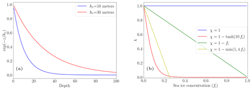
Figure 1 (a) Exponential penetration as a function of depth for two values of the vertical-mixing length scale (h_τ). (b) The scaling parameter (χ) as a function of the sea-ice concentration fraction (f_i) for the four options of the scaling parameter (χ).

To carry out this investigation, we utilize version 4.2 of NEMO (NEMO4.2) using the SI3 sea-ice model, employing the eORCA1 configuration. The eORCA1 quasi-isotropic global tripolar grid has a nominal resolution of 1°, extended to the south to better represent the contribution of Antarctic under-ice-shelf seas to the Southern Ocean freshwater cycle. The grid has a latitudinal refinement of 0.33° in the equatorial region. The vertical discretization consists of 75 levels, where the initial level thickness increases non-uniformly from 1 m at the surface to 10 m at 100 m depth, reaching 200 m at the bottom. In our simulations, NEMO is forced by ERA5 reanalysis (Hersbach et al., 2020). Additionally, we configured the setup to exclude salinity restoration under sea ice. This means that no flux correction was applied to freshwater fluxes. The default parameters are configured in NEMO4.2 as follows: f_r=0.08, $\mathit{\chi }=\mathrm{1}-min(\mathrm{1},\mathrm{4}{f}_{\mathrm{i}})$, and h_τ=30 m, constituting the control run for our analysis. This specific configuration slightly differs from that of the NEMO4.2 reference by increasing f_r from 0.05 to 0.08 to achieve a more realistic MLD in the Southern Ocean. The global ORCA1 configuration has been used in the sixth phase of the Coupled Model Intercomparison Project (CMIP6) by six different groups, each making different choices for the TKE MLP parameterization (Table 1). The Canadian Centre for Climate Modelling and Analysis (CCCma), Fondazione Centro Euro-Mediterraneo sui Cambiamenti Climatici (CMCC), and Centre National de Recherches Météorologiques (CNRM) used the default NEMO settings (note that although χ had not yet been introduced in NEMO3.4, the (1−f_i) factor was present by default). As noted above, the Met Office Hadley Centre (MOHC) group introduced an additional option for h_τ (Storkey et al., 2018). EC-Earth and the Institut Pierre-Simon Laplace (IPSL) opted to turn off the MLP parameterization because doing so improved the Atlantic meridional overturning circulation (AMOC) in their coupled models. These different choices underline the need for further investigation of the MLP parameterization.

Table 1 Configuration details of the TKE MLP parameterization in NEMO ocean models from various climate modeling groups participating in the Ocean Model Intercomparison Project as part of the sixth phase of the Coupled Model Intercomparison Project (CMIP6 OMIP). The table provides information about the modeling groups; the NEMO versions; and the values of f_r, χ, and h_τ north of 40° N. CCCma: Canadian Centre for Climate Modelling and Analysis. CMCC: Fondazione Centro Euro-Mediterraneo sui Cambiamenti Climatici. CNRM: Centre National de Recherches Météorologiques. IPSL: Institut Pierre-Simon Laplace. MOHC: Met Office Hadley Centre.

We have performed a series of sensitivity experiments to assess the impact of TKE MLP on sea ice in the Arctic region. Our strategy is to perform long experiments (lasting from January 1960 to December 2022) to assess possible long-term climate impacts. For this reason, the number of simulations is limited, and parameters are modified one at a time. We systematically modify the parameters as outlined below: f_r ranges uniformly from 0 to 0.1, with values of 0, 0.005, 0.025, 0.075, and 0.1. Please note that using f_r=0 leads to the same results as those obtained when turning off the MLP parameterization, which means that ${\stackrel{\mathrm{‾}}{e}}_{\mathrm{inertial}}(t,z)=\mathrm{0}$. In addition, we investigate the two values for h_τ (10 and 30 m) and the four options for χ (χ=1, $\mathit{\chi }=\mathrm{1}-\tanh \left(\mathrm{10}{f}_{\mathrm{i}}\right)$, $\mathit{\chi }=\mathrm{1}-f_{\mathrm{i}}$, and $\mathit{\chi }=\mathrm{1}-min(\mathrm{1},\mathrm{4}{f}_{\mathrm{i}})$).

To investigate the variations in ocean and sea-ice properties, we rely on monthly average outputs. Our analysis focuses on the following variables:

• Ocean variables. We focus on ocean mixed-layer depth, for which the model follows common threshold density criteria ($\mathrm{\Delta }\mathit{\rho }=\mathit{\rho }\left(z\right)-\mathit{\rho }\left(z_{\mathrm{ref}}\right)=\mathrm{0.03}$ kg m⁻³, where z_ref=0.5 m), the vertical profile of seawater potential density (kg m⁻³), the vertical profile of seawater potential temperature (degrees Celsius), and the seawater salinity vertical profile (Practical Salinity Scale).

• Sea-ice variables. We examine sea-ice concentration, defined as the percentage of the grid cell covered by sea ice, and sea-ice thickness, defined as the total volume of sea ice divided by the grid cell area in meters.

We evaluate the performance of the NEMO-SI3 model using different sets of observational data and a reanalysis. Specifically, we employ the MLD climatology from Ifremer and the Laboratoire d'Océanographie Physique et Spatiale (Ifremer–LOPS), developed by de Boyer Montégut (2024). In the following, we refer to this dataset as the LOPS climatology. This dataset provides monthly MLD, sea surface temperature, and sea surface salinity values across the global ocean at a spatial resolution of 1° by 1°. The climatology is constructed based on approximately 7.3 million temperature and salinity profiles collected at sea between January 1970 and December 2021. This includes data from the Argo program, the NCEI–NOAA World Ocean Database (Boyer et al., 2018), and ice-tethered profilers (ITPs). The MLD is calculated for each individual profile by employing the threshold density criterion. This criterion is based on the difference in density between a given depth (z) and a reference depth (z_ref), which is denoted as $\mathrm{\Delta }\mathit{\rho }=\mathit{\rho }\left(z\right)-\mathit{\rho }\left(z_{\mathrm{ref}}\right)$. The MLD is then defined as the depth at which this difference in density exceeds the threshold value of 0.03 kg m⁻³ (e.g., de Boyer Montégut et al., 2004). The LOPS climatology estimates the MLD as the depth mixed over at least one daily cycle, typically assumed to be no less than 10 m deep (e.g., Brainerd and Gregg, 1995). This depth filters out possible daily stratification in the top few meters, which is common in the tropics or at summer midlatitudes. However, in the Arctic Ocean, where the diurnal cycle linked to solar heat fluxes is minimal or nonexistent, especially when ice is present, the MLD can be shallower than the usual 10 m depth (e.g., Peralta-Ferriz and Woodgate, 2015). Therefore, we recomputed the MLD for the Arctic region using a more appropriate reference depth of 5 m. Additionally, to study the interannual variability in MLD, we directly computed the MLD from individual ITP data (Toole et al., 2011; Krishfield et al., 2008) using completed missions available on the Woods Hole Oceanographic Institution (WHOI) website (https://www2.whoi.edu/site/itp/data/completed-missions/, last access: February 2023). We computed the vertical profiles for potential density using the TEOS-10 Gibbs SeaWater toolbox (McDougall and Barker, 2011) and determined the MLD by applying the threshold density criteria. This was done to compare ITP observational data with NEMO sensitivity experiments, where the surface reference depth for ITPs varies from 10 to 0 m depending on the profile. The ITP data were collected from 2004 to 2019, with the majority of observations obtained between the years 2007 and 2015. Our study also incorporates vertical profiles of temperature and salinity provided by the latest version of the World Ocean Atlas (WOA23; https://www.ncei.noaa.gov/access/metadata/landing-page/bin/iso?id=gov.noaa.nodc:0270533, last access: January 2024), which integrates data from 1955 to 2022 at a resolution of 1° (Reagan et al., 2023).

The sea-ice concentration observational data used in this study are from the EUMETSAT Ocean and Sea Ice Satellite Application Facility (OSI SAF) (Lavergne et al., 2019). This dataset is available​​​​​​​ from the Copernicus Climate Change Service Climate Data Store (https://cds.climate.copernicus.eu/datasets/satellite-sea-ice-concentration?tab=overview. last access: 18 October 2024), and it provides coarse-resolution information based on measurements from various sensors, including the Scanning Multichannel Microwave Radiometer (from 1979 to 1987), the Special Sensor Microwave/Imager (from 1987 to 2006), and the Special Sensor Microwave Imager/Sounder (from 2005 onward). The dataset covers the period from 1979 to the present day and is regularly updated. The grid resolution of this dataset is 25 km. In addition, we employ the Pan-Arctic Ice Ocean Modeling and Assimilation System (PIOMAS), a coupled model that integrates ocean and sea ice and assimilates daily satellite-derived products for sea-ice concentration and sea surface temperature (Zhang and Rothrock, 2003). The PIOMAS dataset covers the period from 1978 to the present and includes Arctic sea-ice thickness, which is utilized in this study.

3 Results

Our analysis focuses on the Arctic region, specifically the Makarov, Eurasian, and Canada basins, which are characterized by year-round sea-ice coverage. These regions are defined as follows: the Makarov Basin extends from 83.5–90° N between 50–180° W and from 78–90° N between 141–180° E, the Eurasian Basin extends from 82–90° N between 30° W–140° E and from 78–82° N between 110–140° E, and the Canada Basin extends from 72–84° N between 130–155° W – see Fig. 2.

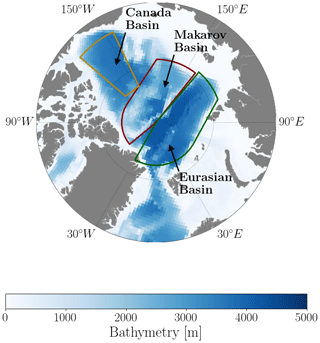
Figure 2 Bathymetry (in meters) of the ORCA1 configuration, derived from the ETOPO2 dataset. Solid colored lines show the boundaries of the Makarov (red), Eurasian (green), and Canada (yellow) basins, following Peralta-Ferriz and Woodgate (2015).

3.1 Upper-ocean properties

Figure 3 illustrates the spatial distribution of mixed-layer depth from the control run and the LOPS climatology for both March and September. Model outputs have been averaged from January 1970 to December 2021, corresponding to the same years as those observed for the MLD from the LOPS climatology. We observe that the MLD is generally underestimated by the model in September and March in the Arctic basins, especially in the areas of the Makarov and Eurasian basins next to Greenland, where the model underestimates MLD by tens of meters. Compared to a large portion of global models forced by CORE-II and JRA55-do, as studied by Ilıcak et al. (2016) and Allende et al. (2023), which include both NEMO and non-NEMO models, MLD discrepancies with observational data are less pronounced. The area along the east coast of Greenland presents pronounced MLD differences in March, with a shallower ML observed in the model than in the LOPS climatology. This region is covered with ice at that time of the year, and no MLD observations exist there, while deeper MLs are measured further offshore in the open and deep ocean. The climatology might result in an overestimation of MLD along this coast, relying solely on the data present offshore for its mapping. This would be one point to improve in a future version of this climatology. Furthermore, Fig. 4 displays the spatial distribution of sea surface temperature and salinity for the control run and the LOPS climatology. The sea surface temperature from the control run aligns with LOPS values for March and September from the three regions studied here. However, the March sea surface salinity from the control run appears to be saltier than that from the LOPS climatology for the Canada Basin and the eastern region of the Eurasian Basin, while it appears to be fresher than that from the LOPS climatology for the region next to Greenland and the western part of the Makarov Basin during September.

Figure 3 MLD maps of the control simulation, the LOPS climatology, and the differences between them for March and September. Data are averaged over the period from 1970 to 2021.

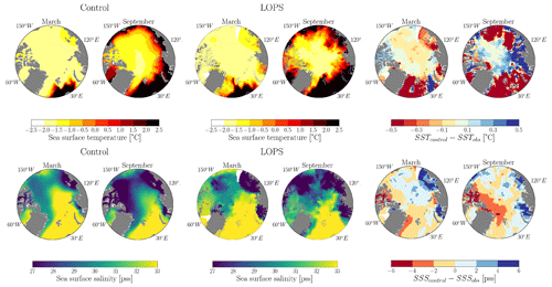
Figure 4 Sea surface temperature (SST) and sea surface salinity (SSS) maps of the control simulation, the LOPS climatology, and the differences between them for March and September with respect to the pan-Arctic region. Data are averaged over the period from 1970 to 2021. Note that “pss” stands for Practical Salinity Scale.

Figure 5 Seasonal cycle of MLD in the Makarov, Eurasian, and Canada basins. Data are averaged over the period from 1970 to 2021.

We now investigate the sensitivity of the seasonal cycle of MLD to the TKE MLP parameters previously introduced in Sect. 2. We individually modify each parameter from the control run, with each simulation named to indicate the new value of the parameter relative to the control simulation. Figure 5 illustrates the MLD seasonal cycle from the sensitivity experiments, the control run, and the LOPS climatology in each region. Data are averaged spatially and temporally for each basin. We observe similar behavior in all three regions when the TKE MLP parameters are varied. The most considerable difference between models is observed in the simulation with no attenuation in the presence of sea ice (χ=1). In such a case, significant TKE MLP mixing is induced, resulting in a deeper ML for all months compared to other simulations. When using the other three options for the scaling parameter of TKE MLP (i.e., $\mathit{\chi }=\mathrm{1}-\tanh \left(\mathrm{10}{f}_{\mathrm{i}}\right)$, $\mathit{\chi }=\mathrm{1}-f_{\mathrm{i}}$, and $\mathit{\chi }=\mathrm{1}-min(\mathrm{1},\mathrm{4}{f}_{\mathrm{i}})$), the MLD values are closer to those of the LOPS climatology. We observe that both the control run ($\mathit{\chi }=\mathrm{1}-min(\mathrm{1},\mathrm{4}{f}_{\mathrm{i}})$) and the sensitivity experiment ($\mathit{\chi }=\mathrm{1}-\tanh \left(\mathrm{10}{f}_{\mathrm{i}}\right)$) exhibit nearly identical seasonal cycles. This suggests that in these regions, the choice between attenuating mixing using a tangential hyperbolic shape or imposing a 25 % sea-ice concentration limit for mixing yields similar outcomes. When TKE penetration is turned off (f_r=0), the seasonal cycle is very weak, and the MLD is underestimated in winter. Increasing the fraction of surface TKE that penetrates into the ocean (f_r) from 0 to 0.1 increases the MLD as well as the amplitude of the seasonal cycle. As expected, a weaker-amplitude seasonal cycle is observed when varying the type of exponential decay (h_τ) from 30 to 10 m in high-latitude regions as TKE MLP vanishes more rapidly with depth.

During the summer months of July and August, all simulations underestimate the MLD compared to the LOPS climatology. These summer biases could arguably be caused by the different reference depths used for computing the MLD with the density threshold criteria: 5 m for the LOPS climatology and 0.5 m for NEMO4.2. As shown by Treguier et al. (2023), the reference depth significantly impacts the MLD. For instance, changing the reference depth in the CMCC-NEMO model from 0.5 to 10 m leads to differences in MLD exceeding 40 m across large areas of the Southern Hemisphere oceans. In the Arctic region, these differences reach a few meters. However, we recomputed the MLD using the 5 m reference for the control run and verified that such differences are not significant enough to explain the biases: the differences between the modeled MLDs computed with two reference depths were less than 5 m, and the spatial patterns between the biases of the observations and models were very similar (see Fig. A1 in the Appendix). To quantify the spatial variability in the mixed layer within each basin, we measure the MLD standard deviation for each month. The seasonal cycle of the MLD standard deviation during summer is almost negligible, and in winter, for the Makarov and Canada basins, it remains below 15 m, indicating a similar spatial variability between experiments in these regions (see Fig. A2 in the Appendix). However, for the Eurasian Basin, differences between experiments appear to be more substantial. For instance, the MLD SD reaches up to 30 m for the χ=1 experiment and is only 8 m for the f_r=0 experiment.

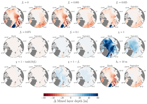
Figure 6 Maps displaying the differences in MLD between the sensitivity experiment (with the title indicating the modified parameter) and the control run for March and September. Data are averaged over the period from 1970 to 2021.

A similar pattern emerges when examining the spatial distribution of MLD. Figure 6 illustrates the differences between the sensitivity experiments and the control run for March and September. The largest ML deepening is observed when χ=1 (when there is no attenuation of mixing due to sea-ice coverage), with the MLD being at least 20 m thicker than in the control run for both months across the studied regions. Similarly, $\mathit{\chi }=\mathrm{1}-f_{\mathrm{i}}$ leads to a comparable pattern, with deeper MLs ranging from 10 to 20 m in both months. Conversely, the most significant ML shallowing is observed when f_r=0 (when TKE MLP is turned off), resulting in a ML shallower than the control by 20 m, particularly in the Canada and Eurasian basins during March. Decreasing the characteristic depth of TKE penetration (h_τ) from 30 to 10 m has an impact similar to that of a decrease in the penetrating fraction of energy (f_r), with a similar spatial distribution in both March and September. In the following, we will focus on three sensitivity experiments that differ the most from the control simulation: f_r (no TKE penetration), χ=1 (full TKE MLP below sea ice), and $\mathit{\chi }=\mathrm{1}-f_{\mathrm{i}}$ (the default sea-ice dependency of the parameterization, used in CMIP6).

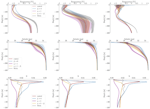
Figure 7 Vertical potential temperature in degrees Celsius, salinity in practical salinity units, and Brunt–Väisälä frequency (N) in the Makarov, Eurasian, and Canada basins (from left to right) for September. The shaded areas represent the variance. Data are averaged over the period from 1970 to 2021. The dashed lines represent the WOA climatology.

Figure 7 shows the vertical distribution of ocean physical properties, specifically stratification, salinity, and temperature, in September. To compare the stratification strength between the different simulations, we use the Brunt–Väisälä frequency, computed as

$$\begin{array}{}\text{(3)}& N=\sqrt{{\displaystyle \frac{-g}{\mathit{\rho }}}{\displaystyle \frac{\mathrm{d}\mathit{\rho }}{\mathrm{d}z}}},\end{array}$$

where g represents acceleration due to gravity approximated to 9.8 m s⁻², ρ is the potential density, and z is the vertical distance measured upward. Large values of N indicate strong stratification, and small values indicate weak stratification. We observe strong stratification in the control run and the f_r=0 experiment. On the contrary, the simulation with no attenuation of TKE MLP below sea ice is less stratified than the World Ocean Atlas (WOA) climatology. This is in agreement with the MLD: with limited vertical mixing (f_r=0), strong stratification is maintained in the upper layer, corresponding to shallow mixed layers. When TKE MLP is permitted below sea ice (χ=1), the upper ocean is less stratified and the MLD is larger. This suggests that the scaling parameter (χ), which governs TKE MLP below sea ice, significantly influences stratification. In the control run ($\mathit{\chi }=\mathrm{1}-min(\mathrm{1},\mathrm{4}{f}_{\mathrm{i}})$), TKE MLP vanishes as soon as the sea-ice concentration reaches 25 %, resulting in insufficient mixing (the stratification is too large compared to the WOA climatology). This is improved when TKE MLP varies proportionally to the sea-ice concentration ($\mathit{\chi }=\mathrm{1}-f_{\mathrm{i}}$).

Regarding the vertical temperature profiles, we observe that, compared to the control run, the f_r=0 experiment shows an increase in upper-ocean temperature, while the χ=1 and $\mathit{\chi }=\mathrm{1}-f_{\mathrm{i}}$ experiments exhibit a slight decrease. The NEMO-SI3 simulations conducted here exhibit behavior similar to that of the simulations from the first and second phases of the Ocean Model Intercomparison Project (OMIP1 and OMIP2, respectively), analyzed by Allende et al. (2023). For example, referring to Fig. 6 in the mentioned paper, we can observe that the salinity and temperature profiles of the IPSL model resemble those of the f_r=0 simulation (as expected since they deactivated the parameterization), while the CMCC profiles resemble those of the $\mathit{\chi }=\mathrm{1}-f_{\mathrm{i}}$ simulation. As studied by Ilıcak et al. (2016), the NEMO models Kiel-ORCA05, NOC, CMCC, and CERFACS underestimate the maximum temperature because Atlantic water is not well simulated in this model group (refer to Fig. 7 of Ilıcak et al., 2016). While our control simulation demonstrates improvements compared to these models, adjusting the TKE MLP parameters does not improve the representation of the temperature maximum below 200 m as this maximum is primarily affected by heat advection at this depth. The biases when using the WOA climatology for the maximum temperature correspond to approximately 0.5 °C in all three basins. The WOA climatology reaches maximum temperature values of about 0.5, 1, and 0.5 °C in the Makarov, Eurasian, and Canada basins, respectively. Similar maximum temperature values are observed using the Polar science center Hydrographic Climatology 3.0 (PHC3.0) in the Eurasian and Canada basins, as noted by Ilıcak et al. (2016). Discrepancies between experiments are also observed in the vertical salinity profiles. Compared to the control run, the simulation with no TKE penetration (the f_r=0 experiment) exhibits the freshest conditions, with a decrease in salinity of at least 2 PSU (practical salinity units) in the first tens of meters across all three basins. At the surface, salinity increases as TKE MLP intensifies; for example, in the χ=1 experiment, salinity increases by more than 2 PSU compared to the control run across all three basins. The $\mathit{\chi }=\mathrm{1}-f_{\mathrm{i}}$ experiment yields upper-ocean salinity values similar to those from the WOA climatology. In March, upper-ocean salinity differences between the experiments and the control run decrease for the χ=1 and $\mathit{\chi }=\mathrm{1}-f_{\mathrm{i}}$ simulations across the three basins. However, they remain significant for the f_r=0 simulation (see Fig. A3 in the Appendix for March profiles). Compared to the WOA climatology, all simulations except for the no-TKE-penetration simulation exhibit higher upper-ocean salinity in the Makarov and Eurasian basins. In the Canada Basin, upper-ocean salinity values are similar to those of the control run simulation.

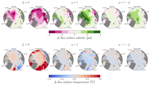
Figure 8 Sea surface salinity and potential-temperature maps of differences between the sensitivity experiments and the control simulation for March and September.

The discrepancies between the sensitivity experiments and the control run for the spatial distribution of sea surface salinity and sea surface temperature exhibit a similar pattern (see Fig. 8). A decrease in MLD with strong stratification corresponds to a reduction in sea surface salinity and an increase in surface temperature compared to the control simulation. In contrast, an increase in MLD with weak stratification is associated with an increase in sea surface salinity and a decrease in surface temperature. This can be attributed to the fact that a shallower mixed layer and strong stratification result in less mixing during ice melt, leading to a fresh anomaly at the surface and trapping heat at the surface. On the other hand, a deeper mixed layer and weak stratification allow freshwater to mix more deeply, resulting in higher surface salinity and facilitating vertical heat exchange.

3.2 Sea-ice properties

Considering the impact of the TKE MLP parameterization on the upper ocean, we expect an impact on sea-ice properties. For instance, higher sea surface salinity lowers the freezing point of seawater, delaying the formation of sea ice. Conversely, lower sea surface salinity raises the freezing point, promoting sea-ice formation. Additionally, colder sea surface temperatures encourage sea-ice formation, while warmer sea surface temperatures contribute to sea-ice melt. Figure 9 illustrates the spatial distribution of sea-ice concentration and thickness from the control run and observational data for March and September. In March, the central Arctic Ocean is almost completely covered by sea ice, with the concentration reaching nearly 100 %, and sea-ice thickness peaks between 2.5 and 3 m. By September, the effects of summer melt become evident, leading to a noticeable reduction in both sea-ice concentration and thickness. When comparing spatial patterns with observational data (OSI SAF data for sea-ice concentration and PIOMAS data for sea-ice thickness), NEMO-SI3 exhibits lower sea-ice concentration and thickness in September. Specifically, regions near the east coast (i.e., the Chukchi, East Siberian, Laptev, Kara, and Barents seas) display sea-ice thickness close to zero during this month. In March, negative biases between the simulated sea-ice thickness and PIOMAS data are more pronounced in the region next to Greenland. However, discrepancies between OSI SAF data and the simulated sea-ice concentration seem to be relatively minor.

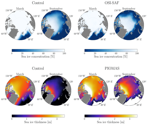
Figure 9 Maps of sea-ice concentration and sea-ice thickness for the control run and observational data concerning pan-Arctic regions with respect to the months of March and September. The data are averaged over the time period from 1970 to 2021 for the control run, and they are averaged from 1979 to 2021 for the observational data.

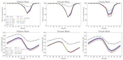
Figure 10 Seasonal cycles of sea-ice concentration and sea-ice thickness in the Makarov, Eurasian, and Canada basins. Data are averaged over the period from 1979–2021.

We analyze the seasonal cycles of sea-ice concentration and thickness in the sensitivity experiments, control run, and observational data. Figure 10 illustrates these cycles across the Makarov, Eurasian, and Canada basins, with the model variables averaged from 1979 to 2021 to align with sea-ice observational data. Compared with the OSI SAF observational data, NEMO-SI3 performs well with respect to sea-ice concentration during the winter months. However, during summer, the simulations underestimate sea-ice concentration by approximately 30 %, 48 %, and 19 % in the Makarov, Eurasian, and Canada basins, respectively, with the most significant differences occurring in August. These findings are consistent with similar observations made by Tsujino et al. (2020) for OMIP models, by Wang et al. (2016) for CORE models, and by Shen et al. (2021) for coupled models studied in CMIP5 and CMIP6 exercises in the Arctic region. Regarding sea-ice thickness, NEMO-SI3 generally simulates thinner sea ice in comparison to the PIOMAS reanalysis. Compared to the control run, the biases amount to approximately 70, 57, and 44 cm for March in the Makarov, Eurasian, and Canada basins, respectively. In September, the discrepancies reach 1.1 m across the three basins. Similar results were observed by Rosenblum et al. (2021) in the Canada Basin.

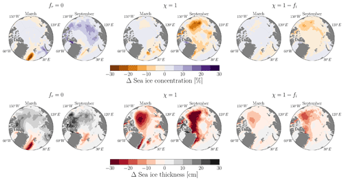
Figure 11 Maps of differences in sea-ice concentration and thickness between the sensitivity experiments and the control run for March and September. Data are averaged over the period from 1970 to 2021.

Differences between the experiments are relatively small, except in the Canada Basin during summer. The simulation with no TKE MLP (f_r=0) displays a 7 % increase in sea-ice concentration relative to the control case, while simulations with more TKE MLP below sea ice (χ=1 and $\mathit{\chi }=\mathrm{1}-f_{\mathrm{i}}$) show decreases of 10 % and 7 % in September, respectively. A similar behavior is observed for sea-ice thickness, with the largest differences between experiments observed in the Canada Basin. In September, the f_r=0 experiment shows an increase in sea-ice thickness of 14 cm, the χ=1 experiment shows a decrease in sea-ice thickness of 24 cm, and the $\mathit{\chi }=\mathrm{1}=f_{\mathrm{i}}$ experiment shows a decrease of 13 cm in sea-ice thickness relative to the control case. Figure 11 shows the differences between the sensitivity experiments corresponding to f_r=0, χ=1, and $\mathit{\chi }=\mathrm{1}=f_{\mathrm{i}}$ and the control simulation. Notably, we observe similar spatial patterns between sea-ice thickness and sea-ice concentration: an increase in sea ice for the f_r=0 simulation and a decrease for the χ=1 and $\mathit{\chi }=\mathrm{1}-f_{\mathrm{i}}$ simulations. For the χ=1 simulation, a substantial reduction in sea ice – more than ∼ 30 cm for sea-ice thickness and 20 % to 30 % for sea-ice concentration – is noticed in the area over the Beaufort Gyre. Meanwhile, for the $\mathit{\chi }=\mathrm{1}-f_{\mathrm{i}}$ simulation, the spatial differences reach more than 10 cm. These discrepancies between experiments arise from variations in the vertical profiles of density, salinity, and temperature (see Fig. 7). Strong stratification restricts vertical mixing and its associated upward vertical heat flux. This reduction in vertical heat fluxes implies less exchange between the upper ocean and sea ice, resulting in reduced sea-ice melt during the summer months, as observed in the experiment without TKE MLP (f_r=0). In contrast, weak stratification enhances vertical mixing and heat flux, leading to increased sea-ice melt, as seen in experiments with more TKE MLP below sea ice (χ=1 and $\mathit{\chi }=\mathrm{1}-f_{\mathrm{i}}$).

3.3 Interannual variability

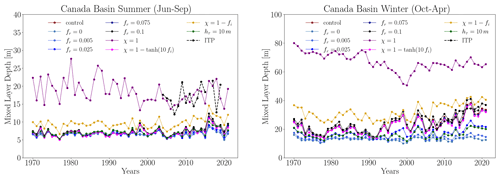
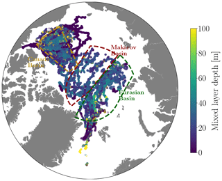
We now examine summer and winter interannual variability in the upper-ocean and sea-ice properties observed in the control run and the three sensitivity experiments – f_r=0, χ=1, and $\mathit{\chi }=\mathrm{1}=f_{\mathrm{i}}$. Figure 12 displays the evolution of MLD, sea-ice concentration, and sea-ice thickness during the summer months of June to September. Previous studies by Cole and Stadler (2019) and Wei et al. (2024), utilizing ITP observational data, highlight the increase in MLD that has occurred in the Canada Basin since 2000. We also observe this trend in MLD when examining ITP observational data for the three basins, where the linear regression slopes are 0.54, 0.37, and 0.19 m yr⁻¹ for the Makarov, Eurasian, and Canada basins. It is important to note that while this trend is well captured in the Canada Basin due to extensive ITP observations, the coverage in the Makarov and Eurasian basins is limited (see Fig. A5 in the Appendix). Although we observe an increase in MLD in these regions, further data collection is necessary to fully assess the reliability of this trend.

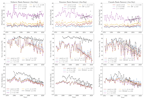
Figure 12 MLD, sea-ice thickness, and sea-ice concentration for each summer (June to September) from 1970 to 2021 in the Makarov, Eurasian, and Canada basins. Solid lines represent the linear regression, and m denotes the slope.

Consistent with Fig. 5, all experiments simulate an ML shallower than that noted in observations, except for the χ=1 experiment, which exhibits strong TKE MLP below sea ice and an excessively deep seasonal cycle. Specifically, it underestimates MLD in July and August but overestimates it in June and September. We compute the same regression for sensitivity experiments within the same time frame (from 2000 to 2021). The f_r=0 experiment (no TKE MLP) does not show an increase in MLD. All other experiments display increasing trends across the three basins, except for the χ=1 experiment, which shows a slight decrease in the Eurasian Basin ($m=-\mathrm{0.15}$ m yr⁻¹).

We also compare the summer interannual variability in the simulated sea-ice concentration and thickness with OSI SAF observational data and the PIOMAS reanalysis, respectively. Regarding sea-ice concentration, significant biases are evident in the Eurasian Basin, whereas the simulated sea-ice concentration aligns more closely with observational data from the Makarov and Canada basins. The experiments also underestimate sea-ice thickness compared to PIOMAS data from the Makarov and Eurasian basins, although the biases seem lower after the year 2000. In the Canada Basin, sea-ice thickness is close to that observed in the PIOMAS reanalysis during the full period. Focusing on the trend from 2000 to 2021, both the observational data and the model simulations show a decrease in sea-ice concentration across all three basins. In the Makarov and Eurasian basins, the decrease is stronger compared to observations; for instance, the slopes of the linear regression reach −1.18 % yr⁻¹ for the control run and −0.32 % yr⁻¹ for the OSI SAF data from the Eurasian Basin. However, in the Canada Basin, the NEMO-SI3 model captures the decreasing trend in sea-ice concentration quite well, with similar slopes for the sensitivity experiment's linear regressions compared to those from the OSI SAF. This declining trend has been previously observed and studied by Tsujino et al. (2020), Stroeve and Notz (2018), and Cavalieri and Parkinson (2012) using both observational data and model simulations. This short-term trend (from 2000 to the present) is also evident in the simulated sea-ice thickness and the sea-ice thickness from the PIOMAS reanalysis across all three basins. The loss of sea-ice thickness appears to be slower than that of sea-ice concentration, with a slope of approximately −0.04 m yr⁻¹ for the PIOMAS reanalysis across all the basins.

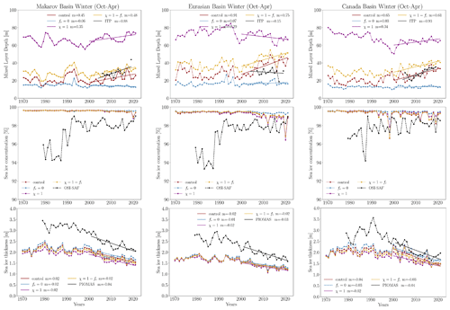
Figure 13 MLD, sea-ice thickness, and sea-ice concentration for each winter (October to April) from 1970 to 2021 in the Makarov, Eurasian, and Canada basins. Solid lines represent the linear regression, and m denotes the slope.

Figure 13 shows the winter interannual variability in MLD, sea-ice concentration, and sea-ice thickness, computed as monthly averages from October to April. As was the case in summer, the inter-model comparison reveals substantial differences in MLD. The overestimation of MLD when TKE MLP is kept below sea ice (χ=1), as shown in Fig. 5, and the underestimation when there is no TKE MLP (f_r=0) are very clear. Comparing simulations with ITP observational data, the $\mathit{\chi }=\mathrm{1}-f_{\mathrm{i}}$ and control simulations exhibit a closer resemblance. This has already been observed in the analysis of the MLD seasonal cycle. The increasing trend in MLD since 2000 is observed in ITP observational data from the Makarov and Canada basins, with values for the linear regression slope corresponding to 0.88 and 0.93 m yr⁻¹, respectively. Once again, the $\mathit{\chi }=\mathrm{1}-f_{\mathrm{i}}$ and control simulations closely resemble this behavior.

The winter interannual sea-ice concentration reaches values close to 100 %, dropping to around 98 % in some years across the Canada Basin for all simulations except the one with TKE MLP that has vanished; these values are very similar to those found in OSI SAF observational data, except those corresponding to the beginning of 1980, when sea-ice concentration decreased to 94 %. Compared with the PIOMAS reanalysis, sea-ice thickness values noted for the Makarov and Eurasian basins are larger than simulated values. Simulated sea-ice thickness ranges from 1.5 to 2 m, exhibiting a declining trend since 2000, consistent with trends observed in the PIOMAS reanalysis.

The decline in sea-ice concentration since 2000 could explain the increase in MLD for the $\mathit{\chi }=\mathrm{1}-f_{\mathrm{i}}$ and control run ($\mathit{\chi }=\mathrm{1}-min(\mathrm{1},\mathrm{4}{f}_{\mathrm{i}})$) simulations because both parameterizations involve a scaling parameter that depends on sea-ice concentration. This is not the case for the other two cases: χ=1, where TKE MLD is present everywhere, and f_r=0, where TKE MLP is not activated. Indeed, when we look at the summer and winter interannual variability in the Canada Basin for the full set of sensitivity experiments (see Fig. A4 in the Appendix), we observe that an MLD increase is present in the majority of the experiments, except the full-TKE-MLP (χ=1) experiment and those with a small percentage of surface TKE penetrating into the ocean (i.e., the f_r=0 and f_r=0.005 experiments).

4 Conclusions

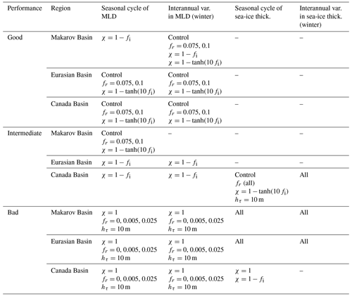
We analyzed the NEMO-SI3 model's response to changes in the TKE MLP scheme within the central Arctic Ocean, focusing specifically on the Makarov, Eurasian, and Canada basins. This parameterization is governed by three key parameters: f_r, which denotes the fraction of surface TKE that penetrates into the ocean; h_τ, representing the vertical-mixing length scale that controls the exponential shape of the penetration; and the scaling parameter (χ), applied in response to the presence of sea ice. As noted by Calvert and Siddorn (2013), Rodgers et al. (2014), and Storkey et al. (2018), the additional source of mixing provided by TKE MLP is beneficial in the NEMO model with regard to achieving realistic MLD in the Southern Ocean and in open-water regions, which we demonstrate also holds true for the Arctic region (see Table 2). Our extreme experiment (χ=1) shows that this source of mixing needs to be attenuated in the presence of sea ice. This is obvious from a physical point of view because sea ice isolates the ocean from the atmosphere and damps inertial oscillations (Rainville et al., 2011). We compared different functional forms for this attenuation. Moreover, $\mathit{\chi }=\mathrm{1}-f_{\mathrm{i}}$ is the default option in NEMO, used in most CMIP6 projections, and displays good agreement for the seasonal cycle of MLD in the Makarov Basin. However, it results in a stronger seasonal cycle of MLD compared with observations from the Eurasian and Canada basins. The two other options, $\mathit{\chi }=\mathrm{1}-\tanh \left(\mathrm{10}{f}_{\mathrm{i}}\right)$ and $\mathit{\chi }=\mathrm{1}-min(\mathrm{1},\mathrm{4}{f}_{\mathrm{i}})$, behave similarly and produce a seasonal cycle of MLD closer to that of the LOPS climatology in these regions than the 1−f_i option. Nevertheless, during summer, all experiments underestimate MLD across the three basins compared to the LOPS climatology.

Table 2 Performance summary of the TKE MLP experiments. Note that “var.” stands for variability, while “thick.” stands for thickness.

Moreover, we noticed that the choice of scaling parameter significantly affects ocean stratification and the density profile over the first 30 m of depth. We observed that changes in stratification are consistent with changes in MLD: stronger stratification corresponds to shallower MLD, while weaker stratification corresponds to deeper MLD. These changes imply significant differences in salinity near the surface. We identified an increase in salinity for simulations with an increased MLD. Conversely, simulations with a decreased MLD exhibited a decrease in sea surface salinity.

Regarding the interannual variability in MLD, we detected a short-term trend in MLD when examining ITP observational data obtained since 2000 for the three basins during summer and winter. It is important to highlight that while this trend is well captured in the Canada Basin due to extensive ITP observations, its coverage in the Makarov and Eurasian basins is limited. Although we observed an increase in MLD in all three regions, further data collection is necessary to assess whether the ML is deepening not only in the Canada Basin but also in the Makarov and Eurasian basins. The simulations with no TKE MLP do not represent the MLD trends. This raises questions regarding the choice made in some CMIP6 models to entirely remove TKE MLP, which may impact the representation of future Arctic trends.

We have investigated for the first time whether the TKE MLP scheme influences sea-ice concentration and thickness. For instance, we found a reduction in sea-ice thickness ranging from 30 to 40 cm compared to the control case when mixing was significant below sea ice (χ=1) or not completely turned off ($\mathit{\chi }=\mathrm{1}-f_{\mathrm{i}}$). Conversely, the suppression of TKE MLP created a moderate increase in sea-ice thickness, ranging from 10 to 20 cm. These discrepancies between experiments derive from variations in the vertical profiles of density, salinity, and temperature. Higher salinity in the upper layer lowers the seawater freezing point, thereby delaying sea-ice formation. Conversely, lower sea surface salinity raises the freezing point, facilitating sea-ice growth. Moreover, strong stratification restricts vertical mixing and its associated upward vertical heat flux, whereas weak stratification enhances both vertical mixing and heat flux.

This parameterization has been widely utilized in the NEMO community. Based on our study and considering the need to provide a comprehensive recommendation for NEMO users, we found that, in general, using sea-ice attenuation, either $\mathit{\chi }=\mathrm{1}-min(\mathrm{1},\mathrm{4}{f}_{\mathrm{i}})$ (control run) or $\mathit{\chi }=\mathrm{1}-\tanh \left(\mathrm{10}{f}_{\mathrm{i}}\right)$, produces more realistic MLD results and does not worsen the reproduction of sea ice. Therefore, we recommend continuing to use these parameterizations, which additionally use f_r=0.08 and h_τ=30 m. However, it is important to note that the $\mathit{\chi }=\mathrm{1}-f_{\mathrm{i}}$ simulation seemed to exhibit better agreement with sea surface salinity and temperature compared to the LOPS climatology. Moreover, the vertical properties, especially ocean stratification, appeared to be highly dependent on this attenuation parameter. A deeper understanding of this parameter is needed to improve the TKE MLP parameterization. The underestimation of sea-ice thickness and sea-ice concentration in the control run remains in all sensitivity experiments, which shows that these biases are not due to vertical mixing alone. One potential reason for this could be the ERA5 forcing, which introduces warmer temperatures into the Arctic. As shown by Batrak and Müller (2019), ERA5 exhibits a warm bias in winter, leading to thinner ice and a reduced summer extent in the model. Further investigation is needed to explore this aspect. Additionally, while this study has primarily focused on the Arctic region due to the availability of observational data for validation, it is important to evaluate how our various simulations perform in other sea-ice-covered regions.

The TKE MLP parameterization aims to reproduce the upper-ocean vertical mixing driven by near-inertial oscillations, ocean swells, and waves. However, this parameterization lacks a physical basis and is considered ad hoc (Rodgers et al., 2014). More generally, the complexity of the various TKE options has led some groups to use a generalized length-scale approach instead of the historical TKE vertical-mixing scheme (Reffray et al., 2015). Another alternative vertical-mixing scheme has been developed as part of the UK's OSMOSIS (Ocean Surface Mixing, Ocean Sub-mesoscale Interaction Study) project, which is planned to be included in the UK's Global Ocean (GO8) configuration (Storkey et al., 2018). This initiative aims to refine the characterization of near-surface oceanic mixing through a combination of observational campaigns and a novel mixing scheme derived from extensive large-eddy simulations. In particular, the Arctic region has been significantly impacted by global climate change, resulting in a rapid decrease in sea-ice extent. This phenomenon is expected to alter the exchanges between the atmosphere and ocean, thereby affecting the fully coupled ice–air–ocean system in the Arctic and consequently influencing the mechanisms driving the TKE MLP parameterization. Future research should refine our understanding of the underlying mechanisms driving the TKE MLP parameterization and explore alternative approaches to improve the robustness and accuracy of vertical-mixing parameterizations in NEMO, especially in the presence of sea ice. Such efforts will be crucial for enhancing the fidelity of Arctic climate projections and advancing our understanding of polar-climate dynamics.

Appendix A

We have compiled additional figures related to MLD maps illustrating differences in MLD based on different reference depth criteria (Fig. A1); the standard deviation of the seasonal cycle of MLD in the Makarov, Eurasian, and Canada basins (Fig. A2); vertical temperature, salinity, and Brunt–Väisälä frequency in the Makarov, Eurasian, and Canada basins during March (Fig. A3); MLD interannual variability during summer and winter in the Canada Basin (Fig. A4); and the MLD map derived from ITP data obtained over the Arctic Ocean (Fig. A5).

Figure A1 MLD maps illustrating the differences between the MLDs from the control runs computed at z_ref=5 m and z_ref=0.5 m, as well as the corresponding differences compared to the LOPS climatology, for July and August.

Figure A2 Standard deviation of the seasonal cycle of MLD in the Makarov, Eurasian, and Canada basins. Data are averaged over the period from 1970 to 2021.

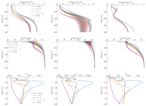
Figure A3 Vertical temperature in degrees Celsius, salinity in practical salinity units, and Brunt–Väisälä frequency (N) in the Makarov, Eurasian, and Canada basins (from left to right) for March. The shaded areas represent the variance. Data are averaged over the period from 1970 to 2021. The dashed lines represent the WOA climatology.

Figure A4 MLD interannual variability during summer (June to September) and winter (October to April) from 1970 to 2021 in the Canada Basin.

Figure A5 MLD map derived from ITP data obtained over the Arctic Ocean. Dashed lines represent the boundaries of the Makarov Basin, Eurasian Basin, and Canada Basin.