Performance and process-based evaluation of the BARPA-R Australasian regional climate model version 1

Anthropogenic climate change is changing the Earth system processes that control the characteristics of natural hazards both globally and across Australia. Model projections of hazards under future climate change are necessary for effective adaptation. This paper presents BARPA-R (the Bureau of Meteorology Atmospheric Regional Projections for Australia), a regional climate model designed to downscale climate projections over the Australasian region with the purpose of investigating future hazards. BARPA-R, a limited-area model, has a 17 km horizontal grid spacing and makes use of the Met Office Unified Model (MetUM) atmospheric model and the Joint UK Land Environment Simulator (JULES) land surface model. To establish credibility and in compliance with the Coordinated Regional Climate Downscaling Experiment (CORDEX) experiment design, the BARPA-R framework has been used to downscale ERA5 reanalysis. Here, an assessment of this evaluation experiment is provided. Performance-based evaluation results are benchmarked against ERA5, with comparable performance between the free-running BARPA-R simulations and observationally constrained reanalysis interpreted as a good result. First, an examination of BARPA-R's representation of Australia's surface air temperature, precipitation, and 10 m winds finds good performance overall, with biases including a 1 ^∘C cold bias in daily maximum temperatures, reduced diurnal temperature range, and wet biases up to 25 mm per month in inland Australia. Recent trends in daily maximum temperatures are consistent with observational products, while trends in minimum temperatures show overestimated warming and trends in precipitation show underestimated wetting in northern Australia. Precipitation and temperature teleconnections are effectively represented in BARPA-R when present in the driving boundary conditions, while 10 m winds are improved over ERA5 in six out of eight of the Australian regions considered. Secondly, the paper considers the representation of large-scale atmospheric circulation features and weather systems. While generally well represented, convection-related features such as tropical cyclones, the South Pacific Convergence Zone (SPCZ), the Northwest Cloudband, and the monsoon westerlies show more divergence from observations and internal interannual variability than mid-latitude phenomena such as the westerly jets and extratropical cyclones. Having simulated a realistic Australasian climate, the BARPA-R framework will be used to downscale two climate change scenarios from seven CMIP6 global climate models (GCMs).

1 Introduction

Australia experiences some of the highest global levels of interannual climate variability. As such, climate hazards are a key risk in Australia, encompassing wildfires (known as “bushfires” in Australia), high-intensity precipitation, tropical and extratropical storms, flooding, heatwaves, and drought. The risks associated with climate hazards are already changing as the planet warms and will continue to do so into the future. These hazards are set by a range of factors including the interaction of weather processes across the Australian geography and length scales from kilometres to hundreds of kilometres. Therefore, climate projections encompassing these scales across Australia are needed to inform the assessment of future natural hazards and associated disaster risk (Binskin et al., 2020).

Projections of hazards in Australia's climate can be sourced from dynamically downscaled climate projections: powerful tools that can help translate global climate projections to hazard-relevant length scales (Coppola et al., 2021). These projections are generated by regional climate models (RCMs), a class of climate models that focus on the simulation of a limited regional domain rather than the whole globe. Typically, RCMs are limited-area models (LAMs) with lateral boundaries sourced from global models, however complementary stretched grid models (SGMs) such as the Conformal Cubic Atmospheric Model (CCAM) can also be used for this purpose (McGregor and Dix, 2008, 2005).

RCMs have been used to study hazard projections across Australia (Herold et al., 2021) with focused studies examining changes in bushfires (Dowdy et al., 2019; Di Virgilio et al., 2019a), east coast lows and extratropical cyclones (Pepler et al., 2016; Pepler and Dowdy, 2022), heatwaves (Perkins-Kirkpatrick et al., 2016; Hirsch et al., 2019), and extreme precipitation (Bao et al., 2017), amongst others. State-based regional climate projections have been produced to assess the risks associated with a changing climate on a sub-national scale (e.g., Corney et al., 2010; Evans et al., 2014; Clarke et al., 2019; Trancoso et al., 2020).

Due to a wide range of combinations of global projections, emissions pathways, RCMs, and downscaling domains that are possible, coordination across different institutions is crucial to ensure that climate information available to users is consistent and comparable (Giorgi et al., 2009). The Coordinated Regional Climate Downscaling Experiment (CORDEX) project is an initiative of the World Climate Research Programme (WCRP) that provides a consistent framework to produce downscaled climate projections (Jones et al., 2011). Global driving model projections for CORDEX are sourced from the Coupled Model Intercomparison Project (CMIP). Due to computational expense, the full CMIP ensemble generally cannot be downscaled, and a representative subsample may be coordinated instead at a regional level (e.g., Grose et al., 2023). CORDEX has defined a set of 16 climate regions, including the Australasian region, which consists of Australia, New Zealand, the western Pacific, and parts of Southeast Asia (shown in red in Fig. 1). Six dynamical RCMs, produced using five independent modelling frameworks, contributed downscaled projections of the Australasian region to the first Coordinated Regional Climate Downscaling Experiment (CORDEX-CMIP5) (Di Virgilio et al., 2019a; Evans et al., 2021).

When downscaling ERA-Interim reanalyses, the CORDEX-Australasia CMIP5 ensemble framework featured persistent cold daily maximum biases on the order of 2–5 ^∘C, reduced diurnal temperature ranges, and dual-signed precipitation biases with magnitudes of up to 40 mm per month (Di Virgilio et al., 2019b). Downscaling of the CMIP5 historical experiment model ensemble reflected these temperature biases and showed dry precipitation biases in the tropical monsoonal regions and wet biases elsewhere (Evans et al., 2021). However, Evans et al. (2020) showed that the CORDEX-CMIP5 Australasia ensemble generally outperformed the driving global climate model (GCM) ensemble, particularly at simulating the tails of temperature and precipitation distributions.

Here, we introduce the Bureau of Meteorology Atmospheric Regional Projections for Australia (BARPA-R), an RCM designed for the Australasian region. BARPA-R is being developed by the Australian Bureau of Meteorology (henceforth the Bureau) and the Australian Climate Service (ACS), together with a forthcoming convection permitting model, BARPA-C. The BARPA-R model configuration and developmental trials were presented by Su et al. (2022b). This model is a continuation of prototype work developed for the Energy Sector Climate Information (ESCI) project, documented by Su et al. (2021) and from hereon referred to as ESCI-BARPA. BARPA-R adheres to the principle of seamless weather and climate prediction by following the Australian Community Climate and Earth-System Simulator (ACCESS) modelling framework and uses a 17 km (0.1545^∘) grid spacing. This means that BARPA-R uses an atmospheric model configuration that is complementary to the Bureau's operational numerical weather prediction (NWP) configuration and seasonal prediction configuration, allowing learning and development from NWP to be applied over longer timescales into the regional climate change space. Furthermore, BARPA-R is being developed in tandem with BARRA2 reanalysis (version 2 of the Bureau of Meteorology high-resolution Atmospheric Regional Reanalysis for Australia, Su et al., 2022a), allowing for seamless comparison between the data-assimilated and fully model-based simulations.

The Bureau intends to downscale an ensemble of at least seven CMIP6 global climate models (GCMs) using the BARPA-R framework. Downscaling GCMs have been selected based on their performance over Australia, representation of climate drivers, modelling centre independence, and the overall ensemble coverage of a range of warming and precipitation change scenarios in the Australian region, following Grose et al. (2023). Through ACS, BARPA-R is intended to produce complementary regional climate projections to existing Australian RCM systems, broadening the ensemble of climate hazard projections available in the Australasian region. BARPA-R will be compliant with next generation of CORDEX, CORDEX-CMIP6. Since the atmospheric component of ACCESS and the UK Met Office's Unified Model (MetUM) are co-developed and share a code base, BARPA-R also joins a family of MetUM-based regional climate simulations around the world. These include the PRECIS regional climate modelling system, CP4Africa (Stratton et al., 2018), and the HadREM CORDEX-Europe (Tucker et al., 2022) simulations.

This paper presents an assessment of the BARPA-R evaluation simulation. The evaluation simulation is driven at the lateral boundaries using ERA5 reanalysis (Hersbach et al., 2020) and is designed to test the performance of the RCM. This paper proceeds as follows. In Sect. 2, descriptions of the BARPA-R model configuration, the evaluation methodology, and the reference datasets are provided. Section 3 evaluates the performance of BARPA-R in simulating the observed precipitation and temperature and near-surface wind climates in the Australian region. Section 4 provides a process-based evaluation in order to assess the representation of key circulation features and weather systems in the Australian region.

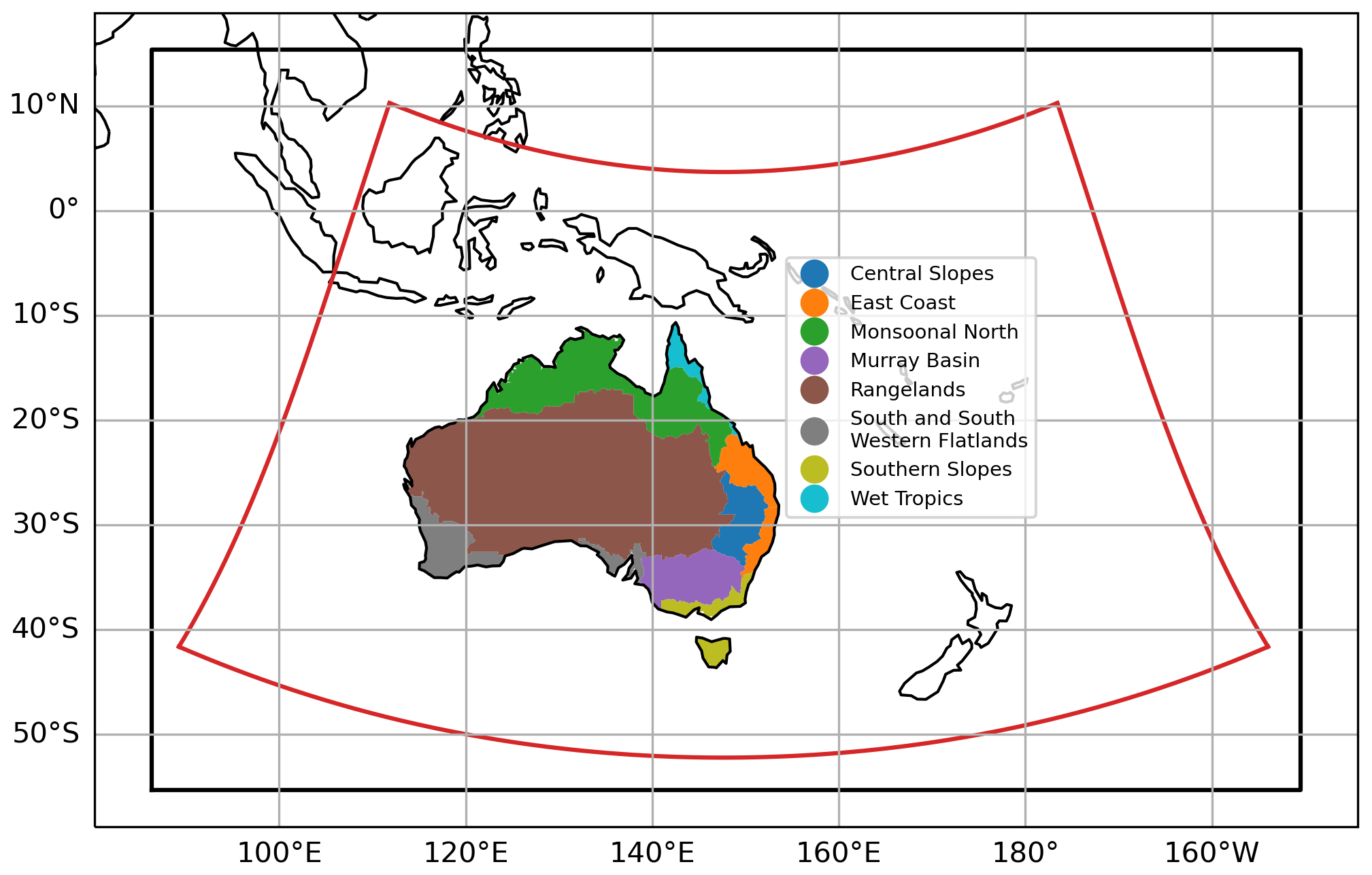
Figure 1 Map of the region of interest with the BARPA-R domain marked by a black box and CORDEX-Australasia domain marked by a red box. The National Resource Management (NRM) clusters described in Sect. 2.3 and used in model evaluation are indicated in colours as per the figure legend.

2 Data and methods

2.1 Experimental design and model configuration

BARPA-R is a land–atmosphere limited-area regional climate model. The experimental design follows the CORDEX-v2 Australasia guidelines. The limited-area domain covers the CORDEX-Australasia domain, as shown in Fig. 1, and includes Australia, New Zealand, the western Pacific, and the Maritime Continent. The horizontal grid spacing is 0.1545^∘ in latitude and longitude, which roughly corresponds to 17 km in each direction. A total of 63 vertical model levels have been used, with a 40 km model top. A stretch sigma grid is used with a higher density of levels near the surface, with the first model level is located 10 m above ground level (a.g.l.). Model levels are terrain following near the surface and relax to surfaces of uniform radial height approximately 18 km a.g.l. The model integration updates on a 7.5 min dynamical time step.

The simulation was initialised from the deterministic ERA5 reanalysis on 1 January 1979. Soil moisture was initialised from the 1 January climatological mean of the BARRA-V1 reanalysis (Su et al., 2019). Boundary conditions were updated every 3 h and derived from the ERA5 pressure level dataset, which consists of 37 vertical levels. The 3D model inputs from ERA5 at the lateral boundaries were horizontal winds, specific humidity, temperature, cloud liquid, cloud ice, and cloud cover. Between 2000 and 2006, boundary inputs were derived from ERA5.1 to avoid stratospheric temperature and humidity biases present in the original ERA5 dataset. Sea surface temperatures were sourced from ERA5 and updated daily. Model configuration followed the MetUM standard configuration HadREM3-GA7.05 (Tucker et al., 2022) with a few modifications as described in the BARPA-R version 1 model description paper (Su et al., 2022b). Firstly, the “fountain buster” correction to the advection scheme was applied to improve moisture conservation during strong convective events. Secondly, the “prognostic entrainment” scheme (Willet and Whitall, 2017) was applied to improve the representation of convection and precipitation. Thirdly, Newtonian relaxation (Telford et al., 2008; Stassen et al., 2023) is used to improve alignment between the driving model and the interior of the domain. This relaxation is applied from model level 38 and above (11 km a.g.l.) with a 6 h relaxation timescale. These modifications were demonstrated in trial experiments to improve the climatologies of Australian precipitation and near-surface temperatures. The University of Melbourne (UM) and Joint UK Land Environment Simulator (JULES) code branches used in the publication have not all been submitted for code review and inclusion in the UM/JULES trunk or released for general use. These branches are associated with nudging, support for the 365 d calendars used by some GCMs, and performance optimisation for the Australian national computational infrastructure (NCI) and were provided to the reviewers of this article.

HadREM3-GA7.05 uses a non-hydrostatic, fully compressible, deep atmosphere formulation with an iterative, semi-implicit dynamical solver (Wood et al., 2014). Awakara-C grid staggering is used in the horizontal dimensions (Arakawa and Lamb, 1977), and Charney–Phillips staggering is used in the vertical dimensions. Key parameterisation schemes include the prognostic condensate (PC2) cloud scheme (Wilson et al., 2008), the Lock et al. (2000) boundary layer scheme, the Gregory and Rowntree (1990) mass flux convection scheme, the Edwards and Slingo (1996) radiation scheme and the Wilson and Ballard (1999) mixed-phase cloud microphysics. These schemes have been routinely improved since their publication through regular model development (Walters et al., 2019). Observed historical greenhouse gas, aerosol, and ozone forcing are implemented following Tucker et al. (2022). This approach prescribes 4D aerosol optical properties on nine shortwave and six longwave bands in the SOCRATES radiative transfer code, combining seasonal and spatial variation derived from an offline simulation using the Global Model of Aerosol Processes (GLOMAP) scheme (Mann et al., 2010) with interannual variation derived from the EasyAerosol project (Stevens et al., 2017).

The MetUM atmosphere is coupled to the Joint UK Land Environment simulator (JULES, Best et al., 2011). JULES uses a nine-tile approach to represent sub-grid-scale land cover heterogeneity, namely broadleaf and needle-leaf trees, C₃ and C₄ grass, shrubs, inland water, bare soil, urban areas, and land ice. Four soil levels are present with thicknesses of 0.1, 0.25, 0.65, and 2 m. In BARPA-R, land surface properties are prescribed as per Walters et al. (2019), with the exception of the land sea mask, which is derived from the ERA Climate Change Initiative (CCI, Hartley et al., 2017), and the broadleaf canopy height, which is derived from Simard et al. (2011) following Dharssi et al. (2015). Land cover categorisation is fixed using a seasonal climatology following Hurtt et al. (2020).

2.2 Reference datasets

This paper evaluates the performance of BARPA-R against three main observationally derived datasets: version 1 of the Australian Gridded Climate Dataset (AGCD, also known as AWAP), the ERA5 deterministic reanalysis, and the Australian Bureau of Meteorology's point-based station dataset. The current BARRA-V1 regional reanalysis is not used in this work as our core evaluation period goes back to 1985.

AGCD is a near-surface analysis product that uses an anomaly-based modified Barnes successive corrective method to interpolate gridded station data to a regular grid (Jones et al., 2009). In this work, AGCD version 1 is used to evaluate the ability of the BARPA-R system to reproduce the observed temperature and precipitation climate across Australian land points. The three AGCD variables used in this study, daily maximum temperature, daily minimum temperature, and daily total precipitation, are available on a regular grid with 0.05^∘ latitude and longitude spacing. AGCD's performance hinges on the availability of station data, and it thus suffers from data availability issues in sparsely populated regions. A spatial mask, shown in Fig. 2, is applied to precipitation metrics to remove the influence of regions most poorly constrained by observations; however, observational uncertainty in the AGCD dataset remains.

Jones et al. (2009) describe key sources of observational uncertainty in AGCD. They highlight underestimations of maximum temperatures in regions of tight climate gradients and sparse observational coverage, including coastal northwestern Australia and the Nullarbor Plain, due to the poor resolution of maritime effects. They also note large analysis errors in daily precipitation estimates, with mean absolute errors up to 50 % of the total. King et al. (2013) demonstrated that AGCD is suitable for the study of rainfall extremes, trends and variability across much of Australia, with limitations occurring in regions where station coverage is sparse. Meanwhile, Chubb et al. (2016) established large systematic dry biases between AGCD and an independent gauge network in the Snowy Mountains. In the following analysis, the direction of the AGCD biases is opposite to the BARPA-R bias presented. This means that the biases presented in this paper are likely overestimates, ensuring that our analysis is conservative.

ERA5 (Hersbach et al., 2020) is a global reanalysis product that combines data assimilation with ECMWF's Integrated Forecasting System (IFS) model. As well as providing boundary conditions, ERA5 is used in the assessment of the BARPA-R evaluation simulation. In the performance evaluation section below, BARPA's biases are compared to ERA5's biases, both with respect to AGCD. However, since ERA5 benefits from assimilating observations while BARPA-R is a free running model within its regional boundaries, this reference is not regarded to be a minimum benchmark for some metrics. For example, it is not expected that BARPA-R will outperform ERA5 based on direct comparisons with observations at exact times and locations. When comparable levels of performance are present in BARPA-R and ERA5, this is interpreted as a good result for BARPA-R. There are also expectations that some climatological metrics could indicate benefits from the BARPA-R downscaling, such as metrics based on spatio-temporal averages of weather conditions.

2.3 Evaluation methodology

In Sect. 3, the temperature and precipitation climatology is evaluated through analysis of derived standardised climate indices defined in the ICCLIM project (Pagé et al., 2022). These indices have been selected to evaluate aspects of the tails of the precipitation and temperature distributions, such as monthly maximum and minimum temperatures and high precipitation rates. Indices have been computed on the 0.25^∘ ERA5 grid following conservative remapping, aggregating from daily temperature extrema and precipitation data to monthly indices.

Performance was assessed over eight Australian regions, known as the National Resource Management (NRM) clusters (Clarke et al., 2015). These clusters are shown in Fig. 1 and have been designed to be climatologically distinct and follow the boundaries of the Australia's 54 National Resource Management regions. This assessment is based on the decomposition of root-mean-square error into bias, correlation, and variance error metric components following Su et al. (2013) and Gupta et al. (2009) and presented in Eq. (1). Error metrics selected were the seasonal biases, annual variance errors, climatological seasonal correlations, and climatological spatial correlations. These error metrics are adjusted to reflect important climatological aspects of model performance, as a like-for-like reproduction of observed weather events is not expected from free-running climate downscaling experiments.

$$\begin{array}{}\text{(1)}& {\displaystyle }\begin{array}{rl}{\text{RMSE}}^{\mathrm{2}}& =\underset{\text{corr}}{\underbrace{\text{correl}(m,o{)}^{\mathrm{2}}}}-\underset{\text{var error}}{\underbrace{{\left(\text{correl}(m,o)-{\displaystyle \frac{\text{SD}\left(m\right)}{\text{SD}\left(o\right)}}\right)}^{\mathrm{2}}}}\\ & -\underset{\text{bias}}{\underbrace{{\left({\displaystyle \frac{\frac{\mathrm{1}}{n}\sum m-\frac{\mathrm{1}}{n}\sum o}{\text{SD}\left(o\right)}}\right)}^{\mathrm{2}}}}\end{array}\text{(2)}& {\displaystyle }{\text{bias}}_{\text{DJF}}={\displaystyle \frac{\mathrm{1}}{n}}\sum _{x,y}\left({\displaystyle \frac{\mathrm{1}}{\mathrm{90}}}\sum _{t\in \text{DJF}}m-{\displaystyle \frac{\mathrm{1}}{\mathrm{90}}}\sum _{t\in \text{DJF}}o\right)\text{(3)}& {\displaystyle }{\text{bias}}_{\text{JJA}}={\displaystyle \frac{\mathrm{1}}{n}}\sum _{x,y}\left({\displaystyle \frac{\mathrm{1}}{\mathrm{90}}}\sum _{t\in \text{JJA}}m-{\displaystyle \frac{\mathrm{1}}{\mathrm{90}}}\sum _{t\in \text{JJA}}o\right)\text{(4)}& {\displaystyle }\text{var error}={\displaystyle \frac{\mathrm{1}}{n}}\sum _{x,y}{\displaystyle \frac{{\text{SD}}_{\mathrm{year}}\left({\mathrm{\Sigma }}_{\mathrm{mon}}\frac{m}{\mathrm{12}}\right)+\mathrm{1}}{{\text{SD}}_{\mathrm{year}}\left({\mathrm{\Sigma }}_{\mathrm{mon}}\frac{o}{\mathrm{12}}\right)+\mathrm{1}}}-\mathrm{1}\text{(5)}& {\displaystyle }{\text{corr}}_{\text{seas}}={\displaystyle \frac{\mathrm{1}}{n}}\sum _{x,y}{\text{correl}}_{\mathrm{mon}}\left({\displaystyle \frac{\mathrm{1}}{\mathrm{30}}}\sum _{\mathrm{year}}m,{\displaystyle \frac{\mathrm{1}}{\mathrm{30}}}\sum _{\mathrm{year}}o,\right)\text{(6)}& {\displaystyle }{\text{corr}}_{\text{spatial}}={\text{correl}}_{x,y}\left({\displaystyle \frac{\mathrm{1}}{\mathrm{360}}}\sum _{\mathrm{time}}m,{\displaystyle \frac{\mathrm{1}}{\mathrm{360}}}\sum _{\mathrm{time}}o,\right)\end{array}$$

Here, m and o represent the three-dimensional, monthly modelled and observed indices, respectively; SD_x and correl_x represent the act of computing the standard deviation or Pearson correlation of inputs over dimension x; and n indicates the number of grid points in the NRM cluster of consideration. The variance formula is modified by an offset of 1 to avoid division by zero in regions of low rainfall.

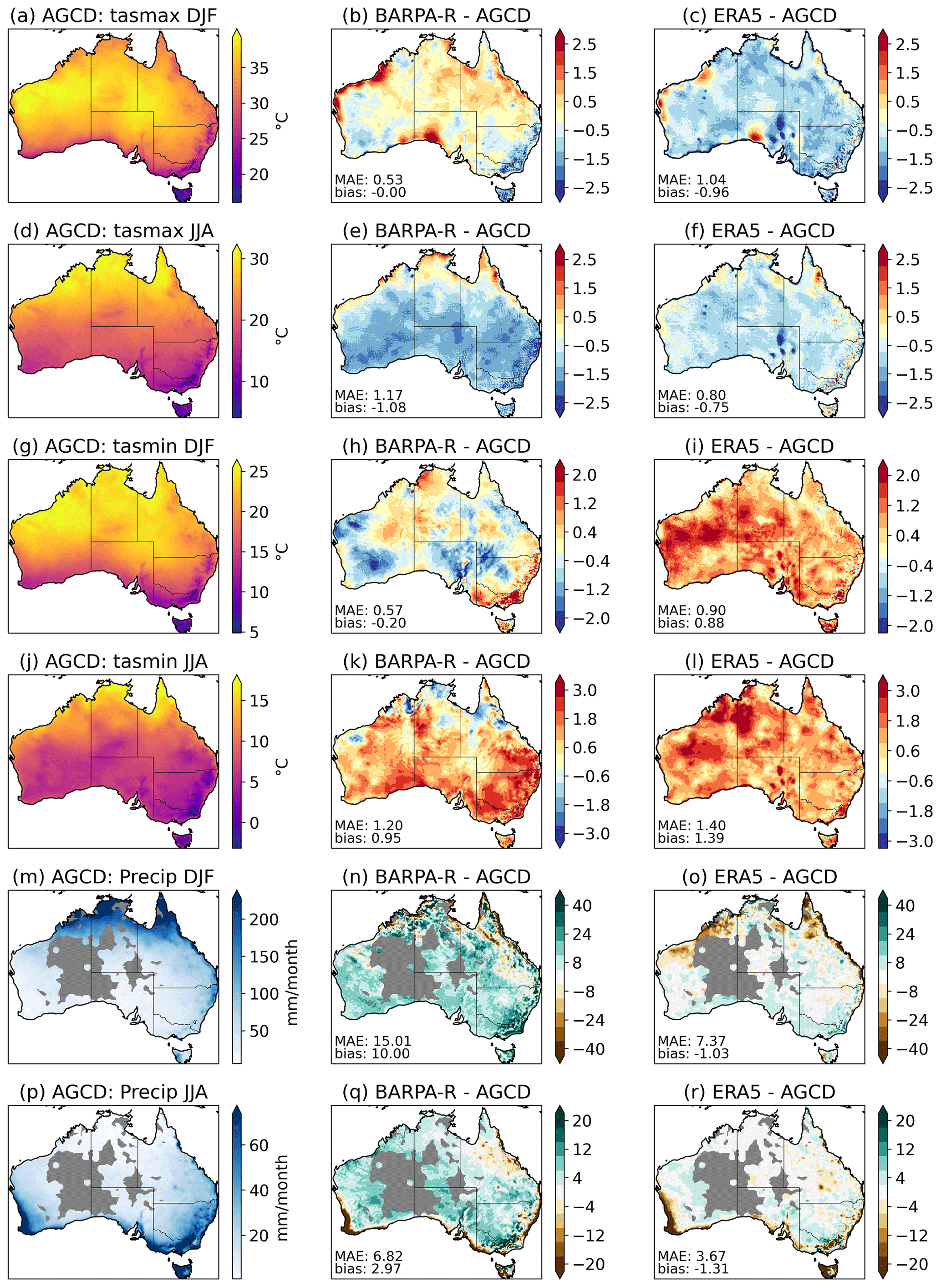
Figure 2 Bias in temperature and precipitation climate indicators (rows: TX, TN, and PRCPTOT) for two seasons, DJF and JJA, for BARPA-R and ERA5 (second and third columns) against AGCD (first column) averaged across the core evaluation period (1985–2014). The annotated figures indicate the area-averaged bias (top) and mean absolute error (bottom).

3 Performance evaluation

3.1 Mean state

This section evaluates the performance of BARPA-R at simulating Australian monthly temperature and precipitation metrics as compared to AGCD and ERA5. Firstly, we examine the mean state bias maps of seasonal-mean daily maximum and minimum temperatures and precipitation. Secondly, spatial and temporal characteristics of six temperature and four precipitation indices are examined, aggregated over the eight NRM clusters. These indices were chosen with some emphasis on including properties of high-impact weather. Finally, contemporary climate trends of the same 10 indices are compared across the three data products.

Figure 2 displays seasonal bias maps over the Australian region of daily minimum temperature, daily maximum temperature and monthly precipitation totals, all averaged over the core evaluation period (1985–2014). Two seasons are presented here: December to February (DJF) and June to August (JJA). The remaining transition seasons are provided in Fig. A1. When temperature biases show a decrease in maximum temperatures coupled to an increase in minimum temperatures in the same season, this can be interpreted as an underestimation of the diurnal temperature range. During the Austral summer and northern Australian wet season, BARPA-R shows improvements in both daily minimum and daily maximum temperatures compared to ERA5, whose diurnal temperature range is reduced compared to observations across the country. However, BARPA-R does show a reduced diurnal temperature range across the southeastern coast. Persistent warm biases of daily maximum temperatures in the Nullarbor may derive from observational uncertainty due to the low density of station data contributing to AGCD in these regions (Jones et al., 2009).

During the winter season, both BARPA-R and ERA5 show a reduced diurnal temperature range compared to the observed climate, with overly warm minimums and cool maximums, except for in the tropical north. The magnitude of the biases is higher in BARPA-R than ERA5, particularly on the highly populated Australian East Coast. In all seasons, BARPA-R has a more realistic representation of Australia's inland lakes than ERA5.

The final two rows of Fig. 2 show the monthly aggregated precipitation biases. Overall, BARPA-R is overly wet, consistent with the overall performance of ACCESS-based models in the Australian region, including in NWP (Hudson et al., 2017). A prominent wet bias is present over the highlands in eastern Victoria in both seasons. However, wet biases surrounding the two masked regions in Western Australia (grey) are likely to be related to underestimates in AGCD due to the sparse station network (Jones et al., 2009). BARPA-R shows a reduction in ERA5's dry biases in southwestern Australia, western Tasmania, the Pilbara, and Cape York.

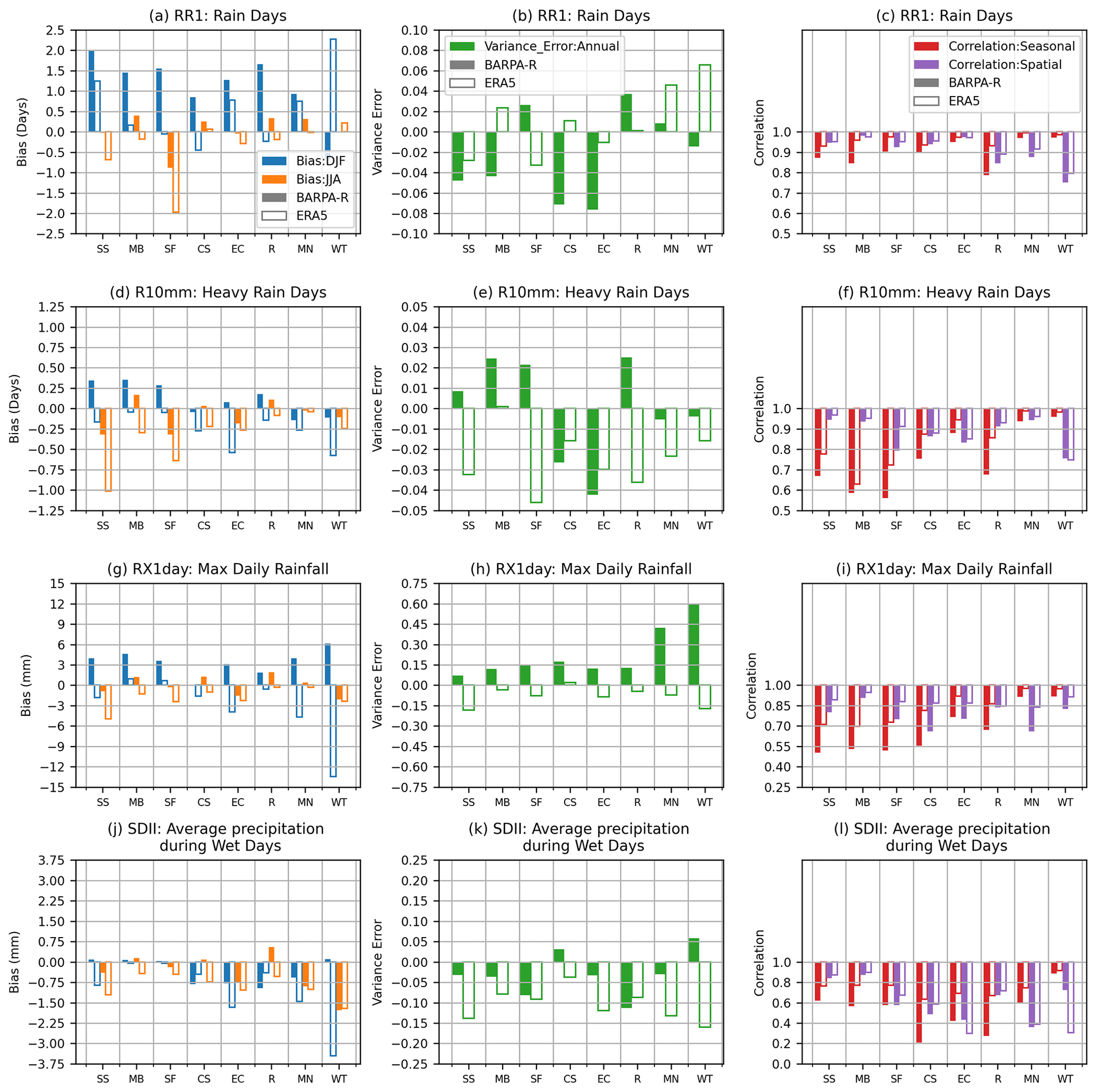
Figure 3 BARPA-R (solid bars) and ERA5 (outlined bars) performance of six temperature indices across the eight Australian NRM clusters. Reference data are sourced from AGCD. Rows show number of summer days (SU; with daily maximum temperatures exceeding 25 ^∘C), tropical nights (TN; with daily minimum temperatures exceeding 20 ^∘C), and the monthly minimums and maximums of the daily minimums and maximums (TNn, TNx, TXn, and TXx). Skill metrics are indicated by colour and column, with blue and orange showing the bias aggregated over summer and winter, respectively (left), green representing the ratio of interannual standard deviations (middle), red representing the correlations in the climatological seasonal cycles, and purple representing the spatial correlation across the NRM cluster of the climatological mean (right). All temporal metrics are computed at each grid point and then spatially aggregated.

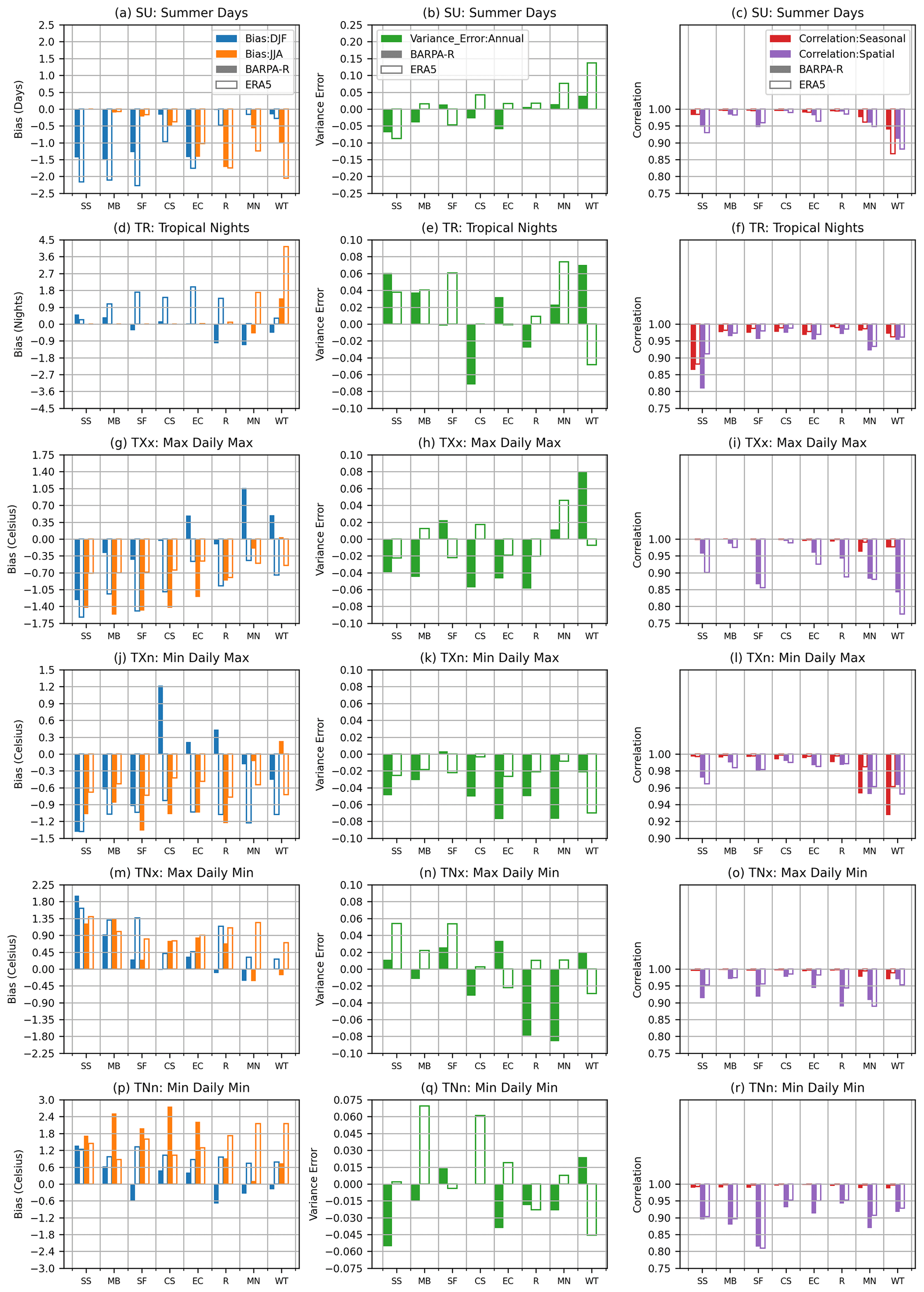
Figure 4 As per Fig. 3 but for precipitation indices: wet days (RR1, >1 mm d⁻¹), heavy rain days (R10mm; >10 mm d⁻¹), monthly maximum daily precipitation (RX1day), and monthly precipitation (PRCPTOT).

Six temperature indices have been selected to examine BARPA-R's representation of Australia's regional temperature climates. The indices considered are the number of summer days (SU; T_max>25), number of tropical nights (TN; T_min>20), the monthly minimums and maximums of the daily minimums (TNn, TNx), and the same of the daily maximums (TXn, TXx). These indices have been computed on a monthly timescale from daily maximum and minimum temperature data for AGCD and ERA5 and then regridded to the BARPA-R grid as described in Sect. 2. Performance statistics described in Sect. 2.3, namely biases, variance errors, and correlations of the seasonal cycles, are calculated at each grid point and then averaged across each NRM cluster. A spatial correlation was additionally calculated on the overall climatological mean of each index for each NRM cluster.

The resultant statistics are presented in Fig. 3. The number of summer days is substantially improved in BARPA-R compared to ERA5, with reduced biases in most cases (save for summer in the north-most clusters), similar spatial correlations, and a much-improved seasonal cycle in the wet tropics. Tropical nights also show reduced biases but worse variance errors in many cases and worse performance in the South Slopes cluster. Absolute monthly maximum temperatures exhibit a strong cold bias in BARPA-R throughout the southern NRM clusters, consistent with the results shown in Fig. 2.

The equivalent bar charts for precipitation-based variables are shown in Fig. 4. The metrics selected were number of rain days (RR1, with at least 1 mm of daily precipitation; heavy precipitation days (R10m, with at least 10 mm of daily precipitation); the monthly maximum daily precipitation amount (Rx1day); and the Simple Daily (precipitation) Intensity Index (SDII), which is calculated as the average precipitation rate across all days with at least 1 mm of precipitation. BARPA-R's wet bias is generally visible across the first three of these metrics, with BARPA-R biases generally tending towards more precipitation and rain days and being larger in magnitude than the ERA5 biases. Exceptions to this include the winter rain and heavy rain day count in the southern and southwestern flatlands, which are negative and reduced compared to ERA5, and rain days in the two tropical clusters where large positive biases in ERA5 are improved by BARPA-R. Maximum daily precipitation is consistently more variable on an interannual timescale in BARPA-R than in AGCD across all NRM clusters. However, the SDII has a consistent negative bias across ERA5 that is significantly improved in BARPA-R, particularly during the summer months. Both SDII and maximum daily precipitation have low spatial and seasonal correlation values, consistent with expectation that these fields will be quite noisy due to the influences of extreme values.

3.2 Trends

In order for the BARPA-R system to be of use in dynamically downscaling climate projections, it is crucial that BARPA-R is able to sensibly simulate changes in climate. Additionally, the subset of CMIP6 that will be downscaled with BARPA-R has been selected to cover a range of wetting and drying and high and low warming scenarios, with the intention that BARPA-R outputs can be used in a larger ensemble together with projections from other RCMs within CORDEX Australasia. Although it is possible that BARPA-R may be found to diverge from its host GCM for good reasons, this model selection was based on the hypothesis that this spread in future change will be translated to some degree into the BARPA-R ensemble. Therefore, this section investigates the degree to which BARPA-R is able to simulate observed trends in contemporary climate.

The study periods used for this analysis are two 10-year time slices: 1985–1994 and 2005–2014. Due to their short durations, these time slices will include a degree of interannual variability as well as any anthropogenic climate change. However, it is expected that this variability will be in phase and consistent across the observations and driving reanalysis data, and therefore should be reproducible by BARPA-R.

This trend analysis must be caveated by the observational uncertainties associated with the trends of both AGCD and ERA5. Long-term trends in observational datasets, including analyses and reanalyses, are sensitive to temporal inhomogeneities in their input datasets (Gibson et al., 2019, e.g.,). Simmons et al. (2021) found that temperature trends over Australia are affected by inhomogeneities in the observational inputs; however, the poorest performance occurs prior to 1970, before our study period. AGCD has been designed to be more robust to long-term trends through the application of an anomaly-based approach that takes advantage of climate normals at a subset of stations with longer coverage. Jones et al. (2009) demonstrate that this approach provides consistent maps of precipitation trends compared to monthly analyses derived only from stations with long climate records and found that temperature trends were similarly robust at the large scale.

With these caveats in mind, this paper accounts for observational uncertainty in rainfall trends by focussing attention on established trends that have been studied elsewhere, namely southern Australian cool-season drying, wetting trends in northwestern Australia during summer, and the intensification of short-duration heavy convective rainfall (Tolhurst et al., 2023; Borowiak et al., 2023; Fowler et al., 2021).

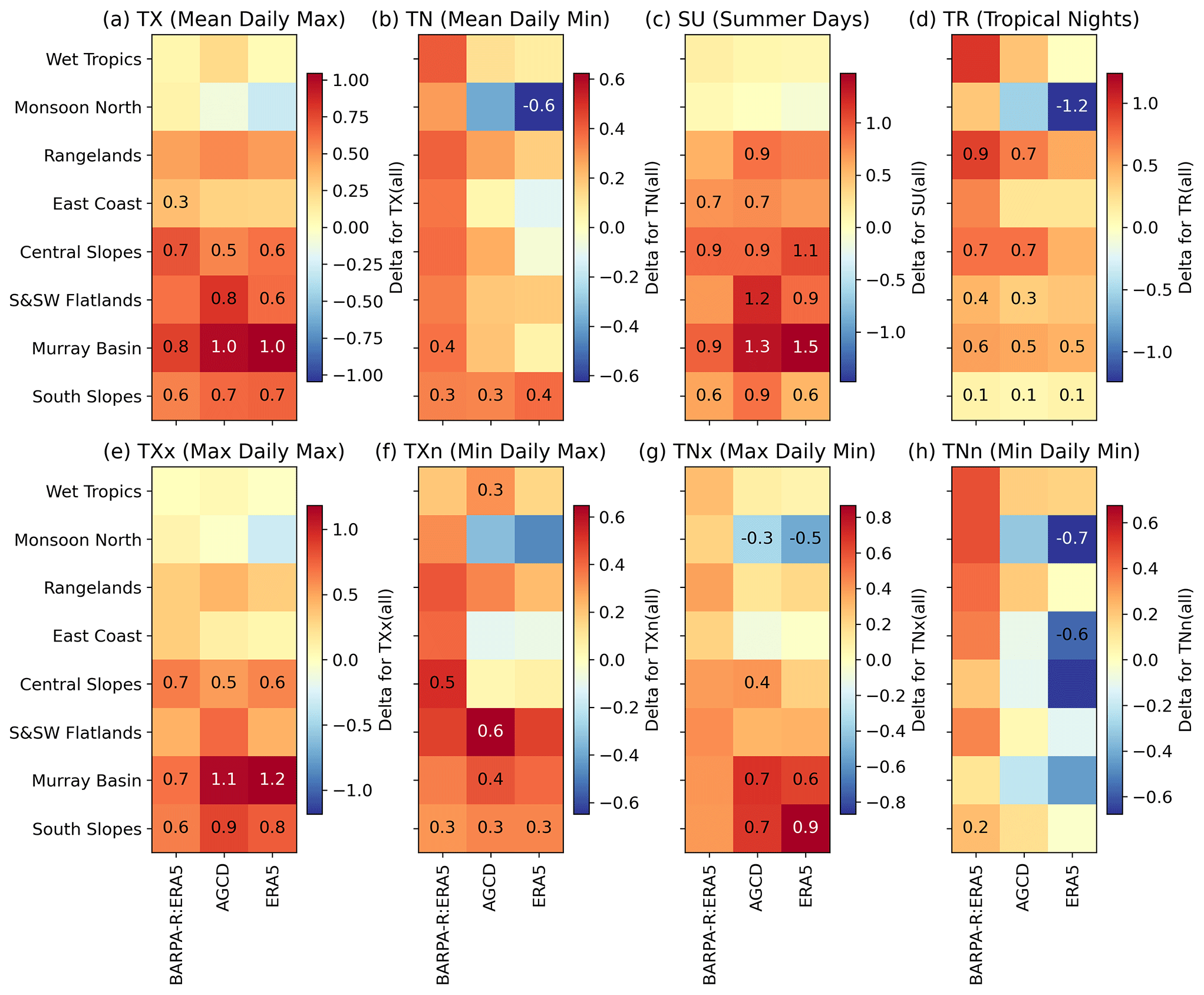
Figure 5 Contemporary change in annual means of eight temperature indices between the period 1985–1994 and 2005–2014 aggregated across NRM clusters. Indices are as per Fig. 3, together with the monthly mean daily temperatures (TX and TN). Values are annotated on the panels when the early and late samples are significantly distinct at the p>0.05 level using a Welch's t test.

The contemporary change in the temperature-based ICCLIM indices across BARPA-R, AGCD, and ERA5 are shown in Fig. 5. BARPA-R shows warming trends for all the indicators across all the clusters. There is some consistency between BARPA-R and AGCD, particularly for the indicators based on maximum temperatures. Statistically significant AGCD trends present in monthly mean maximum temperature (TX), summer days (SU), and monthly maximum temperature (TXx) in the southern clusters are generally well captured and significant in both BARPA-R and AGCD. However, minimum temperature-based indices show increased rates of warming in BARPA-R that are not reflected in the observed products. Aside from in the Murray basin cluster, these changes are not statistically significant at the p<0.05 level. However, some cooling trends are observed in AGCD and ERA5 that are not present in BARPA-R, most noticeably in the monsoonal north and in absolute minimum temperatures.

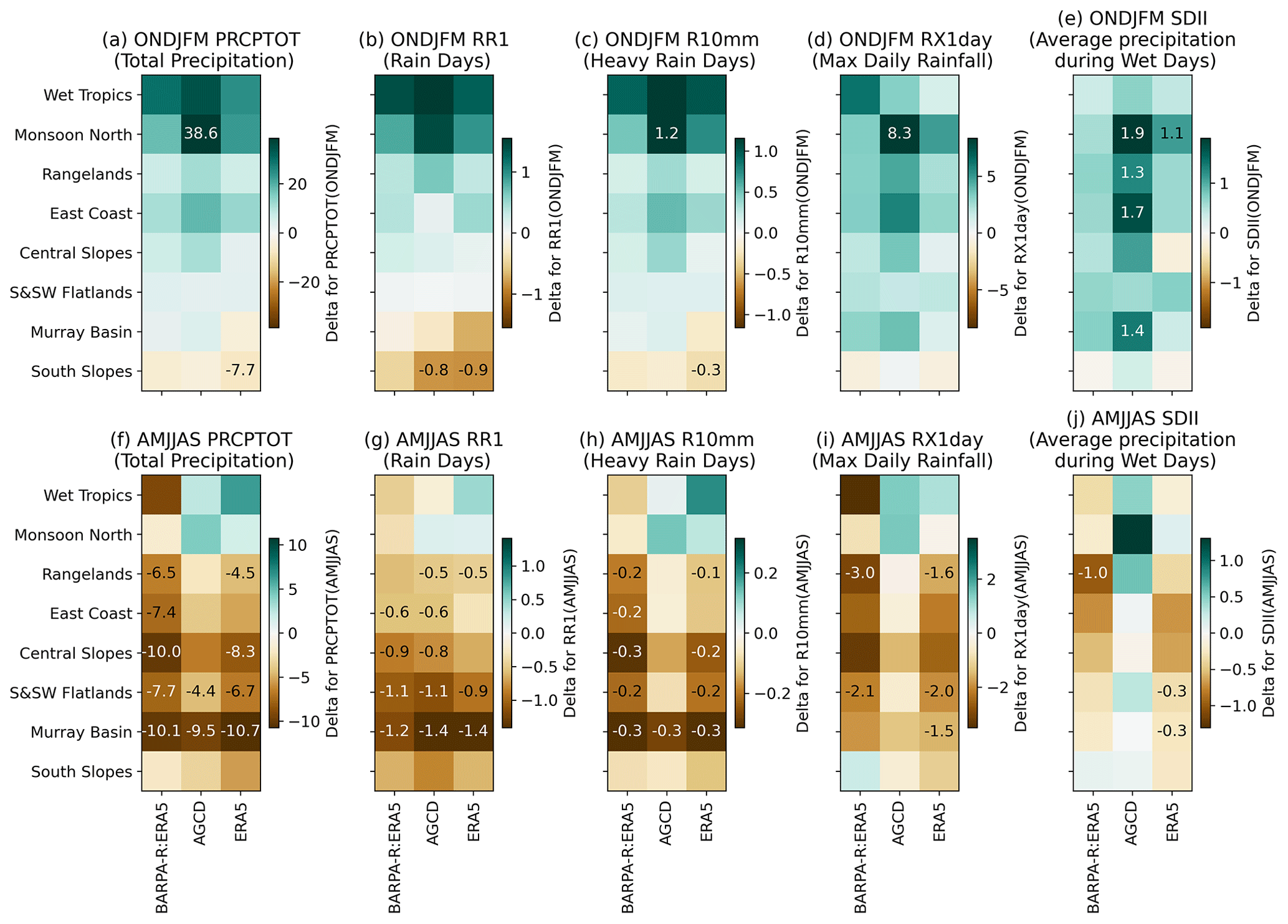
Figure 6 Contemporary change in seasonal means of five precipitation indices between 1985–1995 and 2005–2015. Indices are as per Fig. 4, together with monthly total precipitation (PRCPTOT). Values are annotated on the panels when the early and late samples are significantly distinct at the p>0.05 level using a Welch's t test.

Corresponding trend plots for precipitation indices are shown in Fig. 6. As contemporary trends show a strong seasonal dependence, these trends have been split into warm-season (October–March) and cool-season (April–October) panels. The direction of change is generally consistent across all three datasets in the warm season. Significant AGCD-based increases in precipitation intensities across multiple NRM clusters (Fig. 6e) are not reflected in either BARPA-R or ERA5. This result highlights the difficulty that parameterised convection models and reanalysis products have in simulating the observed intensification of short-duration extreme precipitation (Fowler et al., 2021). A decrease in the number of dry days in the southern slopes region is evident in ERA5 but insignificant in BARPA-R. Conversely, in the cool-season drying trends are typically more pronounced in BARPA-R and ERA5 than in AGCD. Reductions in rain days are consistent across all three datasets.

3.3 Interannual variability

BARPA-R outputs are examined here in relation to three key modes of interannual climate variability: the El Niño–Southern Oscillation (ENSO), the Indian Ocean Dipole (IOD), and the Southern Annular Mode (SAM). These modes of variability typically have the largest observed teleconnections to Australian climate during the Austral Spring (September to November), so this section focuses on that season. In order to increase the sample size of modes of variability, the full 42-year period from 1979 to 2020 has been sampled.

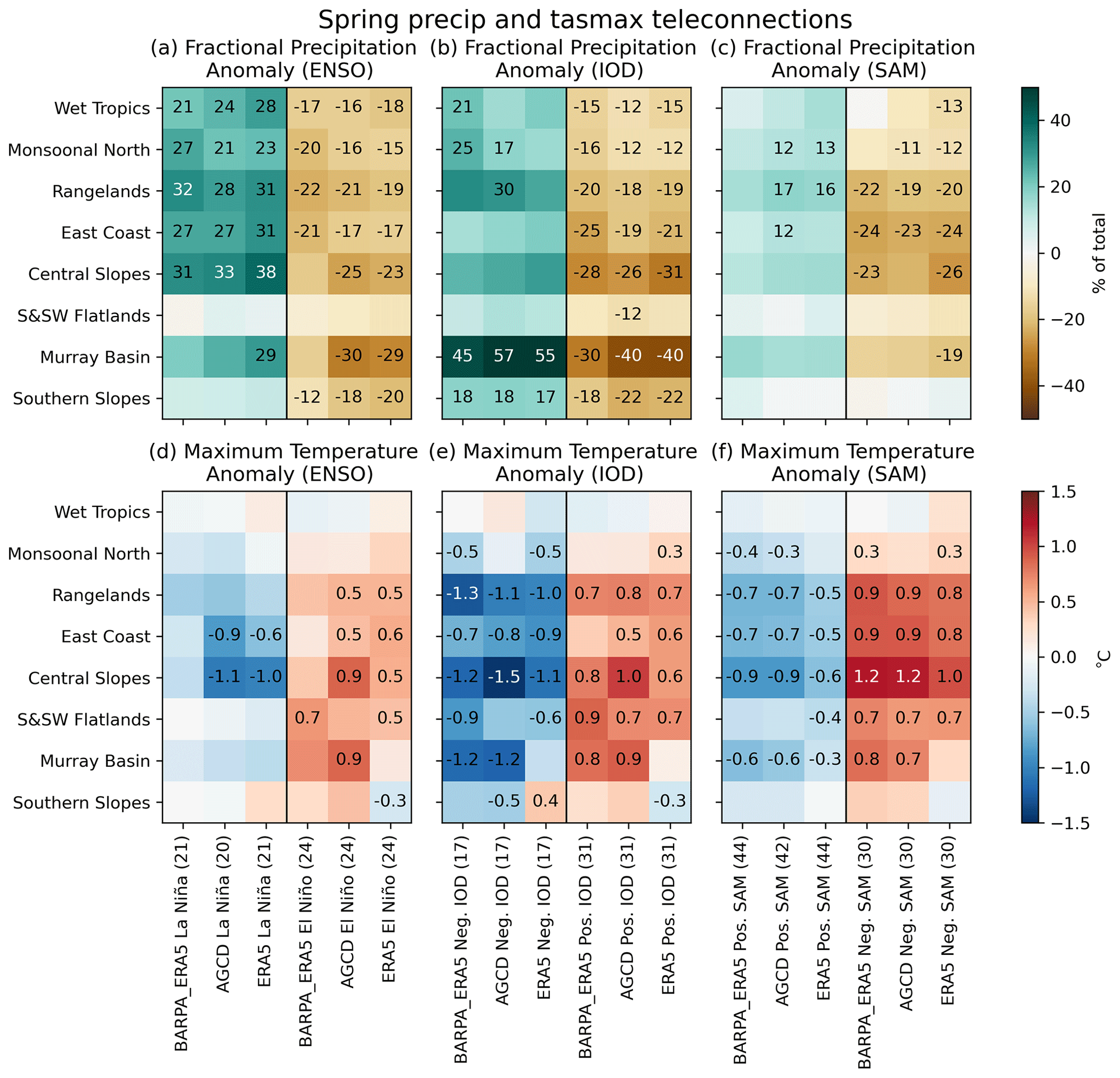
Figure 7 Spring fractional precipitation (a–c) and maximum temperature (d–f) composite anomalies under positive and negative phases of (a, d) ENSO, (b, e) IOD, and (c, f) SAM. Values are annotated on the panels when the composite anomaly is statistically significant from 0 at the p>0.05 level using a Welch's t test.

Figure 7 shows the composite differences between the active phases of each mode of variability and the climatological means for precipitation and daily maximum temperatures, aggregated across the NRM clusters. Precipitation anomalies are presented as percentages of the climatological mean. Spatial variability in the IOD teleconnection is very similar across all three datasets. In the northern clusters, precipitation anomalies during the positive phase of the SAM are too weak in BARPA-R and do not reflect AGCD's statistical significance. BARPA-R also misses significant warm and cool temperature anomalies in the central slopes and East Coast clusters due to both phases of ENSO. However, there is a remarkably close correspondence between maximum temperature and the SAM across BARPA-R and AGCD. Overall, all three teleconnections are well represented by BARPA-R.

3.4 The 10 m winds

In the absence of a gridded wind analysis, near-surface wind speeds have been evaluated against 3-hourly station observations taken from 10 m masts. Where quality information was present, observations that were flagged as wrong, suspect, or inconsistent were excluded from the analysis. Model and reanalysis data corresponding to the observations were extracted from ERA5 and BARPA-R. For each station, instantaneous wind speed data for a height of 10 m a.g.l. were extracted from the nearest grid cell to the station position. The model dynamical time steps (7.5 min for BARPA-R and 12 min for ERA5) roughly correspond to the observational averaging period (10 min), which ensures that the modelled and observed wind speeds are comparable. Only time samples for which valid station data were present are considered. The resulting model and observation data were then aggregated to NRM cluster level.

Resulting quantile–quantile (Q-Q) plots of observed and corresponding modelled 10 m wind speed for each NRM cluster are presented in Fig. 8. The Perkins skill score (PSS Perkins et al., 2007) has been used to compare the distributions of BARPA-R and ERA5 to the observed station wind speeds and is listed in the captions of Fig. 8. The PSS measures the difference between two normalised distributions, ranging between 1 for a perfect match to 0 for no overlap between distributions, and is sensitive to histogram bin width, in this case 0.5 m s⁻¹. In six of the eight NRM clusters, BARPA-R shows an improved PSS and improved 99th percentile wind speeds compared to ERA5. BARPA-R generally shows improved high percentile tail values compared to ERA5, while both models underestimate “calm” weather conditions with wind speeds of 0 m s⁻¹. In the upper tail, there is a general tendency for both BARPA-R and ERA5 to have the Q-Q line tending towards lower values, similar to previous results for BARPA-R downscaling of CMIP5 simulations that also found an improvement for this when using BARPA-C convection-permitting simulations (Dowdy et al., 2021). This is as expected to some degree given the very strong winds from some localised storms may be better simulated at finer scales.

In summary, performance evaluation of precipitation and surface air temperatures has demonstrated that BARPA-R is capable of producing a faithful representation of present-day climate when deriving driving inputs from ERA5. BARPA-R shows a persistent wet bias across a set of precipitation-related indices and a winter cold bias in maximum temperatures. Maximum temperature trends are broadly consistent with observations, while warming trends in minimum temperatures are overestimated. Precipitation trends resemble ERA5 more closely than AGCD, and while the cool-season drying in southern Australia is well captured, deficiencies in simulating the intensification of heavy precipitation by parameterised convection models is evident in both BARPA-R and ERA5. Regional correlations with key modes of variability, namely ENSO, IOD, and SAM, are well simulated. The 10 m winds are improved over ERA5 but still underestimate the high tails of the distribution in many regions.

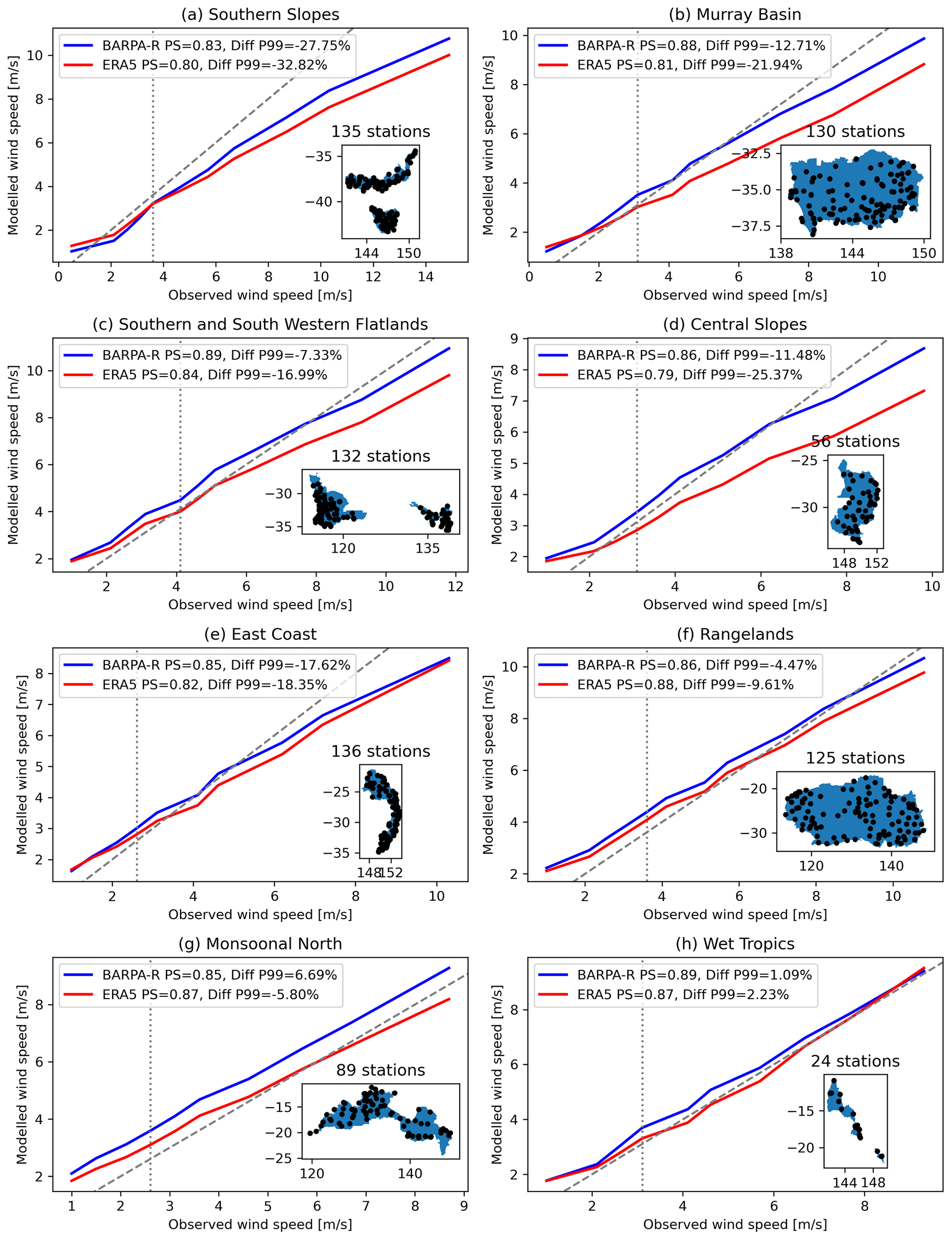
Figure 8 Q-Q plots of observed and modelled hourly wind speeds at station locations in each NRM cluster of ERA5 (red) and BARPA-R (blue) compared to station observations. Perkins skill scores and 99th percentile biases are given in each panel's legend. Station locations are shown as black dots in the inset maps. Model data are derived from time step instantaneous winds and interpolated to station locations using a nearest-neighbour interpolation scheme. The number of stations and hours are given in each panel label.

4 Process evaluation

This section provides an analysis of the BARPA-R's representation of some key atmospheric dynamical and thermodynamical processes that are important for the Australian region. Focus is placed on key wind circulation features and on large-scale weather systems. Firstly, the climatologies of these features are compared between BARPA-R and observational datasets. This climatological analysis is provided to demonstrate the fidelity with which BARPA-R reproduces regional climate process. Secondly, interannual correlations of location and frequency statistics for each circulation feature or weather system are computed between BARPA-R and the real-world observations. This correlation analysis demonstrates the degree to which the weather and circulation is coupled with the boundary conditions versus the degree to which these systems are free to evolve independently within the model.

4.1 Circulation

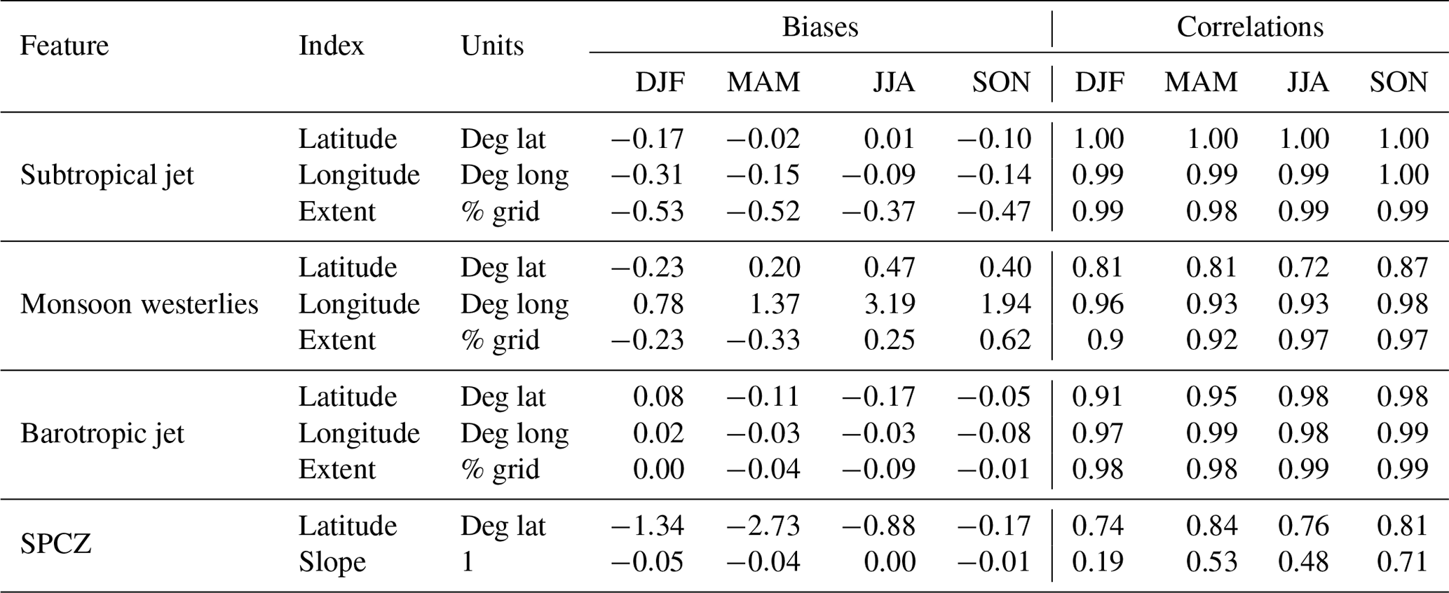
Figure 9 shows heatmaps of the frequency of the presence of three key large-scale circulation features of the Australian region across four seasons: the barotropic and subtropical jets and the monsoonal westerly winds. Table 1 further shows the biases and interannual correlations with ERA5 key properties of each circulation feature. In this analysis, ERA5 is used as the reference dataset. The computational methods apply simple thresholds to daily mean wind speeds to determine the horizontal locations of each circulation feature. The occurrence frequencies are likely to be somewhat sensitive to the choice of thresholds; however, further analysis (not shown) has found that BARPA-R model biases are robust to threshold choice. The location of the South Pacific Convergence Zone is also shown. Feature definitions are given below.

• The barotropic westerly jet (blue) where 850 and 200 hPa zonal winds both exceed 10 m s⁻¹.

• The monsoon westerlies (green) where 850 hPa zonal wind is westerly, while 200 hPa zonal wind is easterly.

• The subtropical jet (red) where 200 hPa zonal winds exceed 30 m s⁻¹.

• The South Pacific Convergence Zone (SPCZ, orange), which shows a linear fit to the latitude of the monthly maximum of precipitation in the southwestern Pacific for each longitude point between 150 and 200^∘ E. This methodology is modified from Brown et al. (2013) for the BARPA-R domain. In Fig. 9, the orange marker indicates the interannual inter-quartile range of the seasonal SPCZ location.

All four features are present in both BARPA-R and ERA5 in Fig. 9, with matching seasonal cycles. Some biases are evident, however, which are further summarised in Table 1. The largest biases are present in the monsoon westerlies, which are shifted too far east, particularly during the boreal monsoon, and the SPCZ, which is shifted south in March to May. The spatial extent of the subtropical jet is additionally reduced in all seasons. The bias in the monsoon westerlies is a persistent systematic MetUM bias (Rodríguez and Milton, 2019). This bias has been linked by Martin et al. (2021) to errors in the representation of convection over the Maritime Continent and the western to central equatorial Indian Ocean. Systematic rainfall biases in the maritime continent are common due to the complex, multi-scale nature of convection in this region. A reduced southerly bias in the SPCZ location has been documented in the ACCESS-S1 seasonal forecast system (Beischer et al., 2021), suggesting that ocean coupling may improve the representation of the SPCZ.

The right-hand side of Table 1 shows the correlations between the circulation system indices (latitude, longitude, spatial extent, and SPCZ slope) in ERA5 and BARPA-R. These correlations are not measures of model performance, as it is not required that BARPA-R shows perfect agreement in interannual variability phasing as its driving model. Instead, they show where circulation systems are influenced by the internal variability of the BARPA-R system and where they are constrained by boundary conditions and sea surface temperature (SST) forcing. From the table, it is evident that tropical features, namely the SPCZ and the monsoon westerlies, have a larger degree of internal variability, while the subtropical and barotropic jets are more constrained and remain in phase with ERA5.

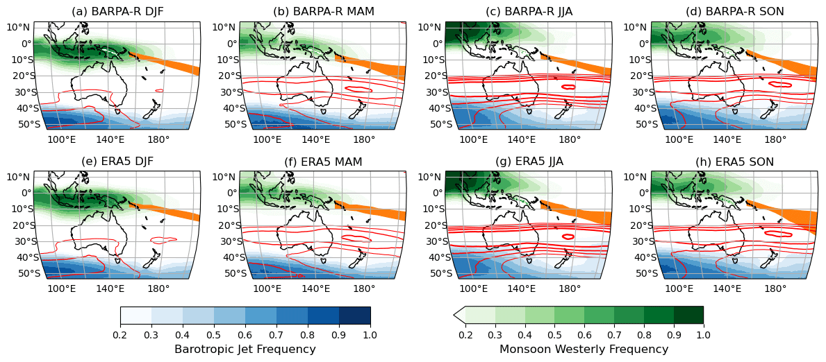
Figure 9 Heatmaps of seasonal circulation feature fractional frequency, ranging from 0 to 1, in BARPA-R (a–d) and ERA5 (e–h). Colours indicate the westerly jet at 850 hPa (blue), the monsoonal westerlies at 850 hPa (green), the subtropical jet at 200 hPa (red lines; contour interval =0.15; first contour: 0.2). Additionally, the location of the SPCZ is shown in orange. Feature definitions are provided in Sect. 4.1.

Table 1 Bias and interannual correlations of circulation features compared to ERA5.

4.2 Weather systems

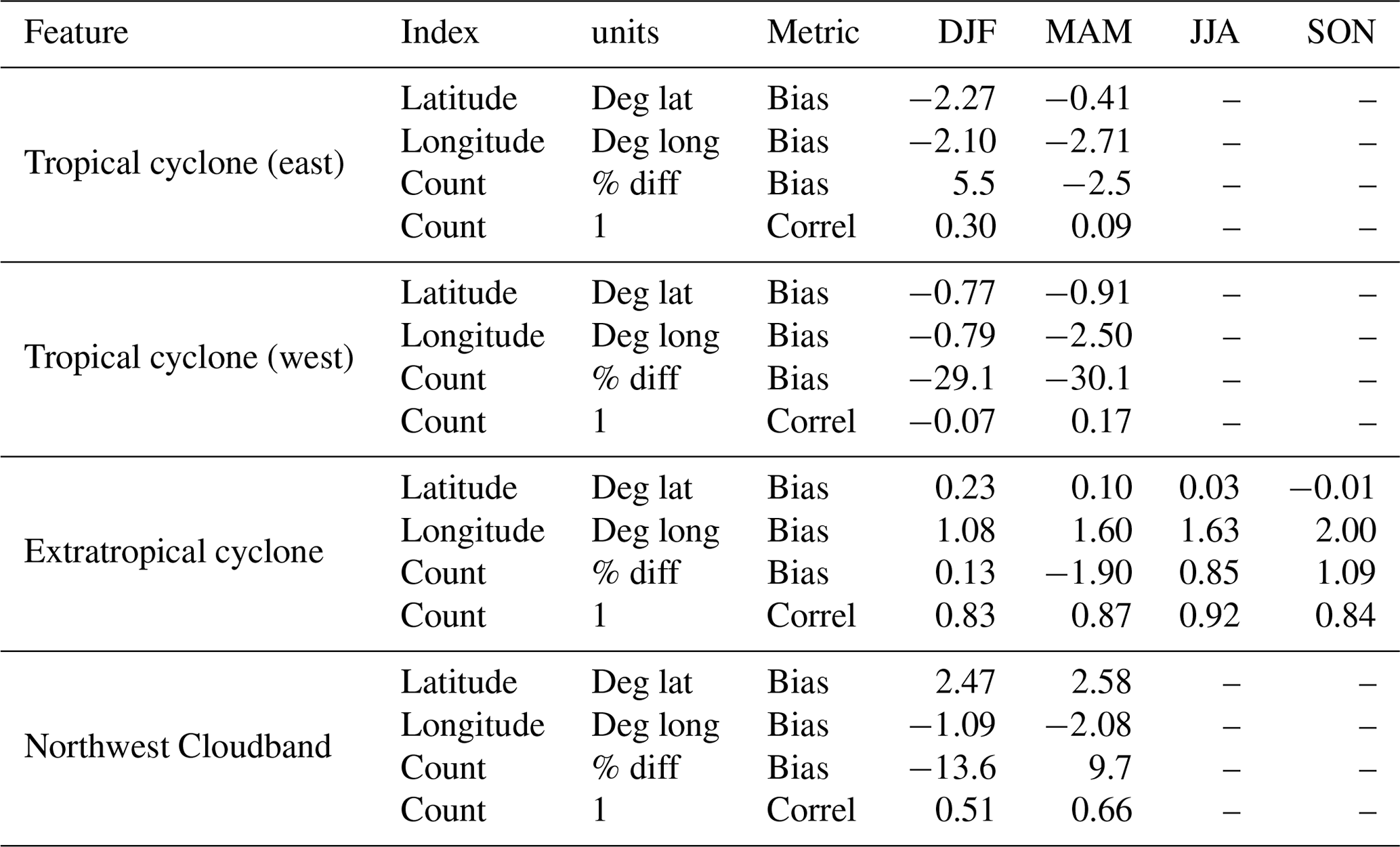
Figure 10 and Table 2 follow the format of Fig. 9 and Table 1 but consider a set of large-scale weather systems that influence Australia, namely tropical and extratropical cyclones, and Australian Northwest Cloudbands (NWCBs). Where weather features only occur in limited seasons are not necessarily observed in every year, interannual correlations are only given for the feature counts, and statistics are only shown in seasons when the weather systems are present. In this analysis, some direct observational products are available, and these are used as references where possible. Where no direct observation is available, ERA5 is used as the reference. Identification algorithms and reference datasets are described below.

Firstly, tropical cyclones are identified using the Okubo–Weiss–Zeta (OWZ) methodology following the methodology of Tory et al. (2013) and Bell et al. (2018). This algorithm uses a low-deformation vorticity parameter derived from vorticity and deformation parameters at 850 and 500 hPa, and tropical cyclone environment parameters derived from relative and specific humidity at 950 and 700 hPa. The reference dataset is the International Best Track Archive for Climate Stewardship (IBTrACS Knapp et al., 2010). In Table 2, tropical cyclones are split into eastern and western systems along the longitude band at 135^∘ E, corresponding to the Indian Ocean and western Pacific Ocean tropical cyclone basins. Secondly, extratropical cyclones are identified using the University of Melbourne (UM) tracker (Pepler and Dowdy, 2021) by identifying local minima in mean sea level pressure for which the maximum sea level pressure Laplacian exceeds 0.8 hPa deg lat⁻² and which originate south of 35^∘ S. In this case, tracks derived with the same algorithm using ERA5 reanalysis are used as the reference dataset.

Finally, NWCBs are identified using the MetBot (Hart et al., 2012). This algorithm identifies bands of continuous low daily outgoing longwave radiation (OLR) spanning from the tropics through the subtropics and has been used to identify similar weather systems in southern Africa and South America. In this Australian application, the OLR threshold has been set to 240 K in observations and 255 K in BARPA-R, with the latter selected through matching quantiles of daily OLR. Each NWCB must intersect the longitude range 110–155^∘ E along each latitude band between 29 and 11^∘ S.

Together, Fig. 10 and Table 2 show that extratropical cyclones are well represented in BARPA-R across all seasons. There is a westward bias in feature locations and high correlations above 0.8 across BARPA-R and the ERA5-based reference. Tropical cyclones are generally shifted south and west, and the large spike in cyclone systems in northwestern Australia is underestimated. Tropical cyclone interannual variability is decoupled from observations, with very low and even negative correlation values present. Further investigation (not shown) indicates that tropical cyclone locations and paths diverge on seasonal and sub-seasonal timescales between BARPA-R and observations away from the domain boundaries. Finally, the spatial distribution of NWCBs has the correct shape, with a maximum over the Australian East Coast in the DJF season. However, cloud band counts are reduced by 13 % in this core NWCB season. Interannual correlations with observations are 0.5 and 0.66 in DJF and MAM, respectively, suggesting a degree of coupling with the boundary conditions as well as real-world interannual variability.

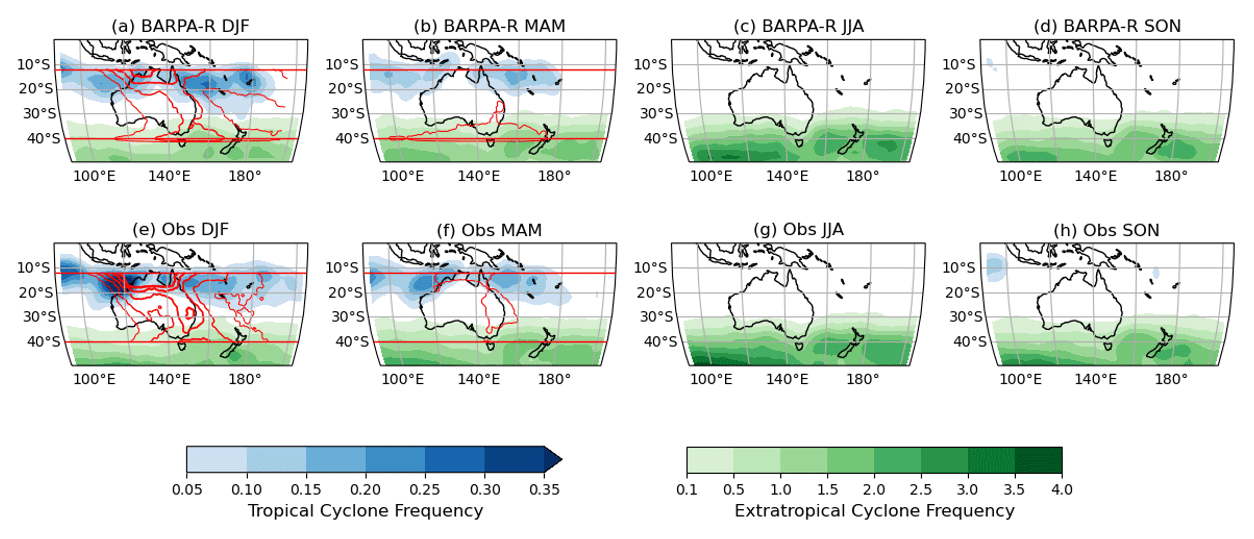
Figure 10 Heatmaps of seasonal weather feature frequency, in units of events per square degree per season, in BARPA-R (a–d) and observations (e–h). Colours indicate tropical cyclones (blue), extratropical cyclones (green), and NWCBs (red lines; contour interval: 1 event/season; starting value: 2). Feature definitions are provided in Sect. 4.2. Observational products vary by feature: IBTRaCS tropical cyclones, ERA5 extratropical cyclones, and NOAA satellite-derived daily OLR-based cloud bands.

Table 2 Bias and interannual correlations of weather features compared to IBTRaCS, ERA5 and NOAA OLR as per text.

5 Lagged temperature–precipitation relationship

Correct simulation of multivariate relationships between RCM output variables are important for accurately representing weather processes, compound events, and downstream impact modelling, which take multiple inputs from RCMs (Kim et al., 2021, 2023; Sain et al., 2011). Therefore, it is important to assess how well BARPA-R captures multivariate relationships, particularly between key variables like temperature and precipitation, as compared to existing observational and reanalysis datasets.

A useful metric for characterising the relationship between two variables is their time-lagged correlation, which can indicate how each variable responds to anomalies of the other through examination of positive and negative lags, respectively. Hence, the lagged correlations between these variables may be useful to examine the time lag and determine the strength and direction of the relationship between them (Kumar et al., 2013). At longer timescales, lagged correlations can also be helpful to identify potential feedback mechanisms between precipitation and temperature. For instance, if increased precipitation leads to cooler temperatures, this can lead to enhanced vegetation growth, which can further increase precipitation due to amplified transpiration and evaporation. In convective climates, positive correlations at negative lags may be linked with atmospheric instability as the land heats up, thus making conditions favourable for convection to occur, while negative correlations at positive lags suggest that the precipitation cools the surface due to evaporation and cloud cover, resulting in lower temperatures. Moreover, positive correlations at positive lags (especially in the minimum temperatures) may be associated with increased cloudiness, thereby increasing the chances of instability and precipitation; additionally, an increase in warm and humid conditions is expected, leading to higher temperatures.

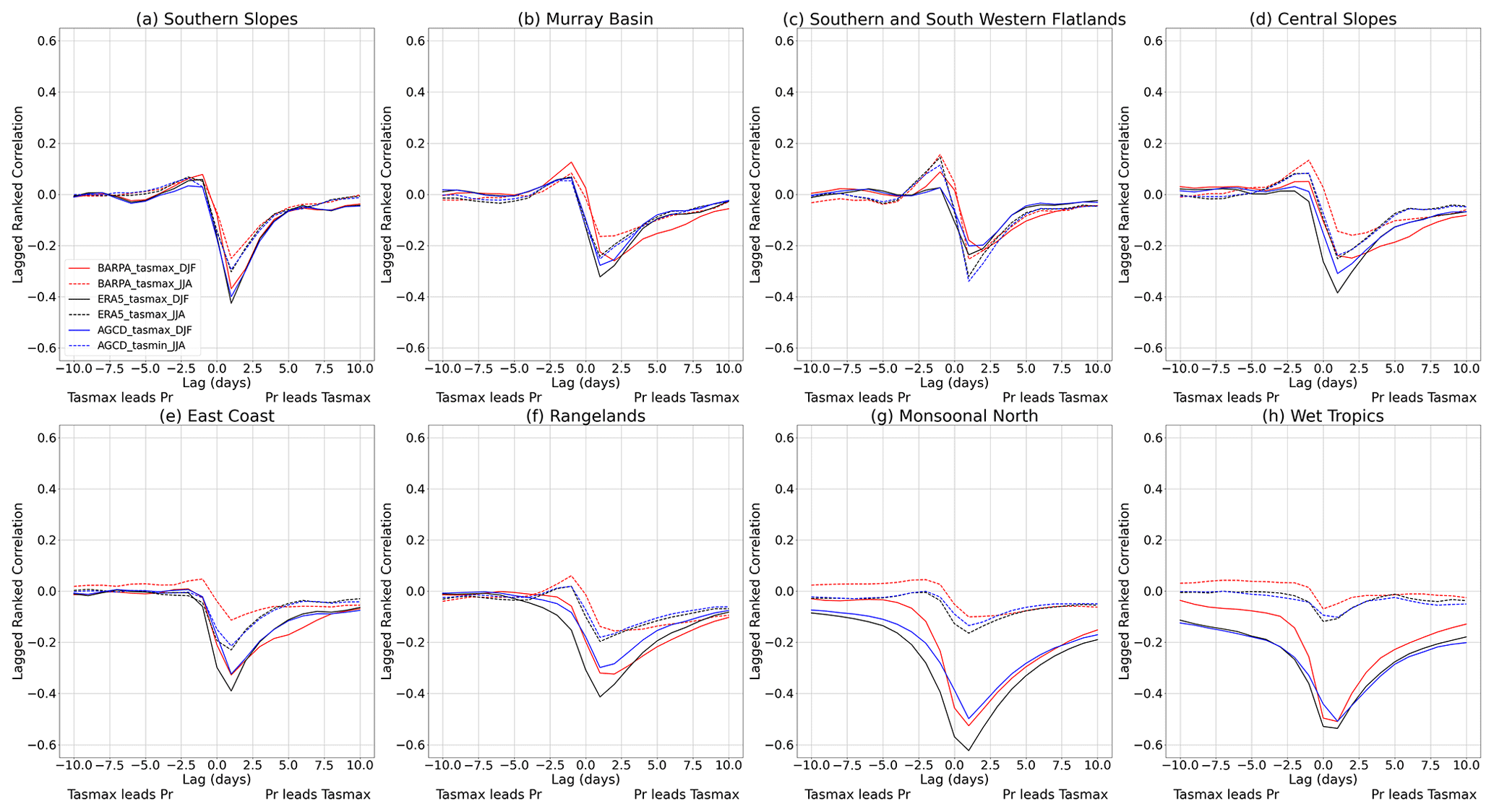
Figure 11 Lagged Spearman ranked correlations between daily precipitation and maximum temperature (tasmax). Lines indicate BARPA-ERA5 (red), ERA5 (black), and AGCD (marked in blue) in DJF (solid lines) and JJA (dashed lines) over the eight NRM clusters across Australia (as labelled). Daily AGCD and modelled precipitation data are set to zero where the values are less than (<) 1 mm d⁻¹. The correlation is computed at each grid point, before being spatially averaged over each region.

This section evaluates the daily temperature–precipitation relationship in BARPA-R and compared to AGCD and ERA5. Seasonal Spearman ranked correlations with lag time of ±10 d are computed between the daily maximum and minimum temperature and precipitation outputs from 1985 to 2014. A lower precipitation threshold of 1 mm d⁻¹ was applied before ranking the precipitation data to remove sensitivity to data storage precision. Incorporating a precipitation threshold of 1 mm d⁻¹, assuming that this is the minimum amount of precipitation required to be considered a precipitation event for a particular day. The time steps of AGCD maximum temperature data were shifted by 1 d to ensure that valid times were consistent across all datasets.

Figures 11 and 12 show the lagged Spearman ranked correlations between daily precipitation and near-surface minimum and maximum temperatures (tasmin and tasmax) in the different datasets: namely, BARPA-R, ERA5, and AGCD in DJF and JJA over the eight NRM clusters. The remaining seasons showed similar results (not shown). The lagged temperature–precipitation correlation relationships between ERA5 and AGCD are very similar across seasons and NRM clusters.

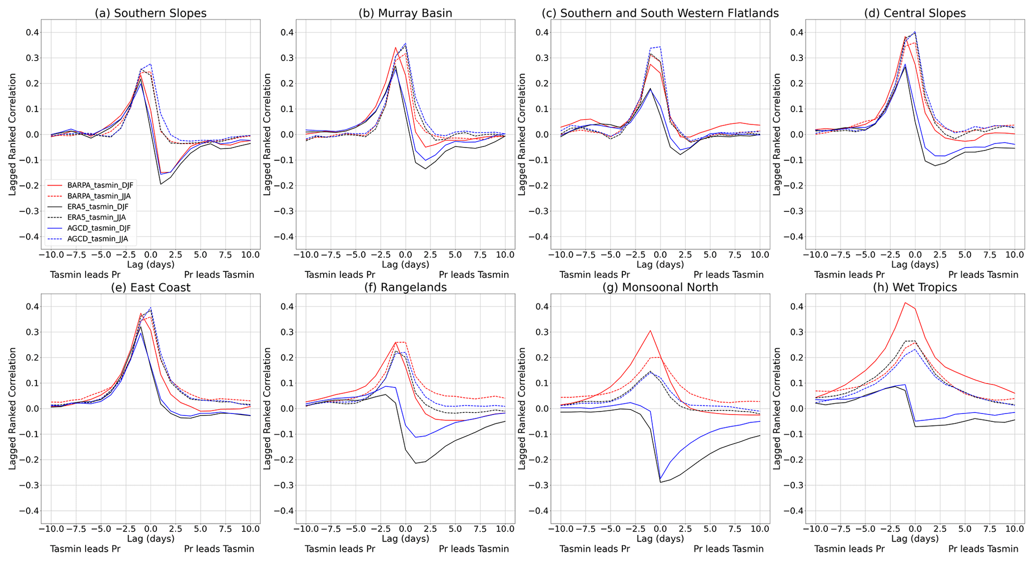
Figure 12 Lagged Spearman ranked correlations between daily precipitation and minimum temperature (tasmin). Lines and subplots as per Fig. 11.

In the mid-latitude regions (Fig. 11a–e), precipitation generally leads tasmax with negative correlation at positive lag of around 1 d, suggesting that precipitation initially cools the surface, leading to lower maximum temperature. This is consistent across all three datasets in all seasons. In all three datasets and in both seasons, tasmin leads precipitation (Fig. 12a–e) with positive correlation at negative lag of around 1 d (which may accelerate evaporation, leading to an increase in atmospheric moisture and condensation). Seasonal differences in the tasmin–precipitation relationship are well distinguished by BARPA-R in the southern slopes, Murray basin, and SSW flatlands regions, while in the central slopes (Fig. 12d) and East Coast (Fig. 12e) the BARPA-R DJF relationships more closely resemble the observed relationships in JJA.

In northern central Australia, the observed precip–tasmin relationship is distinctly different between DJF and JJA (Fig. 12f–h). In JJA, this relationship is characterised by positive correlations and is well simulated by BARPA-R. However, in DJF, negative correlations are seen at a positive lag of around 1 d in both AGCD and ERA5. However, BARPA-R still shows positive correlations at negative lag (Fig. 12f–h), resembling its relationship in JJA. In these regions, namely, the rangelands, monsoonal north, and wet tropics, BARPA-R shows a substantially different minimum temperature–precipitation relationship to AGCD and ERA5. This suggests that in the aforementioned regions (Fig. 12f–h) BARPA-R is unable to perform well relative to AGCD and ERA5 and does not reproduce the observed daily minimum temperature–precipitation relationship in the DJF season (Fig. 12f–h). BARPA-R performs considerably better at simulating the observed precip–tasmax relationship in northern Australia (Fig. 11g, h), resolving the strong seasonal differences between DJF and JJA apparent in the monsoonal north and wet tropics. In these regions, the DJF correlations are strongly negative, with maximum values between −0.55 and −0.65.

The maximum strength of the correlations between precipitation and minimum or maximum temperature between the two variables is generally quite strong (±0.3–±0.4) in the NRM clusters for all the datasets. The strongest correlation (±0.6) between precipitation and maximum temperature is observed in DJF season over the monsoonal north and wet tropics in all the datasets. In all other regions, BARPA-R precipitation is more sensitive to minimum temperature in the summertime (DJF) relative to AGCD and ERA5; hence, BARPA-R shows a slightly larger magnitude in correlations (with all peaking about zeroth lag). Further results can be found in the Appendix where the spatial maps of Spearman's ranked correlation coefficients at lag 0 between the daily precipitation and minimum temperature outputs from 1985–2014 are shown (Figs. A4 and A5) in DJF and JJA in the BARPA-R, AGCD, and ERA5 datasets.

Overall, BARPA-R simulates realistic relationships between daily maximum temperatures and precipitation across all NRM clusters and in both seasons. Relationships between daily minimum temperatures and precipitation are also well simulated in mid-latitude regimes, namely during winter, and across southern Australia. In convective regimes, such as northern and central Australia and to a lesser extent along the East Coast, a shift in the minimum temperature–precipitation relationship is apparent in observational datasets but not reflected in BARPA-R. Instead, the BARPA-R JJA relationship persists into DJF in these clusters. These conclusions are consistent with spatial maps of the zero-lag correlations provided in Figs. A4 and A5.

The skilful representation of multivariate relationships has implications for the interpretation of climate risk assessments of compound weather events. For example, hot and dry conditions may lead to enhanced bushfire risk, while hot and humid conditions are associated with enhanced heat stress on humans and livestock. In regions where models struggle to represent correct multivariate relationships, simulations of compound events may be adversely impacted. Improvements to the representation of atmospheric convection, either through improved parameterisation or explicit simulation, may improve the minimum temperature precipitation relationship in the northern Australian wet season.

6 Discussion and conclusions

This paper has analysed the ability of the BARPA-R RCM to maintain a realistic Australian climate when driven with ERA5 reanalysis. Performance in the simulation of Australian temperatures and precipitation was found to be frequently on par with and sometimes improved on the ERA5 reanalysis, despite the contribution of data assimilation in ERA5. This analysis considered mean state biases, seasonality, and interannual variability of key ICCLIM metrics chosen to describe the temperature and precipitation climates in the Australian region. Precipitation and temperature teleconnections of the SAM, ENSO, and IOD were shown to be well captured by BARPA-R when the appropriate circulation signals are present in the driving boundary inputs and sea surface temperatures. Contemporary change signals of warming were present and, in many cases, overestimated in BARPA-R, while contemporary wetting signals in northern Australia were underestimated.

Key mean state biases that exceeded those present in ERA5 included JJA cold biases in daily maximum temperatures of around 1 ^∘C across the southern NRM clusters and JJA warm biases in daily minimum temperatures, together leading to a reduced cold-season diurnal temperature range. These JJA temperature biases are also evident in MetUM-based regional reanalyses (Su et al., 2023). The mean monthly maximums in daily precipitation were overestimated by 2–12 mm d⁻¹ across all NRM clusters in both summer and winter. DJF rain day counts were improved in northern regions compared to ERA5 but degraded in southern regions. The simulation of near-surface wind speeds was improved compared to ERA5, but nevertheless underestimated the tail of the distribution in all but the two northernmost NRM clusters.

BARPA-R shows improvements in mean state biases over Australia when compared to the previous generation of RCMs, namely CORDEX-CMIP5 (Di Virgilio et al., 2019b) and the ESCI prototype BARPA-R simulations (Su et al., 2021). The pronounced June–August maximum temperature cold bias, which ranged from −2 to −5 ^∘C in CORDEx-CMIP5, is substantially reduced to −1.1 ^∘C in BARPA-R. The mean state East Coast precipitation bias is reduced but remains substantial with an overall DJF mean of 10 mm d⁻¹. The bias in the number of overall rain days is reduced in the DJF season from values of up to 5 extra days per month in the ESCI-BARPA simulations to 1–2 extra days across all NRM clusters in BARPA-R. Meanwhile, the ESCI-BARPA underestimation of heavy rain day frequency by 1.5–2 d in the wet tropics is transformed to a 0.1 d positive bias in BARPA-R. These changes are likely to be attributable to the inclusion of the improved, “prognostic entrainment” convection scheme in the new version (Su et al., 2022b).

As BARPA-R projections are intended to produce hazard information for risk assessment purposes, it is important that BARPA-R is able to simulate correct frequencies of hazard-relevant weather and circulation systems. As a first attempt at analysing this, Sect. 4 focused on the representation of key circulation and large-scale weather systems, such as tropical cyclones, extratropical cyclones, and monsoon westerlies. All circulation and weather systems analysed were present with accurate seasonal cycles in BARPA-R. This is a reassuring but expected result, given that the length scales of the systems are large and that these systems are well represented in the driving datasets. Future investigations into the representation of finer-scale systems such as sea breeze circulations, dry lines, and mountain meteorology may yield more insightful findings. In general, tropical systems such as the monsoon westerlies, tropical cyclones, and the Northwest Cloudbands showed larger biases in location and frequency statistics than extratropical systems such as extratropical cyclones. These tropical systems also showed less correlation on interannual timescales than extratropical systems. This has implications for future experiment design on hazard analysis. While a case study approach comparing BARPA-R with its driving model may be appropriate for studying extratropical systems in some instances, it is unlikely to be practical for tropical systems due to the divergence between driving and downscaling model behaviour. A larger sample size may therefore be required, especially for studies of rare events such as tropical cyclone landfall.

Both BARPA-R and ERA5 underestimate the intensification trend of wet-day precipitation (SDII) observed in AGCD. This result is consistent with global studies of atmospheric models with parameterised convection and has been found elsewhere to be rectified by the explicit representation of atmospheric convection (Fowler et al., 2021; Lee et al., 2022; Luu et al., 2022). This is particularly true for subdaily rainfall, which has not been evaluated in this paper. Further downscaling of both climate projections and regional reanalysis to convection-permitting length scales over the Australian region are therefore necessary for the assessment of changes in high-intensity, short-duration rainfall (Wasko et al., 2023).

Many of the biases and limitations in BARPA-R identified by this study are common biases of the MetUM. These include the overall wet bias (Hudson et al., 2017), the overestimation of the monsoon westerlies (Martin et al., 2021), and the reduced diurnal temperature range in winter (Su et al., 2023). Future development of BARPA-R will take advantage of ongoing MetUM model development, such as the inclusion of the CoMorph convection scheme and updates to the JULES land surface model, with the potential of improving these model shortcomings going forward.

This paper has demonstrated that BARPA-R is able to downscale ERA5 reanalysis to produce a reasonable climate over Australia. This evaluation experiment meets the CORDEX requirement to downscale ERA5 reanalysis in order to evaluate RCM performance in the absence of biased GCM-based driving inputs. Having shown good performance in the evaluation experiment, GCM-based downscaling with BARPA-R is now underway. This BARPA-GCM ensemble will require additional evaluation and is not guaranteed to show similar performance over the Australian region. If key planetary-scale model circulations and processes, such as ENSO or the subtropical jet, are biased or missing in the driving GCM, BARPA-R is unlikely to be able to compensate for these errors. Additionally, non-linear errors may arise from incompatibility between driving GCMs and the downscaling BARPA-R GCM, such as if the two models have very different favoured vertical profiles of temperature or humidity.

Further work will perform a broader evaluation of BARPA-R's performance at downscaling both ERA5 and CMIP6 GCMs. Benchmarking of the performance of BARPA-R and other CORDEX-CMIP6 RCMs at downscaling historical experiments is needed to establish the credibility of their downscaled projections. The added value of RCMs over GCMs must be evaluated in order to assess the value of computationally expensive dynamical downscaling going forward. Hazard-specific evaluations are required to understand the representation of hazards in BARPA-R simulations before these simulations may be used for risk assessment. Following this evaluation of the full BARPA-R system, these simulations will provide hazards intelligence and climate services to support and inform decision-making.

Appendix A: Supplementary Figures

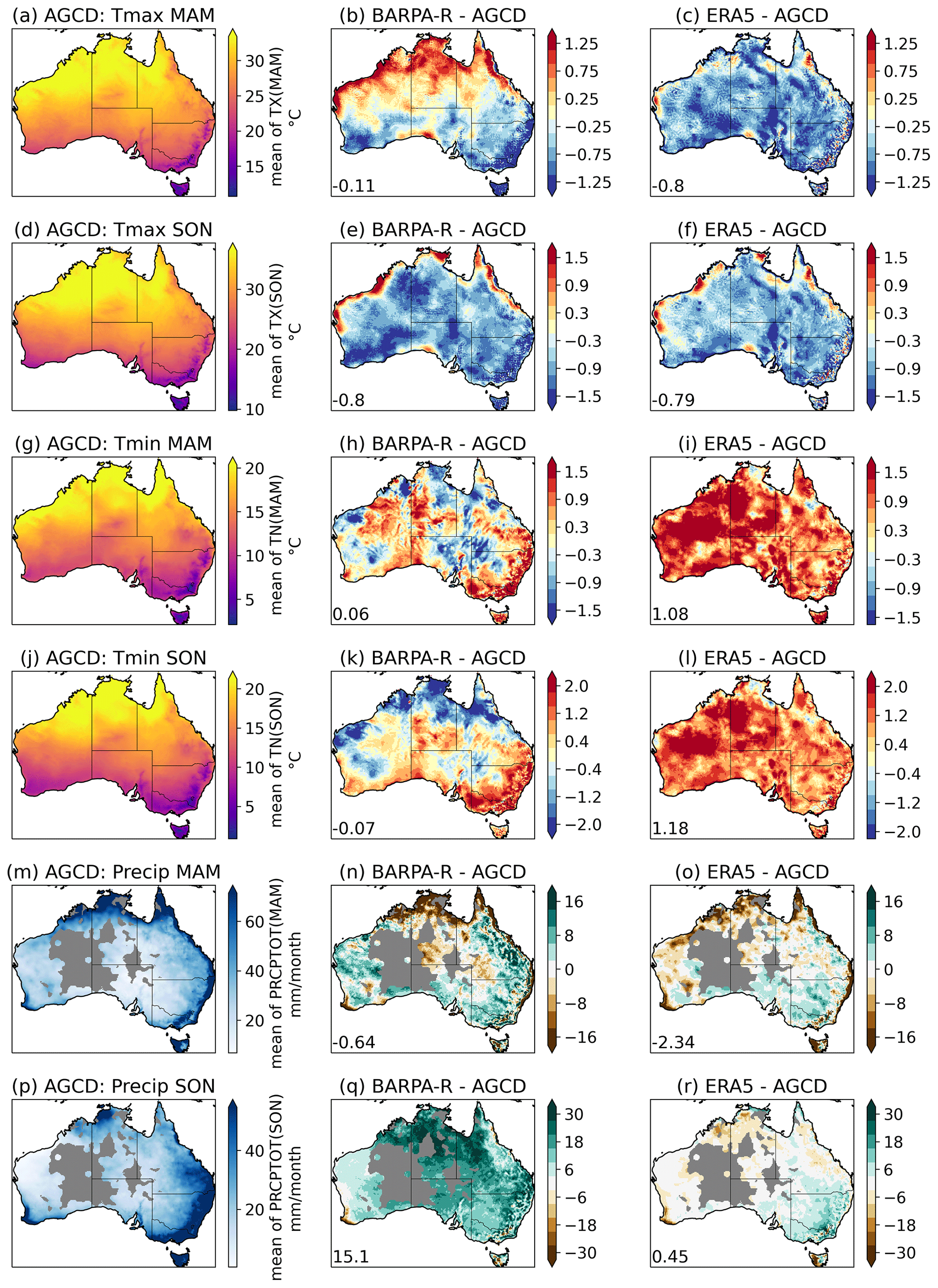
Figure A1 Bias in temperature and precipitation climate indicators (rows: TX, TN, and PRCPTOT) for transition seasons MAM and SON for BARPA-R and ERA5 (second and third columns) against AGCD (first column) averaged across the core evaluation period (1985–2014).

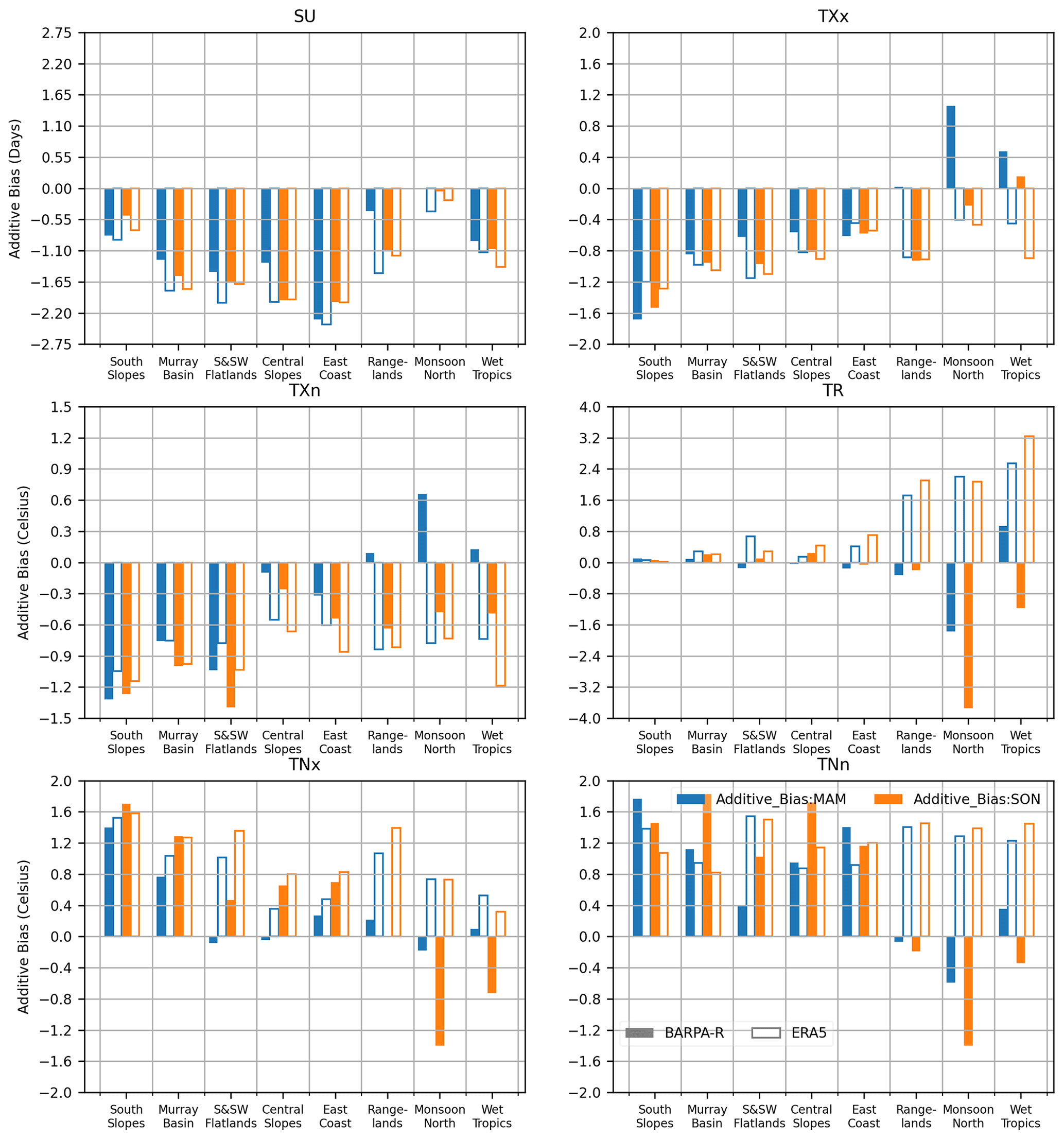
Figure A2 BARPA-R (solid bars) and ERA5 (outlined bars) transition season biases of six temperature indices across the eight Australian NRM clusters. Reference data are sourced from AGCD. Panels show the number of summer days, (SU; with daily maximum temperatures exceeding 25 ^∘C), tropical nights, (TN; with daily minimum temperatures exceeding 20 ^∘C), and the monthly minimums and maximums of the daily minimums and maximums (TNn, TNx, TXn, and TXx). Blue and orange bars show the bias aggregated over austral autumn and spring, respectively.

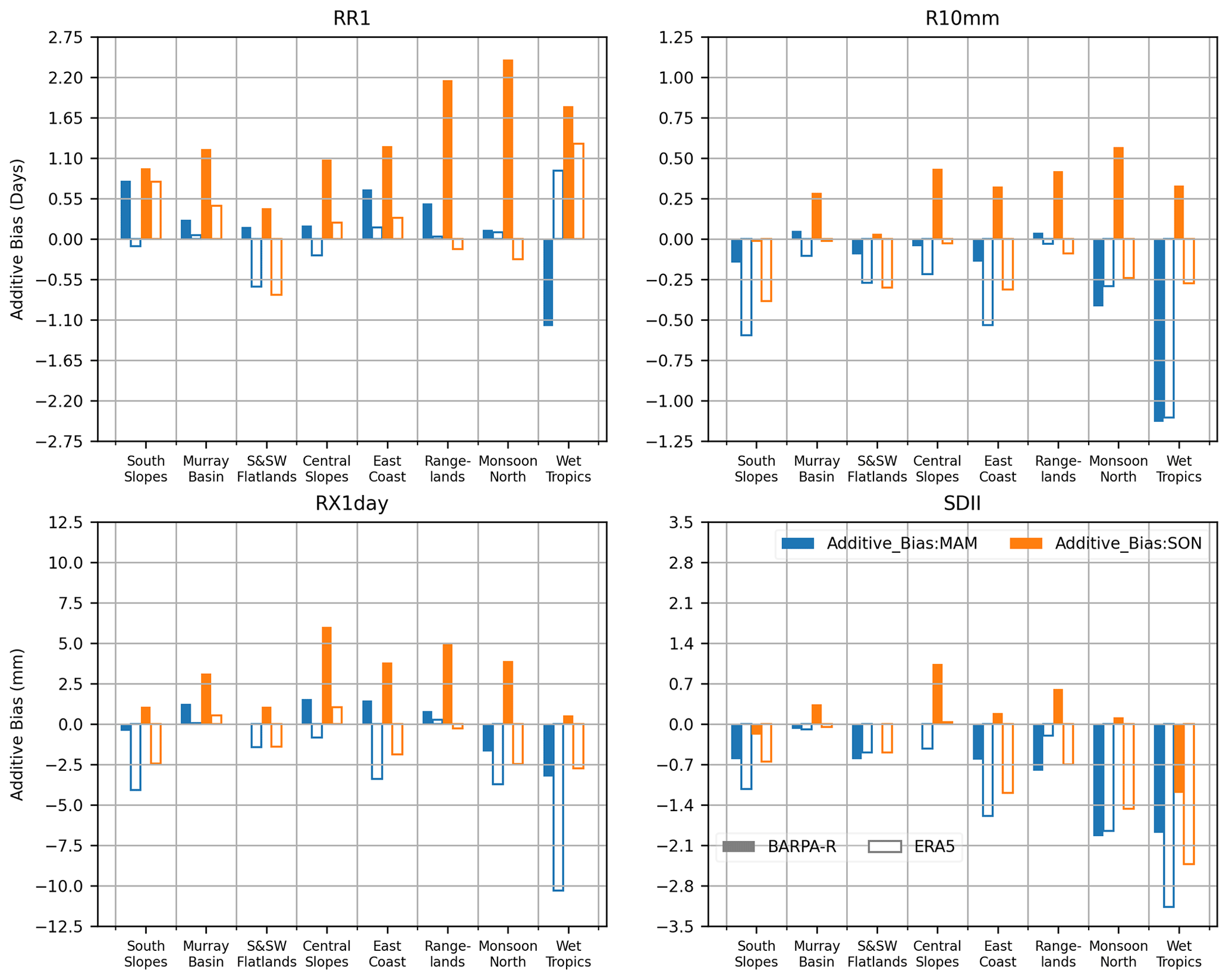
Figure A3 As per Fig. A2 but for precipitation indices: wet days (RR1; >1 mm d⁻¹), heavy rain days (R10mm; >10 mm d⁻¹), monthly maximum daily precipitation (RX1Day), and the overall monthly precipitation (PRCPTOT).

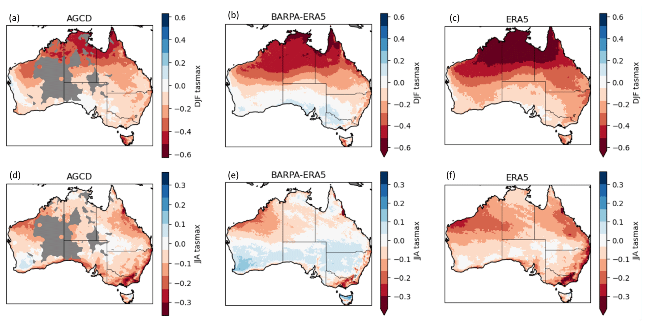
Figure A4 Spatial maps of Spearman's ranked correlation coefficients between the daily precipitation and maximum temperature in DJF and JJA in BARPA-ERA5, AGCD, and ERA5 datasets.

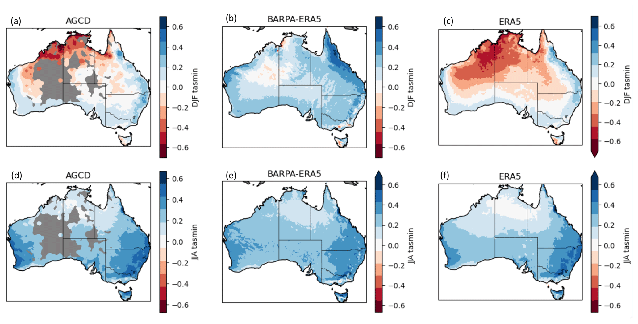
Figure A5 Spatial maps of Spearman's ranked correlation coefficients between the daily precipitation and minimum temperature in DJF and JJA in BARPA-ERA5, AGCD, and ERA5 datasets.