the Creative Commons Attribution 4.0 License.
the Creative Commons Attribution 4.0 License.
 | 26 Sep 2024
Deep dive into hydrologic simulations at global scale: harnessing the power of deep learning and physics-informed differentiable models (δHBV-globe1.0-hydroDL)
Dapeng Feng
Hylke Beck
Jens de Bruijn
Reetik Kumar Sahu
Yusuke Satoh
Yoshihide Wada
Jiangtao Liu
Kathryn Lawson
Accurate hydrologic modeling is vital to characterizing how the terrestrial water cycle responds to climate change. Pure deep learning (DL) models have been shown to outperform process-based ones while remaining difficult to interpret. More recently, differentiable physics-informed machine learning models with a physical backbone can systematically integrate physical equations and DL, predicting untrained variables and processes with high performance. However, it is unclear if such models are competitive for global-scale applications with a simple backbone. Therefore, we use – for the first time at this scale – differentiable hydrologic models (full name δHBV-globe1.0-hydroDL, shortened to δHBV here) to simulate the rainfall–runoff processes for 3753 basins around the world. Moreover, we compare the δHBV models to a purely data-driven long short-term memory (LSTM) model to examine their strengths and limitations. Both LSTM and the δHBV models provide competitive daily hydrologic simulation capabilities in global basins, with median Kling–Gupta efficiency values close to or higher than 0.7 (and 0.78 with LSTM for a subset of 1675 basins with long-term discharge records), significantly outperforming traditional models. Moreover, regionalized differentiable models demonstrated stronger spatial generalization ability (median KGE 0.64) than a traditional parameter regionalization approach (median KGE 0.46) and even LSTM for ungauged region tests across continents. Nevertheless, relative to LSTM, the differentiable model was hampered by structural deficiencies for cold or polar regions, highly arid regions, and basins with significant human impacts. This study also sets the benchmark for hydrologic estimates around the world and builds a foundation for improving global hydrologic simulations.
- Article
(4810 KB) - Full-text XML
- BibTeX
- EndNote


Hydrologic models are vital tools to model and elucidate the terrestrial water cycle, and they have been widely used in flood forecasting (Maidment, 2017), water resource management (Jayakrishnan et al., 2005), and assessing climate change impacts (Hagemann et al., 2013). Recently, deep learning (DL) models have demonstrated superior performance compared to traditional process-based hydrologic models in accurately predicting different components of the hydrologic cycle (Shen, 2018), such as soil moisture (Fang et al., 2017, 2019; Fang and Shen, 2020), streamflow (Feng et al., 2020; Konapala et al., 2020; Kratzert et al., 2019b; Liu et al., 2024), snow water equivalent (Cui et al., 2023; Song et al., 2024c), groundwater (Wunsch et al., 2021), and water quality (Hansen et al., 2022; Rahmani et al., 2021; Saha et al., 2023; Song et al., 2024a; Zhi et al., 2021). Long short-term memory (LSTM) networks, which are a type of recurrent neural network (Hochreiter and Schmidhuber, 1997), and transformers (Vaswani et al., 2017) are currently popular DL algorithms for handling time series dynamics in hydrology, while other architectures can also be employed. LSTM models have established state-of-the-art accuracy for streamflow prediction at continental and smaller scales (Feng et al., 2020, 2021; Kratzert et al., 2019a, b; Lees et al., 2021; Mai et al., 2022).
Although DL models have shown great prediction accuracy compared to traditional models, they usually do not possess clear physical constraints inside the model and are often regarded as “black boxes” despite some recent interpretive efforts (Lees et al., 2022). Thus, purely data-driven models are limited in that they cannot predict unobservable or untrained physical variables, which impedes the investigation of the physical relations of different hydrologic variables behind the change in the target variable. They may also become overfitted and acquire incorrect sensitivities to inputs (Reichert et al., 2024). In contrast, traditional process-based hydrologic models following physical laws like mass balances can provide a full set of diagnostic outputs for hydrologic variables like soil water storage, groundwater recharge, evapotranspiration, and snow water equivalent, even though they are usually only calibrated on discharge observations (Burek et al., 2020; Müller Schmied et al., 2014). The multivariate output nature of these models provides an opportunity for calibration on one or more observable variables to better predict other, perhaps unobservable, variables (in reality, whether this is the case or not depends on if the issue of parameter non-uniqueness is addressed). However, it seems quite difficult for the traditional physical model to approach the performance level of the DL models in daily hydrograph metrics (Feng et al., 2020; Kratzert et al., 2019b) or to improve in generalization with increasing training data (Tsai et al., 2021). In addition, traditional calibration is typically done site by site and can be time- and labor-intensive. Therefore, it logically follows that integrating DL and process-based models might enable harnessing their respective strengths while circumventing their weaknesses (Shen et al., 2023).
By combining a physical model with a DL model, differentiable modeling (Feng et al., 2022a; Shen et al., 2023) provides a systematic solution to leveraging the strengths of both model types while circumventing their limitations. In differentiable models, we use process-based models as a backbone and insert neural networks to either provide parameters (Tsai et al., 2021) or process substitutes for physical models (Aboelyazeed et al., 2023; Feng et al., 2022a, 2023; Höge et al., 2022; Jiang et al., 2020), or they could use limited physical constraints (Kraft et al., 2022). They are collectively called “differentiable models” in the sense that they can rapidly compute gradients of outputs with respect to inputs or parameters using automatic differentiation (or any other means). The differentiability enables the training of neural network components placed anywhere in the model via backpropagation. Inserting neural networks into process-based models can be perceived as posing questions regarding some uncertain relationships given some known ones (priors), and we want to get answers for these questions by automatically learning from big data.
Some of our recent work involved applying differentiable modeling to the conceptual hydrologic model named Hydrologiska Byråns Vattenbalansavdelning (HBV) (Bergström, 1976, 1992; Seibert and Vis, 2012) and building a physics-informed hybrid model for basins in the contiguous United States (CONUS) (Feng et al., 2022a, 2023). The model is “regionalized” in the sense that the embedded neural network components are trained simultaneously on all basins in the study region in order to provide physical HBV parameters which are learned from raw information of basin attributes, resulting in improved generalizability and reduced overfitting to local noise. With the help of differentiable modeling to flexibly evolve the original structure of HBV, the differentiable hybrid models can approach the performance level of the LSTM model whilst being constrained to physical laws and keeping process clarity to predict untrained diagnostic variables with decent accuracy (Feng et al., 2022a). Since the framework is regionalized, this differentiable model can be used to predict in ungauged regions, and it even extrapolates better spatially than LSTM in data-sparse regions when tested across the CONUS (Feng et al., 2023).
Owing to the complexity of calibration, current global hydrologic models are largely either uncalibrated (Hattermann et al., 2017; Zaherpour et al., 2018) or only calibrated on mean annual water budgets or in limited regions (Burek et al., 2020; Müller Schmied et al., 2014). Only very limited studies attempt to calibrate global models on monthly discharge variations (Werth and Güntner, 2010). We desire efficient regionalized models that maximally leverage available information and provide accurate predictions on diverse basins across different climate groups and geographic characteristics in the world. We also want the models to perform decently even in data-sparse regions, showing competitive extrapolation ability, given that many large regions such as in Africa and Asia lack publicly available streamflow data. DL and differentiable models seem plausible candidates for such simulations. Nevertheless, previous studies on DL and physics-informed differentiable models mainly focus on continental or smaller scales, with a relatively homogeneous forcing dataset – it is unclear if their observed strengths, e.g., high performance and strong generalization ability, can carry over to global scales, where the climate is much more diverse and datasets differ widely in their biases and uncertainty characteristics. In particular, we want to thoroughly examine how well these models can leverage information learned on data-rich continents to characterize the hydrologic processes in ungauged regions across the world. Meanwhile, DL models also show favorable scaling relationships (or “data synergy”), where more data leads to more robust models (Fang et al., 2022). Thus, training on a larger dataset may provide additional benefits.
In this study, we test physics-informed differentiable models (with the full version name δHBV-globe1.0-hydroDL, where “δ” represents “differentiable”, globe1.0 is the version, and “hydroDL” refers to our research group's particular code implementation. δHBV is used as the abbreviation in this paper) to simulate hydrologic processes for global basins and compare results to purely data-driven methods and traditional modeling approaches. We focus on regionalized modeling and emphasize the importance of spatial generalization in data-sparse scenarios, since observed streamflow data in many parts of the world are scarce. This means one framework with parameter regionalization from geographic attributes will be used to model all the global basins rather than calibrating a separate model in each individual basin (Beck et al., 2020a; Feng et al., 2022a; Mizukami et al., 2017). We first investigate what prediction accuracy can be achieved by different models at global scale by learning from a large and diverse dataset. We then relate the global spatial patterns of model performance to geographic characteristics and hydrologic processes to identify model structural deficiencies and gain hydrologic insights. Finally, we provide evidence indicating which type of model may be more appropriate for next-generation global modeling by rigorously examining each model's generalizability to ungauged regions across the world.
2.1 Global datasets
We use a global database compiled in a previous study (Beck et al., 2020a), which contains a total of 4229 headwater catchments. The dataset includes basin mean meteorological forcings and catchment characteristics such as the climate, topography, land cover, soil composition, and geology to support parameter regionalization, along with streamflow gauge discharge observations. Meteorological forcings are the driving inputs of hydrologic models. This global dataset includes daily precipitation from the Multi-Source Weighted-Ensemble Precipitation (MSWEP) product that merges gauge, satellite, and reanalysis precipitation data (Beck et al., 2017b, 2019), and maximum and minimum temperature from the Multi-Source Weather (MSWX) product that bias-corrects and harmonizes meteorological data from atmospheric reanalyses and weather forecast models (Beck et al., 2022). Potential evapotranspiration (ET) was estimated using the method from Hargreaves (1994). The discharge observations at the outlet gauges were used as prediction targets to train the hydrologic models. We excluded some basins with potential erroneous discharge records, such as showing unreasonable magnitude way larger than precipitation or dramatic differences between two time intervals, by manually performing visual screening, and we also excluded those with severe amounts of missing data (less than 5 years' worth of data points available in the study period from 2000 to 2016). Thus, 3753 basins were finally used to evaluate different models. These basins were classified into five Köppen–Geiger climate classes in Beck et al. (2020a), including tropical (489 basins), arid (109 basins), temperate (1423 basins), cold (1593 basins), and polar (139 basins), as shown in Fig. 1. To evaluate the simulations of untrained variables like ET, MOD16A2GF (Running et al., 2021), a gap-filled 8 d composite ET product estimated from the Moderate Resolution Imaging Spectroradiometer (MODIS) satellite data and meteorological reanalysis data, was used as independent observations to compare against the simulated ET from differentiable hydrologic models.
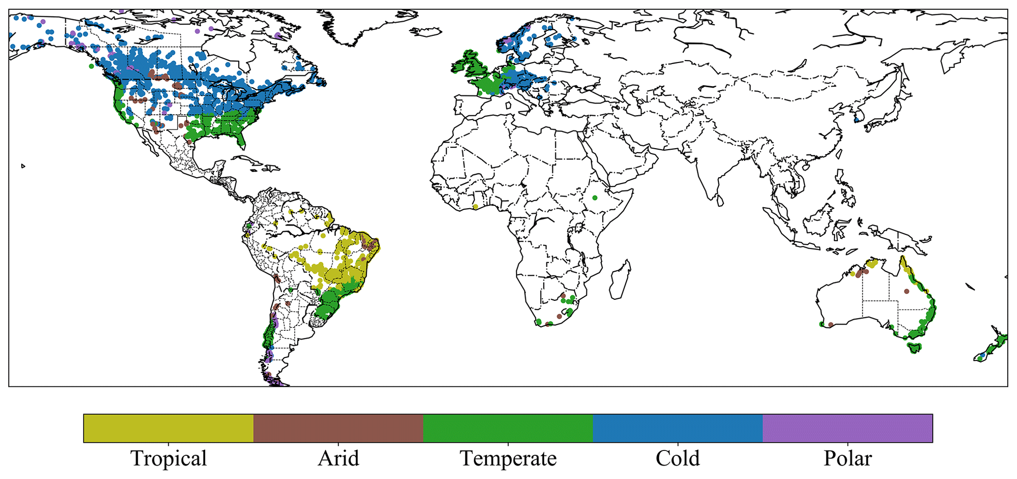
Figure 1Locations and climate groups of the 3753 global basins used in this study, which were originally compiled by Beck et al. (2020a). Plotted in Python using Matplotlib Basemap Toolkit.
2.2 The long short-term memory (LSTM) streamflow model for comparison
Here the LSTM model is used as a purely data-driven benchmark DL model. The LSTM has “cell states” and “gates” to maintain and filter information, as shown in Fig. 2a. The input, forget, and output gates control the flow of information, respectively controlling what to let in, what to forget, and what to output from the system. In this study we use the LSTM streamflow model demonstrated in Feng et al. (2020), which has been successfully applied to simulate streamflow in hundreds of basins across the CONUS. The framework takes meteorological forcings and basin attributes as inputs and generates daily streamflow predictions for each basin at each time step (Fig. 2a). We used mini-batches to train the LSTM model, where each mini-batch was composed of 2-year sequences from 256 randomly selected basins. The first-year sequences are only used for initializing the cell states, so we calculate the batch loss function only on the second-year sequences. The training sequences were also randomly selected from the whole training period, and one epoch was finished when the model had seen all the training data. Note that this sequence length is a subset of, and different concept from, the length of the training period. Sequence length specifically refers to the length of the training instance that comprises a mini-batch, whereas training period refers to the whole period when observations are available for training, from which the mini-batch sequence length is randomly selected. The model was forwarded on each mini-batch iteratively, and its weights were updated using gradient descent after each forwarding. One epoch is regarded as having occurred when the model is iterated over all the training data. We trained the LSTM model for 300 epochs to achieve convergence.
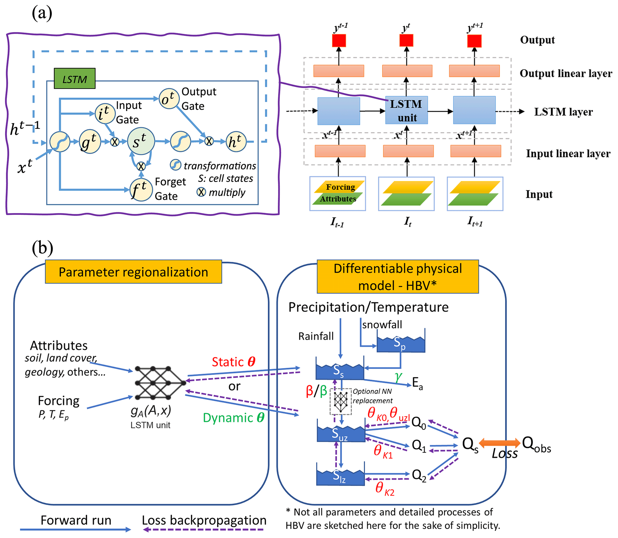
Figure 2Illustrations of two different types of regionalized hydrologic models. (a) Framework of the purely data-driven LSTM streamflow model (adapted from Fig. 2 in Feng et al., 2020) and (b) framework of the differentiable hydrologic model with parameter regionalization, first developed in Feng et al. (2022a), trained on global data (δHBV-globe1.0-hydroDL) (adapted from Fig. 1 in Feng et al., 2022a). Here, the neural network gA is an LSTM unit which is trained by the observed streamflow to produce the static or dynamic physical HBV parameters (θ, β, γ) from basin characteristics.
2.3 The hybrid differentiable hydrologic models
In this work, we used the hybrid differentiable models developed in Feng et al. (2022a) for regionalized modeling in global basins (δHBV-globe1.0-hydroDL). The HBV model used here as the physical backbone is a conceptual hydrologic model with representations of snowpack, soil, and groundwater storages, and it can simulate flux variables such as snow melting, evapotranspiration, and quick and slow outflows (Beck et al., 2020a; Bergström, 1976, 1992; Seibert and Vis, 2012). The differentiable parameter learning (dPL) framework (Tsai et al., 2021) is used to provide parameter regionalization for HBV, as shown by the gA neural network in Fig. 2b. The gA network, which is an LSTM unit here, takes basin attributes and meteorological forcings as inputs, and it outputs static or dynamic physical HBV parameters. The differentiable HBV model then takes these parameters and the meteorological forcings to simulate the hydrologic process and predict daily streamflow discharge along with other key flux variables. The whole framework, including HBV itself, was implemented in a DL platform (PyTorch 1.0.1 was used for the original development, and the model has also shown good compatibility with more recent PyTorch versions; Paszke et al., 2017) supporting automatic differentiation and trained with gradient descent to minimize the difference between the simulated and observed streamflow (the loss function). As in Feng et al. (2022a), we employed the loss function based on root-mean-square error (RMSE) with two weighted parts. The first part calculates RMSE directly on the simulated and observed discharges, while the second part calculates RMSE on the transformed discharge records to improve low flow representations. Note that we do not directly train the HBV parameters; rather, we focus on training the weights of the gA neural network to map the relationship between basin-averaged characteristics and HBV parameters. Differentiable models are also trained in mini-batches that are formed in the same way as for training the LSTM streamflow model. Within one epoch, differentiable models are forwarded and optimized over the randomly formed mini-batches until the iterations have used all the training data points. We train the differentiable models for 50 epochs in total.
As described in Feng et al. (2022a), the differentiable modeling framework enables optional modification of the structures of the original HBV model to enable better performance, and we used two versions of the evolved HBV model in this study. We used 16 parallel subbasin-scale response units, each with a separate set of parameters to describe a fraction of the basin with different hydrologic responses. These components implicitly represent subbasin-scale spatial heterogeneity. The simulated fluxes (e.g., runoff) are the average of all the response units. The parameters of the multiple components are different, and all are produced simultaneously by the same gA network. The first version of our model (referred to as “dPL + evolved HBV”) only has static parameters, which are kept constant during the hydrologic simulation. The second version (referred to as “dPL + evolved HBV with DP) further allows some formerly static parameters of the multi-component model to vary daily with the meteorological forcings. These dynamic parameters (DPs) were also produced by the gA LSTM unit. If we were to apply the dynamic parameterization to all parameters, the model could become overly flexible, potentially leading to overfitting to the training data (which would lead to issues with extrapolation beyond the training data). To reduce the risk of overfitting, we restricted the dynamism to only two empirical parameters: the shape coefficient β in the equation that describes the relationships between soil water and potential runoff and a newly added shape parameter (γ) which is involved in the calculation of evapotranspiration. For more details regarding these differentiable HBV models, please refer to our previous studies (Feng et al., 2022a, 2023).
2.4 Experiments and evaluation metrics
We ran one temporal and two spatial generalization experiments to evaluate the performance of different regionalized models. For the temporal generalization experiment, the models were trained for the period of 2000 to 2016 on all global basins and tested for the period of 1980 to 1997. Basins without discharge records or with less than 5 years' worth of data points in the testing period were excluded from the evaluation. Without spatially holding out any basin during training, this experiment aimed at evaluating the model's generalizability in the time dimension by testing prediction ability on the same basins but in a different time period from the training data. The other two spatial generalization experiments served as the true litmus tests for evaluating the effectiveness of regionalization schemes, i.e., how well the model can be applied to basins that have never been seen during training. The first spatial generalization experiment was a traditional “prediction in ungauged basins” (PUB) problem, where we randomly divided the whole global basin set into 10 folds (groups) and performed cross-validation across these folds to obtain spatial out-of-sample predictions for all basins (training on 9 of the folds, with the 10th fold held out and used for testing, then rotating such that each fold is used for testing once). The second spatial generalization experiment, which we refer to as cross-continent “prediction in ungauged regions” (PUR), was more challenging. In this experiment, we assumed that all the basins in certain continents were ungauged and excluded from the training dataset, trained a regionalized model in other data-rich continents, and then tested the trained model to make predictions in the ungauged continents. With random hold out, an ungauged test basin in the first spatial generalization experiment always has training gauges surrounding it. Therefore, the first PUB experiment can be interpreted as spatial interpolation. The second spatial experiment (cross-continent PUR) holds out all the basins in one continent as testing targets; thus it is the much harder test of spatial extrapolation.
To evaluate the overall performance of the hydrologic models, we used the Kling–Gupta efficiency (KGE) (Gupta et al., 2009; Kling et al., 2012), as compared in Beck et al. (2020a), and the Nash–Sutcliffe efficiency (NSE) (Nash and Sutcliffe, 1970). KGE has three components that account for correlation, mean bias (the ratio of simulated and observed means), and variability bias (the ratio of simulated and observed coefficients of variation), while NSE mainly represents the variance explained by the simulations. Both metrics indicate better performance when their values are closer to the maximum value of 1. We also examined the percent bias of the top 2 % peak flow range (FHV) and bottom 30 % low flow range (FLV) of streamflow predictions to evaluate the model's ability to simulate extreme events (Yilmaz et al., 2008). All the reported performance metrics in this study are from model evaluation on the testing dataset, which is not seen by the model during the training process.
3.1 General patterns over global basins
From the standpoint of daily hydrograph metrics (KGE and NSE), LSTM and the two differentiable models all achieved highly competitive performance for the global basins in the temporal test (trained and tested on the same basins but in different time periods) (Fig. 3). For the global dataset, all three models obtained median KGE values close to or higher than 0.7, but the LSTM model performed the best of the three models here, achieving a median NSE (KGE) value of 0.70 (0.74) for all the evaluated basins. For a subset of 1675 basins with long-term records (at least 15 years' worth of streamflow data available in the training period and 5 years' worth of data available in the testing period, though not necessarily continuous), LSTM even reached a median KGE of 0.78 (see Fig. A1). Both versions of the differentiable models approached the performance level of the LSTM, in agreement with our previous assessment for the CONUS (Feng et al., 2022a). The model with dynamic parameters achieved a median NSE (KGE) of 0.67 (0.69), followed by the model with static parameters, which obtained a median NSE (KGE) of 0.65 (0.68).
The LSTM exhibited advantages for the low flow predictions compared with the differentiable models, as shown by the FLV metric (Fig. 3). However, for the peak flow predictions, the LSTM and differentiable models were quite similar, and they all underestimated the observed peaks (FHV in Fig. 3). The underestimation for peak flows is consistent with what was found in previous studies. For example, all the physical and deep learning models have significant negative peak flow bias when benchmarked in the CONUS dataset (Feng et al., 2020; Kratzert et al., 2019b). We hypothesize that the systematic underestimation of peaks may be partially related to bias in precipitation forcings. MSWEP is based on the ERA5 reanalysis, which is known to underestimate precipitation peaks (Beck et al., 2019). Furthermore, the use of basin-averaged, daily averaged precipitation may further suppress the peaks (Chen et al., 2017). In addition, the errors with peak flow could also be partly due to some numerical and structural issues with the differentiable models, e.g., numerical errors introduced by the explicit and sequential solution scheme of HBV with excessive use of threshold functions that lead to different results when the sequence changes, and structure limitations; e.g., deeper groundwater storage cannot feed back to the upper layers. Given the commonality of this issue, we call for community efforts and collaboration to address this issue.
Both the LSTM model and the differentiable models performed well over diverse landscapes, including North America (especially along the Rocky and Appalachian mountain ranges and the Southeastern Coastal Plains), western Europe, Asia (mostly Japan), the southern part of Brazil, and the northeastern coast of Australia (Fig. 4a and b). There are other regions where none of the three models performed well, such as the longitudinally central part of North America (Great Plains and Interior Lowlands), the southern edge of Chile (with many glaciers), the state of Tasmania in Australia, and the few basins in Africa. These regions, for example, the northern Great Plains and the state of Texas in the CONUS, have always been difficult for all kinds of models, likely due to incorrect basin boundaries, highly localized precipitation, the dry conditions with small runoff amounts, and flash flooding mechanisms (Berghuijs et al., 2014; Driscoll et al., 2002; Feng et al., 2020; Martinez and Gupta, 2010; Newman et al., 2017), which are explored below. Despite some challenges, however, these values currently represent the best metrics reported at the global scale compared to earlier studies (e.g., Alfieri et al., 2020; Beck et al., 2017a, 2020a; Hou et al., 2023), attesting to the great potential of these models as global modeling tools.
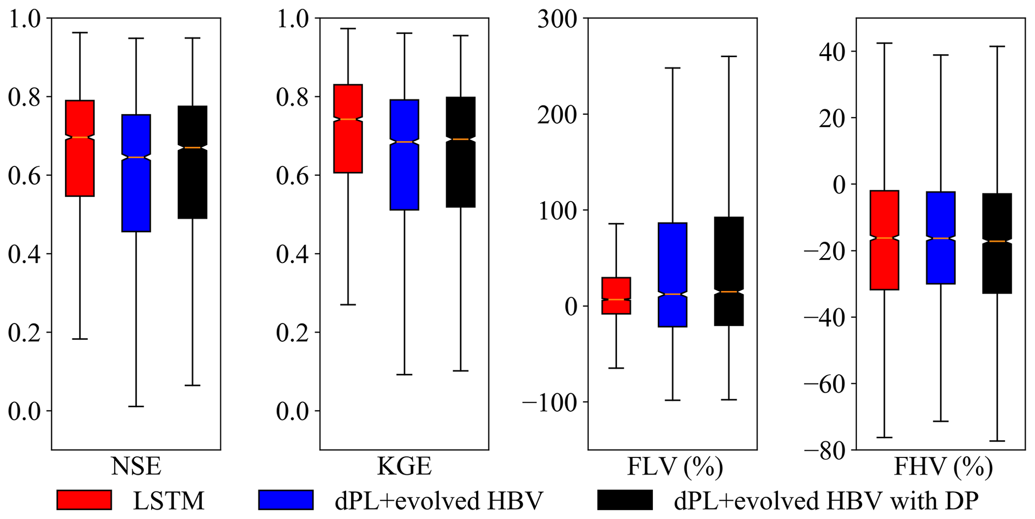
Figure 3Performance comparison between the LSTM and differentiable models on global basins. dPL refers to the differentiable parameter learning framework, “evolved HBV” refers to some modifications to improve the standard HBV model, and “with DP” indicates that some parameters were allowed to be dynamic rather than static. Here, the horizontal line inside the colored box represents the median, while the top and bottom of the colored box indicate the first and third quartiles. The bars extending from the colored boxes indicate the lowest and highest data within 1.5 times the interquartile range from the first and third quantiles. NSE is Nash–Sutcliffe efficiency, KGE is Kling–Gupta efficiency, FLV indicates the model's percent bias on the bottom 30 % low flow range of streamflow, and FHV indicates percent bias on the top 2 % peak flow range of streamflow.
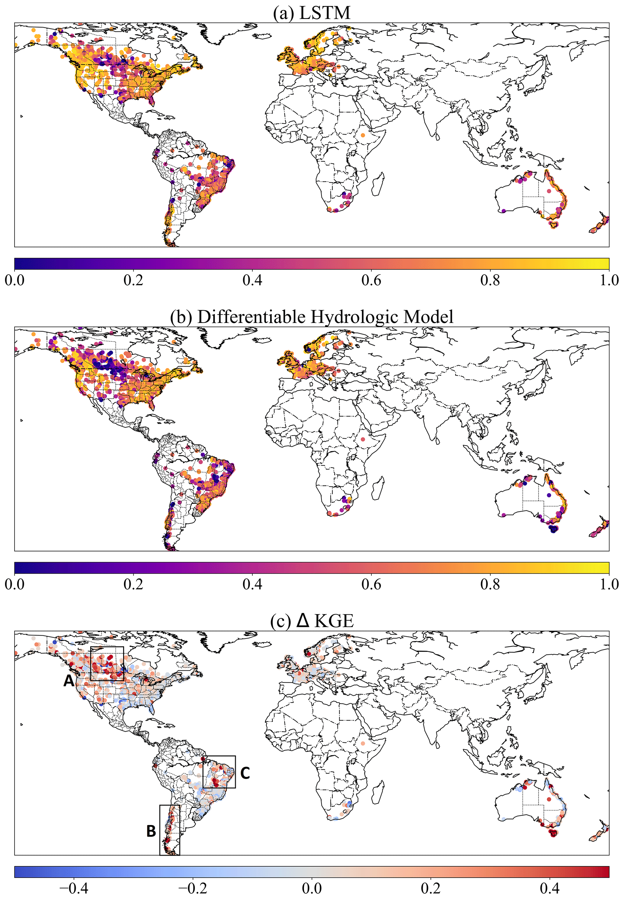
Figure 4The spatial patterns of different model performance and their differences shown by KGE metrics. (a) The LSTM model, (b) the differentiable model with dynamic parameters (dPL + evolved HBV with DP), and (c) the KGE difference between two models (KGE of LSTM − KGE of dPL + evolved HBV with DP). Plotted in Python using Matplotlib Basemap Toolkit.
3.2 Model behaviors and limitations across climate groups and regions
All three models' performances varied significantly across different climate groups of the global basins (Fig. 5), revealing their strengths and limitations. The LSTM model behaved the best in the polar, cold, and temperate groups, while the performance deteriorated in the tropical and arid basins. Similarly to LSTM, differentiable models showed strong performance in temperate and cold groups and worse performance in tropical ones, with the worst performance in arid basins. These clusters of challenging basins can also be identified on the map (Fig. 4a and b). The differentiable model with dynamic parameters performed better than the model with static parameters in all climate groups except the most challenging arid group. Dynamic parameterization with more structural flexibility generally provides stronger modeling ability while also showing a higher risk of overfitting and degraded generalizability in basins which are very difficult to simulate. As we examine how LSTM and differentiable models behave differently, we find that such differences can be attributed to processes missing from the simple process-based backbone model (HBV here), as explained below. Here we use LSTM as an indicator of upper bound; that is, it shows the ideal performance of a model given the available information from forcing and input data. Thus the distance from LSTM indicates either systematic and predictable forcing errors (which can be remediated by LSTM) or structural issues with the differentiable model.
For example, the polar group stands out as a climate type favoring LSTM, while the cold group shows a similar but less pronounced contrast, both of which may be related to HBV's physical deficiencies and forcing issues with snow undercatch. For the polar (cold) groups, LSTM surprisingly had a median KGE of 0.81 (0.78), while the differentiable model only reached 0.62 (0.71). The polar regions include, for example, southern Chile (in region B in Fig. 4c). As glaciers can store water for extended periods of time and are driven mostly by temperature rather than rainfall, it is possible for LSTM to capture the temperature-driven dynamics (Lees et al., 2022), while the original HBV itself does not have a glacial module. HBV does not have the ability to simulate frozen soil, sublimation, or snow cover fractions. Furthermore, as snow gauges at high altitude are known to suffer systematic bias due to undercatch problems (Beck et al., 2020b), LSTM can learn to address such systematic bias, while physical differentiable models cannot due to mass balance. For the cold regions, e.g., high-latitude regions of the North American Great Plains (Region A in Fig. 4c – this also includes the Prairie Pothole Region, or PPR), HBV may suffer from not having descriptions for frozen ground conditions (soil ice) which can influence infiltration and from rainfall underestimation due to undercatch, ice blockage, and other potential reasons (Beck et al., 2020b). In addition, another reason why LSTM and differentiable HBV may have trouble with PPR (but HBV performed especially poorly) is the countless wetlands that store water until full and become connected after snowmelt and large rainfall. HBV does not have modules that can describe such large-scale fill–connect–spill processes (Shaw et al., 2013; Vanderhoof et al., 2017).
A more prominent challenge is the arid regions (middle CONUS, northern Chile, and eastern Brazil in Figs. 1 and 4). This challenge can be attributed to the long duration of low flows which requires long-term memory and to flash floods which result from intense short-duration storms not well represented at the daily scale. Even the LSTM model cannot retain year-long memory and cannot perform well for the baseflow (Feng et al., 2020). Because HBV has a linear reservoir for its slow-flow (lowest) bucket, it can neither generate zero baseflows nor simulate the impact of intense hourly scale rainfall well. These process improvements need to be considered in the future. Another reason for the challenge in arid regions is the lack of reservoir management modules. Arid regions tend to have water management infrastructure that significantly influences streamflow (Veldkamp et al., 2018). Since the HBV model does not have any module representing human impacts on the natural water cycle, the poor performance in middle Brazil in region C may have come from the missing representation of human interferences. There are large populations and intensive agricultural activities in this region which could induce significant impacts on the hydrologic process. Parameter compensations apparently cannot make up for all the missing mechanisms.
The sensitivity of model performance to missing processes in the differentiable models is both good and bad news. It is good news because this means we can identify suitable or insufficient process representations by learning from data. On the other hand, this means more challenges, as we need to increase the process complexity of this model before it can perform well for these basins, unlike the purely data-driven LSTM which is not explicitly concerned with physical processes.
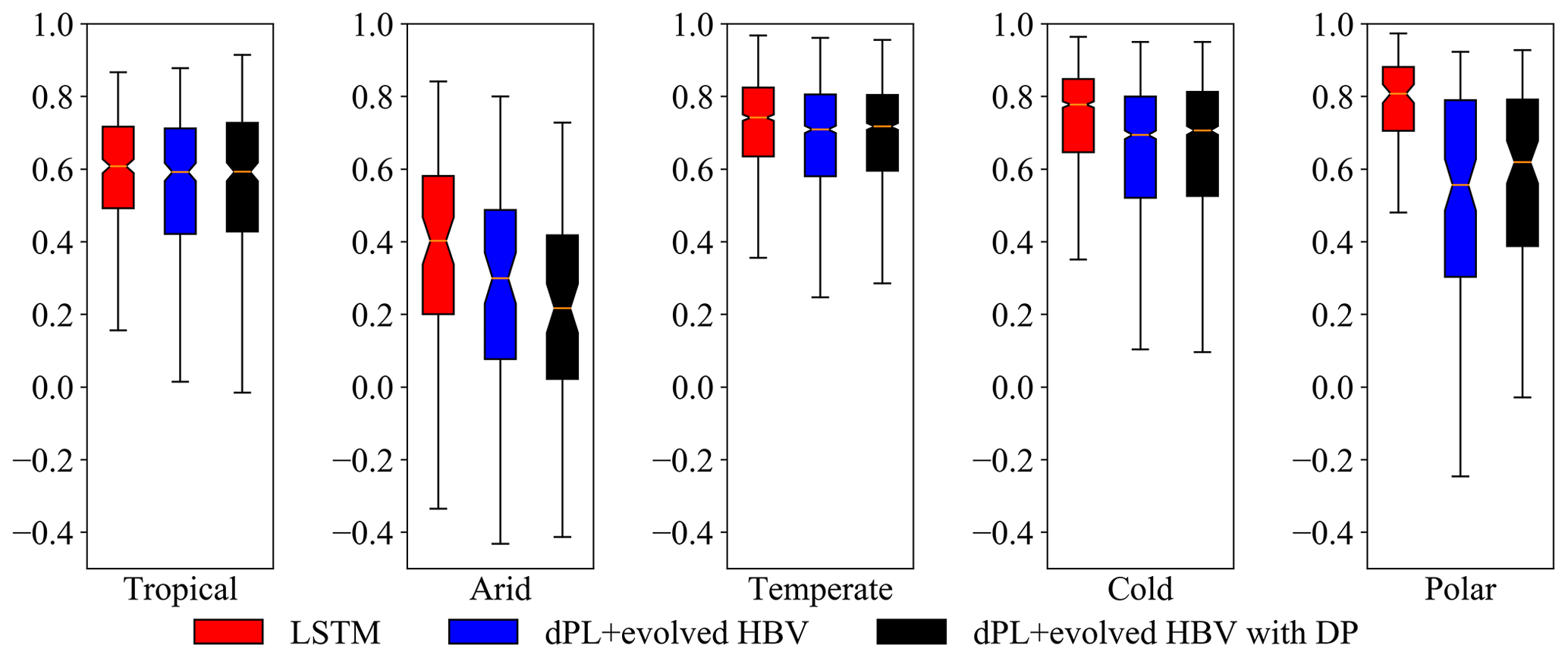
Figure 5The performance comparison (KGE, Kling–Gupta efficiency) of different models for five climate groups. dPL refers to the overall differentiable parameter learning framework, “evolved HBV” refers to some modifications to improve the standard HBV model, and “with DP” indicates that some parameters were allowed to be dynamic rather than static. Here, the horizontal line inside the colored box represents the median, while the top and bottom of the colored box indicate the first and third quartiles. The bars extending from the colored boxes indicate the lowest and highest data within 1.5 times the interquartile range from the first and third quantiles.
3.3 Spatial generalization for prediction in ungauged regions
While LSTM maintains mild advantages over differentiable models in data-dense settings, it was outperformed by differentiable models in a highly data-scarce scenario. As mentioned above, the data-dense setting was tested in the randomized holdout test called prediction in ungauged basins (PUB), while the data-scarce scenario was tested in the regional holdout test, or prediction in ungauged regions (PUR). In the global PUB test, LSTM has a small edge (median KGE of 0.67) over differentiable models (median KGE of 0.64). Both were noticeably higher than the traditional regionalization method using linear transfer functions reported by Beck et al. (2020a) (Beck20, median KGE of 0.46), which already represents the previous state-of-the-art performance of global parameter regionalization. Differentiable modeling does not rely on strong assumptions of the functional form for the parameter transfer function. It leverages the powerful ability of neural networks to represent complicated functions, and it automatically learns robust and generalizable relationships between geographic attributes and physical model parameters from large data. Therefore, we can expect significant performance advantages from differentiable modeling compared to traditional methods relying on linear transfer functions. In the PUR scenario where European basins were held out for testing, differentiable models (median KGE of 0.58) performed significantly better (p-value less than 0.01 using the one-sided Wilcoxon signed-rank test) than LSTM (median KGE of 0.52). In the South American PUR experiment, lower performance was seen for all models, which can be expected considering the prediction difficulties in this region even for the in-sample scenario (Regions B and C in Fig. 4). The median KGE of LSTM is 0.28, while the differentiable model with static parameters achieves a higher median KGE of 0.31 for the PUR scenario. It seemed that the differentiable model with dynamic parameterization was somewhat overfitted in this case, resulting in a median KGE that was lower than the static-parameter differentiable model. We do not have PUR results from traditional models available to compare against, since this is a very challenging issue for traditional regionalization methods to make predictions across continents.
With these results, we show that differentiable models have demonstrated a high simulation capability that cannot be obtained with traditional parameter regionalization approaches, and we also provide a robust extrapolation capability in large data-sparse regions that is stronger than purely data-driven models like LSTM. This conclusion was not only verified in the USA, but it has now also been confirmed in global catchments with generalization tests including prediction in neighboring ungauged basins and cross-continent predictions, each of which has different conditions with respect to data availability and density.
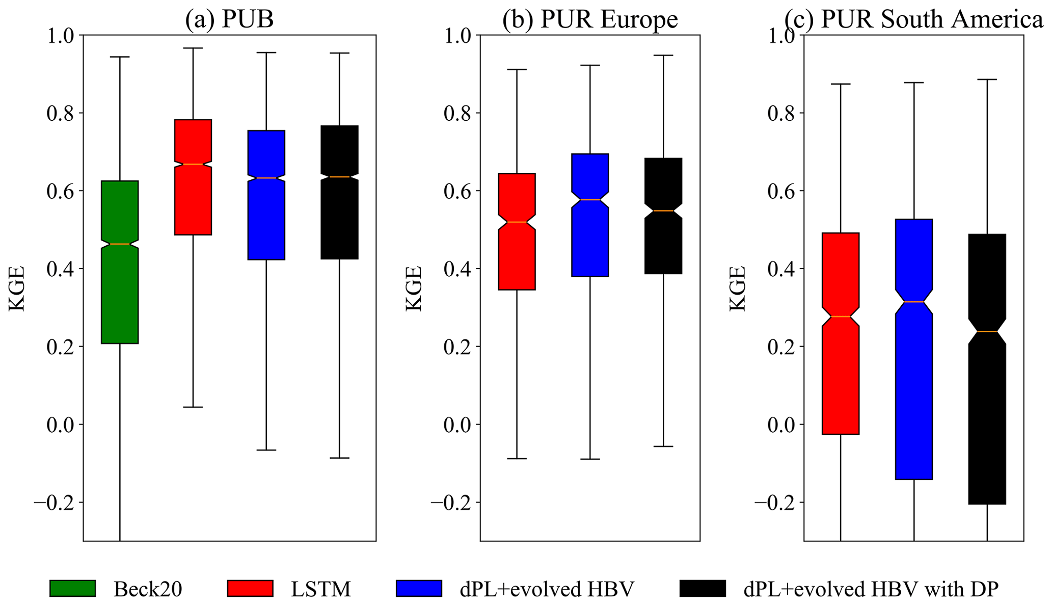
Figure 6The performance comparison (KGE, Kling–Gupta efficiency) of different models for spatial generalization tests. (a) Random hold-out test for prediction in ungauged basins (PUB) and (b, c) holding out all the basins in Europe and South America, respectively, for cross-continent predictions in ungauged regions (PUR). Beck20 refers to a traditional regionalization method using linear transfer functions (Beck et al., 2020a), and LSTM is the purely data-driven long short-term memory network. dPL refers to the differentiable parameter learning framework, “evolved HBV” refers to some modifications to improve the standard HBV model, and “with DP” indicates that some parameters were allowed to be dynamic rather than static. Here, the horizontal line inside the colored box represents the median, while the top and bottom of the colored box indicate the first and third quartiles. The bars extending from the colored boxes indicate the lowest and highest data within 1.5 times the interquartile range from the first and third quantiles.
3.4 Predicting untrained variables
The evapotranspiration (ET) simulations from differentiable models are consistent with independent MODIS satellite estimates of ET in both temporal dynamics and spatial patterns. We did not use any ET observations as training targets to supervise the differentiable models. At the global scale, the mean annual ET comparison shows overall consistency with MODIS, with most basins lying close to the 1:1 line and a correlation of 0.75 for all the basins (Fig. 7a). Spatially, the model was able to represent energy limitations in the cold regions, e.g., high-latitude North America and Europe, and water limitations, e.g., the southwestern US and arid basins of Australia (Fig. 7a and b). The model also represented high ET in basins adjacent to the Amazon forest and those along the US southeastern coast and Australian coast. Temporally, the median correlation of ET time series between simulations and MODIS products achieves 0.82 and 0.89, respectively, for two differentiable models in 3753 basins (Fig. 7c).
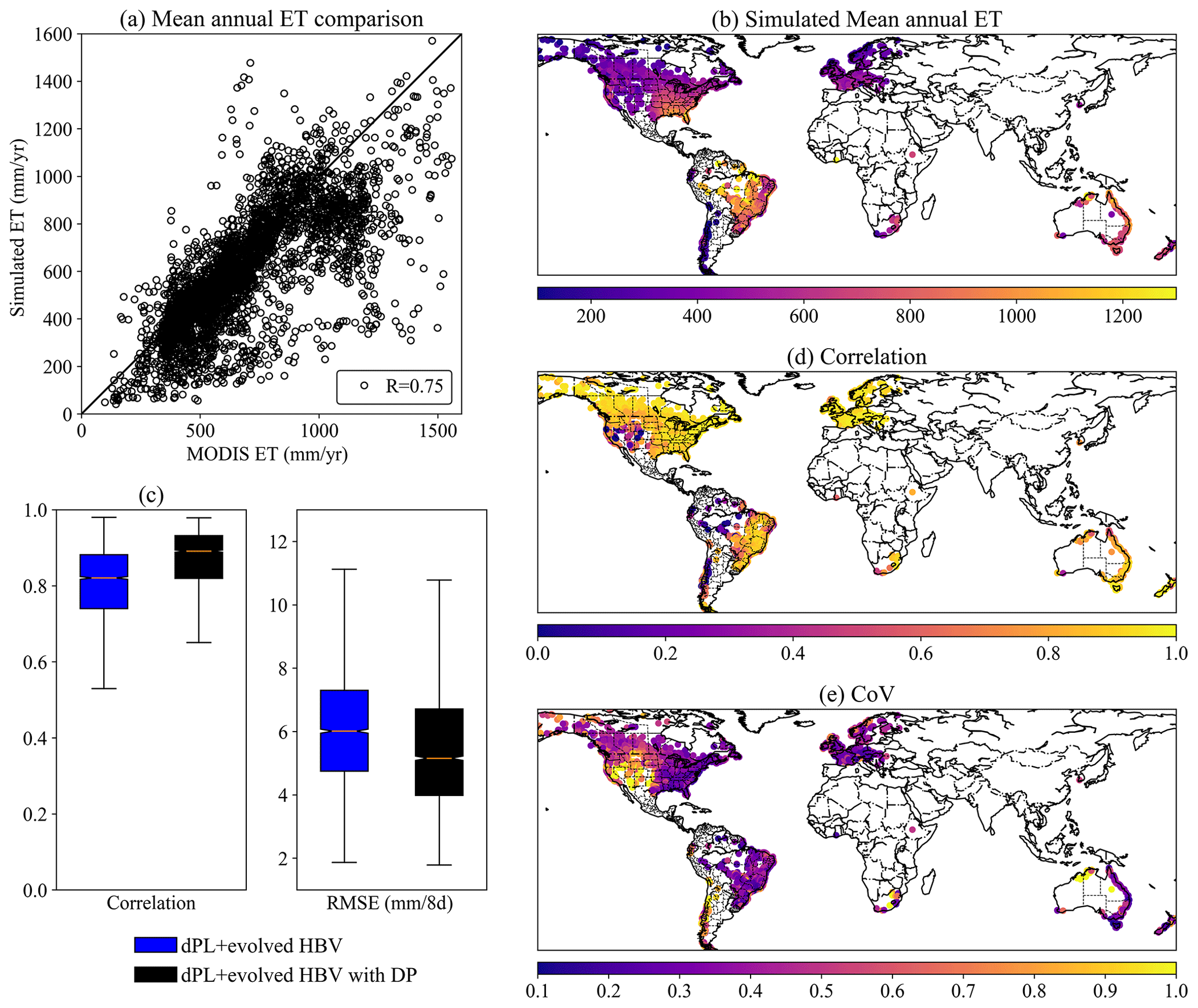
Figure 7The comparison between simulated ET from the differentiable hydrologic models and independent MODIS ET product. (a) Mean annual ET comparison, (b) simulated mean annual ET for global basins, (c) boxplots for the temporal dynamic evaluation by correlation and RMSE, (d) correlation, and (e) coefficient of variation for ET comparison in global basins. Maps plotted in Python using Matplotlib Basemap Toolkit.
The ET simulations show high correlation with MODIS in most North American and European basins (Fig. 7d) in line with good performance on streamflow modeling in these regions. However, the correlation is relatively low in South America, but the coefficient of variation in ET residuals (CoV; the ratio of standard deviation of ET residuals to the annual mean) is also small (Fig. 7e), in part because the ET here is large and less driven by the seasonal energy cycle (Niu et al., 2017). MODIS ET itself is not the ground truth and always has large uncertainties in Amazonia regions due to the cloud coverage and difficulties in observation (Hilker et al., 2015; Xu et al., 2019). Furthermore, the simulations could be negatively influenced by the data quality issues with streamflow records in these regions. Upon examining the records, some stations in South America show unrealistic hydrographs that may indicate data processing errors. To address such issues in the future, more in-depth data screening and correction or constraining the model using datasets other than streamflow, e.g., eddy covariance flux data, should be considered. The CoV is less than 0.3 for most of the world, showing that ET errors are mostly small relative to its annual averages (Fig. 7e). Noticeable exceptions are the US southwest, where ET varies strongly from year to year and is highly dependent on the precipitation, and Chile, where glaciers and deserts are both present, posing challenges to the model. As the present study is basin-focused, we will leave the evaluation of global gridded ET to future work.
3.5 Further discussion
Compared to the LSTM model which only outputs discharge simulations, differentiable models offer a suite of interpretable variables, including ET, soil water, recharge, and baseflow, thus providing a comprehensive description for the hydrologic cycle and far better interpretability. To create a new differentiable model or turn an existing model into a differentiable one, we need to implement the model on a differentiable platform like PyTorch, TensorFlow, or JAX while better enabling model parallelism in order to maximally leverage the computing power of modern graphical processing units (GPUs). If a model contains mostly explicit calculations, automatic differentiation (AD) offered by the above platforms can effortlessly provide gradient calculations, requiring only a syntax-level translation which can nowadays be done easily. Sometimes, a limited number of adjustments are needed to turn non-differentiable operations into equivalent differentiable ones. However, when a model contains iterative solutions to nonlinear systems, large matrix solvers, or constrained optimizations, we can employ the adjoint method (Song et al., 2024b). The adjoint method explicitly defines the gradient calculation method and alters the order of calculations so iteration is avoided during gradient calculations, which can dramatically reduce memory demand and improve efficiency. Another important consideration is the effective use of parallelism and the modern computing infrastructure for AI (i.e., GPUs). In our context, the regionalized parameterization (in this case, training one neural network on a large amount of basins), which is crucial to ensuring the generalizability of the model, requires going through large data in high-throughput parallelism. Embracing parallelism may necessitate some coding adjustments. At this point, several versions of differentiable hydrologic models have been proposed with varying complexities and different handling of parameterization, post-processing (which we did not use in this study, as it can interfere with interpretability of the internal variables, mass balances, and the sensitivity to inputs encoded by the process-based components), and dynamical parameters. Across geoscientific domains, differentiable ecosystem (Aboelyazeed et al., 2023; Zhao et al., 2019), flow and routing (Bindas et al., 2024), water quality (Rahmani et al., 2023), and ice sheet (Bolibar et al., 2023) models have already been demonstrated.
The challenges facing the differentiable models in this study include not only missing processes like reservoir management, ground ice, and glaciers, but also large errors in meteorological forcings and streamflow target data. Substantial bias could exist in precipitation, e.g., due to snow-gauge undercatch (Hou et al., 2023), or in discharge; e.g., streamflow is measured using different approaches which exhibit large variability. As another example, gridded climate forcing data often consistently underestimate the magnitudes of heavy storms (Beck et al., 2017c). While LSTM can easily adapt to systematic bias, such forcing errors put the differentiable models under stress because they cannot reconcile streamflow observations with such forcings given the constraint of mass balances. If our objective is to learn core physics and parameterizations that are reliable despite forcing discrepancies, we can set up forcing data correction layers that can, to some extent, shield the core processes from being influenced by such errors. This will be an important aspect of future work to ensure reliable prediction of future water resources.
The backbone of a differentiable process-based model thus serves as a double-edged sword: when such backbones are essentially correct, they serve as a stabilizing element of the model that mitigates overfitting and improves generalization; when they lack critical processes or when observations have large, unexplained bias, they can drag down model performance and cause compensation between processes. However, the limitations are tractable: future work can gradually incorporate critical processes and include more observations to constrain the learning process, making sure each addition is valuable and accretive. The research community collectively already has substantial experience in evolving Earth system models to include many processes. We expect some processes to be invited back into the differentiable modeling framework. Nevertheless, with differentiable modeling, we now have a new tool that was not previously available: highly flexible deep neural networks that can be placed anywhere in the model, which provide a systematic way of managing model complexity. With their help, such model evolution may take much less time than previously required. However, we still expect the development cycle to take longer than that for purely data-driven models like LSTM, requiring us to view differentiable models as evolving rather than static entities, which need a bit of patience while maturing.
This study builds a benchmark and a basis for model selection and diagnosis for next-generation global hydrologic modeling, which previously did not learn from such large observations. With rigorous tests at the global scale, this study proves that differentiable models are strong candidates as global water models. With powerful spatial generalization ability, they can be applied to characterizing the hydrologic processes in ungauged regions by leveraging learned information on data-rich continents. Differentiable models in this study have already learned the generalizable and robust relationships between geographic attributes and physical model parameters from thousands of global catchments. Therefore, these models can easily be applied in providing seamless global hydrologic modeling with parameters directly generated from worldwide geographic attributes. Future work can use such models and continuously improved observational datasets to produce global hydrologic fluxes while enhancing some process representations in extremely arid, glaciated, or heavily human-influenced basins.
In this work, we used both purely data-driven models and, for the first time, physics-informed differentiable models to simulate rainfall–runoff processes in 3753 global basins. Both types of models achieved highly competitive performance overall for global basins with diverse climate conditions, yielding median KGE values close to or higher than 0.7, which is the state of the art at this large scale. The LSTM still achieved the best performance for the temporal generalization test, but the differentiable HBV models with evolved structure (δHBV-globe1.0-hydroDL) approach the LSTM's performance level. Furthermore, the spatial generalization experiments highlighted the stronger regionalization and extrapolation ability of differentiable models than the traditional modeling approach and LSTM, demonstrating its promise in being applied to data-scarce regions in the world. River routing is not included in this work and will be investigated in the future, possibly also with differentiable approaches (Bindas et al., 2024).
Different models appear to have generally consistent spatial performance patterns with the LSTM model, though obvious distinctions stand out in several local regions. All models achieve good performance in the temperate and cold climate groups, while they all behave unsatisfactorily in the arid group. For the polar group, the differentiable model performed significantly worse than the LSTM. Without any physical constraints, LSTM shows strong power in simulating storage-dominated processes (snow and glacier), while differentiable models are limited by the structure of their physical backbone model, which in this case does not simulate multiyear ice buildup and melt. Another limitation could be soil-sealing processes in extremely arid regions. These regional performance comparisons thus reveal some deficiencies of the physical backbone in δHBV that cannot be mitigated even by advanced neural-network-based parameterization. These insights provide directions for future improvements. Different from purely data-driven models only trained by the target variable, differentiable models constrained by the physical backbone can give accurate simulations for a full set of hydrologic variables in the water cycle, including evapotranspiration, snow water equivalent, water storage, infiltration, and baseflow. As some process limitations are addressed in the future, we believe differentiable models will be strong candidates for next-generation global water models to characterize and predict the hydrologic processes in ungauged regions across the world.
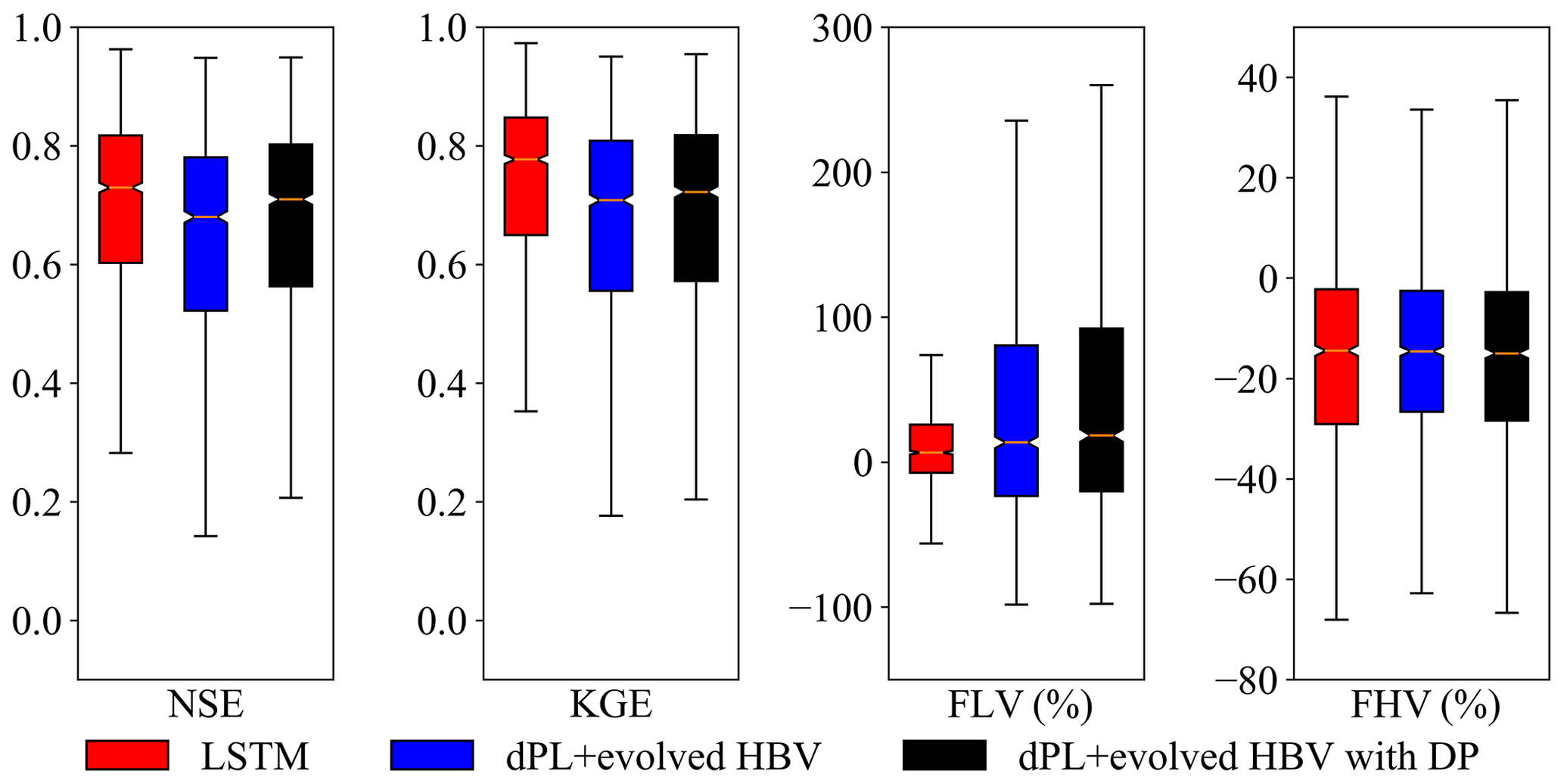
Figure A1Performance comparison of the 1675 subset basins with long-term streamflow records (at least 15 years' worth of streamflow data available in the training period and 5 years' worth of data available in the testing period, not necessarily continuous). Other items are the same as in Fig. 3.
The source codes for the differentiable hydrologic models can be accessed at https://doi.org/10.5281/zenodo.7091334 (Feng et al., 2022b), and this study evaluates these models at global scale. The MOD16A2GF ET product can be downloaded at https://doi.org/10.5067/MODIS/MOD16A2GF.061 (Running et al., 2021). Meteorological forcing datasets MSWEP and MSWX can be downloaded at https://www.gloh2o.org/mswep/ (GloH2O, 2019) and https://www.gloh2o.org/mswx/ (GloH2O, 2022), respectively. The streamflow observations used in this study were initially compiled by Beck et al. (2020a) and can be accessed from the original data sources, including the United States Geological Survey (USGS) National Water Information System (NWIS; https://doi.org/10.5066/F7P55KJN, U.S. Geological Survey, 2024), the Global Runoff Data Centre (GRDC; https://grdc.bafg.de/GRDC/EN/Home/homepage_node.html, GRDC, 2024), the HidroWeb portal of the Brazilian Agência Nacional de Águas (https://www.snirh.gov.br/hidroweb/apresentacao, Brazilian Agência Nacional de Águas, 2024), the European Water Archive (EWA) of EURO-FRIEND-Water (https://www.bafg.de/GRDC/EN/04_spcldtbss/42_EWA/ewa.html; GRDC, 2014), the CCM2-JRC CCM River and Catchment Database (http://data.europa.eu/89h/8c681046-726b-413d-aff8-b1afebd73c0a; de Jager and Vogt, 2003), the Water Survey of Canada (WSC) National Water Data Archive (HYDAT; https://www.canada.ca/en/environment-climate-change/services/water-overview/quantity/monitoring/survey/data-products-services/national-archive-hydat.html, WSC, 2024), the Australian Bureau of Meteorology (BoM; http://www.bom.gov.au/waterdata/, Australia BoM, 2024), and the Chilean Center for Climate and Resilience Research (CR2; https://www.cr2.cl/datos-de-caudales/, Chilean CR2, 2024).
DF and CS conceived this study. DF set up the hydrologic models and ran all the experiments. DF and CS performed the major analysis, with HB, JdB, RKS, YS, YW, and MP contributing substantially to the discussions on the methodology and results. HB provided the benchmark results of the traditional parameter regionalization scheme. JL prepared the ET product for comparison. DF wrote the initial draft, and CS revised the paper. HB, JdB, RKS, YS, YW, and KL substantially edited the paper.
Kathryn Lawson and Chaopeng Shen have financial interests in HydroSapient, Inc., a company which could potentially benefit from the results of this research. This interest has been reviewed by The Pennsylvania State University in accordance with its individual conflict of interest policy, for the purpose of maintaining the objectivity and the integrity of research at The Pennsylvania State University.
Publisher's note: Copernicus Publications remains neutral with regard to jurisdictional claims made in the text, published maps, institutional affiliations, or any other geographical representation in this paper. While Copernicus Publications makes every effort to include appropriate place names, the final responsibility lies with the authors.
We thank the anonymous referees for their comments that helped to improve this paper and the editor for handling the manuscript.
Dapeng Feng was supported by the National Science Foundation Award (award no. EAR-2221880). This work was also partially supported and inspired by the Young Scientists Summer Program (YSSP) of the International Institute for Applied Systems Analysis (IIASA). Jiangtao Liu was supported by Google.org's AI Impacts Challenge (grant no. 1904-57775). Chaopeng Shen and Kathryn Lawson were supported by the Cooperative Institute for Research to Operations in Hydrology (CIROH) (award no. A22-0307-S003). Computation was partially supported by the National Science Foundation Major Research Instrumentation Award (award no. PHY-2018280).
This paper was edited by Lele Shu and reviewed by four anonymous referees.
Aboelyazeed, D., Xu, C., Hoffman, F. M., Liu, J., Jones, A. W., Rackauckas, C., Lawson, K., and Shen, C.: A differentiable, physics-informed ecosystem modeling and learning framework for large-scale inverse problems: demonstration with photosynthesis simulations, Biogeosciences, 20, 2671–2692, https://doi.org/10.5194/bg-20-2671-2023, 2023.
Alfieri, L., Lorini, V., Hirpa, F. A., Harrigan, S., Zsoter, E., Prudhomme, C., and Salamon, P.: A global streamflow reanalysis for 1980–2018, J. Hydrol. X, 6, 100049, https://doi.org/10.1016/j.hydroa.2019.100049, 2020.
Australia BoM: Water Data Online: Water Information, Australia Bureau of Meteorology (BoM) [data set], http://www.bom.gov.au/waterdata/ (last access: 1 May 2022), 2024.
Beck, H. E., van Dijk, A. I. J. M., de Roo, A., Dutra, E., Fink, G., Orth, R., and Schellekens, J.: Global evaluation of runoff from 10 state-of-the-art hydrological models, Hydrol. Earth Syst. Sci., 21, 2881–2903, https://doi.org/10.5194/hess-21-2881-2017, 2017a.
Beck, H. E., van Dijk, A. I. J. M., Levizzani, V., Schellekens, J., Miralles, D. G., Martens, B., and de Roo, A.: MSWEP: 3-hourly 0.25° global gridded precipitation (1979–2015) by merging gauge, satellite, and reanalysis data, Hydrol. Earth Syst. Sci., 21, 589–615, https://doi.org/10.5194/hess-21-589-2017, 2017b.
Beck, H. E., Vergopolan, N., Pan, M., Levizzani, V., van Dijk, A. I. J. M., Weedon, G. P., Brocca, L., Pappenberger, F., Huffman, G. J., and Wood, E. F.: Global-scale evaluation of 22 precipitation datasets using gauge observations and hydrological modeling, Hydrol. Earth Syst. Sci., 21, 6201–6217, https://doi.org/10.5194/hess-21-6201-2017, 2017c.
Beck, H. E., Wood, E. F., Pan, M., Fisher, C. K., Miralles, D. G., Dijk, A. I. J. M. van, McVicar, T. R., and Adler, R. F.: MSWEP V2 Global 3-Hourly 0.1° Precipitation: Methodology and Quantitative Assessment, B. Am. Meteorol. Soc., 100, 473–500, https://doi.org/10.1175/BAMS-D-17-0138.1, 2019.
Beck, H. E., Pan, M., Lin, P., Seibert, J., van Dijk, A. I. J. M., and Wood, E. F.: Global fully distributed parameter regionalization based on observed streamflow from 4,229 headwater catchments, J. Geophys. Res.-Atmos., 125, e2019JD031485, https://doi.org/10.1029/2019JD031485, 2020a.
Beck, H. E., Wood, E. F., McVicar, T. R., Zambrano-Bigiarini, M., Alvarez-Garreton, C., Baez-Villanueva, O. M., Sheffield, J., and Karger, D. N.: Bias correction of global high-resolution precipitation climatologies using streamflow observations from 9372 catchments, J. Climate, 33, 1299–1315, https://doi.org/10.1175/JCLI-D-19-0332.1, 2020b.
Beck, H. E., van Dijk, A. I. J. M., Larraondo, P. R., McVicar, T. R., Pan, M., Dutra, E., and Miralles, D. G.: MSWX: Global 3-hourly 0.1° bias-corrected meteorological data including near real-time updates and forecast ensembles, B. Am. Meteorol. Soc., 103, E710–E732, https://doi.org/10.1175/BAMS-D-21-0145.1, 2022.
Berghuijs, W. R., Sivapalan, M., Woods, R. A., and Savenije, H. H. G.: Patterns of similarity of seasonal water balances: A window into streamflow variability over a range of time scales, Water Resour. Res., 50, 5638–5661, https://doi.org/10.1002/2014WR015692, 2014.
Bergström, S.: Development and application of a conceptual runoff model for Scandinavian catchments, PhD Thesis, Swedish Meteorological and Hydrological Institute (SMHI), Norköping, Sweden, 1976.
Bergström, S.: The HBV model – its structure and applications, Swedish Meteorological and Hydrological Institute (SMHI), Norrköping, Sweden, 1992.
Bindas, T., Tsai, W.-P., Liu, J., Rahmani, F., Feng, D., Bian, Y., Lawson, K., and Shen, C.: Improving river routing using a differentiable Muskingum-Cunge model and physics-informed machine learning, Water Resour. Res., 60, e2023WR035337, https://doi.org/10.1029/2023WR035337, 2024.
Bolibar, J., Sapienza, F., Maussion, F., Lguensat, R., Wouters, B., and Pérez, F.: Universal differential equations for glacier ice flow modelling, Geosci. Model Dev., 16, 6671–6687, https://doi.org/10.5194/gmd-16-6671-2023, 2023.
Brazilian Agência Nacional de Águas: HidroWeb Portal, Brazilian Agência Nacional de Águas [data set], https://www.snirh.gov.br/hidroweb/apresentacao (last access: 1 May 2022), 2024.
Burek, P., Satoh, Y., Kahil, T., Tang, T., Greve, P., Smilovic, M., Guillaumot, L., Zhao, F., and Wada, Y.: Development of the Community Water Model (CWatM v1.04) – a high-resolution hydrological model for global and regional assessment of integrated water resources management, Geosci. Model Dev., 13, 3267–3298, https://doi.org/10.5194/gmd-13-3267-2020, 2020.
Chen, B., Krajewski, W. F., Liu, F., Fang, W., and Xu, Z.: Estimating instantaneous peak flow from mean daily flow, Hydrol. Res., 48, 1474–1488, https://doi.org/10.2166/nh.2017.200, 2017.
Chilean CR2: Flow Data, Chilean Center for Climate and Resilience Research (CR2) [data set], https://www.cr2.cl/datos-de-caudales/ (last access: 1 May 2022), 2024.
Cui, G., Anderson, M., and Bales, R.: Mapping of snow water equivalent by a deep-learning model assimilating snow observations, J. Hydrol., 616, 128835, https://doi.org/10.1016/j.jhydrol.2022.128835, 2023.
de Jager, A. and Vogt, J.: Rivers and Catchments of Europe – Catchment Characterisation Model (CCM), European Commission, Joint Research Centre (JRC) [data set], http://data.europa.eu/89h/8c681046-726b-413d-aff8-b1afebd73c0a (last access: 1 May 2022), 2003.
Driscoll, D. G., Carter, J. M., Williamson, J. E., and Putnam, L. D.: Hydrology of the Black Hills Area, South Dakota (Water Resources Investigation Report 02–4094), US Geological Survey, http://pubs.usgs.gov/wri/wri024094/ (last access: 1 September 2023), 2002.
Fang, K. and Shen, C.: Near-real-time forecast of satellite-based soil moisture using long short-term memory with an adaptive data integration kernel, J. Hydrometeor., 21, 399–413, https://doi.org/10.1175/jhm-d-19-0169.1, 2020.
Fang, K., Shen, C., Kifer, D., and Yang, X.: Prolongation of SMAP to spatiotemporally seamless coverage of continental U.S. using a deep learning neural network, Geophys. Res. Lett., 44, 11030–11039, https://doi.org/10.1002/2017gl075619, 2017.
Fang, K., Pan, M., and Shen, C.: The value of SMAP for long-term soil moisture estimation with the help of deep learning, IEEE T. Geosci. Remote, 57, 2221–2233, https://doi.org/10.1109/TGRS.2018.2872131, 2019.
Fang, K., Kifer, D., Lawson, K., Feng, D., and Shen, C.: The data synergy effects of time-series deep learning models in hydrology, Water Resour. Res., 58, e2021WR029583, https://doi.org/10.1029/2021WR029583, 2022.
Feng, D., Fang, K., and Shen, C.: Enhancing streamflow forecast and extracting insights using long-short term memory networks with data integration at continental scales, Water Resour. Res., 56, e2019WR026793, https://doi.org/10.1029/2019WR026793, 2020.
Feng, D., Lawson, K., and Shen, C.: Mitigating prediction error of deep learning streamflow models in large data-sparse regions with ensemble modeling and soft data, Geophys. Res. Lett., 48, e2021GL092999, https://doi.org/10.1029/2021GL092999, 2021.
Feng, D., Liu, J., Lawson, K., and Shen, C.: Differentiable, learnable, regionalized process-based models with multiphysical outputs can approach state-of-the-art hydrologic prediction accuracy, Water Resour. Res., 58, e2022WR032404, https://doi.org/10.1029/2022WR032404, 2022a.
Feng, D., Shen, C., Liu, J., Lawson, K., and Beck, H.: differentiable parameter learning (dPL) + HBV hydrologic model, Zenodo [code], https://doi.org/10.5281/zenodo.7091334, 2022b.
Feng, D., Beck, H., Lawson, K., and Shen, C.: The suitability of differentiable, physics-informed machine learning hydrologic models for ungauged regions and climate change impact assessment, Hydrol. Earth Syst. Sci., 27, 2357–2373, https://doi.org/10.5194/hess-27-2357-2023, 2023.
GloH2O: MSWEP, GloH2O [data set], https://www.gloh2o.org/mswep/ (last access: 1 May 2022), 2019.
GloH2O: MSWX, GloH2O [data set], https://www.gloh2o.org/mswx/ (last access: 1 May 2022), 20222.
GRDC: European Water Archive (EWA) of EURO-FRIEND-Water, GRDC [data set], https://grdc.bafg.de/GRDC/EN/04_spcldtbss/42_EWA/ewa.html (last access: 1 May 2022), 2014.
GRDC: River Discharge Data, Global Runoff Data Center (GRDC) [data set], https://grdc.bafg.de/GRDC/EN/Home/homepage_node.html (last access: 1 May 2022), 2024.
Gupta, H. V., Kling, H., Yilmaz, K. K., and Martinez, G. F.: Decomposition of the mean squared error and NSE performance criteria: Implications for improving hydrological modelling, J. Hydrol., 377, 80–91, https://doi.org/10.1016/j.jhydrol.2009.08.003, 2009.
Hagemann, S., Chen, C., Clark, D. B., Folwell, S., Gosling, S. N., Haddeland, I., Hanasaki, N., Heinke, J., Ludwig, F., Voss, F., and Wiltshire, A. J.: Climate change impact on available water resources obtained using multiple global climate and hydrology models, Earth Syst. Dynam., 4, 129–144, https://doi.org/10.5194/esd-4-129-2013, 2013.
Hansen, L. D., Stokholm-Bjerregaard, M., and Durdevic, P.: Modeling phosphorous dynamics in a wastewater treatment process using Bayesian optimized LSTM, Comput. Chem. Eng., 160, 107738, https://doi.org/10.1016/j.compchemeng.2022.107738, 2022.
Hargreaves, G. H.: Defining and using reference evapotranspiration, J. Irrig. Drain. Eng., 120, 1132–1139, https://doi.org/10.1061/(ASCE)0733-9437(1994)120:6(1132), 1994.
Hattermann, F. F., Krysanova, V., Gosling, S. N., Dankers, R., Daggupati, P., Donnelly, C., Flörke, M., Huang, S., Motovilov, Y., Buda, S., Yang, T., Müller, C., Leng, G., Tang, Q., Portmann, F. T., Hagemann, S., Gerten, D., Wada, Y., Masaki, Y., Alemayehu, T., Satoh, Y., and Samaniego, L.: Cross-scale intercomparison of climate change impacts simulated by regional and global hydrological models in eleven large river basins, Clim. Change, 141, 561–576, https://doi.org/10.1007/s10584-016-1829-4, 2017.
Hilker, T., Lyapustin, A. I., Hall, F. G., Myneni, R., Knyazikhin, Y., Wang, Y., Tucker, C. J., and Sellers, P. J.: On the measurability of change in Amazon vegetation from MODIS, Remote Sens. Environ., 166, 233–242, https://doi.org/10.1016/j.rse.2015.05.020, 2015.
Hochreiter, S. and Schmidhuber, J.: Long Short-Term Memory, Neural Computation, 9, 1735–1780, https://doi.org/10.1162/neco.1997.9.8.1735, 1997.
Höge, M., Scheidegger, A., Baity-Jesi, M., Albert, C., and Fenicia, F.: Improving hydrologic models for predictions and process understanding using neural ODEs, Hydrol. Earth Syst. Sci., 26, 5085–5102, https://doi.org/10.5194/hess-26-5085-2022, 2022.
Hou, Y., Guo, H., Yang, Y., and Liu, W.: Global Evaluation of Runoff Simulation From Climate, Hydrological and Land Surface Models, Water Resour. Res., 59, e2021WR031817, https://doi.org/10.1029/2021WR031817, 2023.
Jayakrishnan, R., Srinivasan, R., Santhi, C., and Arnold, J. G.: Advances in the application of the SWAT model for water resources management, Hydrol. Process., 19, 749–762, https://doi.org/10.1002/hyp.5624, 2005.
Jiang, S., Zheng, Y., and Solomatine, D.: Improving AI system awareness of geoscience knowledge: Symbiotic integration of physical approaches and deep learning, Geophys. Res. Lett., 47, e2020GL088229, https://doi.org/10.1029/2020GL088229, 2020.
Kling, H., Fuchs, M., and Paulin, M.: Runoff conditions in the upper Danube basin under an ensemble of climate change scenarios, J. Hydrol., 424–425, 264–277, https://doi.org/10.1016/j.jhydrol.2012.01.011, 2012.
Konapala, G., Kao, S.-C., Painter, S. L., and Lu, D.: Machine learning assisted hybrid models can improve streamflow simulation in diverse catchments across the conterminous US, Environ. Res. Lett., 15, 104022, https://doi.org/10.1088/1748-9326/aba927, 2020.
Kraft, B., Jung, M., Körner, M., Koirala, S., and Reichstein, M.: Towards hybrid modeling of the global hydrological cycle, Hydrol. Earth Syst. Sci., 26, 1579–1614, https://doi.org/10.5194/hess-26-1579-2022, 2022.
Kratzert, F., Klotz, D., Herrnegger, M., Sampson, A. K., Hochreiter, S., and Nearing, G. S.: Toward improved predictions in ungauged basins: Exploiting the power of machine learning, Water Resour. Res., 55, 11344–11354, https://doi.org/10/gg4ck8, 2019a.
Kratzert, F., Klotz, D., Shalev, G., Klambauer, G., Hochreiter, S., and Nearing, G.: Towards learning universal, regional, and local hydrological behaviors via machine learning applied to large-sample datasets, Hydrol. Earth Syst. Sci., 23, 5089–5110, https://doi.org/10.5194/hess-23-5089-2019, 2019b.
Lees, T., Buechel, M., Anderson, B., Slater, L., Reece, S., Coxon, G., and Dadson, S. J.: Benchmarking data-driven rainfall–runoff models in Great Britain: a comparison of long short-term memory (LSTM)-based models with four lumped conceptual models, Hydrol. Earth Syst. Sci., 25, 5517–5534, https://doi.org/10.5194/hess-25-5517-2021, 2021.
Lees, T., Reece, S., Kratzert, F., Klotz, D., Gauch, M., De Bruijn, J., Kumar Sahu, R., Greve, P., Slater, L., and Dadson, S. J.: Hydrological concept formation inside long short-term memory (LSTM) networks, Hydrol. Earth Syst. Sci., 26, 3079–3101, https://doi.org/10.5194/hess-26-3079-2022, 2022.
Liu, J., Bian, Y., Lawson, K., and Shen, C.: Probing the limit of hydrologic predictability with the Transformer network, J. Hydrol., 637, 131389, https://doi.org/10.1016/j.jhydrol.2024.131389, 2024.
Mai, J., Shen, H., Tolson, B. A., Gaborit, É., Arsenault, R., Craig, J. R., Fortin, V., Fry, L. M., Gauch, M., Klotz, D., Kratzert, F., O'Brien, N., Princz, D. G., Rasiya Koya, S., Roy, T., Seglenieks, F., Shrestha, N. K., Temgoua, A. G. T., Vionnet, V., and Waddell, J. W.: The Great Lakes Runoff Intercomparison Project Phase 4: the Great Lakes (GRIP-GL), Hydrol. Earth Syst. Sci., 26, 3537–3572, https://doi.org/10.5194/hess-26-3537-2022, 2022.
Maidment, D. R.: Conceptual Framework for the National Flood Interoperability Experiment, JAWRA J. Am. Water Resour. A., 53, 245–257, https://doi.org/10/f97pz3, 2017.
Martinez, G. F. and Gupta, H. V.: Toward improved identification of hydrological models: A diagnostic evaluation of the “abcd” monthly water balance model for the conterminous United States, Water Resour. Res., 46, W08507, https://doi.org/10.1029/2009WR008294, 2010.
Mizukami, N., Clark, M. P., Newman, A. J., Wood, A. W., Gutmann, E. D., Nijssen, B., Rakovec, O., and Samaniego, L.: Towards seamless large-domain parameter estimation for hydrologic models, Water Resour. Res., 53, 8020–8040, https://doi.org/10/gcg2dm, 2017.
Müller Schmied, H., Eisner, S., Franz, D., Wattenbach, M., Portmann, F. T., Flörke, M., and Döll, P.: Sensitivity of simulated global-scale freshwater fluxes and storages to input data, hydrological model structure, human water use and calibration, Hydrol. Earth Syst. Sci., 18, 3511–3538, https://doi.org/10.5194/hess-18-3511-2014, 2014.
Nash, J. E. and Sutcliffe, J. V.: River flow forecasting through conceptual models part I – A discussion of principles, J. Hydrol., 10, 282–290, https://doi.org/10.1016/0022-1694(70)90255-6, 1970.
Newman, A. J., Mizukami, N., Clark, M. P., Wood, A. W., Nijssen, B., Nearing, G., Newman, A. J., Mizukami, N., Clark, M. P., Wood, A. W., Nijssen, B., and Nearing, G.: Benchmarking of a Physically Based Hydrologic Model, J. Hydrometeorol., 18, 2215–2225, https://doi.org/10/gbwr9s, 2017.
Niu, J., Shen, C., Chambers, J., Melack, J. M., and Riley, W. J.: Interannual variation in hydrologic budgets in an Amazonian watershed with a coupled subsurface – land surface process model, J. Hydrometeorol., 18, 2597–2617, https://doi.org/10.1175/JHM-D-17-0108.1, 2017.
Paszke, A., Gross, S., Chintala, S., Chanan, G., Yang, E., DeVito, Z., Lin, Z., Desmaison, A., Antiga, L., and Lerer, A.: Automatic differentiation in PyTorch, in: 31st Conference on Neural Information Processing Systems (NIPS 2017), 4–9 December 2017, Long Beach, CA, 2017.
Rahmani, F., Lawson, K., Ouyang, W., Appling, A., Oliver, S., and Shen, C.: Exploring the exceptional performance of a deep learning stream temperature model and the value of streamflow data, Environ. Res. Lett., 16, 024025, https://doi.org/10.1088/1748-9326/abd501, 2021.
Rahmani, F., Appling, A., Feng, D., Lawson, K., and Shen, C.: Identifying structural priors in a hybrid differentiable model for stream water temperature modeling, Water Resour. Res., 59, e2023WR034420, https://doi.org/10.1029/2023WR034420, 2023.
Reichert, P., Ma, K., Höge, M., Fenicia, F., Baity-Jesi, M., Feng, D., and Shen, C.: Metamorphic testing of machine learning and conceptual hydrologic models, Hydrol. Earth Syst. Sci., 28, 2505–2529, https://doi.org/10.5194/hess-28-2505-2024, 2024.
Running, S., Mu, Q., Zhao, M., and Moreno, A.: MODIS/Terra Net Evapotranspiration Gap-Filled 8-Day L4 Global 500m SIN Grid V061, NASA EOSDIS Land Processes Distributed Active Archive Center [data set], https://doi.org/10.5067/MODIS/MOD16A2GF.061, 2021.
Saha, G., Rahmani, F., Shen, C., Li, L., and Cibin, R.: A deep learning-based novel approach to generate continuous daily stream nitrate concentration for nitrate data-sparse watersheds, Sci. Total Environ., 878, 162930, https://doi.org/10.1016/j.scitotenv.2023.162930, 2023.
Seibert, J. and Vis, M. J. P.: Teaching hydrological modeling with a user-friendly catchment-runoff-model software package, Hydrol. Earth Syst. Sci., 16, 3315–3325, https://doi.org/10.5194/hess-16-3315-2012, 2012.
Shaw, D. A., Pietroniro, A., and Martz, L. w.: Topographic analysis for the prairie pothole region of Western Canada, Hydrol. Process., 27, 3105–3114, https://doi.org/10.1002/hyp.9409, 2013.
Shen, C.: A transdisciplinary review of deep learning research and its relevance for water resources scientists, Water Resour. Res., 54, 8558–8593, https://doi.org/10.1029/2018wr022643, 2018.
Shen, C., Appling, A. P., Gentine, P., Bandai, T., Gupta, H., Tartakovsky, A., Baity-Jesi, M., Fenicia, F., Kifer, D., Li, L., Liu, X., Ren, W., Zheng, Y., Harman, C. J., Clark, M., Farthing, M., Feng, D., Kumar, P., Aboelyazeed, D., Rahmani, F., Song, Y., Beck, H. E., Bindas, T., Dwivedi, D., Fang, K., Höge, M., Rackauckas, C., Mohanty, B., Roy, T., Xu, C., and Lawson, K.: Differentiable modelling to unify machine learning and physical models for geosciences, Nat. Rev. Earth Environ., 4, 552–567, https://doi.org/10.1038/s43017-023-00450-9, 2023.
Song, Y., Chaemchuen, P., Rahmani, F., Zhi, W., Li, L., Liu, X., Boyer, E., Bindas, T., Lawson, K., and Shen, C.: Deep learning insights into suspended sediment concentrations across the conterminous United States: Strengths and limitations, J. Hydrol., 639, 131573, https://doi.org/10.1016/j.jhydrol.2024.131573, 2024a.
Song, Y., Knoben, W. J. M., Clark, M. P., Feng, D., Lawson, K., Sawadekar, K., and Shen, C.: When ancient numerical demons meet physics-informed machine learning: adjoint-based gradients for implicit differentiable modeling, Hydrol. Earth Syst. Sci., 28, 3051–3077, https://doi.org/10.5194/hess-28-3051-2024, 2024b.
Song, Y., Tsai, W.-P., Gluck, J., Rhoades, A., Zarzycki, C., McCrary, R., Lawson, K., and Shen, C.: LSTM-based data integration to improve snow water equivalent prediction and diagnose error sources, J. Hydrometeorol., 25, 223–237, https://doi.org/10.1175/JHM-D-22-0220.1, 2024c.
Tsai, W.-P., Feng, D., Pan, M., Beck, H., Lawson, K., Yang, Y., Liu, J., and Shen, C.: From calibration to parameter learning: Harnessing the scaling effects of big data in geoscientific modeling, Nat. Commun., 12, 5988, https://doi.org/10.1038/s41467-021-26107-z, 2021.
U.S. Geological Survey: USGS Water Data for the Nation, U.S. Geological Survey National Water Information System database [data set], https://doi.org/10.5066/F7P55KJN, 2024.
Vanderhoof, M. K., Christensen, J. R., and Alexander, L. C.: Patterns and drivers for wetland connections in the Prairie Pothole Region, United States, Wetlands Ecol. Manage., 25, 275–297, https://doi.org/10.1007/s11273-016-9516-9, 2017.
Vaswani, A., Shazeer, N., Parmar, N., Uszkoreit, J., Jones, L., Gomez, A. N., Kaiser, Ł., and Polosukhin, I.: Attention is All you Need. Advances in Neural Information Processing Systems, 30, edited by: Guyon, I., Von Luxburg, U., Bengio, S., Wallach, H., Fergus, R., Vishwanathan, S., and Garnett, R., ISBN 9781510860964, https://papers.nips.cc/paper_files/paper/2017/hash/3f5ee243547dee91fbd053c1c4a845aa-Abstract.html (last access: 1 September 2023), 2017.
Veldkamp, T. I. E., Zhao, F., Ward, P. J., Moel, H. de, Aerts, J. C. J. H., Schmied, H. M., Portmann, F. T., Masaki, Y., Pokhrel, Y., Liu, X., Satoh, Y., Gerten, D., Gosling, S. N., Zaherpour, J., and Wada, Y.: Human impact parameterizations in global hydrological models improve estimates of monthly discharges and hydrological extremes: a multi-model validation study, Environ. Res. Lett., 13, 055008, https://doi.org/10.1088/1748-9326/aab96f, 2018.
Werth, S. and Güntner, A.: Calibration analysis for water storage variability of the global hydrological model WGHM, Hydrol. Earth Syst. Sci., 14, 59–78, https://doi.org/10.5194/hess-14-59-2010, 2010.
WSC: National Water Data Archive: HYDAT, Water Survey of Canada (WSC), https://www.canada.ca/en/environment-climate-change/services/water-overview/quantity/monitoring/survey/data-products-services/national-archive-hydat.html (1 May 2022), 2024.
Wunsch, A., Liesch, T., and Broda, S.: Groundwater level forecasting with artificial neural networks: a comparison of long short-term memory (LSTM), convolutional neural networks (CNNs), and non-linear autoregressive networks with exogenous input (NARX), Hydrol. Earth Syst. Sci., 25, 1671–1687, https://doi.org/10.5194/hess-25-1671-2021, 2021.
Xu, D., Agee, E., Wang, J., and Ivanov, V. Y.: Estimation of Evapotranspiration of Amazon Rainforest Using the Maximum Entropy Production Method, Geophys. Res. Lett., 46, 1402–1412, https://doi.org/10.1029/2018GL080907, 2019.
Yilmaz, K. K., Gupta, H. V., and Wagener, T.: A process-based diagnostic approach to model evaluation: Application to the NWS distributed hydrologic model, Water Resour. Res., 44, W09417, https://doi.org/10.1029/2007WR006716, 2008.
Zaherpour, J., Gosling, S. N., Mount, N., Schmied, H. M., Veldkamp, T. I. E., Dankers, R., Eisner, S., Gerten, D., Gudmundsson, L., Haddeland, I., Hanasaki, N., Kim, H., Leng, G., Liu, J., Masaki, Y., Oki, T., Pokhrel, Y., Satoh, Y., Schewe, J., and Wada, Y.: Worldwide evaluation of mean and extreme runoff from six global-scale hydrological models that account for human impacts, Environ. Res. Lett., 13, 065015, https://doi.org/10.1088/1748-9326/aac547, 2018.
Zhao, W. L., Gentine, P., Reichstein, M., Zhang, Y., Zhou, S., Wen, Y., Lin, C., Li, X., and Qiu, G. Y.: Physics-constrained machine learning of evapotranspiration, Geophys. Res. Lett., 46, 14496–14507, https://doi.org/10.1029/2019gl085291, 2019.
Zhi, W., Feng, D., Tsai, W.-P., Sterle, G., Harpold, A., Shen, C., and Li, L.: From hydrometeorology to river water quality: Can a deep learning model predict dissolved oxygen at the continental scale?, Environ. Sci. Technol., 55, 2357–2368, https://doi.org/10.1021/acs.est.0c06783, 2021.