the Creative Commons Attribution 4.0 License.
the Creative Commons Attribution 4.0 License.
 | 19 Sep 2024
Atmospheric-river-induced precipitation in California as simulated by the regionally refined Simple Convective Resolving E3SM Atmosphere Model (SCREAM) Version 0
Peter A. Bogenschutz
Jishi Zhang
Philip Cameron-Smith
Using the regionally refined mesh (RRM) configuration of the US Department of Energy's Simple Cloud-Resolving Energy Exascale Earth System Model (E3SM) Atmosphere Model (SCREAM), we simulate and evaluate four meteorologically distinct atmospheric river events over California. We test five different RRM configurations, each differing in terms of the areal extent of the refined mesh and the resolution (ranging from 800 m to 3.25 km). We find that SCREAM RRM generally has a good representation of the AR-generated precipitation in CA, even for the control simulation which has a very small 3 km refined patch, and is able to capture the fine-scale regional distributions that are controlled largely by the fine-scale topography of the state. It is found that SCREAM generally has a wet bias over topography, most prominently over the Sierra Nevada mountain range, with a corresponding dry bias on the lee side. We find that refining the resolution beyond 3 km (specifically 1.6 km and 800 m) has virtually no benefit towards reducing systematic precipitation biases but that improvements can be found when increasing the areal extent of the upstream refined mesh. However, these improvements are relatively modest and only realized if the size of the refined mesh is expanded to the scale where employing RRM no longer achieves the substantial cost benefit it was intended for.
- Article
(16701 KB) - Full-text XML
- BibTeX
- EndNote


A literal interpretation of the cliche “when it rains it pours” could not be more true for California. In a state that has recently been subjected to prolonged periods of drought, California is also prone to excessive precipitation that is capable of producing valley flooding and copious amounts of snowfall at the higher elevations. The vast majority of extreme precipitation events in California are associated with atmospheric rivers (ARs), which play a crucial role in delivering rain and snow to the western United States (Ralph et al., 2004; Leung and Qian, 2009). While the majority of ARs affecting California are beneficial, they can also pose significant hazards, primarily in the form of flood risk (Eldardiry et al., 2019), depending on their strength and the timing between individual events. The recent winters of 2016–2017 and 2022–2023 are good examples of AR-induced flooding and stressed water supply infrastructure in California (Huang et al., 2018). While both the aforementioned seasons were characterized by a frequent onslaught of moderate to strong ARs, the flooding produced by those events and seasons pales in comparison to historical extremes such as the “Great Flood of 1861–1862” in California. Recent work suggests that the odds of such an event occurring again are increased due to climate change (Huang and Swain, 2022).
ARs are characterized by thin streams of moisture originating in the subtropics that are typically associated with extratropical cyclones and are responsible for nearly half of the annual precipitation produced on the West Coast of the United States (Rutz et al., 2014; Ralph et al., 2019). Today's general circulation models (GCMs) are typically run with horizontal grid sizes on the order of 100 km to enable the production of multi-decadal future projection simulations using a reasonable quantity of computational resources. These standard-resolution GCMs are able to sufficiently resolve the large-scale environments and moisture transports associated with AR events and have been used to study how AR strength and frequency may change in a warming climate (Swain et al., 2018; Shields and Kiehl, 2016). However, the western United States (including California) is characterized by complex terrain and topography that play a crucial role in determining regional precipitation distribution and climatology which models with a resolution of ∼ 100 km simply cannot resolve (Caldwell et al., 2019; Delworth et al., 2012; Duffy et al., 2003). In addition to better resolving topography, the simulation of extreme precipitation events improves with higher resolution (Terai et al., 2018; Wehner et al., 2010). It has previously been shown that a minimum horizontal resolution of ∼ 25 km is needed to produce realistic precipitation patterns in California and the western US (Caldwell et al., 2019; Huang and Ullrich, 2017), though recent work suggests that ∼ 3 km resolution is necessary to capture the key physical characteristics associated with extreme atmospheric river events (Huang et al., 2020; Rhoades et al., 2023).
The requirement for a horizontal resolution of 3 km is obviously much finer than the current 100 km “workhorse” GCMs that are used extensively at present. However, the next generation of GCMs, taking the form of global storm-resolving models (GSRMs), has been developed and the first intercomparison project of such models has already been performed for short-duration simulations (Stevens et al., 2019). These GSRMs are usually run with horizontal grid sizes of 1 to 5 km and typically do not include parameterized deep convection; thus, they rely on fluid dynamics rather than parameterized physics to represent deep cumulus convection.
The Simple Cloud-Resolving E3SM Model (SCREAM; Caldwell et al., 2021) is a new global convection-permitting model (GCPM) developed by the US Department of Energy. With a global resolution of 3 km, Caldwell et al. (2021) shows that SCREAM ameliorates many long-standing biases typically associated with conventionally parameterized GCMs, such as the Energy Exascale Earth System Model (E3SM), that are typically run with horizontal resolutions on the order of 100 km. These include the representation of coastal subtropical stratocumulus, the vertical structure of tropical convection, the frequency of light vs. heavy precipitation, and biases associated with Amazonian precipitation. Caldwell et al. (2021) also show that SCREAM can represent the climatological AR frequency and strength well when compared to observations.
While it is currently exorbitantly expensive to use SCREAM for a multi-decadal simulation, it is possible to leverage the regionally refined mesh (RRM; Ringler et al., 2008) to allow a region of interest to be run at cloud-permitting resolutions. The RRM approach has been successfully used over the past decade in conventional GCMs to reap the benefits of local high resolution, but with a fraction of the computational cost compared to running the full model at high resolution (e.g., Zarzycki and Jablonowski, 2015; Tang et al., 2019, 2023; Bogenschutz et al., 2023b). Liu et al. (2023) recently used the RRM approach for SCREAM to simulate a strong derecho event over North America. In their approach they refined the horizontal resolution to 1.625 km over their region of interest and 25 km over the rest of the globe. They found that SCREAM had an excellent representation of this particular event and demonstrated that the RRM approach provides a suitable test bed to evaluate how SCREAM performs for individual extreme weather events. Using the Community Earth System Model (CESM; Hurrell et al., 2013), Rhoades et al. (2020) simulated the US winter hydroclimate using various RRM configurations and found that resolution was more important to accurately simulate precipitation than the size of the refined mesh.
The recent work of Zhang et al. (2024) used SCREAM with an RRM over California to produce future projection climate simulations. That work represented the first time that SCREAM has been employed to produce climate length simulations, thanks to the reduced computational cost provided by RRM. They found that SCREAM produced a much more realistic regional distribution of climatological precipitation for CA when compared to E3SM, though with a fairly substantial positive precipitation bias compared to observations. They hypothesized that this wet bias is due to a combination of large-scale biases in their E3SM forcing data and errors associated with the physical parameterizations of SCREAM.
In this paper we exploit the fidelity of SCREAM to simulate individual AR events over CA by running hindcasts of four meteorologically diverse precipitation events initialized from reanalysis. We run an identical RRM configuration that was used in Zhang et al. (2024) and also explore the sensitivity to both the resolution and size of the refined mesh. Can SCREAM simulate individual AR events for CA with fidelity? Does the forecast of precipitation improve when the resolution is increased from 3 km to 1.6 km and 800 m? Do the size and location of the refined mesh region matter when simulating precipitation for CA? These are the types of questions we seek to address in this study. In related work, Bogenschutz et al. (2023a) found that SCREAM in an idealized doubly periodic configuration was reasonably scale-aware and insensitive for most cloud regimes when run with horizontal resolutions from 800 m to 5 km, though that work did not consider the influences of topography. We recognize that while the role of resolution and refined domain size for the simulation of the US West Coast landfalling ARs has already received attention (Huang et al., 2020; Rhoades et al., 2020; Rhoades et al., 2023), our work will test finer resolutions and smaller refined domain sizes than previous studies.
This paper is organized as follows: Sect. 2 gives a description of SCREAM and RRM used in this study, while Sect. 3 provides details for the experiment design including the grid configurations used, the individual AR cases selected, and the initialization and evaluation datasets utilized. Results are presented in Sect. 4, and we conclude with a summary and discussion in Sect. 5.
2.1 SCREAM
We use a model version very similar to SCREAMv0, as described in Caldwell et al. (2021). The development of SCREAM is designed to fulfill the US Department of Energy (DOE) mission of focusing on compute-intensive frontiers in climate science. In SCREAM the dynamical core consists of the new nonhydrostatic version of the High-Order Method Modeling Environment (HOMME-NH; Taylor et al., 2020). Most GSRMs use a very simple boundary layer scheme, but SCREAM is unique since it uses the Simplified Higher-Order Closure (SHOC; Bogenschutz and Krueger, 2013), which is a unified cloud macrophysics, turbulence, and shallow convective parameterization based on a double-Gaussian assumed probability density function. The Predicted Particle Properties (P3) scheme is used for microphysics (Morrison and Millbrant, 2015), while gas optical properties and radiative fluxes are computed using the RTE+RRTMGP radiative transfer package (Pincus et al., 2019). SCREAMv0 used a prescribed aerosol version of E3SM's modal aerosol model; however, in this work we use a version of SCREAM that prescribes both cloud condensation nuclei number and aerosol radiative properties from an E3SMv2 simulation. This is known as simple prescribed aerosol (SPA) and will be incorporated into SCREAMv1.
SCREAM features 128 vertical layers, compared to 72 in E3SM, despite having a lower model top (40 km vs. 60 km). This gives SCREAM nearly twice the vertical resolution of E3SM in most layers, with particularly enhanced resolution in the lower troposphere. The improved resolution in the lower troposphere has been found to enhance the representation of marine stratocumulus, which is crucial for accurately depicting the California coastal climate (Bogenschutz et al., 2021, 2023b; Lee et al., 2021, 2022). Although SCREAM offers improvements in many simulated aspects over the lower-resolution E3SM (as detailed in Sect. 1), it still faces challenges in representing shallow cumulus convection (Bogenschutz et al., 2023a) and struggles with aggregating convection in the deep tropics compared to observations (Caldwell et al., 2021).
2.2 Regionally refined model
In this study we capitalize on the regionally refined mesh (RRM) capability within the E3SM/SCREAM tool chain (Tang et al., 2019, 2023; Bogenschutz et al., 2023b; Zhang et al., 2024). The RRM approach serves as an efficient framework and test bed for the development and analysis of high-horizontal-resolution models. The simulation cost of RRM is primarily influenced by the high-resolution region, making the model cost proportional to the size of the region with the finer mesh. For instance, a high-resolution mesh covering 10 % of the globe would roughly equate to 10 % of the cost of running the entire globe at the higher resolution. Consequently, the RRM configuration proves to be an appealing feature for a GCPM like SCREAM, offering substantial computational cost savings, especially when focusing on a single scientific region of interest.
This section outlines the methods employed in this study, encompassing the design of the various RRM configurations, a description of the specific AR events, and a overview of the initialization and evaluation data employed.
3.1 Grid configurations
In this study we design and test five different RRM configurations. These configurations differ in terms of the size or resolution of the refined patch. Figure 1 displays the control RRM used in this study. We treat this as the control grid because it is the exact RRM used by Zhang et al. (2024) to produce future projection climate simulations over CA. This grid is progressively refined from the outer global resolution of ne32 (corresponding to a resolution of ∼ 100 km at the Equator) to the convection-permitting scale for California (ne1024, ∼ 3 km), with a transition zone between them. We refer to this RRM grid interchangeably as CA-3km or simply as the control grid.
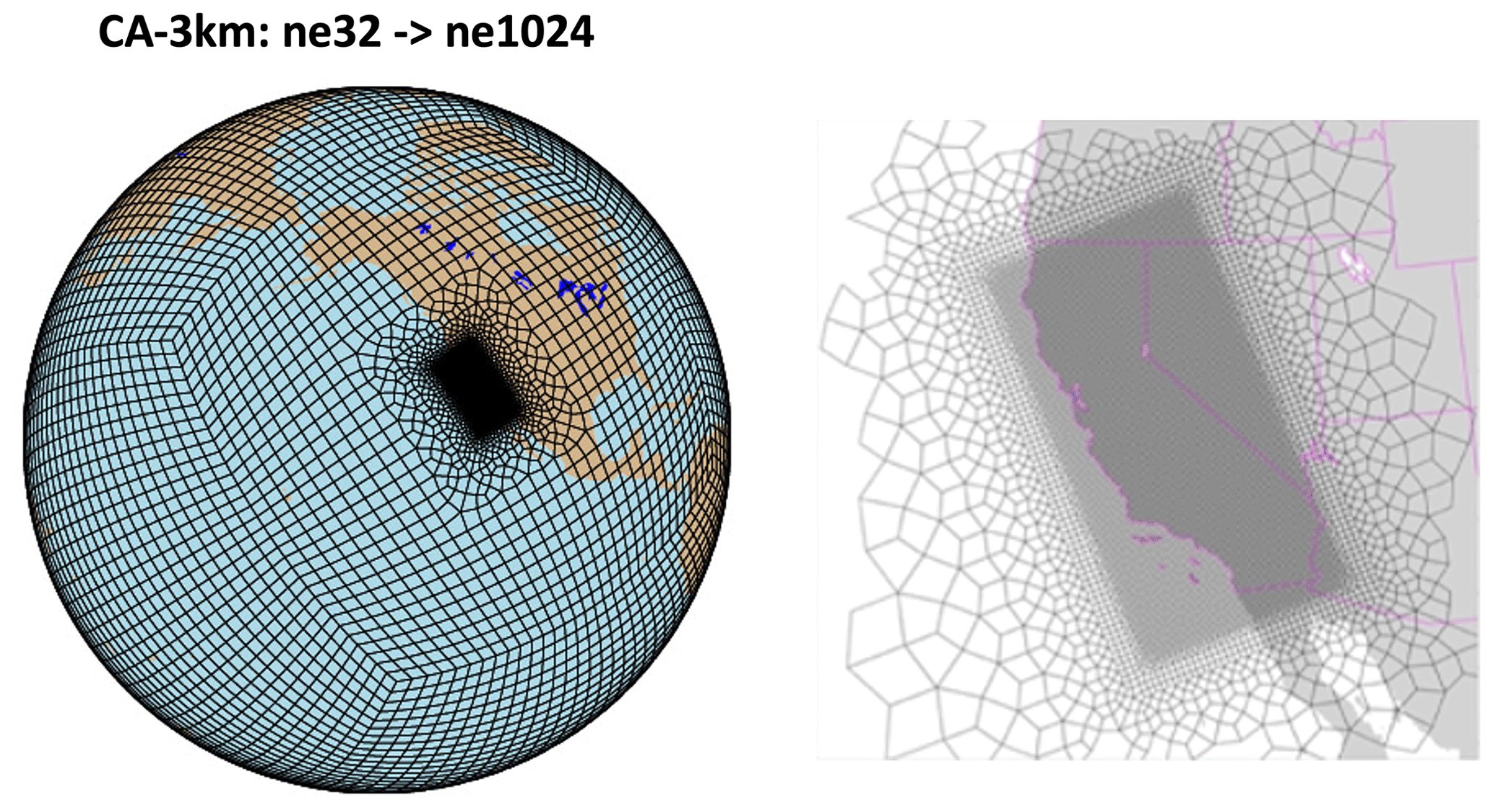
Figure 1Illustration of the grid mesh used for the CA-3km CA RRM grid configuration in this study, featuring a resolution of ne1024 (approximately 3 km) within the refined region and ne32 (approximately 100 km) outside this region.
3.1.1 Refined domain sensitivity
Rhoades et al. (2020) explored the role of the refinement mesh size in CESM and found that resolution over the western US generally played a more important role for accurate simulation of climatological precipitation than the distance of the upstream high-resolution mesh from the area of interest. However, the size of the refined mesh in our control CA-3km grid is far smaller than any refined mesh size tested in Rhoades et al. (2020). The CA-3km grid was designed to encompass the entire state of CA but was intentionally constructed to make the high-resolution region as small as possible to mitigate computational cost for the long-duration simulations. Recognizing that the incoming meteorology to CA could be impacted due to the closeness of the transition region to the state, we construct two grids to explore the potential sensitivity of having a very small RRM. The first we refer to as EPAC-3km (left panel of Fig. 2). Similar to the control CA-3km grid, the resolution of the refined patch is ne1024, while the resolution of the outer global domain is ne32. However, the refined patch has been substantially expanded west into the eastern Pacific Ocean. This allows the transition region to be further away from the area of interest (CA) and is similar to other nested regional models used for CA AR simulations (e.g., Huang et al., 2020). The upstream refined mesh distance from CA for EPAC-3km is also similar to the smallest refined domain used in Rhoades et al. (2020) for CESM.
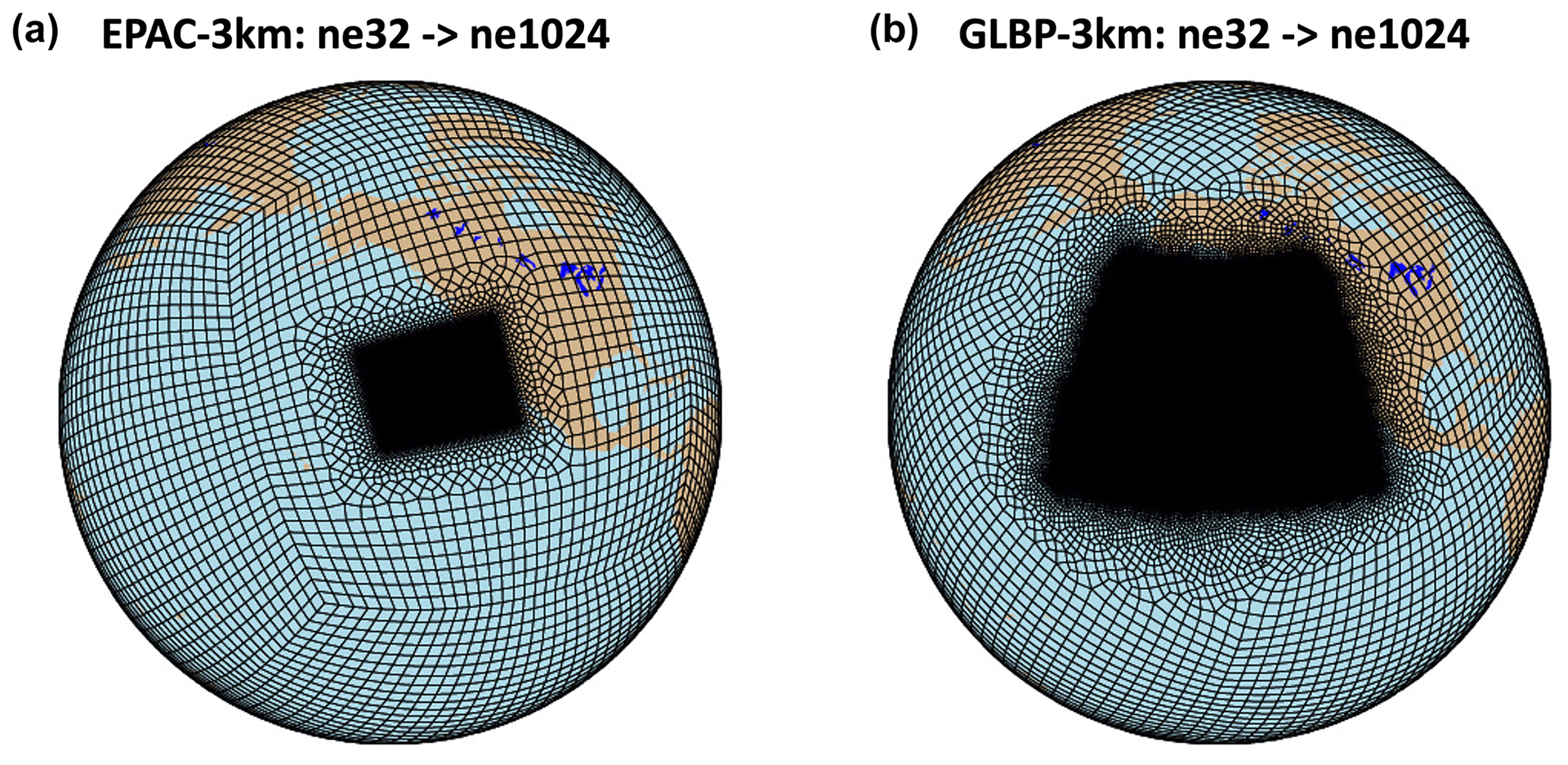
Figure 2Depiction of the grid mesh used for the (a) EPAC-3km and (b) GLBP-3km grid configurations. Both configurations have ne1024 (∼ 3 km) resolution within the refined region and ne32 (∼ 100 km) resolution outside this region.
The second grid designed to test the domain sensitivity is referred to as GLBP-3km (right panel of Fig. 2). This grid has the same resolution specifications in the refined and global regions when compared to the CA-3km and EPAC-3km configurations, but the refined region has been substantially expanded to the north, south, and west, while it is only modestly expanded to the east. We consider this domain to be (and will occasionally refer to it as) our “global proxy”, and it serves as a substitute to running our cases using global 3 km SCREAM to mitigate computational expense. The GLBP-3km grid was deliberately constructed so that all incoming meteorology (i.e., atmospheric rivers and associated storm systems) to CA would be contained within the high-resolution mesh for the entire simulation duration for all cases.
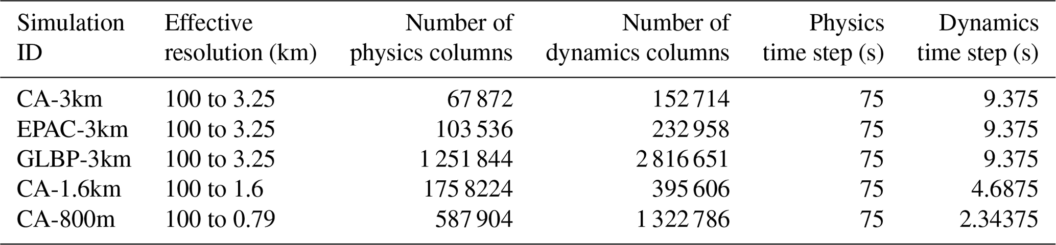
Table 1 summarizes the specifics of the grids used, including the number of columns and the time steps for each configuration. We note that the HOMME dycore consists of spectral elements, with each element containing 4 × 4 grid of Gauss–Lobatto–Legendre (GLL) nodes, while the physics is handled by a uniformly spaced 2 × 2 grid (called “pg2” grid), which substantially increases the model throughput (Hannah et al., 2021).
3.1.2 Refined resolution sensitivity
To test the resolution sensitivity of SCREAM in simulating CA ARs we construct two grids with higher resolution within the refined patch. For both these grids, the areal extent of the refined patch is exactly the same as that in the CA-3km control grid (Fig. 1). However, in one we increase the resolution of the refined patch to ne2048, roughly corresponding to a resolution of 1.6 km, and we refer to this grid as CA-1.6km. For the other grid we increase the resolution of the refined patch to ne4096, corresponding to a resolution of approximately 800 m, and this grid is referred to as CA-800m. Table 1 provides details for the various grid configurations used in this study.
3.2 Atmospheric river event cases
To assess the skill of SCREAM RRM in simulating ARs, we carefully choose four meteorologically distinct events. It it important to clarify that while some of these events may have had significant societal impacts, our selection criteria aimed to assemble a diverse set with varying meteorological setups and regional effects, rather than focusing solely on the most costly or disruptive occurrences. Our chosen cases include two events predominantly affecting northern California: one centered on central California and another making landfall in southern California. The following section provides a brief introduction for each case, along with the rationale behind their selection.
For convenience, we have included Fig. 3, which shows the locations of various California geographic features, various points of interest, and evaluation sites that are frequently mentioned throughout this paper when discussing the cases and results.
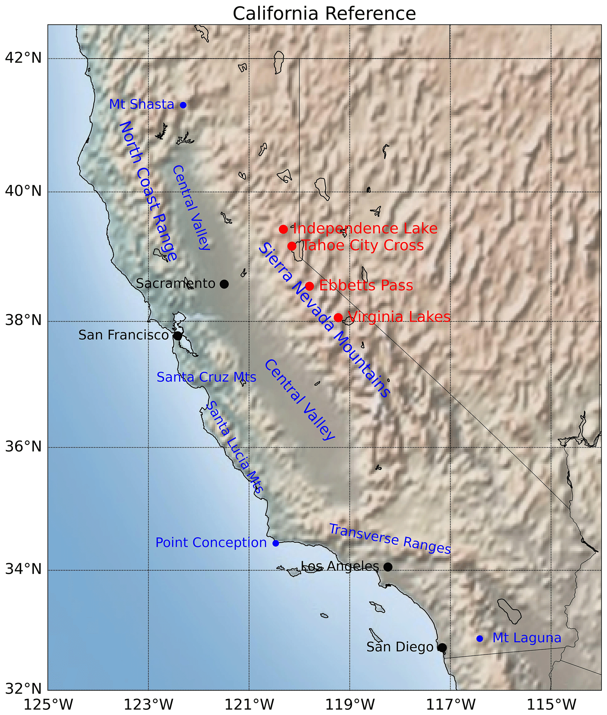
Figure 3Reference map denoting locations frequently mentioned in this paper. Geographic and general points of interest are denoted in blue text, the SNOTEL sites used for comparison against model data are denoted in red text, and major city locations are denoted in the black text.
3.2.1 October 2021 – northern California (NC2021)
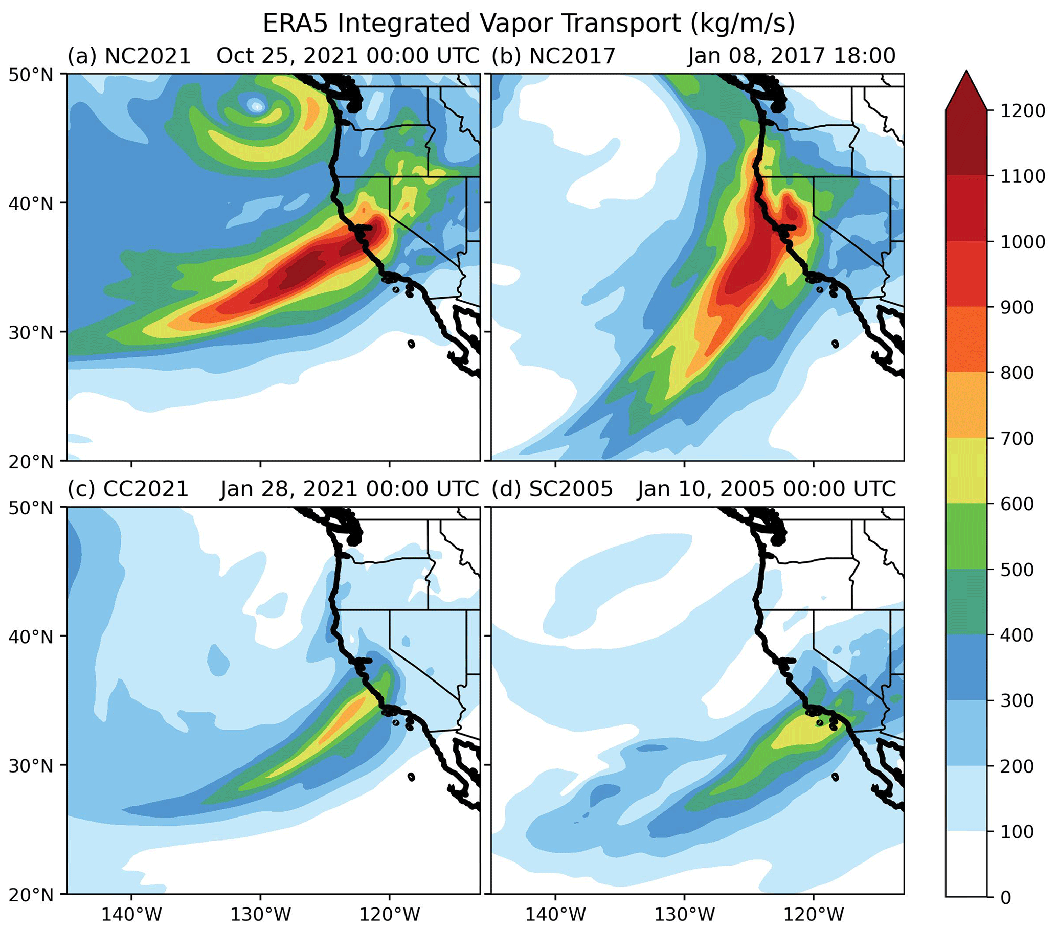
On 24 October 2021 an “exceptional” category 5 (Ralph et al., 2019) AR primarily affected northern CA. This AR was associated with a parent low that underwent rapid intensification in the northeastern Pacific. While the center of this low made landfall well north of CA, this system was associated with a potent and long stream of moisture tapped into the subtropics that was aimed directly at CA. This storm delivered unseasonable and exceptional precipitation accumulations (as high as 375 mm or 14 in.) to northern California and the Sierra Nevada, in addition to widespread reports of damaging winds in excess of 27 m s−1 that resulted in extensive power outages. Two very active fire seasons experienced in CA prior to this event contributed to debris and mud flows as well as flooding in areas of burn scars. Although the higher elevations in the Sierra Nevada experienced a noteworthy amount of snowfall for October, this was predominantly a warm atmospheric river event, with the vast majority of precipitation falling as rain rather than snow over the higher terrain. Figure 4a displays the Fifth Generation European Centre for Medium-Range Weather Forecasts Reanalysis (ERA5; Hersbach et al., 2020) integrated vapor transport (IVT) during peak intensity at landfall on 25 October 2021 at 00:00 UTC.
This marked an unusually potent atmospheric river impacting California, an occurrence that typically transpires once every 5 to 10 years (Ralph et al., 2019). Particularly noteworthy is the timing of this event in October, a period deemed as California's “shoulder season” for precipitation. However, despite the strength of this storm, the hydrologic impacts produced were relatively muted due to the dry antecedent conditions present in state. In addition to being the first major storm of the season, CA was experiencing its most intense drought in recorded history with nearly 60 % of the state classified as D4 or the “exceptional drought” classification (https://droughtmonitor.unl.edu/About/AbouttheData/DroughtClassification.aspx, last access: 29 July 2024). Had this AR occurred in the middle of an active period, such as the recent storm cycles of 2016–2017 or 2022–2023, with a pre-existing snowpack, saturated soils, and reservoirs at maximum capacity, the impacts of this storm would have likely been much more severe (such as in the 1997 CA flood event; Lott et al., 1997). Therefore, it is important to evaluate SCREAM's ability to represent this type of strong and warm AR.
3.2.2 January 2017 – northern California (NC2017)
The 2016–2017 water year was truly exceptional, being one of the wettest recorded for northern California and helping the state escape its longest drought in recorded history. January 2017 was one of the most active periods during this year, responsible for delivering a parade of moderately strong ARs in rapid succession. This series of storms resulted in overflowing rivers, saturated soils, and increased risk of mudslides in areas affected by wildfires in previous years. The Oroville Dam, the tallest dam in the United States, faced a critical situation as its spillway suffered damage, prompting evacuations downstream due to the potential for catastrophic failure. In addition, unlike the NC2021 event, this series of storms produced copious amounts of Sierra snowfall which led to widespread travel disruptions and temporary closures of many ski resorts.
In this study, our focus centers on simulating a 5 d time frame spanning from 7 to 11 January, during which two noteworthy ARs unfolded. The initial AR, which manifested on 8 January, proved to be the more formidable of the two, marked by thunderstorms featuring frequent hail and lightning, the highest cumulative rainfall and snowfall, and the most substantial hydrological impacts. Classified as a category 4 event, it was promptly succeeded by a category 3 AR on 10–11 January. This specific period is chosen to leverage SCREAM's capability to model consecutive and robust AR occurrences, coupled with the substantial snowfall accumulation in the Sierra Nevada. Figure 4b provides a depiction of the IVT during the first AR event on 8 January 2018 at 18:00 UTC.
3.2.3 January 2021 – central California (CC2021)
Opposite to the 2016–2017 water year, the 2020–2021 water year was among the driest ever recorded for several regions of the state. While the storm track was active this year, the large-scale pattern was influenced by a strong La Niña with a Pacific high-pressure ridge that directed the vast majority of storms towards the Pacific Northwest and only bringing California light showers. However, this year did produce one notable storm that was characterized as a cold AR associated with a strong cold front that stalled over the central coast of CA for several days. Localized regions of the Santa Lucia coastal mountain range received upwards of 450 mm (18 in.) of rain for this event, and it washed out sections of the famous Highway 1 in Big Sur. This storm was also notable for not only producing an abundance of mountain snow in the Sierra Nevada but also the relatively rare snow accumulations in the hills of the San Francisco Bay Area and the Transverse Range in southern CA.
Preceding this storm, a ridge of high pressure was sitting over the southeastern Pacific. The anticyclonic rotation of the high pressure pushed a large swath of moisture northward toward Alaska. This moisture was directed around the central high pressure and then southward toward CA on 26–29 January 2021. Therefore this storm was characterized as a “cold” AR, which is fairly atypical as CA is generally more susceptible to “warm” ARs that have a direct connection to moisture from Hawaii or the subtropics. While this storm was not unusually strong (especially when compared to the NC2021 or NC2017 cases), ranking as a category 3 AR, this represents an ideal case study to assess SCREAM's performance in simulating not only an AR with cold origins but also one that stalled over the complex terrain of Big Sur for several days. The IVT as seen by ERA5 on 28 January 2021 at 00:00 UTC as it stalled along the central coast can be seen in Fig. 4c.
3.2.4 January 2005 – southern California (SC2005)
Late December 2004 through early January 2005 was a profoundly wet period for all of California, but this was especially true for the southern reaches of the state. The 7–11 January time period was particularly wet for southern California, with precipitation that continued nearly unabated and caused 10 deaths due to a landslide into homes in a coastal town in Ventura County. This storm was also responsible for causing millions of dollars of flood- and storm-related damage throughout the region, and thus it is probably the most impactful storm included in this study. Isolated areas in the Transverse Mountain Range received upwards of 750 mm (30 in.) of precipitation, with widespread reports of accumulations over 250 mm (10 in.) observed through this range.
The large-scale pattern was characterized by a blocking ridge near the Alaskan Aleutian Islands and a quasi-stationary low-pressure system off the West Coast of the United States, which is an ideal synoptic setup to usher storms into California over a prolonged duration (Benedict et al., 2019; Zhou and Kim, 2019; Carrera et al., 2004). The most crucial ingredient, however, was the intrusion of subtropical moisture delivered via a moist subtropical jet stream that was aimed directly at southern California. Though this AR only briefly achieved a maximum intensity representative of category 3 status, it was the duration of this AR that was responsible for the most significant impacts over southern California. Figure 4d displays the IVT as depicted by ERA5 on 10 January 2005 at 00:00 UTC. In addition, the cold shortwave troughs hitting California from the north and interacting with subtropical moisture helped to produce 7 to 10 ft. (2 to 3 m) of snow in the Sierra Nevada. We include this case because of its impact on the Transverse Mountain Range and to evaluate how SCREAM simulates long-duration stalled AR events.
3.3 Initialization and nudging
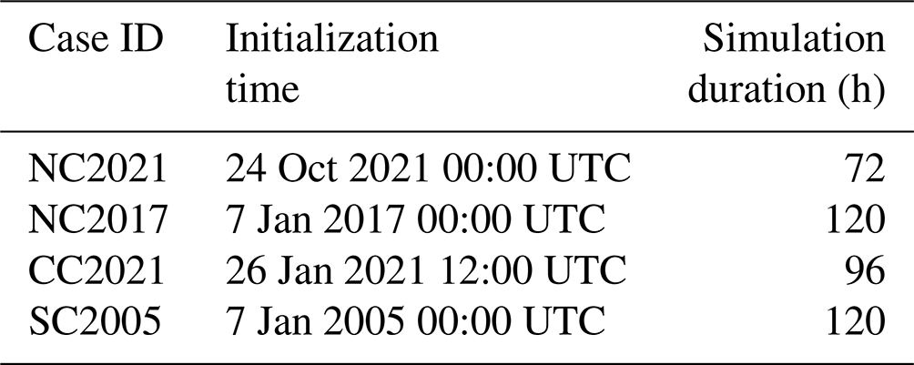
All cases are initialized using ERA5. Each simulation is initialized with reanalysis approximately 24 h before the AR makes landfall on CA. The initialization time and the simulation length for each case are noted in Table 2. We do note that sensitivity tests were conducted for select cases to assess the skill when increased or decreased forecast lead time is applied, and those results will be noted in the Results section. In addition, unless otherwise stated, results for all cases and grid configurations presented are from a single realization. In Sect. 4.4 we discuss the sensitivity of our results when ensemble members are considered.
Table 2Description of atmospheric river cases simulated by SCREAM RRM.
All results presented in this paper are from “free-running” simulations, meaning that no nudging to ERA5 is applied after initialization. SCREAM RRM functionality allows nudging to be applied in select regions of the globe, enabling us to nudge the coarse outer domain while allowing the high-resolution mesh to be freely simulated. When evaluating the initial performance of SCREAM RRM in simulating each case, we performed experiments using the CA-3km grid where nudging to ERA5 was applied in the coarse domain. The results of these experiments differed little when compared to the free-running simulations. Therefore, we decided to only present results of the free-running simulations to eliminate any uncertainty that might be introduced in our nudging strategy (i.e., sensitivity to nudging timescales, etc.).
3.4 Evaluation data
To conduct a thorough assessment of AR events in California, it is crucial to compare them against observational datasets with ample temporal and horizontal resolution. This strategy is important as the expected advantages of high-resolution simulations are more likely to become apparent on smaller temporal and spatial scales. To evaluate the simulation of precipitation and temperature, we use the 4 km PRISM (Parameter-elevation Regressions on Independent Slopes Model) dataset (PRISM Climate Group, Oregon State University, https://prism.oregonstate.edu, last access: 16 December 2020). The PRISM dataset adopts the philosophy that “elevation is the most important factor in the distribution of climate variables” for a localized region. For example, PRISM utilizes regression functions correlating precipitation and elevation within specific categories, distinguished by slope orientation. This differentiation enables a precise evaluation of precipitation on both windward and leeward slopes.
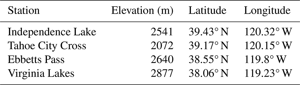
To assess the snow water equivalent (SWE), we employ assimilated snow observations provided by the University of Arizona (UA). The UA SWE dataset (Zeng et al., 2018), sourced from in situ measurements within the Snow Telemetry (SNOTEL; https://nwcc-apps.sc.egov.usda.gov/imap/, last access: 29 July 2024) network and Cooperative Observer Program (Leeper et al., 2015), integrates temperature and precipitation data from PRISM. This extensive 40-year dataset boasts a spatial resolution of 4 km. To evaluate large-scale variables, such as integrated vapor transport (IVT), we use the ERA5 global reanalysis (Hersbach et al., 2020). In addition to the observation-based gridded UA product we also compare select points to the SNOTEL network. We choose four sites to compare to (Table 3): Independence Lake, Tahoe City Cross, Ebbetts Pass, and Virginia Lakes. All four sites are found in the Sierra Nevada mountain range; the first two are fairly close to each other, straddling the I-80 corridor, but differ by more than 450 m (1500 ft) in elevation. Ebbetts Pass and Virginia Lakes sites are both found in the central Sierra Nevada, with the former located at pass level and the later located on the lee side of the mountain range. Though the Ebbetts Pass site is located at pass level, the Virginia Lakes site sits on a ridge and is actually at higher elevation compared to Ebbetts Pass.
Table 3Elevation and location information for the SNOTEL sites used for observational reference.
We primarily evaluate the proficiency of the SCREAM RRM in simulating California ARs by emphasizing its capability to replicate observed patterns of accumulated precipitation and snowfall. Additionally, we examine how well the model captures the structure and magnitude of integrated vapor transport (IVT) throughout the duration of the events. Figure 4 illustrates the integrated vapor transport (IVT) during peak intensity as observed in the ERA5 reanalysis for each case. Conversely, Fig. 5 presents the corresponding information for SCREAM simulations conducted on the CA-3km grid. The analysis of the two figures reveals that, overall, SCREAM effectively reproduces the magnitude and structure of IVT compared to ERA5 reanalysis, albeit with some discernible discrepancies. In the NC2017 case, SCREAM exhibits a slightly heightened IVT magnitude offshore but weakened magnitudes inland. Conversely, in the SC2005 case, the SCREAM-simulated IVT appears somewhat narrower and more intense, in contrast to the broader and relatively weaker magnitudes observed in the ERA5 IVT. Examining the IVT structure at one simulated time, however, is quite limiting and a more comprehensive analysis of the simulated IVT will be examined in greater detail. This comparison is presented to demonstrate the general characteristics of the simulated IVT by SCREAM RRM on the CA-3km control grid.
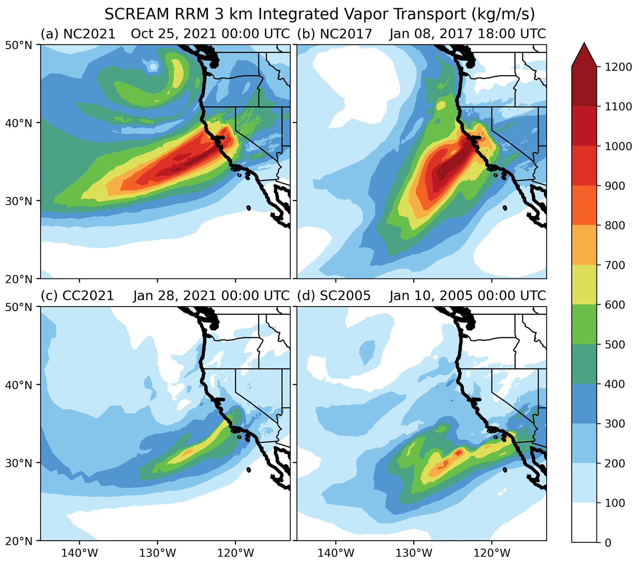
Figure 5Same as Fig. 4 but for SCREAM RRM CA-3km simulations.
4.1 Accumulated precipitation
The event accumulated precipitation skill scores, comprised of the root mean squared error (RMSE), bias, and correlation coefficient for each case and for all grid configurations, are displayed in Fig. 6. We note that all skill scores presented are statewide, using only the model columns and points for SCREAM and PRISM that fall within California. These are determined by a mask file generated from a California shapefile. For all scores and cases, PRISM is used as the observational data source. One key takeaway from this figure is the proficiency of SCREAM in representing the warm AR of NC2021. While it is apparent that SCREAM suffers from a statewide positive precipitation bias for all cases and grid configurations, this bias is muted for the NC2021 case. Conversely, SCREAM has the least skill in representing the relatively colder (and successive) AR events that occurred in the NC2017 case.
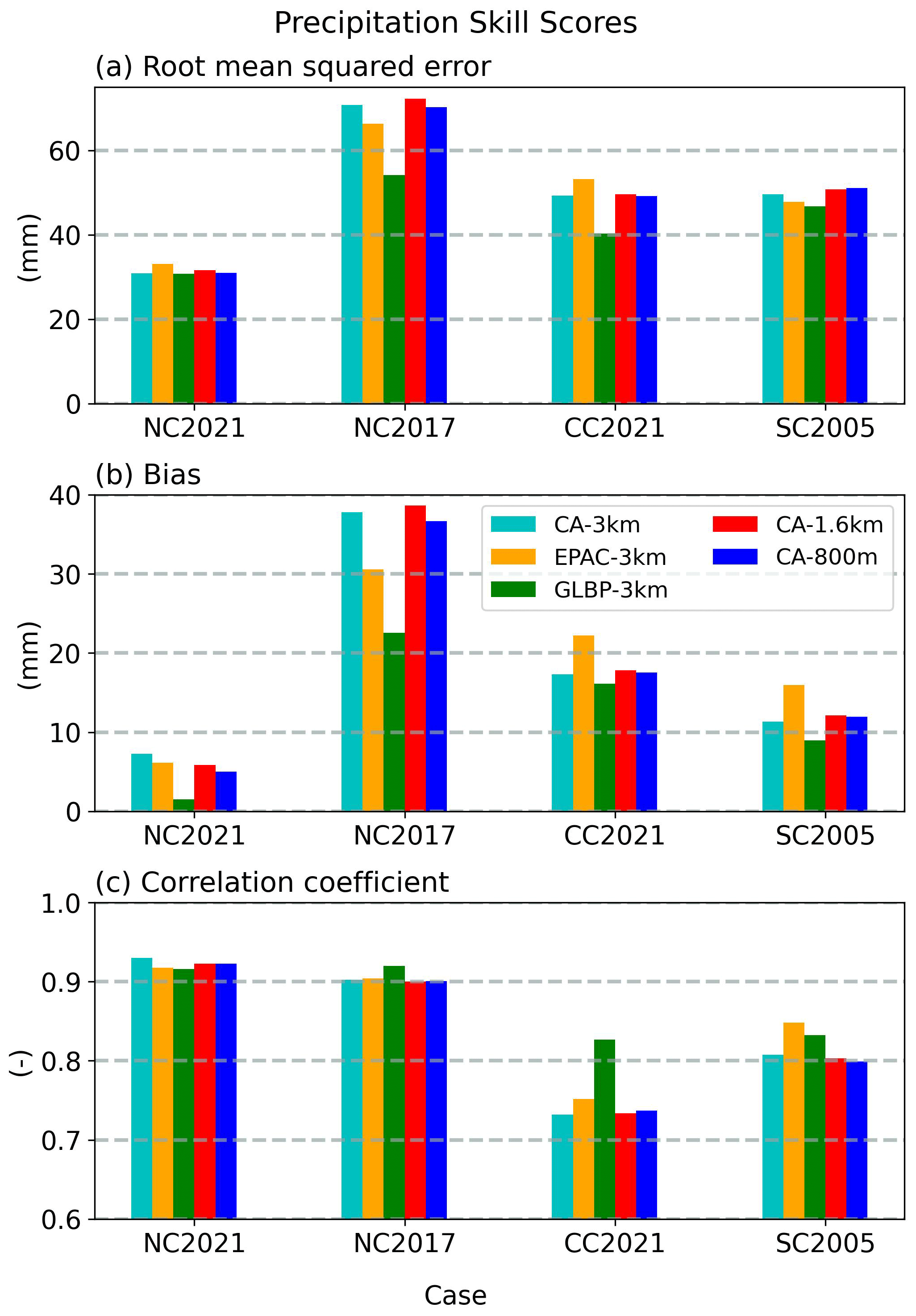
Figure 6Skill scores for the event accumulated precipitation for each case and grid configuration as computed with respect to PRISM observations. Displayed are the (a) root mean squared error, (b) bias, and (c) Pearson pattern correlation coefficient.
An observation evident from Fig. 6 is that resolution seems to have a minimal impact on precipitation skill. For instance, the CA-1.6km (ne2048) and CA-800m (ne4096) grids do not demonstrate improved skill scores when compared to the CA-3km grid, though it should be noted that to compute the skill scores all grids were remapped to the PRISM grid, which is a bit lower-resolution than the CA-1.6km and CA-800m grids. There can be implications when interpreting these skill scores when the model resolution goes beyond the observations (Risser et al., 2019).
Perhaps the most interesting piece of information inferred from Fig. 6 is that most grid configurations generally cluster around one another, with a couple notable exceptions. Chiefly, for the CC2021 cold AR case and the NC2017 case we note that the GLBP-3km grid (which serves as our global high-resolution proxy) exhibits comparatively greater skill. Specifically, most grid configurations tend to have the lowest Pearson pattern correlation scores for the CC2021 case; however, the “global proxy” grid is an outlier. Additionally, in the NC2017 case we see that the GLBP-3km grid has noticeably smaller RMSE and bias scores.
To gain a deeper understanding on the characteristics of regional precipitation distributions in SCREAM RRM, we examine the observed versus simulated event accumulated precipitation in Fig. 7. Since we found that most SCREAM RRM grid configurations tend to cluster around one another, we display three select grids, specifically the CA-3km, CA-800m, and GLBP-3km grids. While Fig. 7 displays the event accumulated precipitation, this figure is complemented by Fig. 8, which displays the regional biases for each grid configuration. We refer to both figures in tandem for the following analysis, in which we will systematically discuss results for each individual case.
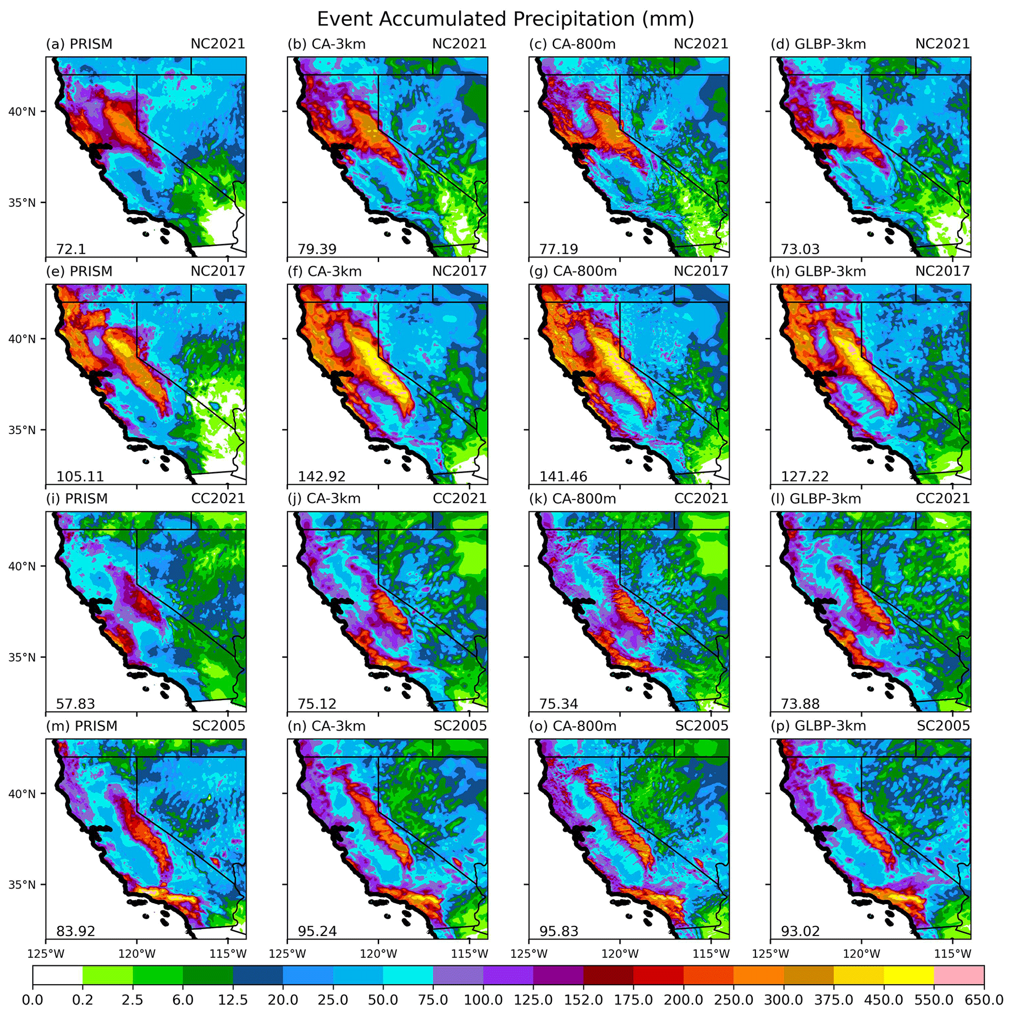
Figure 7Event accumulated precipitation for (top row) NC2021, (second row) NC2017, (third row) CC2021, and (bottom row) SC2005. Displayed are the (left column) PRISM observations, (second column) CA-3km RRM configuration, (third column) CA-800m configuration, and (right column) GLBP-3km grid configurations. The numerical value in the bottom left corner of each panel depicts the averaged value for CA. All data are plotted on the observation or model native grid.
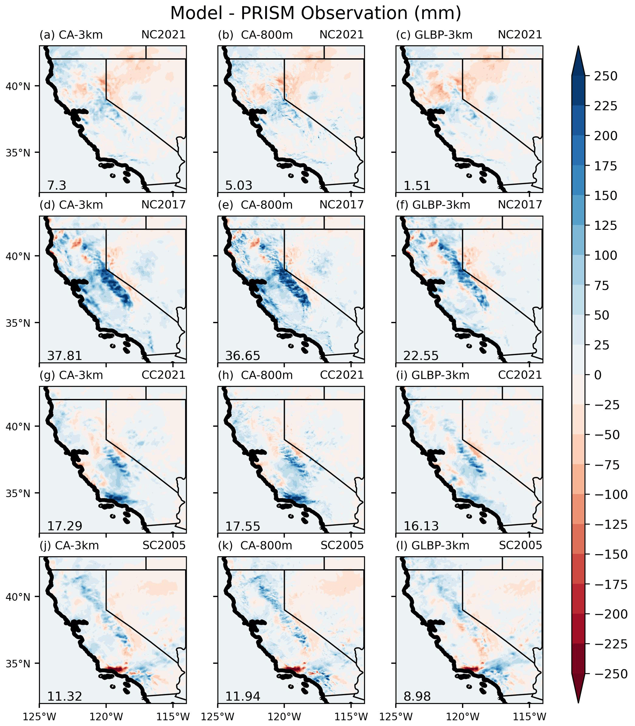
Figure 8Event accumulated precipitation bias computed relative to PRISM observations for (left column) CA-3km RRM, (middle column) CA-800m, and (right column) GLBP-3km for each case. The numerical value in the bottom left corner of each panel represents the averaged bias over CA. Model simulations are remapped to PRISM resolution to compute bias.
The top row in Figs. 7 and 8 confirms the satisfactory and robust performance of SCREAM RRM in the simulation of the category 5 warm NC2021 case. Evident in all three grid configurations shown is a good representation of the regional precipitation distributions, with a maximum along the northern Sierra Nevada mountain range, secondary maximum along the north coastal ranges, and minima in the central valley. The relatively more modest precipitation totals in central and southern California are well represented in addition to precipitation maxima of the smaller mountain ranges, such as the Santa Cruz Mountains. Figure 8 (top row) reveals that all configurations have a positive precipitation bias in areas of topography (most conspicuous in the Sierra Nevada range) and dry bias in valleys and areas downwind of topography (i.e., the northern CA central valley and western Nevada) for this case. Though the GLBP-3km simulation has a statewide mean precipitation accumulation that agrees best with observations, it is evident from Fig. 8 that this is largely due to compensation for a stronger central valley dry bias when compared to the other grid configurations.
Regional precipitation distributions and biases for the NC2017 case are displayed in the second row of Figs. 7 and 8, respectively. As already discussed, this is the case where all SCREAM RRM configurations tend to deliver the poorest precipitation skill scores. This is made evident by the large precipitation biases, though as already pointed out, these biases are muted for the GLBP-3km grid. The majority of the positive precipitation bias in the CA-3km and CA-800m cases is centered on the Sierra Nevada, with large biases also seen in coastal central California (i.e., the San Francisco east Bay Area and Big Sur region). In the GLBP-3km grid the Sierra Nevada bias is still prominent yet substantially reduced, while the biases in the east Bay Area and Big Sur regions are largely eliminated, both of which are responsible for the improved skill scores for this grid. However, it should be noted that all grid configurations perform well for the northern coastal range areas.
Unlike the two previous cases in which northern California was the focus of the landfalling ARs, the CC2021 represents a case in which a strong AR stalled over central California (third row of Figs. 7 and 8). Also unlike the NC2021 and NC2017 cases, most grid configurations suffered from lower pattern correlation scores. This is evident when examining the regional precipitation distributions. PRISM observations show well-defined maxima over the Santa Lucia coastal mountains in central CA and the southern Sierra Nevada mountains. While all SCREAM RRM configurations represent the spatial distribution of the Sierra maxima (albeit with a positive bias), the coastal maxima is displaced to the south over the Transverse Mountain Range in the CA-3km and CA-800m grids. While the GLBP-3km grid also has a wet bias over the Transverse Mountain Range, the placement of the geographically small maxima along the central coast is well represented. This is another interesting difference (improvement) pertaining to the GLBP-3km grid that will also be discussed in further detail.
The bottom row of Figs. 7 and 8 displays the accumulated precipitation and associated biases, respectively, for the long-duration AR event that was focused on southern CA. PRISM observations show observed maximum precipitation along the Transverse Range in Ventura County, with another maximum associated with the more inland ranges (i.e., San Gabriel and San Jacinto mountains). While all configurations represent the maximum of the inland mountain ranges well, all fail to capture the absolute maximum in the Transverse Range, as evidenced by a localized dry bias larger than 250 mm (which represents the worst local bias for all of the cases included in the study). This is not too surprising when comparing the simulated IVT to that of reanalysis (Figs. 4 and 5), which showed that SCREAM's moisture plume was too narrow for this case. It is interesting that neither resolution nor refined domain size improves this representation, and it is worthwhile to note that Huang et al. (2020) simulated this same case using WRF, which also had a substantial dry bias in the Transverse Range. While the Sierra Nevada received significant precipitation during this event, that precipitation was largely attributed to several passing short waves during this time period aided by weak AR moisture. However, it is interesting to note that the Sierra precipitation bias for this case is far muted when compared to the CC2021 and NC2017 cases.
While each case certainly contains its own unique regional precipitation characteristics and model biases, some common themes and connections to other work can be made. First, it is apparent that SCREAM tends to overestimate precipitation related to topography that is fueled by a large-scale moisture source. For all cases examined, there is a modest to strong precipitation bias over both the major and minor mountain ranges of CA. This is complemented by a prominent dry bias downwind of topography and is most apparent along the CA–NV border east of the Sierra Nevada. Another common theme is the positive statewide precipitation bias, which ranges from 10 % to 35 % depending on the case. This is in comparison to the climatological precipitation bias produced by the CA-3km grid (Zhang et al., 2024) of 129 %. Zhang et al. (2024) hypothesized that the strong precipitation bias in their simulations was attributed to a combination of errors in the large-scale forcing (which was nudged to a 100 km E3SMv1 run in the coarse outer domain) and biases in the SCREAM physics. The smaller biases produced in our hindcast simulations suggest that a majority of the bias produced by SCREAM RRM climate runs likely stems from the former, with relatively smaller contributions by the later. GCMs typically underestimate the strength and duration of high-pressure blocking ridges that dominate the dry years in California (Davini and D'Andrea, 2020; Schiemann et al., 2020), which likely led to higher-than-observed frequency of storms in the CA RRM downscaled simulations performed in Zhang et al. (2024).
Further, it is interesting to note the lack of importance of resolution in SCREAM RRM AR simulations. In a sense, it is a positive result that SCREAM is not dominated by undue resolution sensitivity and is consistent with the findings of Bogenschutz et al. (2023a), who found SCREAM to be insensitive to resolution for grid box sizes ranging from 800 to 5 km in a doubly periodic configuration. It was not until resolution approached that of large eddy simulation (LES) that they noted a sensitivity, but this was only noticeable in the shallow convective regime. However, their simulations did not include topography. While our simulations show that precipitation can be better resolved in areas of fine-scale topography, there is no discernible benefit in terms of skill scores and bias reduction when moving to 800 m resolution. Finally, it appears that increasing the area of the refined mesh yields improvements over the CA-3km grid, but this is only true if the mesh is substantially refined beyond what is typical for an RRM. We note that these results (pertaining to the importance of resolution vs. refined domain size) are opposite to the conclusions found in Rhoades et al. (2020), who ran various grid configurations with a 25 km refined mesh for the western United States. However, we test grids with smaller refined mesh sizes and with much higher resolution. Combining our findings with those of Rhoades et al. (2020) and Huang et al. (2020) indicates that prioritizing resolution is crucial until approximately 3 km is attained. Beyond this point, enhancing the upstream refined mesh size may yield some incremental improvements, though we do recognize that comparing our results to other works (such as Rhoades et al., 2020, and Huang et al., 2020) we are agnostic to model differences that may not warrant a direct comparison, such as different physics, dynamical core, and vertical levels, for example.
4.2 Accumulated snowfall and temperature
The snowpack plays a crucial role in California's water resource management. Given the distinct intermittence of precipitation in the state, marked by dry summers and comparatively wet winters, the mountain snowpack serves as California's “frozen reservoir”. This essential reservoir aids in generating runoff and mitigating wildfire risk during the dry season (Bales et al., 2011). Therefore, in order to adequately assess changes in snowpack for greenhouse gas emissions, a climate model should be able to simulate the CA snowpack with fidelity. Zhang et al. (2024) found that the CA RRM produced superior skill in simulating the snowpack when compared to the 100 km E3SM. The latter, being too coarse, failed to capture discernable snow patterns essential for assessing climate risks. While Zhang et al. (2024) found that the CA RRM overestimated the climatological snowpack when compared to observations, this is not surprising given the tendency for their model to overestimate precipitation. Here we evaluate SCREAM's ability to simulate the accumulated snow for our AR events.
Figure 9 displays the skill scores for all of our grid configurations for the event accumulated water-equivalent snow depth. To compute these scores we use the University of Arizona snow water equivalent (SWE) as described in Zeng et al. (2018). While it is unsurprising, we note that the bias and RMSE scores for SWE closely mirror those for the total precipitation rate. While SCREAM RRM has nearly zero bias for the warm AR NC2021 case, relatively larger biases are seen for the remaining cases. It is worthwhile to note that the GLBP-3km grid has a very low bias for the NC2017 case for which all other grid configurations overestimate. In fact, similar to the scores of total precipitation (Fig. 6), the GLBP-3km grid tends to score best (albeit by a modest amount for most cases) compared to the rest of the grid configurations. In general, all 3 km (ne1024) configurations score similar for all cases in terms of correlation, while the higher resolutions have somewhat less skill, which could stem from capturing smaller-scale variations in the snowfall distributions that may not be present in a relatively coarser-resolution dataset (Lundquist et al., 2019).
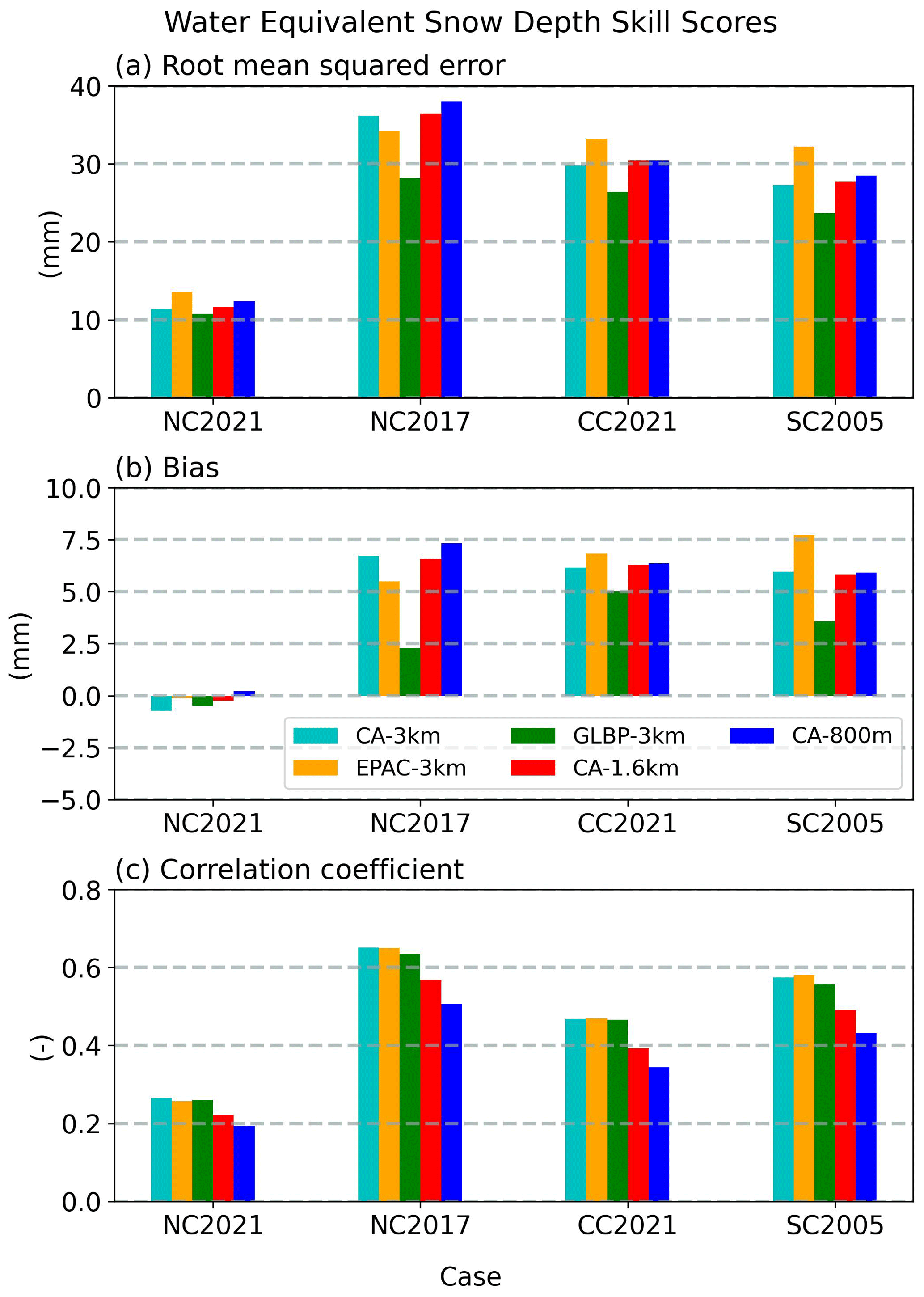
Figure 9Same as Fig. 7 but for water-equivalent snow depth computed according to the University of Arizona observational dataset.
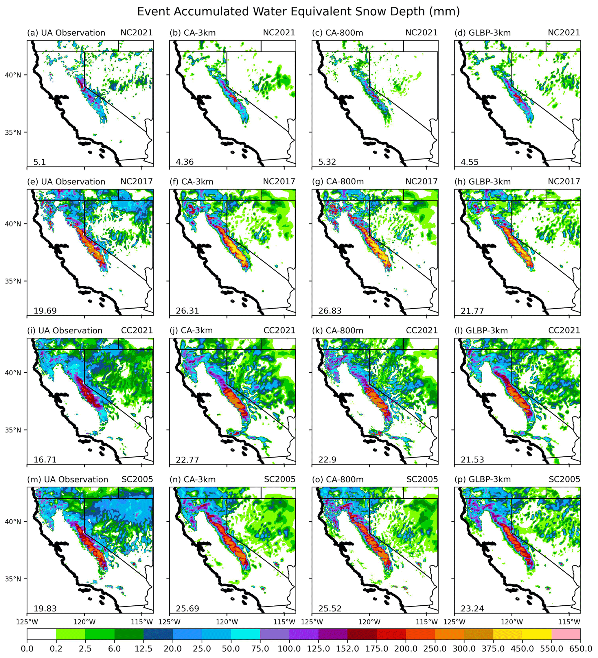
Figure 10Same as Fig. 7 but for water-equivalent snow depth.
The regional distributions of the event accumulated SWE are displayed in Fig. 10. Similar to the precipitation distributions, we only display the observations and the CA-3km, CA-800m, and GLBP-3km grid configurations. Here we focus on some key general points; the first is that for all cases each grid configuration adequately represents the regional distribution of snow in the Sierra Nevada mountain range, though generally with a positive bias. The 3 km and 800 m resolution simulations are able to capture precipitation maximum and minimum associated with individual ridges and valleys within the Sierra Nevada, though we note that this distinction is often overdone within the model when compared to the observations. Once again, this provides evidence of the model's tendency to overestimate precipitation in areas of topography. This is further illustrated by examining the snowfall amounts on the leeward side of the Sierra Nevada, where all cases and configurations have a negative bias in far western Nevada.
Figure 10 also highlights the ability of SCREAM RRM, for all resolutions and configurations, to simulate the fine-scale details relating to topography. This is most apparent when viewing the snowfall amounts in the relatively lower-elevation mountains of the Cascades in northern California. Additionally, for the cold AR associated with the CC2021 case, we see that all configurations are able to capture the very small areal extent of the low-elevation snowfall in the Santa Lucia mountains (central California, Big Sur region) and the Transverse Mountain Range in southern California. The proficiency of SCREAM RRM in accurately capturing intricate details is positive not just for simulating climate impacts specific to California but also for its broader applicability in global SCREAM simulations. It is also interesting to note that while some of the fine-scale details are resolved more sharply in the 800 m (ne4096) case, there is no obvious benefit seen in any cases to using a higher-resolution grid in terms of bias reduction. Again, we note that these high-resolution grids are being compared to observational datasets at a coarser resolution. We will discuss the resolution implications further in the “Discussion and summary” section.
A comparison of all grid configurations to SNOTEL observations for each case at select sites can be found in Fig. 11. The Independence Lake and Tahoe City Cross sites are both in the northern Sierra Nevada and fairly close to one another, though they differ by 450 m (1500 ft) elevation. The Independence Lake site generally receives greater precipitation and snow amounts than Tahoe City and this is true for the SNOTEL observation for all cases. Each grid configuration can capture the distinction between these two sites well, though all seem to underestimate the SWE for the NC2021 case at Independence Lake. Both the Ebbetts Pass and Virginia Lakes sites are located in the central Sierra, with the former at pass level and the latter on a ridge on the lee side of the mountain range. Therefore, Virginia Lakes tends to receive less precipitation relative to Ebbetts Pass, despite being at higher elevation. This is reflected in the SNOTEL observations for each case, and generally this distinction is well captured by the model configurations; the exception is the NC2017 case for the CA-1.6km and CA-800m simulations, which greatly overestimate the SWE compared to SNOTEL. This is important to note because in general there appears to be no obvious advantages seen in the higher-resolution runs for other cases and/or locations, even when comparing to site-specific observations. It is interesting to note that the EPAC-3km configuration generates more snow at all sites compared to the other configurations. This aligns with the slightly higher positive bias observed in statewide precipitation and snow (Figs. 6 and 9, respectively) for this configuration.
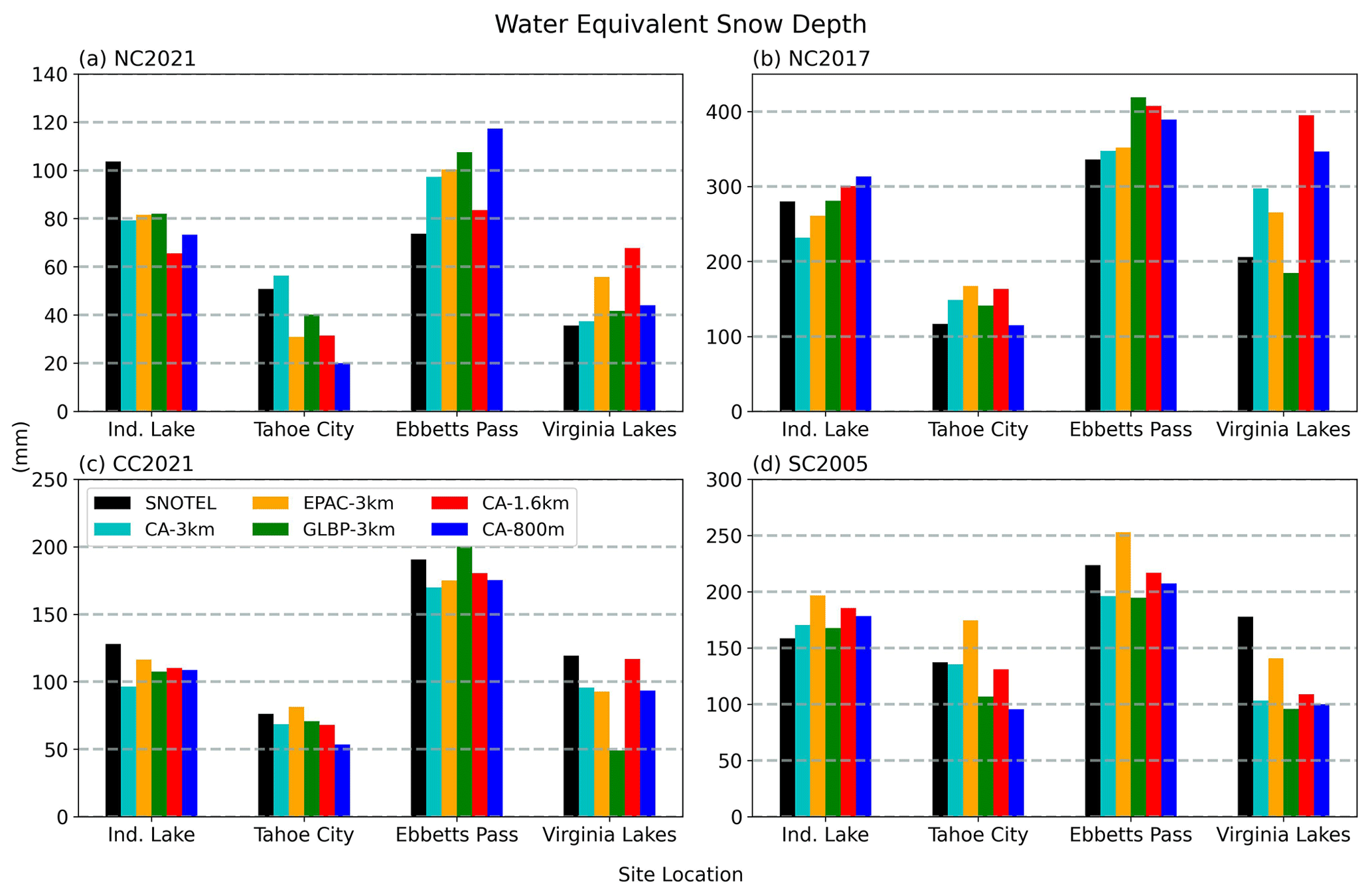
Figure 11Event accumulated water-equivalent snow depth for each case and grid configuration, compared to SNOTEL observations, at four different site locations. Elevation and location for each location can be found in Table 3. Data from model simulations are taken from the native grid.
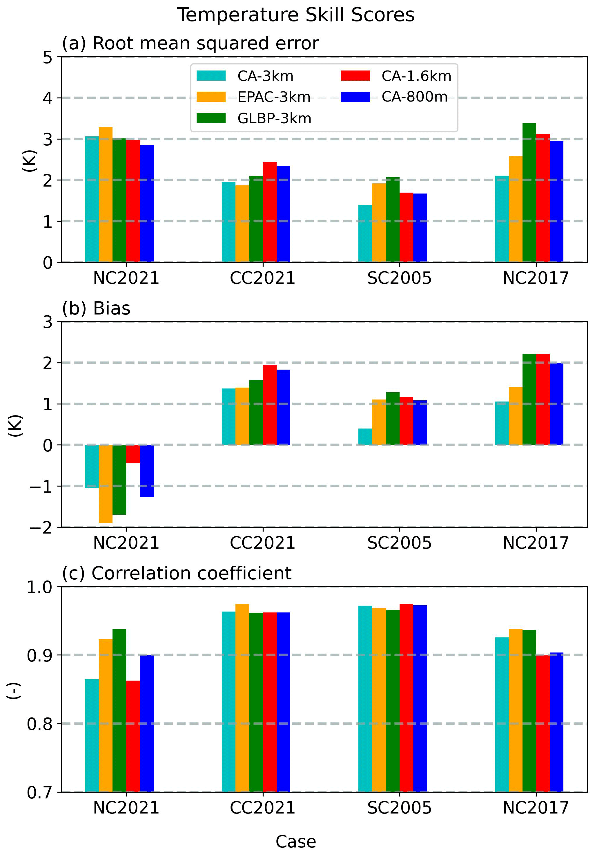
Figure 12 displays the skill scores for the averaged daily 2 m temperature, computed relative to PRISM. In general we see that all grids and configurations have high correlation scores, demonstrating the model's ability to represent temperature patterns across the complex terrain of California (as demonstrated in Zhang et al., 2024). With the exception of the NC2021 case, all experiment configurations and cases exhibit a positive temperature bias. This positive temperature bias is consistent with Caldwell et al. (2021), who showed that SCREAM suffers from a global average 0.7 K positive temperature bias, which is most prevalent over land. It is interesting that the only case which does not have a positive temperature bias (NC2021) also does not have a positive precipitation bias.
4.3 Large-scale moisture flux
Though high resolution is important to capture the topographic effects and accurate regional distributions of precipitation (Huang et al., 2020), a high-fidelity simulation of the synoptic-scale IVT associated with ARs is also a crucial ingredient. When constructing the CA-3km grid for long-term climate projections, concerns were raised about both the abruptness and closeness of the grid transition to CA. Though 100 km is sufficient to resolve the IVT associated with ARs and Bogenschutz et al. (2023a) show that SCREAM is a reasonably scale-aware and insensitive model for idealized cases, it is worthwhile to determine the fidelity of the simulation of the IVT as the grid transitions from 100 to 3 km (and 800 m) compared to reanalysis and the GLBP-3km global high-resolution proxy configuration.
Figures 13 and 14 display the regional distributions of the event maximum and mean IVTs for all events for ERA5 and the selected grid configurations. We note that the temporal resolution of ERA5 is coarser (3 h) compared to the 1 h resolution used in the SCREAM analysis. The maximum and mean values represent the respective values for each grid column for model and analysis. Among the general conclusions gleaned from these two figures is that all configurations have satisfactory representation of the mean and maximum IVT with reasonable regional distributions. Though it should be noted that all SCREAM simulations are much higher-resolution over CA when compared to ERA5, one bias that is obvious is the underrepresentation of the maximum IVT on the leeward side of the Sierra Nevada mountain range. This is consistent with analysis of precipitation and snowfall, showing a strong bias of SCREAM to intercept excessive moisture in areas of topography.
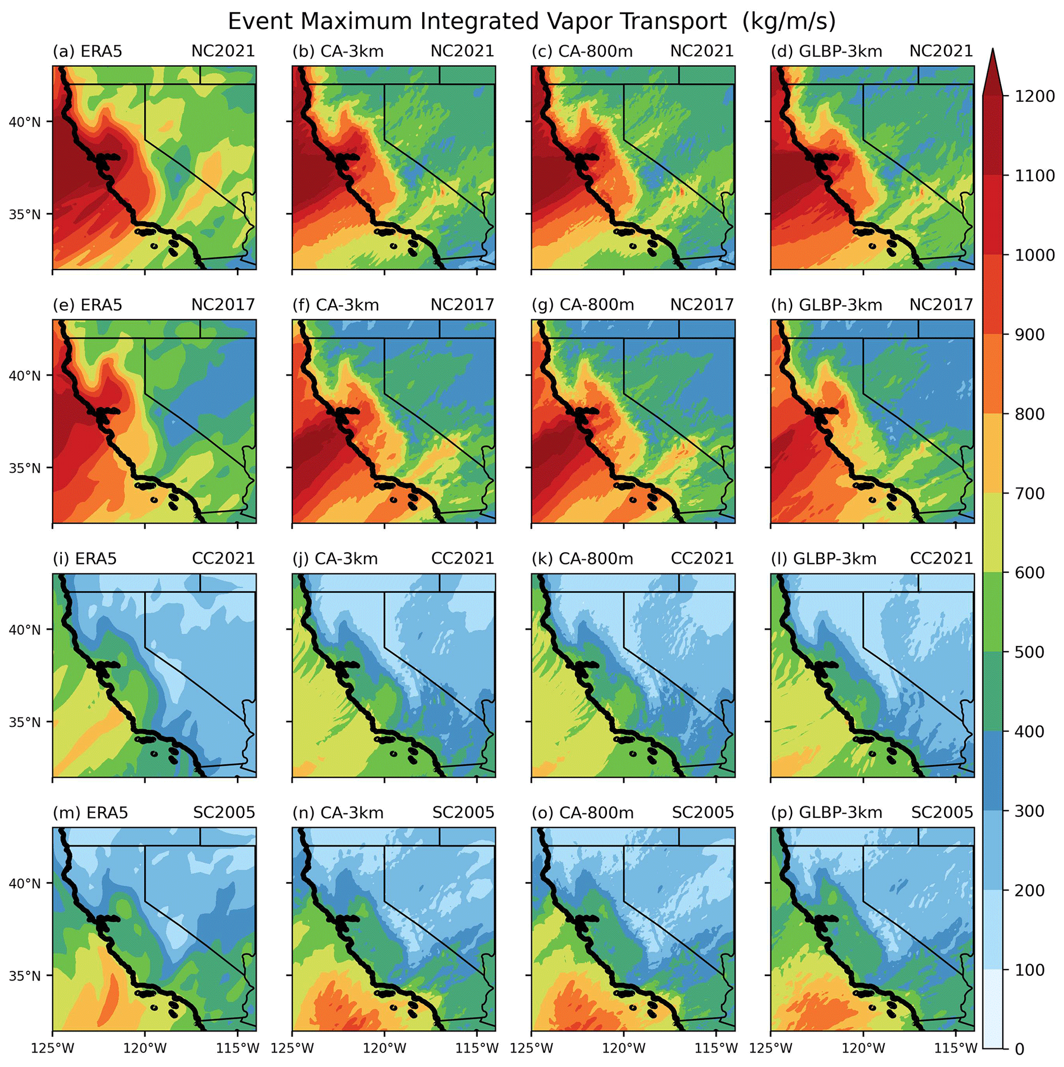
Figure 13Same as Fig. 7 but for the event maximum integrated vapor transport with (left column) ERA5 depicted as the observational reference.
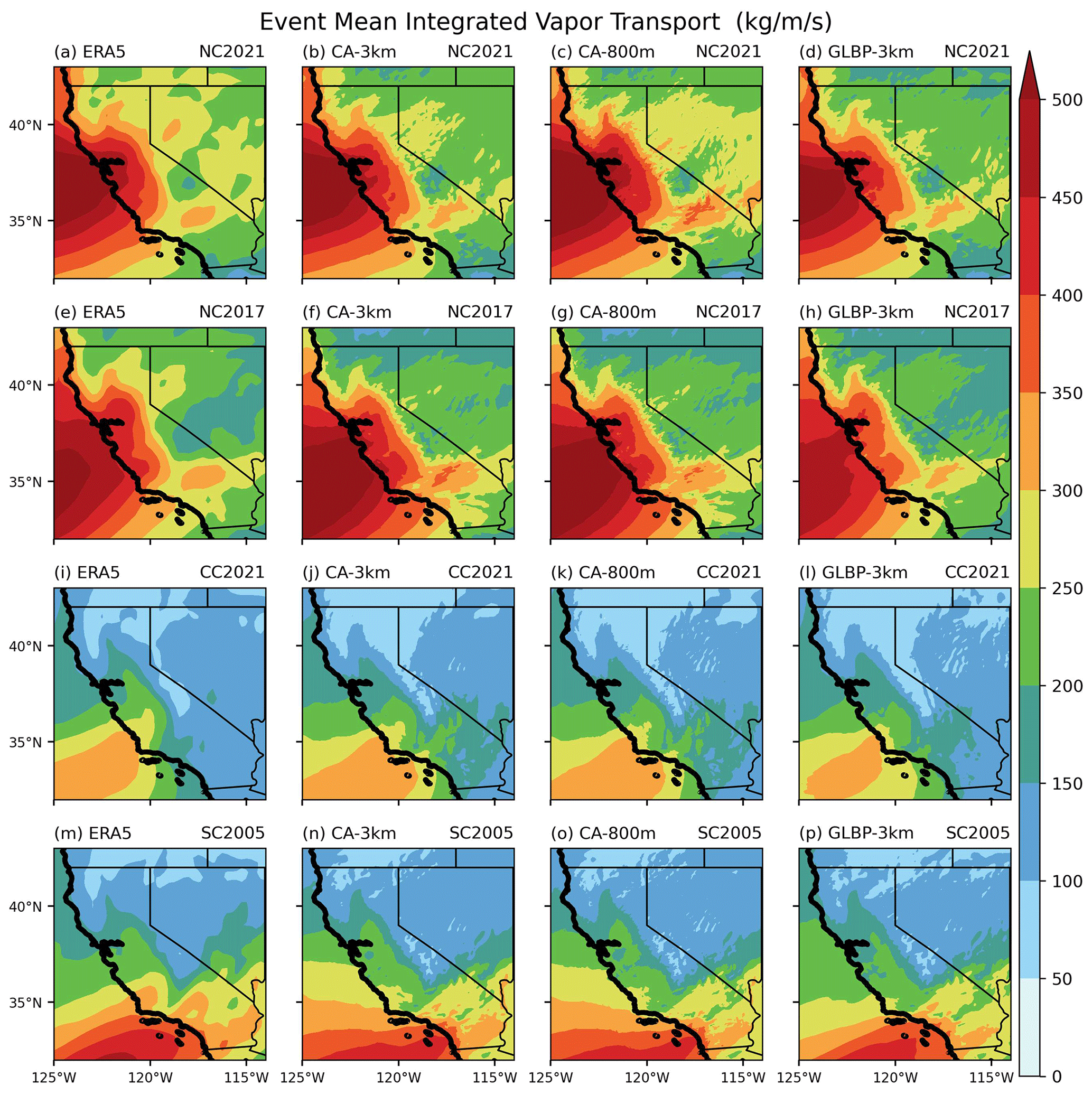
Figure 14Same as Fig. 13 but for the event mean integrated vapor transport.
Though the EPAC-3km and CA-1.6km simulations are not displayed, their results and characteristics are very similar to the CA-3km simulation. One outlier is the GLBP-3km configuration, which tends to produce lower values of the maximum and mean IVT when compared to ERA5; this is most apparent when examining the NC2017 case. This is interesting because NC2017 was the case where GLBP-3km had improved skill scores, especially pertaining to the reduction in bias, when compared to the other simulations. This could suggest that the improved bias reduction of the GLBP-3km simulation could stem merely from compensating errors. When examining the SC2005 case, it is clear that all grid configurations underestimate the event mean IVT at Point Conception (the prominent “kink” in the CA coastline at approximately 34° N; bottom row of Fig. 14). This is consistent with previous analysis which showed that all grid configurations were unable to represent the absolute maximum precipitation observed on the Transverse Range for this case due to the fact that all configurations simulate an IVT plume that is more narrow than observed (as seen in Fig. 5d for the CA-3km control configuration). Nonetheless, despite some regional deficiencies, it is encouraging to note that the structure and magnitude of the simulated IVT are fairly robust among the different configurations which have varying resolutions and refinement locations, with no obvious imprints of the grid transitions present.
While Figs. 13 and 14 provide no information pertaining to the timing and propagation of the IVT plumes through CA, we found that there is virtually no difference in this regard among nearly all grid configurations and cases. The one exception is the CC2021 event where the AR stalled over the central California coast (near Big Sur) for over a day. While all grid configurations feature a stalled AR for this case, this tends to occur a bit further south than observed in most grid configurations over the Transverse Mountain Range. This is reflected in the shifted precipitation maximum in most grids compared to observations and relatively poor pattern correlation scores. The exception is the GLBP-3km grid, which does successfully stall the AR in the correct location. The chief reason for this stall was a region of high pressure near the southern tip of Baja California, in which a subtle southward error placement of this ridge due to the coarse resolution of 100 km grids in the outer domain helped to drive the IVT maximum further south than observed. The GLBP-3km grid, on the other hand, is able to better resolve the large-scale pattern and hence helps to predict the correct placement of the stalled AR. This is an example of how high-resolution global models can be advantageous over nested and/or RRM models, as small errors in the mean flow often translate to local errors in the region of interest.
4.4 Sensitivity to initial condition
Thus far all results presented have been from a single realization for each case and grid configuration. To help understand sensitivity to likely errors within the initial conditions we conducted a small 10-member ensemble for all cases for the CA-3km grid where random perturbations were applied to the initial temperature profiles at all levels and columns. For all cases the ensemble mean total accumulated precipitation patterns and skill scores are virtually indistinguishable when compared to the single-realization control run (not shown). Figure 15 displays the regional distributions of the event accumulated precipitation standard deviation for each case for the CA-3km grid ensemble. While localized precipitation amounts exhibit some modest uncertainty, precipitation patterns are robust.
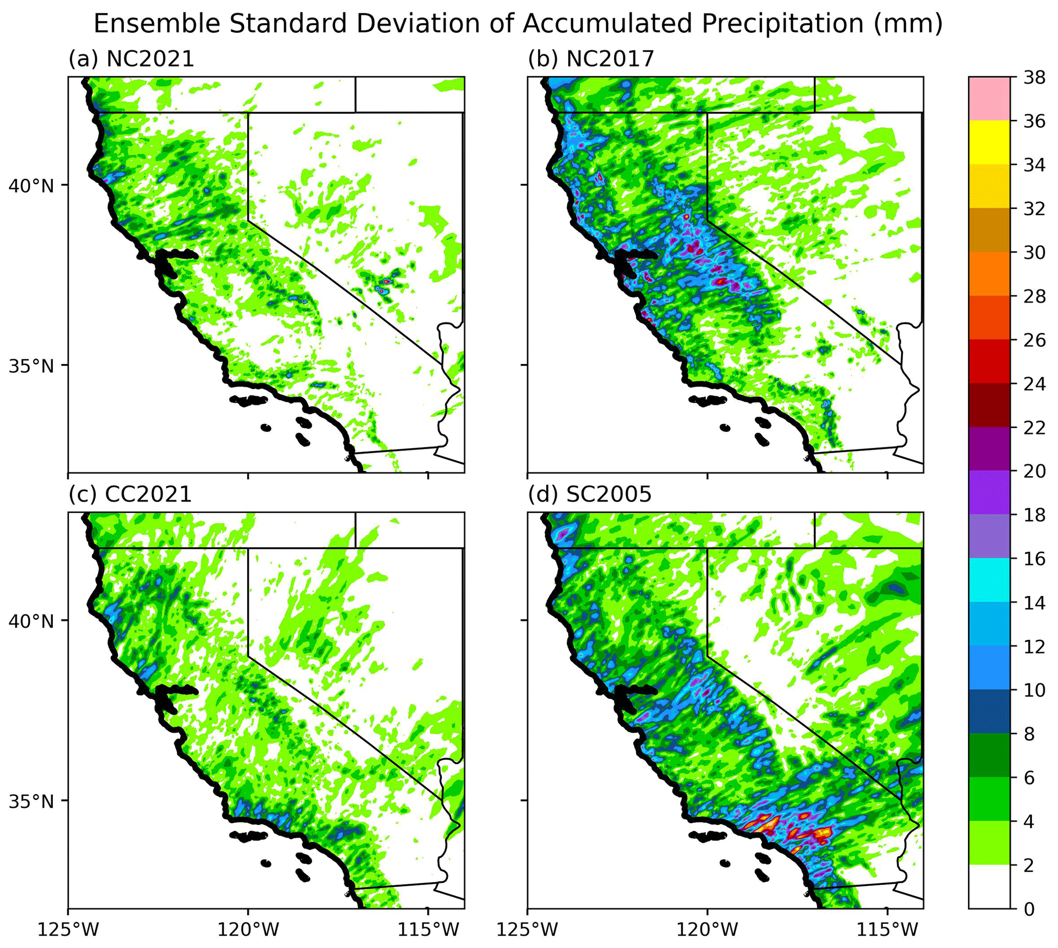
Figure 15Standard deviation of event accumulated precipitation computed from a 10-member ensemble for each case for the CA-3km grid.
While not displayed, a small five-member ensemble was performed for the GLBP-3km configuration for the CC2021 and NC2017 cases. These were the two cases in which the GLBP-3km grid demonstrated a clear advantage over the other configurations; thus a small ensemble was performed to gain confidence that these results were not due to random chance. Indeed, we found that the relatively high correlation score obtained for the CC2021 case and reduced bias in the NC2017 case were maintained in the small ensemble runs.
Finally, all experiments performed in this paper were initialized 24 h before the AR made landfall on CA. To test the sensitivity to lead time we initialized each case and configuration 6 h before and after the default initialization time. With exception of the CC2021 case, changing the initialization time did not modify the main findings of this study. For the CC2021 case we found that initializing 6 h later led to improved correlation scores for all grid configurations (with exception of the GLBP-3km case where the score was maintained) due to a more accurate placement of the precipitation maximum on the central coast rather than the Transverse Range.
This study uses the Simple Cloud-Resolving E3SM Model (SCREAM) and its application in a regionally refined mesh (RRM) configuration to simulate AR events. The research aims to assess SCREAM's ability to simulate ARs over California, examine the impact of resolution and RRM fine mesh size, and address questions regarding the fidelity of AR simulations, their improved forecast potential with higher resolution, and the significance of RRM location. The work utilizes four meteorologically distinct AR event cases and evaluates model performance against observational datasets. This approach aims to enhance our understanding of AR precipitation representation not only in SCREAM, but also in climate and weather models at large.
SCREAM effectively reproduces the magnitude and structure of AR-associated integrated vapor transport (IVT) but exhibits some discrepancies (Fig. 5). It performs well in simulating warm ARs like NC2021 but has a statewide positive precipitation bias for all cases, with challenges in representing colder ARs, particularly NC2017 (Fig. 6). Interestingly, resolution does not significantly impact precipitation or snowfall simulation. The GLBP-3km global high-resolution proxy grid configuration shows advantages in some cases. SCREAM generally exhibits a positive temperature bias (Fig. 12) and tends to overestimate precipitation in topographic areas (Fig. 8). While SCREAM captures fine-scale details and moisture flux adequately, it underrepresents maximum IVT on the leeward side of the Sierra Nevada (Figs. 13 and 14). Ensembles and sensitivity tests confirm robustness in the model's results (Fig. 15). In conclusion, SCREAM shows reasonable skill in simulating ARs, but addressing biases and improving accuracy in representing AR events and their impacts need some improvement.
The aforementioned positive precipitation bias of 10 %–33 % seen in our simulations is far less than the climatological bias produced by the CA-3km grid in Zhang et al. (2024). This suggests that a large majority of the bias produced in that work originates from errors pertaining to the large-scale forcing with smaller, though non-negligible, errors specific to SCREAM. While this work did not address the source of the SCREAM bias, we note that using a framework such as CA-3km hindcasts to perform perturbed parameter experiments would be a relatively efficient way to identify whether this bias is related to the uncertain tunable parameters in the model. Such an exercise would be helpful to improve the topographic precipitation bias that likely exists in regions outside of CA in SCREAM and would thus have positive global impacts on the model simulation.
A key finding of this work is the relative importance of resolution versus refined mesh size. Interestingly, we found no advantage when increasing the resolution from 3 km (ne1024) to 800 m (ne4096) in terms of the precipitation and snowfall skill scores related to ARs. We view this as a positive result in terms of the resolution fidelity of SCREAM, and it is consistent with SCREAM's muted resolution sensitivity of cloud processes in a doubly periodic configuration (Bogenschutz et al., 2023a). The lack of resolution sensitivity for topographically enhanced precipitation further demonstrates that SCREAM does not possess extreme resolution sensitivity in AR simulations, which is driven by either discretization error or model physics sensitivity. While this robust performance may not be generalizable to all models, we conclude that no significant benefits can be gained by increasing resolution within the kilometer scale for AR events if the model is reasonably scale-aware and insensitive. We hypothesize that benefits could potentially be realized should the resolution be increased beyond 400 m, as this is the scale where boundary layer turbulence is permitted and convection resolved (rather than permitted). However, we acknowledge the added challenge of evaluating sub-kilometer-scale models due to the lack of available high-resolution observations.
Unlike resolution, we did find that expanding the area of the refined mesh produced better skill scores in precipitation and snow. However, this was only achieved when the size of the mesh was expanded significantly to cover the entirety of the eastern Pacific Ocean. We found that a modest increase to the size of the refined mesh (similar to previous works of nested models when simulating AR events, i.e., the EPAC-3km configuration) did not produce such benefits, which are only realized if the incoming meteorology to CA is contained with the high-resolution region for the entire simulation. While improved precipitation skill scores were achieved with the GLBP-3km grid, the overall characteristics of simulated precipitation produced by that grid were similar to those of the other configurations. In addition, having a refined region as large as the one in the GLBP-3km configuration is counter to the cost-saving strategy that motivates using RRM in the first place. Thus, the CA-3km configuration represents an appropriate balance of computational cost while maintaining the scientific performance of the global simulation for a specific region. It is unclear if this conclusion would be robust for other regions of the globe where the incoming large-scale forcing may be more sensitive to the model resolution than the synoptic-scale ARs that strongly influence CA's annual precipitation.
Nonetheless, despite this modest sensitivity we found that SCREAM has a satisfactory representation of AR events in both the “global proxy” configuration and the most economical RRM. The most significant issue found is a positive precipitation bias over topography, which is likely an issue in other regions of the globe in SCREAM that warrants further investigation. Finally, future work should focus on the simulation of ARs in SCREAM in regions outside of California, either through global simulation or RRM, to encompass a broader range of ARs and meteorological conditions.
The code to run the simulations in addition to the model output used to generate the analysis in this paper can be found at https://doi.org/10.5281/zenodo.10836035 (Bogenschutz, 2024). The PRISM data can be obtained at https://prism.oregonstate.edu (PRISM Climate Group, 2022), the SNOTEL data at https://nwcc-apps.sc.egov.usda.gov/imap/ (US Department of Agriculture, 2024), the University of Arizona (UA) SWE data at https://doi.org/10.5067/0GGPB220EX6A (Broxton et al., 2019; Zeng et al., 2018), and the ERA5 product at https://doi.org/10.24381/cds.adbb2d47 (Hersbach et al., 2023).
PB created each grid configuration, performed the simulations, and led the analysis. JZ assisted in the creation of each grid configuration and participated in the analysis. QT assisted in the creation of the original CA RRM grid. PCS obtained funding for this work and assisted in the creation of the original CA RRM grid.
The contact author has declared that none of the authors has any competing interests.
Publisher's note: Copernicus Publications remains neutral with regard to jurisdictional claims made in the text, published maps, institutional affiliations, or any other geographical representation in this paper. While Copernicus Publications makes every effort to include appropriate place names, the final responsibility lies with the authors.
Work at LLNL was performed under the auspices of the US DOE by Lawrence Livermore National Laboratory under contract DE-AC52-07NA27344. IM release: LLNL-JRNL-861973.
This work is supported by the Lawrence Livermore National Laboratory (LLNL) LDRD project (22-SI-008) “Climate Resilience for National Security”.
This paper was edited by Axel Lauer and reviewed by James Benedict and one anonymous referee.
Bales, R. C., Battles, J. J., Chen, Y., Conklin, M. H., Holst, E., O’Hara, K. L., Saksa, P., and Stewart, W.: Forests and water in the Sierra Nevada: Sierra Nevada watershed ecosystem enhancement project, Sierra Nevada Research Institute report, Vol. 11, https://forests.berkeley.edu/sites/forests.berkeley.edu/files/146199.pdf (last access: 13 September 2024), 2011.
Benedict, J. J., Clement, A. C., and Medeiros, B.: Atmospheric blocking and other large-scale precursor patterns of landfalling atmospheric rivers in the North Pacific: A CESM2 study, J. Geophys. Res.-Atmos., 124, 11330–11353, https://doi.org/10.1029/2019JD030790, 2019.
Bogenschutz, P.: Code and Data for Atmospheric River Induced Precipitation in California as Simulated by the Regionally Refined Simple Convective Resolving E3SM Atmosphere Model Version 0, Zenodo [data set], https://doi.org/10.5281/zenodo.10836035, 2024.
Bogenschutz, P. and Krueger, S. K.: A simplified PDF parameterization of subgrid-scale clouds and turbulence for cloud-resolving models, J. Adv. Model. Earth Sy., 5, 195–211, https://doi.org/10.1002/jame.20018, 2013.
Bogenschutz, P. A., Yamaguchi, T., and Lee, H.-H.: The Energy Exascale Earth System Model simulations With high vertical resolution in the lower troposphere, J. Adv. Model. Earth Sy., 13, e2020MS002239, https://doi.org/10.1029/2020MS002239, 2021.
Bogenschutz, P. A., Eldred, C., and Caldwell, P. M.: Horizontal resolution sensitivity of the Simple Convection-Permitting E3SM Atmosphere Model in a doubly-periodic configuration, J. Adv. Model. Earth Sy., 15, e2022MS003466, https://doi.org/10.1029/2022MS003466, 2023a.
Bogenschutz, P. A., Lee, H.-H., Tang, Q., and Yamaguchi, T.: Combining regional mesh refinement with vertically enhanced physics to target marine stratocumulus biases as demonstrated in the Energy Exascale Earth System Model version 1, Geosci. Model Dev., 16, 335–352, https://doi.org/10.5194/gmd-16-335-2023, 2023b.
Broxton, P., Zeng, X., and Dawson, N.: Daily 4 km Gridded SWE and Snow Depth from Assimilated In-Situ and Modeled Data over the Conterminous US, Version 1, Boulder, Colorado USA, NASA National Snow and Ice Data Center Distributed Active Archive Center [data set], https://doi.org/10.5067/0GGPB220EX6A, 2019.
Caldwell, P. M., Mametjanov, A., Tang, Q., Van Roekel, L. P., Golaz, J.-C., and Lin, W.: The DOE E3SM coupled model version 1: Description and results at high resolution, J. Adv. Model. Earth Sy., 11, 4095–4146, https://doi.org/10.1029/2019MS001870, 2019.
Caldwell, P. M., Terai, C. R., Hillman, B., Keen, N. D., Bogenschutz, P., and Lin, W.: Convection-permitting simulations with the E3SM global atmosphere model, J. Adv. Model. Earth Sy., 13, e2021MS002544, https://doi.org/10.1029/2021MS002544, 2021.
Carrera, M. L., Higgins, R. W., and Kousky, V. E.: Downstream weather impacts associated with atmospheric blocking over the northeast Pacific, J. Climate, 17, 4823–4839, https://doi.org/10.1175/jcli-3237.1, 2004.
Davini, P. and D’Andrea, F.: From CMIP3 to CMIP6: Northern Hemisphere Atmospheric Blocking Simulation in Present and Future Climate, J. Climate, 33, 10021–10038, https://doi.org/10.1175/JCLI-D-19-0862.1, 2020.
Delworth, T. L., Rosati, A., Anderson, W., Adcroft, A. J., Balaji, V., Benson, R., Dixon, K., Griffies, S. M., Lee, H.-C., Pacanowski, R. C., Vecchi, G. A., Wittenberg, A. T., Zeng, F., and Zhang, R.: Simulated climate and climate change in the gfdl cm2.5 high-resolution coupled climate model, J. Climate, 25, 2755–2781, https://doi.org/10.1175/JCLI-D-11-00316.1, 2012.
Duffy, P. B., Govindasamy, B., Iorio, J. P., Milanovich, J., Sperber, K. R., Taylor, K. E., Wehner, M. F., and Thompson, S. L.: High-resolution simulations of global climate, part 1: present climate, Clim. Dynam., 21, 371–390, 2003.
Eldardiry, H., Mahmood, A., Chen, X., Hossain, F., Nijssen, B., and Lettenmaier, D. P.: Atmospheric river-induced precipitation and snowpack during the western United States cold season, J. Hydrometeorol., 20, 613–630, https://doi.org/10.1175/JHMD-18-0228.1, 2019.
Hannah, W. M., Bradley, A. M., Guba, O., Tang, Q., Golaz, J. C., and Wolfe, J.: Separating Physics and Dynamics Grids for Improved Computational Efficiency in Spectral Element Earth System Models, J. Adv. Model. Earth Sy., 13, e2020MS002419, https://doi.org/10.1029/2020MS002419, 2021.
Hersbach, H., Bell, B., and Berrisford, P: The ERA5 global reanalysis, Q. J. Roy. Meteor. Soc., 146, 1999–2049, https://doi.org/10.1002/qj.3803, 2020.
Hersbach, H., Bell, B., Berrisford, P., Biavati, G., Horányi, A., Muñoz Sabater, J., Nicolas, J., Peubey, C., Radu, R., Rozum, I., Schepers, D., Simmons, A., Soci, C., Dee, D., and Thépaut, J.-N.: ERA5 hourly data on single levels from 1940 to present. Copernicus Climate Change Service (C3S) Climate Data Store (CDS) [data set], https://doi.org/10.24381/cds.adbb2d47, 2023.
Huang, X. and Ullrich, P. A.: The changing character of 21st century precipitation over the western United States in the variable-resolution CESM, J. Climate, 30, 7555–7575, 2017.
Huang, X. and Swain, D. L.: Climate change is increasing the risk of a California megaflood, Sci. Adv., 8, eabq0995, https://doi.org/10.1126/sciadv.abq0995, 2022.
Huang, X., Hall, A. D., and Berg, N.: Anthropogenic warming impacts on today's Sierra Nevada snowpack and flood risk, Geophys. Res. Lett., 45, 6215–6222, https://doi.org/10.1029/2018gl077432, 2018.
Huang, X., Swain, D. L., Walton, D. B., Stevenson, S., and Hall, A. D.: Simulating and evaluating atmospheric river-induced precipitation extremes along the U.S. Pacific Coast: Case studies from 1980–2017, J. Geophys. Res.-Atmos., 125, e2019JD031554, https://doi.org/10. 1029/2019JD031554, 2020.
Hurrell, J. W., Holland, M. M., Gent, P. R., Ghan, S., Kay, J. E., Kushner, P. J., Lamarque, J.-F., Large, W. G., Lawrence, D., Lindsay, K., Lipscomb, W. H., Long, M. C., Mahowald, N., Marsh, D. R., Neale, R. B., Rasch, P., Vavrus, S., Vertenstein, M., Bader, D., Collins, W. D., Hack, J. J., Kiehl, J., and Marshall, S.: The Community Earth System Model: A framework for collaborative research, B. Am. Meteorol. Soc., 94, 1339–1360, https://doi.org/10.1175/BAMS-D-12-00121.1, 2013.
Lee, H.-H, Bogenschutz, P. A., and Yamaguchi, T.: The Implementation of Framework for Improvement by Vertical Enhancement into Energy Exascale Earth System Model, J. Adv. Model. Earth Sy., 13, e2020MS002240, https://doi.org/10.1029/2020MS002240, 2021.
Lee, H.-H., Bogenschutz, P. A., and Yamaguchi, T.: Resolving away stratocumulus biases in modern global climate models, Geophys. Res. Lett., 49, e2022GL099422, https://doi.org/10.1029/2022GL099422, 2022.
Leeper, R. D., Rennie, J., and Palecki, M. A.: Observational Perspectives from U.S. Climate Reference Network (USCRN) and Cooperative Observer Program (COOP) Network: Temperature and Precipitation Comparison, J. Atmos. Ocean. Tech., 32, 703–721, https://doi.org/10.1175/JTECH-D-14-00172.1, 2015.
Leung, L. R. and Qian, Y.: Atmospheric rivers induced heavy precipitation and flooding in the western U.S. simulated by the WRF regional climate model, Geophys. Res. Lett., 36, L03820, https://doi.org/10.1029/2008GL036445, 2009.
Liu, W., Ullrich, P. A., Li, J., Zarzycki, C., Caldwell, P. M., Leung, L. R., and Qian, Y.: The June 2012 North American Derecho: A Testbed for Evaluating Regional and Global Climate Modeling Systems at Cloud-Resolving Scales, J. Adv. Model. Earth Sy., 15, e2022MS003358, https://doi.org/10.1029/2022ms003358, 2023.
Lott, N., Sittel, M. C., and Ross, D.: The winter of '96-'97: West coast flooding, Vol. 97–01, 1–22, National Climatic Data Center technical report, https://repository.library.noaa.gov/view/noaa/13812 (last access: 13 September 2024), 1997.
Lundquist, J., Hughes, M., Gutmann, E., and Kapnick, S.: Our Skill in Modeling Mountain Rain and Snow is Bypassing the Skill of Our Observational Networks, B. Am. Meteorol. Soc., 100, 2473–2490, https://doi.org/10.1175/BAMS-D-19-0001.1, 2019.
Morrison, H. and Milbrandt, J. A.: Parameterization of cloud microphysics based on the prediction of the bulk ice particle properties. Part I: Scheme description and idealized tests, J. Atmos. Sci., 72, 287–311, https://doi.org/10.1175/jas-d-14-0065.1, 2015.
Pincus, R., Mlawer, E. J., and Delamere, J. S.: Balancing accuracy, efficiency, and flexibility in radiation calculations for dynamical models, J. Adv. Model. Earth Sy., 11, 3074–3089, https://doi.org/10.1029/2019MS001621, 2019.
PRISM Climate Group: Oregon State University, https://prism.oregonstate.edu, last access: 11 December 2022.
Ralph, F. M., Neiman, P. J., and Wick, G. A.: Satellite and CALJET aircraft observations of atmospheric rivers over the eastern North Pacific Ocean during the winter of 1997/98, Mon. Weather Rev., 132, 1721–1745, https://doi.org/10.1175/1520-0493(2004)1321721:SACAOO.2.0.CO;2, 2004.
Ralph, F. M., Rutz, J. J., Cordeira, J. M., Dettinger, M., Anderson, M., Reynolds, D., Schick, L. J., and Smallcomb, C.: A scale to characterize the strength and impacts of atmospheric rivers, B. Am. Meteorol. Soc., 100, 269–289, 2019.
Rhoades, A. M., Jones, A. D., O'Brien, T. A., O'Brien, J. P., Ullrich, P. A., and Zarzycki C. M.: Influences of North Pacific Ocean domain extent on the western U.S. winter hydroclimatology in variable-resolution CESM, J. Geophys. Res.-Atmos., 125, e2019JD031977, https://doi.org/10.1029/2019JD031977, 2020.
Rhoades, A. M., Zarzycki, C. M., Inda-Diaz, H. A., Ombadi, M., Pasquier, U., and Srivastava, A.: Recreating the California New Year's flood event of 1997 in a regionally refined Earth system model, J. Adv. Model. Earth Sy., 15, e2023MS003793, https://doi.org/10.1029/2023MS003793, 2023.
Ringler, T., Ju, L., and Gunzburger, M.: A multiresolution method for climate system modeling: application of spherical centroidal Voronoi tessellations, Ocean Dynam., 58, 475–498, https://doi.org/10.1007/s10236-008-0157-2, 2008.
Risser, M. D., Paciorek, C. J., Wehner, M. F., O'Brien, T. A., and Collins, W. D.: A probablistic gridded product for daily precipitation extremes over the United State, Clim. Dynam., 53, 2517–2538, https://doi.org/10.1007/s00382-019-04636-0, 2019.
Rutz, J. J., Steenburgh, W. J., and Ralph, F. M.: Climatological Characteristics of Atmospheric Rivers and Their Inland Penetration over the Western United States, Mon. Weather Rev., 142, 905–921, https://doi.org/10.1175/MWR-D-13-00168.1, 2014.
Schiemann, R., Athanasiadis, P., Barriopedro, D., Doblas-Reyes, F., Lohmann, K., Roberts, M. J., Sein, D. V., Roberts, C. D., Terray, L., and Vidale, P. L.: Northern Hemisphere blocking simulation in current climate models: evaluating progress from the Climate Model Intercomparison Project Phase 5 to 6 and sensitivity to resolution, Weather Clim. Dynam., 1, 277–292, https://doi.org/10.5194/wcd-1-277-2020, 2020.
Shields, C. A. and Kiehl, J. T.: Simulating the pineapple express in the half degree community climate system model, CCSM4, Geophys. Res. Lett., 43, 7767–7773, https://doi.org/10.1002/2016GL069476, 2016.
Stevens, B., Satoh, M., and Auger, L.: Dyamond: the dynamics of the atmospheric general circulation modeled on non-hydrostatic domains, Prog. Earth Pl. Sci., 6, 61, https://doi.org/10.1186/s40645-019-0304-z, 2019.
Swain, D. L., Langenbrunner, B., Neelin, J. D., and Hall, A.: Increasing precipitation volatility in twenty-first-century California, Nat. Clim. Change, 8, 427, https://doi.org/10.1038/s41558-018-0140-y, 2018.
Tang, Q., Klein, S. A., Xie, S., Lin, W., Golaz, J.-C., Roesler, E. L., Taylor, M. A., Rasch, P. J., Bader, D. C., Berg, L. K., Caldwell, P., Giangrande, S. E., Neale, R. B., Qian, Y., Riihimaki, L. D., Zender, C. S., Zhang, Y., and Zheng, X.: Regionally refined test bed in E3SM atmosphere model version 1 (EAMv1) and applications for high-resolution modeling, Geosci. Model Dev., 12, 2679–2706, https://doi.org/10.5194/gmd-12-2679-2019, 2019.
Tang, Q., Golaz, J.-C., Van Roekel, L. P., Taylor, M. A., Lin, W., Hillman, B. R., Ullrich, P. A., Bradley, A. M., Guba, O., Wolfe, J. D., Zhou, T., Zhang, K., Zheng, X., Zhang, Y., Zhang, M., Wu, M., Wang, H., Tao, C., Singh, B., Rhoades, A. M., Qin, Y., Li, H.-Y., Feng, Y., Zhang, Y., Zhang, C., Zender, C. S., Xie, S., Roesler, E. L., Roberts, A. F., Mametjanov, A., Maltrud, M. E., Keen, N. D., Jacob, R. L., Jablonowski, C., Hughes, O. K., Forsyth, R. M., Di Vittorio, A. V., Caldwell, P. M., Bisht, G., McCoy, R. B., Leung, L. R., and Bader, D. C.: The fully coupled regionally refined model of E3SM version 2: overview of the atmosphere, land, and river results, Geosci. Model Dev., 16, 3953–3995, https://doi.org/10.5194/gmd-16-3953-2023, 2023.
Taylor, M. A., Guba, O., Steyer, A., Ullrich, P. A., Hall, D. M., and Eldrid, C.: An Energy Consistent Discretization of the Nonhydrostatic Equations in Primitive Variables, J. Adv. Model. Earth Sy., 12, e2019MS001783, https://doi.org/10.1029/2019MS001783, 2020.
Terai, C. R., Caldwell, P. M., Klein, S. A., Tang, Q., and Branstetter, M. L.: The atmospheric hydrologic cycle in the acme v0.3 model, Clim. Dynam., 50, 3251–3279, https://doi.org/10.1007/s00382-017-3803-x, 2018.
US Department of Agriculture: Natural Resource Conservation Service, National Water and Climate Center, United States, Air and Water Database, https://nwccapps.sc.egov.usda.gov/, last access: 10 January 2024.
Wehner, M. F., Smith, R. L., Bala, G., and Duffy, P.: The effect of horizontal resolution on simulation of very extreme us precipitation events in a global atmosphere model, Clim. Dynam., 34, 241–247, https://doi.org/10.1007/s00382-009-0656-y, 2010.
Zarzycki, C. M. and Jablonowski, C.: Experimental Tropical Cyclone Forecasts Using a Variable-Resolution Global Model, Mon. Weather Rev., 143, 4012–4037, 2015.
Zeng, X., Boxton, P., and Dawson, N.: Snowpack change from 1982 to 2016 over conterminous United States, Geophys. Res. Lett., 45, 12940–12947, https://doi.org/10.1029/2018GL079621, 2018.
Zhang, J., Bogenschutz, P., Tang, Q., Cameron-smith, P., and Zhang, C.: Leveraging regional mesh refinement to simulate future climate projections for California using the Simplified Convection-Permitting E3SM Atmosphere Model Version 0, Geosci. Model Dev., 17, 3687–3731, https://doi.org/10.5194/gmd-17-3687-2024, 2024.
Zhou, Y. and Kim, H.: Impact of Distinct Origin Locations on the Life Cycles of Landfalling Atmospheric Rivers Over the U.S. West Coast, J. Geophys. Res.-Atmos., 124, 11897–11909, https://doi.org/10.1029/2019JD031218, 2019.