Southern Ocean Ice Prediction System version 1.0 (SOIPS v1.0): description of the system and evaluation of synoptic-scale sea ice forecasts

An operational synoptic-scale sea ice forecasting system for the Southern Ocean, namely the Southern Ocean Ice Prediction System (SOIPS), has been developed to support ship navigation in the Antarctic sea ice zone. Practical application of the SOIPS forecasts had been implemented for the 38th Chinese National Antarctic Research Expedition for the first time. The SOIPS is configured on an Antarctic regional sea ice–ocean–ice shelf coupled model and an ensemble-based localized error subspace transform Kalman filter data assimilation model. Daily near-real-time satellite sea ice concentration observations are assimilated into the SOIPS to update sea ice concentration and thickness in the 12 ensemble members of the model state. By evaluating the SOIPS performance in forecasting sea ice metrics in a complete melt–freeze cycle from 1 October 2021 to 30 September 2022, this study shows that the SOIPS can provide reliable Antarctic sea ice forecasts. In comparison with non-assimilated EUMETSAT Ocean and Sea Ice Satellite Application Facility (OSI SAF) data, annual mean root mean square errors in the sea ice concentration forecasts at a lead time of up to 168 h are lower than 0.19, and the integrated ice edge errors in the sea ice forecasts in most freezing months at lead times of 24 and 72 h maintain around 0.5×10⁶ km² and below 1.0×10⁶ km², respectively. With respect to the scarce Ice, Cloud, and land Elevation Satellite-2 (ICESat-2) observations, the mean absolute errors in the sea ice thickness forecasts at a lead time of 24 h are lower than 0.3 m, which is in the range of the ICESat-2 uncertainties. Specifically, the SOIPS has the ability to forecast sea ice drift, in both magnitude and direction. The derived sea ice convergence rate forecasts have great potential for supporting ship navigation on a fine local scale. The comparison between the persistence forecasts and the SOIPS forecasts with and without data assimilation further shows that both model physics and the data assimilation scheme play important roles in producing reliable sea ice forecasts in the Southern Ocean.

1 Introduction

Surrounding Antarctica, sea ice motion in the Southern Ocean is fast. This situation is partly caused by the natural feature of Antarctic sea ice, where the majority of the ice is thin first-year ice. Wind force leads to faster ice speed if ice thickness is thinner. Moreover, the severe Antarctic environmental conditions, such as frequent westerly cyclones, a complicated surface ocean circulation system, and drastic nighttime katabatic winds off the ice shelf and coast, also promote the rapid ice motion. Beyond the Antarctic Peninsula, the topographic shape of the high-latitude Southern Ocean without a land barrier in the zonal direction provides an advantage for rapid sea ice movement (Worby et al., 1998; Heil and Allison, 1999; Turner et al., 2002; Wang et al., 2014; Womack et al., 2022). Energetic sea ice in the Southern Ocean has become one of the major challenges for safe maritime navigation due to the lack of timely and accurate sea ice forecasting information (Wagner et al., 2020); e.g., during the austral summer of 2013–2014, both the Russian icebreaker MV Akademik Shokalskiy and the Chinese icebreaker MV Xue Long were trapped in the Adélie Depression region by quickly convergent sea ice under the influence of several cyclones (Witze, 2014; Turney, 2014; Zhai et al., 2015). Earlier in November 2007, the cruise ship MS Explorer sunk between the South Shetland Islands and Graham Land in the Bransfield Strait, after striking an iceberg near the South Shetland Islands, an area which is usually stormy but was calm at the time. Hence, reliable synoptic Antarctic sea ice forecasts are of great importance to Antarctic maritime commercial and scientific activities in the coming decades, when human activities in the Southern Ocean are expected to flourish.

However, partly owing to the relatively small number of people who need Antarctic sea ice information, few attempts have been made by international weather forecasting centers to construct an operational synoptic-scale sea ice forecasting system for the Southern Ocean in comparison to the multiple kinds of Arctic sea ice forecasting systems. The Canadian Meteorological Centre (CMC) operates the Global Ice Ocean Prediction System (GIOPS; Smith et al., 2016), which is built on the Nucleus for European Modelling of the Ocean (NEMO) version 3.1 and the Los Alamos National Laboratory Community Ice CodE (CICE) version 4.0, and the system is driven by atmospheric forcing from the Global Deterministic Prediction System. Since 2011, GIOPS has been providing 10 d forecasts of global ocean and sea ice, including the Southern Ocean, at a resolution of 0.25°. The United Kingdom Met Office (UKMO) operates the Forecast Ocean Assimilation Model (FOAM; Blockley et al., 2014), which is also based on NEMO and CICE. Driven by atmospheric variables at the ocean surface from the Met Office Unified Model (UM) global numerical weather prediction (NWP) system, FOAM produces 7 d forecasts of global ocean tracers, ocean currents, and polar sea ice with a horizontal resolution of 0.25°. Under the framework of the Copernicus Marine Environment Monitoring Service (CMEMS), the Mercator Ocean International (MOI) has developed a global ocean real-time monitoring and $\mathrm{1}/\mathrm{12}$° high-resolution forecasting system (GLO-HR; Lellouche et al., 2018) based on NEMO and the Louvain-la-Neuve Sea Ice Model version 2 (LIM2), and the atmospheric forcing is taken from the Integrated Forecasting System (IFS). GLO-HR delivers 10 d forecasts for the global ocean and polar sea ice on a daily basis. The US Navy's Global Ocean Forecast System version 3.1 (GOFS 3.1) is based on the HYbrid Coordinate Ocean Model (HYCOM) and CICE and provides a global sea ice prediction capability including both the Arctic and the Antarctic (Posey et al., 2015). SEAS5, the fifth-generation seasonal forecast system of the European Centre for Medium-Range Weather Forecasts (ECMWF), which constitutes the NEMO ocean model, LIM2 sea ice model, and IFS atmospheric model, has a horizontal resolution of 0.25° for the global ocean and sea ice and provides 10 d forecasts of Antarctic sea ice cover and snow depth (Johnson et al., 2019). Nevertheless, all the above-mentioned operational forecasting systems are built on global coupled models, and their focus is not purely on Antarctic sea ice forecasts. Although the resolution of global models is constantly becoming finer, regional ice–ocean coupled models at a similar resolution but with lower computational cost still offer some advantages when appropriate initial and boundary conditions are adopted (Mu et al., 2019; Liang et al., 2020; Ren et al., 2021).

Data assimilation is an essential way to reduce short-term forecast uncertainties by providing an optimally estimated initial state, which has long been employed in geophysical or biogeochemical applications (Verdy and Mazloff, 2017). Various data assimilation algorithms have been widely used to assimilate multi-source observations into sea ice forecasting and analysis systems (Lindsay and Zhang, 2006; Massonnet et al., 2013; Luo et al., 2021). Both GIOPS and GLO-HR use the System Assimilation Mercator version 2 (SAM2) as their ocean assimilation system, which was developed from the singular evolutive extended Kalman (SEEK) algorithm (Tranchant et al., 2006). FOAM and SEAS5 adopt a 3D-Var data assimilation system for use with NEMO, namely NEMOVAR (Mignac et al., 2022; Mogensen et al., 2009, 2012). GOFS 3.1 employs the Navy Coupled Ocean Data Assimilation (NCODA) system based on the 3D-Var method (Cummings and Smedstad, 2014). The Southern Ocean State Estimate (Mazloff et al., 2010) constrains the model state using in situ and satellite measurements through 4D-Var data assimilation. These systems mainly assimilate near-real-time satellite observations of sea ice concentration, sea level anomaly, and sea surface temperature together with in situ observations of ocean temperature and salinity profiles. Previous studies have shown that the ensemble Kalman filter (EnKF) algorithm using dynamic background error covariance is suitable for multi-variable data assimilation in polar regions because it does not need to develop complex adjoint models and is computationally efficient; it has thus been widely used in Arctic sea ice forecasts (Sakov et al., 2012; Yang et al., 2014, 2015, 2016; Mu et al., 2018; Liang et al., 2019).

In order to address the pressing need for sea ice forecasts in the Southern Ocean, especially in support of the Chinese National Antarctic Research Expedition (CHINARE), the motivation of this work is to describe a newly developed regional synoptic-scale forecasting system for Antarctic sea ice, i.e., the Southern Ocean Ice Prediction System version 1.0 (SOIPS v1.0), which is based on a sea ice–ocean–ice shelf coupled model and an EnKF data assimilation algorithm. The SOIPS has been operational since 1 January 2021 and provided sea ice forecasts for the 38th CHINARE-Antarctic during the austral summer of 2021–2022. By evaluating sea ice forecasts in a complete melt–freeze cycle between 1 October 2021 and 30 September 2022, we show in this study that this new system has the ability to provide precise forecasts for Antarctic sea ice evolution at a synoptic timescale, where the forecast accuracy of sea ice drift in particular is substantially guaranteed. The paper is organized as follows. In Sect. 2, the system configuration, data assimilation strategy, and design of comparison experiments are described in detail. Antarctic sea ice forecasts, including the sea ice concentration, sea ice edge, sea ice thickness, sea ice drift, and sea ice convergence rate, are evaluated in Sect. 3. Conclusions and discussions are presented in Sect. 4.

2 System description

2.1 Model configuration

The regional sea ice–ocean–ice shelf coupled model of the SOIPS is configured on the Massachusetts Institute of Technology general circulation model (MITgcm; Marshall et al., 1997; Losch et al., 2010). The ocean model uses curvilinear coordinates with the open boundaries far north, away from the domain of the Antarctic Circumpolar Current (ACC) and any likely northern extent of the sea ice. There are 496×496 grid points in horizontal with an average resolution of ∼18 km (Fig. 1). Vertically, it is composed of 50 unevenly spaced layers with intervals from 10 m near the surface to 450 m at the bottom. The ocean model utilizing the finite-volume incompressible Navier–Stokes equations adopts the bulk formula for heat and momentum calculations at the surface (Large and Pond, 1981, 1982) and the K-profile parameterization (KPP) for vertical mixing in the ocean interior (Large et al., 1994). The viscous-plastic rheology (Hibler, 1979; Zhang and Hibler, 1997) and the zero-layer ice/snow thermodynamics (Semtner, 1976) are used in the sea ice model, which shares the same horizontal mesh with the ocean model. The ice shelf, serving as a static surface boundary condition, exerts dynamic and thermodynamic influences on the underlying ocean and thus affects ocean circulation and sea ice (Losch, 2008). Dynamically, the ice shelf draft on the top of the water column has a similar role to the surface orography. Underneath an ice shelf, the pressure at the top of the water column is the sum of the atmospheric pressure and the weight of the ice shelf column. Thermodynamically, the freezing and melting at the basal surface of the ice shelf can induce an effective heat flux and a virtual salt flux at the ice–ocean interface, with an additional tendency term of temperature and salinity to the ocean at the depth of the ice shelf draft. An oceanic boundary layer underneath the ice shelf–ocean interface is formed following three physical constraints: the interface must be at the freezing point, and both heat and salt must be conserved at the interface (Holland and Jenkins, 1999). Specific landfast ice parameterization, iceberg parameterization, and tide forcing have not been included in the SOIPS. The time step of the coupled model is 1200 s.

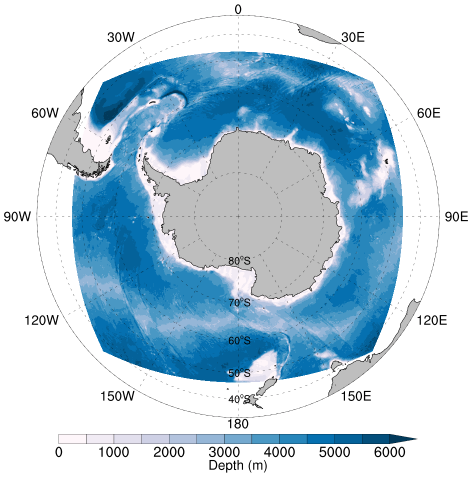
Figure 1 The domain of the Southern Ocean Ice Prediction System (SOIPS). The contours show the bathymetry in meters.

The initial fields of ocean temperature and salinity are derived from the World Ocean Atlas 2009 (WOA09; Locarnini et al., 2010; Antonov et al., 2010). The initial fields of sea ice concentration and thickness are obtained from observations of the Advanced Microwave Scanning Radiometer for the Earth Observing System (AMSR-E; Toudal Pedersen et al., 2017) and the Ice, Cloud, and land Elevation Satellite (ICESat; Kurtz and Markus, 2012), respectively. The ice shelf draft is obtained from a consistent data set of Antarctic ice sheet topography, cavity geometry, and global bathymetry (Timmermann et al., 2010). Climatological monthly mean oceanic boundary conditions are provided by the Estimating the Circulation and Climate of the Ocean phase II (ECCO2; Menemenlis et al., 2008) project, including ocean potential temperature, salinity, and velocity.

In our previous work, a model free run from 1979 to 2020 without data assimilation was successfully conducted. It was forced by atmospheric variables at the ocean surface derived from the Japanese 55-year Reanalysis (JRA55; Kobayashi et al., 2015; Harada et al., 2016), including 2 m air temperature and humidity, 10 m wind velocity components, downward shortwave and longwave radiation at the sea surface, and total precipitation. Validation of the model free run results, including the simulated sea ice extent, sea ice concentration, sea ice thickness, and net eastward oceanic volume transport across the Drake Passage, has demonstrated that this regional sea ice–ocean–ice shelf coupled model is capable of capturing the main features of Antarctic sea ice and ocean (Zhao et al., 2023).

2.2 Data assimilation scheme

The data assimilation algorithm used in the SOIPS is the ensemble-based localized error subspace transform Kalman filter (LESTKF; Nerger et al., 2012), which is packaged in the Parallel Data Assimilation Framework (PDAF; Nerger and Hiller, 2013). LESTKF is a localized variant of the error subspace transform Kalman filter (ESTKF), in which the dynamic background error covariance is applied. An optimal localization scheme that allows for an adaptive localization radius based on observation number is achieved by setting the effective local observation dimension equal to the ensemble size (Kirchgessner et al., 2014). Weights of observations within the optimal localization radius are calculated based on a fifth-order polynomial function according to the distance between the observation location and analysis grid point (Hunt et al., 2007; Gaspari and Cohn, 1999). Studies have indicated that LESTKF is suitable for high-dimensional models with small-scale local features and a large number of observations (Vetra-Carvalho et al., 2018). Considering the balance between computational efficiency and forecasting skills, 12 ensemble members are selected for the SOIPS ensemble forecasts.

The SOIPS started running operationally on 1 January 2021. The initial ensemble of the SOIPS was generated by disturbing the latest state of the model free run including sea ice concentration and thickness. The 12 perturbations which were used to initialize the SOIPS ensemble were created by applying a second-order sampling scheme (Pham, 2001) to the leading 11 EOF modes of the daily model state evolution in the historical model free run between 1 January 2019 and 31 December 2020. During each assimilation step, near-real-time 6.25 km resolution sea ice concentration data retrieved from the Advanced Microwave Scanning Radiometer 2 (AMSR2) brightness temperature data were assimilated into the SOIPS and used to update sea ice concentration and thickness in the 12 ensemble initial fields on a daily basis. Since the uncertainties in the AMSR2 observations are not the same for different sea ice concentration ranges (Spreen et al., 2008), for simplicity a uniform value of 0.15 was assigned as the representative observation error. Specifically, a post-assimilation procedure, during which the modeled sea surface salinity was adjusted according to the formula described by Liang et al. (2019) to match with the change in sea ice thickness, was carried out. Atmospheric forcing for operational forecasts were taken from the National Centers for Environmental Prediction (NCEP) Global Forecast System (GFS) 168 h atmospheric forecasts. During each forecasting step, the 12 ensemble members, after assimilating observed sea ice concentration, were separately integrated for 168 h to create 12 members of 7 d forecasts, and their ensemble mean was saved. The ensemble fields of the 24 h forecasts were also recorded as initial fields for the operational forecasts the following day (Fig. 2). In this study, we perform three experiments utilizing the SOIPS on a daily basis to disentangle the impact of data assimilation from that of model physics on the sea ice forecasts. The forecast experiment with data assimilation, denoted by DA_Forecast, assimilates the AMSR2 sea ice concentration data and is driven by the GFS data for 168 h. The forecast experiment without data assimilation, denoted by NoDA_Forecast, is driven by the GFS data for 168 h without any data assimilation. The persistence forecast experiment, denoted by PE_Forecast, uses the daily initial condition of the DA_Forecast run as forecasts of the following 168 h. The operational SOIPS actually uses the setting of the DA_Forecast run; thus sea ice forecasts of the DA_Forecast run are derived from the operational record of the SOIPS. The NoDA_Forecast and PE_Forecast runs have been conducted for comparison from 1 October 2021 to 30 September 2022.

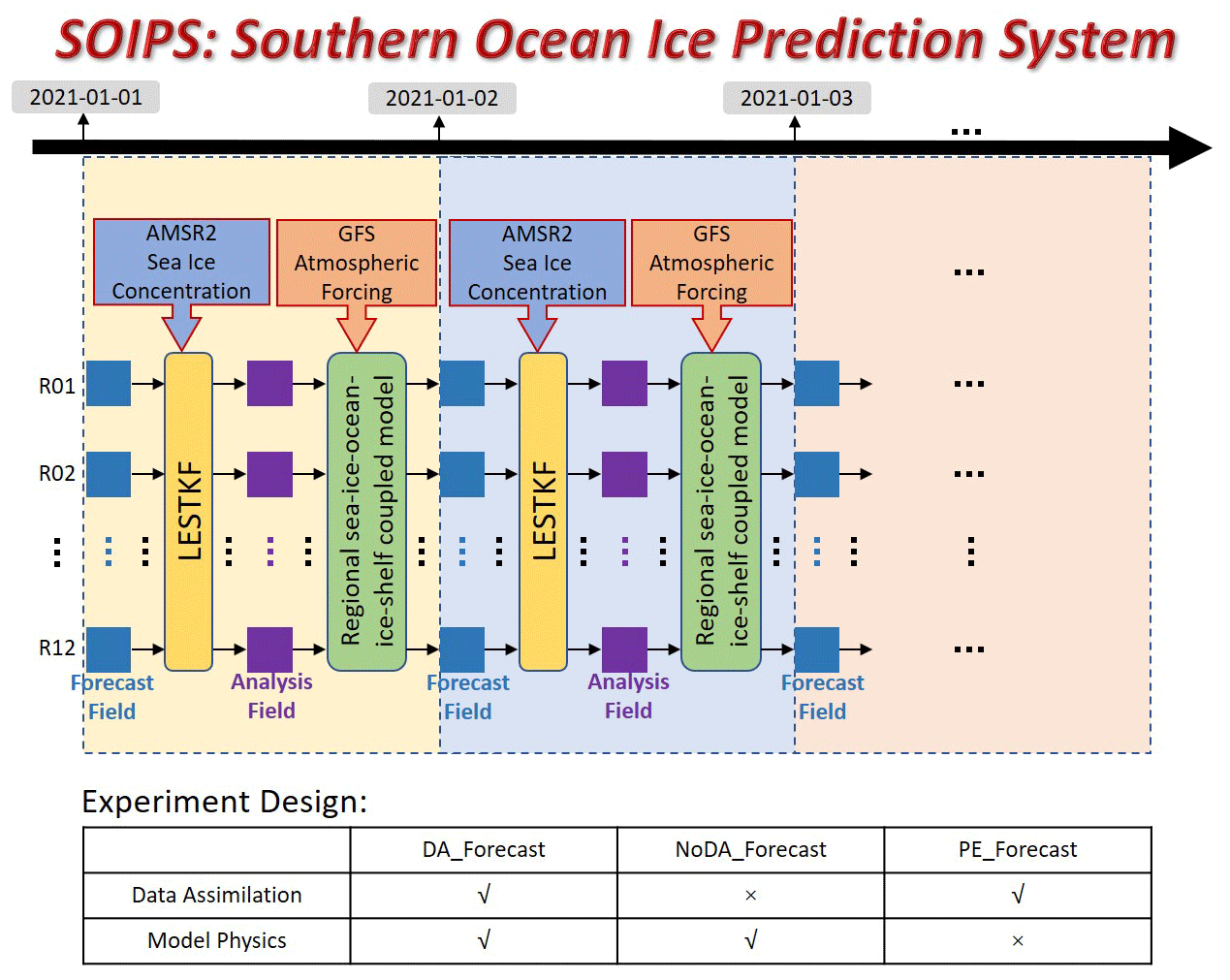
Figure 2 Schematic diagram of the SOIPS and the experiment design. The blue and purple squares denote the 12 ensemble members of the model state pre- and post-data assimilation step. The yellow block denotes the data assimilation model utilizing the ensemble-based LESTKF. The green block denotes the Antarctic regional sea ice–ocean–ice shelf coupled model. The blue block with the thick arrow denotes the near-real-time AMSR2 sea ice concentration observation. The orange block with the thick arrow denotes the operational GFS atmospheric forcing.

3 Evaluation of sea ice forecasts

The SOIPS provided forecasts of the sea ice concentration, sea ice thickness, sea ice drift, and sea ice convergence rate for the 38th CHINARE-Antarctic during the austral summer of 2021–2022. Here, we evaluate the three experiments during a complete melt–freeze cycle from 1 October 2021 to 30 September 2022. Additionally, in the Supplement, we also evaluate the operational records of the SOIPS until September 2023 to show that the SOIPS successfully predicted the historical Antarctic sea ice extent minima in 2023, and we compare the SOIPS forecasts to the physical analysis field of the Antarctic ocean produced by MOI.

3.1 Sea ice concentration

The sea ice concentration product of the EUMETSAT Ocean and Sea Ice Satellite Application Facility (OSI SAF), delivered daily at 10 km resolution in a polar stereographic projection, is used as an independent observation to evaluate the sea ice concentration forecasts. This product is computed from atmosphere-corrected brightness temperatures of the Special Sensor Microwave Imager/Sounder (SSMIS), using a combination of state-of-the-art algorithms which are different from the ARTIST Sea Ice (ASI; Spreen et al., 2008) algorithm used for AMSR2 sea ice concentration.

We calculate the root mean square errors (RMSEs) of the SOIPS forecasts at different lead times and the OSI SAF sea ice concentration observations to evaluate the performance of the SOIPS in sea ice concentration forecasts (Fig. 3). As the spatial resolution of the SOIPS is coarser than that of the OSI SAF data, we interpolate the OSI SAF data onto the model grid of the SOIPS. Basically, the RMSEs of the DA_Forecast run at each lead time gradually increase during October–March (hereafter, the latter month is used in expressions where the latter month precedes the former month to denote the month of the next year) followed by a decrease starting from April. The RMSEs of the DA_Forecast run are generally lower than 0.15 during June–September, while they are close to 0.2 during January–February. The RMSEs of the DA_Forecast run have two peaks, one in December and the other in April. The maximum RMSE of the DA_Forecast run in April is lower than 0.33. Comparison of the DA_Forecast run at different lead times shows that the RMSEs generally increase along with the prolongment of forecast lead time. Statistical analysis reveals that the annual mean RMSEs of the DA_Forecast run at lead times of 24, 72, 120, and 168 h are 0.15, 0.16, 0.17, and 0.19, respectively. Comparison of the three experiments shows that the DA_Forecast run performs the best and the NoDA_Forecast run performs the worst in most months except during late March–early June. Since the PE_Forecast run includes observed sea ice concentration information, the PE_Forecast run generally performs better than the NoDA_Forecast run and worse than the DA_Forecast run. During late March–early June, the PE_Forecast run performs worse than the other two runs at a lead time of 168 h, suggesting that sea ice changes rapidly in response to the oceanic and atmospheric forcing during this onset-to-rapid-freezing period. We also assess the difference between the assimilated AMSR2 and the OSI SAF sea ice concentration data. Due to different remote sensors and retrieval algorithms, there are significant systematic deviations between the OSI SAF and AMSR2 products. The RMSEs of these two products increase in the melting season, reaching a maximum value of 0.24 in February; thereafter the RMSEs decrease rapidly in April, maintaining below 0.15 in the rest of the freezing season. The systematic bias between the assimilated data and the validation data partly explains the sea ice concentration forecasting errors.

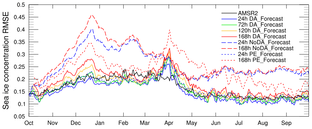
Figure 3 Time series of the RMSEs of the assimilated AMSR2 data and sea ice concentration forecasts at different lead times with respect to the OSI SAF data. The solid blue, green, yellow, red, and black lines denote the sea ice concentration forecasts of the DA_Forecast run at lead times of 24, 72, 120, and 168 h and the AMSR2 data, respectively. The long-dashed blue and red lines denote the sea ice concentration forecasts of the NoDA_Forecast run at lead times of 24 and 168 h, respectively. The short-dashed blue and red lines denote the sea ice concentration forecasts of the PE_Forecast run at lead times of 24 and 168 h, respectively.

We further analyze spatial distributions of sea ice concentration forecasting errors by evaluating monthly mean fields of the DA_Forecast run at a lead time of 24 h (Fig. 4). During October–November, relatively large RMSEs of sea ice concentration forecasts are mainly located in the north marginal ice zone surrounding Antarctica, where the sea ice, normally with a relatively low concentration and thickness, moves actively in response to external forces. In December, the RMSEs of sea ice concentration forecasts in the marginal ice zone greatly shrink, except those in the southern Atlantic Ocean sector between 30° W and 30° E. During January–February, the sea ice concentration forecasting errors are small in the entire ice zone except in some nearshore areas of the eastern Antarctic. The sea ice concentration forecasting errors start to increase in the Ross–Amundsen seas along with the northward expansion of the sea ice zone during March–April. In the following freezing months, relatively large RMSEs of sea ice concentration forecasts re-emerge in the north marginal ice zone, but their amplitudes are lower than those in the previous October–November. The monthly patterns of the RMSEs between the AMSR2 and OSI SAF data (Fig. S1 in the Supplement) resemble and lay the basis for those between the DA_Forecast run and OSI SAF data.

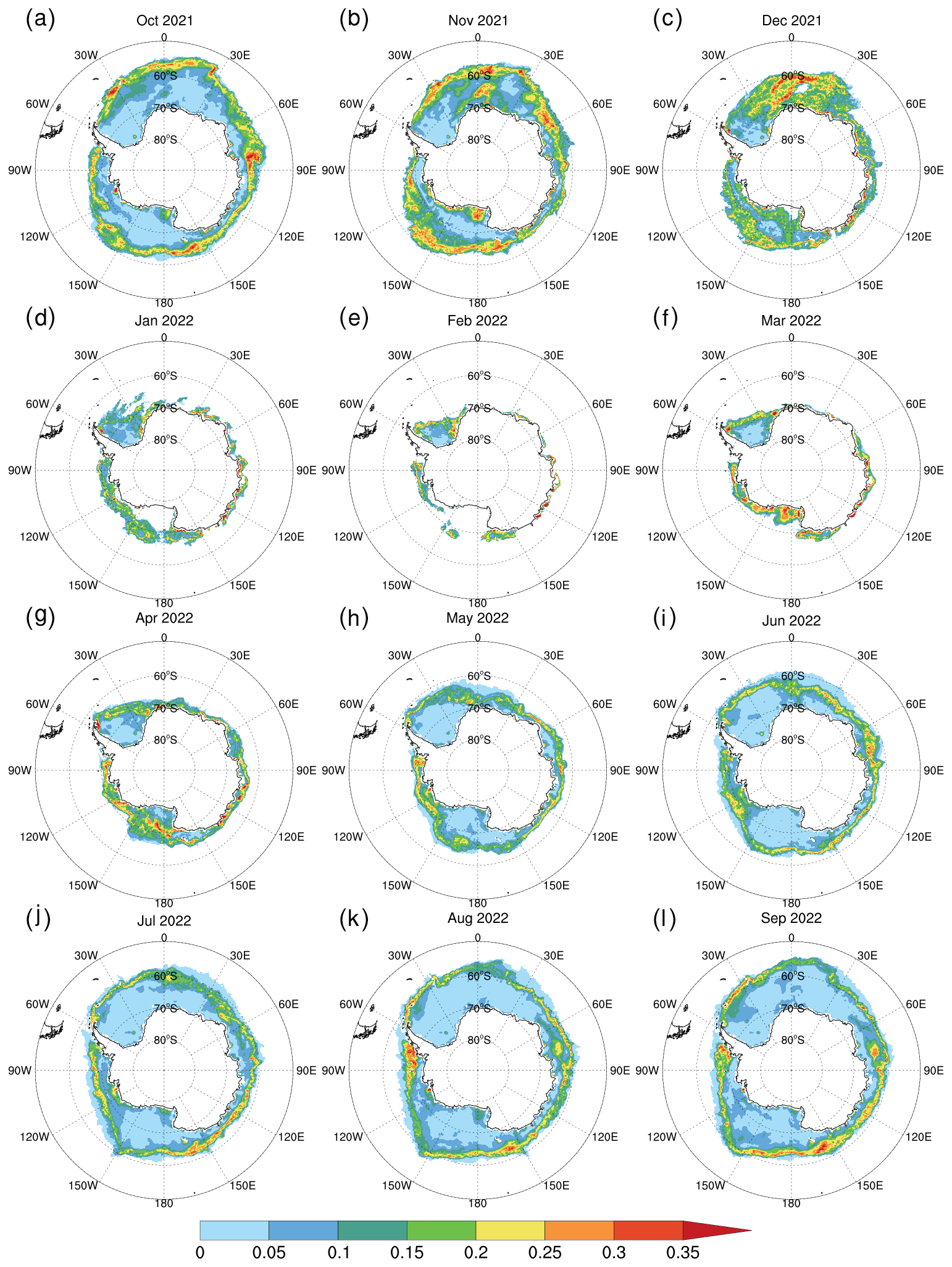
Figure 4 Monthly patterns of the sea ice concentration RMSEs of the DA_Forecast run at a lead time of 24 h with respect to the OSI SAF data. Panels (a)–(l) denote October 2021–September 2022.

3.2 Sea ice edge

Instead of evaluating just a sea ice extent number, Goessling et al. (2016) introduced a more useful verification metric, i.e., the integrated ice edge error (IIEE), which is the sum of all areas where the local sea ice extent is overestimated or underestimated. Here, the sea ice edge is defined as the locations where the sea ice concentration is 15 %. Firstly, we evaluate the derived sea ice edges from the assimilated AMSR2 and the OSI SAF data (Fig. 5). The IIEEs are larger than 0.5×10⁶ km² during October–early January and smaller than 0.5×10⁶ km² in other months. The maximum IIEE occurs in December with a value of 1.45×10⁶ km². The sea ice edge biases between the assimilated AMSR2 and the OSI SAF data contribute to the first peak in the sea ice concentration RMSEs of the DA_Forecast run in December, as shown in Fig. 3.

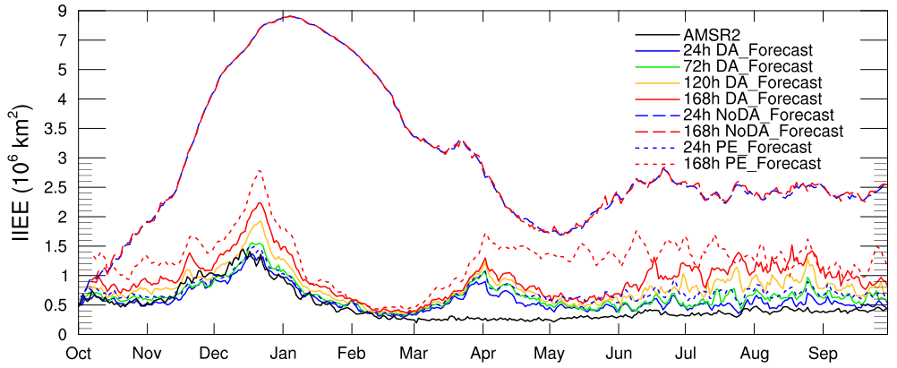
Figure 5 Time series of the IIEEs of the assimilated AMSR2 data and the forecasts at different lead times with respect to the OSI SAF data. The solid blue, green, yellow, red, and black lines denote the IIEEs of the DA_Forecast run at lead times of 24, 72, 120, and 168 h and the AMSR2 data, respectively. The long-dashed blue and red lines denote the IIEEs of the NoDA_Forecast run at lead times of 24 and 168 h, respectively. The short-dashed blue and red lines denote the IIEEs of the PE_Forecast run at lead times of 24 and 168 h, respectively.

The evolutions of the IIEEs of the DA_Forecast run at different lead times have similar shapes to those of the assimilated AMSR2 data. In December the maximum IIEEs of the DA_Forecast run at different lead times range from 1.35×10⁶ to 2.25×10⁶ km². In the early freezing season, large IIEEs of the DA_Forecast run re-emerge at the end of March, corresponding to the second peak in the sea ice concentration RMSEs of the DA_Forecast run (Fig. 3). The large IIEEs of the DA_Forecast run in late March and early April can not be attributed to the sea ice edge biases between the assimilated AMSR2 and the OSI SAF data but rather to the model's ability to accurately simulate the expansion of sea ice cover in the early freezing season. During June–September, the IIEEs of the DA_Forecast run at a lead time of 24 h maintain around 0.5×10⁶ km², and those of 72 h are below 1×10⁶ km². Comparison of the three experiments on sea ice edge forecasts shows that the DA_Forecast run performs the best, and the NoDA_Forecast run performs the worst over the whole study period.

Spatially at first glance, the sea ice edge forecasts of the DA_Forecast run at a lead time of 24 h are generally coincident with those in the OSI SAF data (Fig. 6). The sea ice edge forecasting biases of the DA_Forecast run at a lead time of 168 h (Fig. S2 in the Supplement) increase noticeably in November–December, March–April, and July–August. The areas with large sea ice edge biases are located in the southeastern Atlantic Ocean sector, southwestern Indian Ocean sector, and southwestern Pacific Ocean sector. It is noteworthy that besides the contributor to the IIEEs from the north marginal ice zone, a significant contributor to the IIEEs is from the nearshore areas surrounding Antarctica in all months. By carefully checking the coastlines or ice shelf fronts of Antarctica in the model domain and in the OSI SAF data, we realize that part of the mismatch in sea ice edges in the nearshore areas is misleading, originating from the divergence of coastlines or ice shelf fronts in the model domain and in the OSI SAF data. The lack of specific landfast ice parameterization may lead to unrealistic landfast ice zones around Antarctica, which possibly also contribute to the mismatch in sea ice edges. The real IIEEs between sea ice forecasts and the OSI SAF data should be lower than those in Fig. 5.

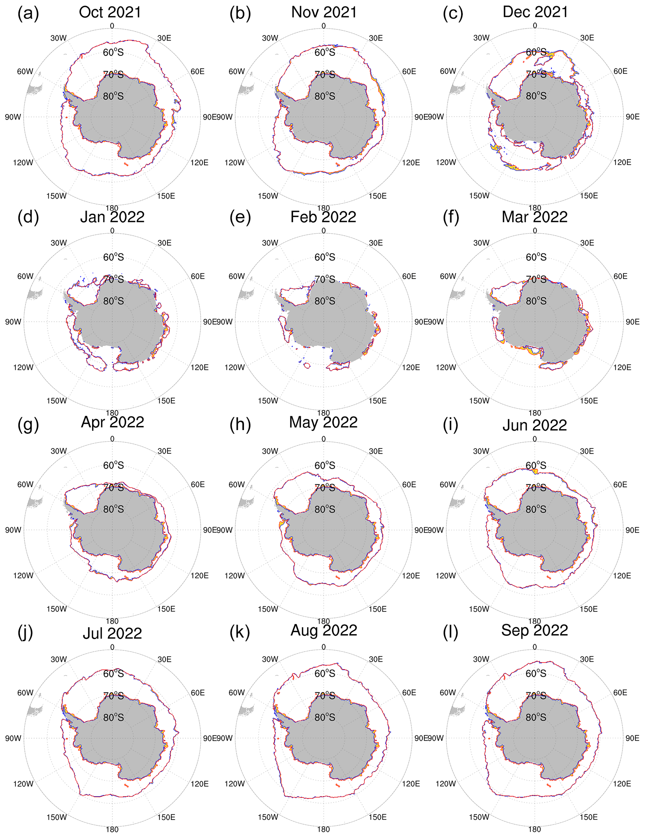
Figure 6 Monthly patterns of sea ice edge forecasts at a lead time of 24 h with respect to the OSI SAF data. Panels (a)–(l) denote October 2021–September 2022. The blue lines denote the DA_Forecast run. The red lines denote the OSI SAF data. The gold contours denote the mismatch between these two data.

3.3 Sea ice thickness

At present, continuous observations of the Antarctic sea ice thickness over a large area are still difficult to obtain. With the launch of the Ice, Cloud, and land Elevation Satellite-2 (ICESat-2) on 15 September 2018, the Antarctic sea ice freeboard can be estimated from measurements of the Advanced Topographic Laser Altimeter System (ATLAS) instrument. By applying the improved one-layer method (OLMi; Xu et al., 2021) to the daily gridded sea ice freeboard estimate product ATLAS–ICESat-2 L3B, we obtain daily Antarctic sea ice thickness distribution at discrete locations from 1 October 2021 to 30 September 2022.

We validate the daily evolution of the mean sea ice thickness forecasts at the discrete locations where observations on the corresponding date are available (Fig. 7). The results show that sea ice thickness forecasts of the DA_Forecast run at a lead time of 24 h are generally consistent with the ICESat-2 observations, with an overestimation during October–November. During most times of the validation period, the mean absolute errors (MAEs) of the sea ice thickness forecasts are lower than 0.3 m, which is significantly smaller than the uncertainties in the ICESat-2 observations. However, without assimilation of sea ice thickness data, the DA_Forecast run also performs better than the NoDA_Forecast run with respect to sea ice thickness forecasts. Sea ice thickness forecasts of the PE_Forecast run (not shown) are approximately equal to those of the DA_Forecast run at a lead time of 24 h since sea ice thickness changes by a relatively small amount in 1 d.

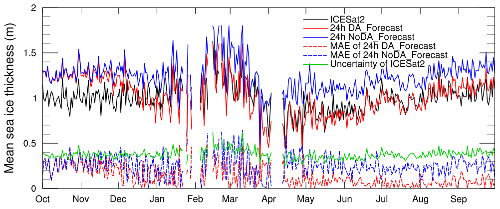
Figure 7 Time series of the mean sea ice thickness and uncertainties in the ICESat-2 observations (black and green lines), the sea ice thickness forecasts at a lead time of 24 h in the DA_Forecast and NoDA_Forecast runs (solid red and blue lines), and the mean absolute errors between the forecasts and observations (dashed red and blue lines).

We further evaluate spatial patterns of sea ice thickness forecasts of the DA_Forecast run at a lead time of 24 h (Fig. 8) after merging the daily sea ice thickness observations into seasonal mean fields. The sea ice thickness forecasts show good agreement with the observations, featured by thick ice located in the Weddell Sea, the Amundsen Sea, and the nearshore areas of the eastern Antarctic. During January–March, the DA_Forecast run overestimates ice thickness in the southern Weddell Sea, while it underestimates ice thickness in the eastern Amundsen Sea. In other seasons, the DA_Forecast run overestimates ice thickness in the western Ross Sea and the southern Weddell Sea, while it underestimates ice thickness in the Amundsen Sea and the nearshore areas of the eastern Antarctic. The forecasting errors in the southern Weddell Sea are in the range of the ICESat-2 uncertainties, but the forecasting errors in the western Ross Sea are out of the range of the ICESat-2 uncertainties. We suspect that the larger sea ice thickness biases in these areas are caused by the poor simulation of the growth rate of sea ice thickness during the freezing seasons, partly originating from the biases in the simulated ocean temperature or air temperature in the GFS data. The biases in sea ice thickness forecasts of the DA_Forecast run at a lead time of 168 h (Fig. S3 in the Supplement) do not change notably in comparison with those of 24 h. Admittedly, the above evaluation ignores the errors caused by the spatiotemporal discontinuity and the uncertainties in the ICESat-2 observations.

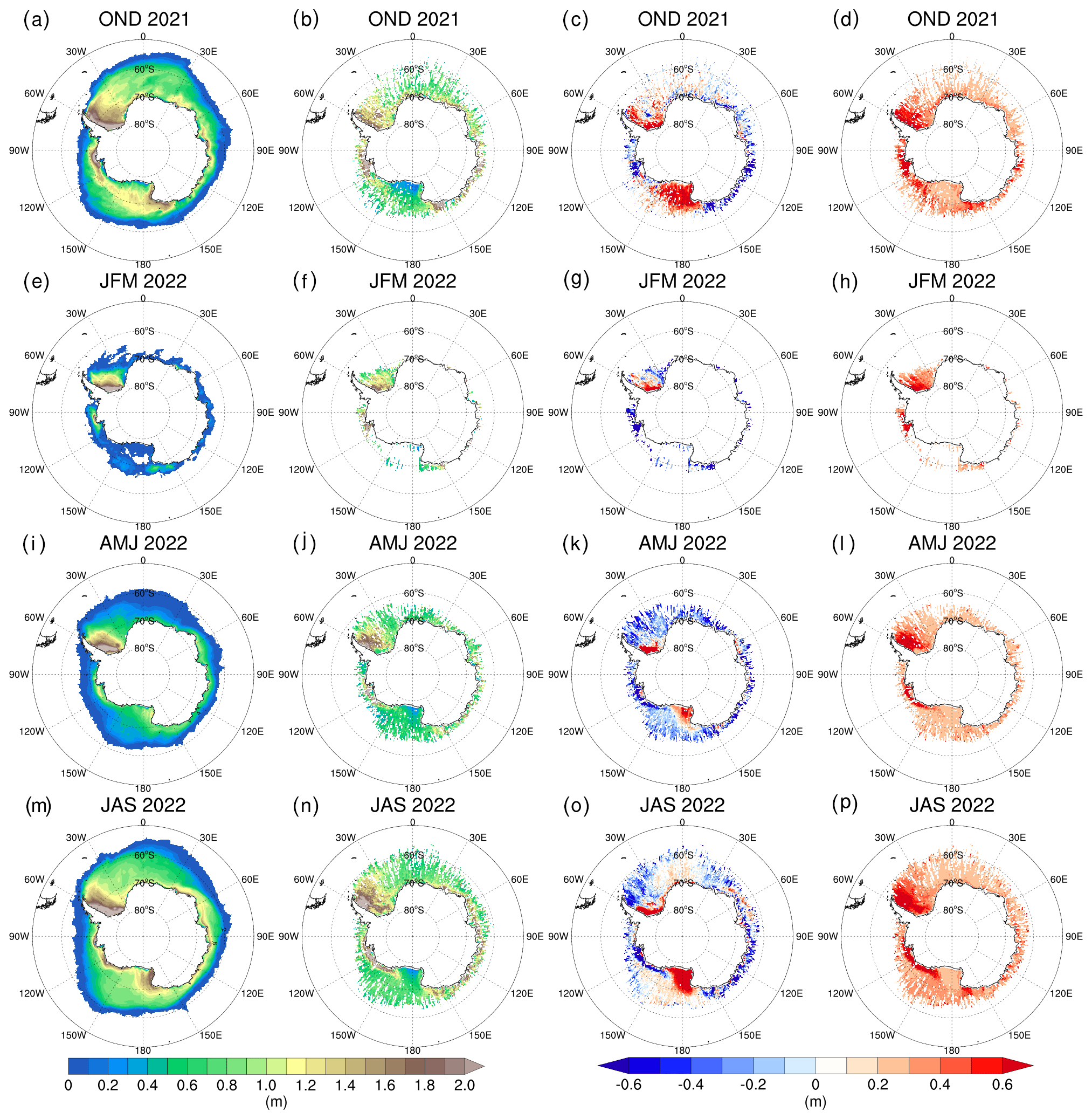
Figure 8 Seasonal patterns of the Antarctic sea ice thickness. The columns from left to right denote the DA_Forecast run at a lead time of 24 h, the ICESat-2 observations and their deviations, and the uncertainties in the ICESat-2 observations, respectively. The panels from top to bottom denote October–December, January–March, April–June, and July–September, respectively.

3.4 Sea ice drift

The Polar Pathfinder daily Antarctic sea ice motion product provided by the National Snow and Ice Data Center (NSIDC; Tschudi et al., 2019) is used to assess Antarctic sea ice drift forecasts. This data set is projected onto the EASE grid with a spatial resolution of 25 km, including input data sources derived from the Advanced Very High Resolution Radiometer (AVHRR), AMSR-E, the Scanning Multichannel Microwave Radiometer (SMMR), the Special Sensor Microwave/Imager Sounder (SSMIS), SSMIS sensors, the International Arctic Buoy Program (IABP) buoys, and the National Centers for Environmental Prediction/National Center for Atmospheric Research (NCEP/NCAR) reanalysis.

To validate sea ice drift forecasts, we convert the NSIDC ice drift components (u_o, v_o) on the EASE coordinates into the ice drift components (u_m, v_m) on the model coordinates. Sea ice drift direction, expressed by the angle α with reference to the location-dependent coordinate of u_m, is derived as the four-quadrant arctangent of (u_m, v_m). Note that α ranges between −180 and 180°. Sea ice drift direction bias is represented by the MAE of α between the modeled and observed sea ice drift. Sea ice drift magnitude is independent of selected coordinates.

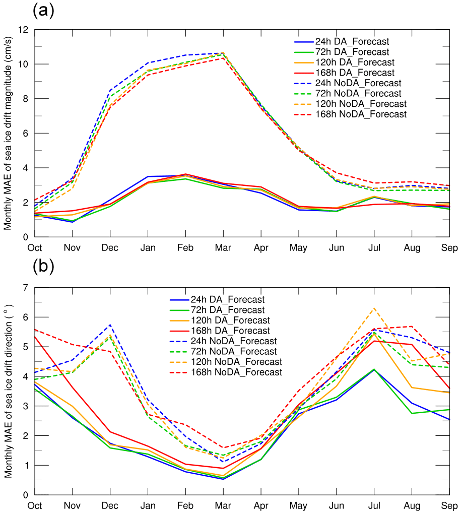
Figure 9 Time series of the monthly mean MAEs of the (a) magnitude and (b) direction of the sea ice drift forecasts at different lead times with respect to the NSIDC data. The blue, green, yellow, and red lines denote the sea ice drift forecasts at lead times of 24, 72, 120, and 168 h, respectively. The solid and dashed lines denote the DA_Forecast and NoDA_Forecast runs, respectively.

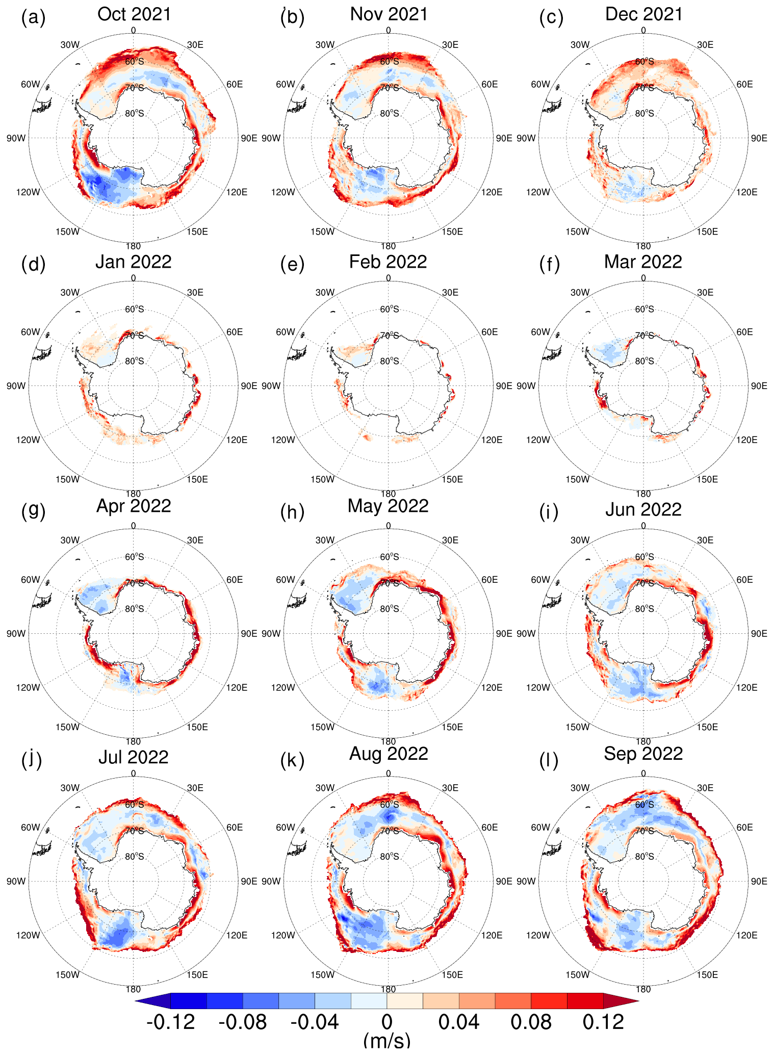
Figure 10 Monthly patterns of the magnitude bias in sea ice drift between the DA_Forecast run at a lead time of 24 h and the NSIDC data. Panels (a)–(l) denote October 2021–September 2022.

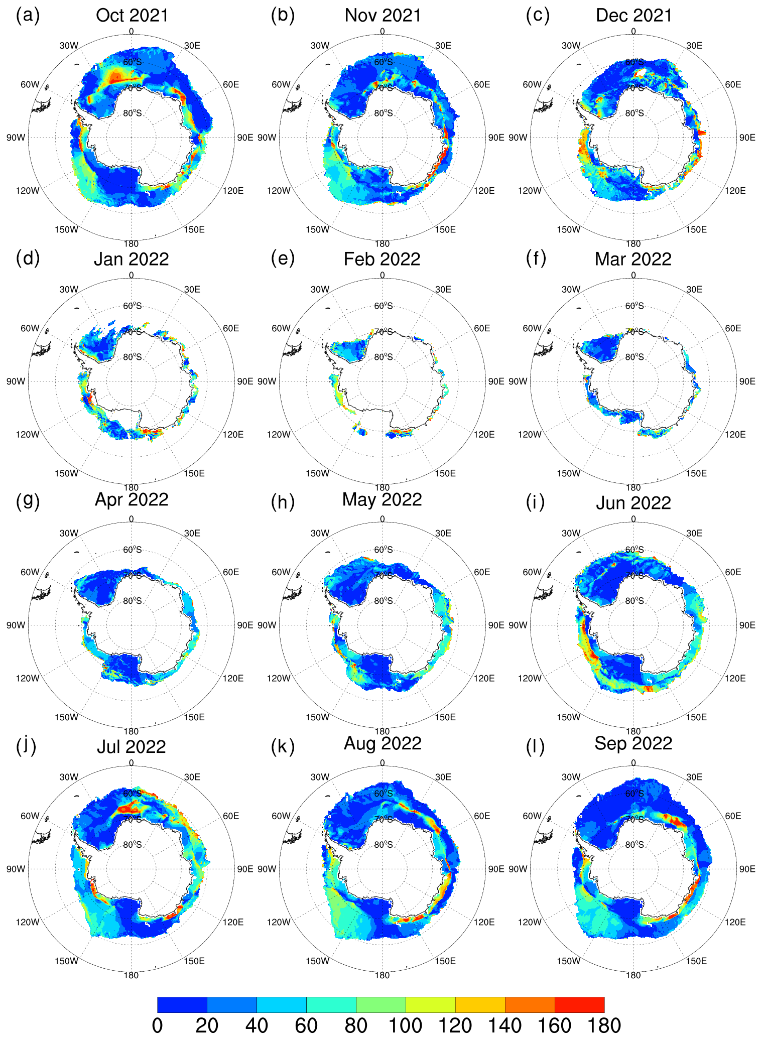
Figure 11 Monthly patterns of the direction bias in sea ice drift between the DA_Forecast run at a lead time of 24 h and the NSIDC data. Panels (a)–(l) denote October 2021–September 2022.

Validation results (Fig. 9) show that the MAEs of sea ice drift magnitude between the DA_Forecast run and observations increase during November–February and decrease during March–May. In contrast, the MAEs of sea ice drift direction between the DA_Forecast run and observations decrease during October–February and increase during March–July. Comparison between the DA_Forecast and NoDA_Forecast runs shows that the DA_Forecast run performs better than the NoDA_Forecast run, in both magnitude and direction of sea ice drift forecasts. The improvement in sea ice drift forecasts originates in principle from the enhancement of the SOIPS forecasts for sea ice concentration and thickness, induced by the data assimilation of the observed sea ice concentration, since sea ice drift is impacted by both sea ice concentration and thickness (Leppäranta, 2011).

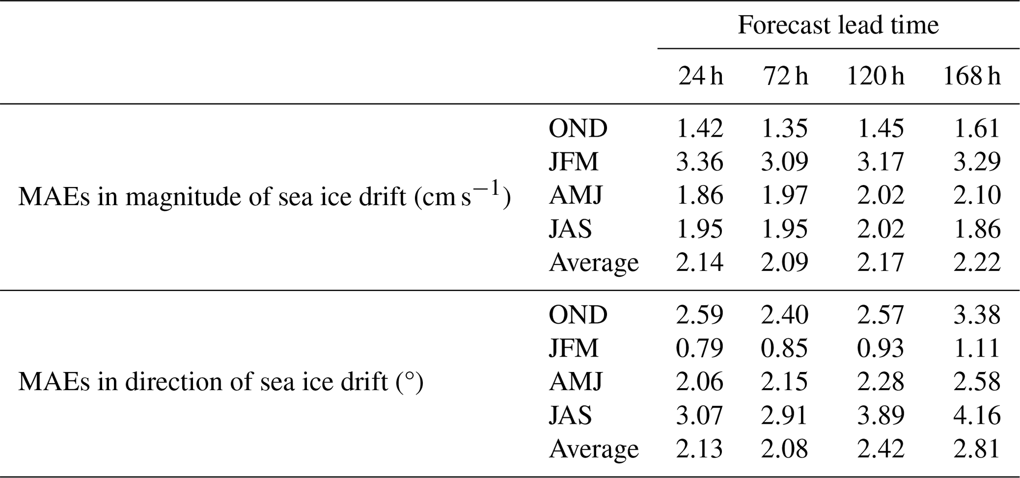
As the forecast lead time increases, the MAEs of the sea ice drift magnitude do not exhibit significant amplification, but those of direction grow significantly at a lead time of 168 h in October–November and June–September. Statistical analysis (Table 1) shows that in the DA_Forecast run, the annual mean forecasting errors in sea ice drift magnitude at lead times of 24, 72, 120, and 168 h are 2.14, 2.09, 2.17, and 2.22 cm s⁻¹, respectively. As a reference, the derived NSIDC sea ice drift magnitudes are 10.22 cm s⁻¹ during October–December, 4.78 cm s⁻¹ during January–March, 10.55 cm s⁻¹ during April–June, and 13.26 cm s⁻¹ during July–September. The annual mean forecasting errors in sea ice drift magnitude at a lead time of 168 h account for 23 % of the observed magnitude. The annual mean forecasting errors in sea ice drift direction at lead times of 24, 72, 120, and 168 h are 2.13, 2.08, 2.42, and 2.81°, respectively. These results suggest that the SOIPS has a reliable performance in forecasting sea ice drift direction, although with a systematic positive bias in the sea ice drift magnitude. A previous study conducted for the Arctic region has also found that the numerical overestimation of sea ice drift speed is a common feature in CMIP6 models (Wang et al., 2023).

Spatially, the DA_Forecast run at a lead time of 24 h produces larger sea ice drift magnitude in the north marginal sea ice zone and the coastal areas, while in between the DA_Forecast run produces smaller sea ice drift magnitude (Fig. 10). During January–March, the Antarctic sea ice zone shrinks to its annual minima, and sea ice drift magnitude bias appears to be relatively small compared to the other months. In other months, large biases in sea ice drift direction forecasts also occur in the densely packed sea ice zone, especially in the Bellingshausen–Amundsen–Ross seas and the southeastern Antarctic Ocean sector (Fig. 11); thus the MAEs in sea ice drift direction forecasts are large.

Table 1 The seasonal mean MAEs in the magnitude and direction of the DA_Forecast run at different lead times with respect to the NSIDC data.

3.5 Sea ice convergence rate

Sea ice convergence rate (SICR), defined as $\text{SICR}=-(\partial u_{\mathrm{m}}/\partial x+\partial v_{\mathrm{m}}/\partial y)$ (negative value represents sea ice dispersion; positive value represents sea ice accumulation), is a useful metric for guiding ship navigation in the sea ice zone. The Chinese Zhongshan Station in Antarctica is located at 69°22^′24.76^′′ S, 76°22^′14.28^′′ E in Prydz Bay (Fig. 12). In southern Prydz Bay, there is a large area of landfast ice. Drifting sea ice occupies the area north of the landfast ice zone. Under the forces of wind and tide, the drifting sea ice zone sometimes closely adheres to the landfast ice zone and sometimes remains separated from it, creating an open water band between them.

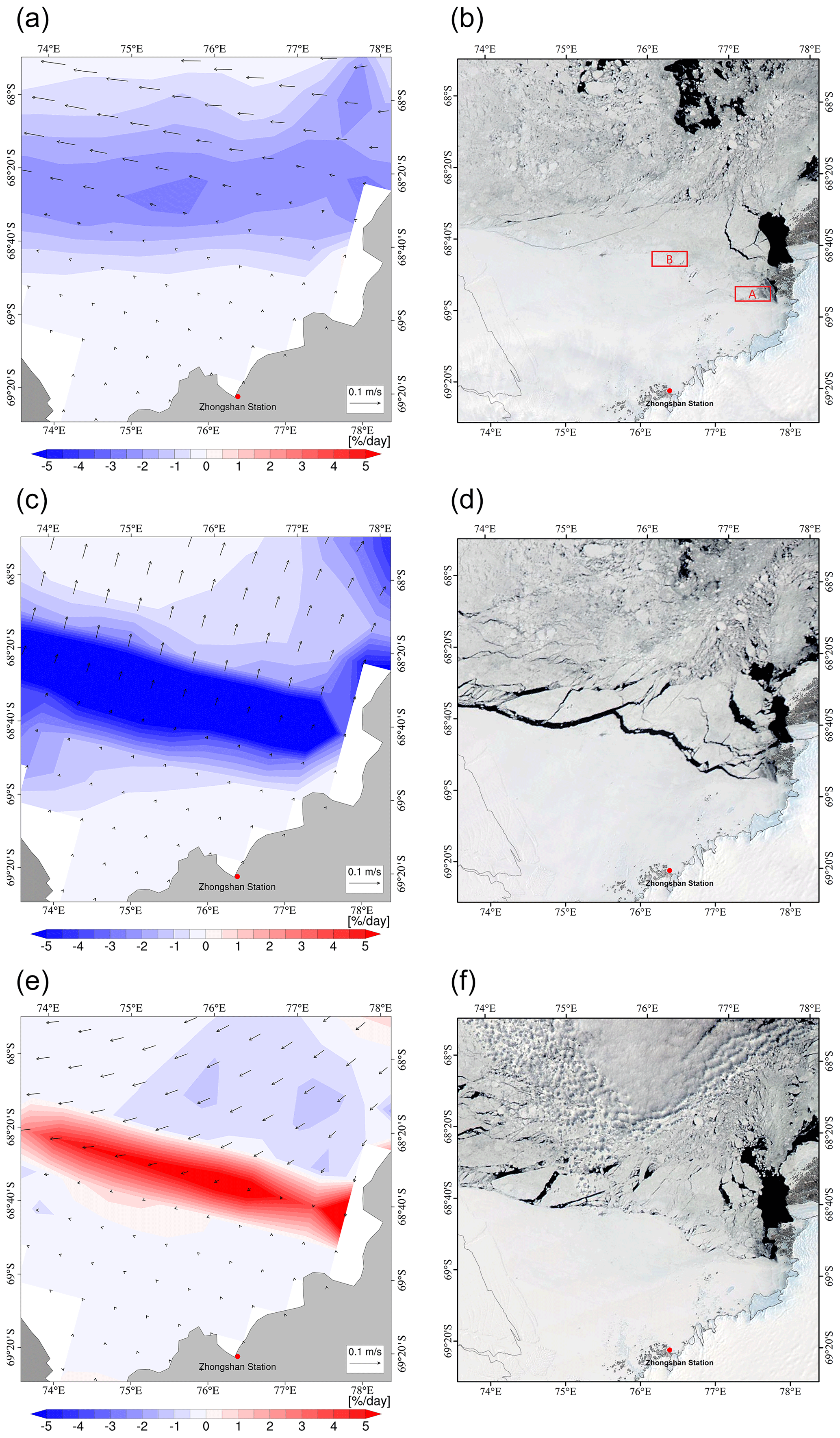
Figure 12 Sea ice convergence rate in the DA_Forecast run (a, c, e) and MODIS satellite images (b, d, f). The top, middle, and bottom panels denote forecasts/observations on 19, 20, and 21 November 2021, respectively. The forecast was initialized on 18 November 2021. The black arrows in the left column denote sea ice drift vectors, while the red and blue contours indicate that sea ice drift in the corresponding area tends to be convergent and divergent, respectively. The red dot in each panel marks the Chinese Zhongshan Station in Antarctica. The two boxes in (b) denote two areas where the icebreaker MV Xue Long has arrived in some years.

The Chinese icebreaker MV Xue Long has navigated to the Chinese Zhongshan Station in Antarctica to unload supplies almost every year for the past 4 decades. In some years, the icebreaker navigated southward to arrive at area A through the relatively loose-drifting sea ice zone in eastern Prydz Bay. However, owing to the indurative ice condition with many ice ridges and neaped icebergs in the landfast ice zone south of area A, the icebreaker had to navigate to area B and then turn southward, heading toward the Chinese Zhongshan Station in Antarctica. The landfast ice condition in the areas south of area B is more favorable to the icebreaker. As a consequence, the timing of the open water band between the drifting sea ice zone and the landfast ice zone plays a crucial role in the icebreaker's navigation from A to B.

Here we show a typical situation of how the sea ice convergence rate guides the navigation from A to B. Forecasting initialized on 18 November 2021, and the DA_forecast run at lead times of 24, 48, and 72 h suggested a weak sea ice dispersion on 19 November 2021, a strong sea ice dispersion on 20 November 2021, and a strong sea ice accumulation on 21 November 2021. The ice convergence rate forecasts indicated the open water band between the drifting sea ice zone and the landfast ice zone may occur on 19 November 2021, is very likely to occur on 20 November 2021, and may disappear on 21 November 2021. The NASA MODIS images taken on these 3 d clearly validate the usability of the sea ice convergence rate forecasts during this opening–closing process of the open water band. Further analysis shows that the forecasting skill of sea ice convergence largely originates from the precise atmosphere forcing rather than the effects of the sea ice concentration data assimilation (not shown).

4 Conclusion and discussion

In this work we introduce an operational synoptic-scale sea ice forecasting system for the Southern Ocean, i.e., the Southern Ocean Ice Prediction System (SOIPS). The system was developed to meet the increasing demands for synoptic-scale Antarctic sea ice forecasts both at present and in the coming decade. The system is configured on an Antarctic regional sea ice–ocean–ice shelf coupled model and an ensemble-based LESTKF data assimilation model and is driven by operational atmospheric forecasting variables at the ocean surface from international weather forecasting products. Near-real-time satellite sea ice concentration observations are assimilated into the system on a daily basis to update sea ice concentration and thickness in the 12 ensemble members of the model state. The SOIPS forecasts were engaged in sea ice service for the 38th Chinese National Antarctic Research Expedition for the first time.

By evaluating sea ice forecasts in a complete melt–freeze cycle between 1 October 2021 and 30 September 2022, this study finds that the SOIPS has a reliable ability to forecast sea ice evolution on a synoptic scale. With respect to the OSI SAF data, the sea ice concentration RMSEs of the SOIPS forecasts at a lead time of up to 168 h are generally lower than 0.15 during June–September, while they are close to 0.2 during January–February, and the annual mean RMSEs are lower than 0.19. Relatively large RMSEs are mainly located in the north marginal ice zone surrounding Antarctica. The AMSR2 sea ice concentration data are assimilated into the ensemble of model restart fields on a daily basis, and an analyzed (updated) ensemble of model restart fields combining the modeled and observational sea ice states is generated, which is further integrated for 168 h and driven by atmospheric forcing. The forecasts include not only the observational information, but also the sea ice changes generated by the model's physics. This causes the smaller sea ice concentration RMSEs of the SOIPS forecasts in comparison with those of the AMSR2 data, especially at lead times of 24 and 72 h in January–early March and May–September. On the other hand, large sea ice concentration RMSEs appear in most areas of the sea ice zone around Antarctica in March–April, suggesting that the model has a relatively low capacity to correctly simulate the sea ice growth rate during this onset-to-rapid-freezing period. This probably originates from the fact that the sea ice model in the SOIPS uses the zero-layer ice/snow thermodynamics, which is simple compared to sophisticated multi-layer ice/snow thermodynamics. Additionally, as a reference, the sea ice concentration RMSE of the GIOPS forecasts at a lead time of 168 h maintains below 0.35 in the year 2011 with respect to the Interactive Multisensor Snow and Ice Mapping System ice extent product (Helfrich et al., 2007). With respect to the OSI SAF data, the sea ice concentration RMSE of the SOIPS forecasts at a lead time of 24 h is larger than that of the MOI product. It should be mentioned that the MOI product assimilated the OSI SAF sea ice concentration data, which leads to a lower RMSE in comparison to the SOIPS forecasts (Fig. S4 in the Supplement).

The IIEEs of the SOIPS forecasts in most freezing months at lead times of 24 and 72 h maintain around 0.5×10⁶ km² and below 1.0×10⁶ km², respectively. In comparison with July–December, the sea ice zone is smaller during January–June, so the IIEE grows moderately in response to prolonged forecast lead times. Moreover, the sea ice edge is located further north during July–December, and the marginal ice zone is closer to the ACC-impacting areas where active oceanic and atmospheric dynamical processes promote the amplification of the IIEE along with the prolonging of forecast lead time. It should be mentioned that the mismatch in sea ice edges in some nearshore areas originates from the divergence of coastlines, ice shelf fronts, or unrealistic landfast ice zones in the model domain and the OSI SAF data.

The sea ice thickness MAEs of the SOIPS forecasts at a lead time of 24 h and the ICESat-2 observations are lower than 0.3 m, which is in the range of the ICESat-2 uncertainties. The SOIPS also performs well in forecasting sea ice drift, in both magnitude and direction. Statistical analysis suggests that annual mean forecasting errors in sea ice drift at a lead time of 168 h with respect to the NSIDC sea ice motion data are 2.22 cm s⁻¹ in magnitude and 2.81° in direction. Furthermore, the sea ice convergence rate, which can be derived from sea ice velocity forecasts, has great potential for supporting ship navigation on a fine local scale. A typical application of how sea ice convergence rate forecasts benefit the icebreaker navigation in Prydz Bay is illustrated. We realize that an improvement in sea ice convergence rate forecasts may be achieved if we introduce a landfast ice parameterization into the SOIPS, which is considered a key area for future model development. Since the included ice shelf model does not simulate collapse of ice shelf (Ochwat et al., 2024), and the ice shelf topography remains unchanged in the SOIPS, replacing the simple static ice shelf modular by a sophisticated thermodynamic–dynamic ice shelf model may further improve the performance of the SOIPS in sea ice forecasts.

Satellite observations of sea ice concentration, thickness, and drift have been used to estimate sea ice production and transport in the Antarctic coastal polynyas (Drucker et al., 2011; Nihashi et al., 2017; Tian et al., 2020). However, due to the relatively scarce coverage of satellite observations in the Antarctic, especially in sea ice thickness, the evaluation of the SOIPS sea ice forecasts in this work still has considerable uncertainties. Part of the evaluation uncertainties comes from the observational uncertainties themselves, and part comes from the differences in spatial–temporal resolutions, as well as the coastline, between the SOIPS and the observations. Accurate short-term sea ice forecasts rely on optimized initial conditions at the forecasting onset, precise atmospheric forcing data (Pascual-Ahuir and Wang, 2023) if using an ice–ocean coupled model, and model physics in representing the sea ice melt–freeze process and its heat and momentum exchanges with the underlying ocean. Specifically, the complex interactions among the atmosphere, sea ice, ocean, ice shelf, and ice sheet in the Antarctic region make the Antarctic sea ice forecasts more difficult. Moreover, in Antarctic regional sea ice–ocean modeling, how to deal with oceanic open boundary conditions is a big challenge since the broad mid-latitude ocean surrounding Antarctica can impact the Antarctic ocean and sea ice from all directions, i.e. the southern Pacific Ocean, southern Atlantic Ocean, and southern Indian Ocean. Utilizing climatological monthly mean oceanic boundary conditions from ECCO2 data results in the lack of interannual variance at the model open boundary originating from ocean variability in lower latitudes. Although the Antarctic sea ice forecasts based on global models (Blockley et al., 2014; Posey et al., 2015; Smith et al., 2016; Lellouche et al., 2018; Johnson et al., 2019) and carried out by international weather forecasting centers avoid the problem of dealing with oceanic boundary conditions, this newly developed regional sea ice forecasting system can operationally provide available sea ice forecasting information for the Southern Ocean at a moderate resolution and a high computational efficiency.

We have successfully applied synchronized assimilation of satellite-observed sea ice concentration, sea ice thickness, and sea surface temperature in our sea ice forecasting system for the Arctic, i.e. the Arctic Ice Ocean Prediction System (Mu et al., 2019; Liang et al., 2019). Owing to the rarity of operational satellite sea ice thickness observations with high spatial–temporal coverage in the Antarctic, the current version of the SOIPS only assimilates the AMSR2 sea ice concentration observations. In future, along with the elevation of satellite observation capacity, more and more sea ice and ocean variables are scheduled to be assimilated into the SOIPS to promote its ability in the Antarctic sea ice forecasts. Additionally, more precise atmospheric forcing data, more advanced model sea ice–ocean physics, and more satellite and in situ observations are urgently needed to support numerical sea ice forecasts for the Southern Ocean.