Lagrangian tracking of sea ice in Community Ice CodE (CICE; version 5)

Sea ice models are essential tools for simulating the thermodynamic and dynamic processes of sea ice and the coupling with the polar atmosphere and ocean. Popular models such as the Community Ice CodE (CICE) are usually based on non-moving, locally orthogonal Eulerian grids. However, the various in situ observations, such as those from ice-tethered buoys and drift stations, are subjected to sea ice drift and are, hence, by nature Lagrangian. Furthermore, the statistical analysis of sea ice kinematics requires the Lagrangian perspective. As a result, the offline sea ice tracking with model output is usually carried out for many scientific and validational practices. Certain limitations exist, such as the need for high-frequency model outputs, as well as unaccountable tracking errors. In order to facilitate Lagrangian diagnostics in current sea ice models, we design and implement an online Lagrangian tracking module in CICE under the coupled model system of CESM (Community Earth System Model). In this work, we introduce its design and implementation in detail, as well as the numerical experiments for the validation and the analysis of sea ice deformation. In particular, the sea ice model is forced with historical atmospheric reanalysis data, and the Lagrangian tracking results are compared with the observed buoys' tracks for the years from 1979 to 2001. Moreover, high-resolution simulations are carried out with the Lagrangian tracking to study the multi-scale sea ice deformation modeled by CICE. Through scaling analysis, we show that CICE simulates multi-fractal sea ice deformation fields in both the spatial and the temporal domain, as well as the spatial–temporal coupling characteristics. The analysis with model output on the Eulerian grid shows systematic difference with the Lagrangian-tracking-based results, highlighting the importance of the Lagrangian perspective for scaling analysis. Related topics, including the sub-daily sea ice kinematics and the potential application of the Lagrangian tracking module, are also discussed.

1 Introduction

Sea ice floes are inherently Lagrangian points that undergo thermodynamic and dynamic changes throughout their lifetime. Under the dynamic forcings from the atmosphere and the ocean, sea ice drifts, and, as internal stress accumulates, it deforms and undergoes plastic failures. The drift of sea ice floes is associated with constant thermodynamic growth and melt of the sea ice; hence it is fundamental to the energy and ice–water balance in the polar regions (Haas, 2009). Furthermore, highly nonlinear and anisotropic linear kinematic features manifest with the sea ice deformation fields, which prevail from meters to the geophysical scales (Marsan et al., 2004). The accurate observation and modeling of the sea ice drift and deformation are key to our scientific understanding of both the climate system and human activities in the polar region.

Due to the harsh conditions of the polar environment, the long-term direct measurements of the sea ice are usually carried out through in situ deployments of buoys. These autonomous systems, which are usually attached to the sea ice, relay information about their locations, sea ice conditions, and associated atmospheric and oceanic conditions. Since they drift with the sea ice, their locations are also representative of the sea ice floe to which they are attached. For example, the International Arctic Buoy Programme (IABP; https://iabp.apl.uw.edu, last access: 8 September 2024) compiles historical and real-time buoy measurements in the Arctic region. The data are widely used in the study of sea ice dynamics (Rigor et al., 2002) and thermodynamic processes (Perovich et al., 2014), as well as the data assimilation for numerical weather forecasts (Inoue et al., 2009).

The drift and the deformation of sea ice are the result of its dynamic response to the atmospheric and oceanic forcings. Unlike the Newtonian fluids of air and water, sea ice patches undergo multi-fractal deformation characterized by localized plastic faults. This highly localized and anisotropic deformation typically corresponds to sea ice leads and ridges, manifesting as linear kinematic features (LKFs; Kwok et al., 1998). While sea ice ridging is a major way that thick sea ice is formed, leads serve as important sources of heat and moisture for the polar regions, especially during winter (Rothrock, 1975; Andreas and Cash, 1999). Therefore, sea ice deformation is crucially important for the coupled climate system of the polar region. In order to study how the sea ice deforms, we usually carry out multi-scale analysis through the statistics of the deformation rates (i.e., the speed at which the sea ice deforms). Specifically, the deformation rates, denoted $\dot{\mathit{ϵ}}$'s, can be computed for individual sea ice patches at various temporal and spatial scales. Since the sea ice is constantly drifting, the computing of $\dot{\mathit{ϵ}}$'s and the related analysis should also be carried out from a Lagrangian perspective. Satellite remote-sensing-based datasets such as RGPS (Lindsay and Stern, 2003) utilize synthetic aperture radar (SAR) images collected at various times to produce large-scale, high-resolution maps of the sea ice drift and deformation. In particular, both the correlation-based and the feature tracking approaches when processing the SAR images ensure that the analysis of the drift/deformation is Lagrangian by nature. These datasets are widely used for the study of multi-scale sea ice kinematics (Marsan et al., 2004) and the validation of numerical simulations (Kwok et al., 2008; Rampal et al., 2019).

For the simulation of sea ice and its kinematics, we construct numerical models which involve a layered structure with the following: (1) the mathematical modeling of the physical processes, (2) the numerical treatments for the spatial–temporal discretization and the integration, and (3) the code implementation and the simulation on parallel computers. Popular sea ice models, such as CICE (Community Ice CodE; https://github.com/CICE-Consortium/CICE, last access: 8 September 2024) and SI³ (Vancoppenolle et al., 2023), are usually based on spatial discretization using locally orthogonal structured grids. Rheology models (Bouchat et al., 2022; Hutter and Losch, 2020) such as viscous–plastic (VP; see also elastic–viscous–plastic (Hunke and Lipscomb, 2008)) are capable of reproducing certain statistics of the observed multi-scale sea ice kinematics (Kwok et al., 2008). However, the model's output, including the instantaneous and the average model status at different temporal scales, is typically defined on the model's native Eulerian grid. One notable exception is neXtSIM, which is based on Lagrangian moving mesh and inherently supports the scaling analysis (Rampal et al., 2019). But for CICE and many widely adopted sea ice models, the model output is insufficient, especially for the scaling analysis at large temporal scales, since it inherently requires a Lagrangian perspective. A typical practice to overcome this limitation is to reconstruct Lagrangian tracks with the model's output, such as those derived from daily velocity fields in Bouchat et al. (2022). Certain limitations are still present, however, especially given the ever-growing resolution of current models (Xu et al., 2021; Zhang et al., 2023). High-frequency model output is needed to reconstruct realistic Lagrangian tracks, entailing substantial data storage and offline computation. Furthermore, the analysis of small-scale sea ice deformation (i.e., minute scale as in Oikkonen et al., 2017) requires even finer spatial and temporal model output and a larger overhead with the offline tracking analysis. Therefore, more flexible Lagrangian diagnostic tools are needed for the scaling analysis of sea ice kinematics and future development of sea ice models.

In this paper we introduce the online Lagrangian tracking of sea ice and its model integration in the model of CICE (version 5). The tracking of sea ice is carried out along with the model's numerical integration, and it supports very high frequency tracking (at the model's time step) and large numbers of Lagrangian points. The model integration is carried out and further validated through the numerical experiments in the coupled framework of Community Earth System Model (CESM, version 2: https://www.cesm.ucar.edu/models/cesm2, last access: 8 September 2024). Specifically, the comparison with observed buoy tracks is carried out with atmospherically forced historical simulations. Furthermore, a high-resolution experiment with 7 km resolution in the Arctic region is carried out, and we evaluate the spatial–temporal scaling of wintertime sea ice deformation. In Sect. 2 we introduce the tracking algorithm and the integration in CICE in detail. Section 3 includes the numerical experiments and detailed analysis of simulation results. Finally in Sect. 4, we summarize the article and discuss related topics, including potential applications of the sea ice Lagrangian tracking and the high-resolution simulation of sea ice kinematics.

2 Lagrangian tracking in CICE

The Lagrangian tracking of sea ice is tightly integrated with the dynamics processes of CICE (version 5). The model grid of CICE is a two-dimensional, logically rectangular, structured grid with the size of (nx_global,ny_global) and indexed by (i,j). Typical lateral boundary conditions are supported for global configurations, including the east–west periodic boundary and the tripolar grid boundary (Murray, 1996). For the Lagrangian tracking, each active point has a specific logical location of (x,y) in the two-dimensional continuous space, satisfying $\mathrm{0}\le x<$nx_global and $\mathrm{0}\le y<$ny_global. Furthermore, there is a bi-projection between each point’s logical location and its corresponding geolocation. The Lagrangian tracking is carried out within the model grid's domain following the tracking algorithm while maintaining the grid's lateral boundary conditions and the land–ocean distribution.

In this section, the Lagrangian tracking algorithm is introduced in detail in Sect. 2.1, which is based on the existing advection framework of transport remapping (Dukowicz and Baumgardner, 2000). Regarding the commonly used functionality of CICE, the Lagrangian tracking also supports parallel computing, tripolar grids and a simple logging system for the record of the tracking results. Detailed implementation and the integration in CICE are covered in Sect. 2.2.

2.1 Lagrangian tracking algorithm

The Lagrangian tracking algorithm is based on the transport remapping advection scheme, which is available in CICE (Dukowicz and Baumgardner, 2000). As a conservative, two-dimensional, semi-Lagrangian scheme, transport remapping operates on the Arakawa-B staggered grid. At each dynamics step of CICE, the backward tracking of the corner points is carried out for the advection of tracers onto the Eulerian grid cells (corners of the hollow quadrilateral in Fig. 1a). For the Lagrangian tracking, we utilize the backward tracking vectors and compute the forward tracking for all four corner points (filled grey arrows in Fig. 1a), and they form the new quadrilateral (outlined in blue). Then, based on the previous location of the Lagrangian point (black circle), we can compute its new location (blue circle) as follows.

The tracking of the Lagrangian point is based on the local, normalized coordinate of the grid cell containing the point. Under the local coordinate, the cell's four corners correspond to (0.0,0.0), (0.0,1.0), (1.0,0.0) and (1.0,1.0), respectively. The previous location of the Lagrangian point under this coordinate is (x_local,y_local), satisfying $\mathrm{0}\le x_{\mathrm{local}}<\mathrm{1}$ and $\mathrm{0}\le y_{\mathrm{local}}<\mathrm{1}$. Note that given the point's logical position in the model grid as (x,y), the following points hold: (1) the cell where the point is present has the index of $(\lfloor x\rfloor +\mathrm{1},\lfloor y\rfloor +\mathrm{1})$, and (2) $x_{\mathrm{local}}=x-\lfloor x\rfloor$ and $y_{\mathrm{local}}=y-\lfloor y\rfloor$. After the forward tracking, the four corners have the new locations of $(x_{i,j},y_{i,j})$ for $i\in \mathit{\{}\mathrm{0},\mathrm{1}\mathit{\}}$ and $j\in \mathit{\{}\mathrm{0},\mathrm{1}\mathit{\}}$. Then, the new location of the Lagrangian point, denoted $(x_{\mathrm{local}}^{*},y_{\mathrm{local}}^{*})$, is computed through the bilinear interpolations with x_i,j's and y_i,j's, assuming that its relative location within the new quadrilateral remains (x_local,y_local). In the case that $x_{\mathrm{local}}^{*}$ or $y_{\mathrm{local}}^{*}$ is larger than 1 or smaller than 0, the Lagrangian point has drifted out of the current grid cell, which we denote as the migration of the point. Since CICE utilizes domain decomposition for parallel computing, the migration potentially is between blocks (sub-domains after decomposition) and entails communication between parallel processes. The detailed support is introduced further in Sect. 2.2.

Based on the geolocations of the four cell corners and the Lagrangian point's relative location within the cell, we can compute the geolocation of the Lagrangian point. Specifically, first, the three-dimensional locations of the cell corners are computed with their latitudes and longitudes. Through linear interpolations, we locate the three-dimensional location of the Lagrangian point. Finally, the latitude and longitude of the Lagrangian point can then be determined.

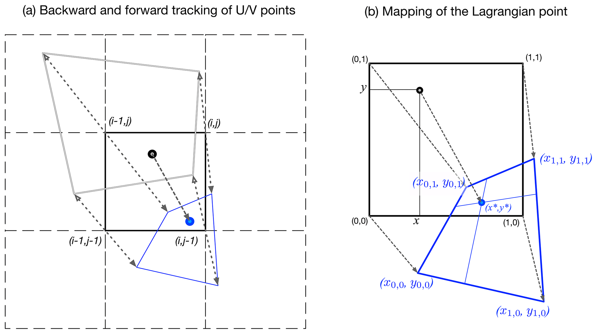
Figure 1 Local Lagrangian tracking scheme. Panel (a) shows the backward tracking (the double-lined quadrilateral) and the forward tracking (the quadrilateral in blue) of the corners of the current T cell at (i,j) (thick black quadrilateral). In panel (b), the tracking of a Lagrangian point (black circle) at a normalized relative position (x,y) within the current T cell is based on linear interpolation of the four corner points (i.e., (x_i,y_j) for $i=\mathit{\{}\mathrm{0},\mathrm{1}\mathit{\}}$ and $j=\mathit{\{}\mathrm{0},\mathrm{1}\mathit{\}}$).

2.2 Implementation in CICE

2.2.1 Software implementation

For the Lagrangian tracking in CICE, we define the data structure as lagr_point in the Fortran module of ice_transport_driver. It contains necessary fields of information for the Lagrangian point, including its current status, lifetime, current location and other essential information. Furthermore, each of the parallel CICE processes maintains a large, pre-allocated pool of available Lagrangian points (i.e., instances of lagr_point). When a new Lagrangian point is created in the current process or migrated from another process, an unused slot is claimed from this pool. Similarly, when the point is dead (i.e., due to melting) or migrates out of the block, the slot is reclaimed and recycled in the pool.

The life cycle of a Lagrangian point consists of several stages (Fig. 2) and transitions between the stages, called events. Upon its creation (type-I event), the Lagrangian point is assigned to a specific geolocation and, consequently, a specific block and a specific processor. The Lagrangian point drifts (type-II event), until the sea ice melts (sea ice concentration lower than 5 %, type-V event), or it is automatically deactivated (e.g., exceeding the prescribed maximum lifetime). When the Lagrangian points migrate outside the current block, they will be delivered to the corresponding adjacent block (type-III event; see also below). This process is carried out through the built-in boundary exchange operations of CICE. A special landing event of Lagrangian points (type-IV) is supported but not possible in the current implementation.

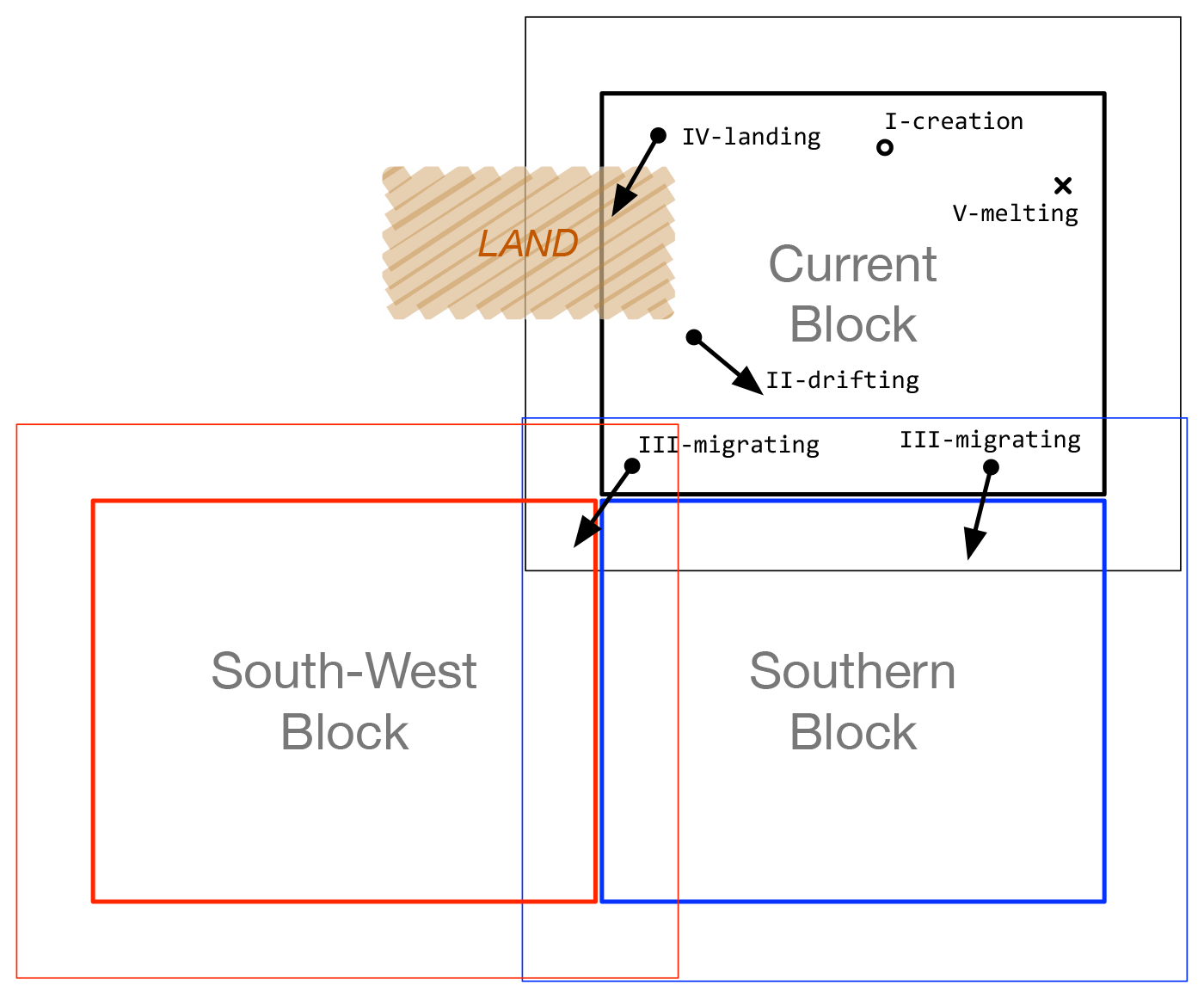
Figure 2 Typical events for Lagrangian points, including the creation, the melt (i.e., ice concentration below 5 %), drifting within a block or between blocks (i.e., migration), and migration onto lands.

2.2.2 Overall model integration

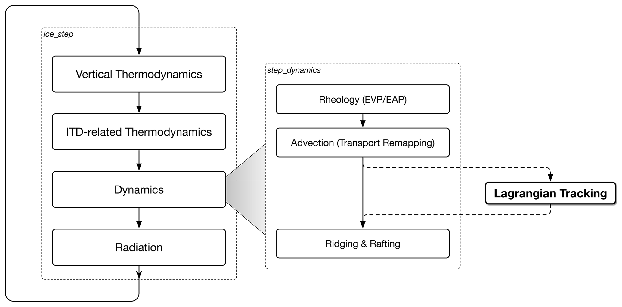
As shown in Fig. 3, the tracking of all Lagrangian points occurs within each dynamics time step (i.e., step_dynamics) after the computation of the prognostic velocities and the advection process (which computes the backward tracking vectors). To ensure numerically stable integration for the advection, there is strict limitation over the time step and hence the backward/forward tracking vectors. As a consequence, Lagrangian points cannot migrate beyond one grid cell in either direction. When a specific point migrates beyond the current block's boundary (i.e., thick rectangular boundary in Fig. 2), it will be strictly within the outer boundary of the block (i.e., within the thin rectangular boundary in Fig. 2).

The Lagrangian tracking contains four major steps (shown below). For each Lagrangian point, its status is maintained, it is tracked with the forward drifting vectors and its location information is updated. In the case of the Lagrangian point migrating outside the current block, it is recorded for further boundary exchange. Then the Lagrangian points are exchanged between blocks, with newly migrated Lagrangian points recorded for the current block.

1. For each active Lagrangian point, the following steps should be followed:

   1. Check for deactivation (due to melt, lifespan, etc.), with necessary management of the Lagrangian point slots.

   2. Increase the ge of the Lagrangian point.

   3. Retrieve the local advection information.

   4. Do Lagrangian tracking, and update the logical and the geophysical positions.

   5. Check for potential migration out of the current block.

2. For a migrating point, the following steps should be followed:

   1. Record its information for boundary exchange.

   2. Carry out management of the Lagrangian point slot.

   3. Carry out boundary exchanges for Lagrangian points.

   4. Activate newly migrated Lagrangian points.

   5. Deactivate Lagrangian points (due to landing, etc.) with necessary management steps.

Figure 3 Overall integration of Lagrangian tracking in the time step of CICE.

2.2.3 Miscellaneous

Boundary exchanges for migrating Lagrangian points

Each dynamics time step involves a single Fortran function call to the boundary exchange, carrying out the migration of Lagrangian points between blocks. The maximum exchangeable Lagrangian point count per boundary cell can be changed in the code through the Fortran parameter LAGR_BNDY_SIZE_PARAM. It is worth noting that the single boundary exchange due to the migration of Lagrangian points only incurs a very small computational overhead. Within the same dynamics time step, the elastic–viscous–plastic (EVP) solver usually contains over 100 sub-cycles of the elastic waves and the corresponding boundary exchanges (Lemieux et al., 2010; Xu et al., 2021). Furthermore, the Lagrangian tracking utilizes the transport remapping scheme's backward tracking. In general, the EVP solver dominates the overall simulation time of the sea ice dynamics, with the Lagrangian tracking consuming less than 3 % of the time for all the numerical experiments in Sect. 3.

Support for tripolar grids

Tripolar grids are commonly used in high-resolution global configurations of CICE and CESM (Small et al., 2014). For example, the 0.1° grid of TX0.1 is used for the global ocean mesoscale-resolving simulations of CESM. The commonly used U-fold tripolar grids are supported for our implementation of the Lagrangian tracking in CICE, with the schematics shown in Fig. 4.

When the Lagrangian point drifts beyond the northern boundary of the blocks on the tripolar folding line, it is passed to the corresponding block and grid cell through the boundary exchange process. This corresponds to the case with y larger than ny_global, where ny_global is the grid cell count in the j direction. Then, the x and y positions of the point are modified accordingly to the correct values, following the topology on the tripolar boundary.

Logging system

A simple text-based logging system is implemented to report the results of the Lagrangian tracking. Each parallel processor generates a log file that contains the records of all active Lagrangian points on the processor. The records include the major events, including the creation of the Lagrangian points, the melt events and the migration events, as well as the Lagrangian points' status at regular time intervals. The time step count for reporting Lagrangian points' information is a user-prescribed compile-time parameter (see Appendix C for details).

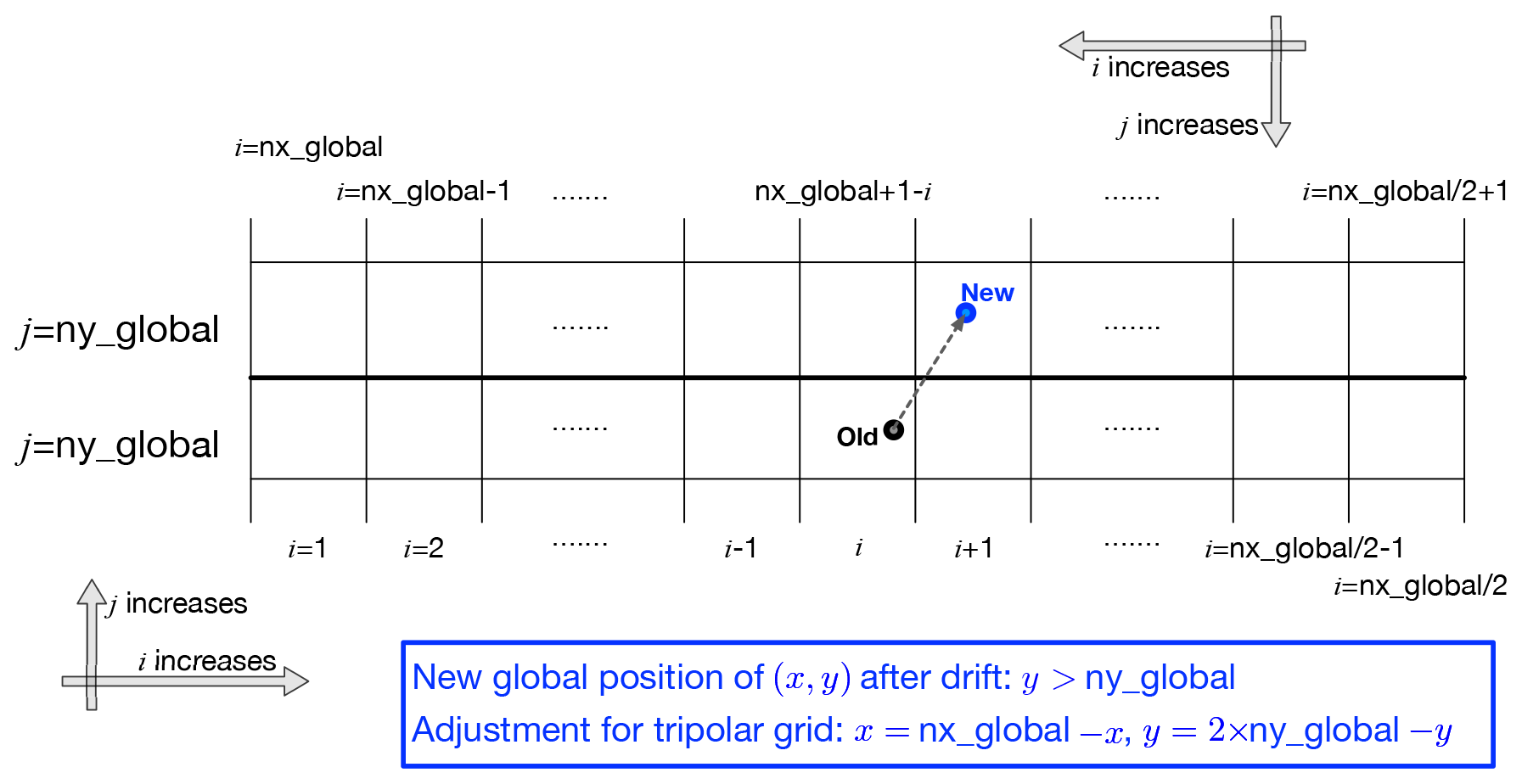
Figure 4 Support of Lagrangian point migration for tripolar grids. The model's global grid is of size nx_global by ny_global, with the northern tripolar boundary shown. U-fold tripolar grids are supported (i.e., sea ice velocities are defined on the corner points of the Arakawa-B grid and along the northern boundary).

3 Numerical experiments and analysis

We carry out numerical experiments of the Lagrangian tracking with CICE (version 5) and CESM (version 2). CICE is configured with five ice thickness categories with multiple vertical layers, as well as full thermodynamic and dynamic processes. Key model configurations include the mushy-layer vertical thermodynamics, the elastic–viscous–plastic (EVP) rheology model and the delta-Eddington radiation scheme. Detailed parameterization schemes and major parameters of CICE are further covered in Appendix A. Two model resolutions of CICE are used: the nominal 1° grid of GX1V6, which is built in in CESM, and the nominal 0.15° grid of TS015 (previously implemented in CESM (Xu et al., 2021)). Notably, the TS015 grid has a horizontal dimension of 2400×1680 globally, and the mean grid resolution is about 7 km in the Arctic region. Prominent, multi-fractal sea ice deformation can be simulated at this resolution (Xu et al., 2021).

For all the experiments, CICE is coupled to the slab ocean model (SOM) and forced by the CORE-II dataset through the coupling framework in CESM. The CORE-II dataset is based on NCEP atmospheric reanalysis and further used in the Ocean Model Intercomparison Projects (Griffies et al., 2016). It contains two separate forcing datasets: the normal year forcing (NYF), which is annually repeating, and the inter-annual forcing (IAF), which is for the years between 1948 and 2007. While the NYF dataset is usually used for the long-term simulations and the spin-up of the ocean–sea ice coupled model, the IAF dataset can be used for the hindcast of the historical states of the ocean and the sea ice (Wang et al., 2016). Both the NYF and the IAF datasets are used for the numerical experiments, covered in the rest of this section.

The simulated Arctic sea ice climatology under NYF is shown in Fig. 5. The seasonality of the sea ice extent at both 1 and 0.15° (not shown) is consistent with the observational climatology (NSIDC). The overestimation of sea ice extent (SIE) during winter months mainly manifests in the peripheral seas of lower latitudes. In particular, in the Atlantic Arctic region, the overestimation of SIE may be due to the absence of ocean heat transport of the SOM. During summer, SIE agrees well with the observation. In terms of the sea ice volume, there is general underestimation compared with PIOMAS (Schweiger et al., 2011). Thick, multi-year sea ice manifests north to Greenland and the Canadian Arctic Archipelago (CAA), with the clockwise circulation in the Canadian Basin as controlled by the Beaufort High. With the generally good agreement of the modeled sea ice states with the observational datasets, we consider it sufficient for further analysis of the Lagrangian tracking. Moreover, further improvements of the model's simulation results are planned for future work, including the coupling with a dynamic ocean model and the tuning of parameterization schemes in CICE.

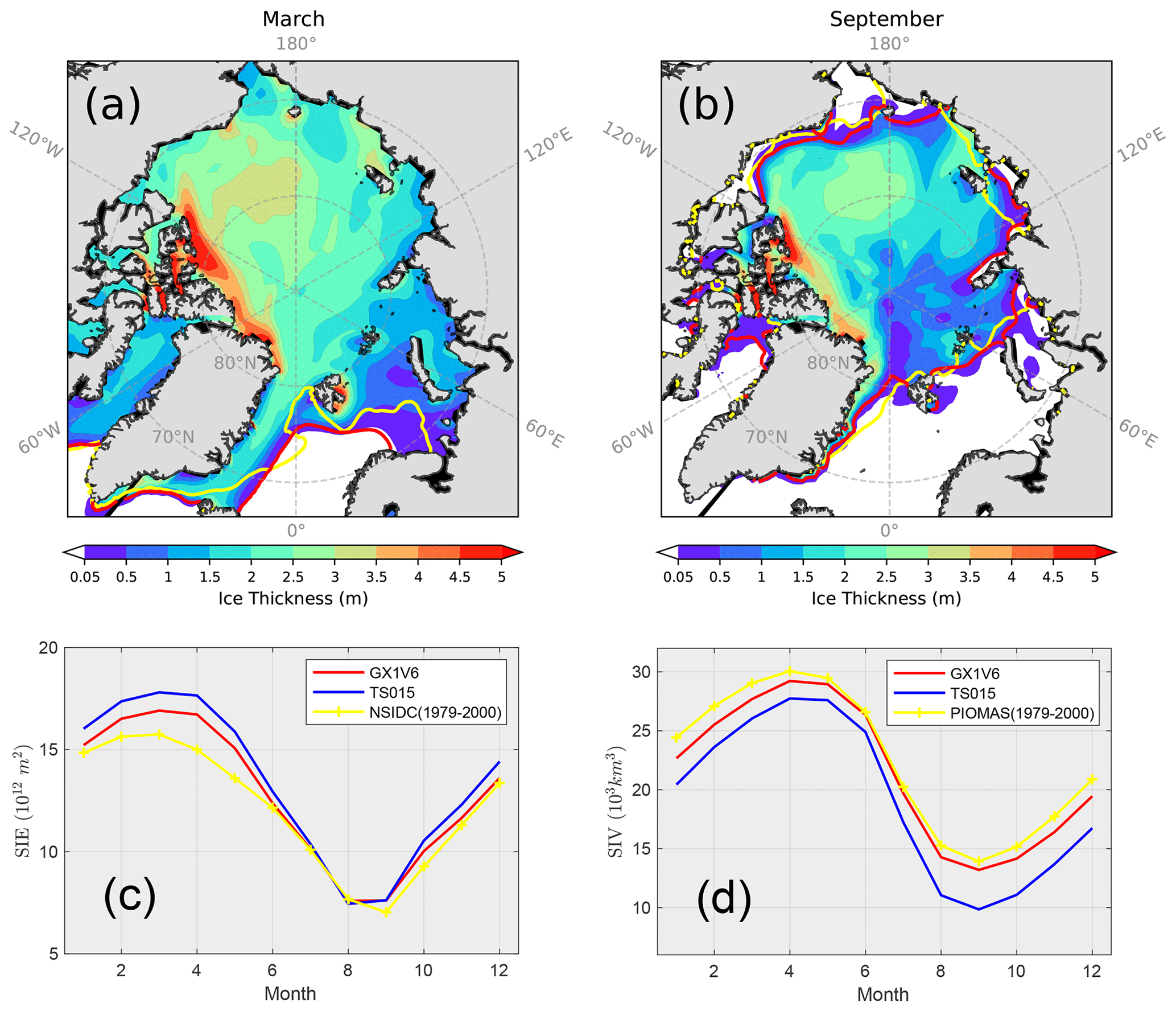
Figure 5 March (a) and September (b) sea ice thickness simulated by CESM and the GX1V6 grid. The last 10 years' results are used to compute the thickness fields (filled contour) and the ice edge with sea ice concentration (SIC) at 15 % (red line). The climatological sea ice concentration from NSIDC (based on passive microwave sensors) of the corresponding months is computed for the years between 1979 and 2000, with the sea ice edge shown by the yellow line (SIC = 15 %). The seasonal cycles of Arctic sea ice extent (SIE) and sea ice volume (SIV) are shown in panel (c) and (d), respectively. The simulation results from both GX1V6 and TS015 are included. For comparison, SIE is based on the NSIDC dataset, and SIV is computed from the PIOMAS dataset for the same period (i.e., 1979 to 2000).

3.1 Climatology of Lagrangian points under NYF

Under the annually repeating NYF dataset, we carry out the basic test of the Lagrangian tracking with the low-resolution, 1° grid. After the model has reached quasi-equilibrium after a spin-up of 20 years, we deploy one Lagrangian point at the center of every grid cell with sea ice (sea ice concentration (SIC) >5 %) in the Northern Hemisphere. The initial locations of the points are shown in Fig. 6a. With the summer melt and the transport to lower latitudes, the count of active Lagrangian points decreases with each year. After a full year since the deployment, the Lagrangian points outside the Arctic Basin are all lost due to melting (Fig. 6b). In Fig. 7 we show the 2-month tracks of the points for the first whole winter after deployment. The overall distribution of remaining points after a melt season, as well as their tracks in the winter, shows (1) the counterclockwise drift in the Beaufort Gyre at distinctive stages throughout the winter, (2) the convergence of points to the north of Greenland/the CAA, and (3) the transpolar drift from the eastern part of the basin and the outflow in the Fram Strait. After 5 years and 10 years (Fig. 6c and d), the Lagrangian points are generally lost. The surviving points are mainly retained due to the accumulation in the Beaufort Gyre. Among all of the 3599 points that are originally in the basin (80° N and further north), about 2063 (57.3 %) points are lost through melting in the basin within the first 20 years, while 1083 (30.1 %) are lost due to export from the Fram Strait (FS). In later years, the surviving points are mainly lost due to the circulation to the transpolar drift (hence the FS export) or to the eastern part of the basin with a more prominent summer melt. The daily locations of the Lagrangian points are shown by the animation in the Supplement. It is worth noting that the NYF forcing dataset does not support direct comparison with observations. Hence the experiment results, including the simulated circulation of the Lagrangian points and the loss due to melt process, provide us with a basic test of the Lagrangian tracking functionalities.

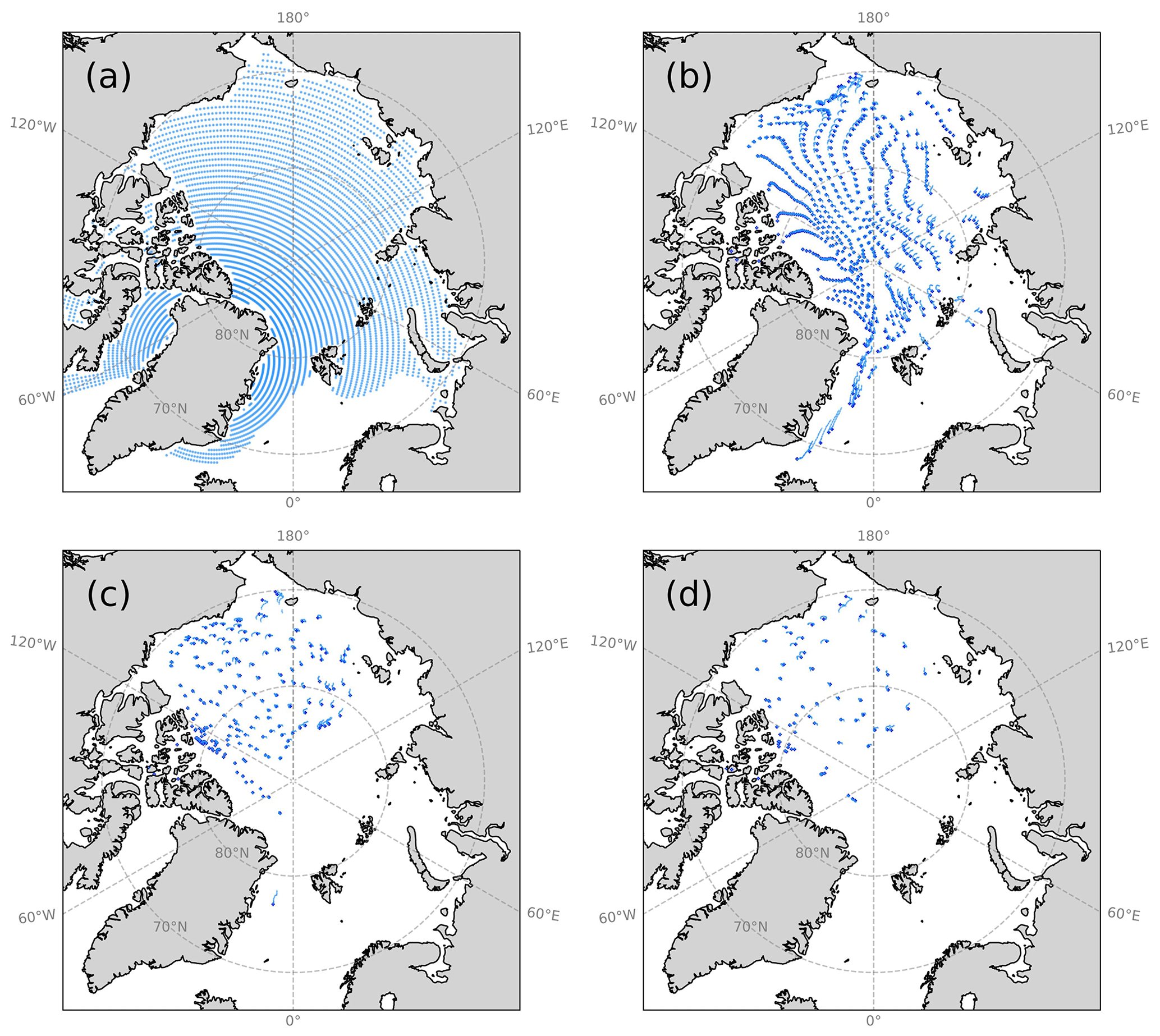
Figure 6 Lagrangian points (dots) in the initial deployment on 1 January (a), after 1 year (b), after 5 years (c) and after 10 years (d). The previous locations of each point are also shown for up to 2 weeks (lines). One in every two Lagrangian points is shown in (b), (c) and (d).

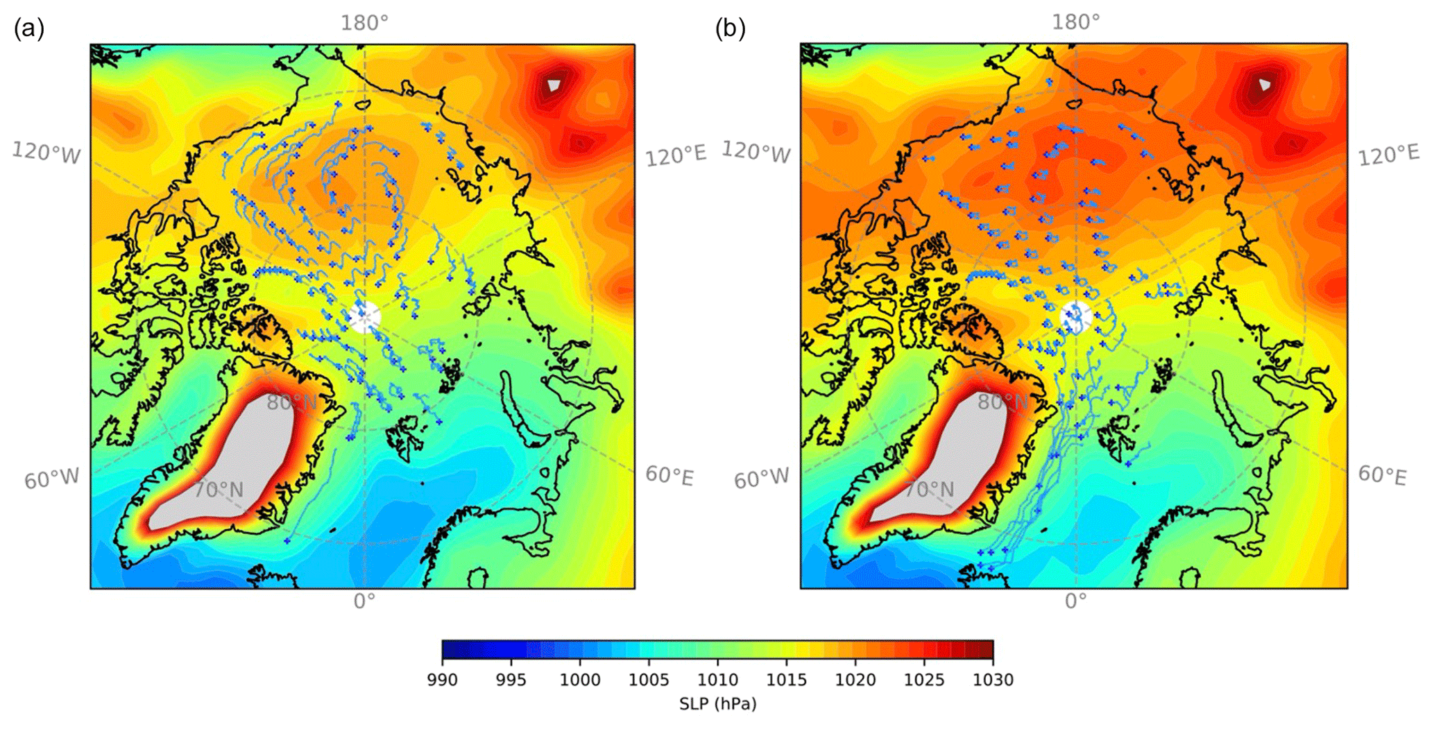
Figure 7 Sea-level pressure (SLP; filled contour) and the tracks of Lagrangian points for two bimonthly periods: November–December (a) and February–March (b) for the NYF-based simulation with the GX1V6 grid. The tracking results during the first whole winter after the deployment of the Lagrangian points are shown. One in every five Lagrangian points is indicated by the dark-blue dot, and its track throughout the two periods is indicated by the thin blue lines.

3.2 Validation of Lagrangian tracking under IAF

We further evaluate the Lagrangian tracking through the IAF-based simulation and compare it with the buoy measurements. Based on the 1° grid (GX1V6) and the model's spin-up status under NYF, we carry out the historical simulation for the years between 1979 and 2001. For every day during the winter (December to March) at 00:00 (UTC), we deploy a Lagrangian point in every grid cell where sea ice is present. For each Lagrangian point, we track its location for up to 90 d. The daily instantaneous locations of the points are recorded and further compared with the observations.

The observational dataset from the International Arctic Buoy Programme (IABP; Rigor et al., 2008) during the same years is used for validation (data available at https://iabp.apl.uw.edu/data.html, last access: 10 May 2023). Since we deploy Lagrangian points to the center of the grid cells, we use the following criteria to match the physical buoys' locations of IABP. In total, 621 buoys with 49 004 hourly locations are available for comparison. We further split each buoy's continuous track into sub-tracks of 14 d for further comparisons. For each buoy's (sub-)track, we screen over the newly deployed Lagrangian points on its starting date. The Lagrangian point nearest to the track's starting location is located, and the simulated track is then compared against the observation. Leap years are ignored in the IAF dataset and the simulations; hence the buoys' tracks starting on 29 February are matched with the Lagrangian points on 1 March.

Figure 8 shows the matching between the buoys' and the corresponding Lagrangian points' locations during the winter of 1993–1994 (December to March). All of the sub-tracks, each covering 14 d of tracking of the buoy, are shown. The two major sea ice drift regimes include the clockwise circulation in the Canadian Basin and the clockwise drift and export of the sea ice in the region east to 60° W and west to 130° E. In both regimes, the modeled Lagrangian points' tracks are highly consistent with the observations.

Furthermore, Fig. 9 shows the distance between the locations of the buoys and the corresponding Lagrangian points for all the sub-tracks. In total, there are 2849 sub-tracks for comparison, each corresponding to a buoy's drift within 14 d. For the starting locations of the buoys' sub-tracks, the average distances to the matching virtual buoys are all within 50 km. The average grid size within the Arctic Basin is about 50 km, with finer (coarser) resolution in the area near (far from) Greenland. For over 75 % of the matching buoy pairs, the initial distance is less than 27 km. After the tracking for 14 d, the distance gradually grows, but for 75 % of all pairs, the distance is within 60 km. Besides, the median (mean) distance is 38 km (43 km). On average, the drift distance of buoys is 87 km at 14 d scale. For fast-moving buoys such as those entering the Fram Strait, the distances between the Lagrangian points and the matching physical buoys are larger, but the relative error always remains low within the 2-week tracking period. In general, based on the Lagrangian tracking in CICE, the sea ice drift as simulated by the model matches buoys' observations well. The tracking uncertainties may arise from the limited spatial resolution of the model, the uncertainty of the atmospheric forcing dataset and the sea ice model's dynamics in simulating the observed drifts. Besides, due to the regular deployment of the Lagrangian points, there is no exact match of the buoys' initial locations. Further attribution of the tracking error to the various contributing factors, including the model and the data's uncertainty, as well as the initial location errors, is planned for future study.

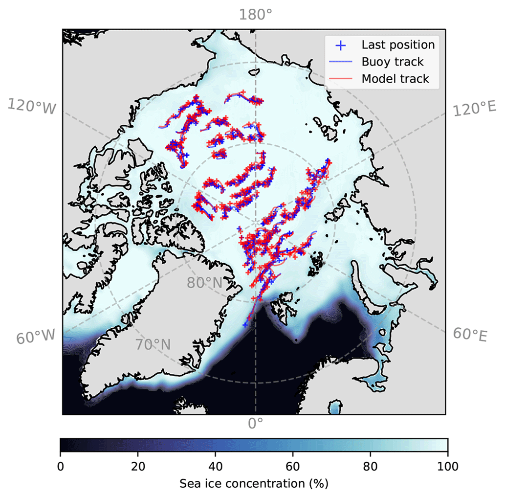
Figure 8 Simulated Lagrangian points (blue) and those of the corresponding IABP buoys (red) during the winter of 1993–1994. The last location (+) of each record and the track (line) of up to 14 d are shown for each buoy/Lagrangian point. The wintertime mean (DJFM) sea ice concentration is also shown in the background.

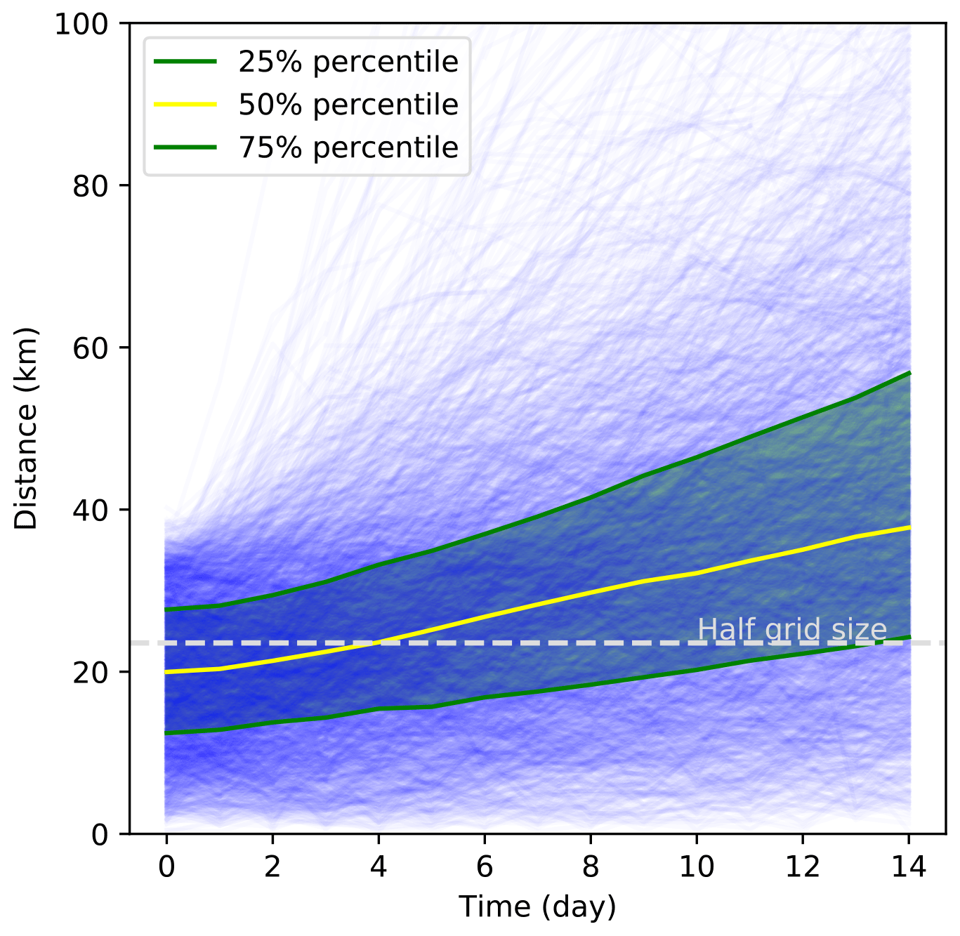
Figure 9 Distance between the modeled Lagrangian points and the corresponding buoys. The yellow line is the median, and the lower and upper edges of the green shading are the 25th and the 75th percentiles, respectively. The horizontal bar (dashed grey line) marks half of the mean grid size ($\sqrt{\mathrm{d}x\cdot \mathrm{d}y}/\mathrm{2}$) of the GX1V6 grid in the Arctic Basin.

3.3 Scaling analysis of sea ice kinematics in the 7 km resolution simulation

We further carry out high-resolution simulations of sea ice kinematics and related analysis of the sea ice deformation. In particular, with the 7 km resolution of the TS015 grid in the Arctic region, the model is capable of simulating the multi-fractal sea ice deformation (Xu et al., 2021). The experiment is based on the NYF dataset and the model's quasi-equilibrium status after the spin-up process. The Lagrangian tracking is utilized for the diagnostics of the wintertime sea ice deformation and related statistics over multiple spatial and temporal scales. We first introduce the basic framework of scaling analysis and the use of Lagrangian tracking in Sect. 3.3.1. Furthermore, the detailed analysis of the spatial scaling (Sect. 3.3.2) and the temporal scaling and the spatial–temporal coupling (Sect. 3.3.3) are covered.

3.3.1 Lagrangian tracking and scaling analysis

The sea ice deformation rates ($\dot{\mathit{ϵ}}$'s) are defined with simulated velocities. Since CICE is based on the locally orthogonal grid and Arakawa-B staggering, the model's velocity as well as the derived velocity of Lagrangian points are defined as fields of u's and v's. The grid-invariant deformation rates, including the divergence rate (${\dot{\mathit{ϵ}}}_{\mathrm{div}}$) and the shear rate (${\dot{\mathit{ϵ}}}_{\mathrm{shear}}$), are then defined as follows. The total deformation rate (${\dot{\mathit{ϵ}}}_{\mathrm{total}}$), which is subjected to further scaling analysis, can be further defined with ${\dot{\mathit{ϵ}}}_{\mathrm{div}}$ and ${\dot{\mathit{ϵ}}}_{\mathrm{shear}}$.

$$\begin{array}{}\text{(1)}& {\displaystyle }{\dot{\mathit{ϵ}}}_{\mathrm{div}}=u_x+v_y\text{(2)}& {\displaystyle }{\dot{\mathit{ϵ}}}_{\mathrm{shear}}=\sqrt{(u_x-v_y{)}^{\mathrm{2}}+(u_y+v_x{)}^{\mathrm{2}}}\text{(3)}& {\displaystyle }{\dot{\mathit{ϵ}}}_{\mathrm{total}}=\sqrt{{\dot{\mathit{ϵ}}}_{\mathrm{div}}^{\mathrm{2}}+{\dot{\mathit{ϵ}}}_{\mathrm{shear}}^{\mathrm{2}}}\end{array}$$

In these equations, u_x, u_y, v_x and v_y are the spatial derivatives of u and v in the two orthogonal directions. The direct model output of the instantaneous and/or the temporal mean of the velocity fields, as well as the various deformation rates, is defined on the Eulerian model grid. In Fig. 10 we show the maps of the daily-mean ${\dot{\mathit{ϵ}}}_{\mathrm{total}}$ in the Arctic region for 2 typical days of the experiment with TS015. LKFs manifest with the highly localized, anisotropic sea ice deformation. It is worth noting that the daily-mean velocity and the deformation fields (shown in Fig. 10) are inherently Eulerian and hence not appropriate for the scaling analysis. For example, the offline tracking (at hourly scale) should be carried out for further analysis (e.g., Bouchat et al., 2022).

The velocity derivatives at various temporal–spatial scales (i.e., $\mathit{\{}u,v{\mathit{\}}}_{\mathit{\{}x,y\mathit{\}}}$'s) are further computed over the various Lagrangian patches. A set of adjacent Lagrangian points form an enclosed sea ice patch and start with the position on regular Eulerian grid points. Their locations change with the Lagrangian tracking, due to the sea ice drift and deformation. At a certain time (delayed by T), their new locations are recorded and the displacement from their original locations are computed as Δ_x's and Δ_y's. Then the average velocity $\stackrel{\mathrm{‾}}{u}$ and $\stackrel{\mathrm{‾}}{v}$ for each Lagrangian point can be computed as $\stackrel{\mathrm{‾}}{u}=\frac{{\mathrm{\Delta }}_x}{{\mathrm{\Delta }}_t}$ and $\stackrel{\mathrm{‾}}{v}=\frac{{\mathrm{\Delta }}_y}{{\mathrm{\Delta }}_t}$, respectively. The spatial velocity derivatives of the Lagrangian patch are computed with the patch's area (A) and the line integral of velocity over its outer boundary, following Kwok et al. (2008) and Rampal et al. (2019). Details of the computation are further covered in Appendix B.

Given the total deformation rates of all sea ice patches, we compute the average value of ${\dot{\mathit{ϵ}}}_{\mathrm{total}}$'s within the similar spatial scale ($L=\sqrt{A}$). In particular, the qth order of ${\dot{\mathit{ϵ}}}_{\mathrm{total}}$'s, computed as ${\dot{\mathit{ϵ}}}_{\mathrm{total}}^q$'s, along with their average values, is also computed for $q\in \mathit{\{}\mathrm{0.5},\mathrm{1},\mathrm{1.5},\mathrm{2},\mathrm{2.5},\mathrm{3}\mathit{\}}$. By the scaling law (Marsan et al., 2004), under the spatial scale of L and the temporal scale of T, we have

$$\begin{array}{}\text{(4)}& {\displaystyle }〈{\dot{\mathit{ϵ}}}^q\left(T,L\right)〉\sim T^{-\mathit{\alpha }\left(q\right)}\text{(5)}& {\displaystyle }〈{\dot{\mathit{ϵ}}}^q\left(T,L\right)〉\sim L^{-\mathit{\beta }\left(q\right)},\end{array}$$

where α(q) and β(q) are the structure functions of the temporal and the spatial scaling. For a specific value of q, we carry out the linear fitting of $〈{\dot{\mathit{ϵ}}}^q\left(T,L\right)〉$ with respect to T (or L) to estimate the value of α (or β). For the observed multi-fractal deformation of the sea ice (Marsan et al., 2004), we witness convex structure functions for both α(q) and β(q) with respect to q. A generalized analysis framework with a non-fixed degree of multifractality for the sea ice formation is also available (Weiss, 2008; Bouchat et al., 2022). For comparison, the forms in Eqs. (6) and (7) also assume the underlying multi-fractal, log-normal multiplicative model. In this study, they are adopted because their quadratic form is sufficient for capturing the convex shape of the structure functions (Marsan et al., 2004; Rampal et al., 2019). Correspondingly, α(q) and β(q) can be fitted as follows, with the fitted parameters of a and c both larger than 0.

$$\begin{array}{}\text{(6)}& {\displaystyle }\mathit{\beta }\left(q\right)=a\cdot q^{\mathrm{2}}+b\cdot q\text{(7)}& {\displaystyle }\mathit{\alpha }\left(q\right)=c\cdot q^{\mathrm{2}}+d\cdot q\end{array}$$

In order to evaluate the simulated sea ice deformation, we deploy a Lagrangian point at the center of each grid cell for every model day at the time of 00:00. The maximum allowed lifespan of each Lagrangian point is 30 d. As a consequence, the temporal scaling of up to 30 d can be studied (i.e., the maximum value of T at 30 d). The model regularly reports the location of every Lagrangian point every 6 h (i.e., the minimum value of T at 6 h). Both parameters can be configured at the compile time of the CICE model. The model grid's native resolution in the Arctic is about 7.3 km. Given that the effective resolution is coarser (Xu et al., 2021), we evaluate the deformation at the spatial scale from 30 to 480 km (4 times to 64 times the grid's resolution). For the scaling analysis, we limit the initial locations of all Lagrangian points to be at least 400 km away from land (i.e., within the outlined region in Fig. 10). The regions near the coast and the continental shelf break, where constant deformation features persist, are therefore excluded from the scaling analysis.

After the model's spin-up, we output a whole winter's Lagrangian tracking results, together with the daily mean Eulerian fields of the sea ice velocity and the deformation. Furthermore, we also study the difference between the Lagrangian-tracking-based scaling analysis and that based on the temporal–spatial mean fields of the model output at Eulerian locations.

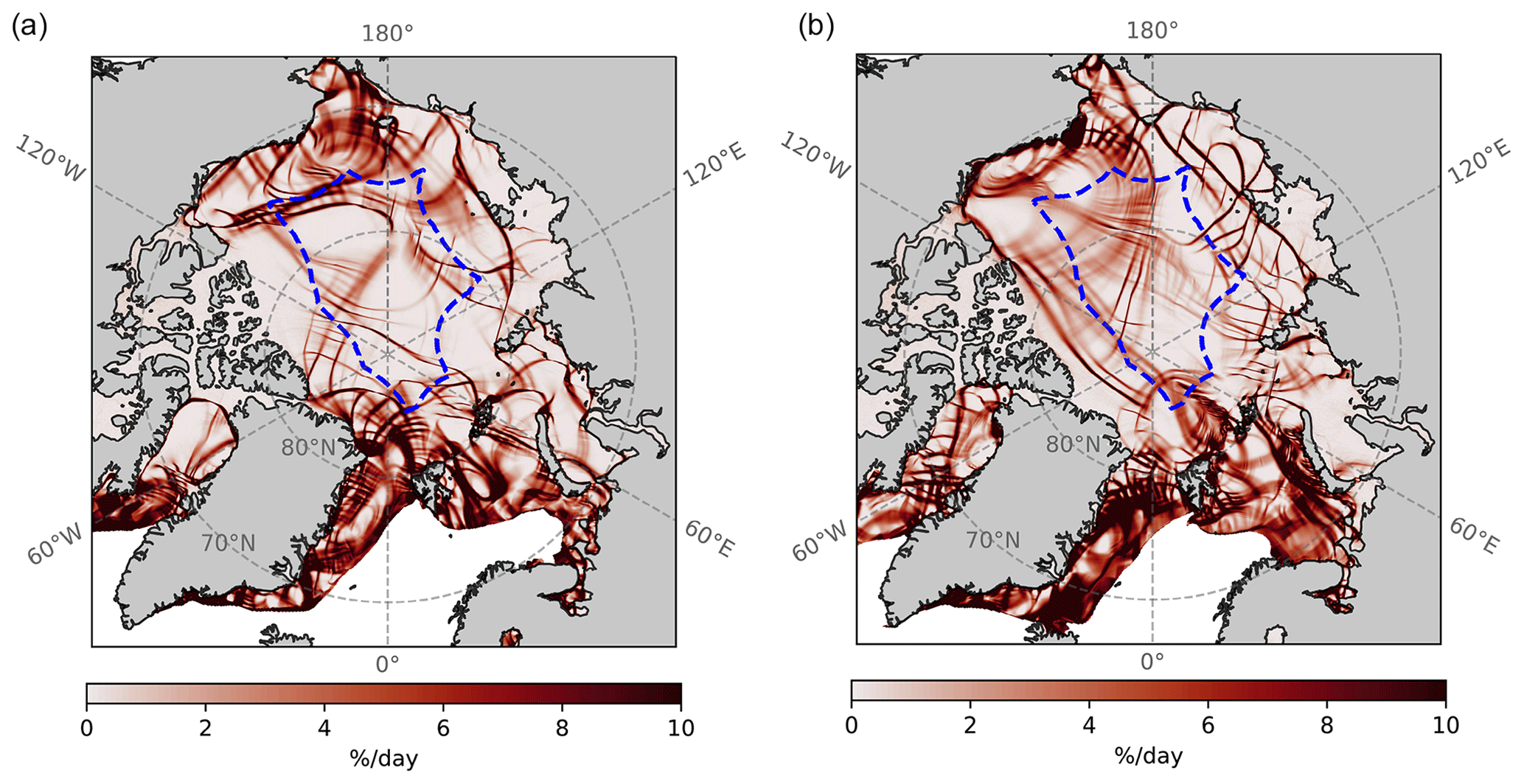
Figure 10 Daily-mean sea ice total deformation on 20 December (a) and 6 February (b) simulated by CESM and TS015. The region subjected to further scaling analysis is outlined by the dashed blue line in each panel.

3.3.2 Spatial scaling

We carry out spatial scaling analysis for two typical periods during the winter, focusing on four typical temporal scales: 1, 3, 10 and 30 d. Figures 11 and 12 show the results around 20 December and 6 February, respectively. At q=1 and 1 d scale, the spatial scalings of sea ice deformation are both very shallow: β=0.0623 and 0.121, respectively. This period of 2 d corresponds to different strengths and depths of the Beaufort High and slightly different Arctic Oscillation indices, and consequently the drift and deformation fields are distinct (see Figs. 6 and 11 of Xu et al., 2021). At different orders of momentum, the mean deformation rates all follow the power-law scaling. On higher orders (q>1), large deformation events are more dominant in the mean deformation rate, corresponding to steeper scaling (i.e., larger values of β). Furthermore, the value of β grows nonlinearly with q. With the increase in the moment order, the deformation rate decreases faster with respect to the increase in the spatial scale (L). Correspondingly, the convex shape of β(q) indicates that the model simulates multi-fractal sea ice deformation.

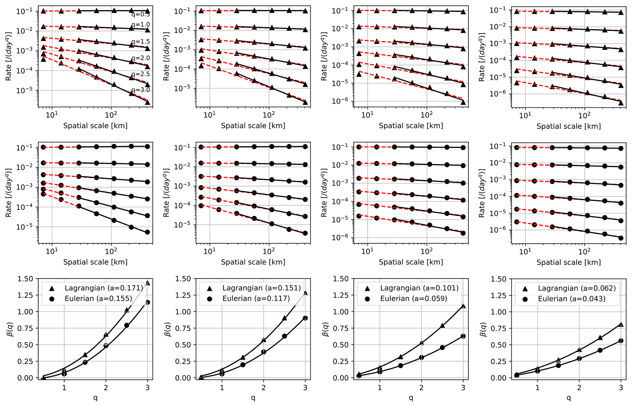
For the period of study surrounding 20 December, at larger temporal scales from 1 to 30 d, the average deformation rates decrease at all spatial scales and moments of order. More importantly, the value and the shape of β(q) also change significantly with the temporal scale. At q=1 and the 1 d temporal scale, the value of β is 0.0623. For larger temporal scales, the mean deformation rate gradually decreases, which also applies to the structure function of β. In particular, the convexity of β(q), indicated by the fitted value of a, decreases drastically from 0.137 (1 d) to 0.064 (30 d). The change in a indicates that there is a strong coupling between the spatial and temporal domain for the sea ice deformation. Similar results hold for the period around 6 February, with the two following major differences: (1) a more convex β(q) around 6 February than 20 December and (2) a faster decrease in a with respect to T (i.e., the temporal scale). The most significant drop in a occurred from the 3 to the 10 d scale for 6 February (from 0.151 to 0.101). For comparison, that for 20 December is between 10 and 30 d (from 0.093 to 0.064). Regarding the differences between the two periods, we conjecture that the process-dependent deformations are the major cause, including the strength of the spatial–temporal coupling. Further analysis is needed for the attribution of these differences to various factors, including the sea ice status, its deformation history and the forcings.

For comparison, we also show the results based on Eulerian deformation fields in both Figs. 11 and 12, including the power-law fittings and the structure functions of β(q). The method details are introduced in Appendix B. For both periods of study, the scaling analysis using Lagrangian tracking results shows steeper β functions with higher convexity across all temporal scales (i.e., larger values of a). For 6 February, the difference between the two is more pronounced. Note that the scaling analysis should be carried out based on the Lagrangian perspective. The objective of the comparisons is to demonstrate that there are systematic differences in the scaling analysis when using the Eulerian model outputs. The quantitative differences in the deformation rates may arise from (1) the deformation events being misaligned between the Eulerian and the Lagrangian perspectives and (2) the secondary effect of changing shapes and scales when the sea ice deforms within the Lagrangian perspective, which is not captured by the Eulerian framework.

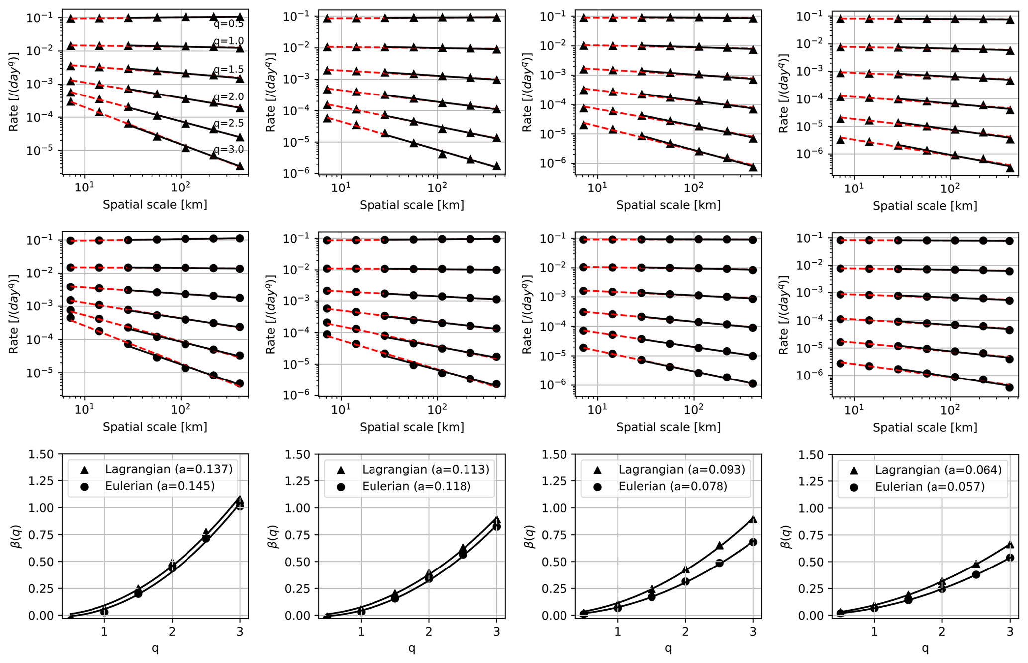
Figure 11 Spatial scaling around 20 December. Four temporal scales are evaluated: 1 d (first column), 3 d (second column), 10 d (third column) and 30 d (last column). Results with Lagrangian tracking (triangles) are compared with those based on temporal mean Eulerian deformation fields (dots). Black lines in each panel represent the fittings with the spatial scale of 30 km and coarser, and dashed red lines represent the fittings with the whole resolution range of TS015 (7.3 km and coarser). The fitted parameter of a for the structure function β(q) is shown in the legend.

Figure 12 Same as Fig. 11 but for 6 February.

3.3.3 Temporal scaling and spatial–temporal coupling

For the temporal scaling analysis, we focus on the spatial scale of the model's effective resolution (L=22 km). Figure 13 shows the results for the outlined region in Fig. 10 in the month of December (left) and February (right). The analyzed temporal scale is in the range between 1 and 30 d. Similar to the spatial scaling results, the power-law scaling is witnessed for the temporal scaling (top panels of Fig. 13). Also, convex structure functions of α(q) are present for both months, with the fitted value of c as 0.063 and 0.059, respectively. These results indicate that the model also simulates multi-fractal sea ice deformation in the temporal domain.

Evidently, the power-law scaling at sub-daily scales is much shallower than that between 1 and 30 d. Similar behavior of the sea ice is observed in Oikkonen et al. (2017), which covers the temporal scale from about 10 min. We consider the shallower scaling in the simulations to be qualitatively consistent with the observation. However, although the model's dynamics time step is sufficiently short (see Appendix A), the temporal resolution of the forcing dataset is much coarser, at 6-hourly. In order to fully study the simulation of the sub-daily sea ice deformation, we need high-frequency forcing datasets or the coupled simulation with the high-resolution interactive atmospheric component (Zhang et al., 2023).

Similar to the analysis in Sect. 3.3.2, we also compute the temporal-mean Eulerian deformation fields and the equivalent scaling analysis. Since we only output daily model fields, the analysis is limited to the temporal scale between 1 and 30 d (middle row of Fig. 13). Apparent power-law scaling is witnessed for both months. However, the structure function of α(q) with the Lagrangian tracking is systematically less convex than that based on Eulerian fields, with lower values of c for both months (bottom row of Fig. 13). This result, together with that in Sect. 3.3.2, shows that the scaling analysis should be carried out in the Lagrangian framework. Although the scaling analysis with the model's Eulerian mean fields yields apparent multi-fractal sea ice deformation, the results are systematically different from those based on the Lagrangian analysis.

Furthermore, we conduct the initial analysis of the spatial–temporal coupling during the whole winter (December to March). For the region of study (outlined in Fig. 10), we utilize all of the Lagrangian tracking results by forming and tracking Lagrangian patches at various spatial and temporal scales. Specifically, for each combination of the spatial and the temporal scale (i.e., L and T), we form Lagrangian patches that satisfy the following criteria: (1) they start at interleaved Eulerian grid locations separated by $L/\mathrm{2}$ in both directions, and (2) the time difference between their starting time and 0:00 of 1 December is separated by $n\cdot T/\mathrm{2}$, where $n\in \mathit{\{}\mathrm{0},\mathrm{1},\mathrm{2},\mathrm{3},\mathrm{\dots }\mathit{\}}$. With these two criteria, we in effect split the Lagrangian tracking results into sea ice Lagrangian patches with 50 % temporal and spatial overlapping. As a result, not only do we attain full coverage of the study area/period, but also we avoid potential sampling issues associated with the changing weather regimes.

The relationship between the curvature parameter of the spatial (temporal) scaling structure function and the temporal (spatial) scale is shown in Fig. 14a (b). There is evident coupling between the spatial domain and the temporal domain, with decreased curvature of the spatial (temporal) structure function at larger temporal (spatial) scales. In particular, for the temporal scaling, there is a good fit of the curvature parameter c to the power law (Fig. 14b), which is consistent with various estimations based on in situ and satellite-based remote sensing observations (Rampal et al., 2008; Marsan and Weiss, 2010). However, for the spatial scaling, the relationship of a to the temporal scale is much flatter and, in particular, less convex for a power-law fit (Fig. 14a). We note that during different periods of the winter, the sea ice drift and deformation patterns are highly heterogeneous (due to changing weather), with the sea ice conditions undergoing significant changes. For example, the spatial scaling exponent shows large temporal variability (Rampal et al., 2019) and is likely linked to the atmospheric forcing patterns (Xu et al., 2021). Therefore, we adopt another fitting with the log-quadratic form: $y=p\cdot \log (x{)}^{\mathrm{2}}+q$. This new form yields a much higher fitting to the relationship between the curvature parameter a and the temporal scale T (R² from 0.882 to 0.989). The efficacy of the power-law fitting, as well as the full analysis of the spatial–temporal coupling as simulated by CICE, is beyond the scope of this study. In particular, the sensitivity to the sea ice rheology model and other dynamic processes is planned for both CICE on its own and coupled experiments with CESM.

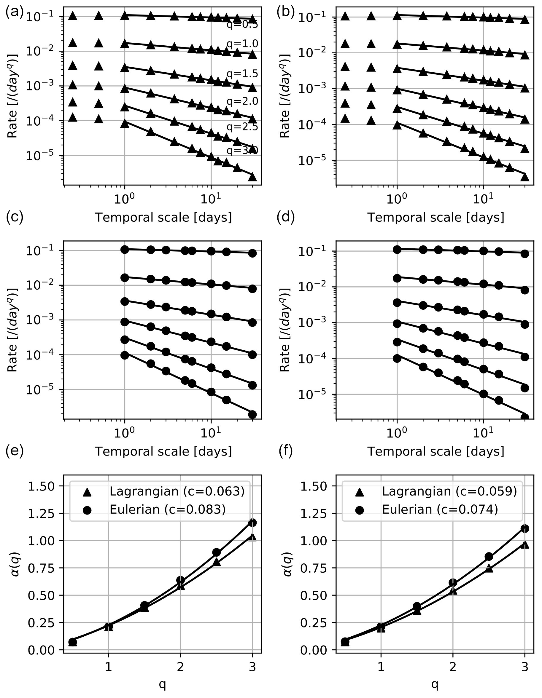
Figure 13 Temporal scaling for December (a, c, e) and February (b, d, f) at the spatial scale of 22 km (i.e., 3× the original grid resolution). Similar to Figs. 11 and 12, the results with Lagrangian tracking and Eulerian mean deformation fields are shown by triangles and dots, respectively. Note that the fittings are only computed for 1 d or coarser temporal scales (indicated by the abscissa range of the fitted lines).

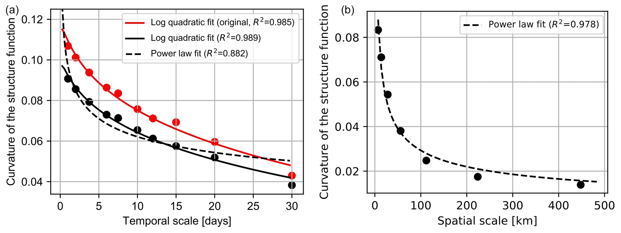
Figure 14 Temporal–spatial coupling (December–March) analysis of Lagrangian tracking deformation fields: the curvature of the structure function of the spatial scaling exponent as a function of temporal scale is shown in panel (a), and the curvature of the structure function of the temporal scaling exponent as a function of spatial scale is shown in (b). The solid and dashed lines represent the logarithm-quadratic fitting of $y=p\cdot \left(\log \right(x){)}^{\mathrm{2}}+q$ and the power-law fitting of $y=p\cdot x^q$, respectively. The red (black) line in the first panel shows the fitting with all the spatial scales (the scales with the model's effective resolutions). The R² values of each fitting are shown at the top of each panel.

4 Summary and discussion

We design and implement the online Lagrangian tracking in the sea ice model of CICE. It is incorporated in the dynamics process of CICE and fully supports the domain decomposition and parallel computing in CICE. Compared with the common practice of offline sea ice tracking (Bouchat et al., 2022; Sumata et al., 2023), the online tracking has several advantages. First, the offline tracking usually requires the storage of high-frequency sea ice drift data, which is not needed for the online tracking. Second, since the online tracking is carried out per dynamics step, the tracking error is minimal. For offline tracking, the tracking uncertainty arises from the relatively coarse temporal-mean (e.g., daily) sea ice drift fields, as well as the variable tracking frequency (see examples in Bouchat et al., 2022). Moreover, the study of sea ice dynamics at small temporal scales (such as sub-daily motions) with offline tracking requires an even finer resolution of the stored sea ice drift. The study of these processes is readily supported by the online tracking (see Fig. 13 and also Oikkonen et al., 2017). Computationally, the Lagrangian tracking only induces a small overhead to the overall simulation. For example, for the daily deployment of Lagrangian points in the 7 km experiment in Sect. 3, there are on average 30 to 35 million active Lagrangian points, and the extra computational overhead is less than 3 %. Therefore, the current implementation is capable of supporting high-resolution simulations with a large quantity of Lagrangian points.

In Sect. 3.3 we carried out the spatial and the temporal scaling analysis with the Lagrangian tracking based on high-resolution simulation during winter. As shown, the CICE model simulates multi-fractal sea ice deformation fields both spatially and temporally; it also simulates the tight coupling between the spatial and the temporal domain. The scaling properties of the simulations are consistent with observed statistics based on high-resolution synthetic aperture radar satellite payloads. In particular, we compare the Lagrangian-based scaling statistics with the counterparts based on Eulerian model outputs. Results highlight the importance of using Lagrangian-based diagnosis for the scaling analysis: although the analysis based on Eulerian output also yields convex structure functions, the fitted convexity parameters are significantly different from those based on the Lagrangian perspective.

In order to compare with the observed sea ice drift and deformation (e.g., RGPS) as well as the scaling statistics, we plan to carry out high-resolution, atmospherically forced historical simulations with the CICE model or CESM assisted with the Lagrangian tracking. Consequently, fine tuning of the sea ice model parameters is needed for (1) the optimization of the simulation of various sea ice parameters such as sea ice thickness and (2) improved comparability to the observed sea ice deformation. In particular, in Bouchat and Tremblay (2020), the authors proposed a new estimation of deformation rates regarding their uncertainties. Better consistency with model simulations is attained with further incorporation of the model simulation and tracking uncertainties (Bouchat et al., 2022). We plan to incorporate the method and carry out a systematic evaluation of the model's capability to simulate the observed multi-scale sea ice deformation. In particular, the sensitivity to the sea ice rheology is a key aspect of the planned future work (Tsamados et al., 2013; Bouchat et al., 2022).

In this first version of the Lagrangian tracking in CICE, virtual buoys are supported, which can be deployed at regular time intervals and in regular locations. Section 3.2 shows that with the pairing between the physical buoys and the respective virtual buoys, the simulated tracks are generally consistent with observations. For future development, we plan to support the deployment of physical buoys in the simulation at prescribed times and locations so that we can make better comparisons with observational datasets such as IABP. Moreover, key Lagrangian-tracking-related parameters (in Appendix B) are planned to be configured through a subset of the namelist in the future development plan. Finally, the current design of Lagrangian tracking is based on the Arakawa-B grid sea ice dynamics and the transport remapping scheme. For the compatibility with ongoing development in CICE6 (https://github.com/CICE-Consortium/CICE/releases, last access: 8 September 2024), we also plan to incorporate flux-form-based Lagrangian tracking, which is suitable for Arakawa-C grid sea ice dynamics (Lemieux et al., 2024).

The Lagrangian tracking can be used for a variety of science questions and applications related to sea ice. Large-scale Lagrangian surveys can be carried out in the simulations, complementary to buoys' measurements, which are limited in terms of spatial and temporal coverage. For example, virtual buoys can be deployed in historical simulations, which enables the systematic study of the thermodynamic and dynamic history of the sea ice (Sumata et al., 2023). Furthermore, CICE is widely adopted for the high-resolution sea ice operational systems (Smith et al., 2016; Yang et al., 2020). The online tracking of sea ice in key regions can be carried out for sea ice forecasts, in order to support operations and ship navigation in polar waters.

Appendix A: Model configuration and parameters of CICE

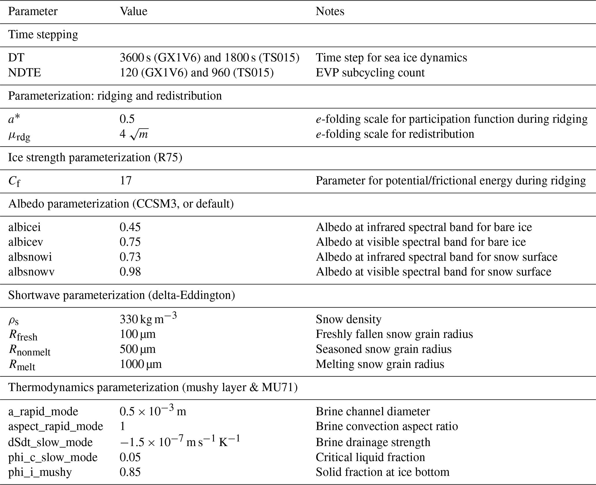
CICE (version 5.0) is configured with five discretized thickness categories for the ice thickness distribution (ITD) and eight and three layers for sea ice and its snow cover, respectively. The elastic–viscous–plastic (EVP) rheology model is used for all experiments. The ice strength parameterization follows that in Rothrock (1975), which relates the ice strength to the gain of the potential energy during the ridging process. The ridging–rafting parameterization uses an exponential distribution form of the ridged ice in the ITD. For sea ice thermodynamics, the mushy-layer physics parameterization is adopted (Turner et al., 2013). The delta-Eddington (D-E) scheme is used for the radiation processes (Holland et al., 2012). Table A1 lists the key parameters of the model. The parameters are the same across all numerical experiments by default, except the dynamics time step and the EVP sub-cycling count (NDTE, number of time steps (DT) for the elastic waves). These two parameters are set differently between the experiments with GX1V6 and those with TS015. The shorter time step is adopted for TS015 to ensure numerical stability, and the value of NDTE is further enlarged for the numerical convergence of the EVP rheology (Lemieux et al., 2010; Xu et al., 2021).

Table A1 Major model parameters of CICE.

Appendix B: Scaling analysis with Lagrangian tracking and Eulerian fields

We carry out the scaling analysis of the sea ice deformation at various spatial and temporal scales (Rampal et al., 2019; Bouchat and Tremblay, 2020). The Lagrangian tracking results, as well as the model outputs on Eulerian grids, are used to compute the mean sea ice deformation rates at the corresponding scales. A set of Lagrangian points form an enclosed Lagrangian patch, for which we compute the spatial derivatives of velocities (i.e., u_x, u_y, v_x and v_y) as follows:

$$\begin{array}{ll}{\displaystyle }& {\displaystyle }{u}_x={\displaystyle \frac{\mathrm{1}}{A}}\oint u\text{d}y\\ {\displaystyle }& {\displaystyle }{u}_y=-{\displaystyle \frac{\mathrm{1}}{A}}\oint u\text{d}x\\ {\displaystyle }& {\displaystyle }{v}_x={\displaystyle \frac{\mathrm{1}}{A}}\oint v\text{d}y\\ \text{(B1)}& {\displaystyle }& {\displaystyle }{v}_y=-{\displaystyle \frac{\mathrm{1}}{A}}\oint v\text{d}x.\end{array}$$

These derivatives are used to compute the deformation rates as in Eqs. (2) to (3). The line integral in Eqs. (B1) is carried out over the Lagrangian patch that originally covers a regular rectangular domain. Then each point on the patch's outer boundary, called a vertex, has its location of $(x_i^j,y_i^j)$ at the time of t_j and the new location of $(x_i^{j+\mathrm{1}},y_i^{j+\mathrm{1}})$ at the time of t_j+1. Figure B1 shows the schematics for a Lagrangian patch with four corner points. We can estimate its mean velocity (u_i,v_i) as the ratios of the displacements to the time difference: $\left(x_i^{j+\mathrm{1}}\mathrm{-}{x}_i^j\right)/(t_{j+\mathrm{1}}-t_j)$ and $\left(y_i^{j+\mathrm{1}}\mathrm{-}{y}_i^j\right)/(t_{j+\mathrm{1}}-t_j)$. Furthermore, in order to compute the line integrals at time t, we compute the mean velocity on each edge as follows (for the example in Fig. B1):

$$\begin{array}{}\text{(B2)}& u_x={\displaystyle \frac{\mathrm{1}}{A}}\sum _{i=\mathrm{1}}^{\mathrm{4}}{\displaystyle \frac{\mathrm{1}}{\mathrm{2}}}\left(u_{i+\mathrm{1}}+u_i\right)\left(y_{i+\mathrm{1}}-y_i\right),\end{array}$$

where A is the area the set of Lagrangian points covers:

$$\begin{array}{}\text{(B3)}& A={\displaystyle \frac{\mathrm{1}}{\mathrm{2}}}\sum _{i=\mathrm{1}}^{\mathrm{4}}\left(x_i{y}_{i+\mathrm{1}}-x_{i+\mathrm{1}}{y}_i\right).\end{array}$$

In order to complete the line integral, we set x₅=x₁ and, similarly, the corresponding values of y₅, u₅ and v₅. For larger spatial scales, we start with a larger set of Lagrangian points that have their original locations on the Eulerian grid locations and cover a locally rectangular area. Then, the velocities, their spatial derivatives and the line integrals are computed, followed by the computation of the deformation rates. This is equivalent to the aggregation of all the smallest rectangular units of four Lagrangian points that constitute the whole rectangular area. Note that at the beginning of each model day, we deploy the Lagrangian points on all Eulerian grid locations, so that we attain full spatial and temporal coverage, from the daily scale and above. Additionally, we further exclude the cases with the size change by a factor of 2 or larger.

For comparison, we also compute the equivalent deformation rates based on Eulerian fields. We directly obtain the temporally mean velocities on each Eulerian grid location and compute the velocity gradients correspondingly (Fig. B1b). Different spatial scales correspond to the various areas that are associated with different rectangular grid cells, which do not change throughout the simulation.

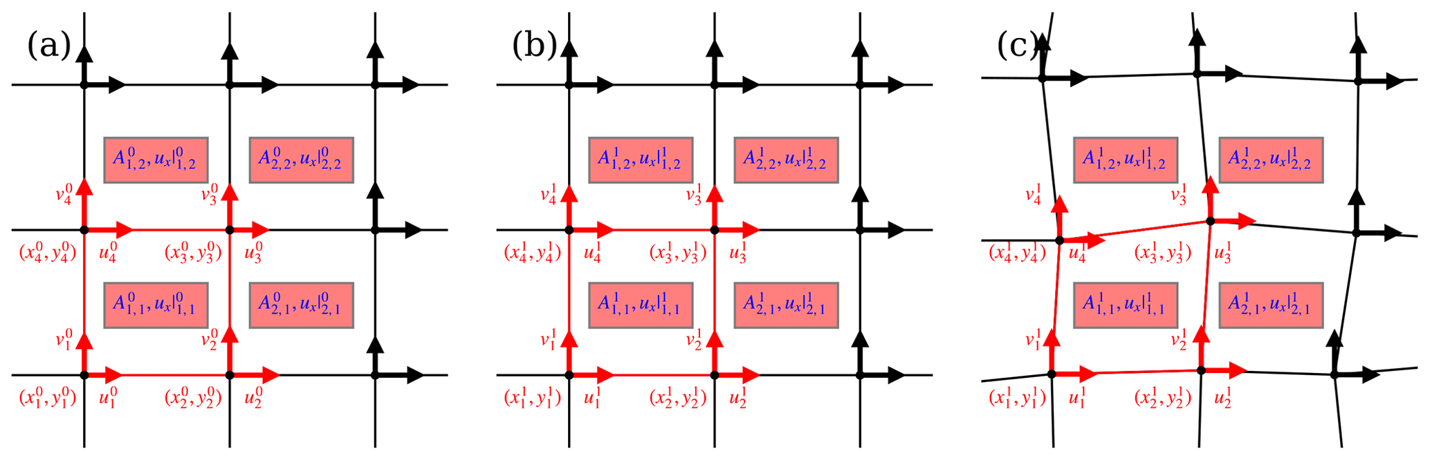
Figure B1 Schematics of the scaling analysis with Lagrangian tracking and the equivalent Eulerian model outputs. The locations of Eulerian and Lagrangian points at the initial time t₀ are shown in panel (a), and those at time t₁ are shown in panel (b) and (c), respectively. The spatial scale L is defined as the square root A, which is the area of the region covered by the four Lagrangian/Eulerian points. Note that in our analysis, the initial locations of the Lagrangian points are the regular, Eulerian grid points. For comparison, on the same timescale (i.e., $T=t_{\mathrm{1}}-t_{\mathrm{0}}$), we compute the model-output mean velocities on the Eulerian grid points, as well as the displacement-based velocity estimations for Lagrangian points.

For both Lagrangian statistics and the Eulerian counterparts, we only compute the deformation field that is contained by the areas covered at the coarsest spatial scale. This practice ensures that there is no preferential sampling of the deformation events.

A wide range of both spatial and temporal scales are adopted for the computation of the deformation rates. The statistics of $\dot{\mathit{ϵ}}(T,L)$, which is the deformation rate at the spatial scale of L and the temporal scale of T, include its qth order (i.e., ${\dot{\mathit{ϵ}}}^q(T,L)$), and the mean values are computed over the studied area. It is worth noting that the spatial scale of L varies within the studied domain, as well as with time for the Lagrangian tracking. Therefore, both the mean value of ${\dot{\mathit{ϵ}}}^q(T,L)$'s and that of the spatial scales of L's are used for the scaling analysis.

Appendix C: Major parameters of Lagrangian tracking

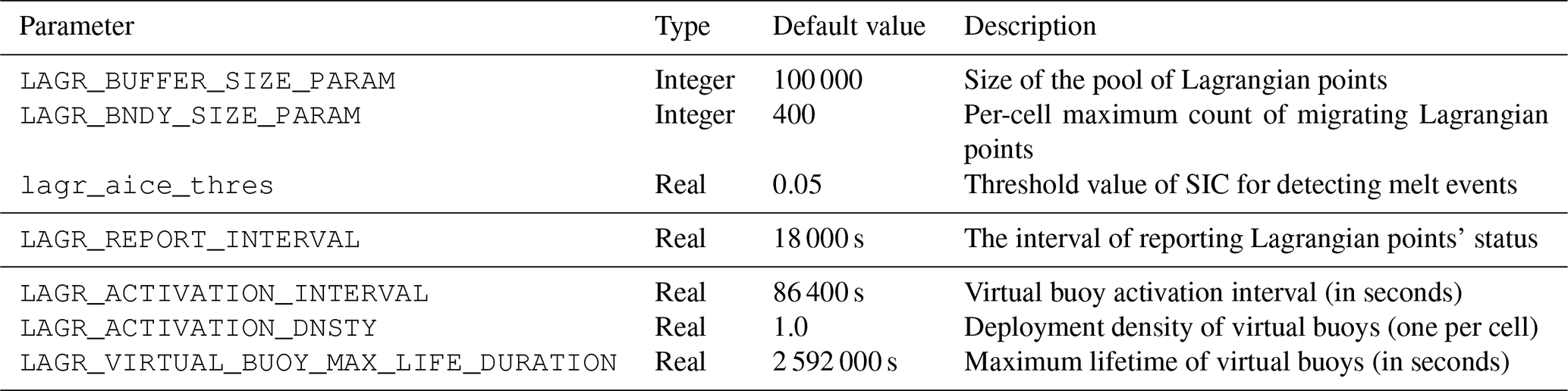
Table C1 shows the major user-specified parameters for running the Lagrangian tracking in CICE. In the current implementation, they are configured at the compile time of the model. In the future, we plan to implement certain parameters to be configurable through the namelist.

Table C1 User-prescribed parameters of Lagrangian tracking.