the Creative Commons Attribution 4.0 License.
the Creative Commons Attribution 4.0 License.
 | 12 Sep 2024
Preliminary evaluation of the effect of electro-coalescence with conducting sphere approximation on the formation of warm cumulus clouds using SCALE-SDM version 0.2.5–2.3.0
Ruyi Zhang
Limin Zhou
Shin-ichiro Shima
Huawei Yang
The phenomenon of electric fields applied to droplets, inducing droplet coalescence, is called the electro-coalescence effect. An analytic expression for electro-coalescence with the accurate electrostatic force for a pair of droplets with opposite-sign charges is established by treating the droplets as conducting spheres (CSs). To investigate this effect, we applied a weak electric field to a cumulus cloud using a cloud model that employs the super-droplet method, a probabilistic particle-based microphysics method. This study employs a two-dimensional (2D) large-eddy simulation (LES) in a flow-coupled model to examine aerosol microphysics (such as collision–coalescence enhancement, velocity fluctuations, and supersaturation fluctuations) in warm cumulus clouds without relying on subgrid dynamics. In the simulation, we assume that droplets carry opposite-sign charges and are well mixed within the cloud. The charge is not treated as an individual particle attribute. To assess fluctuation effects, we conducted 50 simulations with varying pseudo-random number sequences for each electro-coalescence treatment. The results show that, with CS treatment, the electrostatic force contributes a larger effect on cloud evolution than in previous research. With a lower charge limit of the maximum charge amount on the droplet, the domain total precipitation with CS treatment for droplets with opposite signs is higher than that with the no-charge (NC) setting. Compared to previous work, the multi-image dipole treatment of CS results in higher precipitation. It is found that the electro-coalescence effect could affect rain formation even when the droplet charge is at the lower charge limit. High pollution levels result in greater sensitivity to electro-coalescence. The results show that, when the charge ratio between two droplets is over 100, the short-range attractive electric force due to the multi-image dipole would also significantly enhance precipitation for the cumulus. It is indicated that, although the accurate treatment of the electrostatic force with the CS method would require 30 % longer computation time than before, it is worthwhile to include it in cloud, weather, and climate models.
- Article
(3015 KB) - Full-text XML
- BibTeX
- EndNote


Clouds are regarded as playing a key role in climate systems, and the collision–coalescence of cloud droplets plays a key role in rain formation. Droplet coalescence is one of the main processes leading to precipitation, affecting cloud microphysics and thereby changing the global radiation budget (Pruppacher and Klett, 2010, Chap. 15; Grabowski and Wang, 2013; IPCC AR6 WG1 Ch7, 2021). Several studies have reported that the electrostatic force on charged droplets could significantly influence the droplet coalescence and droplet–aerosol coagulation in weakly electrified clouds (Rayleigh, 1879; Tinsley et al., 2001; Tinsley and Zhou, 2006; Zhou et al., 2009; Tripathi et al., 2008; Pruppacher and Klett, 2010; Zhang et al., 2018; Guo and Xue, 2021). This electrostatic-force-induced effect is called electro-coalescence or electro-anti-coalescence (Tinsley, 2008) and could even explain the link between solar wind fluctuations and changes in atmospheric parameters, such as cloud cover, polar surface pressure, and the effective radiation in polar regions (Kniveton et al., 2008; Lam et al., 2014; Frederick and Tinsley, 2018; Frederick et al., 2019).
In weakly electrified clouds, the accumulation of space charges on droplets is controlled by the diffusion of atmospheric ions produced by the cosmic ray flux, and the concentration is dependent on the ratio of attachment and recombination and the downward ionosphere–earth current density (Jz). When the Jz penetrates the cloud, the gradients of the electric field at the cloud boundary could generate net positively charged droplets at the upper cloud boundary and net negatively charged droplets at the lower boundary (Zhou and Tinsley, 2007; Nicoll and Harrison, 2016). The observations of Beard et al. (2004) revealed that, with a Jz of 1–6 pAm−2 in stratocumulus and altostratus clouds, a cloud droplet with the radius of 10 µm can accept approximately 100 elementary charges, which is consistent with the theoretical calculations by Zhou and Tinsley (2007). In cumulus clouds, vertical convection causes positively charged droplets from the upper boundary and negatively charged droplets from the lower boundary to mix, leading to electro-coalescence. The maximum charge on the droplets is determined by the air breakdown voltage for corona discharge (Meek and Craggs, 1954) and is a quadratic function of the droplet radius (Khain et al., 2004; Andronache, 2004).
Numerous studies have focused on parameterising the microphysics of the electro-coalescence of particles; the challenge is to approximate the calculation of the electrostatic force between charged droplets. In the 1970s, the collision efficiency of oppositely charged droplets evaluated with a centred Coulomb force (CB) indicated that only in strongly electrified clouds can the charge on droplets significantly affect cloud droplet coagulation (Wang et al., 1978). The trajectory simulation studies by Tinsley et al. (2001), Tinsley and Zhou (2006), Tripathi et al. (2006), and Zhou et al. (2009) revealed that, in a weakly electrified cloud, when taking into account the image charge force, the collision rate coefficient between the charged droplets could be different. Even with droplet charges of the same sign, the collision rate coefficient could be enhanced as a function of the charge on the particles with radii ranging from 0.1 to 10 µm (Zhou et al., 2009). The so-called Greenfield gap, identified by Greenfield (1957), describes the reduced concentrations of particles in the 0.1 to 1 µm size range. The Greenfield gap could be reduced with sufficient charging of the droplets. Simulation results showed that, for particles with radii smaller than 0.1 µm, when the particles obtain a large charge due to the evaporation of highly charged droplets, the collision rate coefficient is significantly decreased due to the repulsive electric force of droplets with charges of the same sign and is increased for charges of the opposite sign (Tinsley and Leddon, 2013). The updated simulation by Zhou et al. (2009), with an exact electric force treatment with the conducting sphere (CS) method, indicated that the collision efficiency is a factor of 2 higher in the Greenfield gap than in the results of a single image charge (IM) treatment. A few laboratory experiment results were consistent with these theoretical simulations (Ardon-Dryer et al., 2015). These findings highlight the need to represent coagulation due to droplet and aerosol charges in the cloud model. Khain et al. (2004) (hereafter Khain04) conducted a zero-dimensional simulation to study the effect of seeding charged droplets on a cumulus cloud using the spectral-bin cloud model with a four-dimensional (mass and charging rate of two droplets) collision efficiency lookup table based on the static electric force between charged droplets. The results showed a significant response in the evolution of clouds due to charged droplets. Khain04 set a charging rate equal to 5 % of the maximum charge of natural droplets, which is 2.5 times larger than the values reported by Zhou and Tinsley (2007), to study electro-coalescence impact on rain enhancement and fog elimination. Andronache (2004) and Wang et al. (2015) claimed that charged droplets significantly contribute to below-cloud scavenging according to the analytical formula suggested by Davenport and Peters (1978), where the minimum amount of charge on droplets is 7 % of the maximum limit. However, only CB treatment was used in the Andronache (2004) and Wang et al. (2015) simulations.
Lagrangian particle-based approaches create more accurate solutions for the collision–coalescence process compared to bin microphysics schemes, as they overcome the limitations imposed by the assumptions of bin schemes (Grabowski et al., 2019; Liu et al., 2023). In this study, we estimate the effect of electro-coalescence from Jz on warm cumulus clouds by an exact treatment of electric forces using the CS method, using the super-droplet method (SDM), a Lagrangian particle-based cloud microphysics scheme. The lower charging rate threshold for electro-coalescence is discussed. The extreme assumption of the droplet-charging scenario of opposite-sign charge is investigated. The electro-anti-coalescence (Tinsley and Zhou, 2015) between charged droplets and particles could also be important for deep convection and stratus cloud evolution.
In this study, we assume that the charged droplets are well-mixed in the warm cumulus cloud and focus on the electro-coalescence effect. A Lagrangian particle-based cloud model is used with the particle-size-resolved treatment following the SDM by Shima et al. (2009, 2020). Compared to bin microphysics schemes, the SDM eliminates numerical diffusion and provides more accurate solutions for well-mixed volumes (Grabowski et al., 2019). Despite its sensitivity to super-droplet initialisation and a higher variance than observed in reality (Liu et al., 2023), the SDM is well-suited for this study. This section provides a description of the SDM, how we generalise the exact electric force treatment with the CS method approach for the cloud model, and the numerical simulation setup.
2.1 Definition of super-droplets
Super-droplets have been defined in detail by Shima et al. (2009, 2020). A super-droplet represents multiple droplets with the same attributes and position, and this multiplicity is denoted by the positive integer ξi(t), which can be different in each super-droplet and is time-dependent due to the definition of coalescence. Then, each super-droplet has its own position xi(t) and its own attributes ai(t) that characterise the ξi(t) identical droplets represented by super-droplet i. In this study, we assume that the attributes consist of the equivalent radius and the mass in the droplet . Since each real droplet takes different positions and attributes, a super-droplet is a kind of coarse-grained view of droplets both in real space and in attribute space. Assume that Ns(t) is the number of super-droplets in the domain at time t. Then, the super-droplets represent real droplets in total.
2.2 Motion of a super-droplet
The advection and sedimentation processes were described in detail by Shima et al. (2009, 2020) as follows:
where is the mass of droplet i and ρliq=1.0 g cm−3 is the density of liquid water. is the drag force from moist air, g is the gravity of Earth, and is the unit vector in the direction of the z axis. gives the reaction force acting on the moist air (Montero-Martínez et al., 2009). Considering that the relaxation to the terminal velocity is instantaneous, the equation of motion becomes
where Ui=U(x) is the ambient wind velocity of the ith particle and is the terminal velocity, which in general is a function of the attributes ai and the state of the ambient air.
The motion of a super-droplet is the same as that of a droplet, which is described in Eq. (2), and vt(t) is equal to the terminal velocity.
2.3 Condensation and evaporation
The condensation/evaporation process is based on Köhler's theory, which takes into account the solution and curvature effects on the droplet's equilibrium vapour pressure (Köhler, 1936; Rogers and Yau, 1989; Pruppacher and Klett, 2010, Chap. 13). The growth equation of radius Ri is derived as follows:
where S is the ambient saturation ratio, Fk represents the thermodynamic term associated with the latent heat release, and Fd represents the term associated with vapour diffusion. The term represents the curvature effect, which expresses the increase in the saturation ratio over a droplet compared with that of a plane surface. The term represents the reduction in the vapour pressure due to the presence of a dissolved substance, where b depends on the mass of solute Mi dissolved in the droplet. cm K T−1, and b≃4.3 cm3. In , T is the temperature, i≃2 is the degree of ionic dissociation, and ms is the molecular weight of the solute. Rv is the individual gas constant for water vapour, K is the coefficient of thermal conductivity of air, D is the molecular diffusion coefficient, L is the latent heat of vaporisation, and es(T) is the saturation vapour pressure. Note that the charge-induced reduction in surface tension decreases the equilibrium vapour pressure (Weon and Je, 2010).
2.4 Collision–coalescence and the electric effect
In warm clouds, the collision–coalescence of two droplets to form a larger droplet is responsible for precipitation and cloud lifetime. The droplet growth due to the coalescence is controlled by the net action of various forces impacting the relative motion of the two droplets. The effective collision–coalescence of droplets can be evaluated by the collision–coalescence kernel K, which can be described as follows:
where is the collision–coalescence efficiency and KB is the Brownian coagulation kernel. R represents the radius of the larger droplet, and r is the radius of smaller droplets of the given pair (R,r). Similarly, QR represents the charge of larger droplets, and qr is the charge of smaller droplets. vR represents the terminal velocity of larger droplets, and vr is the terminal velocity of smaller droplets. In this study, we assume E0(R,r) takes into account the effect of a small droplet/particle being swept by the stream flow around a larger droplet or bouncing on the surface by front, side, or rear collection, or droplets of similar size collide on the downstream side and are caught (Davis, 1972; Hall, 1980; Jonas, 1972; Pruppacher and Klett, 2010, Chap. 14). Following Seeßelberg et al. (1996) and Bott (1998), the collision efficiency of Davis (1972) and Jonas (1972) for small droplets and the collision efficiency of Hall (1980) for large droplets are adopted. We assume the coalescence efficiency is unity in this study.
The Brownian coagulation kernel KB is given by Seinfeld and Pandis (2006, Chap. 13) using the correction factor of Fuchs (1964) to correct the boundary condition of the surface of absorbing particles. The Fuchs form of the Brownian coagulation coefficient is derived as follows:
where
ℓi represents the particle mean free path, Di represents Brownian diffusivity, Dpi represents diameters of particles, mi is the particle mass, J K−1 is the Boltzmann constant, μ represents the dynamic viscosity of air, and Cc is a slip-correction factor.
Referring to Andronache (2004), we propose a parameterisation of the collision efficiency due to the electric force based on the work by Zhou et al. (2009) and Tinsley and Zhou (2015). The induced charge on the droplet is involved in our Ees. Based on the trajectory model simulation, the electric force with the IM treatment (Tinsley and Zhou, 2006) and the CS treatment (Zhou et al., 2009) can significantly contribute to the collision efficiency. For droplets with opposite-sign charges, in the front and side collision ranges, the short-range attractive electric force due to the induced image charge provides additional force to balance the repulsive force. In the rear collision range, this short-range attractive force contributes to balancing the inertia. The rear collision range is relevant for droplets smaller than 0.1 µm: the droplets typically accept less than 1 elementary charge, meaning the electric force does not significantly impact the collision process. Therefore, the main electric force remains in the side and front collision range and droplets accept more than 1 elementary charge in this study.
The analytical parameterisation for the collision efficiency with the electric force suggested by Davenport and Peters (1978) is used with modification to include the image charge effect of oppositely charged droplets in our study. Tinsley and Zhou (2015) developed a charge effect for droplets with the same charge:
where cf is the Cunningham correction factor, v is the terminal velocity of the droplet, and Fes is the electric force between the colliding droplets.
In this study, Fes is calculated in four different ways, namely CB, IM, Khain04, and CS, which are given by Eqs. (13)–(16), respectively.
CB treatment considers only the Coulomb force between the centre points of the droplets. Then, Fes is given by
where F m−1 is the dielectric permittivity of free space. QR and qr are the charges of large and small particles. Rb is the distance between the centre of two droplets.
Khain04 used the superposition method to calculate a four-dimensional (with respect to droplet size and charge) lookup table for collision efficiency and present an approximated solution for the electrostatic forces of droplets with the following formula:
R and r represent the radii of the larger and smaller droplet in a pair of droplets. Note that, in this study, we calculate the collision–coalescence kernel of the Khain04 method with Eq. (13) for electrostatic forces and with Eq. (11) for the charge effect, whereas Khain04 used a four-dimensional lookup table for collision efficiency.
The distance parameter rnt is needed to calculate Fes of the IM and CS treatment. Based on the trajectory simulation results by Zhou et al. (2009), rnt is fitted as follows:
where rref=0.01.
When the large-droplet radius is 100 times larger than the small-droplet radius, the IM treatment is accurate enough. Fes for the IM treatment is given by
where (in N m2 C−2).
If the ratio between the droplet and the particle is less than 100, the electric force is treated by the CS method according to Zhou et al. (2009), which originates from Davis (1964):
where F5,F6, and F7 are dimensionless complex polynomial expressions given by Davis (1964) that depend only on the radii of the two droplets and their distance parameter rnt.
In this study, we assume that Jz charges the droplets. Zhou and Tinsley (2012) observed that droplets with a 10 µm radius achieve 70 % of their charge in 680 s. However, following the Andronache (2004) simplification of the complex charging process, we assume that the charge on droplets resulting from collision–coalescence reaches equilibrium instantaneously. We also consider an extreme scenario where the charge polarity of two colliding droplets is always opposite. The assumption of instantaneous charging might lead to an overestimation of the electro-coalescence effect. Regarding the charge polarity, convective mixing within cumulus clouds introduces oppositely charged droplets from the cloud boundary into the cloud interior. These droplets retain their opposite charges due to the relatively long discharge timescale, significantly impacting the early stages of raindrop formation. The coalescence of large rain droplets is dominated by gravity settling. Notably, Khain et al. (2004) addressed charge differences by subtracting the charge of opposite-polarity particles and adding the charge of same-polarity particles after collision–coalescence.
The voltage near a charged spherical particle is described by (Bleaney and Bleaney, 1993). The air breakdown voltage, V m−1, determines the maximum charge that cloud droplets can carry (Meek and Craggs, 1954). Consequently, the maximum charge that droplets can carry is as follows:
To simulate droplets in a weak electric field, we followed Andronache (2004) and described the mean charges on the larger and smaller droplets in a pair as a function of their radii as follows:
Here, is 2 orders of magnitude smaller than the maximum particle charge, representing weak-charge conditions, and the charging rate α is an empirical parameter (α is referred to herein as the droplet-charging rate) that varies between 0, which represents neutral particles, and 7, which represents highly electrified clouds associated with thunderstorms (Andronache, 2004). In our work, the α value ranges from 0.1 to 0.6, which represents a weakly electrified cloud. Compared with the maximum charge of the droplet method used by Khain04, when α ranges from 0.1 to 0.6 cm−2, the charge on the droplet reaches 0.3 % up to 2 % of the maximum charge, which is 10 times to 2 times smaller than the lowest value used by Khain04 and Wang et al. (2015). The minimum limit for the droplet charge is equivalent to 1 elementary charge. This could be a reliable estimation for the accumulated charge on droplets with the downward current density (Jz), since a droplet with a radius of 10 µm can accept 200 elementary charges when α=0.1, which is consistent with the stratus cloud charge distribution simulation by Zhou and Tinsley (2007, 2012).
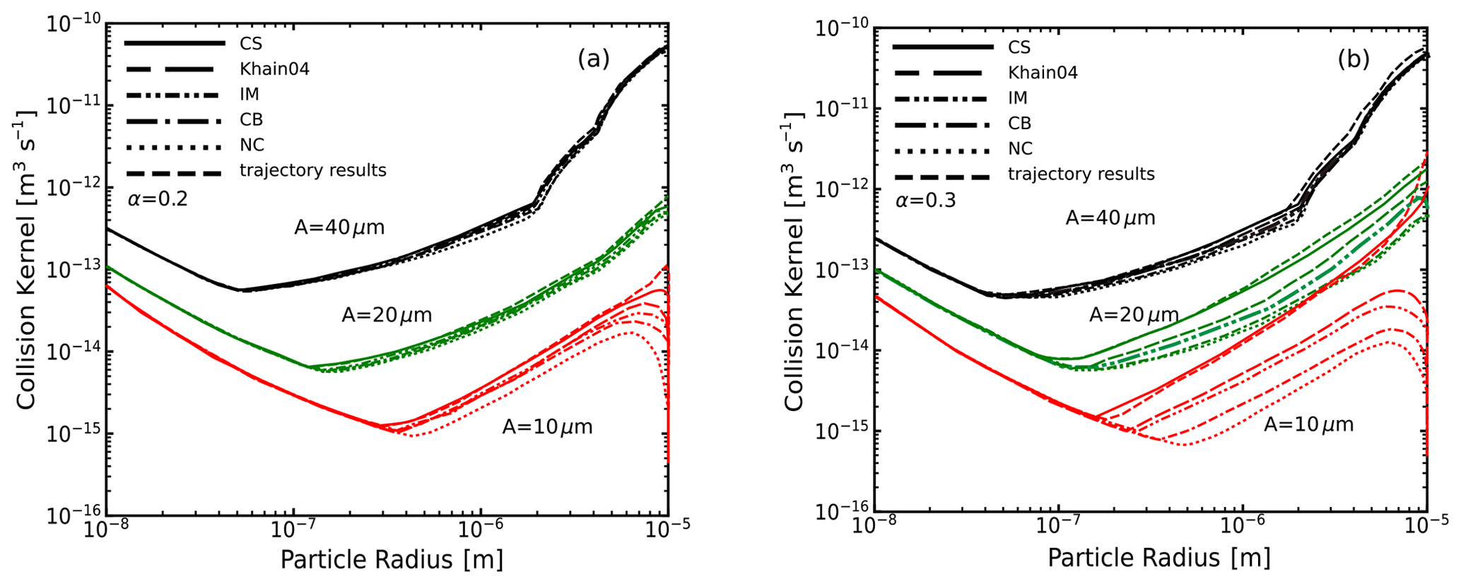
Figure 1Comparison of the effect of electric charge on the collision kernel for droplets of 40, 20, and 10 µm in size with small-droplet radii between 10−2 and 10 µm. The charging rate α is 0.2 for panel (a) and 0.3 for panel (b). The solid line represents the results where the collision kernel is calculated by the analytical expression and treats the charged droplets in a CS setting. The long-dashed line represents the results calculated by the analytical expression and treats the charge droplets in a Khain04 setting. The dashed–dotted–dotted line represents the results calculated by the analytical expression and treats the electrostatic electric force in an IM setting. The dashed–dotted line represents the results calculated by the analytical expression and treats the electrostatic electric force in a CB setting. The dotted line shows the results in an NC setting. The dashed line represents the results of the trajectory simulation according to Zhou et al. (2009).
Figure 1 displays a comparison of the collision–coalescence kernel for droplet radii of 40 µm (black lines), 20 µm (green lines), and 10 µm (red lines) across different calculation methods. The plots vary by line style to represent different analytical treatments and the inclusion or absence of static electric forces, with specific settings for the droplet-charging rate shown in Fig. 1a and b. The results indicate that the primary range for electro-coalescence is approximately 0.1 to 10 µm, which encompasses the Greenfield gap. When the small-droplet radius is less than 0.1 µm, the collision process is controlled by Brownian motion due to an excessively small number of charges on the small droplet. Conversely, when the radius of the droplets exceeds 10 µm, the collision process is primarily governed by gravity collision. The electric force has a larger effect on the smaller droplet. The electric force treated with the CS method has a larger effect on the collision–coalescence kernel than that with the IM method and the CB method. In the range of the Greenfield gap, the collision–coalescence kernels from the analytical method fit well with those from the trajectory method result. Note that the CB, Khain04, and IM methods do not take into account the collision of same-sized droplets; for the CS method, the Q2 term providing attractive or repulsive force between same-sized droplets ensures collision. For the range of droplets smaller than 10 µm, when the particle radius is close to 10 µm, the CB, Khain04, and IM methods deviate from the trajectory result, but the result of the CS method becomes over 2 times less than that of the trajectory method, where the collision process is controlled by the interception effect. The interception effect in particle collision–coalescence refers to the process where smaller particles are captured by a larger droplet's boundary layer and swept into it, even without direct contact, due to the aerodynamic air flow around the falling droplet. Although the analytical method cannot reproduce the interception effect, it can give the lower limit of estimation to the effect of the electric force effect with the conducting sphere method.
2.5 Numerical setup and schemes
Shima et al. (2009, 2020) constructed a particle-based cloud model, SCALE-SDM, by implementing the SDM into SCALE, which is a library of weather and climate models of the Earth and other planets (Nishizawa et al., 2015; Sato et al., 2015). Because of its efficient Monte Carlo algorithm for coalescence, the SDM particle-based scheme requires less computational cost to accurately simulate clouds and precipitation compared to the bin scheme (Shima et al., 2009). This study concentrates on warm-rain microphysics. We developed a numerical simulation using the latest version of SCALE-SDM, specifically employing the SDM warm-rain algorithm from Shima et al. (2009) rather than the SDM mixed-phase extension presented by Shima et al. (2020). We implemented the electro-coalescence process into the SDM's coalescence scheme as defined by Eqs. (5)–(18). The moist-air fluid dynamics in this study are computed using Eqs. (71)–(81) of Shima et al. (2020). The calculations utilise SCALE's dynamical core, which is based on a fully compressible non-hydrostatic equation. This approach is implemented on a staggered Arakawa C-grid (Arakawa and Lamb, 1977) using a finite-volume method.
For the initialisation of the super-particle, the “uniform sampling method” is applied as in previous works (Arabas and Shima, 2013; Shima et al., 2014, 2020; Sato et al., 2017, 2018). Unterstrasser et al. (2017) found that the uniform sampling method is more efficient than the “constant multiplicity method”. Then, the multiplicity of the super-droplets becomes proportional to the initial distribution function of real particles:
In SCALE-SDM, moist-air dynamics and cloud microphysics processes are integrated separately by using the first-order operator splitting scheme. Δt is set as the common time step. We set , and Δtcoal as the time steps for the advection and sedimentation of particles, condensation/evaporation, and collision–coalescence. We set Δtdyn as the time step for the fluid dynamics of moist air, which has to fulfil the Courant–Friedrichs–Lewy (CFL) condition of acoustic waves. All these time steps are divisors of the common time step Δt. The order of calculation in the model is as follows: (1) calculate the fluid dynamics without the coupling terms from the particles to moist air and update the moist air, (2) update the super-droplets from t to t+Δt, and (3) integrate one cloud microphysics process one time step forward and then move on to the next process. Processes lagging in time are calculated preferentially (for details, refer to Table 1 of Shima et al., 2020). Simultaneously, the feedback from particles to moist air comes through the coupling terms in Eqs. (75)–(79) of Shima et al. (2020), and we update the moist air from Glmn(t) to Glmn(t+Δt).
In our simulation, the domain of the simulation is two-dimensional (2D; x-z), 10 km in the horizontal and vertical directions with 50 m grid spacing, and the calculation time steps are Δt=0.4 s, Δtdyn=0.05 s, Δtadv=0.4 s, s, and Δtcoal=0.2 s. The initial super-droplet number concentration per grid cell is 128. We employ a subgrid-scale (SGS) turbulence model for dynamic processes but exclude it for cloud microphysics processes, such as collision–coalescence enhancement, velocity fluctuations, and supersaturation fluctuations. This approach might lead to an underestimation of the collision rate of charged droplets, as noted by Lu and Shaw (2015). Our simulations use a two-dimensional large-eddy simulation (LES) methodology. To assess the impact of fluctuations, we conduct a 50-member ensemble of simulations, varying the pseudo-random number sequence for each run.
2.6 Design of our numerical experiment
To evaluate the effect of electro-coalescence on warm clouds, 2D simulation of an isolated cumulus is performed following the setup of Lasher-Trapp et al. (2005). Note the original study of Lasher-Trapp et al. (2005) was conducted in 3D, but 2D simulation is used in this study to save computational resources. The initial profile of the atmosphere is horizontally uniform. The vertical profile of the moist air is given by sounding data from 15:45 UTC on 22 July from the Small Cumulus Microphysics Study (SCMS) in Florida. The cloud base is steady at 1050 m, and the maximum cloud-top height is 5350 m. As suggested by Lasher-Trapp et al. (2005), wind shear is assumed to be absent, and random velocity perturbation is applied (maximum of 0.5 m s−1) in the lowest kilometre of the model.
In general, there are different types of soluble/insoluble aerosols in a droplet. In the model, only one soluble substance ((NH4)HSO4 aerosol) is applied for simplicity. Initially, the aerosols are uniformly distributed in the simulation domain. The aerosol number concentration and size distribution were based on the data provided by vanZanten et al. (2011) for the RICO intercomparison case. The aerosol number concentration and size distribution are given by a bimodal log-normal distribution: the particle number concentrations of the two modes are N1=90 cm−3 and N2=15 cm−3, respectively. Note that aerosol concentrations are multiplied by factors of 3, 6, or 9, depending on the aerosol background conditions. The geometric mean radii are r1=0.03 µm and r2=0.14 µm, with geometric standard deviations of σ1=1.28 and σ2=1.75, respectively.
3.1 The effect of charged droplets on cloud evolution
Figure 2 presents snapshots of cloud structures at 1500, 2100, and 2700 s from a single simulation, illustrating the temporal changes in the mixing ratios of cloud water and rainwater. The results show that, with electro-coalescence in the CS setting (Fig. 2d–i), the cumulus takes a shorter time to form rain droplets than in the CB and no-charge (NC) settings. Comparing Fig. 2d–f and g–i shows that the electric force with the CS setting has a much stronger impact on the cloud evolution than with the CB setting. For the CS setting, there is heavy precipitation at 2700 s, while there is only haze for the CB and NC settings.
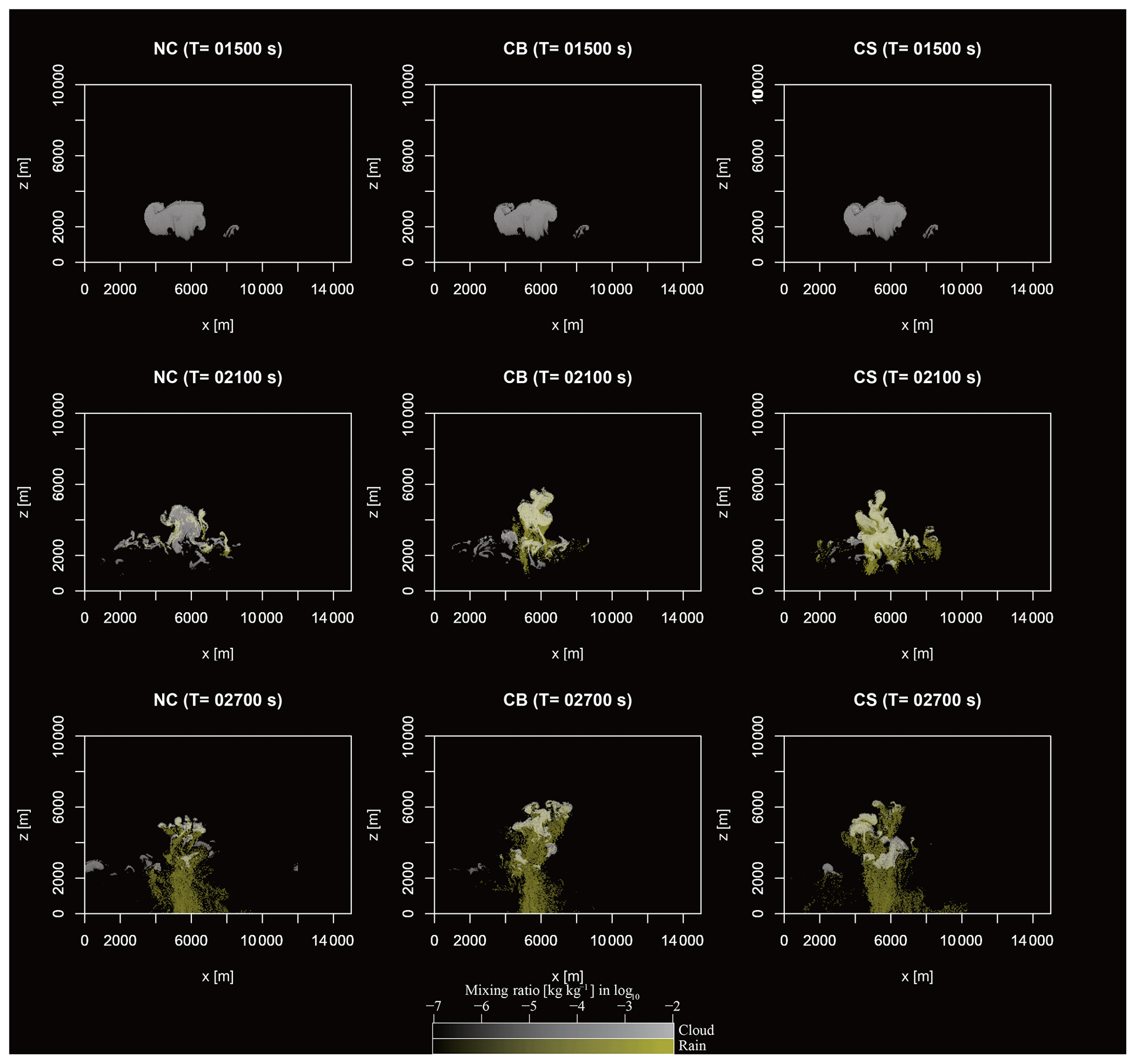
Figure 2A comparison of the spatial structure of the mixing ratio of hydrometeors of the cumulus with the NC setting, the electric force evaluated by the CB setting, and the electrostatic electric force evaluated by the CS setting at times of 1500, 2100, and 2700 s. The charging rate α is 0.3.
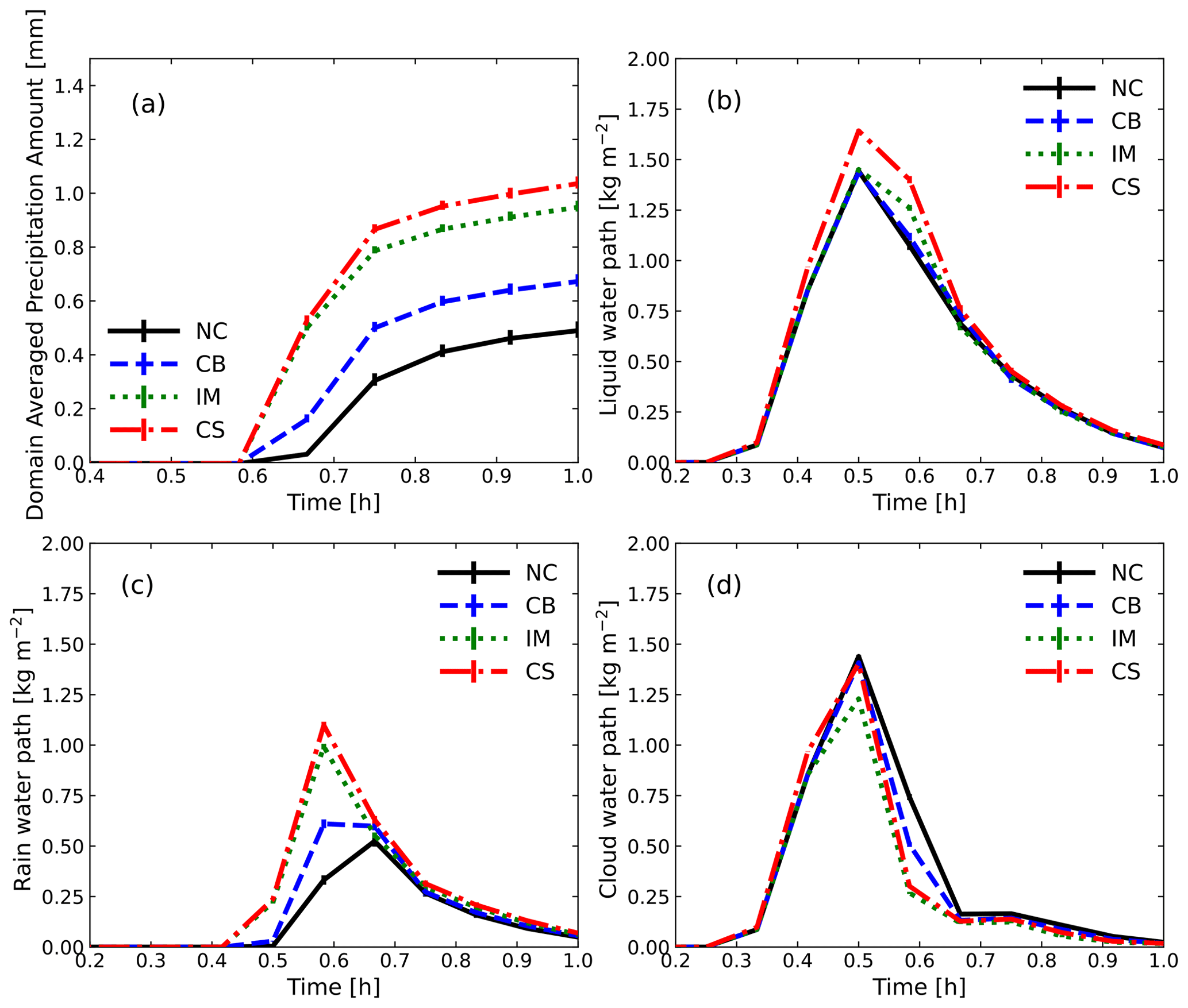
Figure 3The time evolution of the domain-averaged precipitation amount (a) and the domain-averaged water path of the liquid water path (b), rainwater path (c), and cloud water path (d), which is consistent with Fig. 2. The solid black line represents the NC setting, the dashed blue line represents the CB setting, the dotted green line represents the IM setting, and the dashed–dotted red line represents the CS setting. The error bar indicates the standard deviation calculated from 50 members of the random ensemble.
Figure 3a shows the time evolution of the domain and the average accumulated precipitation amount calculated from the 50-member random ensemble. Figure 3b–d shows the domain-averaged path, including the total liquid water path (Fig. 3b), rainwater path (Fig. 3c), and cloud water path (Fig. 3d). The error bar indicates the standard error, which is also calculated from the 50 members of the ensemble. An unbiased estimator is used to calculate the standard deviation error. The results show that the accumulated precipitation amount in the CS setting is 52.5 % higher than that in NC setting, 34.9 % higher than in the CB setting, and 8.4 % higher than in the IM setting. There is significant difference between the accumulated precipitation amounts in the NC setting, CS setting, IM setting, and CB setting. The initial precipitation time for all four settings starts at 2100 s. However, the total liquid water path and cloud path of the CB and NC settings are significantly higher than those of the CS setting because higher precipitation eliminates cloud evolution.
Figure 4 presents the droplet mass-density distributions during three stages of cloud development for the NC, CB, IM, and CS settings. At these three stages, the droplet size distribution in the CS setting is much wider and rain droplets are much coarser than in the NC, IM, and CB settings. At 21:00 s, there are two mass-density peaks of 10 and 1000 µm droplets for the NC, IM, CS, and CB settings, while the CS setting shows the highest mass density at 1000 µm, which is consistent with the results of Fig. 3.
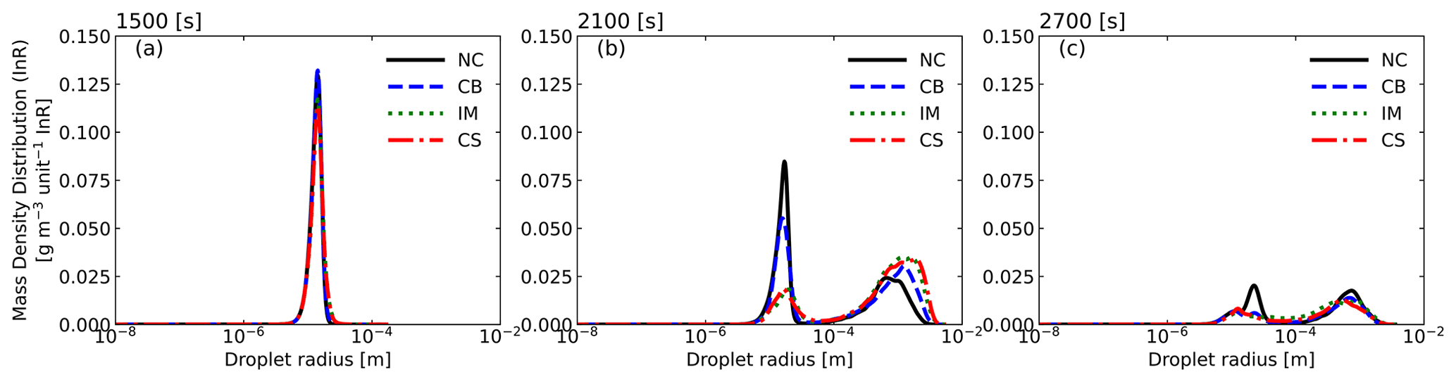
Figure 4The mass-density distribution evolution of the droplets at 1500 s (a), 2100 s (b), and 2700 s (c), which is consistent with Figs. 2 and 3. The solid black line represents the NC setting, the dashed blue line represents the CB setting, the dotted green line represents the IM setting, and the dashed–dotted red line represents the CS setting.
3.2 The effect of charge on droplets
Figure 5 shows the results of droplet time evolution (a)–(c) and the water fraction path (d)–(f) for charging rates (α) of 0.1, 0.2, and 0.6; the black line represents the NC setting. The results show that there are no significant differences between the results of the NC and CS settings with the charging rate α=0.1, which gives 0.3 % of the maximum charge on the droplets. With the enhancement of the charge on the droplets, clouds can form more rapidly. When the charging rate α=0.6, at 1500 s, there are larger droplets with radii over 1000 µm and even droplets of 5000 µm. However, cloud elimination is faster in conditions of higher charging rates: at 2700 s, conditions of lower charging rates result in a higher droplet mass density at a peak of approximately 1000 µm, which indicates that a higher charging rate results in a shorter lifetime of the cumulus cloud. The results of the domain water path, averaged over 50 ensembles in Fig. 5d–f, are consistent with those in Fig. 5a–c.
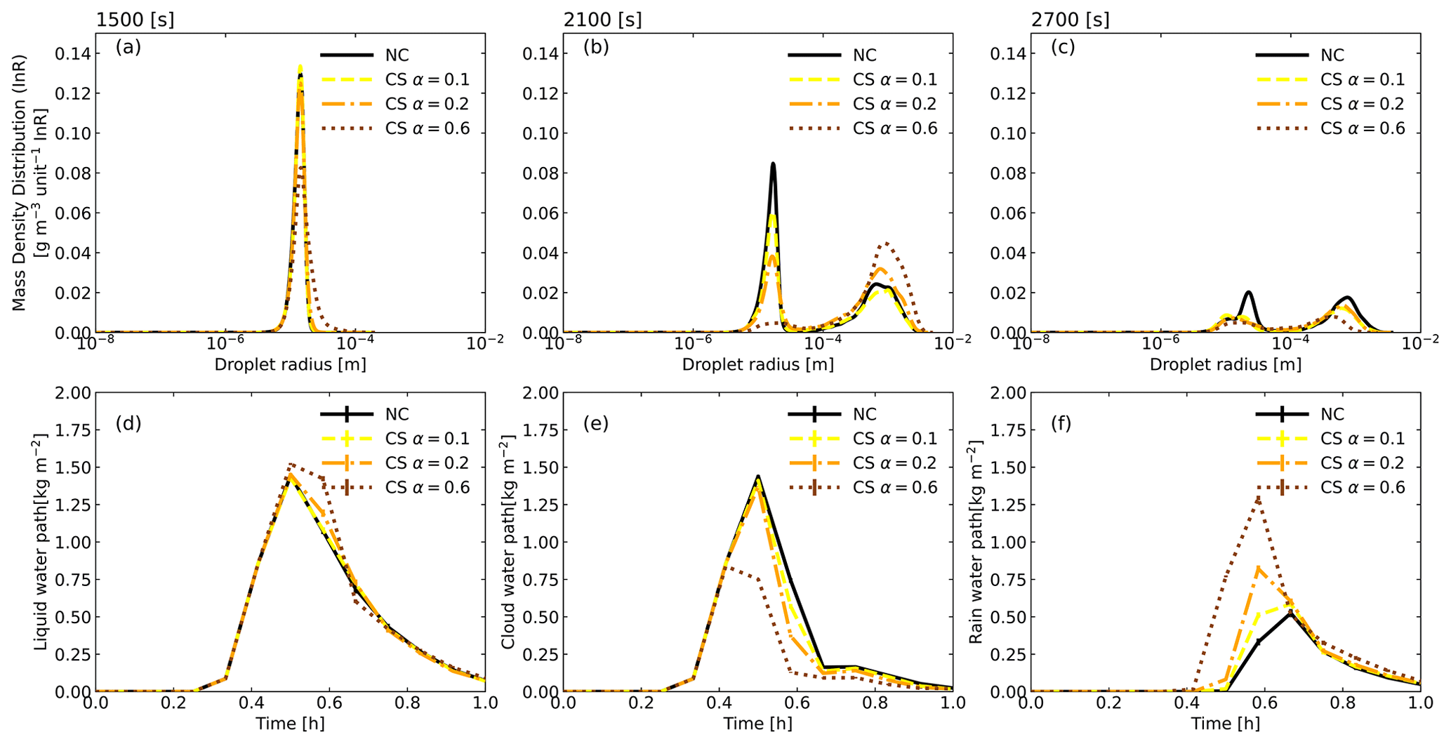
Figure 5Comparison of the cloud evolution for variable charging rates. The mass-density distribution of droplets at 1500 s (a), 2100 s (b), and 2700 s (c) and the time evolution of the domain-averaged water path of the liquid water path (LWP) (d), cloud water path (CWP) (e), and rainwater path (RWP) (f) are presented for charging rates (α) of 0.1 (solid yellow line), 0.2 (dashed–dotted orange line), and 0.6 (dotted brown line).
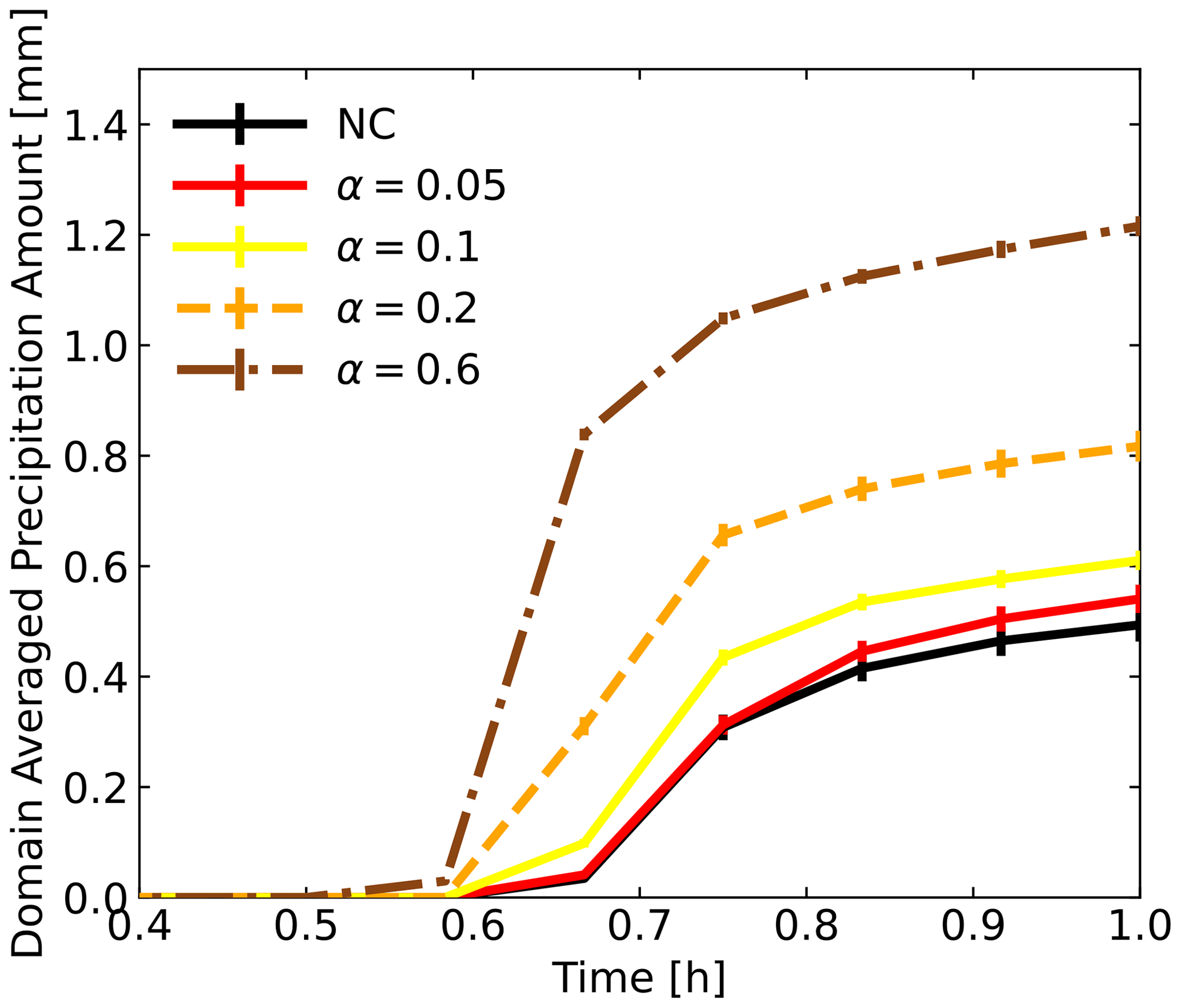
Figure 6A comparison of the evolution of the domain-averaged precipitation amount with variable droplet-charging rates (α) of 0.05 (solid red line), 0.1 (solid yellow line), 0.2 (dashed orange line), and 0.6 (dashed–dotted brown line), and the electric force is evaluated with the CS setting. The solid black line represents the NC setting.
Figure 6 shows the domain- and ensemble-averaged precipitation amount as a function of the droplet-charging rate in the CS setting. Similarly to the results in Fig. 5, clouds with higher-charging-rate conditions produce precipitation earlier than those under low-charging-rate conditions. With the enhancement of the charging rate, the precipitation amount at 3500 s does not simultaneously increase under all conditions. When the charging rate is 0.6, the final precipitation amount decreases due to more liquid water and cloud water loss in the early stage of cloud formation. In Fig. 6, the result of the CS-setting charging rate α=0.05, which is 0.16 % of the maximum charge on the droplets, is given by the solid orange line, and the precipitation amount is 9.5 % higher than that of the NC setting.
3.3 The effect of the aerosol concentration
Figure 7 illustrates the average precipitation amounts for 50 ensemble simulations under the CS setting, plotted as a function of aerosol concentrations. The results are shown for low (solid line), medium (dotted line), and high (dashed–dotted line) aerosol concentrations, with a charging rate of 0.2. The blue, pink, and purple lines represent the results of low-aerosol (LA), medium-aerosol (MA), and high-aerosol (HA) conditions with the NC setting. Under NC settings, the Twomey effect demonstrates that higher aerosol concentrations lead to smaller particle radii in clouds, reducing precipitation efficiency. Conversely, when electrostatic forces are introduced, these higher aerosol concentrations substantially enhance precipitation across different scenarios. Specifically, in HA conditions, the precipitation enhancement reaches 782 % over the NC setting; for MA conditions, it is 467 % higher; and, for LA conditions, the increase is 110 %. This illustrates the significant role electrostatic forces play in modulating cloud dynamics and precipitation responses to aerosol variations.
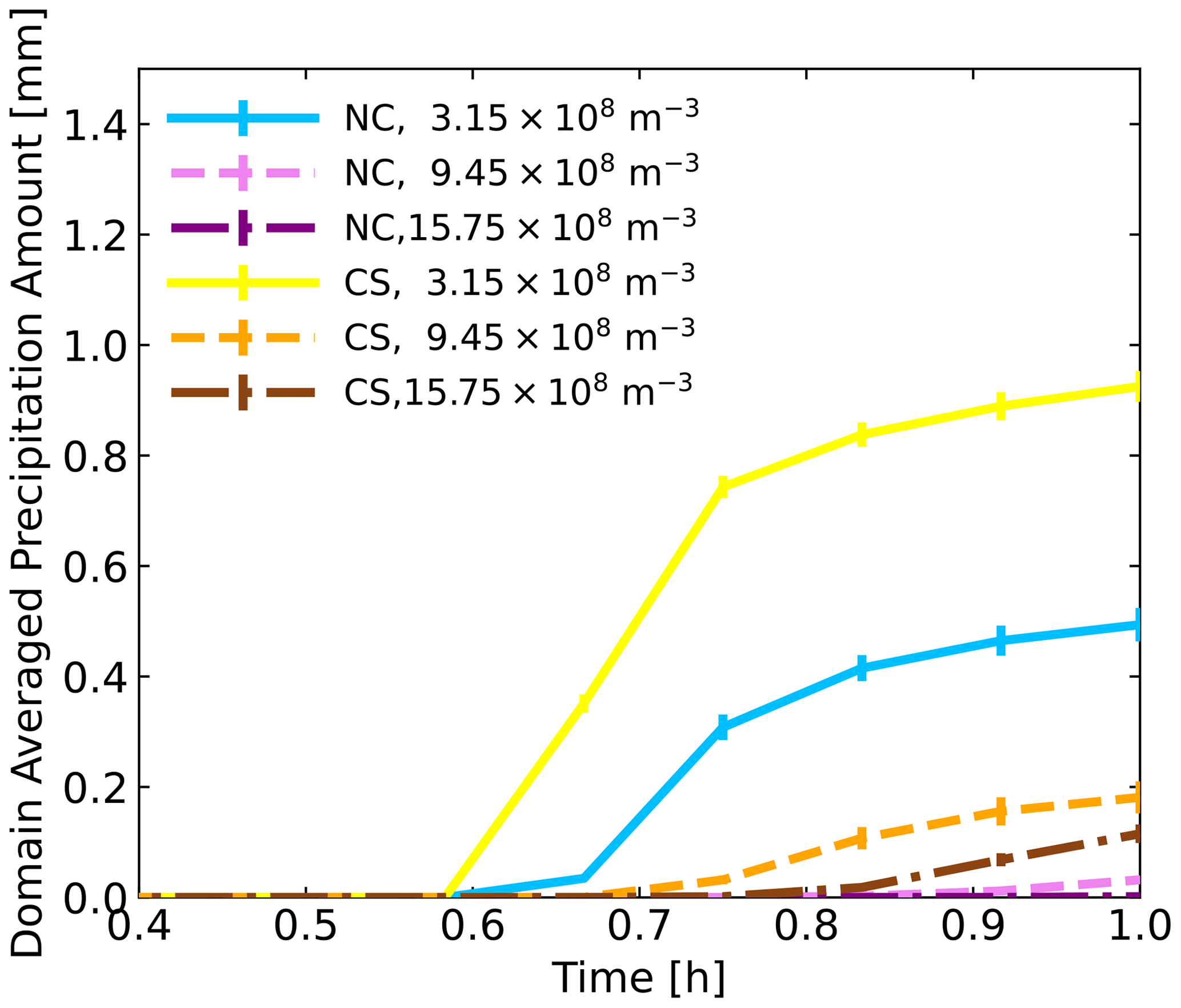
Figure 7The time evolution of the domain-averaged precipitation of the aerosol concentration represented by solid lines (LA, 3.15×10⁸ m−3), dotted lines (MA, 9.45×10⁸ m−3), and dashed–dotted lines (HA, 15.75×10⁸ m−3). The yellow, orange, and brown lines represent the simulation with the electric force in LA, MA, and HA conditions, respectively, which is evaluated with the CS setting, where the charging rate α is 0.2. Blue, pink, and purple lines represent the simulation with the NC setting in LA, MA, and HA conditions, respectively.
3.4 Comparison of different electrostatic force calculations
Figure 8 presents the domain-averaged precipitation amounts under different electrostatic force settings with a charging rate of 0.3, illustrated by various line styles for each setting. The dashed blue line represents the result of droplets with opposite-sign charges and the setting based on the Khain04 method. The upper limit of the charge on the small droplets is 50 elementary charges, the lower limit of the charge on the droplets is 1 elementary charge, and the pink dashed–dotted line represents the special setting of only a large droplet charged with electrostatic force by the CS method (CS-q0). For the CS, Khain04, and IM settings, precipitation increases at 2100 s, which is 300 s before the NC setting. The domain- and ensemble-averaged precipitation amount with the CS setting is 52.5 % higher than with the NC setting; with the Khain04 setting, it is 5.42 % larger; with the CS-q0 setting, it is 9.6 % larger; and with the IM setting, it is 8.45 % larger.
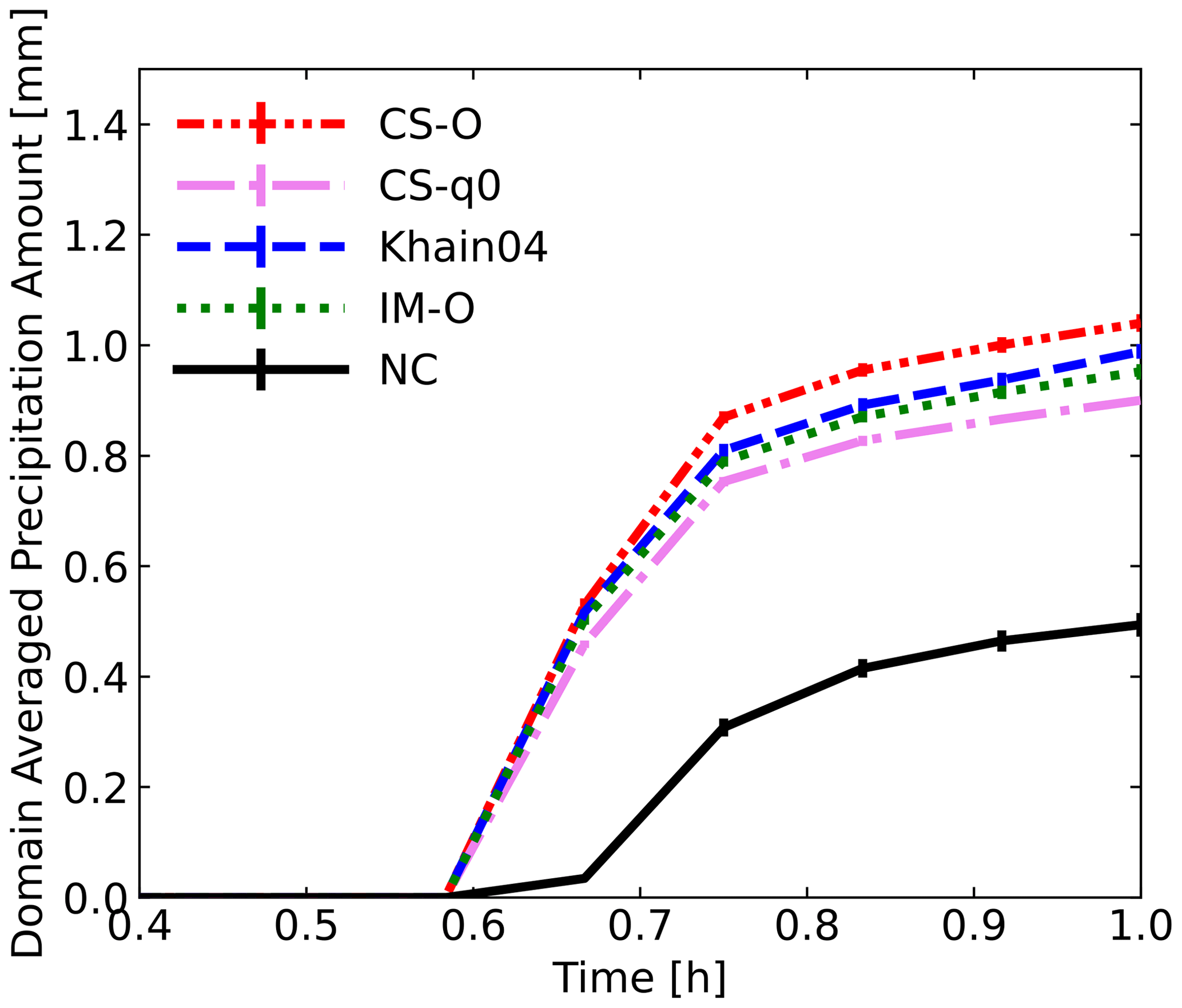
Figure 8Comparison of the time evolution of the domain-averaged precipitation amount for variable evaluation of the electric force. The solid black line represents the NC setting. The dashed–dotted lines represent the results of the electric force evaluated by the CS method. The dashed–dotted red line represents the result of droplets with opposite-sign charges. The dashed-dotted pink line represents the condition where the charge is only on the large droplet, and the dashed blue line represents the result of droplets with opposite-sign charges and the CS method based on Khain et al. (2004). The dotted green line is the result of droplets with opposite-sign charges, and the electric force is evaluated by the image charge method.
When the two droplets move together and coalesce, there are three sites where collisions can occur: the front, side, and rear. The radius ratio between a large droplet and a small droplet (RARA) controls the collision site, and when the radius of the small droplet is less than 0.1 µm and the RARA is larger than 100, the collision is a rear collision. For front and side collisions, in clouds where the droplet size is less than 40 µm and the relative humidity is 100 %, the droplet collision is controlled by the balance of the Stokes drag of the air flow and electric force. The analytic expression in our work suggested by Davenport and Peters (1978) can give a good estimation, especially for the Greenfield gap part, although, in the front- and side-collision regions when the RARA is close to 1, the additional contribution due to the interception associated with the electric effect cannot be fully reproduced by this method. For the rear collision, the flow drag, electric force, and Brownian motion of the small droplet can impact the collision process. In the present work, because the charge on the droplet varies as a function of the droplet radius, there is less than 1 elementary charge on a droplet with a radius less than 0.1 µm. Therefore, the electric force does not have a significant effect on the collision process even for droplets of opposite signs, and the Brownian collision efficiency could be good enough for estimation under these conditions. When the amount of charge on a small droplet is over several elementary charges due to the evaporation of a large droplet with a large amount of charge, the rear collision could be significantly affected by the electric force (Tinsley and Leddon, 2013). The net attractive force of droplets with opposite signs increases the collision efficiency, and the net repulsive force of droplets with the same sign decreases the collision efficiency; this is called electro-anti-coalescence. As Tinsley et al. (2001) mentioned, below the cloud-bottom boundary, there could be a highly charged nucleus or small droplet with tens to hundreds of elementary charges due to the evaporation of a highly charged droplet. These highly charged small droplets or nuclei could be moved into the cloud by upward air flow, which is not considered in this paper.
In clouds, there are several ways to charge droplets, and, in the cloud boundary, due to charging by the vertical electric current density (Jz) from the ionosphere to the ground surface, a droplet in the cloud-top boundary accumulates a positive charge and a droplet in the cloud-bottom boundary accumulates a net negative charge; this has been shown by simulations (Zhou and Tinsley, 2007, 2012) and field observations (Nicoll and Harrison, 2016). With the charging rate of 0.05, there are on the order of 100 elementary charges on a droplet with a radius of 10 µm, which is consistent with observation (Beard et al., 2004) and simulation (Zhou and Tinsley, 2007) results. Therefore, in the stratus cloud, most droplet collisions occur between droplets of the same sign or between one charged droplet and one uncharged droplet. Using the CS method, the additional electrostatic force due to the multiple-image dipoles between the colliding droplets can be addressed, even if the droplets have the same sign charges or a small droplet is uncharged. Khain et al. (2004) evaluated the electro-coalescence effect on warm-cloud rain enhancement and fog formation based on the image charge method from one induced dipole on each droplet by the bin scheme. Zhou et al. (2009) claimed that, when the RARA is close to 1, the collision efficiency calculated by the CS method, which treats the multiple induced dipoles on each droplet, is twice as large as that calculated with the IM method. Therefore, for the Greenfield gap region and the interception region, the evaluation of the charge effect with the CS method is more accurate, and the SDM particle-based approach provides a superior performance to bin schemes (Li et al., 2017). In Fig. 8, due to the additional induced image charge on droplets, the maximum average precipitation amount of the CS setting is 8.45 % larger than that of the IM setting. Despite a 30 % increase in computation burden, the CS method for electrostatic force should be incorporated into the cloud microphysics scheme. The CS method provides superior numerical stability and accuracy in simulating charge droplet interactions, particularly for charge droplets of similar size. Khain et al. (2004) evaluated electro-coalescence at a low charging rate of 5 % of the maximum charge on droplets. In our simulation, we tested charging rates (α) ranging from 0.05 to 0.6, equivalent to 0.15 % to 1.8 % of the maximum charge. At a charging rate of 0.3, the electric force evaluated by the CS method increased domain- and ensemble-averaged precipitation by approximately 5.42 % compared to the Khain04 setting. The results indicate that, even with weak charging, the electro-coalescence effect significantly increases precipitation.
Tinsley et al. (2001), Tinsley and Zhou (2006) and Zhou et al. (2009) claimed that the induced charge on droplets of the same sign could produce a short-range attractive electrostatic force that increases the collision efficiencies. The charge on the large droplets could exert an additional short-range attraction on the small droplet, even if there is no charge or the same charge on the small droplets. However, for droplets of the same sign, the short-range electrostatic force has a significant effect only if the charge ratio between the large droplet and small droplet, Q:q, is greater than 100 or q:Q is greater than 1. For Q:q ratios larger than 100, the additional image charge effect on the small droplet due to the large charged droplet controls the collision process. For q:Q greater than 1, the additional image charge effect is due to the small charged droplet.
The SDM particle-based approach explicitly provides cloud–aerosol interaction simulations, such as the role of CCN in rain formation (Grabowski et al., 2019). According to our simulation results, the electro-coalescence effect on precipitation is sensitive to the aerosol concentration. With a high aerosol concentration, the average precipitation with an electric effect could be a factor of 4 higher than in NC conditions. A much higher aerosol concentration corresponds to a more sensitive cloud response to the electrostatic force. Then, under high-aerosol-concentration conditions, a small variation in Jz could have a significant effect on cloud formation. Alternatively, in highly polluted clouds, placing a small number of charged aerosols or droplets accelerates rain enhancement due to electro-coalescence.
The electro-coalescence effect on a weakly electrified warm cumulus cloud was revisited. Assuming droplets with opposite signs are charged instantaneously by Jz, the amount of charge is determined by the size of the droplets. A new simulation with the exact treatment of the electrostatic force for an opposite-sign charge case based on the SDM particle-based approach provides a good estimation of the effect of electro-coalescence in the Greenfield gap region. In the simulation, droplets smaller than 0.1 µm are controlled by Brownian motion. The results show that, for droplets of opposite signs with the same treatment of the electrostatic force, the cloud evolution can be significantly changed as a function of the arbitrarily prescribed charging rate α. The case of droplets with same-sign charge (Tinsley and Zhou, 2015) and the charge amount prediction are necessary for accurate simulation. Electro-coalescence has a larger impact on highly polluted warm cumulus clouds.
Cloud radiation feedback is one of the sources of uncertainty in the climate model (Zelinka et al., 2017). The electrostatic force effect parameterisation for different cloud types should be indicated to improve climate model accuracy. This study reveals the electrostatic force effect on warm cumulus clouds, contributing to the parameterisation of electrostatic microphysical processes.
The SCALE library was developed by Team-SCALE of the RIKEN Center for Computational Sciences (https://scale.riken.jp/, last access: 2 September 2024); note that the SDM code is not accessible through this site. The source code of SCALE-SDM 0.2.5–2.3.0 and the single-simulation data of α=0.3 in four settings of NC, CB, IM, and CS are available on Zenodo (Zhang, 2024, https://doi.org/10.5281/zenodo.11058066). All data used for this study can be reproduced by following the instructions included in the above repository. The data are also deposited in local storage at the University of Hyogo, Japan.
All the authors designed the model and numerical experiments. LM and SS developed the model code, and RZ performed the simulations. RZ prepared the article with contributions from all co-authors.
The contact author has declared that none of the authors has any competing interests.
Publisher’s note: Copernicus Publications remains neutral with regard to jurisdictional claims made in the text, published maps, institutional affiliations, or any other geographical representation in this paper. While Copernicus Publications makes every effort to include appropriate place names, the final responsibility lies with the authors.
The authors sincerely appreciate the insightful and constructive comments provided by the topical editor, Nina Crnivec, reviewer Emily de Jong, and an anonymous referee.
This work was funded in part by the Strategic Priority Research Program of CAS (grant no. XDB 41000000), the National Natural Science Foundation of China (grant nos. 42271027 and 41971020), MEXT KAKENHI (grant no. 18H04448), JSPS KAKENHI (grant nos. 26286089, 20H00225, and 23H00149), JST's Moonshot R and D (grant no. JPMJMS2286), and the China Scholarship Council (grant no. 202106140113).
This paper was edited by Nina Crnivec and reviewed by Emily de Jong and one anonymous referee.
Andronache, C.: Diffusion and electric charge contributions to below-cloud wet removal of atmospheric ultra-fine aerosol particles, J. Aerosol Sci., 35, 1467–1482, https://doi.org/10.1016/j.jaerosci.2004.07.005, 2004.
Arabas, S. and Shima, S.-i.: Large-eddy simulations of trade wind cumuli using particle-based microphysics with monte carlo coalescence, J. Atmos. Sci., 70, 2768–2777, https://doi.org/10.1175/JAS-D-12-0295.1, 2013.
Arakawa, A. and Lamb, V. R.: Computational design of the basic dynamical processes of the UCLA general circulation model, Meth. Comput. Phys., 17, 173–265, https://doi.org/10.1016/B978-0-12-460817-7.50009-4, 1977.
Ardon-Dryer, K., Huang, Y.-W., and Cziczo, D. J.: Laboratory studies of collection efficiency of sub-micrometer aerosol particles by cloud droplets on a single-droplet basis, Atmos. Chem. Phys., 15, 9159–9171, https://doi.org/10.5194/acp-15-9159-2015, 2015.
Beard, K. V., Ochs III, H. T., and Twohy, C. H.: Aircraft measurements of high average charges on cloud drops in layer clouds, Geophys. Res. Lett., 31, L14111, https://doi.org/10.1029/2004GL020465, 2004.
Bleaney, B. I. and Bleaney, B.: Electricity and Magnetism, Volume 1, Oxford University Press, 676 pp., ISBN 9780199645428, 1993.
Bott, A.: A flux method for the numerical solution of the stochastic collection equation, J. Atmos. Sci., 55, 2284–2293, https://doi.org/10.1175/1520-0469(1998)055<2284:afmftn>2.0.co;2, 1998.
Davenport, H. M. and Peters, L. K.: Field studies of atmospheric particulate concentration changes during precipitation, Atmos. Environ., 12, 997–1008, https://doi.org/10.1016/0004-6981(78)90344-X, 1978.
Davis, M. H.: Two charged spherical conductors in a uniform electric field: Forces and field strength, Q. J. Mech. Appl. Math., 17, 499–511, https://doi.org/10.1093/qjmam/17.4.499, 1964.
Davis, M. H.: Collisions of small cloud droplets: gas kinetic effects, J. Atmos. Sci., 29, 911–915, https://doi.org/10.1175/1520-0469(1972)029<0911:COSCDG>2.0.CO;2, 1972.
Frederick, J. E. and Tinsley, B. A.: The response of longwave radiation at the South Pole to electrical and magnetic variations: Links to meteorological generators and the solar wind, J. Atmos. Sol.-Terr. Phys., 179, 214–224, https://doi.org/10.1016/j.jastp.2018.08.003, 2018.
Frederick, J. E., Tinsley, B. A., and Zhou, L.: Relationships between the solar wind magnetic field and ground-level longwave irradiance at high northern latitudes, J. Atmos. Sol.-Terr. Phys., 193, 105063, https://doi.org/10.1016/j.jastp.2019.105063, 2019.
Grabowski, W. W. and Wang, L.-P.: Growth of Cloud Droplets in a Turbulent Environment, Annu. Rev. Fluid Mech., 45, 293–324, https://doi.org/10.1146/annurev-fluid-011212-140750, 2013.
Grabowski, W. W., Morrison, H., Shima, S.-I., Abade, G. C., Dziekan, P., and Pawlowska, H.: Modeling of Cloud Microphysics: Can We Do Better?, B. Am. Meteorol. Soc., 100, 655–672, https://doi.org/10.1175/BAMS-D-18-0005.1, 2019.
Greenfield, S. M.: Rain scavenging of radioactive particulate matter from the atmosphere, J. Atmos. Sci., 14, 115–125, https://doi.org/10.1175/1520-0469(1957)014<0115:RSORPM>2.0.CO;2, 1957.
Guo, S. and Xue, H.: The enhancement of droplet collision by electric charges and atmospheric electric fields, Atmos. Chem. Phys., 21, 69–85, https://doi.org/10.5194/acp-21-69-2021, 2021.
Hall, W. D.: A detailed microphysical model within a two-dimensional dynamic framework: model description and preliminary results, J. Atmos. Sci., 37, 2486–2507, https://doi.org/10.1175/1520-0469(1980)037<2486:ADMMWA>2.0.CO;2, 1980.
Jonas, P. R.: The collision efficiency of small drops, Quarterly J. Roy. Meteor. Soc., 98, 681–683, https://doi.org/10.1002/qj.49709841717, 1972.
Khain, A., Arkhipov, V., Pinsky, M., Feldman, Y., and Ryabov, Y.: Rain enhancement and fog elimination by seeding with charged droplets. part I: theory and numerical simulations, J. Appl. Meteorol., 43, 1513–1529, https://doi.org/10.1175/JAM2131.1, 2004.
Kniveton, D. R., Tinsley, B. A., Burns, G. B., Bering, E. A., and Troshichev, O. A.: Variations in global cloud cover and the fair-weather vertical electric field, J. Atmos. Sol.-Terr. Phys., 70, 1633–1642, https://doi.org/10.1016/j.jastp.2008.07.001, 2008.
Köhler, H.: The nucleus in and the growth of hygroscopic droplets, T. Faraday Soc., 32, 1152–1161, https://doi.org/10.1039/TF9363201152, 1936.
Fuchs, N. A.: The Mechanics of Aerosols, Revised and Enlarged, Pergamon Press Oxford, Oxford, https://doi.org/10.1002/qj.49709138822, 1964.
Lam, M. M., Chisham, G., and Freeman, M. P.: Solar wind-driven geopotential height anomalies originate in the Antarctic lower troposphere, Geophys. Res. Lett., 41, 6509–6514, https://doi.org/10.1002/2014GL061421, 2014.
Lasher-Trapp, S. G., Cooper, W. A., and Blyth, A. M.: Broadening of droplet size distributions from entrainment and mixing in a cumulus cloud, Q. J. Roy. Meteor. Soc., 131, 195–220, https://doi.org/10.1256/qj.03.199, 2005.
Li, X.-Y., Brandenburg, A., Haugen, N. E. L., and Svensson, G.: Eulerian and Lagrangian approaches to multidimensional condensation and collection, J. Adv. Model. Earth Sy., 9, 1116–1137, https://doi.org/10.1002/2017MS000930, 2017.
Liu, Y., Yau, M.-K., Shima, S.-i., Lu, C., and Chen, S.: Parameterization and Explicit Modeling of Cloud Microphysics: Approaches, Challenges, and Future Directions, Adv. Atmos. Sci., 40, 747–790, https://doi.org/10.1007/s00376-022-2077-3, 2023.
Lu, J. and Shaw, R. A.: Charged particle dynamics in turbulence: Theory and direct numerical simulations, Phys. Fluids, 27,, 065111, https://doi.org/10.1063/1.4922645, 2015.
Meek, J. M. and Craggs, J. D.: Electrical breakdown of gases, Q. J. Roy. Meteor. Soc., 80, 282–283, https://doi.org/10.1002/qj.49708034425, 1954.
Montero-Martínez, G., Kostinski, A. B., Shaw, R. A., and García-García, F.: Do all raindrops fall at terminal speed?, Geophys. Res. Lett., 36, L11818, https://doi.org/10.1029/2008GL037111, 2009.
Nicoll, K. A. and Harrison, R. G.: Stratiform cloud electrification: comparison of theory with multiple in-cloud measurements, Q. J. Roy. Meteor. Soc., 142, 2679–2691, https://doi.org/10.1002/qj.2858, 2016.
Nishizawa, S., Yashiro, H., Sato, Y., Miyamoto, Y., and Tomita, H.: Influence of grid aspect ratio on planetary boundary layer turbulence in large-eddy simulations, Geosci. Model Dev., 8, 3393–3419, https://doi.org/10.5194/gmd-8-3393-2015, 2015.
Pruppacher, H. R. and Klett, J. D.: Microphysics of clouds and precipitation, Springer Dordrecht, https://doi.org/10.1007/978-0-306-48100-0, 2010.
Rayleigh, L.: The influence of electricity on colliding water drops, P. Roy. Soc. Lond., 28, 405–409, 1878.
Rogers, R. R. and Yau, M. K.: A Short Course in Cloud Physics, Elsevier Science, ISBN 9780750632157, 1989.
Sato, Y., Nishizawa, S., Yashiro, H., Miyamoto, Y., Kajikawa, Y., and Tomita, H.: Impacts of cloud microphysics on trade wind cumulus: which cloud microphysics processes contribute to the diversity in a large eddy simulation?, Prog. Earth Planet. Sci., 2, 23, https://doi.org/10.1186/s40645-015-0053-6, 2015.
Sato, Y., Shima, S.-i., and Tomita, H.: A grid refinement study of trade wind cumuli simulated by a Lagrangian cloud microphysical model: the super-droplet method, Atmos. Sci. Lett., 18, 359–365, https://doi.org/10.1002/asl.764, 2017.
Sato, Y., Shima, S.-i., and Tomita, H.: Numerical convergence of shallow convection cloud field simulations: comparison between double-moment Eulerian and particle-based Lagrangian microphysics coupled to the same dynamical core, J. Adv. Model. Earth Sy., 10, 1495–1512, https://doi.org/10.1029/2018MS001285, 2018.
Seeßelberg, M., Trautmann, T., and Thorn, M.: Stochastic simulations as a benchmark for mathematical methods solving the coalescence equation, Atmos. Res., 40, 33–48, https://doi.org/10.1016/0169-8095(95)00024-0, 1996.
Seinfeld, J. H. and Pandis, S. N.: Atmospheric Chemistry and Physics: From Air Pollution to Climate Change, Wiley, ISBN 1118947401, 2006.
Shima, S., Kusano, K., Kawano, A., Sugiyama, T., and Kawahara, S.: The super-droplet method for the numerical simulation of clouds and precipitation: a particle-based and probabilistic microphysics model coupled with a non-hydrostatic model, Q. J. Roy. Meteor. Soc., 135, 1307–1320, https://doi.org/10.1002/qj.441, 2009.
Shima, S., Sato, Y., Hashimoto, A., and Misumi, R.: Predicting the morphology of ice particles in deep convection using the super-droplet method: development and evaluation of SCALE-SDM 0.2.5-2.2.0, -2.2.1, and -2.2.2, Geosci. Model Dev., 13, 4107–4157, https://doi.org/10.5194/gmd-13-4107-2020, 2020.
Shima, S.-i., Hasegawa, K., and Kusano, K.: Preliminary numerical study on the cumulus-stratus transition induced by the increase of formation rate of aerosols, Low Temperature Science, 72, 249–264, 2014 (in Japanese).
Tinsley, B. A.: The global atmospheric electric circuit and its effects on cloud microphysics, Rep. Progr. Phys., 71, 066801, https://doi.org/10.1088/0034-4885/71/6/066801, 2008.
Tinsley, B. A. and Leddon, D. B.: Charge modulation of scavenging in clouds: Extension of Monte Carlo simulations and initial parameterization, J. Geophys. Res.-Atmos., 118, 8612–8624, https://doi.org/10.1002/jgrd.50618, 2013.
Tinsley, B. A. and Zhou, L.: Initial results of a global circuit model with variable stratospheric and tropospheric aerosols, J. Geophys. Res., 111, D16205, https://doi.org/10.1029/2005jd006988, 2006.
Tinsley, B. A. and Zhou, L.: Parameterization of aerosol scavenging due to atmospheric ionization, J. Geophys. Res.-Atmos., 120, 8389–8410, https://doi.org/10.1002/2014jd023016, 2015.
Tinsley, B. A., Rohrbaugh, R. P., and Hei, M.: Electroscavenging in clouds with broad droplet size distributions and weak electrification, Atmos. Res., 59–60, 115–135, https://doi.org/10.1016/s0169-8095(01)00112-0, 2001.
Tripathi, S. N., Vishnoi, S., Kumar, S., and Harrison, R. G.: Computationally efficient expressions for the collision efficiency between electrically charged aerosol particles and cloud droplets, Q. J. Roy. Meteor. Soc., 132, 1717–1731, https://doi.org/10.1256/qj.05.125, 2006.
Tripathi, S. N., Michael, M., and Harrison, R. G.: Profiles of Ion and Aerosol Interactions in Planetary Atmospheres, Space Sci. Rev., 137, 193–211, https://doi.org/10.1007/s11214-008-9367-7, 2008.
Unterstrasser, S., Hoffmann, F., and Lerch, M.: Collection/aggregation algorithms in Lagrangian cloud microphysical models: rigorous evaluation in box model simulations, Geosci. Model Dev., 10, 1521–1548, https://doi.org/10.5194/gmd-10-1521-2017, 2017.
vanZanten, M. C., Stevens, B., Nuijens, L., Siebesma, A. P., Ackerman, A. S., Burnet, F., Cheng, A., Couvreux, F., Jiang, H., Khairoutdinov, M., Kogan, Y., Lewellen, D. C., Mechem, D., Nakamura, K., Noda, A., Shipway, B. J., Slawinska, J., Wang, S., and Wyszogrodzki, A.: Controls on precipitation and cloudiness in simulations of trade-wind cumulus as observed during RICO, J. Adv. Model. Earth Sy., 3, M06001, https://doi.org/10.1029/2011MS000056, 2011.
Wang, F., Zhang, Y., and Zheng, D.: Impact of updraft on neutralized charge rate by lightning in thunderstorms: A simulation case study, J. Meteorol. Res., 29, 997–1010, https://doi.org/10.1007/s13351-015-5023-9, 2015.
Wang, P. K., Grover, S. N., and Pruppacher, H. R.: On the effect of electric charges on the scavenging of aerosol particles by clouds and small raindrops, J. Atmos. Sci., 35, 1735–1743, https://doi.org/10.1175/1520-0469(1978)035<1735:OTEOEC>2.0.CO;2, 1978.
Weon, B. M. and Je, J. H.: Charge-induced wetting of aerosols, Appl. Phys. Lett., 96, 194101, https://doi.org/10.1063/1.3430007, 2010.
Zelinka, M. D., Randall, D. A., Webb, M. J., and Klein, S. A.: Clearing clouds of uncertainty, Nat. Clim. Change, 7, 674–678, https://doi.org/10.1038/nclimate3402, 2017.
Zhang, L., Tinsley, B. A., and Zhou, L.: Parameterization of in-cloud aerosol scavenging due to atmospheric ionization: Part 3. effects of varying droplet radius, J. Geophys. Res.-Atmos., 123, 10546–10567, https://doi.org/10.1029/2018jd028840, 2018.
Zhang, R.: Ruyizhang2333/SCALE-SDM-electro-coalescence: SCALE-SDM-electro-coalescence-v0.3 (v0.3), Zenodo [code], https://doi.org/10.5281/zenodo.11058066, 2024.
Zhou, L. and Tinsley, B. A.: Production of space charge at the boundaries of layer clouds, J. Geophys. Res.-Atmos., 112, D11203, https://doi.org/10.1029/2006jd007998, 2007.
Zhou, L. and Tinsley, B. A.: Time dependent charging of layer clouds in the global electric circuit, Adv. Space Res., 50, 828–842, https://doi.org/10.1016/j.asr.2011.12.018, 2012.
Zhou, L., Tinsley, B. A., and Plemmons, A.: Scavenging in weakly electrified saturated and subsaturated clouds, treating aerosol particles and droplets as conducting spheres, J. Geophys. Res., 114, D18201, https://doi.org/10.1029/2008jd011527, 2009.