the Creative Commons Attribution 4.0 License.
the Creative Commons Attribution 4.0 License.
 | 12 Sep 2024
The Measurement Error Proxy System Model: MEPSM v0.2
Proxy system models (PSMs) are an essential component of paleoclimate data assimilation and for testing climate field reconstruction methods. Generally, current statistical PSMs consider the noise in the output (proxy) variable only and ignore the noise in the input (environmental) variables. This problem is exacerbated when there are several input variables. Here we develop a new PSM, the Measurement Error Proxy System Model (MEPSM), which includes noise in all variables, including noise auto- and cross-correlation. The MEPSM is calibrated using a quasi-Bayesian solution, which leverages Gaussian conjugacy to produce a fast solution. Another advantage of MEPSM is that the prior can be used to stabilize the solution between an informative prior (e.g., with a non-zero mean) and the maximum likelihood solution. MEPSM is illustrated by calibrating a proxy model for δ18Ocoral with multiple inputs (marine temperature and salinity), including noise in all variables. MEPSM is applicable to many different climate proxies and will improve our understanding of the effects of predictor noise on PSMs, data assimilation, and climate reconstruction.
- Article
(3624 KB) - Full-text XML
-
Supplement
(599 KB) - BibTeX
- EndNote


Proxy system models (PSMs) describe how biological, geological, or chemical archives are imprinted with environmental signals (Evans et al., 2013; Dee, 2015). They are an essential component of paleoclimate data assimilation (Steiger et al., 2018; Tardif et al., 2019; Sanchez et al., 2021; King et al., 2023) and of pseudoproxy experiments, e.g., testing the fidelity of climate reconstruction methods (Loope et al., 2020a, b). For PSMs, input variables include one or more environmental variables (e.g., temperature, water salinity, rainfall), and output variables include variables which can be read from natural archives, e.g., the abundance of trace elements or isotopes in carbonate archives. The processes between input and output may be linear or nonlinear fitted relationships (statistical PSMs) or more detailed physiochemical models (physiochemical PSMs). Statistical PSMs can be frequentist (i.e., the PSM is calibrated using ordinary least squares, OLS) or Bayesian (PSMs that make use of Bayes' rule). Current paleoclimate data assimilation projects often use frequentist PSMs (e.g., Steiger et al., 2018; Tardif et al., 2019) (see also example 1 in King et al., 2023), but some paleodata assimilation projects have begun to incorporate Bayesian PSMs (King et al., 2023). Current Bayesian PSMs (e.g., Tierney and Tingley, 2014, 2018; Tierney et al., 2019; Malevich et al., 2019) typically have the following form:
where ζ is sampled from the normal distribution 𝒩(μ,σ2), where b0 is the regression intercept, x and ζ are the input and output variables respectively (note x is a row vector of predictor matrix X), and θ is a set of parameters. These Bayesian models are based on Bayesian OLS rather than Bayesian TLS (total least squares). In comparison, an errors-in-variables (EIV) model (containing error in both x and y) may have the following form:
where b0 is the regression intercept, is the derivative of for each observation vector [y x], and the prime symbol (′) is the transpose operator. Appendix A contains further information about Eq. (2). The covariance matrix Σaa is the covariance of the noise a associated with , where x* denotes the true but unobservable part of x (so x* is unobservable because it cannot be measured without noise). See Table 1 for notation information (including B* explained under B). The term measurement error is used here generally to describe any uncertainty associated with the value of the predictors and the response variable, which could include both measurement uncertainty (e.g., from a thermometer) and methodological uncertainty (from the method used to “combine” several measurements, which may be spatially and temporally apart). The model in Eq. (2) is not identifiable, meaning the parameters cannot be uniquely determined without additional information, such as information about Σaa. A full Bayesian solution to the problem may also require reformulating the model in terms of a subspace of [Y X]; see, e.g., Florens et al. (1974). The focus of this paper is on a quasi-Bayesian solution to Eq. (2), which leverages Gaussian conjugacy instead of a Markov chain Monte Carlo (MCMC) solution.
In this paper, EIV and WLS (weighted least squares) refer to general approaches. York (1966, 1968) introduced a root-finding solution for one-predictor WLS regression. Ludwig and Titterington (1994) presented a maximum likelihood (ML) solution for a straight line in 3-dimensional space, with heterogenous noise in all variables. Schneider (2001) briefly discussed the multivariate method of total least squares, which assumes homogenous and identically distributed noise for both predictor and response fields. Hannart et al. (2014) introduced a ML algorithm for weighted TLS (WTLS) that accounts for heterogeneity and temporal autocorrelation in the predictor noise and the response noise but lacks noise cross-correlation. Also ML solutions, by their very nature, do not incorporate prior information about the regression coefficients. This study expands the model of Hannart et al. (2014), to include both prior information and generalized noise (auto- and cross-correlation within and between the noise series), in the Measurement Error Proxy System Model (MEPSM). The general EIV model is discussed in Sect. 2.1, MEPSM is formulated in Sect. 2.2, and steps for practical implementation are given in Sect. 2.3. MEPSM is applied to a real example in Sect. 3. Further, Sect. 3.3 investigates the differences that PSM calibration using MEPSM can make to paleodata assimilation.
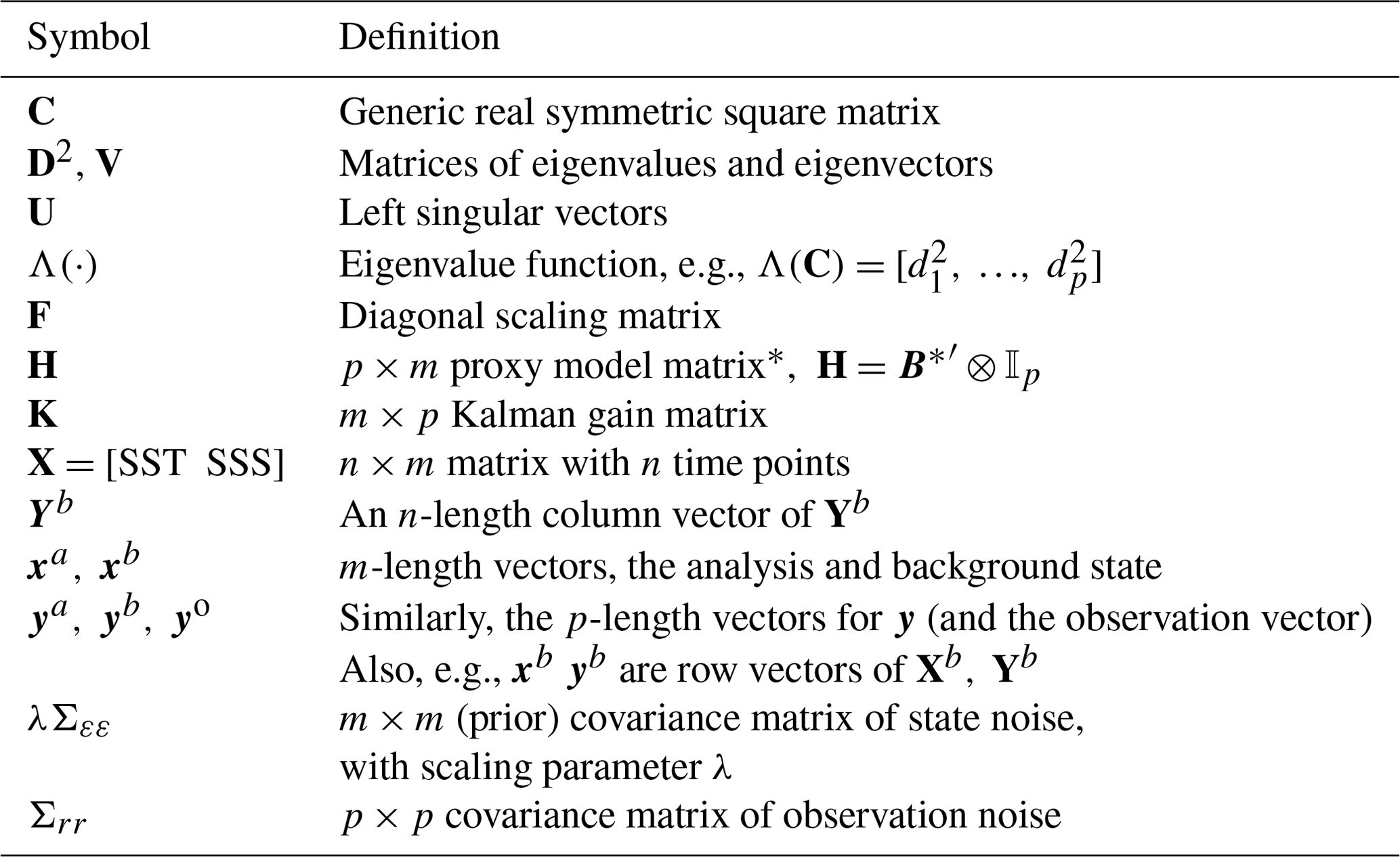
Table 1Notation used.
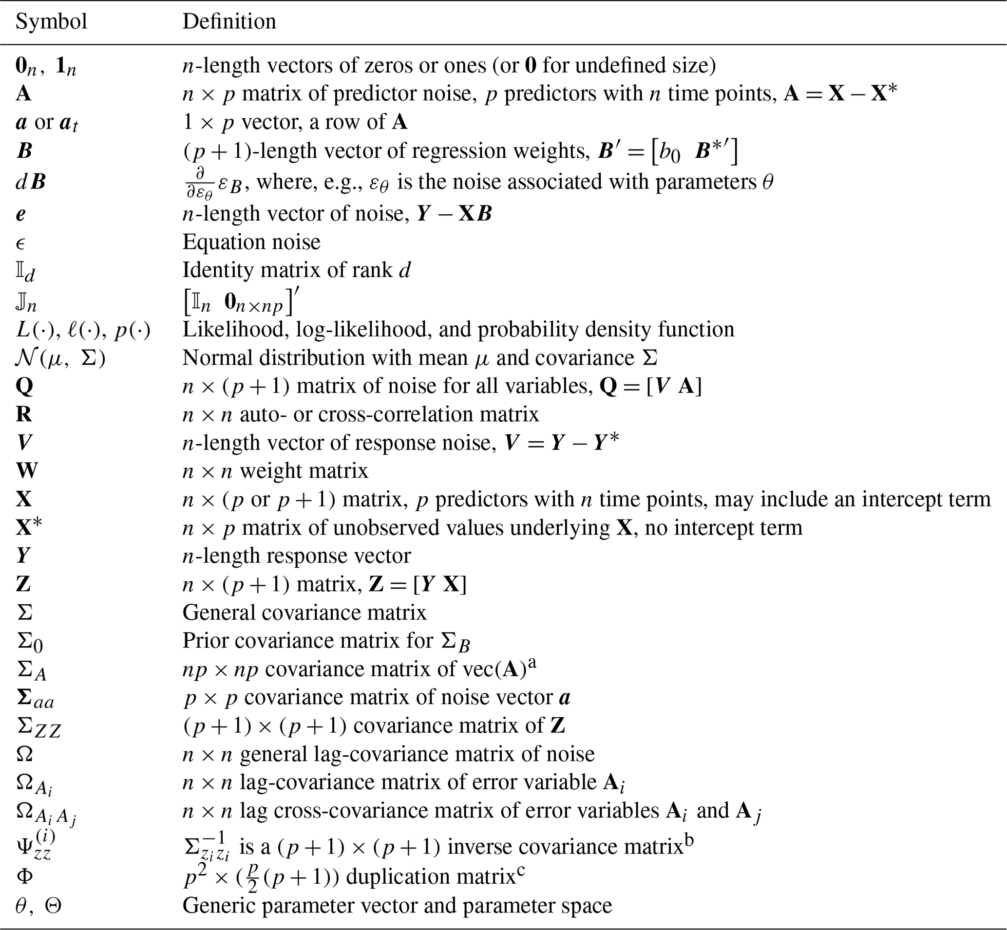
a The operator vec(A) means to column stack the matrix A (Henderson and Searle, 1979). b Superscript (i) refers to an index, rather than subscripting (e.g., ). c For the duplication matrix, see Magnus and Neudecker (1986).
Table 2Solutions for the EIV model. ΣA and ΣB are given in my notation.
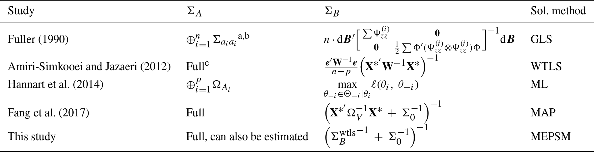
a The matrix direct sum operator ⊕ is notation to build a block diagonal matrix, e.g., . b Note though that technically , not ΣA, so ⊕ is used abstractly in this case. c Full: ΣA is not constrained to a particular type.
2.1 The EIV model
The general EIV model can be expressed as
Note that, for X* and B*, the superscript star also has a second use: it denotes that these entities do not include an intercept term, e.g., . From Eq. (3), the relevant covariance matrices are
and
See Appendix B for further information on covariance notation. These matrices describe a statistical stationary model. For example, the covariance matrix ΣA fully specifies the lag autocovariance and lag cross-covariances of the noise variables in A, but (ΣA)t=ΣA. Note this does not mean within ΣA that or (those are specific cases of ΣA). Also note that in this paper ΩV=ΣV. More will be said about ΣQ in Sect. 3.1.
Table 2 summarizes the main differences between previous solutions of the EIV model. First, these methods all assume that the equation noise ϵt (Eq. 3d) is either zero or not separate from vt. Earlier work by Fuller (1987) shows a way of including the equation noise separate from the response noise, but the predictor noise is limited to the p×p matrices . The solutions in Table 2 relate to generalized least squares (GLS), weighted total least squares (WTLS), maximum likelihood (ML), and maximum a posteriori (MAP) methods. A general estimator is of the following form:
where μZ is the GLS mean, , and . The covariance matrix is a weighted matrix, e.g., , but different ways of solving for B allow for different weightings. The assumption is then made that (e.g., Amiri-Simkooei and Jazaeri, 2012; Fang et al., 2017), despite the fact that different possible weightings exist. The ML method can be used to obtain a theoretically better estimation of ΣB, but it is computationally expensive if ΣA is not constrained. For example, in Hannart et al. (2014) ΣA is a block diagonal matrix: , where ⊕ is the direct sum operator for matrices (see Table 2 footnotes). The aim of the present study is to provide a solution for the EIV model that includes a fast theory-derived approximation of ΣB, a prior for ΣB, and a full ΣA, including a way to estimate ΣA with limited initial information.
2.2 MEPSM
As in previous studies, I also ignore the equation error, so the model in Eq. (3) can be re-expressed:
where , and (see Table 1 footnotes for the operator vec). The response variable is the first column of Z, denoted as Z1 or more generally as Y. Note also the two possible definitions of response noise for the model: and (where X includes an intercept term, to match with B). The difference is that
From , the covariance matrix of model prediction can be expressed as
Bayes' rule states that the posterior density function p(θ|𝒟) is proportional to the product of the likelihood function L(θ) and the prior density function p(θ):
Note that it does not matter if the likelihood function is a scaled distribution, e.g., a normal density function multiplied by a scalar (so it integrates to a number other than unity).
Assuming that the right-side distributions are Gaussian (or scaled Gaussian), then
where ml refers to the maximum likelihood solution. The posterior 𝒩(B, ΣB) integrates to unity, as expected. First I show an example by using the GLS likelihood. Let the GLS likelihood be
Now apply the Gaussian multiplication identity:
where . Thus the mean and variance of p(θ|𝒟) are
The above solution is a simple example using the GLS likelihood. To obtain the solution for the EIV problem, the GLS likelihood is replaced with the WTLS likelihood , where Bwtls and are derived in Appendix C and D. Using the WTLS likelihood, simplifying the product (from Eq. 13) is no longer feasible, so instead we write the mean and variance of p(θ|𝒟) simply as
2.3 Implementation
An application to calibrate a real PSM is provided in Sect. 3. Here general aspects of the solution and implementation are discussed.
The predictor noise and response noise, A and V, can be estimated as
Matrix A is needed for the calculation of both Bwtls and , while V is needed to re-estimate ΩV if relevant (see next paragraph).
The n×n covariance matrices (or ) and ΩV ideally need information about the cross-correlation within A and autocorrelation of A and V. If the ACF (autocorrelation function) and CCF (cross-correlation function) are not available, these can potentially be estimated using an iterative procedure. The procedure begins with vectors and , which are the heteroscedastic error variances (the diagonals of ΣA and ΩV).
3.1 A proxy system model, uncertainties, and the prior
A bivariate (i.e., two-predictor) PSM for coral δ18O is
where SST is sea surface temperature and SSS is sea surface salinity. Note that in the coral literature, the coefficients b1 and b2 are commonly referred to as a1 and a2, but here I use the former symbols for generality. This bivariate PSM has been used in data assimilation (Sanchez et al., 2021) and Monte Carlo experiments (Thompson et al., 2022). The bivariate PSM can be extended by rewriting it in the form of Eq. (7). The MEPSM requires estimates of the time-varying uncertainty of all variables and a prior distribution for B (see below). Here the time-varying uncertainties for the predictors are obtained from recent SST and SSS products that provide the complete uncertainty field , i.e., the uncertainty variance for each grid cell, at each time point.
For ERSSTv5, for each grid cell and time point, the SST total uncertainty is the sum of the parametric uncertainty and reconstruction uncertainty. These uncertainties are derived from a large reconstruction ensemble (Huang et al., 2020). The parametric uncertainty is based on the difference between the ensemble average and each ensemble member, given various internal parameters which affect SST uncertainty (including the uncertainty of the ship, buoy, or float measurement). The reconstruction uncertainty is based on the difference between each ensemble member and a pseudo-observation dataset on which the reconstruction method is trained, e.g., OISST (optimally interpolated SST). Note that the calculation of reconstruction uncertainty includes grid cells that have observational or no observational data, while the calculation of parametric uncertainty includes only grid cells that have observational data.
For HadEN4, the SSS total uncertainty is a combination of background uncertainty and observational uncertainty (Good et al., 2013). The observational uncertainty is obtained from previous studies, while the background uncertainty is the uncertainty associated with a persistent-based forecast.
For δ18Ocoral, the main known uncertainty is the analytical uncertainty, which is ∼0.05 ‰ for δ18Ocoral (Osborne et al., 2013). Time variation could be included by expressing the analytical uncertainty as a relative standard deviation of the mean δ18O (the effect of this will be tested elsewhere). Other uncertainties, which are unknown at many sites, include the intra- and inter-colony noise (Sayani et al., 2019). Note also that detrending adds time-varying uncertainty, because the trend uncertainty is larger at the ends of the time series (this is applicable to all detrended variables).
For MEPSM, the matrix ΣA can be initially constructed using Diag(σA⊙σA), where , “site” refers to the grid cell of a particular site, and the notation means over all time points. In the SST and SSS products, no information is given on the noise serial correlation, and no information exists on the noise cross-correlation between SST and SSS products. Seasonal peaks in the autocorrelation function (ACF) of SST noise could arise from, for example, seasonal changes in shipping tracks, which would affect the parametric uncertainty. Cross-correlation between SST and SSS noise might arise from sampling these variables at the same points within a particular grid cell (i.e., from the same ship) or due to seasonal variation in shipping tracks. Future work should investigate the ACF and CCF (cross-correlation function) for the SST and SSS ensembles (this is beyond the scope of the current paper). Finally, since the uncertainties in the predictors and response are fundamentally different, then ΣQ is assumed to be a block diagonal matrix, with ΩV and ΣA on the block diagonal and zero-filled blocks on the block anti-diagonal (Eq. 4).
For Bayesian methods, informative prior distributions are thought to be more useful than noninformative priors (Lemoine, 2019). For example, when using a fully noninformative prior distribution, the posterior distribution will be close to the maximum likelihood distribution, which would make using the fully noninformative prior somewhat obsolete.
The prior distribution for B is obtained from previous values that were used in Monte Carlo PSM experiments (Thompson et al., 2022; Watanbe and Pfeiffer, 2022). Those previous studies did not seek to calculate Bayesian posterior distributions, but the values in those studies represent current beliefs about the coefficients and their uncertainty and can be used as a prior. The prior distribution obtained from those studies is
where s=0.97 is a scaling factor between δ18Oseawater (in VSMOW) and δ18Ocoral (in VPDB). The values of and are from Thompson et al. (2022) and Watanbe and Pfeiffer (2022) respectively. The value of ‰ psu−1 originates from LeGrande and Schmidt (2006) and is an average ‰ per salinity value for the tropical Pacific Ocean. Regional variations in this value will probably be revealed by new datasets (DeLong et al., 2022), but for the purpose of this example of MEPSM, the value of 0.27 ‰ psu−1 is used. Thompson et al. (2022) considered two values for (i.e., ), so for this example an ”average” value is used (0.152). The value of the intercept b0 and its uncertainty are unknown in the sense that they are site-dependent values. A prior for these unknown values can be estimated by using the other prior coefficients and SST and SSS data for a particular site. For a particular site, the prior value of b0 can be calculated as
where and μy are the mean values of the predictors and response. From ordinary least squares theory, the diagonal elements of the covariance of B are typically given as
where is the error variance, and RSSj is the residual sum of squares after regressing Xj on X−j, where X−j is the matrix X omitting column j. So for ,
where X−0 is the observed part of X not including an intercept term (different than X*, which is the unobserved part of X). Preliminary analysis showed that the prior value for had a large influence on the posterior distribution of B, so only was scaled to be uninformative, i.e., .
3.2 Coral example
Rock Islands (7.27° N, 134.38° E) is a site on the western barrier reef of Palau, western Pacific Ocean. A number of coral cores were sampled from Rock Islands (RI) and the surrounding area, but the focus here is on one core labeled RI6, which is a monthly resolved record spanning 1899–2008. The core was sampled from a narrow-entrance lagoon, in shallow water (∼2 m depth). Osborne et al. (2013) compared the coral δ18O record with temperature data from the NCEP/NCAR Reanalysis (Kalnay et al., 1996) and salinity data from LEGOS (Delcroix et al., 2011). Using the raw (not detrended or deseasonalized) RI record from 1970–2008 and ordinary least squares, Osborne et al. (2013) regressed the coral δ18O against surface temperature and salinity, producing the following equation:
see Table A4 in Osborne et al. (2013). Osborne et al. (2013) attributed the small SST coefficient to the small seasonal SST range at Palau (∼1.5 °C), presumably because the small SST range makes the data scatter with δ18O more spherical than ellipsoid. They did not directly compare their raw SSS coefficient with any other data. Hence the RI δ18O record was chosen for this example, in order to further investigate the SST and SSS effects on coral δ18O at this site. In the following analysis the main differences with the analysis of Osborne et al. (2013) are that here the SST and SSS data are extracted from ERSSTv5 and HadEN4, because these products provide the uncertainty fields (Sect. 3.1). Secondly, the time period examined is from 1950–2008. Thirdly, for this study, all variables were detrended (using linear detrending and without removing the intercept), in order to ensure stationarity in the mean. For all variables, the trends at this site were weak. For example, for δ18Ocoral the trend from 1950–2008 was ‰ per year. A Jupyter Notebook with these preprocessing steps is available in the Supplement. Using this updated (and detrended) data, the OLS regression was recalculated as
Next MEPSM was applied to the same data, following the steps in Sect. 2.3. Except, for the application presented here, only ΣA was updated in step 4. ΩV was set as throughout, because here σV is thought to be mostly analytical noise, which should be approximately white (the uncertainty due to detrending is time-varying as well as white). For ΣA, for the auto- and cross-correlation functions of the predictor noise, up to 100 lags (months) were retained to construct the submatrices and (see Appendix E). Experiments with 50 and 150 lags showed little difference in the final posterior. In any application of MEPSM, the user should consider the source of the predictor and response noise in constructing ΣA and ΩV (as in Sect. 3.1).
Figure 1 shows the prior and the first and final posterior distributions for the SST and SSS coefficients. The first posterior distribution (dashed line) is obtained after step 2 (Sect. 2.3), while the final posterior is obtained after updating ΣA for auto- and cross-correlation. The (final) mean SST and SSS coefficients are given in Fig. 2: ‰ °C−1 and b2=0.49 ‰ psu−1. Figure 2 shows the marginal plots of the 3-dimensional scatter plot (SST, SSS, δ18O), together with the prior and posterior regression lines. For Rock Island, the SST and SSS coefficients are both steeper for the final posterior, compared to the OLS equation (Eq. 25).
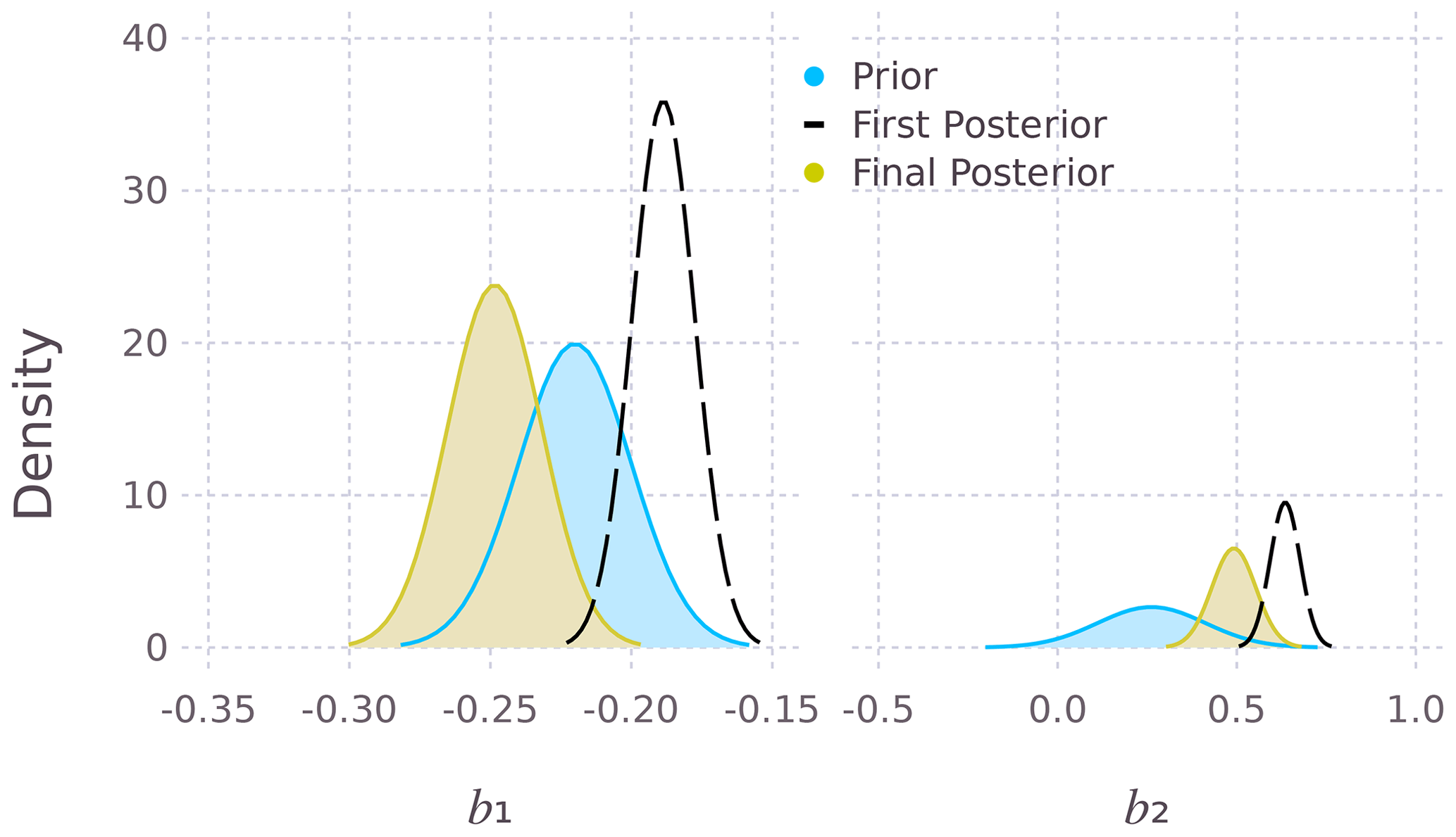
Figure 1The prior and posterior distributions for the SST (b1) and SSS (b2) coefficients. The final posterior is wider than the first posterior, because the final posterior accounts for auto- and cross-correlation in ΣA. In Figs. 1–3 the first posterior is the dashed line.
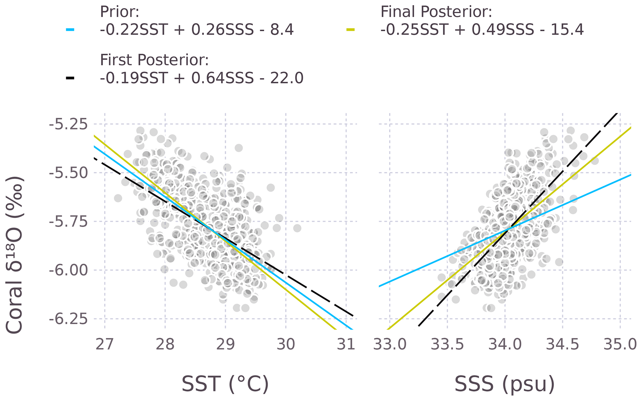
Figure 2The regression lines of the prior and posterior distributions. In 3 dimensions, these regression lines are the sides of a plane. Each shaded point corresponds to a monthly value from 1950–2008.
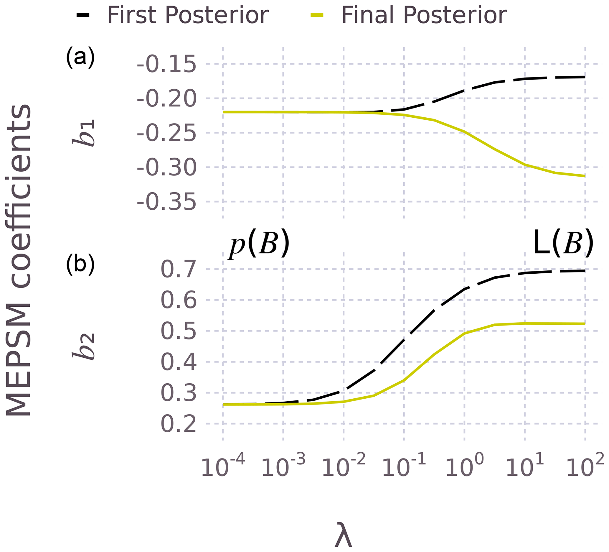
Figure 3The effect of the regularization parameter λ on the SST (b1, top) and SSS (b2, bottom) coefficients. The left and right side of the plots correspond to the prior distribution p(B) and likelihood distribution L(B) respectively.
Another advantage of Bayesian analysis is that attaching a ridge parameter λ to the prior variances means that the method can be used to regularize the solution, in a way that is different than traditional methods of regularization, such as principal component analysis, where components are retained by hard thresholding. Here, the ridge parameter λ is attached to the prior and allowed to vary over the range 10−4 to 102:
Figure 3 shows the effect of λ for both the first and final posterior. As λ increases, B moves from the prior distribution to the likelihood distribution. The difference between the solid and dashed lines (for each coefficient) is because of the effect of adjusting ΣA for auto- and cross-correlation, which becomes less relevant for small λ (). More will be said about serial dependence in A below. This type of prior regularization will likely be useful for sites where the (p+1)-dimensional scatter of data (predictors plus response) is more spherical than ellipsoid. For example, a more spherical scatter of data could occur at sites where the SST range is small. In practice, the value of λ could be estimated using cross-validation methods.
Table 3Regression parameters and their standard deviation, from four different solutions.
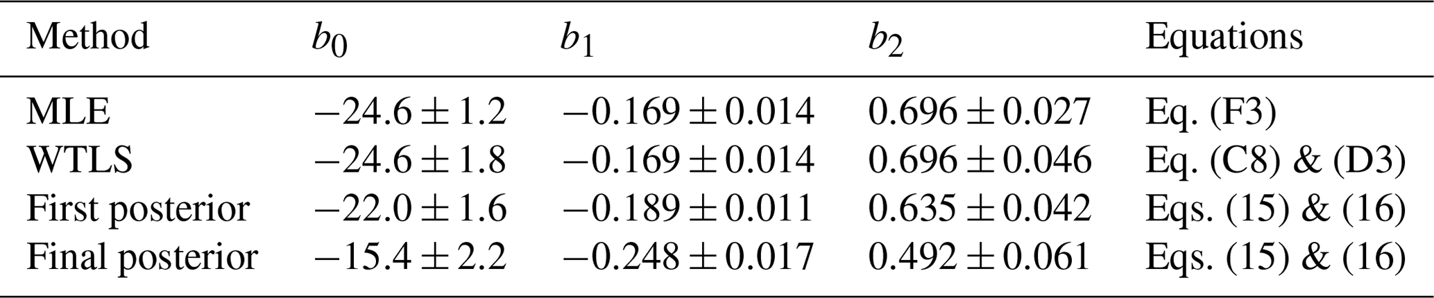
Table 3 compares the regression coefficients (and variance) from four different solutions: a ML solution (Appendix F), the WTLS method (Appendix C and D), and the MEPSM solution for the first and final posterior. The maximum likelihood estimate (MLE) and WTLS solution are basic implementations, i.e., no prior and no adjustment for autocorrelation or cross-correlation. The MLE and WTLS solutions are similar, with the variance being generally more conservative for WTLS, owing either to assumptions in the two methods or differences in method implementation, e.g., optimization for MLE versus analytical solution (with Gaussian assumptions) for WTLS. For the first posterior of MEPSM, both the mean and the variance move away from the WTLS solution and towards a tight prior: in Fig. 3 the MEPSM first posterior (on the dashed line) is the same as the λ=100 solution, and the basic WTLS solution is the same as λ≥102. For the final posterior (Table 3), the SST and SSS coefficients change steepness: b1 becomes steeper, while b2 becomes a little less steep compared to the WTLS solution and the first posterior (also seen in Fig. 3 as the difference between the solid and dashed lines). For both coefficients (Table 3), the variance increases for the final posterior (relative to the first posterior), because the final posterior adjusts for the auto- and cross-correlation in ΣA.
Figure 4 shows the autocorrelation of the noise in each variable (A1 is the SST noise, and A2 is the SSS noise), for the first and final posterior distribution. For the first posterior solution, the noise covariance in ΣA and ΩV is assumed to be heteroscedastic but white. This assumption is clearly not true, because all variables appear to have seasonally varying noise as shown by their autocorrelation functions (Fig. 4, left column). However, when this seasonally varying noise is included in ΣA (but not in ΩV), the response noise V essentially becomes white, as all the seasonal dependence moves into the predictor noise (Fig. 4, right column). Whether or not the response noise V should have seasonal variation (see Sect. 3.1) requires expert knowledge. This example is simply to illustrate the effect of including serially correlated noise in a multipredictor model. The implications of seasonally varying noise for coral PSMs will be addressed in another paper, with the application of MEPSM to a large coral database (Walter et al., 2023).
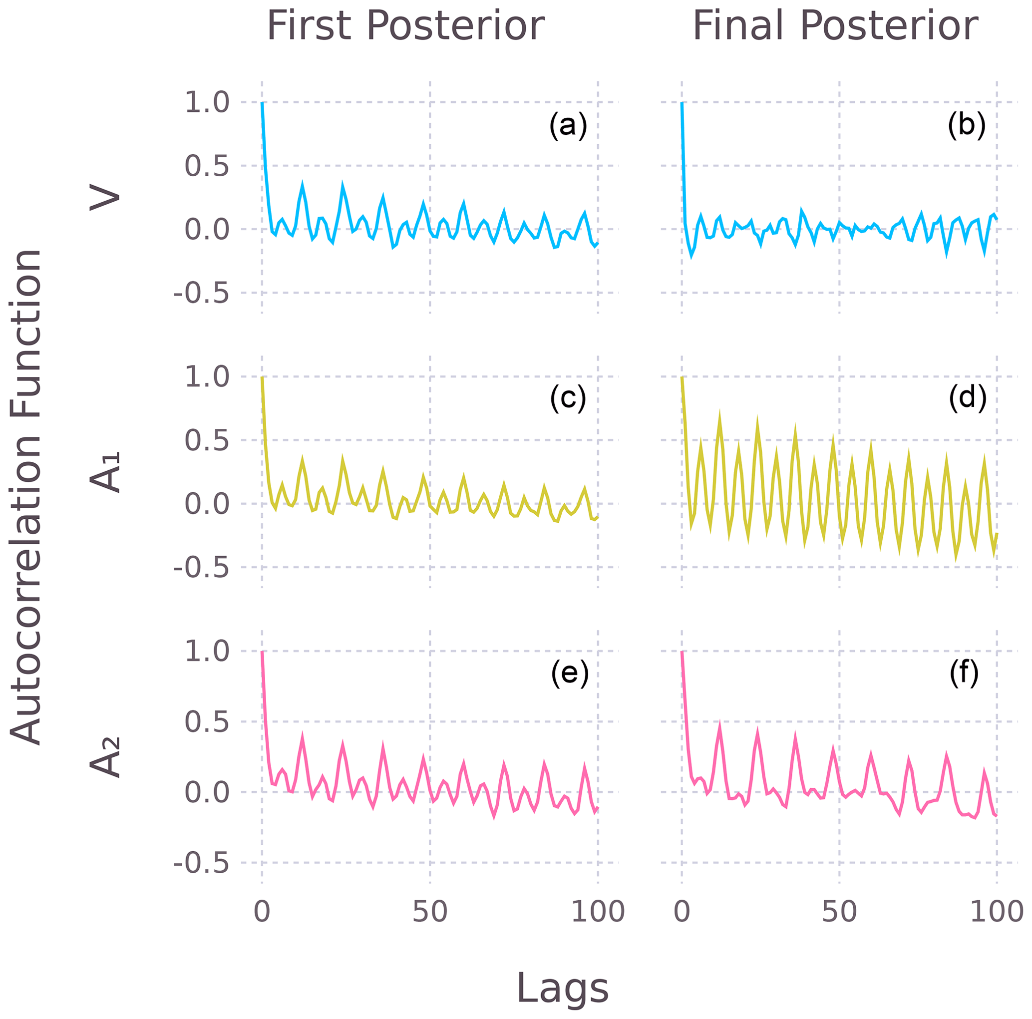
Table 4Notation for Sect. 3.3 (unless otherwise stated in text).
∗ In the experiments, p=5 and m=10 because there are two state variables and five grid points.
3.3 Data assimilation experiments
Two data assimilation (DA) experiments were performed using the Palau coral example. The purpose of these experiments is to investigate the effect of different H on data assimilation (Appendix G introduces DA and describes potential biases caused by misspecified H). For the experiments, the model prior covariance Σεε was obtained from iCESM1 (Brady et al., 2019), using a preindustrial run, and data from the last 400 years (1450–1850 CE, which is “closer” to the coral example period 1950–2007). Model SST and SSS data were extracted from a line of five grid cells, centered on the RI6 location. Although there is only one observational coral record, for these experiments, the same observational record is repeated for the five grid cells (Yo in DA). All data were deseasonalized but kept at monthly resolution. A line of grid cells was used, so the covariance Σεε includes some spatial correlation. The reasons for using covariance matrices in these experiments will become apparent. The covariances Σεε and Σrr were the same for both experiments and were constructed as follows:
-
, where is the singular value decomposition of X, k=1:3 (means the three leading eigencomponents), and denotes components filtered with a bandpass filter (2–20 years). Here interannual variability (as in Uk) is considered to be the state of interest. Filtering U better separates signal and noise.
-
, where and . This means that Σrr is a covariance matrix with the same correlation structure as HΣεεH′ but with variance scaling provided by , where V is from Eq. (18) (for DA, Var(V) is just the total variance of V). Also here , where Bpost2 denotes the values of B for the final posterior in Table 3. In the experiments below, keeping Σrr constant simplifies the comparisons.
To understand the experiment results, it is useful to cast data assimilation into observation space:
where , and xb, yo, and yb are treated like column vectors (to simplify the syntax). As expected, the analysis ya is a weighting between the prior and some likelihood 𝒩(yo, Σrr).
In both experiments that follow, the value of H in Eq. (27) changes (but not the value of Σrr, as defined above). Three different are tested, which are constructed from three values of B*: , , and (see Eq. 25 and Table 3). The difference between the two experiments is the value of yb=Hxb.
The data assimilation was implemented using a reduced-rank Kalman filter (Elbern et al., 2014) (rank reduction of Σεε is only used in Experiment 2). A notebook and code module for the experiments is available (Fischer, 2024). Note in the following subsections that V only refers to eigenvectors (see Table 4) and not the noise from MEPSM.
3.3.1 Experiment 1
In Experiment 1, xb (and thus yb) is set to zero. This mimics an offline DA situation where the model prior might be centered (i.e., zero mean) and constant. In addition, a scaling parameter λ is added to the prior, i.e., . If the prior covariance is large, then the prior is noninformative, and ya≈yo. Here a tighter prior is of interest, so λ is set to λ=0.1. Henceforth Σεε refers to a scaled prior covariance matrix, but the λ term is dropped.
.
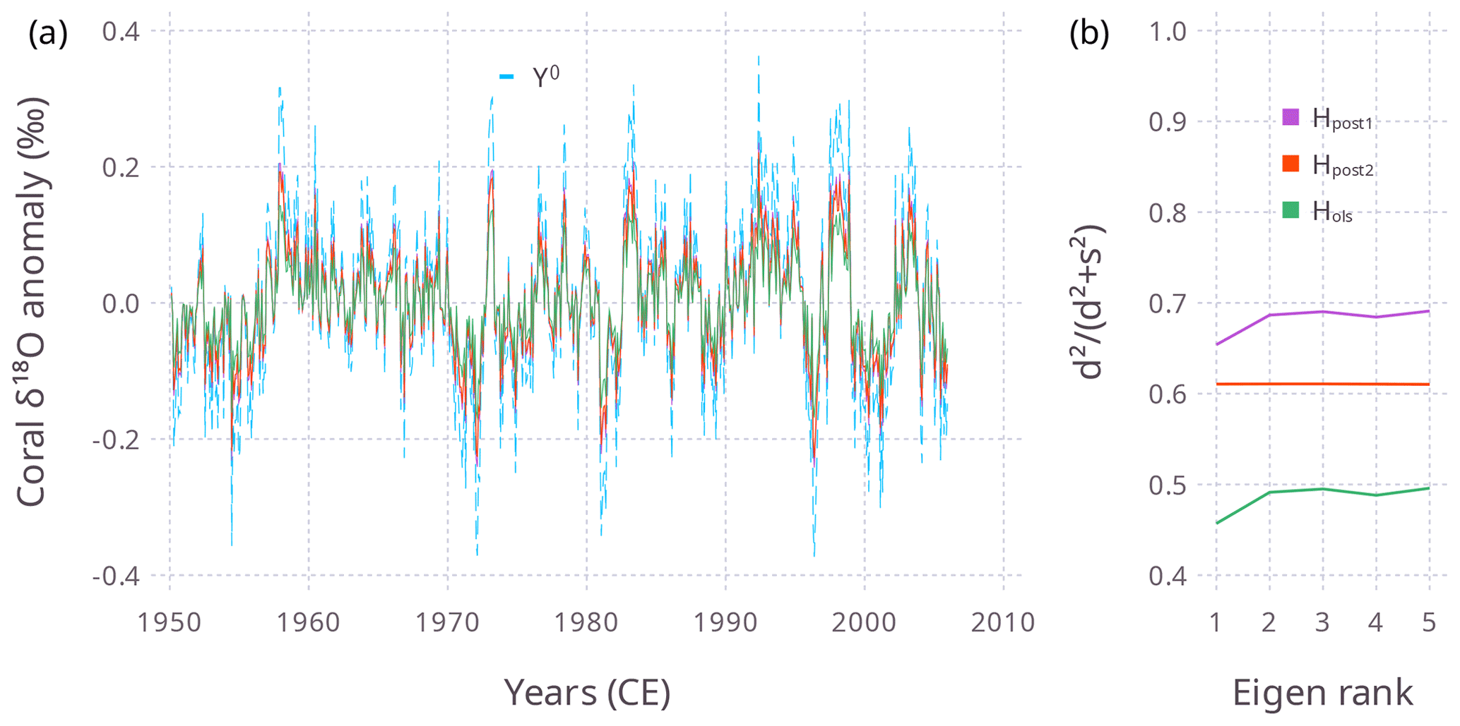
Figure 5For Experiment 1 (), (a) the time series Ya (solid lines, color key as in b) and (b) the eigenvalue shrinkage of the projection matrix (see text), for three different values of H. These experiments used five model grid points, but here Ya is plotted for the central grid point. In (a) the dashed line is Yo.
The DA posterior time series Ya is shown for the three different values of H in Fig. 5a, and the eigenvalue shrinkage (explained below) is shown in Fig. 5b. For λ=0.1, the Ya resulting from Hols shows the most shrinkage towards the zero-mean prior (Fig. 5a).
To understand the results from theory, two pieces of information are needed (see Table 4 for notation):
-
Λ(ΣC)=Λ(Σ0.5CΣ0.5), where Σ and C are real symmetric square matrices.
-
HΣεεH′ and Σrr have similar eigenvectors (because here Diag(F) is near constant) but different eigenvalues.
Setting yb to zero removes the Σrryb term in Eq. (27), leaving . The eigenvalues of the p×p projection matrix are of interest here. It follows (from the points above) that the projection matrix has the same eigenvalues as
where D2 and S2 are the eigenvalue matrices of HΣεεH′ and Σrr respectively. So in this example, the shrinkage factors of the projection matrix can be expressed as . Figure 5b shows that using Hols shrinks the eigenvalues more than for H from MEPSM. In this introductory experiment, the results have been examined in observation space; the next experiment will consider both xa and ya.
3.3.2 Experiment 2
In Experiment 2, model SST and SSS data were obtained for 1950–2005 from the iCESM historical run (which ended in 2005), for xb. The model data were deseasonalized and filtered using a low-pass (>2-year) filter (so here xb is a smooth prior, not a zero vector). This setup mimics data assimilation with a transient prior, e.g., offline data assimilation with time windows (windows are a type of prior smoothing). Note, for this experiment, that the model trajectory does not need to strongly match the observed historic trajectory. Further, Σεε is not a full rank matrix (the first three eigenvalues span 98% of the total variance), so for Experiment 2 only the first three leading components of Σεε are used (which helps to regularize Xa). Figure 6 shows, for λ=0.1, the three time series Yo, Yb, and Ya for each different H (named , where the latter two refer to the first and final posterior for MEPSM). Figure 6 shows the advantage of H from MEPSM is that, for example, yb=Hpost1xb has a greater range and thus allows ya to better capture the peaks and troughs in yo than can yb=Holsxb. To further compare the results for the different H, (Xa, Ya) was calculated for and compared with using the mean absolute error metric:
This was done similarly for . Note that , the estimated state from MEPSM, has no direct part in the DA.
Figure 7 shows that for this site, for Hpost2 (and Hpost1) the analysis and Ya typically have a smaller mae compared to Hols. Also, mae decreases as λ increases. For , the decrease flattens when ya≈yo (for λ>1, Fig. 7b), but note that Yo is not Y*. So in this example, it seems that a solution (Xa) better than the likelihood (yo=Hxa) cannot be achieved, which means that H from MEPSM wins (lower mae for ), because Hols biases (Fig. 7a). For Hols, there is less bias for , perhaps owing to the relative difference between OLS and MEPSM with respect to b2 (the SSS coefficient). Performing similar data assimilation experiments on global climate proxy datasets will better inform such issues and regional variation.
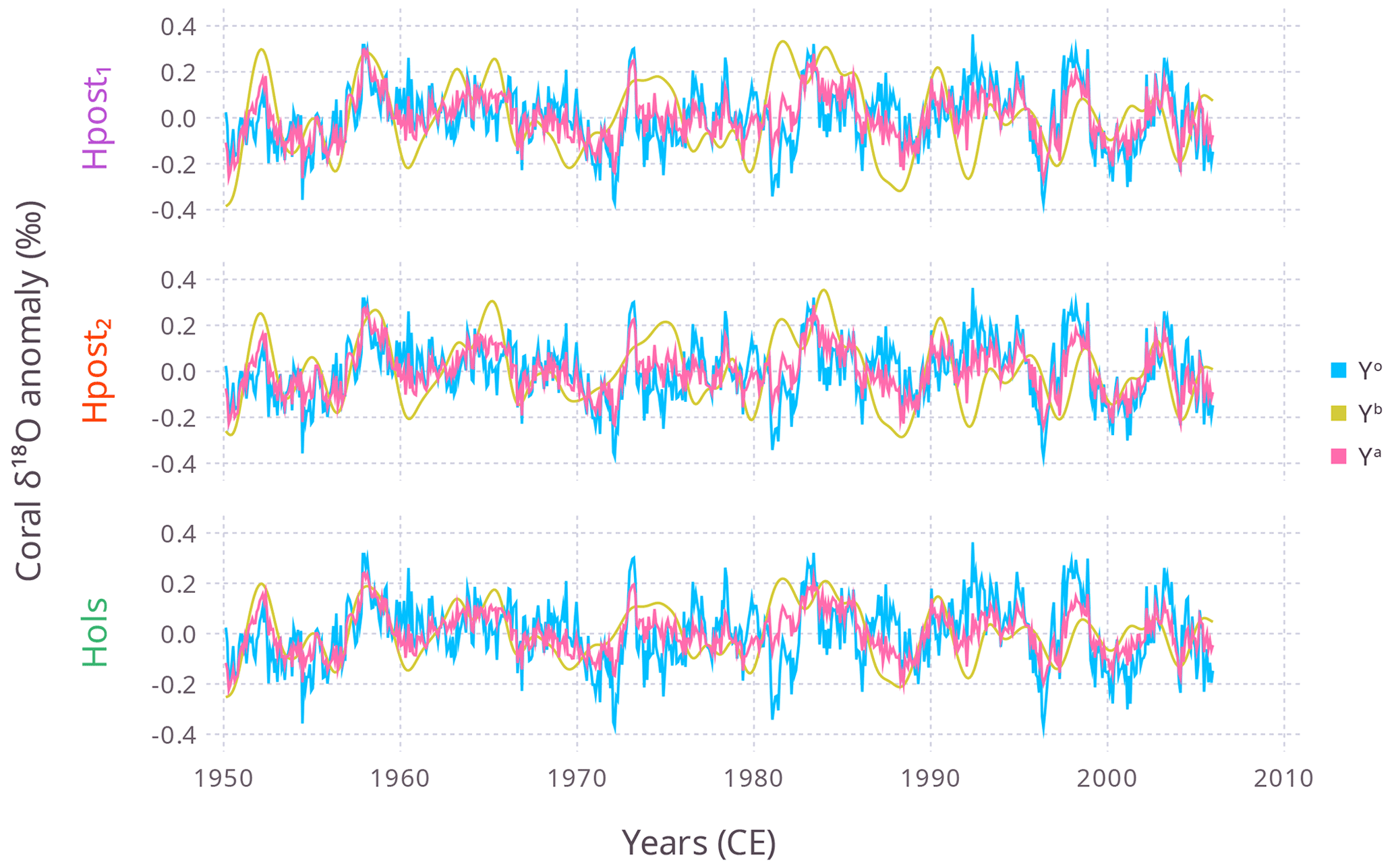
Figure 6For Experiment 2 (), the time series of Yo, Yb, and Ya (color key right) for three different H (on left axis). As in Fig. 5 Ya and Yb refer to the central grid point. In the panels, Yo is the same, but Yb and Ya depend on H. Note how ya is always between yb and yo.
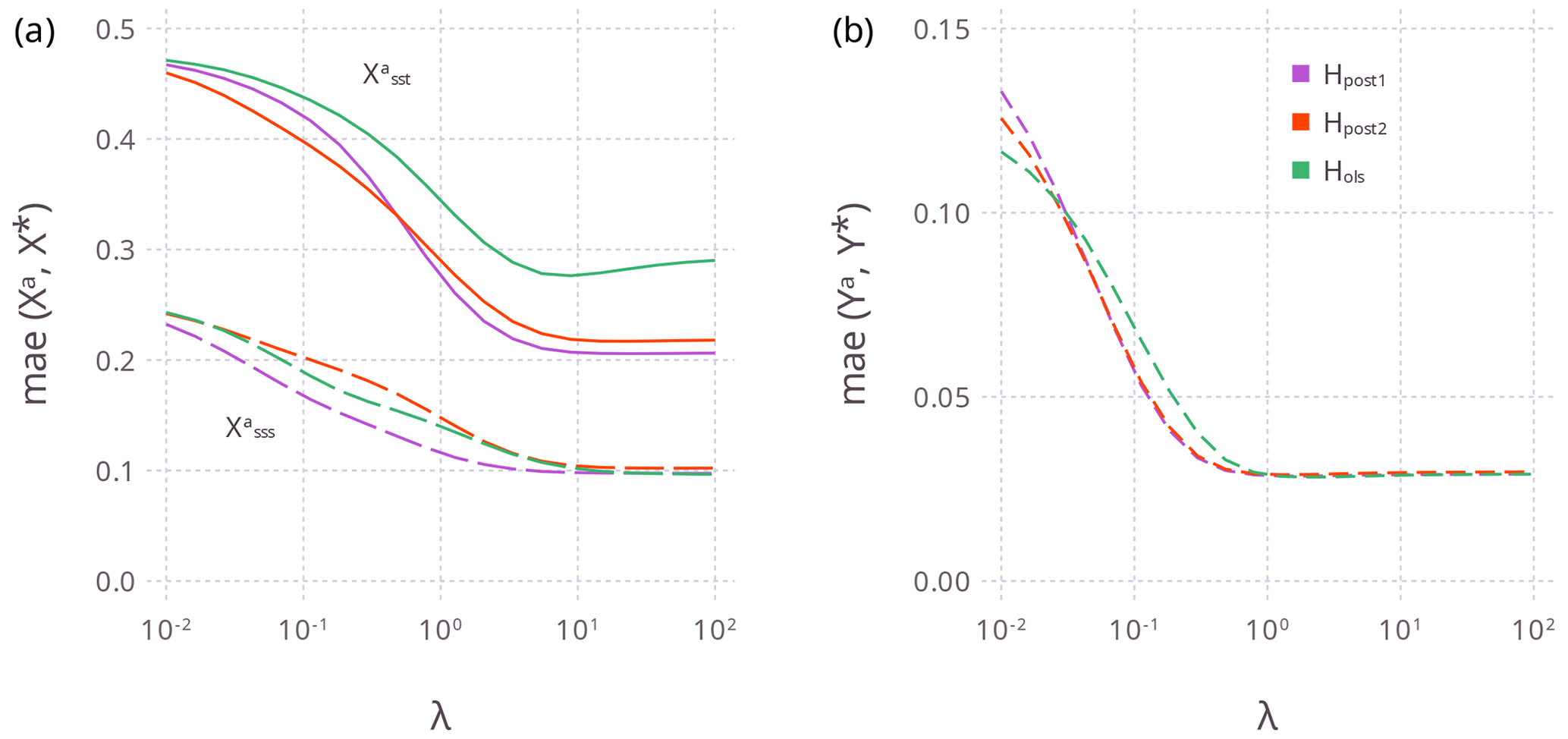
Figure 7For Experiment 2 (yb=Hxb), the mean absolute error for different λ for (a) Xa and (b) Ya (using the central grid point series) and for the three different H (color key as in b). Panel (a) shows the mae for (solid lines) and (long dashed lines), while panel (b) is the mae for Ya (see Eq. 29). Small values of λ mean ya≈yb, while large λ values mean ya≈yo.
MEPSM is a new type of proxy system model which incorporates both prior information and generalized noise in all variables, such as cross-correlated noise within the predictor variables. DA theory and two experiments suggest that, in data assimilation, the MEPSM should have an advantage over conventional OLS-calibrated PSMs (the latter are widely employed in current paleo-DA projects). In the work presented here for MEPSM, the response noise is assumed to be independent of the predictor noise (the zero matrices in ΣQ), but cross-correlation between the predictor and response noise is possible (if needed), by complete quadratic multiplication of ΣQ, rather than treating ΩV and ΣA separately, in Eq. (9). However, for many PSMs the predictor and response noise are fundamentally different and therefore should be independent. The next step is to apply MEPSM to calibrate multiple-input proxy system models for different climate proxies (e.g., isotopes in corals, tree rings, and speleothems) and to incorporate MEPSM into current data assimilation projects.
Let
A first-order Taylor expansion gives
such that the variance of f(x) is . The first-order Taylor expansion will be exact when f(x) is a linear function.
Covariance can be given in plain or scaled format, e.g.,
So, just as an example, a naive covariance matrix for B could be written as follows:
In this paper I use the plain format because it simplifies many expressions.
The target function for WTLS essentially consists of the quadratic component of the log-likelihood function:
where . For , Eq. (C1) reduces to
where . Next substitute V with Eq. (18):
The residual vector e can be written as
or
Then setting Eq. (C3) to zero, substituting for e, and rearranging gives
or
where A now may include a column of zeros (corresponding to noiseless predictors in X).
Equation (C7) expands to
where () is the weighted covariance between A and the predictors, and () is the weighted covariance between A and the response vector. This shows that WTLS can be expressed as an adjusted least squares problem. Hence, it can also be expressed as an augmented linear regression:
which is equivalent to Eq. (7).
For two predictors, ΣA is
ΣA can be constructed as
where Diag(⋅) is a diagonal matrix, and σA is a (n⋅p)-length vector containing the heteroscedastic “variance” of the predictor noise for each predictor (stacked vertically). The central block matrix, made up of submatrices R, will be labeled . The submatrices of are n×n correlation matrices, containing the autocorrelation or cross-correlation information for the predictor noise A:
where is the auto- or cross-correlation function.
If R is an autocorrelation matrix, then ρ0=1. Also, because the auto- or cross-correlation may become ∼0 at long lags, then ρ>k may be set to 0, for a chosen lag k. To ensure that is positive definite, the algorithm of Rebonato and Jaeckel (1999) is computationally fast.
ΩV can be similarly constructed:
Hannart et al. (2014) defined the log-likelihood of the EIV model as (here written using the notation in this paper, rather than the notation of Hannart et al., 2014)
which is a reduced form of Eq. (C1), because the off-diagonal matrices in ΣA are not included. Hannart et al. (2014) wrote an iterative (fixed-point) solution in terms of X* and B*.
where here , and . (I have included the intercept b0 explicitly.) Confidence intervals for each bi were calculated from the likelihood profiles (see Sect. 3 in Hannart et al., 2014).
The ML solution I provide here differs from Hannart et al. (2014), but I adopt a similar form (what follows is only for the ML estimate in the first row of Table 3). I express the log-likelihood in Eq. (F1) as a function of V and A:
where A and V are calculated using Eqs. (17)–(18). The difference with Hannart et al. (2014) is that the likelihood here is rewritten with respect to (through Eqs. 17–18), whereas the procedure of Hannart et al. (2014) is expressed with respect to , i.e., the main difference being X or X*. The point here is merely to provide a basic ML solution in Table 3, in order to compare with the other solutions. Equation (F3) should work with many standard ML packages, because there is no iterative dependence on X*.
The first row in Table 3 was calculated using Eq. (F3), and the Julia package ProfileLikelihoods.jl (VandenHeuvel, 2022).
This appendix explores the potential advantages of MEPSM for paleodata assimilation (PDA). This is a stand-alone appendix, and notation may differ from the main text. The following notation is used for the data assimilation components:
-
xb is the climate model data, at m grid points.
-
y is the proxy data, at p grid points.
-
θ is the unobserved state vector, with m grid points.
-
H is the operator which converts model space to proxy space.
Matrix H is p×m. (Note that if a proxy system model has multiple inputs, then H can be formed by concatenation, e.g., H=[Hsst Hsss] in which case m above becomes 2m.).
Data assimilation can be expressed in GLS format:
where and . In the typical offline PDA, Σεε is an m×m background covariance matrix. In MEPSM, the predictor noise matrix is ΣA. Out of interest, a time-constant noise matrix could be specified as . Note the difference between Σεε and Σaa: Σεε is estimated from climate model ensembles, whereas Σaa is from ensemble climate data reconstructions (e.g., an ensemble SST product). Also, PDA is about estimating θ, whereas MEPSM is about calibrating H (in MEPSM B contains the non-zero elements of H). Note that H is typically calibrated using observed modern climate data and proxies, over a coeval period (e.g., the 20th century). I will say more about H below.
Next concatenate the two equations above into one:
where , and let . The GLS solution for θ is
For the analysis error covariance Σa, it is
Equation (G4) can also be expanded as
where . The question here is what happens if H is calibrated using a biased method (e.g., OLS). Equation (G4) suggests that Σa will also be biased. Ensemble filtering methods are used for their computational advantage: replacing a large m×m Σεε with a smaller ensemble of model xb vectors. But the model xb vectors are filtered in a way that ensures the resulting ensemble of δθa (i.e., deviation from ) agrees with Eq. (G5). So ensemble filtering methods do not help if H is biased. Equation (G1) shows that the operator H is applied to the unobserved state θ, not to the “observed” xb, so using OLS for calibrating H seems flawed. OLS calibrates a PSM on observed (but not true) data, whereas MEPSM calibrates a PSM on the unobserved state x*.
Intuitive Julia code for MEPSM is available on GitHub (https://github.com/Mattriks/MeasurementErrorModels.jl, last access: 2 April 2023) and Zenodo (https://doi.org/10.5281/zenodo.7793741, Fischer, 2023a). A manual for MEPSM is available at https://mattriks.github.io/MeasurementErrorModels.jl/dev/ (Fischer, 2023b). The manual contains three examples which reproduce results from this paper.
The ERSSTv5 sea surface temperature data are available at https://psl.noaa.gov/data/gridded/data.noaa.ersst.v5.html (last access: 16 December 2019) (metadata: https://doi.org/10.7289/V5T72FNM, Huang et al., 2017). The ERSSTv5 uncertainty data were obtained from Boyin Huang, NOAA (22 October 2020).
The HadEN4 ocean salinity data (and uncertainty) are available at https://apdrc.soest.hawaii.edu/las/v6/dataset?catitem=16652 (Gouretski and Reseghetti, 2020). These data are from version EN.4.2.1 and are the G10 analyses, i.e., with the corrections of Gouretski and Reseghetti (2010).
The coral δ18O data from core RI6 were extracted from the CoralHydro2k database (Walter et al., 2023). A Jupyter Notebook (as a PDF) showing the preprocessing of these data is available in the Supplement. The dataset stored for the code examples in the GitHub repository contains all three detrended variables (detrended without removing the intercept).
Some input variables for PSMs, from the iCESM1 last millennium simulation (Brady et al., 2019), are available at the University of Washington (https://atmos.washington.edu/~rtardif/LMR/prior, Tardif, 2024). The variables ocean surface temperature (tos_sfc) and ocean surface salinity (sos_sfc) are used in Sect. 3.3.
A notebook and code module for Sect. 3.3 are available on Zenodo (https://doi.org/10.5281/zenodo.12660485, Fischer, 2024).
The supplement related to this article is available online at: https://doi.org/10.5194/gmd-17-6745-2024-supplement.
The author has declared that there are no competing interests.
Publisher's note: Copernicus Publications remains neutral with regard to jurisdictional claims made in the text, published maps, institutional affiliations, or any other geographical representation in this paper. While Copernicus Publications makes every effort to include appropriate place names, the final responsibility lies with the authors.
I thank the reviewers for useful suggestions that helped to improve the manuscript.
This paper was edited by Marko Scholze and reviewed by two anonymous referees.
Amiri-Simkooei, A. and Jazaeri, S.: Weighted total least squares formulated by standard least squares theory, Journal of Geodetic Science, 2, 113–124, https://doi.org/10.2478/v10156-011-0036-5, 2012. a, b
Brady, E., Stevenson, S., Bailey, D., Liu, Z., Noone, D., Nusbaumer, J., Otto-Bliesner, B. L., Tabor, C., Tomas, R., Wong, T., Zhang, J., and Zhu, J.: The Connected Isotopic Water Cycle in the Community Earth System Model Version 1, J. Adv. Model. Earth Sy., 11, 2547–2566, https://doi.org/10.1029/2019MS001663, 2019. a, b
Dee, S.: PRYSM: An open-source framework for PRoxY System Modeling, with applications to oxygen-isotope systems, Adv. Model. Earth Sy., 7, 1220–1247, https://doi.org/10.1002/2015MS000447, 2015. a
Delcroix, T., Alory, G., Cravatte, S., Corrège, T., and McPhaden, M. J.: A gridded sea surface salinity data set for the tropical Pacific with sample applications (1950–2008), Deep-Sea Res. Pt. I, 58, 38–48, https://doi.org/10.1016/j.dsr.2010.11.002, 2011. a
DeLong, K. L., Atwood, A., Moore, A., and Sanchez, S.: Clues from the sea paint a picture of Earth's water cycle, Eos, 103, https://doi.org/10.1029/2022EO220231, 2022. a
Elbern, H., Friese, E., Nieradzik, L., and Schwinger, J.: Data assimilation in atmospheric chemistry and air quality, in: Advanced Data Assimilation for Geosciences: Lecture Notes of the Les Houches School of Physics: Special Issue, June 2012, Oxford University Press, https://doi.org/10.1093/acprof:oso/9780198723844.003.0022, 2014. a
Evans, M. N., Tolwinski-Ward, S. E., Thompson, D. M., and Anchukaitis, K. J.: Applications of proxy system modeling in high resolution paleoclimatology, Quaternary Sci. Rev., 76, 16–28, https://doi.org/10.1016/j.quascirev.2013.05.024, 2013. a
Fang, X., Li, B., Alkhatib, H., Zeng, W., and Yao, Y.: Bayesian Inference for the Errors-In-Variables model, Stud. Geophys. Geod., 61, 35–52, https://doi.org/10.1007/s11200-015-6107-9, 2017. a, b
Fischer, M.: Mattriks/MeasurementErrorModels.jl: MEPSM v0.2.0, Zenodo [code], https://doi.org/10.5281/zenodo.7793741, 2023a. a
Fischer, M.: Measurement Error Proxy System Models: MEPSM v0.2, Model documentation, https://mattriks.github.io/MeasurementErrorModels.jl/dev/ (last access: 2 April 2023), 2023b. a
Fischer, M.: Data assimilation notebook and code module, Zenodo [code], https://doi.org/10.5281/zenodo.12660485, 2024. a, b
Florens, J.-P., Mouchart, M., and Richard, J.-F.: Bayesian inference in Errors-in-Variables Models, J. Multivariate Anal., 4, 419–452, https://doi.org/10.1007/s11200-015-6107-9, 1974. a
Fuller, W. A.: Chapter 3: Extensions of the single relation model, in: Measurement Error Models, John Wiley & Sons, https://doi.org/10.1002/9780470316665.ch3, 1987. a
Fuller, W. A.: Prediction of true values for the measurement error model, in: Statistical Analysis of Measurement Error Models and Applications, edited by: Brown, P. J. and Fuller, W. A., American Mathematical Society, 41–58, https://doi.org/10.1090/conm/112/1087098, 1990. a
Good, S. A., Martin, M. J., and Rayner, N. A.: EN4: Quality controlled ocean temperature and salinity profiles and monthly objective analyses with uncertainty estimates, J. Geophys. Res.-Oceans, 118, 6704–6716, https://doi.org/10.1002/2013JC009067, 2013. a
Gouretski, V. and Reseghetti, F.: On depth and temperature biases in bathythermograph data: Development of a new correction scheme based on analysis of a global ocean database, Deep-Sea Res. Pt. I, 57, 812–833, https://doi.org/10.1016/j.dsr.2010.03.011, 2010. a
Gouretski, V. and Reseghetti, F.: HadEN4 salinity and salinity error standard deviation data, Asia-Pacific Data-Research Center [data set], https://apdrc.soest.hawaii.edu/las/v6/dataset?catitem=16652, last access: 11 November 2020. a
Hannart, A., Ribes, A., and Naveau, P.: Optimal fingerprinting under multiple sources of uncertainty, Geophys. Res. Lett., 41, 1261–1268, https://doi.org/10.1002/2013GL058653, 2014. a, b, c, d, e, f, g, h, i, j, k, l
Henderson, H. V. and Searle, S. R.: Vec and vech operators for matrices, with some uses in jacobians and multivariate statistics, Can. J. Stat., 7, 65–81, https://doi.org/10.2307/3315017, 1979. a
Huang, B., Thorne, P. W., Banzon, V. F., Boyer, T., Chepurin, G., Lawrimore, J. H., Menne, M. J., Smith, T. M., Vose, R. S., and Zhang, H.-M.: NOAA Extended Reconstructed Sea Surface Temperature (ERSST), Version 5, NOAA National Centers for Environmental Information [data set], https://doi.org/10.7289/V5T72FNM, 2017. a
Huang, B., Menne1, M. J., Boyer, T., Freeman, E., Gleason, B. E., Lawrimore, J. H., Liu, C., Rennie III, J. J., C. J. S., Sun, F., Vose1, R., Williams, C. N., Yin, X., and Zhang, H.-M.: Uncertainty Estimates for Sea Surface Temperature and Land Surface Air Temperature in NOAAGlobalTemp Version 5, J. Climate, 33, 1351–1379, https://doi.org/10.1175/JCLI-D-19-0395.1, 2020. a
Kalnay, E., Kanamitsu, M., Kistler, R., Collins, W., Deaven, D., Gandin, L., Iredell, M., Saha, S., White, G., Woollen, J., Zhu, Y., Chelliah, M., Ebisuzaki, W., Higgins, W., Janowiak, J., Mo, K. C., Ropelewski, C., Wang, J., Leetmaa, A., Reynolds, R., Jenne, R., and Joseph, D.: The NCEP/NCAR 40-Year Reanalysis Project, B. Am. Meteorol. Soc., 77, 437–471, https://doi.org/10.1175/1520-0477(1996)077<0437:TNYRP>2.0.CO;2, 1996. a
King, J., Tierney, J., Osman, M., Judd, E. J., and Anchukaitis, K. J.: DASH: a MATLAB toolbox for paleoclimate data assimilation, Geosci. Model Dev., 16, 5653–5683, https://doi.org/10.5194/gmd-16-5653-2023, 2023. a, b, c
LeGrande, A. N. and Schmidt, G. A.: Global gridded data set of the oxygen isotopic composition in seawater, Geophys. Res. Lett., 33, L12604, https://doi.org/10.1029/2006GL026011, 2006. a
Lemoine, N. P.: Moving beyond noninformative priors: why and how to choose weakly informative priors in Bayesian analyses, Oikos, 128, 912–928, https://doi.org/10.1111/oik.05985, 2019. a
Loope, G., Thompson, D. M., Cole, J., and Overpeck, J.: Is there a low-frequency bias in multiproxy reconstructions of tropical pacific SST variability?, Quaternary Sci. Rev., 246, 106530, https://doi.org/10.1016/j.quascirev.2020.106530, 2020a. a
Loope, G., Thompson, D. M., and Overpeck, J.: The spectrum of Asian Monsoon variability: a proxy system model approach to the hydroclimate scaling mismatch, Quaternary Sci. Rev., 240, 106362, https://doi.org/10.1016/j.quascirev.2020.106362, 2020b. a
Ludwig, K. R. and Titterington, D. M.: Calculation of 230ThU isochrons, ages, and errors, Geochim. Cosmochim. Ac., 58, 5031–5042, https://doi.org/10.1016/0016-7037(94)90229-1, 1994. a
Magnus, J. R. and Neudecker, H.: Symmetry, 0-1 Matrices and Jacobians, Econometric Theory, 2, 157–190, https://doi.org/10.1017/S0266466600011476, 1986. a
Malevich, S. B., Vetter, L., and Tierney, J. E.: Global Core Top Calibration of δ18O in Planktic Foraminifera to Sea Surface Temperature, Paleoceanogr. Paleocl., 34, 1292–1315, https://doi.org/10.1029/2019PA003576, 2019. a
Osborne, M. C., Dunbar, R. B., and Mucciarone, D. A.: Regional calibration of coral-based climate reconstructions from Palau, West Pacific Warm Pool, Palaeogeogr. Palaeocl., 386, 308–320, https://doi.org/10.1016/j.palaeo.2013.06.001, 2013. a, b, c, d, e, f
Rebonato, R. and Jaeckel, P.: The most general methodology to create a valid correlation matrix for risk management and option pricing purposes, J. Risk, 2, 17–27, https://doi.org/10.21314/JOR.2000.023, 1999. a
Sanchez, S. C., Hakim, G. J., and Sanger, C. P.: Climate Model Teleconnection Patterns Govern the Niño-3.4 Response to Early Nineteenth-Century Volcanism in Coral-Based Data Assimilation Reconstructions, J. Climate, 34, 1863–1880, https://doi.org/10.1175/JCLI-D-20-0549.1, 2021. a, b
Sayani, H. R., Cobb, K. M., DeLong, K., Hitt, N. T., and Druffel, E. R. M.: Intercolony δ18O and Sr/Ca variability among Porites spp. corals at Palmyra Atoll: Toward more robust coral-based estimates of climate, Geochem. Geophys. Geosyst., 20, 5270–5284, https://doi.org/10.1029/2019GC008420, 2019. a
Schneider, T.: Analysis of Incomplete Climate Data: Estimation of Mean Values and Covariance Matrices and Imputation of Missing Values, J. Climate, 14, 853–871, https://doi.org/10.1175/1520-0442(2001)014<0853:AOICDE>2.0.CO;2, 2001. a
Steiger, N. J., Smerdon, J. E., Cook, E. R., and Cook, B. I.: A reconstruction of global hydroclimate and dynamical variables over the Common Era, Sci. Data, 5, 180086, https://doi.org/10.1038/sdata.2018.86, 2018. a, b
Tardif, R.: The post-processed “iCESM1” last millennium simulation, atmos.washington [data set], https://atmos.washington.edu/~rtardif/LMR/prior, last access: 14 June 2024. a
Tardif, R., Hakim, G. J., Perkins, W. A., Horlick, K. A., Erb, M. P., Emile-Geay, J., Anderson, D. M., Steig, E. J., and Noone, D.: Last Millennium Reanalysis with an expanded proxy database and seasonal proxy modeling, Clim. Past, 15, 1251–1273, https://doi.org/10.5194/cp-15-1251-2019, 2019. a, b
Thompson, D. M., Conroy, J. L., Konecky, B. L., Stevenson, S., DeLong, K. L., McKay, N., Reed, E., Jonkers, L., and Carré, M.: Identifying Hydro-Sensitive Coral δ18O Records for Improved High-Resolution Temperature and Salinity Reconstructions, Geophys. Res. Lett., 49, e2021GL096153, https://doi.org/10.1029/2021GL096153, 2022. a, b, c, d
Tierney, J. E. and Tingley, M. P.: A Bayesian, spatially-varying calibration model for the TEX86 proxy, Geochim. Cosmochim. Ac., 127, 83–106, https://doi.org/10.1016/j.gca.2013.11.026, 2014. a
Tierney, J. E. and Tingley, M. P.: BAYSPLINE: A New Calibration for the Alkenone Paleothermometer, Paleoceanogr. Paleocl., 33, 281–301, https://doi.org/10.1002/2017PA003201, 2018. a
Tierney, J. E., Malevich, S. B., Gray, W., Vetter, L., and Thirumalai, K.: Bayesian Calibration of the Mg/Ca Paleothermometer in Planktic Foraminifera, Paleoceanogr. Paleocl., 34, 2005–2030, https://doi.org/10.1029/2019PA003744, 2019. a
VandenHeuvel, D.: DanielVandH/ProfileLikelihood.jl: v0.2.1, Zenodo [code], https://doi.org/10.5281/zenodo.7493449, 2022. a
Walter, R. M., Sayani, H. R., Felis, T., Cobb, K. M., Abram, N. J., Arzey, A. K., Atwood, A. R., Brenner, L. D., Dassié, É. P., DeLong, K. L., Ellis, B., Emile-Geay, J., Fischer, M. J., Goodkin, N. F., Hargreaves, J. A., Kilbourne, K. H., Krawczyk, H., McKay, N. P., Moore, A. L., Murty, S. A., Ong, M. R., Ramos, R. D., Reed, E. V., Samanta, D., Sanchez, S. C., Zinke, J., and the PAGES CoralHydro2k Project Members: The CoralHydro2k database: a global, actively curated compilation of coral δ18O and proxy records of tropical ocean hydrology and temperature for the Common Era, Earth Syst. Sci. Data, 15, 2081–2116, https://doi.org/10.5194/essd-15-2081-2023, 2023. a, b
Watanbe, T. K. and Pfeiffer, M.: A Simple Monte Carlo Approach to Estimate the Uncertainties of SST and δ18Osw Inferred From Coral Proxies, Geochem. Geophys. Geosyst., 23, e2021GC009813, https://doi.org/10.1029/2021GC009813, 2022. a, b
York, D.: Least-squares fitting of a straight line, Can. J. Phys., 44, 1079–1086, https://doi.org/10.1139/p66-090, 1966. a
York, D.: Least-squares fitting of a straight line with correlated errors, Earth Planet. Sci. Lett., 5, 320–324, https://doi.org/10.1016/S0012-821X(68)80059-7, 1968. a
- Abstract
- Introduction
- Methods
- Application
- Conclusions
- Appendix A: Basis of Eq. (2)
- Appendix B: Notation for covariance
- Appendix C: The WTLS likelihood and its mean Bwtls
- Appendix D: Covariance of Bwtls
- Appendix E: Construction of ΣA and ΩV
- Appendix F: Maximum likelihood solution of Hannart et al. (2014)
- Appendix G: MEPSM and paleodata assimilation
- Code and data availability
- Competing interests
- Disclaimer
- Acknowledgements
- Review statement
- References
- Supplement